Nature and origin of the operators entering the master equation of an open quantum system

Abstract

By exploiting the peculiarities of a recently introduced formalism for describing open quantum systems (the Parametric Representation with Environmental Coherent States) we derive an equation of motion for the reduced density operator of an open quantum system that has the same structure of the celebrated
Gorini–Kossakowski–Sudarshan–Lindblad equation, but holds regardless of markovianity being assumed. The operators in our result have explicit expressions in terms of the Hamiltonian describing the interactions with the environment, and can be computed once a specific model is considered. We find that, instead of a single set of Lindblad operators, in the general (non-markovian) case there one set of Lindblad-like operators for each and every point of a symplectic manifold associated to the environment. This intricacy disappears under some assumptions (which are related to markovianity and the classical limit of the environment), under which it is possible to recover the usual master-equation formalism. Finally, we find such Lindblad-like operators for two different models of a qubit in a bosonic environment, and show that in the classical limit of the environment their renown master equations are recovered.

Prologue

I am not amongst the lucky persons who have been knowing Prof. Kossakowski for decades. I knew his extraordinary works, of course, but I only met him in person 10 years ago, during the 44th Symposium on Mathematical Physics. It was my first time in Torun and I was nervous: I knew I would have presented my work to some of the most distinguished experts in OQS of the world, Prof. Kossakowski in the first place.

On the morning of the second day Andrzej gave his talk and my tension melt away like snow: he was authoritative and friendly, rigorous and talkative, focused and serene. He was a real master. Suddenly I could not wait to tell him about my work.

When I gave the talk, the day after, he was sitting in the first row of the lecture-hall and I simply felt proud and happy, because he was there. And this is how we got to know each other. Listening to Andrzej, looking him writing at the blackboard, following his extraordinary thoughts has been a pleasure. Talking with him a true honour.

Paola

1. Introduction

Quantum information science, with its rapid growth over the past years, has been crucial in providing insights in the foundations of quantum mechanics, while allowing the development of quantum technologies. In fact, controlling a quantum device would be an impossible task without a deep understanding of the interplay between systems and their surrounding environments  [1, 2, 3, 4]. This is indeed one of the main goals in the analysis of Open Quantum Systems (OQS): to study the dynamics of quantum systems interacting with their equally quantum environments [5, 6, 7, 8]

One of the main features OQS, at variance with their isolated counterparts, is that they inherently exhibit memory effects, due to the dynamical generation of entanglement between the principal system and its environment. This means that their time evolution (in particular the time evolution of their density operator $\rho(t)$) is generally non-markovian, and therefore not described by differential equations. However, there are some cases in which entanglement between the two subsystems does not severely alter their dynamics, the best example being that of macroscopic environments, when their behaviour can be effectively described by classical dynamics [9]. In such situations, time evolution in terms of a differential equation for $\rho(t)$ can be recovered, in the form of a so-called master equation, $\dot{\rho}=\mathcal{L}[\rho(t)]$, where $\mathcal{L}$ is dubbed generator of the master equation itself [6, 8].

Thank to the work of Gorini, Kossakowski, Sudarshan [10] and Lindblad [11], it is known that $\mathcal{L}$ must be of a certain form if it has to describe markovian dynamics, thus defining the so-called GKSL equation [12]. The operators entering such general expression (the Lindblad operators or lindbladians) are not derived from the microscopic details of the theory, and this makes it difficult to guess their form, and gives the GKSL result a phenomenological character it should not actually have. Moreover, the relevance of OQS dynamics in controlling quantum devices, such as the processors of quantum computers, makes it necessary to explicitly determine the lindbladians for the most diverse systems and environments  [13, 14, 15, 16, 17, 18].

In this work we want to derive a GKSL-like master equation in a way such that the Lindblad operators emerge in terms of the actual interaction entering the model under analysis. To this aim we use the formalism of Generalized Coherent States (GCS)  [19, 20, 21], which is one of the best tools for describing the quantum-to-classical crossover, i.e. the way a quantum system may feature a classical behaviour when becoming macroscopic [22, 23]. In fact, referring to a recently introduced [24] method to study OQS, namely the Parametric Representation with Environmental Coherent States (PRECS) [24], we exploit the peculiarities of GCS and describe the open system under analysis in terms of an ensemble of normalized pure states, parametrically dependent on the environmental configurations. This ensemble defines a representation of $\rho(t)$ for which we obtain a master equation that can be cast in the GKSL-like form, once an ansatz on the nature of some specific mathematical objects entering its derivation is made. In this equation we recognize the operators playing the role of the lindbladians, and get their explicit form in terms of the original hamiltonian $H$ of the total system, so that $\dot{\rho}(t)$ can be written once $H$ is known or, alternatively, information on $H$ is obtained if $\rho(t)$ can be phenomenologically deduced, but $H$ cannot.

The structure of the paper is as follows: in Sec. 2. we outline the main features of the PRECS, which will serve as a basis for Sec. 3., where we perform the time-derivative of the parametric representation of $\rho(t)$. Exploiting the known results about the dynamics of GCS, in Sec. 3.1. we show that the resulting equation is GKSL-like, provided that the nature of some mathematical objects appearing in its derivation is properly interpreted. The classical limit for the environment is considered in Sec. 3.2., while in Sec. 4. we consider two models of qubits in bosonic environments, namely the pure-dephasing and the Jaynes-Cummings model, in order to see how our results compare with what is already known. Finally, in Sec. 5. we discuss about the additional information one can possibly obtain by our approach, and draw some conclusions.

2. Parametric Representation with environmental coherent states

The description of OQS in terms of reduced density operators, stems from an exact procedure that preserves the quantum character of the environment, namely that of tracing out the environmental degrees of freedom from the density operator of the total system.

In fact, there exists another approach for dealing with OQS, based on the idea of considering them as if they were closed, i.e. described by an effective hamiltonian, whose time-dependent parameters (such as oscillating fields or fluctuating couplings) account for environmental effects. This approach implicitly assumes that the environment behaves classically, since the environmental operators are replaced by time-dependent functions. This fact has two consequences: firstly, entanglement between the principal system and its environment has no place in this description (there cannot be entanglement between a quantum system and a classical one); secondly, by choosing ad-hoc time dependencies for the parameters in the effective hamiltonian, one completely neglects the environmental dynamics due to the interaction with the principal system, often dubbed back-action [25, 26].

In what follows we will rather adopt the recently introduced [24, 27] Parametric Representation with Environmental Coherent States (PRECS), which provides a formally exact way to study the OQS dynamics in terms of a collection of pure states, each labelled by a set of parameters which are in one-to-one correspondence with (coherent) quantum states of the environment. In fact, the use of Generalized Coherent States (GCS) [20, 21, 19] for describing the environment, naturally emerges in the study of the quantum-to-classical crossover [22, 9], that is, the limit in which a quantum system displays an effectively classical behaviour due to its being macroscopic. This implies that the PRECS provides an ideal formalism for studying the twilight zone where an environment retains some of its quantum features, and yet starts being quite properly described by a classical-like theory [23, 28].

Let us briefly summarize the PRECS formalism, by considering a bipartite quantum system $\Psi=\Gamma\cup\Xi$, where $\Gamma$ and $\Xi$ play the roles of principal system and environment, respectively. The GCS are constructed for the environment $\Xi$, following the group-theoretical procedure of Ref. [19], which we briefly outline below.

Starting from the hamiltonian of the environment, $H_{\Xi}$, one identifies the so called dynamical group $G$, i.e, the group of propagators that determine the evolution of $\Xi$. The procedure futher requires the choice of an arbitrary normalized element $\ket{R}$, called reference state, in the Hilbert space $\mathcal{H}_{\Xi}$ of the environment, from which the identification of the maximum stability subgroup of $G$ follows: this is the subgroup $F$ whose elements leave $\ket{R}$ unchanged, up to an irrelevant phase factor. From $F$, the coset $G/F$ and its associated symplectic manifold ${\cal M}$, whose points are in one-to-one correspondence with the elements of $G/F$ [29], are defined, and each element of $G/F$ defines a state $\ket{\Omega}\in\mathcal{H}_{\Xi}$. By construction, hence, GCS are in one-to-one correspondence with points on ${\cal M}$. GCS for the environment will be hereafter dubbed environmental coherent states (ECS). These states are normalized but non-orthogonal, and they form an overcomplete set on $\mathcal{H}_{\Xi}$, i.e.

$$\int_{\mathcal{M}}d\mu(\Omega)\ket{\Omega}\bra{\Omega}=\mathbb{1}_{\Xi}\,,$$ (1)

where $d\mu(\Omega)$ is a measure on $\mathcal{M}$ that is invariant under the action of elements in $G/F$.

Introducing the bases $\{\ket{k}\}$ and $\{\ket{\xi}\}$ of the Hilbert spaces $\mathcal{H}_{\Gamma}$ and $\mathcal{H}_{\Xi}$ respectively, any state of $\Psi$

$$\ket{\psi}=\sum_{k\xi}c_{k\xi}\ket{k}\otimes\ket{\xi}\,,$$ (2)

can be expressed in terms of ECS thanks to the resolution of the identity (1):

$$\ket{\psi}=\sum_{k\xi}c_{k\xi}\ket{k}\otimes\int_{\mathcal{M}}d\mu(\Omega)\ket{\Omega}\bra{\Omega}\ket{\xi}=\int_{\mathcal{M}}d\mu(\Omega)\chi(\Omega)\ket{\phi(\Omega)}\otimes\ket{\Omega}\,,$$ (3)

where

$$\begin{split}\ket{\phi(\Omega)}=\frac{1}{\chi(\Omega)}\sum_{k}a_{k}(\Omega)\ket{k}~{}~{}&,~{}~{}a_{k}(\Omega)=\sum_{\xi}c_{k\xi}\bra{\Omega}\ket{\xi}\,,\\ \chi(\Omega)=&\sqrt{\sum_{k}|a_{k}(\Omega)|^{2}}\,.\end{split}$$ (4)

The positive function $\chi^{2}(\Omega)$ is normalized on $\mathcal{M}$, i.e.

$$\int_{\mathcal{M}}d\mu(\Omega)\chi^{2}(\Omega)=1~{},$$ (5)

and can be interpreted as a probability distribution for $\Xi$ to be in the state $\ket{\Omega}$ when the global state is $\ket{\psi}$.

The density operator for the principal system, $\rho_{\Gamma}$, can be cast [24] into the form

$$\rho_{\Gamma}=\int_{\mathcal{M}}d\mu(\Omega)|\chi(\Omega)|^{2}\ket{\phi(\Omega)}\bra{\phi(\Omega)}\,,$$ (6)

which means that the PRECS allows us to describe an open system $\Gamma$ in terms of normalized pure states $\ket{\phi(\Omega)}$, parametrically dependent on the environmental parameters $\Omega$. Each $\Omega$, on the other hand, is in one-to-one correspondence with ECS $\ket{\Omega}$, the probability of whose occurrence is given by $\chi^{2}(\Omega)$.

3. A time derivative

The above expression (6) above provides the reduced density operator of an OQS in terms of a probability distribution $\chi^{2}(\Omega)$ on the manifold $\mathcal{M}$. It is clear that, under the Markovian approximation, such density operator must satisfy a GKSL equation

$$\dot{\rho}_{\Gamma}=-i[H_{\rm eff},\rho_{\Gamma}]+\sum_{k}\gamma_{k}\Big{(}L_{k}\rho_{\Gamma}L_{k}^{\dagger}-\frac{1}{2}\{L_{k}^{\dagger}L_{k},\rho_{\Gamma}\}\Big{)}$$ (7)

for some $H_{\rm eff},\gamma_{k}$ and set of lindbladians $L_{k}$.

In this section we explicitly perform the time derivative of Eq.(6), with the goal of casting the resulting expression into a form that might allow the identification of the Lindblad operators in the Markovian limit.

For the sake of clarity, fron now on we will adopt the following conventions: the $\Omega$-dependencies, as well as the time ones, will be understood whenever possible, and restored when leading to a better understanding; moreover, in this section, and this one only, operators acting on the whole composite system, i.e. on ${\cal H}_{\Gamma}\otimes{\cal H}_{\Xi}$, will appear in bold, operators acting on ${\cal H}_{\Gamma}$ will be denoted by a hat, $\widehat{\cdot}$, while operators acting on ${\cal H}_{\Xi}$ will have no distinct sign; hats will not be used for density operators and their time-derivatives.

Starting from Eq.(6), we consider the time derivative of $\rho_{\Gamma}$:

$$\dot{\rho}_{\Gamma}=\int d\mu\bigg{[}\widehat{K}+\chi^{2}(\Omega_{t})\frac{d}{dt}\Big{(}\ket{\phi}\bra{\phi}\Big{)}\bigg{]},$$ (8)

where we have defined

$$\begin{split}\widehat{K}:=\dot{\chi}\ket{\phi}\bra{\phi}\chi^{*}+\chi\ket{\phi}\bra{\phi}\dot{\chi}^{*}\,.\end{split}$$ (9)

The time derivative of $\chi(\Omega_{t})$ is

$$\dot{\chi}= \frac{1}{2\chi}\frac{d}{dt}\sum_{k}|\sum_{\xi}c_{k\xi}|\langle{\Omega_{t}|\xi}\rangle|^{2}$$ (10)

$$= \frac{1}{2\chi}\sum_{k\xi\xi^{\prime}}\Big{[}\Big{(}\dot{c}_{k\xi}c_{k\xi^{\prime}}^{*}+c_{k\xi}\dot{c}_{k\xi^{\prime}}^{*}\Big{)}\langle{\Omega_{t}|\xi}\rangle\bra{\xi^{\prime}}\ket{\Omega}$$

$$+ c_{k\xi}c_{k\xi^{\prime}}^{*}\Big{(}\bra{\xi^{\prime}}\ket{\Omega_{t}}\frac{d}{dt}\langle{\Omega_{t}|\xi}\rangle+\langle{\Omega_{t}|\xi}\rangle\frac{d}{dt}\bra{\xi^{\prime}}\ket{\Omega_{t}}\Big{)}\Big{]}\,;$$

the quantities $\frac{d}{dt}\langle{\Omega_{t}|\xi}\rangle$ require some care in being dealt with: they contain the dynamics of the parameter $\Omega$ on the manifold that, if $\Xi$ were isolated, would be given by the Hamilton-like equations of motion (see for instance Ref. [19]), with the function $H_{\Xi}(\Omega):=\langle{\Omega|H_{\Xi}|\Omega}\rangle$ playing the role of the classical hamiltonian. On the other hand, $\Xi$ is not isolated, and the hamiltonian $\bm{H}$ with which we will be dealing acts upon ${\cal H}_{\Gamma}\otimes{\cal H}_{\Xi}$: therefore, $\langle{\Omega|\bm{H}|\Omega}\rangle$ is an operator acting on $\mathcal{H}_{\Gamma}$, and so is $\frac{d}{dt}\langle{\Omega_{t}|\xi}\rangle$. This statement is not crystal clear from a mathematical viepoint, and we will get back to it in the subsection below; however, we anticipate that whenever an expression for the above derivatives is explicitly available, it is indeed in the form of an operator for $\Gamma$.

Having said that, we define

$$a_{k}=\sum_{\xi}c_{k\xi}\langle{\Omega_{t}\xi}\rangle \,,\quad b_{k}=\sum_{\xi}\dot{c}_{k\xi}\langle{\Omega_{t}|\xi}\rangle$$ (11)

$$\text{and }\quad\widehat{F}_{k}= \sum_{\xi}c_{k\xi}\frac{d}{dt}\langle{\Omega_{t}|\xi}\rangle,$$

and get

$$\dot{\chi}=\frac{1}{2\chi}\sum_{k}\Big{[}a_{k}^{*}b_{k}+a_{k}b_{k}^{*}+a_{k}^{*}\widehat{F}_{k}+a_{k}\widehat{F}_{k}^{\dagger}\Big{]}$$ (12)

$$=\frac{1}{2\chi}\sum_{k}\Big{[}r_{k}+a_{k}^{*}\widehat{F}_{k}+a_{k}\widehat{F}_{k}^{\dagger}\Big{]}\,,$$

with $r_{k}\equiv 2\real(a_{k}^{*}b_{k})=a_{k}^{*}b_{k}+a_{k}b_{k}^{*}\,$.

Introducing the operators

$$\widehat{L}_{k}=\frac{1}{a_{k}}(\widehat{\mathbb{1}}-a_{k}^{*}\widehat{F}_{k})~{},$$ (13)

it can be shown that $\widehat{K}$ in Eq.(9) reads

$$\widehat{K}= \sum_{k}\big{(}r_{k}+1\big{)}\ket{\phi}\bra{\phi}$$ (14)

$$- \Big{\{}\frac{1}{2}\sum_{k}|a_{k}|^{2}\left(\widehat{L}_{k}^{\dagger}\widehat{L}_{k}-\widehat{F}_{k}^{\dagger}\widehat{F}_{k}\right),\ket{\phi}\bra{\phi}\Big{\}}\,,$$

where $\{A,B\}=AB+BA$.
In order to get rid of the operators $\widehat{F}_{k}$, we use

$$\tr\rho_{\Gamma}=1\implies\tr\dot{\rho}_{\Gamma}=0\,,$$ (15)

implying

$$\tr\int d\mu\bigg{[}\widehat{K}+\chi^{2}\frac{d}{dt}\ket{\phi}\bra{\phi}\bigg{]}=0\,.$$ (16)

By the definition of $\widehat{K}$, and by making use of the cyclicity of the trace, the above condition can be rewritten as

$$\tr\int d\mu\bigg{[}\Big{\{}\frac{1}{2}\sum_{k}|a_{k}|^{2}\widehat{F}_{k}^{\dagger}\widehat{F}_{k},\ket{\phi}\bra{\phi}\Big{\}}\bigg{]}$$ (17)

$$=\tr\int d\mu\bigg{[}-|\chi|^{2}\frac{d}{dt}\ket{\phi}\bra{\phi}+\sum_{k}|a_{k}|^{2}\widehat{L}_{k}\ket{\phi}\bra{\phi}\widehat{L}_{k}^{\dagger}-\sum_{k}(r_{k}+1)\ket{\phi}\bra{\phi}\bigg{]}\,.$$

What we have obtained above is an equation of the form $\tr A=\tr B$, which tells us that the operators $A$ and $B$ are equal up to a traceless operator $C$ (which is, in fact, simply their difference $C=A-B$).
Now, using this fact into the expression for $\dot{\rho}_{\Gamma}$ we get

$$\dot{\rho}_{\Gamma}=\widehat{C}+\int d\mu\bigg{[}\sum_{k}|a_{k}|^{2}\bigg{(}\widehat{L}_{k}\ket{\phi}\bra{\phi}\widehat{L}_{k}^{\dagger}-\frac{1}{2}\Big{\{}\widehat{L}_{k}^{\dagger}\widehat{L}_{k},\ket{\phi}\bra{\phi}\Big{\}}\bigg{)}\bigg{]}\,.$$ (18)

Let us now introduce the operator $\widehat{R}(\Omega)$, defined as

$$\widehat{R}(\Omega)=\chi^{2}(\Omega)\ket{\phi(\Omega)}\bra{\phi(\Omega)}\,,$$ (19)

and such that $\rho_{\Gamma}=\int d\mu(\Omega)\widehat{R}(\Omega)$. In terms of $\widehat{R}(\Omega)$, we can write

$$\dot{\rho}_{\Gamma}=\widehat{C}+\int d\mu\bigg{[}\sum_{k}\gamma_{k}\bigg{(}\widehat{L}_{k}\widehat{R}\widehat{L}_{k}^{\dagger}-\frac{1}{2}\Big{\{}\widehat{L}_{k}^{\dagger}\widehat{L}_{k},\widehat{R}\Big{\}}\bigg{)}\bigg{]}\,,$$ (20)

in whose second term we recognize the structure of the dissipator as in the GKSL equation, with $\gamma_{k}=\absolutevalue{\frac{a_{k}}{\chi}}^{2}=\absolutevalue{\bra{k}\ket{\phi(\Omega)}}^{2}$.

By comparing the results above with the GKSL equation, it is clear that the operator $\widehat{C}$ must be related to the unitary term $-i[\widehat{H}_{\rm eff},\rho_{\Gamma}]$, and this can be further justified by the fact that $\tr\widehat{C}=0$ and every traceless operator can be written as a commutator, hence we take $\widehat{H}_{\rm eff}$ such that

$$\widehat{C}=-i\Big{[}\widehat{H}_{\rm eff},\rho_{\Gamma}\Big{]}\,.$$ (21)

Finally, the equation for $\dot{\rho}_{\Gamma}$ reads

$$\dot{\rho}_{\Gamma}=-i\big{[}\widehat{H}_{\rm eff},\rho_{\Gamma}\big{]}+\int d\mu\sum_{k}\gamma_{k}\bigg{(}\widehat{L}_{k}\widehat{R}\widehat{L}_{k}^{\dagger}-\frac{1}{2}\Big{\{}\widehat{L}_{k}^{\dagger}\widehat{L}_{k},\widehat{R}\Big{\}}\bigg{)}\,,$$ (22)

which is indeed of the GKSL form with the Lindblad operators as from Eqs.(13), with their explicit form and actual nature as operators acting on ${\cal H}_{\Gamma}$ considered in the following subsection.

3.1. Time evolution of ECS

Let us get back to one of the key definitions in the above derivation, namely that of $\frac{d}{dt}\bra{\xi}\ket{\Omega_{t}}$ introduced in Eq.(10). We have consistently considered these objects as operators, which is ultimately the reason why the $\Omega$-dependent lindbladians $\widehat{L}_{k}(\Omega)$ are operators on $\mathcal{H}_{\Gamma}$. We now clarify this claim, resorting to the well-known dynamical properties of GCS, as found, for instance, in Ref. [19].

The theory of GCS defines a bijective map between states $\ket{\Omega}$ and points $\Omega$ on $\mathcal{M}$, whose coordinates dynamically evolve on ${\cal M}$ according to the Hamilton equations of motion

$$\dot{\Omega}=-i\frac{\partial H(\Omega)}{\partial\Omega^{*}}\quad,\qquad\dot{\Omega}^{*}=+i\frac{\partial H(\Omega)}{\partial\Omega}\,,$$ (23)

with $H(\Omega):=\bra{\Omega}H\ket{\Omega}$ if $\Xi$ were isolated; therefore, it seems reasonable to associate a time evolution to the ECS, exploiting the fact that there is one defined on the manifold, $\ket{\Omega_{t}}=\ket{\Omega(t)}$.

In particular, for an isolated system with GCS $\ket{\Omega}$, the inner product $\bra{\xi}\ket{\Omega}$ is a function $\phi_{\xi}(\Omega)$ on ${\cal M}$ with time derivatives

$$\frac{d\phi_{\xi}}{dt}=\frac{\partial\phi_{\xi}}{\partial\Omega}\dot{\Omega}+\frac{\partial\phi_{\xi}}{\partial\Omega^{*}}\dot{\Omega}^{*}$$ (24)

$$=-i\frac{\partial\phi_{\xi}}{\partial\Omega}\frac{\partial H(\Omega)}{\partial\Omega^{*}}+i\frac{\partial\phi_{\xi}}{\partial\Omega^{*}}\frac{\partial H(\Omega)}{\partial\Omega}=-i\{\phi_{\xi}(\Omega),H(\Omega)\}\,,$$

where

$$\{f,g\}_{\rm P}=\frac{\partial f}{\partial\Omega}\frac{\partial g}{\partial\Omega^{*}}-\frac{\partial f}{\partial\Omega^{*}}\frac{\partial g}{\partial\Omega}$$ (25)

is the Poisson bracket on $\mathcal{M}$. Therefore, for an isolated system, the time evolution of $\phi_{\xi}(\Omega)$ is dictated by the Poisson bracket of $\phi_{\xi}(\Omega)$ and the function $H(\Omega)=\bra{\Omega}H\ket{\Omega}$.

The problem with which we are dealing, though, is that of a composite system $\Psi=\Gamma\cup\Xi$, with a generic hamiltonian

$$\bm{H}=\sum_{i}g_{i}\widehat{O}_{i}^{\Gamma}\otimes O_{i}^{\Xi}$$ (26)

where $g_{i}$ are the couplings, while $\widehat{O}_{i}^{\Gamma}$ and $O_{i}^{\Xi}$ are operators on $\mathcal{H}_{\Gamma}$ and $\mathcal{H}_{\Xi}$, respectively.
This means that, once the ECS are constructed for $\Xi$, $\bra{\Omega}\bm{H}\ket{\Omega}:=\widehat{H}(\Omega)$ is not a function but rather an operator on $\mathcal{H}_{\Gamma}$, in fact:

$$\widehat{H}(\Omega)=\sum_{i}g_{i}\bra{\Omega}O_{i}^{\Xi}\ket{\Omega}\widehat{O}_{i}^{\Gamma}\equiv\sum_{i}g_{i}\theta_{i}(\Omega)\widehat{O}_{i}^{\Gamma}\,,$$ (27)

where we have introduced the expectation values

$$\theta_{i}(\Omega)\equiv\bra{\Omega}O_{i}^{\Xi}\ket{\Omega}\,.$$ (28)

Following the above reasoning, though, we can still refer to Eq.(23) and write:

$$\widehat{\dot{\phi}}_{\xi}:={\frac{d\phi_{\xi}}{dt}}=-i\bigg{(}\frac{\partial\phi_{\xi}}{\partial\Omega}\frac{\partial\widehat{H}(\Omega)}{\partial\Omega^{*}}-\frac{\partial\phi_{\xi}}{\partial\Omega^{*}}\frac{\partial\widehat{H}(\Omega)}{\partial\Omega}\bigg{)}$$ (29)

$$=-i\sum_{i}g_{i}\Big{\{}\phi_{\xi}(\Omega),\theta_{i}(\Omega)\Big{\}}_{\rm P}\widehat{O}_{i}^{\Gamma}\,:$$

getting back to Eq. (11), we can then explicitly write

$$\widehat{F}_{k}(\Omega)=-i\sum_{\xi}\sum_{i}g_{i}c_{k\xi}\Big{\{}\bra{\Omega}\ket{\xi},\theta_{i}(\Omega)\Big{\}}_{\rm P}\widehat{O}_{i}^{\Gamma}$$ (30)

$$=-i\sum_{i}g_{i}\Big{\{}\sum_{\xi}c_{k\xi}\bra{\Omega}\ket{\xi},\theta_{i}(\Omega)\Big{\}}_{\rm P}O_{i}^{\Gamma}$$

$$=-i\sum_{i}b_{i}^{(k)}(\Omega)\widehat{O}_{i}^{\Gamma}\,,$$

with

$$b_{i}^{(k)}(\Omega)=g_{i}\big{\{}a_{k}(\Omega),\theta_{i}(\Omega)\big{\}}_{\rm P}\,.$$ (31)

Thanks to the above results one obtains, via Eq. (13), the explicit form of the operators playing the role of the lindbladians in our GKSL-like equation (22). We underline that, as mentioned in the Introduction, these operators depend on $\Omega$, from whom they inherit an essential time dependence.

3.2. Remarks on Markovianity and the Classical Limit

The integro-differential equation (22) evidently resembles a GKSL equation. though it does not embody any markovian approximation. Consistently it cannot be considered a genuine master equation, as it turns clear after noticing, for instance, that the integral on its r.h.s. contains the operator $\widehat{R}=\widehat{R}(\Omega_{t})$ rather than $\rho_{\Gamma}(t)$. However, reminding that $\widehat{R}$ is proportional to $\chi^{2}(\Omega)$ by definition (19), one can guess that conditions upon the probability distribution of ECS on ${\cal M}$, embodied by $\chi^{2}(\Omega)$ itself, can transform Eq.(22) into some more familiar, purely differential, equation. In fact, it can be demonstrated  [22, 24, 30, 23] that taking the classical limit for $\Xi$, and $\Xi$ only, implies

$$\chi^{2}(\Omega)\to\sum_{i}p_{i}\delta(\Omega-\Omega_{i})~{},$$ (32)

with $p_{i}$ positive coefficients such that $\sum_{i}p_{i}=1$, and

$$\bra{\Omega_{i}}\ket{\Omega_{j}}\to\delta_{ij}\,\,\forall t\,\,~{},~{}\,\,\bra{\xi}\ket{\Omega_{i}}\bra{\Omega_{i}}\ket{\xi^{\prime}}\to\delta_{\xi\xi^{\prime}}\,\,\forall t\forall i\,,$$ (33)

where $\to$ indicates the classical limit of the environment. If this is the case, it is

$$\rho_{\Gamma}(t)\to\sum_{i}p_{i}\ket{\phi(\Omega_{i})}\bra{\phi(\Omega_{i})}\,,$$ (34)

with $\bra{\phi(\Omega_{i}(t)}\ket{\phi(\Omega_{j}(t))}\to\delta_{ij}$, and hence, defining

$$P_{i}=\ket{\phi(\Omega_{i})}\bra{\phi(\Omega_{i})}\,,$$ (35)

one gets the following equation of motion for $\rho_{\Gamma}$:

$$\dot{\rho}_{\Gamma}\to-i\Big{[}\widehat{H}_{\rm eff},\rho_{\Gamma}\Big{]}+\sum_{ki}p_{i}\gamma_{ki}\bigg{(}\widehat{F}_{ki}\widehat{P}_{i}\widehat{F}_{ki}^{\dagger}-\frac{1}{2}\Big{\{}\widehat{F}^{\dagger}_{ki}\widehat{F}_{ki},\widehat{P}_{i}\Big{\}}\bigg{)}\,,$$ (36)

where $\widehat{F}_{ki}\equiv\widehat{F}_{k}(\Omega_{i}(t))$ and $\gamma_{ki}\equiv\gamma_{k}(\Omega_{i}(t))$.
Under the condition

$$\sqrt{\gamma_{ki}}F_{ki}\equiv\sqrt{\gamma_{k}}F_{k}\quad\forall i\,,$$ (37)

the equation becomes

$$\dot{\rho}_{\Gamma}\to-i\Big{[}\widehat{H}_{\rm eff},\rho_{\Gamma}\Big{]}+\sum_{k}\gamma_{k}\bigg{(}\widehat{F}_{k}\rho_{\Gamma}\widehat{F}_{k}^{\dagger}-\frac{1}{2}\Big{\{}\widehat{F}^{\dagger}_{k}\widehat{F}_{k},\rho_{\Gamma}\Big{\}}\bigg{)}\,,$$ (38)

which is a genuine GKSL equation for $\rho_{\Gamma}$; moreover, if the parameters $\Omega_{i}$ do not vary in time, so do the operators $\widehat{F}_{k}$, that are hence recognized as true lindbladians. This result confirms that there are conditions leading to a markovian master equation for $\rho_{\Gamma}(t)$: they are are embodied in Eqs.  (32) and (33), which are demonstrated to hold [31], when $\Xi$ becomes macroscopic and can be effectively described in the classical formalism, i.e. for a classical environment.

Before moving to the next section, we notice that whether we consider the operators $\widehat{F}_{k}$ or their siblings $\widehat{L}_{k}$ as lindbladians does not make much difference, as Eq. 38 can be written using these or the others by properly redefining $\widetilde{H}_{\rm eff}$ [32].

4. A qubit in a bosonic environment

Having found a GKSL-like equation for the time derivative of the density operator of an OQS in the parametric representation, we now want to see how this result works for two specific models and, in particular, derive an explicit form for the operators $\widehat{F}_{k}$ playing the role of lindbladians. Both models describe a qubit $\Gamma$ interacting with a bosonic environment $\Xi$: the first one is the so-called pure-dephasing model, while the second is the well-known Jaynes-Cummings model.

For the sake of a lighter notation, and given that the formalism should now be clear, in this section we drop any distinctive signs for operators, no matter upon which Hilbert space they act.

4.1. Pure-Dephasing Model

By pure-dephasing model it is usually meant one in which the operators acting on $\Gamma$ that enter the total hamiltonian, commute with each other: this feature reflects into the existence of a preferred basis in $\mathcal{H}_{\Gamma}$, hereafter indicated by $\{\ket{\gamma}\}_{\mathcal{H}_{\Gamma}}$, which simultaneously diagonalizes all of the above operators. The model’s dynamics is often referred to as off-diagonal, since the diagonal elements of $\rho_{\Gamma}(t)$ with respect to the preferred basis are constant in time.

Introducing the Pauli matrices $\sigma_{x},\sigma_{y},\sigma_{z}$ to describe the qubit, and the creation,annihilation operators $a^{\dagger},a$ for the bosonic environment, the total hamiltonian, with $\hbar=1$, is

$$H = \mathbb{1}\otimes\omega a^{\dagger}a+g\sigma_{z}\otimes\big{(}a+a^{\dagger}\big{)}$$ (39)

$$= H_{\Xi}+H_{int}~{},$$ (40)

where

$$\quad H_{\Xi}=\omega a^{\dagger}a\,,\quad H_{int}=g\sigma_{z}\otimes(a+a^{\dagger})\,.$$ (41)

In this case the proper ECS are the usual Glauber coherent states

$$\ket{\alpha}=D(\alpha)\ket{0},$$ (42)

with $\alpha\in\mathbb{C}$ and

$$D(\alpha)=e^{\alpha a^{\dagger}-\alpha^{*}a}\,,$$ (43)

often called displacement operator. These coherent states are such that

$$a\ket{\alpha}=\alpha\ket{\alpha}\quad,\qquad\ket{\alpha}=e^{-|\alpha|^{2}/2}\sum_{n}\frac{\alpha^{n}}{\sqrt{n!}}\ket{n},$$ (44)

$$\bra{\beta}\ket{\alpha}=e^{-\frac{1}{2}(|\alpha|^{2}+|\beta|^{2})}e^{\beta^{*}\alpha},$$

where $\ket{n}$ are the Fock states (i.e. eigenstates of $a^{\dagger}a$), while the manifold $\mathcal{M}$ is the complex plane, with the invariant measure

$$d\mu(\alpha)=\frac{d\alpha d\alpha^{*}}{\pi}\,.$$ (45)

We now move to the derivation of an explicit form for the operators $F_{k}(\alpha)$ for this model: we have

$$\frac{\partial}{\partial\alpha^{*}}H(\alpha)=\frac{\partial}{\partial\alpha^{*}}\Big{(}\omega|\alpha|^{2}\mathbb{1}+g(\alpha+\alpha^{*})\sigma_{z}\Big{)}=g\sigma_{z}+\omega\alpha\mathbb{1}\,,$$ (46)

and

$$D\left(\dot{\alpha}\right)=\exp[-i(g\sigma_{z}+\omega\alpha\mathbb{1})\otimes a^{\dagger}-i(g\sigma_{z}+\omega\alpha^{*}\mathbb{1})\otimes a\Big{]}\,.$$ (47)

To compute the explicit action of the operator above on the reference state, we write it as

$$D(\dot{\alpha})=e^{-i(Y+\bar{Y})}$$ (48)

with

$$Y=g\sigma_{z}+\omega\alpha\mathbb{1}\otimes a^{\dagger}\,,\quad\bar{Y}=g\sigma_{z}+\omega\alpha^{*}\mathbb{1}\otimes a,$$ (49)

and notice that

$$[Y,\bar{Y}]=-\Big{(}g^{2}+\omega^{2}|\alpha|^{2}\Big{)}\mathbb{1}\otimes\mathbb{1}-g\omega\Big{(}\alpha+\alpha^{*}\Big{)}\sigma_{z}\otimes\mathbb{1}\,,$$ (50)

$$\big{[}Y,\big{[}Y,\bar{Y}\big{]}\big{]}=\big{[}\bar{Y},\big{[}Y,\bar{Y}\big{]}\big{]}=0\,,$$

implying that the Baker-Campbell-Hausdorff formula provides

$$e^{-i(Y+\bar{Y})}=e^{-iY}e^{-i\bar{Y}}e^{-\frac{1}{2}[Y,\bar{Y}]}\,.$$ (51)

The expression for $F_{\pm}(\alpha)$ consequently reads

$$F_{\pm}(\alpha)=d_{\pm}(\alpha)\mathbb{1}+b_{\pm}(\alpha)\sigma_{z}\,,$$ (52)

where $d_{\pm}(\alpha)$ and $b_{\pm}(\alpha)$ are functions of $\alpha$ whose expression is rather involved [26, 32], but gets simplified when the classical limit for the environment is taken. In particular, in such limit we find (assuming the initial state is $\frac{1}{\sqrt{2}}(\ket{+}+\ket{-})\otimes\ket{\Xi}$ for some state $\ket{\Xi}$ of the environment)

$$d^{C}_{\pm}(\alpha)=\frac{1}{\sqrt{2}}e^{-\frac{1}{2}|\beta|^{2}}e^{\mp i\omega\beta\alpha^{*}}\cos{g\beta}\,,$$ (53)

$$b^{C}_{\pm}(\alpha)=\mp\frac{i}{\sqrt{2}}e^{-\frac{1}{2}|\beta|^{2}}e^{\mp i\omega\beta\alpha^{*}}\sin{g\beta}\,,$$

where

$$\beta(t)=\frac{g}{\omega}(1-e^{-i\omega t})\,.$$ (54)

Consequently, Eq. (22) takes the form

$$\dot{\rho}_{\Gamma}=-i[H_{\rm eff},\rho_{\Gamma}]+\int d\mu\,\Gamma\,\Big{(}\sigma_{z}R\sigma_{z}-R\Big{)}$$ (55)

where

$$H_{\rm eff}=\int d\mu\frac{1}{\chi^{2}}\sum_{k=\pm}\imaginary(a_{k}b_{k}+|a_{k}|^{2}d^{*}_{k}b_{k}\Big{)}\sigma_{z}=h\sigma_{z}\,$$ (56)

is the free hamiltonian of a qubit in an external time-dependent magnetic field pointing in the $z$ direction, while

$${\rm T}:=\sum_{k=\pm}\gamma_{k}|b_{k}|^{2}=\frac{1}{2}e^{-|\beta|^{2}}|\sin(g\beta)|^{2}e^{-2\omega\imaginary(\alpha^{*}\beta)}.$$ (57)

Since $R=\chi^{2}\ket{\phi}\bra{\phi}$ contains the distribution $\chi^{2}$, which is significantly nonzero only in a small region around $\alpha=\pm\beta(t)$ (where $\imaginary(\beta^{*}\alpha)\approx 0$), we can safely take T out of the integral, use $\int d\mu R=\rho_{\Gamma}$, and write

$$\dot{\rho}_{\Gamma}=-i\big{[}H_{\rm eff},\rho_{\Gamma}\big{]}+\Gamma\Big{(}\sigma_{z}\rho_{\Gamma}\sigma_{z}-\rho_{\Gamma}\Big{)}\,,$$ (58)

where

$${\rm T}=\frac{1}{2}e^{-|\beta|^{2}}|\sin(g\beta)|^{2}\,.$$ (59)

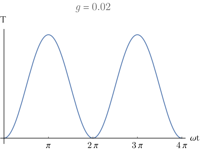
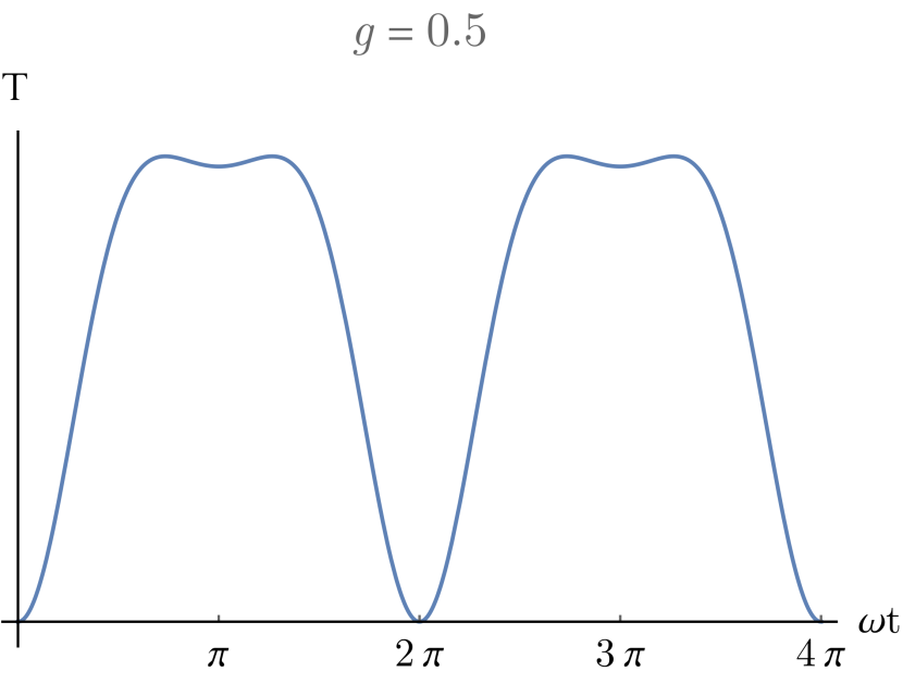
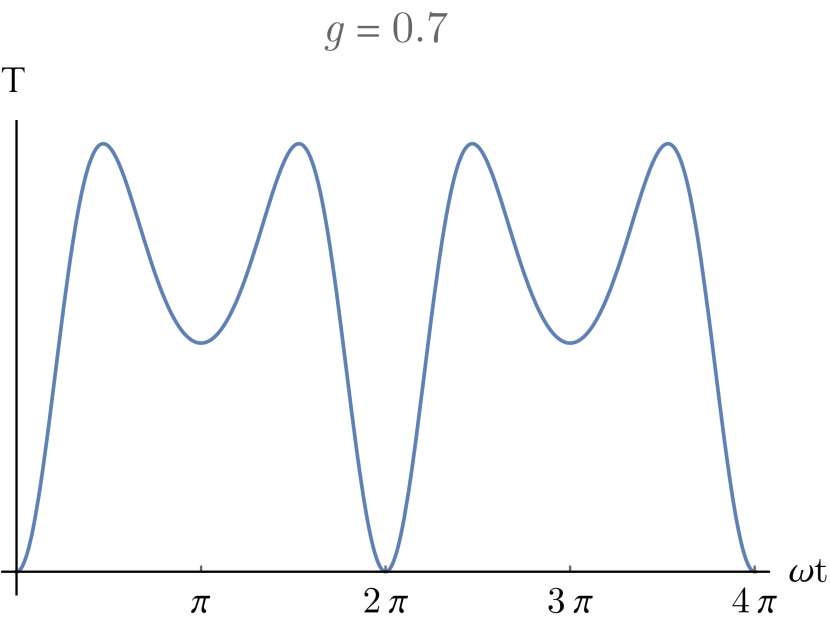
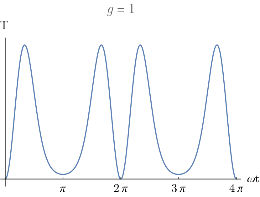
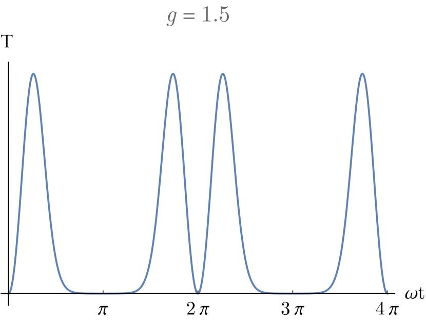
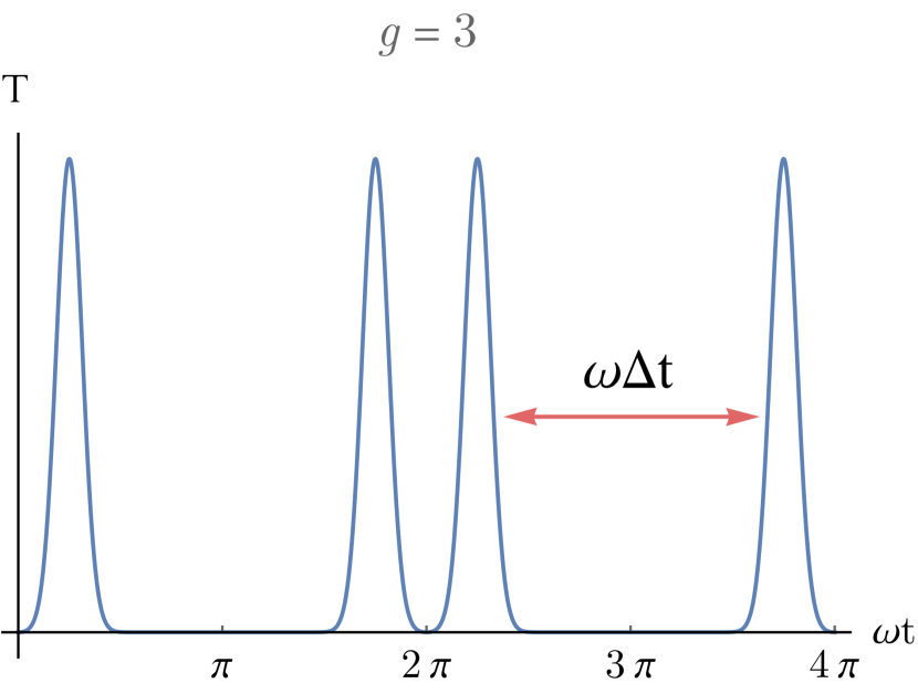
Fig. 1: Plot of ${\rm T}(t)$ for several values of the coupling $g$. The functions are normalized to $1$.

For small values of $g$ it is

$${\rm T}(t)\sim\frac{1}{2}g^{2}|\beta(t)|^{2}=\frac{g^{4}}{\omega^{2}}(1-\cos(\omega t))\,;$$ (60)

however, as $g\to\infty$, the interval of time $\Delta t$ during which the function T$(t)$ is approximately zero, grows larger and larger in proportion to its period. This can be seen in Fig.1 and it means that there are large intervals of time during which T$(t)\approx 0$ and the system evolves unitarily under the effective hamiltonian $H_{\rm eff}$, which, we recall, is the free hamiltonian of a qubit in an external time-dependent magnetic field.

In other words, in the strong coupling regime $g\to\infty$, there is no decoherence and the qubit evolves as if it were a closed system, under the influence of an effective hamiltonian containing a time-dependent field.

4.2. Jaynes-Cummings Model

Let us now consider another model for a qubit in a bosonic environment, namely the Jaynes-Cummings model. This model is defined by the hamiltonian

$$H=\mathbb{1}\otimes\omega a^{\dagger}a+g(\sigma^{+}\otimes a+\sigma^{-}\otimes a^{\dagger})=H_{\Xi}+H_{int}~{},$$ (61)

where

$$\quad H_{\Xi}=\omega a^{\dagger}a\,,\quad H_{int}=g\left(\sigma^{+}\otimes a+\sigma^{-}\otimes a^{\dagger}\right)~{}.$$ (62)

The operators acting on $\Gamma$, $\sigma^{+}$ and $\sigma^{-}$, do not commute with each others: therefore $H_{int}$ does not describe a pure-dephasing interaction. The proper ECS are still the Glauber coherent states, while the operators $H(\alpha)$, acting on $\Gamma$, read

$$H(\alpha)=\bra{\alpha}H\ket{\alpha}=\omega|\alpha|^{2}\mathbb{1}+g(\alpha\sigma^{+}+\alpha^{*}\sigma^{-})\,,$$ (63)

and we can write

$$\frac{\partial H(\alpha)}{\partial\alpha^{*}}=g\sigma^{-}+\omega\alpha\mathbb{1}\,,\qquad\frac{\partial H(\alpha)}{\partial\alpha}=g\sigma^{+}+\omega\alpha^{*}\mathbb{1}\,;$$ (64)

therefore, the objects $\ket{\smash{\dot{\alpha}}}=D(\dot{\alpha})$ are obtained as

$$D(\dot{\alpha})=\exp[-i(g\sigma^{-}+\omega\alpha\mathbb{1})\otimes a^{\dagger}-i(g\sigma^{+}+\omega\alpha^{*}\mathbb{1})\otimes a\Big{]}$$ (65)

$$=\exp[-ig(\sigma^{+}\otimes a+\sigma^{-}\otimes a^{\dagger})-i\omega\mathbb{1}\otimes(\alpha^{*}a+\alpha a^{\dagger})\Big{]}~{}.$$

To get the operators $F_{\pm},F_{\pm}^{\dagger}$, we need to explicitly write the action of $D(\dot{\alpha})$ on $\ket{0}$. On the other hand, the presence of the non-commuting operators $\sigma^{+}$ and $\sigma^{-}$ (in contrast with the previous case, where we only had to deal with $\sigma_{z}$), makes it more difficult to factorize $D(\dot{\alpha})$ as a product of exponentials. Therefore, at variance with the pure-dephasing case, we here consider the classical limit of the environment right from the beginning, just to factorize $D(\dot{\alpha})$. In fact, it can be shown[26, 28] that

$$D(\dot{\alpha})\ket{0}\to e^{-ig\sigma^{-}\otimes a^{\dagger}}e^{-i\omega\alpha\mathbb{1}\otimes a^{\dagger}}\ket{0}~{},$$ (66)

and hence Eq. (22) reads

$$\dot{\rho}_{\Gamma}=-i\big{[}H_{\rm eff},\rho_{\Gamma}\big{]}+\int d\mu\,{\rm T}\,\Big{(}\sigma^{+}R\sigma^{-}-\frac{1}{2}\big{\{}\sigma^{-}\sigma^{+},R\big{\}}\Big{)},$$ (67)

where

$${\rm T}=2g^{2}\sum_{k}\gamma_{k}|v_{k}|^{2}\,,$$ (68)

$$H_{\rm eff}=-g\sum_{k}\int d\mu\,\gamma_{k}\Big{[}\imaginary(v_{k}u^{*}_{k})\sigma_{x}+\real(v_{k}u^{*}_{k})\sigma_{y}\Big{]}\,,$$

and $v_{k},u_{k}$ are functions on the manifold. Getting their expression would be the same as solving the exact quantum dynamics of the system and its enviroment, altogether, which is not an achievable task. However, reminding Eq. (32), when the environment becomes macroscopic and behaves classicaly we get

$$\dot{\rho}_{\Gamma}\approx-i[\tilde{H}_{\rm eff},\rho_{\Gamma}]+\widetilde{\rm T}\Big{(}\sigma^{+}\rho_{\Gamma}\sigma^{-}-\frac{1}{2}\big{\{}\sigma^{-}\sigma^{+},\rho_{\Gamma}\big{\}}\Big{)}$$ (69)

for some $\widetilde{H}_{\rm eff}$ and $\widetilde{\rm T}$ that depend neither on $\alpha$ nor on $t$, which makes the above equation (69) the well known master equation for the Jaynes-Cummings model.

5. Conclusions

In this work we have i) considered the reduced density operator for an OQS, ii) written its parametric representation with environmental coherent states, and iii) shown that its time derivative satisfies an equation that can be cast into a GKSL form, once some assumptions are made.

In particular, we have shown that it is the time derivative of the distribution $\chi^{2}(\Omega(t))$, representing the probability for the environment to be in the ECS labelled by the parameter $\Omega(t)$, that generates a GKSL structure. Moreover, the operators $F_{k},F_{k}^{\dagger}$ that we recognize as the siblings of the usual lindbladians, are defined locally on the manifold $\mathcal{M}$, that is, every $\Omega\in\mathcal{M}$ has associated to it a set of lindbladians $\{F_{k}(\Omega)\}$ entering the equation for $\dot{\rho}(t)$. Such operators depend on the microscopic details of the theory and, in principle, can be computed explicitly once the total hamiltonian of the composite system is given. Clearly, this is a highly non-trivial task, and can only be done in some specific cases. Let us finally underline that the use of ECS in our approach is crucial, as continuous parametric representations are not generally equipped with some inherent dynamics on the manifold, in the way ECS are. The possibility of associating a time evolution $\Omega(t)$ to environmental states $\ket{\Omega}$ stems from the fact that the dynamics of coherent states is known, and it is of classical type, with a classical-like hamiltonian function that is related to the original hamiltonian operator. This provides an interpretation that proves itself appropriate to obtain a GKSL general structure, and motivates further investigation along these lines, as well as comparison with related recent works, such as Refs. [33, 34, 35].

References

- [1] Eitan Ben Av, Yotam Shapira, Nitzan Akerman, and Roee Ozeri. Direct reconstruction of the quantum-master-equation dynamics of a trapped-ion qubit. Phys. Rev. A, 101:062305, Jun 2020.
- [2] Gabriel O. Samach, Ami Greene, Johannes Borregaard, Matthias Christandl, Joseph Barreto, David K. Kim, Christopher M. McNally, Alexander Melville, Bethany M. Niedzielski, Youngkyu Sung, Danna Rosenberg, Mollie E. Schwartz, Jonilyn L. Yoder, Terry P. Orlando, Joel I-Jan Wang, Simon Gustavsson, Morten Kjaergaard, and William D. Oliver. Lindblad tomography of a superconducting quantum processor, 2021.
- [3] Haimeng Zhang, Bibek Pokharel, E.M. Levenson-Falk, and Daniel Lidar. Predicting non-markovian superconducting-qubit dynamics from tomographic reconstruction. Phys. Rev. Applied, 17:054018, May 2022.
- [4] G. Passarelli, R. Fazio, and P. Lucignano. Optimal quantum annealing: A variational shortcut-to-adiabaticity approach. Phys. Rev. A, 105:022618, Feb 2022.
- [5] U. Weiss. Quantum Dissipative Systems. Series in modern condensed matter physics. World Scientific, 1999.
- [6] H. P. Breuer and F. Petruccione. The theory of open quantum systems. Oxford University Press, 2002.
- [7] G. Benenti, G. Casati, and G. Strini. Principles of Quantum Computation and Information, Volume I: basic concepts. World Scientific, 2004.
- [8] Á. Rivas and S.F. Huelga. Open Quantum Sytems: an introduction. Springer Berlin Heidelberg, 2011.
- [9] M.A. Schlosshauer. Decoherence: And the Quantum-To-Classical Transition. The Frontiers Collection. Springer, 2007.
- [10] V. Gorini, A. Kossakowski, and E.C.G. Sudarshan. Completely positive dynamical semigroups of level systems. Journal of mathematical physics, 17(5), 1976.
- [11] G. Lindblad. On the generators of quantum dynamical semigroups. Communications in mathematical physics, 48(2), 1976.
- [12] D. Chruściński and S. Pascazio. A brief history of the GKLS equation. Open Systems & Information Dynamics, 24, 2017.
- [13] S. Nakajima. On quantum theory of transport phenomena. Progress of Theoretical Physics, 20(6), 1958.
- [14] R. Zwanzig. Ensemble methods in the theory of irreversibility. Journal of Chemical Physics, 33(5), 1960.
- [15] A.O. Caldeira and A.J. Leggett. Path integral approach to quantum brownian motion. Physica A: Statistical Mechanics and its Applications, 121(3):587–616, 1983.
- [16] N. Boulant, T. F. Havel, M. A. Pravia, and D. G. Cory. Robust method for estimating the lindblad operators of a dissipative quantum process from measurements of the density operator at multiple time points. Phys. Rev. A, 67:042322, Apr 2003.
- [17] Marius de Leeuw, Chiara Paletta, and Balázs Pozsgay. Constructing integrable lindblad superoperators. Phys. Rev. Lett., 126:240403, Jun 2021.
- [18] A. McDonald and A. A. Clerk. Exact solutions of interacting dissipative systems via weak symmetries. Phys. Rev. Lett., 128:033602, Jan 2022.
- [19] W.M. Zhang, D.H. Feng, and R. Gilmore. Coherent states: Theory and some applications. Rev. Mod. Phys., 62, 1990.
- [20] A. Perelomov. Coherent states for arbitrary Lie groups. Communications in Mathematical Physics, 26(3), 1972.
- [21] A. Perelomov. Generalized Coherent States and Their Applications. Springer-Verlag Berlin Heidelberg, 1986.
- [22] L. G. Yaffe. Large- limits as classical mechanics. Rev. Mod. Phys., 54:407–435, 1982.
- [23] A. Coppo, A. Cuccoli, C. Foti, and P. Verrucchi. From a quantum theory to a classical one. Soft Computing, 24:10315, 2020.
- [24] D. Calvani, A. Cuccoli, N. I. Gidopoulos, and P. Verrucchi. Parametric representation of open quantum systems and cross-over from quantum to classical environment. Proceedings of the National Academy of Sciences, 110(17), 2013.
- [25] T. S. Cubitt, J. Eisert, and M. M. Wolf. The complexity of relating quantum channels to master equations. Communications in Mathematical Physics, 310, 2009.
- [26] C. Foti, A. Cuccoli, and P. Verrucchi. Quantum dynamics of a macroscopic magnet operating as an environment of a mechanical oscillator. Physical Review A, 94, 2016.
- [27] D. Calvani, A. Cuccoli, N. I. Gidopoulos, and P. Verrucchi. Dynamics of open quantum systems using parametric representation with coherent states. Open Syst. Inform. Dynam., 20(3), 2013.
- [28] C. Foti. On the macroscopic limit of quantum systems. PhD thesis, Università degli Studi di Firenze, 2019.
- [29] J. Lee. Introduction to Smooth Manifolds. Springer, 2012.
- [30] C. Foti, T. Heinosaari, S. Maniscalco, and P. Verrucchi. Whenever a quantum environment emerges as a classical system, it behaves like a measuring apparatus. Quantum, 3:179, 2019.
- [31] C. Foti. Dynamics of an open quantum system and effective evolution of its environment. Master’s thesis, Università degli Studi di Firenze, 2015.
- [32] G. Spaventa. Nature and origin of the operators entering the master equation of an open quantum system. Master’s thesis, Università degli Studi di Firenze, 2019.
- [33] Victor V. Albert, Barry Bradlyn, Martin Fraas, and Liang Jiang. Geometry and response of lindbladians. Phys. Rev. X, 6:041031, Nov 2016.
- [34] Sergey Denisov, Tetyana Laptyeva, Wojciech Tarnowski, Dariusz Chruściński, and Karol Życzkowski. Universal spectra of random lindblad operators. Phys. Rev. Lett., 123:140403, Oct 2019.
- [35] Moein Malekakhlagh, Easwar Magesan, and Luke C. G. Govia. Time-dependent schrieffer-wolff-lindblad perturbation theory: measurement-induced dephasing and second-order stark shift in dispersive readout. 2022.