IFIC/22-25
WUB/22-00
DESY-22-051
CERN-TH-2022-015
HU-EP-22/04
Determination of $\alpha_{s}(m_{Z})$ by the non-perturbative decoupling method

Abstract

We present the details and first results of a new strategy for the determination of $\alpha_{s}(m_{Z})$ [1]. By simultaneously decoupling 3 fictitious heavy quarks we establish a relation between the $\Lambda$-parameters of three-flavor QCD and pure gauge theory. Very precise recent results in the pure gauge theory [2, 3] can thus be leveraged to obtain the three-flavour $\Lambda$-parameter in units of a common decoupling scale. Connecting this scale to hadronic physics in 3-flavour QCD leads to our result in physical units, $\Lambda^{(3)}_{\overline{\rm MS}}=336(12)\,{\rm MeV}$, which translates to $\alpha_{s}(m_{Z})=0.11823(84)$. This is compatible with both the FLAG average [4] and the previous ALPHA result [5], with a comparable, yet still statistics dominated, error. This constitutes a highly non-trivial check, as the decoupling strategy is conceptually very different from the 3-flavour QCD step-scaling method, and so are their systematic errors. These include the uncertainties of the combined decoupling and continuum limits, which we discuss in some detail. We also quantify the correlation between both results, due to some common elements, such as the scale determination in physical units and the definition of the energy scale where we apply decoupling.

1 Introduction

Experiments in high energy physics have established the Standard Model as a very good effective theory for elementary particle physics up to the TeV scale. Consequently, the discovery of new physics will require excellent quantitative control over Standard Model (SM) predictions including QCD effects [6]. In particular, for the strong coupling, $\alpha_{s}(m_{Z})$, as one of the fundamental Standard Model parameters, a sub percent uncertainty will be required, which is significantly less than the current error for the PDG (non-lattice) average $\alpha_{s}(m_{Z})=0.1176(11)$ [7].

At present, the most accurate results for $\alpha_{s}$ are obtained from lattice QCD, as illustrated by the FLAG 2019 average $\alpha_{s}(m_{Z})=0.1182(8)$ [8], which was recently updated to $0.1184(8)$ for FLAG 2021 [4]. While lattice QCD does not require any model assumptions on hadronization, the determination of $\alpha_{s}(m_{Z})$ requires the solution of a multiscale or “window” problem (for an introduction cf. [9, 10]). Therefore, most lattice studies attempt to extract the coupling at relatively low energy scales where perturbative truncation effects are hard to control. In particular, there is now some evidence that error estimates obtained within perturbation theory can be rather misleading unless large energy scales are reached non-perturbatively [11, 12]. As a result many lattice determinations of $\alpha_{s}$ are now limited by systematic errors. cf. [9, 4].

A solution to this multiscale problem has been known for 30 years in the form of the recursive step-scaling method [13]. The method has since been applied to the running of the coupling in QCD with $N_{\mathrm{f}}=0$ [14, 2, 3, 15], $N_{\mathrm{f}}=2$ [16, 17], $N_{\mathrm{f}}=3$ [18, 5] and $N_{\mathrm{f}}=4$ [19, 20] quark flavours (for a review cf. [21]), and in various candidate models of physics beyond the Standard Model (for reviews, cf. [22, 23]). Its most recent application in 3-flavour QCD has allowed the ALPHA collaboration to non-perturbatively trace the scale evolution of the coupling in 3-flavour QCD between $0.2$ and $128$ GeV [5]. The corresponding result obtained for $\alpha_{s}(m_{Z})=0.11852(84)$ in 5-flavour QCD defines a benchmark against which to measure progress. Knowing the scale dependence of the coupling is a pre-requisite for the step-scaling solution of other renormalization problems. This is illustrated by a recent step-scaling study of the running quark mass in 3-flavour QCD [24, 25] which will provide essential input for this paper.

Current lattice QCD simulations include the light up, down and strange quarks ($N_{\mathrm{f}}=2+1$), and sometimes also the much heavier charm quark as active degrees of freedom ($N_{\mathrm{f}}=2+1+1$). The Applequist-Carazzone decoupling theorem [26] ensures that the effects of heavy sea quarks on low energy observables can be absorbed in parameter renormalizations up to effects that are power suppressed in the heavy quark masses [27]. In ref. [28] the perturbative treatment of decoupling, known to 4-loops in the $\overline{\rm MS}$ scheme [29, 30, 31, 32, 33, 34], was shown to provide an excellent quantitative description of decoupling, even at scales as low as the charm quark mass. Hence, perturbative matching of the $N_{\mathrm{f}}=3$ coupling across the charm and bottom quark thresholds yields a reliable estimate of the $N_{\mathrm{f}}=5$ coupling $\alpha_{s}(m_{Z})$ in terms of the 3-flavour $\Lambda$-parameter. The corresponding error is small and will remain sub-dominant for the foreseeable future.

The high accuracy of perturbative decoupling means that the inclusion of the charm quark is not required for a lattice determination of $\alpha_{s}(m_{Z})$. There is much more to gain from focusing on a reliable and precise determination of $\Lambda_{\rm\overline{MS\kern-0.35002pt}\kern 0.35002pt}^{(3)}$. The currently best lattice result by the ALPHA collaboration, $341(12)$ MeV, has an error of $3.5\%$ [5]. For comparison, the recent high precision study in the pure gauge theory [2] quotes $\Lambda_{\rm\overline{MS\kern-0.35002pt}\kern 0.35002pt}^{(0)}\sqrt{8t_{0}}=0.6227(98)$ i.e. an error of $1.6\%$. Given that the error due the physical scale setting is subdominant, it is thus conceivable that a substantial error reduction for $\Lambda_{\rm\overline{MS\kern-0.35002pt}\kern 0.35002pt}^{(3)}$ can still be achieved by pushing the 3-flavour step-scaling method to higher precision. While such a project would be very interesting, we emphasize that it is just as important to corroborate results with a different method.

The decoupling project, introduced in [1] and reviewed in [10], aims to deliver on both counts. It uses decoupling as a tool to connect $N_{\mathrm{f}}=3$ QCD to $N_{\mathrm{f}}=0$ QCD, and thus leverage the higher precision that can be achieved with step-scaling methods in the $N_{\mathrm{f}}=0$ theory [2, 3]. This connection is achieved by varying the RGI mass $M$ of a fictitious triplet of mass-degenerate quarks compared to a hadronic scale $\mu_{\mathrm{dec}}\approx 800$ MeV. We call this low energy scale the decoupling scale. Reaching values for $M$ of up to O($10$) GeV and using perturbative 4-loop decoupling then establishes a relation for $\Lambda_{\rm\overline{MS\kern-0.35002pt}\kern 0.35002pt}^{(N_{\mathrm{f}})}/\mu_{\mathrm{dec}}$ between both theories, with corrections that are either perturbative in the $\overline{\rm MS}$-coupling at the scale of the heavy quark mass, $M$, or power suppressed in $1/M$. Obviously, the heavy quark mass defines another scale and thus creates a potentially difficult multi-scale problem. To alleviate this problem, the choice of $\mu_{\mathrm{dec}}$ somewhat above $\Lambda_{\text{QCD}}$ is convenient, since the matching to a hadronic scale can be safely performed in a separate computation. The use of a finite volume renormalization scheme for the coupling at scale $\mu_{\mathrm{dec}}=1/L$ then reduces the decoupling project to a problem involving two physical scales, $\mu_{\mathrm{dec}}$ and $M$, where the challenge remains to reach large $z=M/\mu_{\mathrm{dec}}\gg 1$ while keeping the lattice spacing small enough so that $M\ll 1/a$. In this paper we discuss the details of the decoupling strategy and the numerical simulations we performed. When combined with earlier scale setting results [35] and precision $N_{\mathrm{f}}=0$ studies  [2, 3], the very accurate result, $\Lambda_{\rm\overline{MS\kern-0.35002pt}\kern 0.35002pt}^{(3)}=336(12)$ MeV, is obtained with uncertainties still dominated by statistical errors. Relying on the usual perturbative matching to 5-flavour QCD this translates to our result $\alpha_{s}(m_{Z})=0.11823(84)$.

The paper is organized as follows. In Section 2 we give a step by step overview of the decoupling strategy, in a language aimed also at non-lattice experts. Section 3 proposes a closer look at the continuum and decoupling limits. In particular, the leading corrections are derived in order to guide the analysis of the numerical data. Section 4 starts with the chosen set-up of non-perturbatively O($a$) improved lattice QCD with Wilson quarks, continues with a summary of the simulations with massive quarks and then presents the continuum and heavy mass extrapolations of the data which lead to the $\Lambda$-parameter. In Section 5 we obtain the corresponding result for $\alpha_{s}(m_{Z})$ and we conclude with an outlook (Section 6). A number of appendices have been included. Appendix A explains how we estimated heavy mass effects of order $1/M$ originating from the space-time boundaries. Appendix B summarizes the required $N_{\mathrm{f}}=0$ results, obtained either by dedicated $N_{\mathrm{f}}=0$ simulations or taken from the literature. Appendix C contains details about $N_{\mathrm{f}}=3$ simulations, both with massive and massless quarks. The latter are required to ensure O($a$) improvement of the renormalized quark masses. Appendix D discusses the derivation and numerical implementation of formulas (4.58) and (4.62), which allow us to perform shifts to the data and correct for small mistunings to the relevant lines of constant physics. The ingredients for quark mass renormalization and O($a$) improvement, as well as some consistency checks, are then given in Appendix E. The impact of errors in the quark mass determination is discussed in Appendix F. Finally, Appendix G explains how bare parameters were chosen on the larger lattices to ensure constant physical conditions.

2 The decoupling strategy

The decoupling strategy has been introduced and explained in ref. [1]. We assume the reader to be familiar with this reference and try to keep the overlap minimal. Some aspects of the chosen strategy may not seem obvious at first sight, as they are conditioned by previous projects of the ALPHA collaboration [36, 5, 35, 24, 2, 3]. Besides the lattice action, this concerns the choice of boundary conditions and renormalized couplings. Further technical issues arise from the necessity of O($a$) improvement and the need to control boundary effects both at O($a$) and in the heavy mass expansion. We will address these points in the following sections. Here we use a continuum language to discuss how the decoupling strategy is set up in principle.

2.1 Renormalization group invariant parameters

To set the stage we consider continuum QCD with $N_{\mathrm{f}}$ mass-degenerate quarks. The theory only has two bare parameters, the coupling and the quark mass. If these are renormalized in a mass-independent scheme $s$, their scale dependence gives rise to the definition of the $\beta$-function

$$\frac{\partial\bar{g}_{s}(\mu)}{\partial\ln\mu}=\beta_{s}(\bar{g}_{s})\raisebox{-0.43057pt}{ $\stackrel{{\scriptstyle\small{\bar{g}_{s}\to 0}}}{{\sim}}$}-\bar{g}_{s}^{3}\sum_{n\geq 0}b_{n}\bar{g}_{s}^{2n}$$ (2.1)

and the quark mass anomalous dimension,

$$\frac{\partial\ln\bar{m}_{s}(\mu)}{\partial\ln\mu}=\tau_{s}(\bar{g}_{s})\raisebox{-0.43057pt}{ $\stackrel{{\scriptstyle\small{\bar{g}_{s}\to 0}}}{{\sim}}$}-\bar{g}_{s}^{2}\sum_{n\geq 0}d_{n}\bar{g}_{s}^{2n}\,.$$ (2.2)

The renormalization scheme dependence begins with $b_{2}$ and $d_{1}$, and the universal first coefficients are, for 3 colours,

$$b_{0}=\left(11-\frac{2}{3}N_{\mathrm{f}}\right)\times(4\pi)^{-2},\quad b_{1}=\left(102-\frac{38}{3}N_{\mathrm{f}}\right)\times(4\pi)^{-4},\quad d_{0}=8\times(4\pi)^{-2}\,.$$ (2.3)

Given a non-perturbative definition of the running parameters in a scheme $s$ and thus non-perturbative results for the RG functions $\beta_{s}$ and $\tau_{s}$, one may define the renormalization group invariant (RGI) parameters,

$$\Lambda_{s} = \mu\varphi_{s}(\bar{g}_{s}(\mu))\,,$$ (2.4)

$$\varphi_{s}(\bar{g}_{s}) = (b_{0}\bar{g}_{s}^{2})^{-b_{1}/(2b_{0}^{2})}{\rm e}^{-1/(2b_{0}\bar{g}_{s}^{2})}\times\exp\left\{-\int\limits_{0}^{\bar{g}_{s}}{\rm d}x\ \left[\frac{1}{\beta_{s}(x)}+\frac{1}{b_{0}x^{3}}-\frac{b_{1}}{b_{0}^{2}x}\right]\right\}\,,$$

$$M = \overline{m}_{s}(\mu)\left[2b_{0}\bar{g}_{s}^{2}(\mu)\right]^{-\frac{d_{0}}{2b_{0}}}\exp\left\{-\int\limits_{0}^{\bar{g}_{s}(\mu)}\left[\frac{\tau_{s}(x)}{\beta_{s}(x)}-\frac{d_{0}}{b_{0}x}\right]\,dx\right\}\,,$$ (2.5)

where the RGI quark mass $M$ is scheme independent, while $\Lambda_{s}$ depends on the renormalization scheme $s$, the standard reference being the $\overline{\rm MS}$ scheme of dimensional regularization. The running coupling, the quark mass, and the RGI parameters are defined for QCD with a fixed flavour number $N_{\mathrm{f}}$. We occasionally indicate this dependence by a superscript; when omitted we refer to QCD with non zero $N_{\mathrm{f}}$ implying $N_{\mathrm{f}}=3$ in our numerical work. Note that the ratio $\Lambda_{s}/\mu$ is, for large enough $\mu$, in one-to-one correspondence with the coupling $\bar{g}_{s}^{2}(\mu)$ in scheme $s$. Hence, the running parameters in scheme $s$ at large $\mu$ can be traded for $\Lambda_{{\rm\overline{MS\kern-0.35002pt}\kern 0.35002pt}}/\mu$ and the scheme independent RGI quark mass $M$.

2.2 Decoupling relations

So far we have assumed that the coupling and quark mass are renormalized in a mass-independent scheme. In practice, this is achieved by imposing the renormalization condition at vanishing quark mass [37]. A renormalized coupling at finite quark mass defines a function $\bar{g}_{s}(\mu,M)$ such that, for $M\ll\mu$, it coincides with the coupling in a massless scheme, $\bar{g}_{s}(\mu,0)=\bar{g}_{s}(\mu)$, whereas, for $M\gg\mu$ its scale dependence is well described by an effective theory with the $N_{\mathrm{f}}$ heavy quarks removed. In the absence of other light quarks, this simply is the pure gauge theory or “quenched ($N_{\mathrm{f}}=0$) QCD”. We can thus write

$$\bar{g}_{s}(\mu,M)=\bar{g}_{s}^{(0)}(\mu)+{\rm O}(\mu^{2}/M^{2})\,,$$ (2.6)

where on the r.h.s. the scale $\mu$ in units of the pure gauge theory $\Lambda$-parameter has an implicit $M$-dependence. The mass-dependent coupling is thus seen to interpolate the couplings in QCD with $N_{\mathrm{f}}$ and zero flavours. This in turn implies a relation between the respective mass independent couplings. In perturbation theory and in the $\overline{\rm MS}$ scheme the ensuing relations have been computed up to 4-loop order [29, 30, 31, 32, 33, 34]:

$$[\bar{g}^{(0)}_{\rm\overline{MS\kern-0.35002pt}\kern 0.35002pt}(\mu)]^{2}=C(\bar{g}_{{\rm\overline{MS\kern-0.35002pt}\kern 0.35002pt}}(m_{\star}))\bar{g}^{2}_{{\rm\overline{MS\kern-0.35002pt}\kern 0.35002pt}}(m_{\star})$$ (2.7)

where the scale choice $\mu=m_{\star}=\overline{m}_{{\rm\overline{MS\kern-0.35002pt}\kern 0.35002pt}}(m_{\star})$ eliminates the 1-loop coefficient in

$$C(x)=1+c_{2}x^{4}+c_{3}x^{6}+c_{4}x^{8}+\ldots\,,$$ (2.8)

and, for $N_{\mathrm{f}}=3$, one obtains [34]

$$c_{2}=2.940776\times 10^{-4},\qquad c_{3}=4.435355\times 10^{-5},\qquad c_{4}=5.713208\times 10^{-6}\,.$$ (2.9)

Beyond perturbation theory, the limit of infinite $M/\mu$ requires the extrapolation of numerical data and one would like to understand how it is approached. To this end, the language of effective field theory is most helpful, cf. [28]. Assuming that the heavy quark limit is described by a local effective theory, one obtains a systematic expansion in inverse powers of the quark mass $M$. In particular, with all fermions decoupled simultaneously the effective theory takes the form of the pure gauge theory where the inverse mass corrections are proportional to insertions of higher dimensional local gluonic operators. One naturally wonders whether all powers of $1/M$ may appear in this expansion. In the absence of space-time boundaries, and for gluonic observables defining the running couplings, the locality of the effective decoupling theory, Euclidean O(4) symmetry and gauge invariance rule out any odd-dimensional terms so that the expansion is effectively in $1/M^{2}$.

The situation changes if space-time is a manifold with boundaries, as this allows for additional local boundary terms at order $1/M$ in the effective Lagrangian. This is relevant in our case, where we use the standard Schrödinger functional set-up on a space-time hyper-cylinder of 4-volume $L^{3}\times T$, with Dirichlet boundary conditions imposed on some of the fermionic and gauge field components at Euclidean times $x_{0}=0$ and $x_{0}=T$ [38, 39]. In order to minimize the impact of such boundary contributions, we chose a geometry such as to have large distances from the boundary to the observable defining the coupling in the mass-dependent scheme. Using the decoupling effective field theory, with a single local term at the boundaries $x_{0}=0$ and $x_{0}=T$, we are able to compute the $1/M$ contributions to the coupling. They are given in terms of a 1-loop matching coefficient (see section A.1) and a non-perturbative matrix element. The latter is evaluated by simulations in the decoupled theory with $N_{\mathrm{f}}=0$ and extrapolated to the continuum (see section A.2). We can thus confirm that the boundary effects are negligible for $T=2L$.

2.3 Master formula and strategy breakdown

Following Ref. [1], the decoupling strategy can be cast in the form

$$\frac{\Lambda_{{\rm\overline{MS\kern-0.35002pt}\kern 0.35002pt}}}{\mu_{\mathrm{dec}}}=\frac{\Lambda_{\rm\overline{MS\kern-0.35002pt}\kern 0.35002pt}^{(0)}}{\Lambda_{s}^{(0)}}\times\lim_{M/\mu_{\mathrm{dec}}\rightarrow\infty}\left[\dfrac{\varphi_{s}^{(0)}\left(\bar{g}_{s}(\mu_{\mathrm{dec}},M)\right)}{P\left(\frac{M}{\mu_{\mathrm{dec}}}\left/\frac{\Lambda_{{\rm\overline{MS\kern-0.25002pt}\kern 0.25002pt}}}{\mu_{\mathrm{dec}}}\right.\right)}\right]\,.$$

(2.10)

Note that the desired ratio $\Lambda_{{\rm\overline{MS\kern-0.35002pt}\kern 0.35002pt}}/\mu_{\mathrm{dec}}$ on the l.h.s. in $N_{\mathrm{f}}=3$ QCD also appears on the r.h.s. in the argument of the function $P$, i.e the equation is implicit. In order to solve it one needs to be able to both evaluate the pure gauge theory function $\varphi_{s}^{(0)}$ and the function $P$. The latter corresponds to $P_{0,N_{\mathrm{f}}}$ in the notation of [28], where it was shown that non-perturbatively $P$ has an ambiguity of order $(\Lambda/M)^{2}$, which arises once the reference to a specific matching condition is removed. A major result of [28] is the observation that the perturbative evaluation of $P$ using the ${\rm\overline{MS\kern-0.50003pt}\kern 0.50003pt}$-scheme is numerically very accurate already for quark masses in the charm region. With the heavy quark mass setting the scale for the ${\rm\overline{MS\kern-0.50003pt}\kern 0.50003pt}$-coupling, the accuracy further improves towards the decoupling limit. In practice, Eq. (2.10) will be used for a range of finite but reasonably large values $M/\mu_{\mathrm{dec}}$. When using a perturbative approximation for $P$ in the $\overline{\rm MS}$ scheme, deviations from the limit are expected to be on one hand proportional to $1/M^{2}$ and on the other hand logarithmic corrections of $\text{O}(\alpha_{\overline{\rm MS}}^{4}(M))$. This assumes that linear terms in $1/M$ are either completely absent by symmetry or that they can be controlled or subtracted explicitly.

While decoupling can be studied in the infinite volume regime [28], for a lattice QCD approach it is advantageous to separate the determination of the hadronic scales from the study of decoupling, by using a finite volume renormalization scheme [1]. We use the GF scheme with SF boundary conditions, first introduced in [40], with details given in [35]. In a continuum language it is given by

$$\bar{g}^{2}_{\text{GF}}(\mu)={\cal N}^{-1}\left.\sum_{k,l=1}^{3}\dfrac{t^{2}\langle{\rm tr}\left\{G_{kl}(t,x)G_{kl}(t,x)\right\}\delta_{Q,0}\rangle}{\langle\delta_{Q,0}\rangle}\right|_{\mu=1/L,T=L,\,M=0}^{x_{0}=T/2,\,c=\sqrt{8t}/L}$$ (2.11)

where $G_{\mu\nu}(t,x)$ denotes the field tensor for the gauge field at flow time $t$, and ${\cal N}$ is a known normalization factor which ensures $\bar{g}^{2}_{\text{GF}}(\mu)=g_{0}^{2}+{\rm O}(g_{0}^{4})$, with $g_{0}$ the bare coupling. The projection onto the topological charge $Q=0$ sector is part of the scheme definition and merely introduced in order to avoid technical difficulties with the numerical simulation algorithms. The remaining parameter $c$ fixes the ratio between the scales set by the flow time and the finite volume.

We may now break down the decoupling strategy into several steps:

1. Decoupling scale $\mu_{\mathrm{dec}}$: Given the coupling in the massless fundamental theory, we fix $\mu_{\mathrm{dec}}$ by setting

   $$\bar{g}^{2}_{\text{GF}}(\mu_{\mathrm{dec}})=3.949\,.$$ (2.12)

   From previous work [35, 5] one finds $\mu_{\mathrm{dec}}=789(15)\,{\rm MeV}$, which is a typical QCD scale. Eq. (2.12) defines a so-called line of constant physics (LCP); following it towards the continuum, lattice spacing $a\to 0$, means that the limit is approached at fixed $\mu_{\mathrm{dec}}/\Lambda_{{\rm\overline{MS\kern-0.35002pt}\kern 0.35002pt}}$. Evaluating the LCP for a given lattice size $L/a=1/(a\mu_{\mathrm{dec}})$ defines a corresponding value for the bare coupling, $g_{0}^{2}\equiv 6/\beta$, and vice versa. We have implicitly assumed here that $M$ vanishes. With Wilson fermions this requires a further tuning condition on the bare mass parameter. Details are discussed in section 4.1.

2. Definition of $z=M/\mu_{\mathrm{dec}}$: A further set of constant physics conditions is obtained by fixing the RGI quark mass in units of $\mu_{\mathrm{dec}}$. Choosing a set of values in the range $\in[2,12]$, one needs to work out, for given lattice spacing (as obtained from Eq. (2.12)) the corresponding bare mass parameters $am_{0}$. The details of this procedure will be discussed in Section 4.2.

3. Determination of $\bar{g}^{(0)}_{\text{GFT}}(\mu_{\mathrm{dec}})$: The value of a renormalized coupling in the $N_{\mathrm{f}}=0$ theory, at a known scale $\mu_{\mathrm{dec}}$ is obtained by evaluating the same coupling in the fundamental theory at a heavy mass $M$ and assuming decoupling. The main problem with a mass dependent GF-coupling are boundary $1/M$ terms, which render decoupling slower than necessary. In order to minimize these effects we use a variant of the coupling with $T=2L$,

   $$\bar{g}^{2}_{\text{GFT}}(\mu,M)=\left.\bar{g}^{2}_{\text{GF}}(\mu)\right|_{T\to 2L,M\to z\mu}\,.$$ (2.13)

   Compared to the GF coupling (2.11) this doubles the distance of the magnetic energy density to the boundaries, thereby reducing the coefficient of the $1/M$ boundary contribution substantially. Calling this scheme GFT, the main computational effort was required for the evaluation of $\bar{g}^{2}_{\text{GFT}}(\mu_{\mathrm{dec}},M)$, at the lattice spacings and bare quark masses which follow from the chosen lines of constant physics.

4. Determination of $\bar{g}^{(0)}_{\text{GF}}(\mu_{\mathrm{dec}})$: Obtaining this input value for the precisely known $\varphi_{\text{s}}^{(0)}$ (with the scheme $s=\text{GF}$) in Eq. (2.10) requires the establishment of a non-perturbative relation between the GF and the GFT schemes in the $N_{\mathrm{f}}=0$ theory at scale $\mu_{\mathrm{dec}}$. This is achieved by evaluating the GF coupling along a LCP defined by a fixed value of the GFT coupling, and continuum extrapolating.

5. Determination of $\Lambda_{{\rm\overline{MS\kern-0.35002pt}\kern 0.35002pt}}^{(0)}/\mu_{\mathrm{dec}}$: The recent step-scaling study of the GF coupling in [2] allows us to evaluate $\varphi_{\text{GF}}(\bar{g}^{(0)}_{\text{GF}}(\mu_{\mathrm{dec}}))=\Lambda^{(0)}_{\text{GF}}/\mu_{\mathrm{dec}}$ which completes the numerator in the square brackets of Eq. (2.10). The conversion to the $\overline{\rm MS}$ $\Lambda$-parameter then simply requires the one-loop matching between the GF and $\overline{\rm MS}$-couplings in the pure gauge theory [41].

6. The function $P$ gives the ratios of $\Lambda$-parameters between the fundamental and effective theories and can be reliably evaluated in massless continuum perturbation theory

   $$P=\varphi^{(0)}_{{\rm\overline{MS\kern-0.35002pt}\kern 0.35002pt}}(g_{\star}\sqrt{C(g_{\star})})/\varphi_{{\rm\overline{MS\kern-0.35002pt}\kern 0.35002pt}}(g_{\star})\,,$$ (2.14)

   with $C(g)$ known to 4-loop order, cf. Eq. (2.9) and the notation $g_{\star}=\bar{g}_{\rm\overline{MS\kern-0.35002pt}\kern 0.35002pt}(m_{\star})$. In particular, the quark mass $M$ only enters to set the scale. For given $z=M/\mu_{\mathrm{dec}}$, the l.h.s. and the function $P$ in Eq. (2.10) only depend on $\Lambda_{{\rm\overline{MS\kern-0.35002pt}\kern 0.35002pt}}/\mu_{\mathrm{dec}}$ and with $\varphi_{\text{GF}}$ known it remains to numerically solve for $\Lambda_{{\rm\overline{MS\kern-0.35002pt}\kern 0.35002pt}}/\mu_{\mathrm{dec}}$. This is to be repeated for all available $z$-values and the result for $\Lambda_{{\rm\overline{MS\kern-0.35002pt}\kern 0.35002pt}}/\mu_{\mathrm{dec}}$ is then obtained by extrapolation to the decoupling limit.

Concluding this overview, we see that, besides the evaluation of the GFT coupling in a mass-dependent scheme, the main ingredients are precision results in the pure gauge theory for the running GF coupling and the matching between GF and GFT schemes. Together with available 5-loop perturbative results for the function $P$, this allows us to infer the $N_{\mathrm{f}}=3$ $\Lambda$-parameter in units of $\mu_{\mathrm{dec}}$ and thus in MeV, given the relation of $\mu_{\mathrm{dec}}$ to a hadronic scale from [35].

3 The continuum and decoupling limits: a closer look

In this section we discuss the approach to the continuum and decoupling limits in some more detail, in order to provide the theoretical underpinning for the analysis of the lattice data. While the limits are conceptually independent, in practice they are best dealt with together, in terms of effective continuum field theories. The methods of refs. [42, 43, 44, 45, 46] allow us in principle to go beyond power law behaviour and use renormalization group improved perturbation theory to obtain the correct leading asymptotics. This holds true for both limits, with the small parameter being either the lattice spacing or the inverse quark mass. While the information for the bulk effects is still incomplete, the discussion serves to motivate the fit ansätze which will be used in the data analysis, cf. Section 4. For the boundary $1/m$ effects we are able to estimate the full contribution in Section 3.3 without a fit to the data. We will focus on the bulk effects first and address the influence of the boundaries in the Euclidean time direction in the end.

3.1 Symanzik’s effective theory for lattice QCD

Following Symanzik [47, 48, 49, 50], the approach of a connected lattice correlation function to the continuum limit can be described in terms of an effective continuum theory, with action

$$S_{\text{eff}}=S_{0}+aS_{1}+a^{2}S_{2}+\ldots\,.$$ (3.15)

Here, $S_{0}$ is the continuum action and $S_{k}$ are space-time integrals over linear combinations of local composite fields of mass dimension $4+k$, $k=1,2,\ldots$, which respect all the symmetries of the lattice action. We will omit $S_{1}$ in the following, assuming a non-perturbatively O($a$) improved lattice set-up. Residual effects due to $S_{1}$ are dealt with separately (cf. Sect. 3.3 and Appendix E).

Local fields $O$ defining the observables are represented by corresponding effective fields and expanded similarly,

$$O_{\text{eff}}=O_{0}+aO_{1}+a^{2}O_{2}+\ldots\,.$$ (3.16)

Gluonic gradient flow observables $O_{\text{gf}}$ can be formulated in terms of a local 4+1 dimensional field theory [51, 52] with the flow time $t$ as the extra coordinate. This allows us to work entirely in terms of local observables $O$ and improve them to O($a^{2}$), such that $O_{1}$ and $O_{2}$ vanish in the effective field description. We also assume that the O($a^{2}$) effects originating from the 4+1 dimensional bulk action are removed by an appropriate O($a^{2}$) modification of the flow equation [52]. The Symanzik expansion for such observables then takes the form

$$\langle O_{\text{gf}}\rangle_{\text{lat}}=\langle O_{\text{gf}}\rangle_{\text{cont}}-a^{2}\langle O_{\text{gf}}S_{2}\rangle_{\text{cont}}+\ldots,$$ (3.17)

in terms of connected correlation functions. Although $S_{2}$ contains an integral over space-time, no contact terms are generated for gradient flow observables $O_{\text{gf}}$, as they are separated from $S_{2}$ by the finite flow time $t$. For the lattice set-up with non-perturbatively O($a$) improved, mass degenerate Wilson quarks, $S_{2}$ is given as a linear combination of 18 local dimension-6 operators,

$$S_{2}=\int d^{4}x\,\sum_{i=1}^{18}\omega_{i}{\mathcal{O}}_{i}(x)\,,$$ (3.18)

integrated over space-time. This constitutes an operator basis after the use of the equations of motion, the elimination of total derivative terms and the use of relations among 4-quark operators due to Fierz transformations. In the absence of gradient flow observables, the equations of motion simplify and allow for the elimination of 2 operators [45].

Note that Eq. (3.17) makes the power dependence on the lattice spacing explicit. An additional $a$-dependence arises through the coefficients $\omega_{i}$ of the operators in $S_{2}$, as these can be understood as functions of a renormalized coupling at the cutoff scale, $\mu=1/a$. Close to the continuum limit asymptotic freedom implies that their leading asymptotic behaviour is exactly computable. This was first used by Balog, Niedermayer and Weisz [53, 54] in their analysis of the 2-dimensional O($n$) $\sigma$-model. The technique has recently been extended and applied to gauge theories in various lattice regularisations, including lattice QCD with quarks of both the Wilson and Ginsparg-Wilson type [42, 44, 43, 45, 46]. Technically, one needs to compute, to 1-loop order, the anomalous dimension matrix for the set of mass dimension 6 operators entering $S_{2}$. The operator basis mixes under renormalization, ${\mathcal{O}}_{\text{R},i}=\sum_{j=1}^{18}Z_{ij}{\mathcal{O}}_{j}$, and, following our conventions from Sect. 2, we define the corresponding anomalous dimension matrix

$$\gamma_{ij}^{\cal O}=\sum_{k=1}^{18}\left(\mu\dfrac{d}{d\mu}Z_{ik}\right)\left(Z^{-1}\right)_{kj}=-g^{2}\left[{(\gamma_{0}^{\cal O})}_{ij}+{(\gamma_{1}^{\cal O})}_{ij}g^{2}+{\rm O}(g^{4})\right]\,.$$ (3.19)

A change of basis, ${{\cal B}}_{i}=\sum_{j}V_{ij}{\cal O}_{j}$, may then be performed in order to diagonalize the one-loop anomalous dimension matrix, $\gamma_{0}^{\cal O}$, and determine its eigenvectors and eigenvalues. Denoting the transformed anomalous dimension matrix by

$$\gamma^{{\cal B}}=V\gamma^{\cal O}V^{-1}=-g^{2}\left(\gamma^{{\cal B}}_{0}+\gamma^{{\cal B}}_{1}g^{2}+\ldots\right),\qquad\left(\gamma_{0}^{{\cal B}}\right)_{ij}=\delta_{ij}\gamma_{0,i}^{{\cal B}}\,,$$ (3.20)

renormalization group invariant (RGI) operators can be defined through

$${{\cal B}}_{i}^{\text{RGI}}=\lim_{\mu\rightarrow\infty}\left[\alpha_{\overline{\rm MS}}(\mu)\right]^{-\hat{\gamma}_{i}^{\cal B}}{{\cal B}}_{i}(\mu)\,,\qquad\hat{\gamma}^{\cal B}_{i}=\gamma_{0,i}^{{\cal B}}/(2b_{0})\,.$$ (3.21)

At finite $\mu$ there are corrections of O($\alpha$) stemming from the two- and higher loop anomalous dimensions. Note also the $N_{\mathrm{f}}$-dependence of $\hat{\gamma}^{\cal B}_{i}$, due to the normalization by $2b_{0}$.

In terms of the eigenbasis of operators, $\{{{\cal B}}_{i}\}$, the cutoff effects take the form

$$\langle O_{\text{gf}}\rangle_{\text{lat}}=\langle O_{\text{gf}}\rangle_{\text{cont}}-a^{2}\sum_{i}b_{i}\left(\alpha_{\overline{\rm MS}}(1/a)\right)[\alpha_{\overline{\rm MS}}(1/a)]^{\hat{\gamma}^{\cal B}_{i}}\int d^{4}x\langle O_{\text{gf}}{{\cal B}}^{\text{RGI}}_{i}(x)\rangle+\ldots\,,$$ (3.22)

where the coefficient functions

$$b_{i}(\alpha)=\sum_{j=1}^{18}\omega_{j}(\alpha)\,(V^{-1})_{ji}=\sum_{n\geq 0}\alpha^{n}b_{i}^{(n)},$$ (3.23)

are given as a linear combination of the $\omega_{i}$, Eq. (3.18), and are thus perturbatively computable. For tree-level O($a^{2}$) improved lattice actions, $b^{(0)}_{i}=0$, and the higher coefficients can be successively eliminated by perturbative O($a^{2}$) improvement of the lattice action. For lattice QCD with O($a$) improved Wilson quarks, one then expects that the leading cutoff effects in the bulk are of the form

$$\langle O_{\text{gf}}\rangle_{\text{lat}} = \langle O_{\text{gf}}\rangle_{\text{cont}}-a^{2}\sum_{i=1}^{18}A_{i}[\alpha_{\overline{\rm MS}}(1/a)]^{\hat{\Gamma}_{i}}\left\{1+{\rm O}(\alpha_{\overline{\rm MS}}(1/a))\right\}+{\rm O}(a^{3})\,,$$ (3.24)

$$A_{i} = b_{i}^{(n_{i}^{\mathrm{I}})}\int d^{4}x\,\left\langle O_{\text{gf}}{{\cal B}}^{\text{RGI}}_{i}(x)\right\rangle_{\text{cont}}\,,$$ (3.25)

where the neglected powers in $\alpha$ include both the expansion of $b_{i}(\alpha)$ and terms containing the (non-diagonal) higher order anomalous dimensions. The constants $A_{i}$ contain the insertions of the scale-independent RGI operators and $\hat{\Gamma}_{i}=\hat{\gamma}^{\cal B}_{i}+n_{i}^{\mathrm{I}}$ depends on the degree of perturbative O($a^{2}$) improvement of the lattice action. For example, a tree-level (completely) improved action leads to $n_{i}^{\mathrm{I}}\geq 1$ and in general we have $b_{i}=\hat{b}_{i}\alpha^{n_{i}^{\mathrm{I}}}(1+{\rm O}(\alpha))$.

For $N_{\mathrm{f}}=3$ lattice QCD, with O($a$) improved Wilson quarks, Husung et al. [45, 44, 46] found that the spectrum for the 1-loop anomalous dimensions is bounded from below by $\hat{\Gamma}_{i}\geq-1/9$, for the basis of 16 operators needed for observables not involving the gradient flow. There are then 6 operators found with 1-loop anomalous dimensions $-1/9\leq\hat{\Gamma}_{i}<8/9$. The remaining operators describe cutoff effects accompanied by powers of $\alpha$ equal or higher than other neglected terms and may therefore be discarded. Explicit expressions for the eigen-operators of the 1-loop anomalous dimension matrix are, in general, rather complicated and will not be required here. For the case of gradient flow observables this result is not complete, as there are two further dimension 6 operators which must be included to obtain the full matrices $V$ and $\gamma^{\cal O}_{0}$ [45]. They have so far only been computed in the pure gauge theory [45].

In view of the heavy mass expansion, there is a very interesting block structure in $\gamma^{\cal O}_{0}$, for the subset of operators in $S_{2}$ which come with a positive power of the quark mass. For $N_{\mathrm{f}}=3$ with non-degenerate quarks there are eleven operators [45, 44, 46], which reduce to just three for degenerate quarks, namely

$${\mathcal{O}}_{m,1}=\frac{1}{g_{0}^{2}}\sum_{\mu,\nu}m^{2}\,\hbox{tr}\left(F_{\mu\nu}F_{\mu\nu}\right)\,,\qquad{\mathcal{O}}_{m,2}=m^{3}\overline{\psi}\psi\,,\qquad{\mathcal{O}}_{m,3}=\frac{1}{4}\sum_{\mu,\nu}m\overline{\psi}\,i\sigma_{\mu\nu}F_{\mu\nu}\psi\,.$$ (3.26)

Note that this subset will remain the same for gradient flow observables, as the additional operators do not come with mass factors. Moreover, the tridiagonal block structure of $\gamma^{\cal O}_{0}$ means that their anomalous dimensions will not be affected by enlarging the basis and their renormalization can be consistently carried out ignoring the remainder of the basis [45, 44, 46]. This is fortunate, as it means that the structure of the leading $a^{2}m^{2}$ lattice effects can be inferred with current knowledge. We denote the corresponding basis of eigen-operators for the 1-loop anomalous dimension matrix by $\{{{\cal B}}_{m,i}\}_{i=1,2,3}$, and their 1-loop anomalous dimensions are then given by [45, 44, 46],

$$\hat{\gamma}^{\cal B}_{m,1}=-1/9\,,\qquad\hat{\gamma}^{\cal B}_{m,2}=14/27\,,\qquad\hat{\gamma}^{\cal B}_{m,3}=8/9\,.$$ (3.27)

Furthermore, from [45, 44, 46] one infers that, for our lattice action (cf. Appendix C), we have ${b}_{m,i}=\hat{b}_{m,i}+{\rm O}(\alpha)$ so that $\hat{\Gamma}_{m,i}=\hat{\gamma}^{\cal B}_{m,i}$ for $i=1,2,3$. We note that one only needs to retain the first two operators as the difference $\hat{\gamma}^{\cal B}_{m,3}-\hat{\gamma}^{\cal B}_{m,1}=1$ translates to a relative factor of $\alpha$, i.e. ${{\cal B}}_{m,3}$ contributes at the same order as other neglected contributions.

3.2 The decoupling expansion

The Symanzik expansion renders the $a$-dependence explicit, both for the powers of $a$ and the leading logarithmic terms given as fractional powers of $\alpha_{\overline{\rm MS}}(1/a)$. The connected correlation functions which appear in this expansion are thus defined in the continuum limit, with respect to the continuum QCD action. In a second step, we now determine how the continuum correlation functions, $\langle O_{\text{gf}}\rangle_{\text{cont}}$, $\langle O_{\text{gf}}S_{2}\rangle_{\text{cont}},$ behave as the quark mass $m$ is taken large. The effective decoupling theory bears formal similarities with Symanzik’s effective theory, in particular it renders both the powers in $1/m$ and the logarithmic corrections explicit. The effective decoupling action can be expanded,

$$S_{\text{dec}}=S_{0,\text{dec}}+\frac{1}{m}S_{1,\text{dec}}+\frac{1}{m^{2}}S_{2,\text{dec}}+{\rm O}(1/m^{3})\,,$$ (3.28)

with

$$S_{0,\text{dec}} = -\frac{1}{2}\int d^{4}x\,{\cal D}_{0}(x)\,,\qquad{\cal D}_{0}=\frac{1}{g_{0}^{2}}\,\hbox{tr}(F_{\mu\nu}F_{\mu\nu})\,,$$ (3.29)

$$S_{2,\text{dec}} = \int d^{4}x\left(d^{\mathrm{S}}_{1}{\cal D}_{1}(x)+d^{\mathrm{S}}_{2}{\cal D}_{2}(x)\right).$$ (3.30)

Due to the simultaneous decoupling of all quarks the leading term, $S_{0,\text{dec}}$, is given by the pure gauge action. $S_{k,\text{dec}}$ are given space-time integrals of gauge invariant local operators of mass dimension $4+k$, polynomial in the gauge field and its derivatives. Gauge and $O(4)$ symmetries do not allow for odd values of $k$, so that the first order term must vanish. The dimension-6 pure gauge operators in Eq. (3.30) take the form,

$${\cal D}_{1}=\frac{1}{g_{0}^{2}}\sum_{\mu,\nu,\rho}\,\hbox{tr}\left(D_{\mu}F_{\mu\nu}D_{\rho}F_{\rho\nu}\right)\,,\qquad{\cal D}_{2}=\frac{1}{g_{0}^{2}}\sum_{\mu,\nu,\rho}\,\hbox{tr}\left(D_{\mu}F_{\rho\nu}D_{\mu}F_{\rho\nu}\right)-\frac{23}{7}{\cal D}_{1}\,,$$ (3.31)

where we have directly chosen the eigenbasis of the one-loop anomalous dimension matrix, with eigenvalues $\hat{\gamma}^{\cal D}_{0,1,2}=-1,0,7/11$, respectively. The coefficients $d^{\mathrm{S}}_{1,2}$ are matching coefficients between QCD with $N_{\mathrm{f}}=3$ heavy quarks and the $N_{\mathrm{f}}=0$ effective theory and can be perturbatively expanded in $\alpha_{\rm\overline{MS\kern-0.35002pt}\kern 0.35002pt}$, taken at the decoupling scale. In perturbation theory, this scale is most naturally defined as the running quark mass $\overline{m}_{\overline{\rm MS}}\left(\mu\right)$ at its own scale,

$$m_{\star}=\overline{m}_{\overline{\rm MS}}\left(m_{\star}\right),$$ (3.32)

which also defines the (inverse) expansion parameter of the effective decoupling theory.

Besides the effective action, observables $O$ have an effective large mass description, too. For the case of linear combinations of the fields ${\cal B}_{i}$, $O=\sum_{i}c_{i}{{\cal B}}_{i}$, it starts with a term of O($m^{2}$). We thus expect the form

$$[O]_{\text{dec}}=m^{2}\sum_{k\geq 0}\frac{1}{m^{2k}}{O_{\text{$2k$,dec}}}\,,$$ (3.33)

where the fields ${O_{\text{$2k$,dec}}}$ are linear combinations of gauge invariant local composite fields, polynomial in the gauge field and its derivatives, of mass dimension $d_{O}+2(k-1)$, where $d_{O}$ is the dimension of the observable. For gradient flow observables $O_{\text{gf}}$ we will assume that the effective observable description reduces to the term with $k=1$.

We will now look at the combined Symanzik and decoupling expansion in $a$ and $1/m$ and discuss in turn the corrections terms of order O($1/m^{2}$), O($a^{2}m^{2}$) and O($a^{2})$. We emphasize that the decoupling expansion is applied to the Symanzik effective theory. Hence, the combined expansion is valid for

$$q\ll m\ll 1/a\,,$$ (3.34)

for all scales $q$ present in the observable considered. In our application these are $q\in\{1/\sqrt{8t},\Lambda_{\mathrm{QCD}}\}$.

3.2.1 Corrections of O($1/m^{2}$)

To order $1/m^{2}$ in the heavy mass expansion, we formally have,

$$\langle O_{\text{gf}}\rangle_{\text{cont}}=\langle O_{\text{gf}}\rangle_{\text{dec}}-\frac{1}{m^{2}}\langle O_{\text{gf}}S_{2,\text{dec}}\rangle_{\text{dec}}+\ldots\,,$$ (3.35)

which evaluates to

$$\langle O_{\text{gf}}\rangle_{\text{cont}}=\langle O_{\text{gf}}\rangle_{\text{dec}}-\frac{1}{m_{\star}^{2}}\sum_{i=1}^{2}d^{\mathrm{S}}_{i}[\alpha_{{\rm\overline{MS\kern-0.35002pt}\kern 0.35002pt}}^{(0)}(m_{\star})]^{\hat{\gamma}^{\cal D}_{i}}\int d^{4}x\langle O_{\text{gf}}{\cal D}_{i}^{\text{RGI}}(x)\rangle_{\text{dec}}+\ldots\,,$$ (3.36)

where we have converted to the RGI operators in the $N_{\mathrm{f}}=0$ theory. Without performing an explicit matching calculation, the leading order, $l^{\mathrm{S}}_{i}$, in $d^{\mathrm{S}}_{i}=\hat{d}^{\rm S}_{i}\alpha^{l^{\mathrm{S}}_{i}}+{\rm O}(\alpha^{l^{\mathrm{S}}_{i}+1})$, $i=1,2$, is not known and we will have to use assumptions for $l^{\mathrm{S}}_{i}$. Also converting to the RGI quark mass, $M$,

$$m_{\star}=[8\pi b_{0}\alpha_{\rm\overline{MS\kern-0.35002pt}\kern 0.35002pt}(m_{\star})]^{\hat{\gamma}_{m}}M\,,\qquad\hat{\gamma}_{m}=4/9\quad(N_{\mathrm{f}}=3)\,,$$ (3.37)

then leads to the asymptotic large mass behaviour in the continuum limit of the form

$$\langle O_{\text{gf}}\rangle_{\text{cont}}=\langle O_{\text{gf}}\rangle_{\text{dec}}-\frac{1}{M^{2}}\sum_{i=1}^{2}D_{i}[\alpha_{{\rm\overline{MS\kern-0.35002pt}\kern 0.35002pt}}(m_{\star})]^{l^{\mathrm{S}}_{i}-2\hat{\gamma}_{m}+\hat{\gamma}^{\cal D}_{i}}+\ldots\,,$$ (3.38)

where we have used that the couplings of the $N_{\mathrm{f}}=3$ and $0$ theory coincide at the decoupling scale, i.e. $\alpha_{\rm\overline{MS\kern-0.35002pt}\kern 0.35002pt}(m_{\star})\equiv\alpha^{(3)}_{\rm\overline{MS\kern-0.35002pt}\kern 0.35002pt}(m_{\star})=\alpha^{(0)}_{\rm\overline{MS\kern-0.35002pt}\kern 0.35002pt}(m_{\star})$, up to terms of O($\alpha^{2}$), which are neglected here. The constants $D_{i}$ parametrize the matrix elements in the decoupled theory and the exponents of $\alpha$ are further specified as

$$l^{\mathrm{S}}_{i}-2\hat{\gamma}_{m}+\hat{\gamma}_{i}^{\cal D}=\begin{cases}l^{\mathrm{S}}_{1}-8/9&(i=1)\,,\cr l^{\mathrm{S}}_{2}-25/99&(i=2)\,.\end{cases}$$ (3.39)

Assuming, e.g. $l^{\mathrm{S}}_{1}=l^{\mathrm{S}}_{2}=1$ (at least one fermion loop has to be present in QCD), then fixes a possible ansatz for the heavy mass extrapolation of continuum extrapolated data for the gradient flow observable, with leading correction terms $\propto[\alpha_{\rm\overline{MS\kern-0.35002pt}\kern 0.35002pt}(m_{\star})]^{1/9}/M^{2}$ and $\propto[\alpha_{\rm\overline{MS\kern-0.35002pt}\kern 0.35002pt}(m_{\star})]^{74/99}/M^{2}$, for $i=1,2$, respectively.

3.2.2 Corrections of O($a^{2}m^{2}$) and O($a^{2}$)

We now turn to the large mass expansion of $\langle O_{\text{gf}}{{\cal B}}_{i}^{\text{RGI}}\rangle_{\text{cont}}$ which appears at O($a^{2}$) in the Symanzik expansion. We first transform the RGI operators to the relevant scale $\mu=m_{\star}$, by applying Eq. (3.21)

$${{\cal B}}_{i}^{\text{RGI}}=\left[\alpha_{\overline{\rm MS}}(m_{\star})\right]^{-\hat{\gamma}^{\cal B}_{i}}{{\cal B}}_{i}(m_{\star})\left[1+{\rm O}(\alpha(m_{\star}))\right],$$ (3.40)

and inserting into the Symanzik expansion coefficient,

$$\langle O_{\text{gf}}S_{2}\rangle_{\text{cont}}=\sum_{i=1}^{18}b_{i}\left(\alpha_{\rm\overline{MS\kern-0.35002pt}\kern 0.35002pt}(1/a)\right)R_{\alpha}^{\hat{\gamma}^{\cal B}_{i}}\int d^{4}x\,\langle O_{\text{gf}}{{\cal B}}_{i}(m_{\star};x)\rangle_{\text{cont}}\,,$$ (3.41)

where we have neglected terms of relative ${\rm O}(\alpha)$ and introduced the notation,

$$R_{\alpha}=\frac{\alpha^{(3)}_{\rm\overline{MS\kern-0.35002pt}\kern 0.35002pt}(1/a)}{\alpha^{(3)}_{\rm\overline{MS\kern-0.35002pt}\kern 0.35002pt}(m_{\star})}\,.$$ (3.42)

In this approximation, we expect that less than half of the 18 operators contribute terms that are parametrically leading in $\alpha$. However, a precise statement can only be made once the full one-loop anomalous dimension matrix and the coefficients $b_{i}$ are known.

With these preliminaries we use the effective decoupling description for the operators ${{\cal B}}_{i}$,

$$[{{\cal B}}_{i}]_{\text{dec}}=m^{2}d^{{\cal B}}_{i,0}{\cal D}_{0}+d^{{\cal B}}_{i,1}{\cal D}_{1}+d^{{\cal B}}_{i,2}{\cal D}_{2}+{\rm O}(1/m^{2})$$ (3.43)

with matching coefficients $d^{{\cal B}}_{i,j}$. Inserting the expansion of both the decoupling action (3.28) and these fields we obtain,

$$\langle O_{\text{gf}}{{\cal B}}_{i}(x)\rangle_{\text{cont}} = m^{2}d^{{\cal B}}_{i,0}\langle O_{\text{gf}}{\cal D}_{0}(x)\rangle_{\text{dec}}$$ (3.44)

$$-d^{{\cal B}}_{i,0}\sum_{j=1}^{2}d^{\mathrm{S}}_{j}\int d^{4}y\langle O_{\text{gf}}{\cal D}_{0}(x){\cal D}_{j}(y)\rangle_{\text{dec}}$$

$$+\sum_{j=1}^{2}d^{{\cal B}}_{i,j}\langle O_{\text{gf}}{\cal D}_{j}(x)\rangle_{\text{dec}}\,,$$

up to terms of order $1/m^{2}$. In the next step we pass back to RGI operators, now in the decoupled, $N_{\mathrm{f}}=0$ theory. With the anomalous dimension of ${\cal D}_{0}$ given by $\hat{\gamma}^{\cal D}_{0}=-1$ [45], and after conversion to the RGI quark mass with $\hat{\gamma}_{m}=4/9$, we find

$$\langle O_{\text{gf}}{{\cal B}}_{i}(m_{\star};x)\rangle_{\text{cont}} = M^{2}d^{{\cal B}}_{i,0}[\alpha_{\rm\overline{MS\kern-0.35002pt}\kern 0.35002pt}(m_{\star})]^{-1+8/9}\langle O_{\text{gf}}{\cal D}^{\text{RGI}}_{0}(x)\rangle_{\text{dec}}$$ (3.45)

$$\mbox{}-d^{{\cal B}}_{i,0}\sum_{j=1}^{2}d^{\mathrm{S}}_{j}[\alpha_{{\rm\overline{MS\kern-0.35002pt}\kern 0.35002pt}}(m_{\star})]^{-1+\hat{\gamma}^{\cal D}_{j}}\int d^{4}y\,\langle O_{\text{gf}}{\cal D}^{\text{RGI}}_{0}(x){\cal D}^{\text{RGI}}_{j}(y)\rangle_{\text{dec}}$$

$$\mbox{}+\sum_{j=1}^{2}d^{{\cal B}}_{i,j}[\alpha_{{\rm\overline{MS\kern-0.35002pt}\kern 0.35002pt}}(m_{\star})]^{\hat{\gamma}^{\cal D}_{j}}\langle O_{\text{gf}}{\cal D}^{\text{RGI}}_{j}(x)\rangle_{\text{dec}}+{\rm O}(1/m^{2}_{\star})\,,$$

where we have used once again that the couplings coincide at the decoupling scale, i.e.  $\alpha_{\rm\overline{MS\kern-0.35002pt}\kern 0.35002pt}(m_{\star})\equiv\alpha^{(3)}_{\rm\overline{MS\kern-0.35002pt}\kern 0.35002pt}(m_{\star})=\alpha^{(0)}_{\rm\overline{MS\kern-0.35002pt}\kern 0.35002pt}(m_{\star})$, up to terms of O($\alpha^{2}$), which are negligible in this context. Inserting this expansion into Eq. (3.41) one notices that each term is weighted by $b_{i}\times R_{\alpha}^{\hat{\gamma}^{\cal B}_{i}}$. The matching coefficients $d^{{\cal B}}_{i,j}$ for the observable and $d^{\mathrm{S}}_{j}$ for the action have expansions in $\alpha$, but their leading orders are not known. However, as we are interested in the leading $M^{2}$ behaviour, we focus on the massive operators ${\cal B}_{m,i}$, for $i=1,2$ (cf. Sect. 3.1). Both operators contain the gluonic component ${\cal O}_{m,1}$, so that one expects the expansion of their matching coefficients to start at tree level, i.e. $d^{{\cal B}}_{(m,i),0}=\hat{d}^{\cal B}_{i,0}+{\rm O}(\alpha)$. Combining this with the Symanzik expansion we obtain the form of the leading $a^{2}M^{2}$ lattice effects,

$$a^{2}\langle O_{\text{gf}}S_{2}\rangle_{\text{cont}}=a^{2}M^{2}D_{0}\hat{b}_{m,1}\hat{d}^{\cal B}_{1,0}[\alpha_{\rm\overline{MS\kern-0.35002pt}\kern 0.35002pt}(1/a)]^{-1/9}\left[1+\frac{\hat{b}_{m,2}\hat{d}^{\cal B}_{2,0}}{\hat{b}_{m,1}\hat{d}^{\cal B}_{1,0}}R_{\alpha}^{17/27}+{\rm O}(\alpha)\right]+\ldots$$ (3.46)

where $D_{0}$ denotes the matrix element of ${\cal D}^{\text{RGI}}_{0}$. Note that $\alpha_{\rm\overline{MS\kern-0.35002pt}\kern 0.35002pt}(m_{\star})$ accidentally cancels out in the leading term.

Proceeding to the subleading $a^{2}$-effects, there are two types of contributions in Eq. (3.45). The first arises from the cancellation of the $m^{2}$ leading term with the subleading $1/m^{2}$ contribution from the effective decoupling action $S_{\text{2,dec}}$, Eq. (3.30). Counting powers of $\alpha$, we expect that only the massive operators ${\cal B}_{m,i}$ have a tree level matching coefficient to ${\cal D}_{0}$, rendering all non-massive operators negligible. For the matching coefficients in $S_{\text{2,dec}}$ we assume $d^{\mathrm{S}}_{1,2}=\hat{d}^{\mathrm{S}}_{1,2}\alpha$, so that we obtain the form of the first subleading $a^{2}$-effect,

$$\begin{split}&a^{2}\langle O_{\text{gf}}S_{2}\rangle_{\text{cont}}=\text{$a^{2}M^{2}$-terms}\quad\\ &-a^{2}\hat{b}_{m,1}\hat{d}^{\cal B}_{1,0}[\alpha_{\rm\overline{MS\kern-0.35002pt}\kern 0.35002pt}(1/a)]^{-1/9}\left[1+\frac{\hat{b}_{m,2}\hat{d}^{\cal B}_{2,0}}{\hat{b}_{m,1}\hat{d}^{\cal B}_{1,0}}R_{\alpha}^{17/27}\right]\left(\hat{d}^{\mathrm{S}}_{1}D_{01}+[\alpha_{\rm\overline{MS\kern-0.35002pt}\kern 0.35002pt}(m_{\star})]^{7/11}\hat{d}^{\mathrm{S}}_{2}D_{02}\right)+\ldots\,.\end{split}$$ (3.47)

Here, we have used $\hat{\gamma}_{1,2}^{\cal D}=0,7/11$ and $D_{0i}$ denotes the matrix elements of ${\cal D}^{\text{RGI}}_{0}{\cal D}^{\text{RGI}}_{i}$, for $i=1,2$. The leading term is proportional to $a^{2}\times\alpha_{\rm\overline{MS\kern-0.35002pt}\kern 0.35002pt}(1/a)^{-1/9}$ and $\alpha_{\rm\overline{MS\kern-0.35002pt}\kern 0.35002pt}(m_{\star})$ thus cancels yet again.

For the second subleading $a^{2}$-term, the main question is which operators ${\cal B}_{i}$ match to ${\cal D}_{1,2}$ with a non-zero tree-level coefficient $d^{{\cal B}}_{i,j}=\hat{d}^{{\cal B}}_{i,j}+{\rm O}(\alpha)$. This is certainly the case for those operators in $S_{2}$ which contain the gluonic dimension-6 operators of the same form as ${\cal D}_{1,2}$. Including only such operators ${\cal B}_{i}$ in $S_{2}$ we then expect

$$\begin{split}a^{2}\langle O_{\text{gf}}S_{2}\rangle_{\text{cont}}=&\text{$a^{2}M^{2}$-terms $+$ $(a^{2}M^{2})/M^{2}$ terms}\\ &+a^{2}\sum_{i}\hat{b}_{i}R_{\alpha}^{\hat{\Gamma}_{i}}\left(\hat{d}^{{\cal B}}_{i,1}D_{1}+\alpha_{\rm\overline{MS\kern-0.35002pt}\kern 0.35002pt}(m_{\star})^{7/11}\hat{d}^{{\cal B}}_{i,2}D_{2}\right)+\ldots\,,\end{split}$$ (3.48)

where $D_{i}$ denotes the matrix element of ${\cal D}^{\text{RGI}}_{i}$, $i=1,2$. The possible powers $\hat{\Gamma}_{i}$ could be obtained from a complete basis of operators for gradient flow observables. Until this becomes available we assume that the $a^{2}$-effects in Eq. (3.48) are subleading, i.e. $\hat{\Gamma}_{i}>\hat{\Gamma}_{1}=-1/9$, with $\hat{\Gamma}_{1}$ corresponding to the massive operator ${\cal B}_{m,1}$.

3.3 Boundary effects

So far we have not considered the effect of boundaries, where chiral symmetry can be broken by the boundary conditions. This is the case for standard SF [39], open [55], and open-SF [56] boundary conditions. Locality means that these effects can be discussed separately. In particular, boundary O($a^{k}$) and O($1/m^{k}$) effects can be respectively described in the Symanzik and decoupling effective theory, in terms of local gauge-invariant fields of dimension $3+k$ localized at the boundaries [57]. In fact, the counterterm fields that appear at O($a$) in the Symanzik expansion and at O($1/m$) in the large-mass expansion are the same. A complete set of fields can be found in ref. [58], where a detailed discussion of the O($a$) contributions to the Symanzik effective action in the presence of SF boundary conditions is presented. Below we shall focus on the decoupling expansion in the presence of SF boundary conditions. For a discussion on the boundary O($a$) effects affecting the observables of interest, instead, we refer the reader to refs. [35, 2]. In these references, a detailed analysis for the case of the GF-couplings in the $N_{\mathrm{f}}=0$ and $3$ theory is presented. Here we note that for the case of the GFT-couplings, due to the larger separation between the flow energy density defining the couplings and the SF boundaries (cf. eq. (2.13)), these effects are expected to be significantly smaller than the estimates obtained in refs. [35, 2]. In practice, this renders these effects irrelevant in the context of the analysis presented in Sect. 4.4 and we neglect them.

As in the previous subsections, we are interested in the situation where the resulting effective theory for large quark masses is the pure gauge theory, i.e. all quarks simultaneously decouple. In this case, we have (cf. eq. (3.28)),

$$S_{\text{dec}}=S_{0,\rm dec}+\frac{1}{m}S_{1,\rm dec}+\frac{1}{m^{2}}S_{2,\rm dec}+{\rm O}(1/m^{3})\,,$$ (3.49)

where

$$S_{1,\rm dec}=\sum_{i=1}^{2}\int d^{3}x\,\omega_{i,{\rm b}}\,\big{[}\mathcal{O}_{i,{\rm b}}(0,\bm{x})+\mathcal{O}_{i,{\rm b}}(T,\bm{x})\big{]}\,,$$ (3.50)

with

$$\mathcal{O}_{1,{\rm b}}=-{1\over g_{0}^{2}}\sum_{k=1}^{3}\,\hbox{tr}(F_{0k}F_{0k})\,,\qquad\mathcal{O}_{2,{\rm b}}=-{1\over 2g_{0}^{2}}\sum_{k,l=1}^{3}\,\hbox{tr}(F_{kl}F_{kl})\,.$$ (3.51)

The SF boundary conditions commonly considered in applications are defined in terms of spatially constant Abelian fields [38, 14]. These include in particular the case of vanishing boundary conditions for the gauge field. For this class of fields, the only operator that contributes to the effective action is $\mathcal{O}_{1,{\rm b}}$, since $F_{kl}(x)=0$ at $x_{0}=0,T$. Thus, in this situation, we can take,

$$S_{1,\rm dec}=\int d^{3}x\,\omega_{{\rm b}}\big{[}\mathcal{O}_{{\rm b}}(0,\bm{x})+\mathcal{O}_{{\rm b}}(T,\bm{x})\big{]}\,,$$ (3.52)

where we simplified the notation by setting $\omega_{\rm b}\equiv\omega_{1,\rm b}$ and $\mathcal{O}_{\rm b}\equiv\mathcal{O}_{1,\rm b}$.

The knowledge of the matching coefficient $\omega_{\rm b}$ between QCD with $N_{\mathrm{f}}$ heavy quarks and the pure gauge theory, would allow us to compute the O($1/m$) corrections to any observable stemming from the effective action. In the case of gradient flow quantities, $O_{\text{gf}}$, these are the only O($1/m$) effects. As a result, we have that,

$$\langle O_{\text{gf}}\rangle_{\rm cont}=\langle O_{\text{gf}}\rangle_{\rm dec}-{1\over m_{\star}}\omega_{\rm b}\int d^{3}x\,\big{\langle}O_{\text{gf}}\big{[}\mathcal{O}_{{\rm b}}(0,\bm{x})+\mathcal{O}_{{\rm b}}(T,\bm{x})\big{]}\big{\rangle}_{\rm dec}+{\rm O}(1/m_{\star}^{2})\,.$$ (3.53)

Comparing eqs. (3.53) and (3.36), the attentive reader might have noticed the absence of a factor $[\alpha^{(0)}_{\overline{\rm MS}}(m_{\star})]^{\hat{\gamma}_{\rm b}}$, with $\hat{\gamma}_{\rm b}$ the anomalous dimension of the relevant boundary field. This can be understood by noticing that for $x_{0}=0,T$, $\mathcal{O}_{\rm b}$ coincides with the Hamiltonian density operator of the pure gauge theory,

$$\mathcal{H}=-{1\over g_{0}^{2}}\bigg{[}\sum_{k=1}^{3}\,\hbox{tr}(F_{0k}F_{0k})-{1\over 2}\sum_{k,l=1}^{3}\,\hbox{tr}(F_{kl}F_{kl})\bigg{]}\,.$$ (3.54)

As is well-known, in continuum regularizations where the Euclidean space-time symmetries are preserved, the latter is protected against renormalization and its insertion in correlation functions is $x_{0}$-independent. The result in eq. (3.53) is thus expected to be valid to all orders in the perturbative expansion. On the lattice, where the continuum space-time symmetries are reduced to the symmetries of the hypercube, $\mathcal{O}_{\rm b}$ still has vanishing anomalous dimension, but it requires a scale-independent multiplicative renormalization [59].

Since the matching coefficient $\omega_{\rm b}$ is independent of the specific correlator considered, we may impose the validity of eq. (3.53) for some convenient observable (neglecting O($1/m^{2}$) terms) in order to determine $\omega_{\rm b}$ (up to O($1/m$) ambiguities). It can then be used to compute the corresponding O($1/m$) corrections to any other quantity of interest. While in principle eq. (3.53) could be imposed non-perturbatively, in practice this is expected to be very challenging, since the $1/m$ contributions have to be separated numerically from other powers. For large enough masses $m_{\star}$, however, we may rely on a perturbative determination of $\omega_{{\rm b}}$, since $\alpha_{\overline{\rm MS}}(m_{\star})$ is then small. A convenient observable that can be used to determine $\omega_{\rm b}$ is the finite-volume SF coupling, $\bar{g}^{2}_{\rm SF}(\mu)$ [38, 14, 60]. Although it is not a gradient flow quantity, it receives $1/m$ corrections only from terms in the action. This is so because it is defined through the variation of the (logarithm of the) partition function with respect to the boundary conditions for the gauge fields, and not by the correlation function of some field. Thus, eq. (3.53) still holds in this form. Solving this equation in perturbation theory, where on the l.h.s. the coupling is computed in $N_{\mathrm{f}}$-flavour QCD with $N_{\mathrm{f}}$ heavy quarks, while on the r.h.s. the correlators are computed in the pure gauge theory, we can extract

$$\omega_{\rm b}(\alpha_{\star})=\omega_{{\rm b}}^{(1)}\alpha_{\star}+\omega_{{\rm b}}^{(2)}\alpha_{\star}^{2}+\ldots\,,\qquad\alpha_{\star}\equiv\alpha_{\overline{\rm MS}}(m_{\star})\,,$$ (3.55)

by studying the limit $m_{\star}\to\infty$. We refer the interested reader to Appendix A.1 for the details. Here we simply quote the result,

$$\omega_{{\rm b}}^{(1)}=-0.0541(5)N_{\rm f}\,.$$ (3.56)

A couple of remarks are in order at this point. While the strategy based on eq. (3.53) is a general way to compute (and therefore eliminate) the O($1/m$) effects due to the SF boundary conditions, other strategies are in principle possible. For an even number of flavours $N_{\rm f}$, considering a twisted mass $\mu_{\rm tw}$ rather than a standard mass for the heavy quarks, would imply having leading O($1/\mu_{\rm tw}^{2}$) corrections to observables [61]. Entirely equivalent in the continuum is the choice of having a standard mass for the quarks, but with chirally rotated SF boundary conditions [62]. Regular periodic boundary conditions are in principle possible for any value of $N_{\rm f}$ with leading corrections of O($1/m^{2}$), however, perturbation theory becomes unduly complicated [63]. In QCD with $N_{\mathrm{f}}=3$ flavours $1/m$ effects could also be avoided by choosing twisted-periodic boundary conditions [64].

4 3-flavour QCD: set-up, simulations and results

We simulate three flavors of non-perturbatively ${\rm O}(a)$-improved Wilson fermions with the tree-level Symanzik ${\rm O}(a^{2})$-improved gauge action  [65]. The same discretization was employed in our previous work [35]. The parameter $\beta=6/g_{0}^{2}$ in the gauge action and a parameter $\kappa=1/(2am_{0}+8)$ in the mass-degenerate fermion action need to be fixed for each lattice size, $L/a=1/(a\mu_{\mathrm{dec}})$ and for each physical heavy quark mass $M$. Our line of constant physics (LCP) is identified in terms of the value of the massless coupling $\bar{g}_{\rm GF}^{2}(\mu_{\mathrm{dec}})=3.949$ and the values of $z=ML$. Our error analysis takes all (auto-) correlations into account using the publicly available implementations of the $\Gamma$-method [66, 67] and a second independent analysis. A preliminary analysis of our results was presented in [68].

4.1 Line of constant physics at $M=0$

The first four columns of table 1 show results of simulations tuned such that the PCAC mass vanishes and $\bar{g}_{\rm GF}^{2}\approx 3.949$. In order to precisely tune to our LCP, we apply a small shift,

$$g^{2}_{0,\mathrm{LCP}}=g^{2}_{0,\mathrm{sim}}+\frac{3.949-\overline{g}_{\rm GF}^{2}}{S}\,,\quad S=\left.\frac{\partial\overline{g}_{\rm GF}^{2}}{\partial\tilde{g}_{0}^{2}}\right|_{L/a}\,,$$ (4.57)

where $g^{2}_{0,\rm sim}$ are the simulated bare couplings (cf. second column of table 1) and the slope

$$S=\left.\frac{\partial\overline{g}_{\rm GF}^{2}}{\partial\log(a)}\right|_{L/a}\,\frac{{\rm d}\log(a)}{{\rm d}g_{0}^{2}}=\left.\frac{\partial\overline{g}_{\rm GF}^{2}}{\partial\log(L)}\right|_{L/a}\,\frac{{\rm d}\log(a)}{{\rm d}g_{0}^{2}}\,=\frac{\overline{g}_{\rm GF}\beta^{(3)}_{\mathrm{GF}}(\overline{g}_{\rm GF})}{g_{0}\beta_{0}^{(3)}(g_{0})}\,.$$ (4.58)

All quantities here are defined at vanishing quark mass, but we note that the shift in $\kappa$ to maintain the $m=0$ condition at $\beta_{\mathrm{LCP}}$ is negligible. We also convert the uncertainty in $\bar{g}^{2}_{\rm GF}$ into an uncertainty in the LCP $\beta$-value using the slope $S$. The last column of table 1 lists the resulting values of $\beta_{\rm LCP}=6/g^{2}_{0,\mathrm{LCP}}$. Note that the decoupling scale $\mu_{\rm dec}$ is implicitly defined by our LCP, i.e. $\bar{g}^{2}_{\rm GF}(\mu_{\rm dec})=3.949$. Our estimates used for the three-flavor renormalized ($\beta^{(3)}_{\mathrm{GF}}$) and bare ($\beta^{(3)}_{0}$) beta-functions are described in Appendix D.

$L/a$	$\beta$	$\kappa$	$\bar{g}^{2}_{\rm GF}$	$\beta_{\rm LCP}$
12	4.3030	0.1359947(18)	3.9461(41)	4.3019(16)
16	4.4662	0.1355985(9)	3.9475(61)	4.4656(23)
20	4.6017	0.1352848(2)	3.9493(63)	4.6018(24)
24	4.7165	0.1350181(20)	3.9492(64)	4.7166(25)
32	4.9000	0.1345991(8)	3.949(11)	4.9000(42)
40	–	–	–	5.0497(41)
48	–	–	–	5.1741(54)

Table 1: Massless line of constant physics. The simulations described in the first four columns are taken from [36]. They are used to fix $\beta_{\rm LCP}$ such that the renormalized massless coupling $\bar{g}^{2}_{\rm GF}(\mu)=3.949$. The last row ($L/a=48$) is obtained indirectly from our knowledge of the non-perturbative running of the coupling, while the previous one ($L/a=40$) is an interpolation of the other data, see Appendix G for more details.

4.2 Massive simulations

With the value of the massless coupling fixed by our LCP, we proceed to simulate massive quarks with (again) homogeneous SF boundary conditions but with $T=2L$ and various $z$.

Namely, for a given $L/a$, the massive simulations have to be performed at fixed lattice spacing (defined in a massless scheme and with O($a$) improvement [58]) and for a set of renormalized quark masses, common to all $L/a$. Therefore, for each $L/a$ we fix the simulation parameters $\beta,\kappa$ for a prescribed value of $z=M/\mu_{\rm dec}=ML$. This last quantity is given by

$$z=\frac{L}{a}\frac{M}{\overline{m}(\mu_{\mathrm{dec}})}Z_{\rm m}(\tilde{g}_{0}^{2},a\mu_{\mathrm{dec}})\left[1+b_{\rm m}(\tilde{g}_{0})am_{\rm q}\right]\,am_{\rm q}\,,$$ (4.59)

where the running factor ${M}/{\overline{m}(\mu_{\mathrm{dec}})}=1.474(11)$ (with $\overline{m}(\mu_{\mathrm{dec}})$ defined in the SF scheme) can be determined from results available in the literature [24] (see Appendix E). The renormalization constant $Z_{\rm m}(\tilde{g}_{0}^{2})$ and improvement coefficient $b_{\rm m}(\tilde{g}_{0})$, instead, are determined in Appendix E. Once $z$ is fixed, eq. (4.59) is just a quadratic equation in $am_{\rm q}$. For our O$(a)$-improved Wilson fermions fixed lattice spacing corresponds to fixed improved bare coupling $\tilde{g}_{0}^{2}$. The simulation parameter $\beta$ of the massive simulation is thus obtained from

$$\beta=\frac{6(1+b_{\rm g}\,am_{\rm q})}{\tilde{g}_{0}^{2}}\,,$$ (4.60)

where the values of $\tilde{g}_{0}^{2}=6/\beta_{\rm LCP}$ are taken from table 1, since at zero mass the improved and unimproved couplings coincide. For $b_{\rm g}$ as well as for all other improvement coefficients that are known only perturbatively, we use 1-loop values and treat the difference between tree-level and 1-loop as uncertainties, see below and Appendix E. The largest effect arises from $b_{\rm g}$.

The other simulation parameter, $\kappa$, is obtained from the critical mass, $am_{\rm c}(g_{0}^{2})$. Since table 1 provides the values of $\kappa_{\rm c}=1/(2am_{\rm c}(\tilde{g}_{0}^{2})+8)$ we perform a small shift

$$am_{\rm c}(g_{0}^{2})=am_{\rm c}(\tilde{g}_{0}^{2})+\left(g_{0}^{2}-\tilde{g}_{0}^{2}\right)\frac{\partial}{\partial\tilde{g}_{0}^{2}}\,(am_{\rm c})\,,$$ (4.61)

where the needed derivative can be obtained either from the literature [35], or from the simulations used to extract $Z_{\rm m},b_{\rm m}$ (see Appendix E). Both determinations of the derivative agree at the percent level. We thus obtain $\beta,\kappa$ needed to simulate at fixed values of $z$. The uncertainty in $z$, propagated from our determinations of $Z_{\rm m}$, $b_{\rm m}$, $\kappa$, are propagated into an error in the coupling according to the discussion in Appendix F. The error in $z$ contributes to a small part to the uncertainty of $\bar{g}^{2}_{\rm GFT}$.

Our simulations were performed when only an incomplete data-set for the determination of the LCP was available. This can be observed by comparing our simulation parameters at $z=0$ in table 12 with the final values of the LCP available in table 1. We correct for this small mismatch by a linear shift in $\tilde{g}_{0}^{2}$ using

$$\left.\frac{\partial{\overline{g}}_{\rm GFT}^{2}}{\partial\tilde{g}_{0}^{2}}\right|_{z,L/a} = \left.\frac{\partial{\overline{g}}_{\rm GFT}^{2}}{\partial\log(a)}\right|_{z,L/a}\,\frac{{\rm d}\log(a)}{{\rm d}\tilde{g}_{0}^{2}}=\left.\frac{\partial{\overline{g}}_{\rm GFT}^{2}}{\partial\log(L)}\right|_{z,L/a}\,\frac{{\rm d}\log(a)}{{\rm d}\tilde{g}_{0}^{2}}\,$$ (4.62)

$$= \frac{{\overline{g}}_{\rm GFT}\beta^{(0)}_{\mathrm{GFT}}({\overline{g}}_{\rm GFT})(1-\eta^{\mathrm{M}}(g_{*}))}{\tilde{g}_{0}\beta_{0}^{(3)}(\tilde{g}_{0})}[1+R_{\mathrm{z}}+R_{\mathrm{a}}]\,.$$

Here, the numerator uses decoupling and thus the pure gauge theory $\beta$-function of the GFT coupling appears together with the factor $(1-\eta^{\mathrm{M}}(g_{*}))\approx b_{0}^{(3)}/b_{0}^{(0)}=9/11$ [28]. The denominator is the $N_{\mathrm{f}}=3$ bare $\beta$-function at $z=0$. The terms $R_{\mathrm{z}},\;R_{\mathrm{a}}$ are corrections for O($1/z^{2}$) and O($a^{2}$) terms, respectively. The derivation of this equation as well as its numerical approximation are explained in Appendix D. In all cases the resulting shifts in $\bar{g}^{2}_{\rm GFT}$ are small. In general they are well below our statistical uncertainties; only at $L/a=40$ the shifts amount to more than one standard deviation.

4.3 Choice of $c$

Within the same simulation, the massive coupling $\bar{g}^{2}_{\rm GFT}(\mu_{\rm dec},M)$ can be obtained at different values of $c=\mu_{\rm dec}\sqrt{8t}$, which defines the given gradient flow scheme (cf. eqs. (2.11),(2.13)). For better clarity, in the following discussion we shall thus employ the notation $\bar{g}^{2}_{\rm GFT,c}(\mu_{\rm dec},M)$. Typically, in finite size scaling studies (in massless renormalization schemes), the choice of $c$ represents a compromise between scaling violations (larger at small values of $c$) and statistical uncertainties (larger at large values of $c$), with $c$ in the range $0.3-0.5$ representing a good choice [40]. Here, however, we do not intend to use the massive coupling to compute a step-scaling function, but rather as an observable to which decoupling can be applied. Its value is the same as in the pure gauge theory up to power corrections in the inverse heavy-quark mass. In particular, the leading corrections are expected to be of ${\rm O}(\mu_{\mathrm{max}}^{2}/M^{2})$, where $\mu_{\mathrm{max}}$ is the largest mass scale present. For $\bar{g}^{2}_{\rm GFT,c}$ we have: $\mu_{\mathrm{max}}=1/\sqrt{8t}=\mu_{\mathrm{dec}}/c$. This implies that at a fixed scale $\mu_{\rm dec}$, a scheme with larger $c$ is expected to have smaller corrections to the infinite mass limit. In addition, contrary to standard finite-size scaling studies, in the present context we do not expect a larger value of $c$ to reduce the discretization errors in our data. Discretization errors are in fact dominated by ${\rm O}((aM)^{2})$ terms.

We have performed the analysis for $c=\sqrt{8t}/L=0.30,0.33,0.36,0.39,0.42$. In general, we will focus the discussion on the cases $c=0.30$ and $c=0.36$, although the conclusions are similar for other values (see table 2). The case $c=0.3$ represents the most precise dataset. It is therefore an ideal choice to explore different mass cuts and study the systematics involved in the continuum extrapolations. On the other hand, $c=0.36$ is an intermediate value from which we will extract our central results.

4.4 Continuum extrapolations

We turn to the continuum extrapolations of the massive couplings $\bar{g}^{2}_{\rm GFT,c}(\mu_{\rm dec},M,a\mu_{\rm dec})$ for different $z=M/\mu_{\rm dec}$ and $c$. In Section 3 we gave a detailed description of the scaling violations in the framework of the Symanzik effective theory. In particular, we explained the absence of corrections $\sim a^{2}M\mu_{\rm dec}$. Still, continuum extrapolations are difficult due to the complicated functional form, eq. (3.48), of the ${\rm O}(a^{2})$ corrections. Even when the leading anomalous dimensions are known (see Section 3.2.2) there are higher order corrections in $a$ and in $\alpha(1/a)$. Hence, in practice, the extrapolations have to be approached from an empirical point of view. The effect of the different logarithmic corrections can be explored by varying the values of their exponents, see below. Our values for $a\mu_{\rm dec}$ are very small, but having large masses we expect to have significant cutoff effects of ${\rm O}((aM)^{2})$. Different cuts in $aM$ will thus be used to test the different assumptions regarding logarithmic corrections and higher order terms.

(a) $(aM)^{2}<0.25$.

(b) $(aM)^{2}<0.25$.

(c) $(aM)^{2}<0.16$.

(d) $(aM)^{2}<0.16$.

Figure 1: Global continuum fit of our data for $c=0.3$ ($\bar{g}^{2}_{z}\equiv\bar{g}^{2}_{\rm 0.3}(z)$ in the plots) and two values of the mass cuts. Note that the assumed 100% uncertainty of $b_{\rm g}$ is not included in the error bars of the points. However, it is propagated into the uncertainties of the global fit shown by the shaded areas.

Given these considerations, we opt for two approaches to obtain the continuum coupling $\bar{g}^{2}_{\rm c}(z_{i},0)\equiv\bar{g}^{2}_{\rm GFT,c}(\mu_{\rm dec},M,0)$ from the values $\bar{g}^{2}_{\rm c}(z_{i},a)\equiv\bar{g}^{2}_{\rm GFT,c}(\mu_{\rm dec},M,a\mu_{\rm dec})$ at non-zero lattice spacing.

Extrapolations at fixed $z$:

The measured values of $\bar{g}^{2}_{\rm c}(z_{i},a)$ for each value of $z_{i}=M_{i}/\mu_{\rm dec}$ are extrapolated with the ansatz

$$\bar{g}^{2}_{\rm c}(z_{i},a)=C_{i}(c)+p_{i}(c)\,[\alpha_{\rm\overline{MS\kern-0.35002pt}\kern 0.35002pt}(a^{-1})]^{\hat{\Gamma}}{(a\mu_{\rm dec})^{2}}\,,$$ (4.63)

where $C_{i}(c),\,p_{i}(c)$ are independent fit parameters for each value $z_{i}$ (with the continuum limits being $\bar{g}^{2}_{\rm c}(z_{i},0)=C_{i}(c)$), and we use $\hat{\Gamma}\in[-1,1]$.

Global extrapolations:

The measurements of the coupling for all $z_{i},a\mu_{\rm dec}$ at a fixed $c$ are combined in a single fit using the ansatz

$$\bar{g}^{2}_{\rm c}(z_{i},a)=C_{i}(c)+p_{1}(c)[\alpha_{\rm\overline{MS\kern-0.35002pt}\kern 0.35002pt}(a^{-1})]^{\hat{\Gamma}}({a\mu_{\rm dec}})^{2}+p_{2}(c)[\alpha_{\rm\overline{MS\kern-0.35002pt}\kern 0.35002pt}(a^{-1})]^{\hat{\Gamma}^{\prime}}(aM_{i})^{2}\,.$$ (4.64)

In this case the fit parameters are the continuum values $C_{i}$ and the two parameters $p_{1,2}$, while we consider $\hat{\Gamma}\in[-1,1]$, and $\hat{\Gamma}^{\prime}\in[-1/9,1]$. This simple form is the result of expanding the $a^{2}$-terms of the Symanzik effective theory in $1/M$ and dropping ${\rm O}(1/M^{2})$ corrections (see Section 3.2.2). We therefore need to check which values of $z$ are large enough to be included in the global fit.

Due to the shifts to the proper LCP, the data are slightly correlated across different values of $z$. We performed uncorrelated fits, but judged the quality of the fits from the value of $\chi^{2}$ computed from the known covariance matrix [69], which however was in all cases very close to the naive number of d.o.f. Using data with $(aM)^{2}>0.35$ leads to biased results and fits with bad $\chi^{2}$. Therefore we use only two mass cuts $(aM)^{2}\leq 0.25,0.16$ in the following analysis.

Figures 1, 2 show the different extrapolations for $c=0.30$ and $c=0.36$, respectively. We make the following observations concerning the fits.

• Discretization effects proportional to $(a\mu_{\rm dec})^{2}$ are very small. For the case $c=0.30$ the fit coefficient $p_{1}$ in the global analysis is very small, well compatible with zero. For $c\neq 0.3$, these scaling violations are slightly larger, but still all our lattices are large enough to be included in the fit. This justifies that we will only discuss cuts in $aM$.

• The data at $c=0.3$ shows a very different behavior in $(aM)^{2}$ for our smallest value of the mass $z=1.972$ (see figure 1). This suggests that $z>2$ is needed for the large mass expansion to be reliable. For $c=0.36$ (see figure 2) the behavior in $(aM)^{2}$ even for $z=1.972$ looks well compatible with the behavior at $z\geq 4$. Since the effective decoupling scale is smaller in this case, the data at $c=0.36$ is closer to the large mass limit. In any case, to be on the safe side, we only include in the global analysis $z\geq 4$ for all values of $c$, while the data with $z=1.972$ is always fitted with an independent slope.

(a) $(aM)^{2}<0.25$.

(b) $(aM)^{2}<0.25$.

(c) $(aM)^{2}<0.16$.

(d) $(aM)^{2}<0.16$.

Figure 2: Comparison of global and fixed-$z$ extrapolations for $c=0.36$. Details as in figure 1.

The extrapolations at fixed values of $z$ and the global analysis always lead to compatible results. Also the uncertainties of the continuum limits are very similar except for the case $z=12$, where the error in the extrapolation at fixed $z$ (that only uses two points) is twice as large as the result from the global analysis. Given that our global formula is theoretically sound, particularly so at large values of $z$, we have no reason to suspect that the results of the global analysis are not accurate for $z=12$. Figures 1, 2 shows the results of the global analysis with two cuts $(aM)^{2}\leq 0.16,0.25$. Results are compatible, with the extrapolations using only data with $(aM)^{2}\leq 0.16$ resulting in slightly larger uncertainties.

We shall now discuss the logarithmic corrections to scaling. We have tried several values of $\hat{\Gamma}\in[-1,1],\hat{\Gamma}^{\prime}\in[-1/9,1]$ in the continuum extrapolations. We see deviations much smaller than our uncertainties. Our analysis shows that the logarithmic corrections have little influence in our case. This can be understood from the fact that in our finite volume setup we reach very small lattice spacings, i.e. in the range $a\in[0.006,0.015]\,{\rm fm}$. At the high scales $1/a$ defined by these lattice spacings, the coupling runs very slowly, rendering the effect of the logarithmic corrections very small. This feature should be considered a virtue of our strategy.

These considerations lead us to quote as final values for the continuum extrapolation the results of the global fit with $aM\leq 0.4$ and $\hat{\Gamma}=\hat{\Gamma}^{\prime}=0$. This particular analysis has larger or similar uncertainties than other choices, and provides an excellent description of our data for $z\geq 4$. Table 2 shows the data entering the analysis together with the final results of the extrapolations. Thanks to the use of large lattices, the continuum extrapolations are under reasonable control. The deviation of our finest lattice spacing data from the continuum values is at most two standard deviations. Obviously this “gap” grows with increasing $z$. Given the importance of large $z$ for the extrapolation of $\Lambda_{\overline{\rm MS}}$ to $z\to\infty$, it would be worthwhile to close the gap further by simulating even larger values of $L/a$ when an improved overall precision is desired.

				$\bar{g}^{2}_{\rm c}(z)$
$z$	$L/a$	$\beta$	$aM$	$c=0.3$	$c=0.33$	$c=0.36$	$c=0.39$	$c=0.42$
1.97	12	4.3177	0.1643	4.331(16)	4.679(20)	5.112(26)	5.655(34)	6.337(44)
1.97	16	4.4770	0.1232	4.307(21)	4.666(26)	5.107(32)	5.656(40)	6.343(50)
1.97	20	4.6102	0.0986	4.275(23)	4.639(30)	5.087(39)	5.643(51)	6.337(67)
1.97	24	4.7235	0.0822	4.266(23)	4.631(30)	5.078(39)	5.634(51)	6.327(68)
1.97	32	4.9051	0.0616	4.278(34)	4.641(43)	5.084(53)	5.632(67)	6.314(87)
1.97	$\infty$	–	0.0	4.253(38)	4.624(46)	5.076(56)	5.634(69)	6.327(86)
4.00	12	4.3337	0.3333	4.479(12)	4.854(16)	5.316(20)	5.889(25)	6.602(33)
4.00	16	4.4886	0.2500	4.431(17)	4.811(22)	5.276(29)	5.849(36)	6.559(47)
4.00	20	4.6192	0.2000	4.447(19)	4.846(24)	5.333(31)	5.934(41)	6.681(54)
4.00	24	4.7308	0.1667	4.434(20)	4.834(25)	5.321(33)	5.921(43)	6.663(57)
4.00	32	4.9104	0.1250	4.414(29)	4.816(37)	5.304(47)	5.906(59)	6.651(76)
4.00	$\infty$	–	0.0	4.415(49)	4.822(59)	5.316(70)	5.923(85)	6.68(10)
	$b_{\rm g}$ uncertainty:			(45)	(53)	(62)	(74)	(9)
6.00	12	4.3508	0.5000	4.636(14)	5.038(17)	5.529(23)	6.134(30)	6.881(39)
6.00	16	4.5008	0.3750	4.590(18)	5.001(23)	5.500(31)	6.113(40)	6.870(53)
6.00	20	4.6286	0.3000	4.546(18)	4.955(22)	5.451(29)	6.061(37)	6.814(48)
6.00	24	4.7383	0.2500	4.544(18)	4.961(23)	5.464(29)	6.081(37)	6.841(48)
6.00	32	4.9159	0.1875	4.517(23)	4.932(28)	5.433(36)	6.046(45)	6.803(62)
6.00	40	5.0624	0.1500	4.521(25)	4.948(33)	5.467(42)	6.104(55)	6.896(72)
6.00	$\infty$	–	0.0	4.490(50)	4.906(58)	5.408(69)	6.021(82)	6.779(100)
	$b_{\rm g}$ uncertainty:			(44)	(52)	(60)	(71)	(85)
8.00	12	4.3694	0.6667	4.781(12)	5.215(15)	5.743(19)	6.393(23)	7.197(29)
8.00	16	4.5139	0.5000	4.749(16)	5.197(22)	5.743(28)	6.414(37)	7.246(48)
8.00	20	4.6384	0.4000	4.708(19)	5.156(25)	5.699(33)	6.366(44)	7.191(59)
8.00	24	4.7462	0.3333	4.685(21)	5.128(28)	5.662(38)	6.315(59)	7.119(83)
8.00	32	4.9215	0.2500	4.620(22)	5.053(27)	5.574(33)	6.210(41)	6.992(53)
8.00	40	5.0669	0.2000	4.617(25)	5.055(31)	5.584(40)	6.227(52)	7.023(68)
8.00	48	5.1880	0.2000	4.582(31)	5.012(38)	5.528(48)	6.156(59)	6.926(74)
8.00	$\infty$	–	0.0	4.578(54)	5.011(64)	5.530(76)	6.161(90)	6.94(11)
	$b_{\rm g}$ uncertainty:			(45)	(53)	(61)	(73)	(9)
10.00	24	4.7545	0.5000	4.827(19)	5.307(24)	5.887(32)	6.601(42)	7.480(55)
10.00	32	4.9274	0.3750	4.794(23)	5.273(30)	5.852(39)	6.564(52)	7.443(68)
10.00	40	5.0710	0.3000	4.755(27)	5.224(35)	5.789(46)	6.472(59)	7.312(79)
10.00	48	5.1916	0.3000	4.698(32)	5.157(40)	5.710(50)	6.389(63)	7.228(83)
10.00	$\infty$	–	0.0	4.696(63)	5.157(76)	5.713(90)	6.39(11)	7.23(14)
	$b_{\rm g}$ uncertainty:			(52)	(61)	(72)	(9)	(10)
12.00	20	4.6596	0.6000	4.973(19)	5.475(25)	6.079(32)	6.823(42)	7.739(55)
12.00	24	4.7630	0.5000	4.932(18)	5.432(23)	6.036(30)	6.778(38)	7.694(49)
12.00	32	4.9335	0.3750	4.881(25)	5.372(32)	5.965(42)	6.690(55)	7.584(71)
12.00	40	5.0760	0.3000	4.825(26)	5.304(32)	5.880(41)	6.576(52)	7.437(66)
12.00	48	5.1953	0.3000	4.852(35)	5.355(45)	5.963(59)	6.711(76)	7.64(10)
12.00	$\infty$	–	0.0	4.762(70)	5.235(84)	5.80(10)	6.50(12)	7.35(15)
	$b_{\rm g}$ uncertainty:			(54)	(64)	(74)	(9)	(11)

Table 2: Values of the massive coupling $\bar{g}^{2}_{\rm c}(z)$ and its continuum extrapolated values. The results quoted for the continuum extrapolations correspond to a global fit of the data with $z\geq 4$ and $(aM)^{2}\leq 0.16$ and fixing $\hat{\Gamma}=\hat{\Gamma}^{\prime}=0$. At finite lattice spacings, the uncertainty in $b_{\rm g}$ is omitted, but the continuum values include it. We also given just the $b_{\rm g}$-uncertainty with 100% correlation across all data.

4.5 Large mass extrapolations and the determination of $\Lambda^{(3)}_{\overline{\rm MS}}$

4.5.1 Estimates of the three flavor $\Lambda$-parameter

	$c=0.3$				$c=0.36$
$z$	$\bar{g}^{2}_{\rm c}(z)$	$[\bar{g}^{(0)}_{\text{GF}}(\mu_{\mathrm{dec}})]^{2}$	$\rho$	$\Lambda^{(3)}_{\overline{\rm MS},\rm eff}$	$\bar{g}^{2}_{\rm c}(z)$	$[\bar{g}^{(0)}_{\text{GF}}(\mu_{\mathrm{dec}})]^{2}$	$\rho$	$\Lambda^{(3)}_{\overline{\rm MS},\rm eff}$
1.972	4.253(38)	3.962(33)	0.547(14)	432(14)	5.076(56)	3.935(36)	0.540(14)	426(14)
4	4.415(49)	4.101(42)	0.496(13)	391(13)	5.316(70)	4.084(44)	0.492(14)	388(13)
6	4.490(50)	4.165(43)	0.465(12)	367(12)	5.408(69)	4.140(42)	0.460(12)	363(12)
8	4.578(54)	4.241(46)	0.450(12)	355(12)	5.530(76)	4.215(46)	0.445(12)	351(12)
10	4.696(63)	4.341(54)	0.446(13)	352(12)	5.713(90)	4.325(54)	0.443(13)	349(12)
12	4.762(70)	4.397(59)	0.438(13)	345(12)	5.80(10)	4.379(60)	0.434(13)	343(12)

Table 3: The massive couplings, $\bar{g}^{2}_{\rm c}(z)$, together with the associated pure gauge coupling, $[\bar{g}^{(0)}_{\text{GF}}(\mu_{\mathrm{dec}})]^{2}$, after a non-perturbative matching to the scheme with $T=L,c=0.3$. The coupling $[\bar{g}^{(0)}_{\text{GF}}(\mu_{\mathrm{dec}})]^{2}$ is used to obtain $\rho=\Lambda^{(3)}_{\overline{\rm MS},\rm eff}/\mu_{\rm dec}$ and $\Lambda^{(3)}_{\overline{\rm MS},\rm eff}$, which is $\Lambda^{(3)}_{\overline{\rm MS}}$ up to power corrections in $1/M$. We show results for two representative values of $c=0.3,0.36$.

Once the values of the massive coupling $\bar{g}^{2}_{\rm GFT,c}(\mu_{\rm dec},M)$ are known in the continuum, decoupling tells us that the values of these couplings are the same as in the pure gauge theory, up to heavy mass corrections. In order to make use of this together with the results of ref. [2], we first need to match our coupling to the GF coupling definition of ref. [2]. The difference is our choice of $T=2L$ as well as of $c$-values in the massive coupling $\bar{g}^{2}_{\rm GFT,c}(\mu_{\rm dec},M)$ (cf. Section 4.3), compared to the choice $T=L$ and $c=0.3$ made in the pure gauge theory [2]. The two different schemes can be matched non-perturbatively in the pure gauge theory. There, the couplings $\bar{g}^{(0)}_{\rm GF}(\mu)$ (with $T=L$ and $c=0.3$) and $\bar{g}^{(0)}_{\rm GFT,c}(\mu)$ (with $T=2L$ and and arbitrary $c$) are related by

$$\bar{g}^{(0)}_{\rm GF}(\mu)=\chi_{\rm c}\left(\bar{g}^{(0)}_{\rm GFT,c}(\mu)\right)\,.$$ (4.65)

The functions $\chi_{\rm c}$ for the relevant values of $c=0.30,0.33,0.36,0.39,0.42$, are precisely determined as described in Appendix B.1.

We define $\bar{g}^{(0)}_{\text{GF}}(\mu_{\mathrm{dec}})$ as the values of the pure gauge coupling ($T=L$, $c=0.3$) that correspond to the values of the massive coupling extrapolated to the continuum, i.e. (cf. table 2)

$$\bar{g}^{(0)}_{\text{GF}}(\mu_{\mathrm{dec}})=\chi_{\rm c}\left(\bar{g}^{(3)}_{\rm GFT,c}(\mu_{\rm dec},M)\right)\,.$$ (4.66)

Pure gauge theory results for the function $\varphi_{\rm GF}^{(0)}$ (see Appendix B.2) then yield values for

$$\frac{\Lambda^{(0)}_{\overline{\rm MS}}}{\mu_{\rm dec}}=\frac{\Lambda^{(0)}_{\overline{\rm MS}}}{\Lambda^{(0)}_{\text{GF}}}\varphi_{\rm GF}^{(0)}(\bar{g}^{(0)}_{\text{GF}}(\mu_{\mathrm{dec}}))\,.$$ (4.67)

Since $z=M/\mu_{\rm dec}$ is a known input, the non-linear equation (cf. eq. (2.10))

$$\rho P\left(z/\rho\right)=\frac{\Lambda^{(0)}_{\overline{\rm MS}}}{\mu_{\rm dec}}$$ (4.68)

allows us to determine $\rho=\Lambda^{(3)}_{\overline{\rm MS},\rm eff}/\mu_{\rm dec}=\Lambda^{(3)}_{\overline{\rm MS}}/\mu_{\rm dec}+{\rm O}(1/z)$, see table 3. With $\mu_{\rm dec}=789(15)$ MeV obtained in $N_{\rm f}=3$ QCD [35], we convert these ratios to the effective three flavor $\Lambda$-parameter, again equal to $\Lambda^{(3)}_{\overline{\rm MS}}$ up to ${\rm O}(1/M)$ corrections. Results are also listed in table 3.

4.5.2 $M\to\infty$ extrapolation

According to the discussion in Section 3 we expect the estimates of $\Lambda^{(3)}_{\overline{\rm MS},\rm eff}$ of table 3 to approach $\Lambda^{(3)}_{\overline{\rm MS}}$ with power corrections of the form $z^{-k}$, accompanied by logarithmic corrections. The function $P$ is approximated by high order perturbation theory. Since the used masses $m_{\star}$ are large, the associated ${\rm O}(\alpha^{4}_{\overline{\rm MS}}(m_{\star}))$ uncertainties can be neglected. Linear terms of ${\rm O}(z^{-1})$ are a consequence of our boundary conditions. The choice $T=2L$ suppresses their effects to a level below our statistical precision, as we were able to show by an explicit computation (cf. Appendix A.2). We therefore assume leading $1/z^{2}$ corrections, with logarithmic corrections as discussed in Section 3.2.1. In practice we fit the parameters $A,\,B$ in

$$\Lambda^{(3)}_{\overline{\rm MS},\rm eff}=A+\frac{B}{z^{2}}[\alpha(m_{\star})]^{\hat{\Gamma}_{m}}\,,$$ (4.69)

to the data, in order to obtain $\Lambda^{(3)}_{\overline{\rm MS}}=A$. Since the leading exponent $\hat{\Gamma}_{m}$ is presently not known, we vary it in a reasonable range $\hat{\Gamma}_{m}\in[0,1]$ (cf. Section 3.2.1).

The first issue that we have to deal with is what values of $z$ are included in this extrapolation. Part of the difficulty here is that the estimates of $\Lambda^{(3)}_{\overline{\rm MS}}$ coming from different values of $c,z$ are very correlated. Correlations are due to many sources: $b_{\rm g}$, the running in the pure gauge theory, the scale $\mu_{\mathrm{dec}}$, all enter in the same way for all $c,z$. There are also less obvious correlations. E.g. the global fit performed to obtain the continuum limit has common parameters $p_{1},p_{2}$ describing the cutoff effects. All of these correlations are precisely known – they do not involve difficult-to-estimate correlation matrices from Monte Carlo chains.

We therefore performed correlated fits to eq. (4.69). Visually they all look very good; an example is displayed in figure 3. The $\chi^{2}$-values are found above the numbers of d.o.f., but the quality of fit, Q, reported in table 4, is generally good enough. Only fits including $z=4$ and the smallest values of $c$ are statistically discouraged. As a precaution against higher order corrections (i.e. ${\rm O}(z^{-3})$, etc.) we exclude the $z=4$ data also for the larger values of $c$ and use $c=0.36,\,z\geq 6$ as our central result. Note that the Q-value is relatively small for the $z\geq 8$ fits since they only contain one degree of freedom. The fact that Q becomes better including more data is supporting our choice of the $z\geq 6$ fits.

As a check of this analysis we also performed uncorrelated fits, computed their Q-value from the known covariance matrix [69] and found entirely consistent results.

$z\geq 4$			$z\geq 6$			$z\geq 8$
$c$	$\Lambda^{(3)}_{\overline{\rm MS}}$	Q [%]	$c$	$\Lambda^{(3)}_{\overline{\rm MS}}$	Q [%]	$c$	$\Lambda^{(3)}_{\overline{\rm MS}}$	Q [%]
0.30	349(11)	2	0.30	340(12)	11	0.30	338(13)	4
0.33	345(11)	8	0.33	338(12)	13	0.33	338(13)	4
0.36	342(11)	16	0.36	336(12)	16	0.36	338(13)	6
0.39	339(11)	21	0.39	335(12)	16	0.39	338(13)	7
0.42	336(11)	23	0.42	333(12)	15	0.42	337(13)	7

Table 4: Estimates of $\Lambda^{(3)}_{\overline{\rm MS},\rm eff}$ (see table 3) are extrapolated to $M\to\infty$ according to eq. (4.69) with $\hat{\Gamma}_{m}=0$.

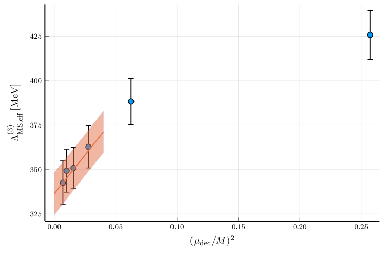
Figure 3: Values for $\Lambda^{(3)}_{\overline{\rm MS},\rm eff}$ from table 3 ($c=0.36$) and their extrapolation $M\to\infty$ using eq. (4.69) with $\hat{\Gamma}_{m}=0$.

We now proceed to investigate the effect of the logarithmic corrections. Fits with $\hat{\Gamma}_{m}=1$ yield only about 3 MeV higher values for $\Lambda$ when the $z=4$ data is excluded. Further excluding also $z=6$ reduces these shifts to only 1-2 MeV. We take the result with $z\geq 6$ and $c=0.36$ as our final result, and add 3 MeV as our estimate of the systematic effect due to the logarithmic corrections or higher orders in $1/M$ in the $M\to\infty$ extrapolation, see figure 3.

Taking all these points into account, we quote as our final result

$$\Lambda^{(3)}_{\overline{\rm MS}}=336(10)(6)_{b_{\mathrm{g}}}(3)_{\Gamma_{m}}\,{\rm MeV}=336(12)\,{\rm MeV}\,.$$ (4.70)

Here the first error is statistical, the second is due to $b_{\rm g}$ and the third results from the estimated uncertainty in the $z$-extrapolation. The combined error covers all central results that we obtained by varying the cuts in $z$, $(aM)^{2}$, and the different $\hat{\Gamma}_{m}$ except for two cases. These extreme cases have small $c\leq 0.33$ and include $z=4$ data, where corrections to decoupling are expected to be the largest. They yield Q-values below 2%.

We further note that there is a significant correlation of the above statistical error with the one of the previous work [5],

$$\Lambda^{(3)}_{\overline{\rm MS}}=341(12)\,\mathrm{MeV}\,\,,$$ (4.71)

using step scaling in the three-flavor theory up to high energy. The common piece is exactly the scale $\mu_{\mathrm{dec}}=789(15)\,\mathrm{MeV}$. The off-diagonal element of the covariance matrix of the two determinations is

$$\mathrm{Cov}(\eqref{eq:finla_lam},\eqref{eq:alpha_lam})=41\,\mathrm{MeV}^{2}\,,$$ (4.72)

compared to the diagonal ones of $144\,\mathrm{MeV}^{2}$, which at present happen to be about the same for each of the individual determinations. As a quantitative measurement of the compatibility of the two different determinations we note that their difference is not significant at all: $\Lambda\eqref{eq:alpha_lam}-\Lambda\eqref{eq:finla_lam}=5(14)\,{\rm MeV}$.

5 Result for $\alpha_{s}(m_{Z})$

Our result for $\Lambda^{(3)}_{\overline{\rm MS}}$ (eq. (4.70)) can be translated, after running across the charm and bottom quark thresholds, into a value of the four and five flavor $\Lambda$-parameter. Using the FLAG values [4] (based on [70, 71, 72, 73]) $m_{\rm c,\star}=1275(5)$ MeV, $m_{\rm b,\star}=4171(20)$ MeV for the charm and bottom quark mass thresholds, we obtain the following values for the four and five flavor $\Lambda$-parameters

$$\Lambda^{(4)}_{\overline{\rm MS}} = 294(10)(6)_{b_{\rm g}}(3)_{\Gamma_{m}}(0.7)_{3\to 4,{\rm PT}}(1)_{3\to 4,{\rm NP}}\,{\rm MeV}=294(12)\,{\rm MeV}\,,$$ (5.73)

$$\Lambda^{(5)}_{\overline{\rm MS}} = 211.3(8.1)(5.0)_{b_{\rm g}}(2.4)_{\Gamma_{m}}(0.7)_{3\to 5,{\rm PT}}(0.8)_{3\to 5,{\rm NP}}\,{\rm MeV}=211.3(9.8)\,{\rm MeV}\,.$$ (5.74)

where the first error is statistical, and the second represents the uncertainty associated with the logarithmic corrections in the limit $M\to\infty$ (see Section 4.5). The last two errors come instead from crossing the charm and bottom thresholds: first a perturbative error (determined by taking the difference in the decoupling relations and RG functions between the last two known orders), and second an estimate of 0.3% in $\Lambda^{(3)}_{\overline{\rm MS}}$ for the non-perturbative corrections in the decoupling of the charm [28].

Using the experimental value $m_{Z}=91187.6(2.1)$ MeV for the $Z$ boson pole mass [7] we get

$$\alpha_{s}(m_{Z})=0.11823(69)(42)_{b_{\rm g}}(20)_{\Gamma_{\rm m}}(6)_{3\to 5,{\rm PT}}(7)_{3\to 5,{\rm NP}}=0.11823(84)\,.$$ (5.75)

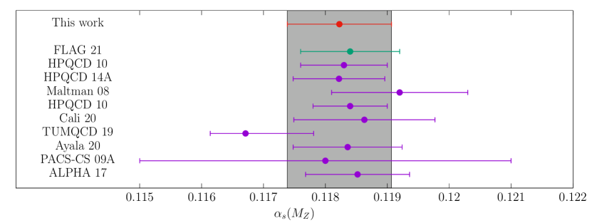
Figure 4: Our result compared with other lattice computations [18, 70, 74, 5, 75, 76, 77] that enter in the FLAG average [4] (acronyms taken from the FLAG report [4]).

Figure 4 shows a comparison of our results with other lattice computations [78, 18, 70, 74, 5, 75, 76, 77] that enter the FLAG average [4]. Our result shows a good agreement with the FLAG average, our previous determination of the strong coupling [5], and the other lattice works that enter in the FLAG average. It is important to point out that the result of this work is largely independent from our previous determination [5]. Only the value of $\mu_{\rm dec}=789(15)$ MeV is shared between both determinations of the strong coupling (see Section 4.5.2). This amounts to 28% of the squared error.

6 Conclusions and outlook

The determination of the strong coupling on the lattice faces particular challenges compared with low energy hadronic quantities. One has to connect a low energy scale with the perturbative high energy regime of QCD. Due to the slow running of the coupling, perturbative scales are very large and these two regimes cannot be comfortably simulated on a single lattice. This “window problem” which is due to the fact that only a limited range of scales can be simulated on a single lattice is the reason why most lattice determinations of the strong coupling have uncertainties dominated by the truncation errors of the perturbative series: they apply perturbation theory at in-between energy scales (see [9] for a review). One exception is the step scaling method [13], which was designed to cover a large scale difference non-perturbatively. In practice, however, the method is quite demanding, and a reduction of the current uncertainty in the strong coupling using this technique is possible but requires large computational resources.

An alternative strategy based on the decoupling of heavy quarks built on [28, 79] was formulated in ref. [1]. In short, one connects the theory with physical quark masses to the one where up, down and strange quark have masses far above the low energy QCD scales. Decoupling of the heavy quarks relates the theory to the pure gauge theory and we can use the knowledge of a pure gauge intermediate energy scale, $\mu_{\mathrm{dec}}\approx 800\leavevmode\nobreak\ {\rm MeV}$, in units of the $\Lambda_{\rm\overline{MS\kern-0.35002pt}\kern 0.35002pt}^{(0)}$ parameter. Thus the non-perturbative running between $\mu_{\mathrm{dec}}$ and perturbative scales is taken from the pure gauge theory where it is much more tractable from the numerical point of view. The connection of $\mu_{\mathrm{dec}}\approx 800\leavevmode\nobreak\ {\rm MeV}$ to the physical scales $f_{\pi}$, $f_{\rm K}$ requires only one or two step-scaling steps with light quarks; we could here take it from previous work [5].

In this paper we have worked out practical and theoretical aspects in detail and in particular demonstrated how systematic effects of various kinds can be controlled by numerical extrapolations and/or explicit computations. This is far from trivial, since a very good precision is required in all steps to reach the desired accuracy of the strong coupling. For practical reasons intermediate scales of the theory are always defined by values of associated renormalized couplings and those are defined in the Schrödinger functional. We then need to control corrections to the continuum limit and the decoupling limit of order $a$ and $1/M$ besides the ones of order $a^{2}$ and $1/M^{2}$ present also when space-time has no boundaries. We showed how the decoupling effective theory can be used to remove the $1/M$ corrections, again by non-perturbative information in the pure gauge theory, and how Symanzik and decoupling effective theories, applied in that order, restrict the form of a combined continuum and $1/M^{2}$ extrapolation of the couplings in the massive theory. Together with the high accuracy [28] of perturbation theory [34, 80, 81, 82, 83, 84] in the relation $P=\Lambda_{\rm\overline{MS\kern-0.35002pt}\kern 0.35002pt}^{(N_{\mathrm{f}})}/\Lambda_{\rm\overline{MS\kern-0.35002pt}\kern 0.35002pt}^{({N_{\mathrm{l}}})}$, which we use for $N_{\mathrm{f}}=3,{N_{\mathrm{l}}}=0$, this is a key to the precision reached in the result.

Building on these important theoretical steps, we have shown that precise results can be obtained using the decoupling strategy: our result, $\alpha_{s}(M_{Z})=0.11823(84)$, is among the most precise determinations existing so far. The error is still statistically dominated, with negligible perturbative uncertainties. This also opens the way to further reduce the current uncertainty in the strong coupling with moderate additional effort. The main sources of uncertainty are first the single step-scaling step in QCD, second the missing knowledge of the improvement parameter $b_{\rm g}$, a parameter that affects the continuum extrapolations of our massive couplings, and third the pure gauge theory non-perturbative running at high energies. The first and third source of uncertainty are statistical in nature and can be substantially improved at a modest cost with existing techniques. Lastly, a non-perturbative determination of $b_{\rm g}$ would completely eliminate the second largest source of uncertainty on our result.

Finally it is worth mentioning that the good agreement between the result of this work, and the previous determination by the ALPHA collaboration [5] (using the step-scaling method in three flavor QCD), represents a highly non-trivial cross-check of the methods.

We expect that the use of heavy quarks as a tool for non-perturbative renormalization will have more applications in the future. For example, the determination of the strong coupling directly in large volume is possible, in principle [1]. The idea can straightforwardly be applied to the determination of quark masses. Other renormalization problems, such as the determination of RGI 4-fermion operators may be tractable, but there remains work to be done in continuum perturbation theory: the high accuracy available for the perturbative decoupling of the QCD parameters  [34, 80, 81, 82, 83, 84] needs to be extended also to such operators.

Appendix A Boundary O($1/m$) contributions

A.1 Perturbative determination of $\omega_{{\rm b}}$ at leading order

In Sect. 3.3, we anticipated how relations analogous to eq. (3.53) may be used as matching conditions to determine the coefficient $\omega_{{\rm b}}$ appearing in the effective action, eq. (3.49). As also mentioned there, a convenient quantity to consider for this application is the Schrödinger functional coupling, $\bar{g}^{2}_{\rm SF}(\mu)$ [38, 14, 60]. We refer the reader to these references for a detailed definition of this coupling. For the present discussion, we recall that $\bar{g}^{2}_{\rm SF}(\mu)$ is related, up to a normalization constant $k$, to the expectation value of the $\eta$-derivative of the action, where the parameter $\eta$ enters the definition of the spatially constant Abelian boundary fields defining the SF. In formulas (cf. ref. [60]),

$${k\over\bar{g}^{2}_{\rm SF}(\mu,\bar{z})}=\langle S^{\prime}\rangle\,,\qquad S^{\prime}={{\rm d}S\over{\rm d}\eta}\,,\qquad\bar{z}=\overline{m}(\mu)/\mu\,,\qquad\mu=L^{-1}\,,$$ (A.76)

where $L$ is the spatial extent of the finite volume, and $\langle\cdot\rangle$ indicates the expectation value in QCD with $N_{\mathrm{f}}$ flavours of quarks with (renormalized) mass $\overline{m}(\mu)$ and given SF boundary conditions. A specific choice of scheme for the quark masses is not necessary for the following discussion.

Given these definitions, in the large quark mass limit, an analogous relation to eq. (3.53) holds for $S^{\prime}$, as there are no O($1/m$) corrections besides those coming from the effective action. More precisely,

$$\langle S^{\prime}\rangle=\langle S^{\prime}\rangle_{\rm dec}-\frac{1}{m_{\star}L}\omega_{{\rm b}}(\alpha_{\star})L\langle S^{\prime}S_{\rm 1,dec}\rangle_{\rm dec}+{\rm O}((m_{\star}L)^{-2})\,,$$ (A.77)

where we indicated with $\langle\cdot\rangle_{\rm dec}$ the (connected) SF correlation functions in the effective, pure Yang-Mills theory. In order to determine the lowest order coefficient in the expansion

$$\omega_{{\rm b}}(\alpha_{\star})=\omega_{\rm b}^{(1)}\,\alpha_{\star}+\omega_{\rm b}^{(2)}\,\alpha_{\star}^{2}+{\rm O}(\alpha_{\star}^{3})\,,\qquad\alpha_{\star}\equiv g^{2}_{\star}/(4\pi)=\alpha^{(N_{\mathrm{f}})}_{\overline{\rm MS}}(m_{\star})\,,$$ (A.78)

we first need the lowest order perturbative results

$$\langle S^{\prime}\rangle_{\rm dec} ={k\over[\bar{g}^{(0)}_{\rm\overline{MS\kern-0.35002pt}\kern 0.35002pt}(\mu)]^{2}}\bigg{[}1+y_{1}\,[\bar{g}^{(0)}_{\rm\overline{MS\kern-0.35002pt}\kern 0.35002pt}(\mu)]^{2}+{\rm O}([\bar{g}^{(0)}_{\rm\overline{MS\kern-0.35002pt}\kern 0.35002pt}]^{4})\bigg{]}\,,$$ (A.79)

$$-L\langle S^{\prime}S_{\rm 1,dec}\rangle_{\rm dec} ={2k\over[\bar{g}^{(0)}_{\rm\overline{MS\kern-0.35002pt}\kern 0.35002pt}(\mu)]^{2}}\bigg{[}1+c_{1}[\bar{g}^{(0)}_{\rm\overline{MS\kern-0.35002pt}\kern 0.35002pt}(\mu)]^{2}+{\rm O}([\bar{g}^{(0)}_{\rm\overline{MS\kern-0.35002pt}\kern 0.35002pt}]^{4})\bigg{]}\,,$$ (A.80)

where $\bar{g}^{(0)}_{\rm\overline{MS\kern-0.35002pt}\kern 0.35002pt}(\mu=1/L)$ is the coupling of the pure gauge theory in the $\overline{\rm MS}$-scheme. These results can be easily inferred from the pure Yang-Mills computations of refs. [85, 86]. The constants $y_{1}$ and $c_{1}$ are determined through a next-to-leading order calculation, but their actual value is not relevant at the order we are interested in. Secondly, we need the expansion

$$\langle S^{\prime}\rangle={k\over[\bar{g}^{(N_{\mathrm{f}})}_{\rm\overline{MS\kern-0.35002pt}\kern 0.35002pt}(\mu)]^{2}}\bigg{[}1+f_{1}(\bar{z})[\bar{g}^{(N_{\mathrm{f}})}_{\rm\overline{MS\kern-0.35002pt}\kern 0.35002pt}(\mu)]^{2}+{\rm O}([\bar{g}^{(N_{\mathrm{f}})}_{\rm\overline{MS\kern-0.35002pt}\kern 0.35002pt}]^{4})\bigg{]}\,,$$ (A.81)

in QCD with $N_{\mathrm{f}}$ quark flavours. In particular, we are interested in the limit of large quark masses, $\bar{z}\to\infty$, for which (cf. ref. [60]),

$$f_{1}(\bar{z})=y_{1}-\frac{1}{12\pi^{2}}N_{\mathrm{f}}\log(\bar{z})+f_{11}\frac{1}{\bar{z}}+{\rm O}(\bar{z}^{-2})\,,$$ (A.82)

where $y_{1}$ is the pure Yang-Mills result introduced earlier. As we shall see shortly, the matching coefficient $\omega_{\rm b}^{(1)}$ only depends on $f_{11}$, while the first two terms in the above equation are reabsorbed into the relation between the ${\rm\overline{MS\kern-0.50003pt}\kern 0.50003pt}$-couplings of the fundamental and effective theory. The two couplings need in fact to be matched. At the order in the perturbative expansion we are interested in, we may consider the relation (see e.g. ref. [33]),

$${1\over[\bar{g}^{(0)}_{\overline{\rm MS}}({\mu})]^{2}}={1\over[\bar{g}^{(N_{\mathrm{f}})}_{\overline{\rm MS}}({\mu})]^{2}}\bigg{[}1+h_{1}({\bar{z}})[\bar{g}^{(N_{\mathrm{f}})}_{\overline{\rm MS}}({\mu})]^{2}+{\rm O}([\bar{g}^{(N_{\mathrm{f}})}_{\overline{\rm MS}}]^{4})\bigg{]}\,,\quad h_{1}({\bar{z}})=-{1\over 12\pi^{2}}N_{\mathrm{f}}\log(\bar{z})\,.$$ (A.83)

We can now combine the results of eqs. (A.77)-(A.83). Noticing that: $[\bar{g}^{(0)}_{\overline{\rm MS}}(\mu))]^{2}=[\bar{g}^{(N_{\mathrm{f}})}_{\overline{\rm MS}}(\mu)]^{2}+{\rm O}([\bar{g}^{(N_{\mathrm{f}})}_{\overline{\rm MS}}]^{4})=g_{\star}^{2}+{\rm O}(g_{\star}^{4})$ and $\overline{m}(\mu)=m_{\star}(1+{\rm O}(g_{\star}^{2}))$, neglecting higher-order terms in $1/\bar{z}$ and $g_{\star}^{2}$, we arrive at the sought after relation

$$\omega_{\rm b}^{(1)}=2\pi f_{11}\,.$$ (A.84)

The value of $f_{11}$ can be inferred from the 1-loop calculation of the massive SF coupling of ref. [60]. More precisely, eqs. (3.17)-(3.18) of this reference give $f_{11}=q_{1}/(4\pi)$. For definiteness, we take the result $q_{1}=-0.10822$, obtained for $\theta=\pi/5$, as this coupling definition shows significantly smaller O($1/\bar{z}^{2}$) corrections than the definition with $\theta=0$. We can in fact use the difference between the results for $\theta=0,\pi/5$ as an estimate of the systematic uncertainties involved in the extraction of $q_{1}$. In conclusion, we find:

$$\omega_{{\rm b}}^{(1)}=-0.0541(5)N_{\rm f}\,.$$ (A.85)

A.2 Estimates of the O($1/m$) boundary effects

A.2.1 Definitions

Given $\omega_{{\rm b}}$ at leading order in perturbation theory, we can now employ eq. (3.53) to get an estimate of the O($1/M$) corrections to the massive GFT-coupling $\bar{g}^{(3)}_{\rm GFT,c}(\mu_{\rm dec},M)$, defined in the SF with temporal extent $T=2L$, and evaluated at the renormalization scale $\mu_{\rm dec}=1/L_{\rm dec}$. (As usual, $M$ is the RGI mass of the degenerate heavy quarks in the $N_{\mathrm{f}}=3$ theory and $c=\sqrt{8t}/L$, with $t$ the flow time at which the coupling is measured.) To this end, we define,

$$\Delta_{\rm c}(z)\equiv[\bar{g}^{(3)}_{\rm GFT,c}(\mu_{\rm dec},M)]^{2}-[\bar{g}^{(0)}_{\rm GFT,c}(\mu_{\rm dec})]^{2}\,,\qquad z=M/\mu_{\rm dec}\,,$$ (A.86)

where we implicitly assume that the $\Lambda$-parameters in the two theories have been properly matched. Applying eq. (3.53) to the case at hand we have,

$$\Delta_{\rm c}(z)\overset{z\to\infty}{\approx}-{\omega_{{\rm b}}(\alpha_{\star})\over z}\bigg{(}{M\over m_{\star}}\bigg{)}\lim_{a\to 0}\,L_{\rm dec}\,\mathcal{N}^{-1}{\langle t^{2}E_{\rm mag}(t,T/2)\hat{\delta}(Q)S_{\rm 1,dec}^{R}\rangle_{\rm dec}\over\langle\hat{\delta}(Q)\rangle_{\rm dec}}+{\rm O}\big{(}{z^{-2}}\big{)}\,,$$ (A.87)

where, we recall, $\alpha_{\star}\equiv g^{2}_{\star}/(4\pi)$ with $g_{\star}\equiv\bar{g}_{\overline{\rm MS}}(m_{\star})$ and $m_{\star}=\overline{m}_{\overline{\rm MS}}(m_{\star})$, and we take the connected part of the (ratio of) correlation functions. In the above equation we use the short hand notation (cf. eq. (2.13))

$$[\bar{g}^{(0)}_{\rm GFT,c}(\mu)]^{2}=\mathcal{N}^{-1}{\langle t^{2}E_{\rm mag}(t,T/2)\hat{\delta}(Q)\rangle_{\rm dec}\over\langle\hat{\delta}(Q)\rangle_{\rm dec}}\,,\quad\mu=1/L\,,\quad T=2L\,,\quad c=\sqrt{8t}/L\,,$$ (A.88)

for the definition of the ${\rm GFT}$-coupling in the pure-gauge theory. The field $E_{\rm mag}(t,x_{0})$ represents our chosen discretization for the magnetic component of the energy density at positive flow time. For the latter, we consider the Zeuthen flow for the discretization of the flow equations [52], while for the observable we take the specific combination of plaquette and clover discretizations of the flow energy density proposed in ref. [52], which is O($a^{2}$)-improved. The quantity $\hat{\delta}(Q)$ is instead a discretization of the continuum $\delta$-function that projects to the topological $Q=0$ sector. It is zero whenever $|Q|>0.5$ and one otherwise, with $Q$ the topological charge computed with the clover discretization of the field strength tensor built from gauge fields flowed at time $\sqrt{8t}=cL$ using the Zeuthen flow (cf. e.g. ref. [35]). In order to evaluate the correlation function in eq. (A.87) on the lattice, we also need a viable discretization for $S_{\rm 1,dec}$. We choose,

$$S^{R}_{\rm 1,dec}=a^{3}\sum_{\mathbf{x}}\,\big{[}\mathcal{O}^{R}_{{\rm b}}(0,\bm{x})+\mathcal{O}^{R}_{{\rm b}}(T-a,\bm{x})\big{]}\,,\quad\mathcal{O}^{R}_{\rm b}(x_{0},\bm{x})=Z_{\rm b}(g_{0})\mathcal{O}_{\rm b}(x_{0},\bm{x})\,,$$ (A.89)

where

$$a^{4}\mathcal{O}_{\rm b}(x_{0},\bm{x})={2\over g_{0}^{2}}\sum_{k=1}^{3}{\rm Re}\,{\rm tr}\big{[}1-U_{0k}(x_{0},\bm{x})\big{]}\,,\quad x_{0}=0,T-a\,,$$ (A.90)

with $U_{\mu\nu}(x)$ being the plaquette at $x$ in the $\mu,\nu$-direction. As discussed in Sect. 3.3, on the lattice, the boundary field $\mathcal{O}_{\rm b}$ requires a finite renormalization. In the following, we consider the 1-loop approximation [87]

$$Z_{\rm b}(g_{0})=1-0.13194\,g_{0}^{2}+{\rm O}(g_{0}^{4})\,,$$ (A.91)

which can be readily inferred from the renormalization of the energy density in the pure-gauge theory obtained in this reference.

In practice, we can evaluate the correlator in eq. (A.87) by exploiting the identity (note the appearance of the bare boundary action)

$$-L\,\mathcal{N}^{-1}{\langle t^{2}E_{\rm mag}(t,T/2)\hat{\delta}(Q)S_{\rm 1,dec}\rangle_{\rm dec}\over\langle\hat{\delta}(Q)\rangle_{\rm dec}}\,={L\over a}{{\rm d}[\bar{g}_{\rm GFT,c}^{(0)}(\mu)]^{2}\over{\rm d}c_{\rm t}}\,.$$ (A.92)

Thus, the connected correlator of interest can be computed by varying the boundary O($a$) improvement coefficient $c_{\rm t}$ in simulations (cf. Appendix C). Given the result in eq. (A.87), and defining

$$p_{\rm c}(\bar{g})\equiv\bigg{[}\lim_{a\to 0}Z_{\rm b}(g_{0}){L\over a}{{\rm d}[\bar{g}_{\rm GFT,c}^{(0)}(\mu)]^{2}\over{\rm d}c_{\rm t}}\bigg{]}\bigg{|}_{\bar{g}}\,,$$ (A.93)

we have that the leading-order (LO) estimate for the relative O($1/M$) corrections to the GFT-coupling can be written as,

$${\Delta_{\rm c}(z)\over\bar{g}^{2}_{\rm c}(z)}\Bigg{|}_{\rm LO}={1\over(4\pi)}{\omega_{\rm b}^{(1)}\over z}\bigg{(}{M\over m_{\star}}\bigg{)}\Bigg{(}{g_{\star}^{2}\over\bar{g}^{2}_{\rm c}(z)}\Bigg{)}p_{\rm c}(\bar{g}^{2}_{\rm c}(z))+{\rm O}\bigg{(}g_{\star}^{2},{1\over z^{2}}\bigg{)}\,,$$ (A.94)

where we introduced the shorthand notation: $\bar{g}_{\rm c}(z)\equiv\bar{g}^{(3)}_{\rm GFT,c}(\mu_{\rm dec},M)$.

A.2.2 Simulation results

$c$	$L/a$	$\beta$	$[\bar{g}^{(0)}_{\rm GFT,c}]^{2}$	$\frac{L}{a}\frac{{\rm d}[\bar{g}^{(0)}_{\rm GFT,c}]^{2}}{{\rm d}c_{\rm t}}$
$0.3$	$10$	$6.2556$	$4.8513(22)$	$-0.46(14)$
	$10$	$6.3400$	$4.4462(19)$	$-0.45(12)$
	$10$	$6.4200$	$4.1359(17)$	$-0.43(11)$
$0.3$	$12$	$6.4200$	$4.6805(20)$	$-0.45(15)$
	$12$	$6.4630$	$4.4895(19)$	$-0.54(15)$
	$12$	$6.5619$	$4.1094(17)$	$-0.28(13)$
$0.3$	$16$	$6.6669$	$4.7627(14)$	$-0.42(09)$
	$16$	$6.6920$	$4.6515(19)$	$-0.55(12)$
	$16$	$6.7140$	$4.5641(19)$	$-0.52(12)$
	$16$	$6.7859$	$4.2942(12)$	$-0.25(08)$
$0.42$	$10$	$6.2556$	$7.5116(61)$	$-2.91(38)$
	$10$	$6.3400$	$6.6790(52)$	$-2.35(32)$
	$10$	$6.4200$	$6.0807(44)$	$-1.98(28)$
$0.42$	$12$	$6.4200$	$7.1857(57)$	$-2.36(43)$
	$12$	$6.4630$	$6.7975(52)$	$-2.42(40)$
	$12$	$6.5619$	$6.0584(44)$	$-1.68(34)$
$0.42$	$16$	$6.6669$	$7.1159(39)$	$-2.21(25)$
	$16$	$6.6920$	$6.8934(51)$	$-2.29(33)$
	$16$	$6.7140$	$6.7275(50)$	$-2.19(32)$
	$16$	$6.7859$	$6.2173(32)$	$-1.52(21)$

Table 5: Results for the $\Delta c_{\rm t}\to 0$ extrapolations, eq. (A.95), for different values of $L/a$, $c$, and couplings $[\bar{g}^{(0)}_{\rm GFT,c}]^{2}$. The results refer to the magnetic coupling discretized using the Zeuthen flow and O($a^{2}$)-improved plaquette + clover definition of the flow energy density [52]. We considered linear extrapolations in $(\Delta c_{\rm t})^{2}$ using all available $\Delta c_{\rm t}$ values.

In order to estimate the relevant $c_{\rm t}$-derivatives in eq. (A.92), we simulated lattices with $L/a=10,12,16$ using the Wilson-plaquette gauge action, and varied $c_{\rm t}$ around its two-loop value $c_{\rm t}^{\star}$ [86], i.e. $c_{\rm t}^{\pm}=c_{\rm t}^{\star}\pm\Delta c_{\rm t}$. For $L/a=10,12$, we considered variations $\Delta c_{\rm t}=\{0.075,0.1,0.15,0.2\}$, while for $L/a=16$ we took $\Delta c_{\rm t}=\{0.1,0.15,0.2,0.3\}$. For $L/a=10,12$ and $L/a=16$ we simulated 3 and 4 values of $\beta$, respectively, in order to cover the relevant range of values for $[\bar{g}^{(0)}_{\rm GFT,c}]^{2}$; this for two schemes $c=0.3,0.42$. In Table 5 we collect the results for

$${L\over a}{{\rm d}[\bar{g}_{\rm GFT,c}^{(0)}(\mu)]^{2}\over{\rm d}c_{\rm t}}=\lim_{\Delta c_{\rm t}\to 0}{L\over a}{\Delta[\bar{g}^{(0)}_{\rm GFT,c}]^{2}\over 2\Delta c_{\rm t}},\quad\Delta[\bar{g}^{(0)}_{\rm GFT,c}]^{2}\equiv[\bar{g}^{(0)}_{\rm GFT,c}(\mu)]^{2}|_{c_{\rm t}^{+}}-[\bar{g}^{(0)}_{\rm GFT,c}(\mu)]^{2}|_{c_{\rm t}^{-}}\,,$$ (A.95)

obtained as linear extrapolations in $(\Delta c_{\rm t})^{2}$ using all available $\Delta c_{\rm t}$. The sum, $\chi^{2}_{\rm tot}$, of the $\chi^{2}$’s of all fits is good, i.e. $\chi_{\rm tot}^{2}/{\rm d.o.f.}_{\rm tot}\approx 1$, with ${\rm d.o.f.}_{\rm tot}$ the total number of degrees of freedom considering all fits. At the level of individual fits, these have a $\chi^{2}$ up to $\approx 7$ for two degrees of freedom.

In Table 7 we report the results for the $c_{\rm t}$-derivatives of the $N_{\mathrm{f}}=0$ coupling interpolated at the values of the coupling of interest. The latter are specified by the results in the $N_{\mathrm{f}}=3$-theory (cf. Table 2):

$$\bar{g}^{2}_{\rm 0.30}(z=6)=4.490(50)\,,\qquad\bar{g}^{2}_{\rm 0.42}(z=4)=6.68(10)\,.$$ (A.96)

For the interpolations we considered the following functional form,

$${L\over a}{{\rm d}[\bar{g}^{(0)}_{\rm GFT,c}]^{2}\over{\rm d}c_{\rm t}}=\sum_{k=1}^{3}c_{k}\,[\bar{g}^{(0)}_{\rm GFT,c}]^{2k}\,,$$ (A.97)

where the value of $c_{1}$ is fixed to its tree-level result (cf. Table 6).

$c$	$L/a$	${1\over g_{0}^{2}}\frac{L}{a}\frac{{\rm d}[\bar{g}^{(0)}_{\rm GFT,c}]^{2}}{{\rm d}c_{\rm t}}\times 10^{4}$
$0.3$	$10$	$-2.6042383805$
	$12$	$-2.4106092056$
	$16$	$-2.2186159754$
$0.42$	$10$	$-12.918755710$
	$12$	$-12.000133367$
	$16$	$-11.123348145$

Table 6: Results for the $c_{\rm t}$-derivative of the GFT-coupling at tree-level in lattice perturbation theory. The results refer to the magnetic coupling discretized using the Zeuthen flow and O($a^{2}$)-improved plaquette + clover definition of the flow energy density [52].

Once the results for the different $L/a$ were interpolated to a fixed value of the coupling and properly renormalized with the 1-loop value of $Z_{\rm b}$, eq. (A.91), we performed an extrapolation to $a/L\to 0$, assuming leading O($a$) effects. The results are reported in Table 8, while Figure 5 illustrates the corresponding extrapolations. The results for $p_{\rm c}(\bar{g})$ for $c=0.42$ tend to be larger (in module) than those for $c=0.30$. This is expected, as the footprint of the flow energy density defining the GFT-coupling extends closer to the SF boundaries for $c=0.42$, therefore increasing the sensitivity to the ${\rm O}(1/M)$ counterterms.

$c$	$L/a$	$\beta$	$[\bar{g}^{(0)}_{\rm GFT,c}]^{2}$	$\frac{L}{a}\frac{{\rm d}[\bar{g}^{(0)}_{\rm GFT,c}]^{2}}{{\rm d}c_{\rm t}}$
$0.3$	$10$	$6.3299(4)$	$4.490$	$-0.45(7)$
	$12$	$6.4629(5)$	$4.490$	$-0.44(9)$
	$16$	$6.7324(4)$	$4.490$	$-0.37(5)$
$0.42$	$10$	$6.3399(6)$	$6.68$	$-2.35(19)$
	$12$	$6.4771(7)$	$6.68$	$-2.14(23)$
	$16$	$6.7196(6)$	$6.68$	$-1.94(13)$

Table 7: Results of the interpolations eq. (A.97) using the values in Table 5 and the target couplings, eq. (A.96). (Note that we did not propagate the error on $[\bar{g}^{(0)}_{\rm GFT,c}]^{2}$ to the $c_{\rm t}$-derivatives.) All fits have good or acceptable $\chi^{2}$. The values of $\beta$ have been obtained by a quadratic interpolation of the results for $[\bar{g}^{(0)}_{\rm GFT,c}]^{-2}$ from Table 5 as a function of $g_{0}^{-2}$.

$c$	$[\bar{g}^{(0)}_{\rm GFT,c}]^{2}$	$L/a$	$p_{\rm c}$
$0.3$	$4.490$	$10$	$-0.39(6)$
		$12$	$-0.39(8)$
		$16$	$-0.33(4)$
		$\infty$	$-0.21(16)$
$0.42$	$6.68$	$10$	$-2.06(17)$
		$12$	$-1.88(20)$
		$16$	$-1.71(11)$
		$\infty$	$-1.14(41)$

Table 8: Results for $p_{\rm c}$ at finite lattice spacing (cf. eq. (A.93)) obtained using the values for the $c_{\rm t}$-derivatives of the GFT-coupling in Table 7 and the 1-loop approximation for $Z_{\rm b}$, eq. (A.91). The results of a $L/a\to\infty$ extrapolation linear in $a/L$ are also given.

Figure 5: Illustrative continuum limit extrapolations for the $p_{\rm c}$ results of Table 8.

A.2.3 O($1/M$) corrections: LO estimates

We first estimate $\Delta_{\rm c}(z)$ corresponding to the coupling at $z=6$ and $c=0.3$ (cf. eq. (A.96)). In this case we have,

$$\bar{g}^{2}_{0.3}(z=6)=4.490(50)\,,\qquad g^{2}_{\star}\approx 3\,,\qquad M/m_{\star}\approx 1.5\,,$$ (A.98)

where to compute $g_{\star}$ we used

$${M\over\Lambda^{(N_{\mathrm{f}}=3)}_{\overline{\rm MS}}}=z\times{\mu_{\rm dec}\over\Lambda^{(N_{\mathrm{f}}=3)}_{\overline{\rm MS}}}\,,$$ (A.99)

with $\mu_{\rm dec}=789\,{\rm MeV}$ and $\Lambda^{(N_{\mathrm{f}}=3)}_{\overline{\rm MS}}=341\,{\rm MeV}$. For the ${\rm O}(1/M)$ counterterm $p_{\rm c}$ we take the result (cf. Table 8),

$$p_{0.30}(\bar{g}^{2}_{0.30}(z=6))=-0.21\,.$$ (A.100)

Putting the numbers together we obtain for the LO estimate, eq. (A.94),

$${\Delta_{0.3}(z=6)\over\bar{g}^{2}_{0.30}(z=6)}\Bigg{|}_{\rm LO}\approx 5\times 10^{-4}\,.$$ (A.101)

This is about a factor 20 smaller than the statistical error on the coupling.

As a second case, we estimate $\Delta_{\rm c}(z)$ for $z=4$ and $c=0.42$. In this case we have,

$$\bar{g}^{2}_{0.42}(z=4)=6.68(10)\,,\qquad g^{2}_{\star}\approx 3.5\,,\qquad M/m_{\star}\approx 1.4\,.$$ (A.102)

For the O($1/M$) counterterm $p_{\rm c}$ we take the result (cf. Table 8)

$$p_{0.42}(\bar{g}^{2}_{0.42}(z=4))=-1.14\,.$$ (A.103)

Putting the numbers together we obtain for the LO estimate, eq. (A.94),

$${\Delta_{\rm 0.42}(z=4)\over\bar{g}^{2}_{0.42}(z=4)}\Bigg{|}_{\rm LO}\approx 3\times 10^{-3}\,,$$ (A.104)

which is about a factor 5-6 smaller than the statistical error on the coupling. A slightly more conservative estimate may be obtained in this case by taking $p_{0.42}=-1.71$, which corresponds to the result at the smallest lattice spacing we simulated, i.e. $L/a=16$. In this case, the systematic O($1/M$) effects are about 3-4 times smaller than the statistical error on the coupling. The smallest value of $z$ entering the analysis of Sect. 4.5.2 is $z=6$. Considering that these effects decrease linearly with increasing $z$ and that the results for $c=0.42$ offer an upper-bound for values of $c<0.42$, it appears to be safe to assume that ${\rm O}(1/M)$ effects can be neglected altogether.

Appendix B Summary of pure-gauge results

B.1 Matching GF and GFT schemes at the decoupling scale

As explained in Sect. 2.1, we need the continuum relation

$$\bar{g}^{(0)}_{\rm GF}(\mu)=\chi_{\rm c}\left(\bar{g}^{(0)}_{\rm GFT,c}(\mu)\right)$$ (B.105)

for $\mu$ around $\mu_{\mathrm{dec}}$, i.e. $\bar{g}^{(0)}_{\rm GFT,c}=\bar{g}^{(3)}_{\rm GFT,c}(\mu_{\rm dec},M)$ is in the range of Tables 2 and 3. On a finite lattice, eq. (B.105) is obtained by computing both couplings at the same $L/a=1/(\mu a)$ and $\beta$ and the relation contains discretization errors of order $(a/L)^{2}$. Results of our simulations for $L/a=12,\ldots,48$ and $\beta\in[6.2,7.6]$ are reported in Table 9. We parameterize the data by

$$\frac{1}{[\bar{g}^{(0)}_{\text{GFT,c}}]^{2}}-\frac{1}{[\bar{g}^{(0)}_{\text{\rm GF}}]^{2}}=P^{\rm c}_{n_{p}}([\bar{g}^{(0)}_{\text{\rm GF}}]^{2})+\Big{(}{a\over L}\Big{)}^{2}Q_{n_{q}}^{\rm c}([\bar{g}^{(0)}_{\text{\rm GF}}]^{2})\,,$$ (B.106)

where $P_{n_{p}}^{\rm c}(g^{2})$, $Q_{n_{q}}^{c}(g^{2})$ are polynomials of degree $n_{p}$ and $n_{q}$, respectively. The sought-after continuum relation (B.105) is then implicitly given in terms of

$$P^{\rm c}_{n_{p}}(g^{2})=\sum_{k=0}^{n_{p}}p^{\rm c}_{k}\,g^{2k}\,,$$ (B.107)

through,

$$[\chi_{\rm c}^{-1}(g)]^{2}=\frac{g^{2}}{1+g^{2}P^{\rm c}_{n_{p}}(g^{2})}\,,$$ (B.108)

where $\chi_{\rm c}^{-1}$ is the inverse of the function $\chi_{\rm c}$. For all values of $c=0.3-0.42$, taking $n_{p}=n_{q}=2$ already yields good fits. As an illustrative example, we give here the results for $P^{\rm c}_{2}$ for the case $c=0.3$, where we find ($p_{k}\equiv p^{0.3}_{k}$)

$$p_{0} = -1.6168053320710727\times 10^{-2}\,,$$ (B.109)

$$p_{1} = -1.6086523109487365\times 10^{-4}\,,$$ (B.110)

$$p_{2} = -3.0358986840266259\times 10^{-5}\,,$$ (B.111)

with covariance

$$\mathrm{cov}(p_{i},p_{j})=\left(\begin{array}[]{lll}2.92499121\times 10^{-4}&-1.29098204\times 10^{-4}&1.41308163\times 10^{-5}\\ -1.29098204\times 10^{-4}&5.73202489\times 10^{-5}&-6.27896098\times 10^{-6}\\ 1.41308163\times 10^{-5}&-6.27896098\times 10^{-6}&6.91910100\times 10^{-7}\\ \end{array}\right)\,.$$ (B.112)

Figure 6 demonstrates that the discretization errors are small and our largest lattice results are in agreement with the continuum band. Note that, the error of $P^{\rm c}_{2}$, computable in terms of (B.112) for the case of $c=0.3$, is negligible in the final $\Lambda^{(3)}_{\overline{\rm MS}}/\mu_{\rm dec}$ determination for all values of $c$ considered.

$L/a$	$\beta$	$[\bar{g}^{(0)}_{\text{GF}}]^{2}$	$[\bar{g}^{(0)}_{\text{GFT,0.30}}]^{2}$	$[\bar{g}^{(0)}_{\text{GFT,0.33}}]^{2}$	$[\bar{g}^{(0)}_{\text{GFT,0.36}}]^{2}$	$[\bar{g}^{(0)}_{\text{GFT,0.39}}]^{2}$	$[\bar{g}^{(0)}_{\text{GFT,0.42}}]^{2}$
12	6.2556	5.1104(49)	5.6616(89)	6.329(12)	7.141(16)	8.144(22)	9.393(30)
12	6.2643	5.0690(50)	5.5995(84)	6.251(11)	7.042(15)	8.018(20)	9.232(27)
12	6.2654	5.0489(49)	5.5876(90)	6.232(12)	7.013(16)	7.977(21)	9.175(29)
12	6.3451	4.6316(71)	5.0759(72)	5.6147(94)	6.264(12)	7.060(16)	8.043(21)
12	6.3509	4.6164(43)	5.0329(72)	5.5618(93)	6.199(12)	6.980(16)	7.942(20)
12	6.3560	4.5905(68)	5.0078(69)	5.5318(90)	6.163(12)	6.936(16)	7.889(21)
12	6.3642	4.5554(44)	4.9594(69)	5.4718(88)	6.088(11)	6.842(15)	7.771(20)
12	6.3894	4.4339(44)	4.8288(65)	5.3162(86)	5.901(11)	6.613(15)	7.490(20)
12	6.4133	4.3543(40)	4.7133(63)	5.1798(82)	5.739(10)	6.421(13)	7.258(17)
12	6.4200	4.3136(40)	4.6821(68)	5.1419(87)	5.694(11)	6.366(14)	7.192(18)
12	6.4630	4.1590(38)	4.4928(63)	4.9196(78)	5.4311(99)	6.053(13)	6.816(16)
12	6.5619	3.8287(34)	4.1143(55)	4.4749(69)	4.9051(88)	5.426(11)	6.063(14)
16	6.4200	5.3833(70)	6.0206(99)	6.781(13)	7.710(19)	8.864(26)	10.313(35)
16	6.4740	5.0535(67)	5.5929(85)	6.247(11)	7.040(15)	8.018(20)	9.233(27)
16	6.4741	5.0594(49)	5.5766(89)	6.230(12)	7.023(16)	7.999(21)	9.214(28)
16	6.5619	4.6165(56)	5.0554(71)	5.5943(94)	6.242(12)	7.034(16)	8.009(21)
16	6.6669	4.2007(56)	4.5412(61)	4.9771(78)	5.498(10)	6.131(13)	6.908(17)
16	6.7859	3.8249(45)	4.0969(56)	4.4595(76)	4.8915(97)	5.415(12)	6.054(16)
16	6.8000	3.7825(44)	4.0449(56)	4.3998(70)	4.8238(88)	5.338(11)	5.968(14)
20	6.6669	4.9431(61)	5.4190(86)	6.037(11)	6.785(15)	7.705(19)	8.846(26)
20	6.7859	4.4082(54)	4.7887(68)	5.2779(89)	5.865(11)	6.581(15)	7.462(19)
20	6.8000	4.3553(53)	4.7153(64)	5.1890(83)	5.757(11)	6.449(14)	7.299(18)
20	6.8637	4.1219(48)	4.4531(60)	4.8781(77)	5.3855(99)	6.001(13)	6.756(16)
20	6.9595	3.8245(44)	4.0977(54)	4.4637(69)	4.9001(87)	5.429(11)	6.076(14)
24	6.7859	5.0578(61)	5.5530(79)	6.206(10)	6.999(14)	7.978(19)	9.196(25)
24	6.8637	4.6776(56)	5.1006(66)	5.6520(86)	6.316(11)	7.130(15)	8.135(19)
24	6.9595	4.2884(52)	4.6378(61)	5.0988(79)	5.651(10)	6.324(13)	7.150(17)
24	7.1146	3.7942(53)	4.0599(50)	4.4194(63)	4.8479(80)	5.367(10)	6.002(13)
32	6.9595	5.345(14)	5.926(11)	6.666(14)	7.570(19)	8.694(26)	10.103(35)
32	7.1146	4.5866(93)	4.9887(70)	5.5195(91)	6.158(12)	6.937(16)	7.898(20)
32	7.2000	4.2584(90)	4.5933(63)	5.0480(82)	5.592(10)	6.255(13)	7.069(17)
48	7.6000	4.0120(74)	4.3161(61)	4.7213(79)	5.205(10)	5.792(13)	6.512(17)

Table 9: Data used for the matching of the $T=L$ and $T=2L$ schemes.

Figure 6: Fit to match the schemes $\bar{g}^{(0)}_{\text{GF}}$ and $\bar{g}^{(0)}_{\text{\rm GFT,c}}$ for $c=0.3$.

B.2 High-energy running

In this appendix we collect the main ingredients for the determination of

$$\frac{\Lambda^{(0)}_{\overline{\rm MS}}}{\mu_{\rm dec}}=\frac{\Lambda^{(0)}_{\overline{\rm MS}}}{\Lambda^{(0)}_{\rm GF}}\varphi_{\rm GF}^{(0)}(\bar{g}^{(0)}_{\text{GF}}(\mu_{\mathrm{dec}}))\,,$$ (B.113)

where we recall that it will be used with $\bar{g}^{(0)}_{\text{GF}}(\mu_{\mathrm{dec}})=\chi_{\rm c}(\bar{g}^{(3)}_{\rm GFT,c}(\mu_{\rm dec},M))$, cf. Table 2. Following [2, 3], we rewrite eq. (B.113) as

$$\frac{\Lambda^{(0)}_{\overline{\rm MS}}}{\mu_{\rm dec}}=\frac{\Lambda^{(0)}_{\overline{\rm MS}}}{\mu_{\rm swi}}\times{\mu_{\rm swi}\over{\mu_{\rm dec}}}\quad\text{where}\quad[\bar{g}^{(0)}_{\rm GF}(\mu_{\rm swi})]^{2}={4\pi\over 5}\,,$$ (B.114)

and insert [2]

$$\frac{\Lambda^{(0)}_{\overline{\rm MS}}}{\mu_{\rm swi}}=0.2658(36)\,.$$ (B.115)

With given $\bar{g}^{(0)}_{\rm GF}(\mu_{\rm dec})$, the ratio of scales ${\mu_{\rm swi}/{\mu_{\rm dec}}}$ can be obtained through the relation

$$\ln\bigg{(}{\mu_{\rm swi}\over{\mu_{\rm dec}}}\bigg{)}=\int^{\bar{g}^{(0)}_{\rm GF}(\mu_{\rm swi})}_{\bar{g}^{(0)}_{\rm GF}(\mu_{\rm dec})}{{\rm d}g\over\beta_{\rm GF}^{(0)}(g)}\,,$$ (B.116)

where $\beta_{\rm GF}^{(0)}$ is the non-perturbative $\beta$-function for $\bar{g}^{(0)}_{\rm GF}(\mu)$. In the region of couplings, $\bar{g}^{(0)}_{\rm GF}\in[2,11]$, a convenient parametrization for the needed $\beta$-function is given by

$$\beta_{\rm GF}^{(0)}(\bar{g})=-{\bar{g}^{3}\over\sum_{k=0}^{3}p_{k}\bar{g}^{2k}}\,,$$ (B.117)

with coefficients

$$p_{0}=14.93613381\,,\quad p_{1}=-1.03947429\,,\quad p_{2}=0.18007512\,,\quad p_{3}=-0.01437036\,,$$ (B.118)

and covariance

$${\rm cov}(p_{i},p_{j})=\\[4.30554pt] \left(\begin{array}[]{cccc}5.24669327\times 10^{\text{-1}}&-3.26120586\times 10^{\text{-1}}&6.03484522\times 10^{\text{-2}}&-3.33454413\times 10^{\text{-3}}\\ -3.26120586\times 10^{\text{-1}}&2.07627940\times 10^{\text{-1}}&-3.91082685\times 10^{\text{-2}}&2.19046893\times 10^{\text{-3}}\\ 6.03484522\times 10^{\text{-2}}&-3.91082685\times 10^{\text{-2}}&7.47684098\times 10^{\text{-3}}&-4.23948184\times 10^{\text{-4}}\\ -3.33454413\times 10^{\text{-3}}&2.19046893\times 10^{\text{-3}}&-4.23948184\times 10^{\text{-4}}&2.42972883\times 10^{\text{-5}}\\ \end{array}\right)\,.$$ (B.119)

In ref. [2] a similar representation of a pure gauge theory $\beta$-function is given which applies to the coupling defined by the electric components of the flow energy density instead of our choice eq. (2.11). For completeness, we collect in Table 10 the values for ${\Lambda^{(0)}_{\overline{\rm MS}}}/{\mu_{\rm dec}}$ obtained by combining the results for the massive couplings in Table 2, the matching relation, eq. (B.106), and the high-energy running, eqs. (B.115)-(B.116).

	$\Lambda_{\overline{\rm MS}}^{(0)}/\mu_{\rm dec}$
$z$	$c=0.30$	$c=0.33$	$c=0.36$	$c=0.39$	$c=0.42$
1.972	0.685(13)	0.681(13)	0.678(14)	0.677(14)	0.678(14)
4	0.723(15)	0.720(15)	0.719(16)	0.718(16)	0.719(16)
6	0.740(16)	0.736(16)	0.734(16)	0.732(16)	0.731(16)
8	0.760(18)	0.756(18)	0.753(17)	0.750(17)	0.748(17)
10	0.787(20)	0.785(20)	0.783(19)	0.781(19)	0.780(19)
12	0.802(21)	0.799(21)	0.797(21)	0.794(21)	0.793(21)

Table 10: Results for $\Lambda_{\overline{\rm MS}}^{(0)}/\mu_{\rm dec}$ corresponding to different values of $\bar{g}^{(3)}_{\rm GFT,c}(\mu_{\rm dec},M)$ of Table 2.

Appendix C Simulations

We use a variant of the open-source (GPL v2) package openQCD version 1.6 [88, 89] in plain C with MPI parallelization. This software has been successfully used in various large-scale projects. The simulations are performed on lattices of size $\frac{T}{a}\times\left(\frac{L}{a}\right)^{3}$. We impose Schrödinger Functional (SF) boundary conditions on the gauge and fermion fields [38, 39], i.e., Dirichlet boundary conditions in Euclidean time at $x_{0}=0,T$, and periodic (up to a phase $e^{i\theta}$ for fermionic fields, with $\theta=0.5$) boundary conditions with period $L$ in the three spatial directions. We use one-loop boundary improvement coefficients $c_{\rm t}$ and $\tilde{c}_{\rm t}$ [90, 35]. Our lattice setup uses non-perturbatively ${\rm O}(a)$-improved Wilson fermions and the tree-level Symanzik ${\rm O}(a^{2})$-improved gauge action [65]; we refer the reader to ref. [35] for more details. The bare (linearly divergent) quark mass is denoted by $m_{0}$ and the pure gauge action has a prefactor $\beta=6/g_{0}^{2}$. The ensemble generation proceeds according to a variant of the Hybrid Monte-Carlo (HMC) algorithm [91]. The classical equations of motion are solved numerically for trajectories of length $\tau=2$ in all simulations, leading to Metropolis proposals. In order to reduce the computational cost and obtain a high acceptance rate, we split the action and corresponding forces as follows. For the u/d quark doublet we use an even–odd preconditioned [92] Dirac operator and Hasenbusch’s mass factorization [93] with twisted masses [94] of increasing values $\mu_{0}<\mu_{1}\ldots$ roughly set at equal distances on a logarithmic scale as suggested in Ref. [95]. The strange quark is simulated with the rational hybrid Monte-Carlo (RHMC) algorithm [96, 97], decomposing the fermion determinant into a reweighting factor and a Zolotarev optimal rational approximation of $(\hat{D}^{\dagger}\hat{D})^{-1/2}$ [98] in the spectral range $[r_{a},r_{b}]$ of $\hat{D}^{\dagger}\hat{D}$ with a number of poles $N_{p}$. The algorithmic simulation parameters are summarized in table 11. The measurements (gradient flow observables, correlation functions and reweighting factors) are done during ensemble generation.

ensemble	massless	massive
Force 0, level	gauge, 0	gauge, 0
Force 1, level	TM1-EO-SDET, 1	TM1-EO-SDET, 1
Force 2, level	TM2-EO, 1	TM2-EO, 1
Force 3, level	TM2-EO, 1	TM2-EO, 2
Force 4, level	RAT-SDET, 1	TM2-EO, 1
Force 5, level	-	RAT, 2
Level 0, nstep	OMF4, 1	OMF4, 1
Level 1, nstep	OMF4, 8-10	OMF4, 1
Level 2, nstep	-	OMF2, 6
Solver 0, res	CGNE $10^{-12}$	CGNE $10^{-11}$
Solver 1, res	DFL_SAP_GCR $10^{-12}$	DFL_SAP_GCR $10^{-11}$
Solver 2, res	MSCG $10^{-12}$	MSCG $10^{-11}$
Solver 3, res	-	CGNE $10^{-10}$
Solver 4, res	-	DFL_SAP_GCR $10^{-10}$
Solver 5, res	-	MSCG $10^{-10}$
$a\mu_{0}$	0.0	0.0
$a\mu_{1}$	0.1	0.1
$a\mu_{2}$	1.5	1.0
$N_{p},[r_{a},r_{b}]$	10-12, [0.01-0.1,7.0]	8-9, [0.1,6.0]

Table 11: Parameters of the algorithm: We give the forces with their integration levels, the integrators for the different levels and number of steps (nstep) per trajectory resp. outer level, the solvers for the various levels and their residue, the twisted-mass parameters $a\mu_{i}$, the number of poles $N_{\mathrm{p}}$ and the ranges $[r_{a},r_{b}]$ used in the RHMC. For the force and solver name abbreviations we refer the interested reader to the openQCD documentation [88].

C.1 $N_{\mathrm{f}}=3$ renormalization runs

For the determination of massive simulation parameters detailed in section E we perform massless renormalization runs along the line of constant physics defined in eq. (2.12), i.e., $\overline{g}_{\rm GF}^{2}(L_{\mathrm{dec}})=3.949$ and $\overline{m}=0$, corresponding to a scale $\mu_{\mathrm{dec}}=789(15)\,{\rm MeV}$ or fixed physical volume with $L_{\text{dec}}=0.250(5)$ fm [5, 35]. We generate a large set of new ensembles around $Lm_{\rm PCAC}=0$ for $L/a=12,16,20,24,32,40$ and $48$, where we measure reweighting factors and the following observables, as well as the covariance between them:

• the gradient flow coupling $\overline{g}_{\rm GF}^{2}$ defined in eq. (2.11), using the magnetic components of the energy density

  $$\overline{g}_{\rm GF}^{2}(L)=\mathcal{N}^{-1}t^{2}\left.\frac{\langle\hat{\delta}(Q)E_{\rm mag}(t,T/2)\rangle}{\langle\hat{\delta}(Q)\rangle}\right|_{\sqrt{8t}=cL}\,.$$ (C.120)

  The quantity $\hat{\delta}(Q)$ is zero whenever $|Q|>0.5$ and one otherwise, and $Q$ is the topological charge computed with the clover discretization of the field strength tensor built from gauge fields at flow time $\sqrt{8t}=cL$. At $L=L_{\rm dec}$, the volume is small enough for non-zero topological sectors to be highly suppressed. In practice, we do not see any configuration with $Q$ different from zero and the projection onto the $Q=0$ sector has no effect in our simulations.

• the current quark mass $m_{\rm PCAC}$, defined through the partially conserved axial current (PCAC) relation [99], in its ${\rm O}(a)$-improved definition

  $$m_{\rm PCAC}(g_{0}^{2},m_{0})=\left.\frac{{\textstyle{\frac{1}{2}}}(\partial_{0}^{*}+\partial_{0})f_{\rm A}(x_{0})+c_{A}a\partial_{0}^{*}\partial_{0}f_{\rm P}(x_{0})}{2f_{\rm P}(x_{0})}\right|_{x_{0}=T/2}\,,$$ (C.121)

  with an axial current improvement coefficient $c_{A}$ from [100] and SF correlation functions $f_{\rm A}$ and $f_{\rm P}$ that are given by the correlation between a pseudo-scalar boundary operator and a local iso-vector axial current or pseudoscalar density, projected to zero spatial momentum at time $x_{0}$ and $Q=0$ (see above).

• the pseudoscalar renormalisation constant $Z_{\rm P}$ in the SF-scheme [101], defined through the renormalization condition

  $$Z_{\rm P}(\mu=1/L)\frac{f_{\rm P}(L/2)}{\sqrt{3f_{1}}}=\left.\frac{f_{\rm P}(L/2)}{\sqrt{3f_{1}}}\right|_{\rm tree\text{-}level},$$ (C.122)

  where $f_{1}$ is the “boundary-to-boundary” correlator, again projected to $Q=0$.
  A precise definition of all SF correlation functions can be found for instance in [101].

The renormalization runs are summarized in Table 12 together with all measured observables and their integrated autocorrelation times $\tau_{\rm int}$ in units of measurements (every five trajectories, i.e., 10 MDUs).

$L/a$	$\beta$	$\kappa$	$N_{\rm rep}$	$N_{\rm ms}$	$Lm_{\rm PCAC}$	$\tau_{\rm int}$	$\overline{g}_{\rm GF}^{2}$	$\tau_{\rm int}$	$Z_{\rm P}$	$\tau_{\rm int}$
12	4.3020	0.1324810	3	5400	1.3164(9)	0.89	4.167(8)	1.1	0.6400(8	1.6
		0.13364602	3	3014	0.8825(10)	0.84	4.080(11)	1.3	0.6190(9)	1.5
		0.13481160	3	3000	0.4486(11)	0.87	4.031(11)	1.4	0.5990(10)	1.6
		0.13540205	5	3748	0.2260(8)	0.64	3.982(9)	1.3	0.5890(10)	1.5
		0.13575881	5	4159	0.0890(8)	0.66	3.970(8)	1.1	0.5816(10)	1.6
		0.1359977	6	2637	-0.0016(11)	0.65	3.950(14)	1.4	0.5770(16)	1.8
		0.13623743	5	2215	-0.0915(11)	0.50	3.919(11)	1.0	0.5724(21)	2.7
		0.13659861	5	1865	-0.2289(15)	0.71	3.911(13)	1.3	0.5645(21)	2.1
		0.13720485	5	1613	-0.4710(16)	0.67	3.878(15)	1.0	0.5504(30)	2.0
16	4.4662	0.13222210	6	2176	1.6815(9)	0.74	4.179(17)	2.3	0.6231(15)	3.4
		0.13333741	6	6235	1.1316(6)	0.79	4.082(9)	1.8	0.6055(8)	2.5
		0.13445845	6	5401	0.5768(6)	0.67	4.017(10)	2.1	0.5887(9)	2.8
		0.13503421	9	5006	0.2898(6)	0.68	3.981(10)	2.0	0.5784(11)	2.8
		0.13536894	6	5115	0.1213(6)	0.73	3.933(10)	2.3	0.5734(11)	2.6
		0.13582883	6	4871	-0.1115(7)	0.79	3.936(10)	2.0	0.5622(13)	2.9
		0.13617580	6	4752	-0.2898(7)	0.72	3.908(9)	1.6	0.5545(13)	2.2
20	4.5997	0.13309781	12	1715	1.3609(9)	0.75	4.142(27)	5	0.5947(20)	5
		0.13418441	12	1296	0.6924(11)	0.88	4.035(33)	4	0.5821(20)	3
		0.13473439	12	1798	0.3483(9)	0.68	3.976(29)	6	0.5731(25)	6
		0.13506654	10	1385	0.1422(9)	0.60	3.983(30)	5	0.5646(46)	11
		0.13506654	10	1370	0.1402(10)	0.69	3.958(21)	3	0.5680(21)	3
		0.13551198	10	1193	-0.1387(12)	0.88	3.963(29)	4	0.5542(34)	4
		0.13551198	10	1271	-0.1375(12)	0.84	3.969(23)	3	0.5597(29)	3
		0.13584798	10	1004	-0.3545(14)	0.96	3.918(21)	2.4	0.5499(31)	3
24	4.7141	0.13289106	11	2662	1.5854(6)	0.66	4.174(25)	5	0.5863(13)	4
		0.13394806	11	2805	0.8048(6)	0.75	4.058(21)	5	0.5755(17)	7
		0.13448288	11	2907	0.4066(6)	0.64	3.989(22)	5	0.5638(23)	8
		0.13480584	10	2564	0.1642(8)	0.90	4.007(23)	4	0.5619(25)	8
		0.13523886	10	1996	-0.1628(8)	0.75	3.959(29)	6	0.5507(27)	5
		0.13556545	10	1906	-0.4101(10)	0.96	3.998(28)	6	0.5455(42)	9
32	4.9000	0.13256312	20	2709	2.0170(5)	0.69	4.150(24)	6	0.5714(20)	9
		0.13357336	10	2045	1.0261(6)	0.70	4.075(44)	11	0.5663(28)	12
		0.13357336	10	660	1.0261(11)	0.82	4.128(69)	10	0.5687(40)	8
		0.13408427	10	2084	0.5197(6)	0.77	3.970(39)	10	0.5604(25)	11
		0.13408427	10	603	0.5208(26)	0.51	4.063(80)	12	0.5665(29)	5
		0.13439270	16	2666	0.2120(5)	0.66	3.948(29)	10	0.5685(27)	12
		0.13439270	10	909	0.2141(10)	0.87	3.930(31)	4	0.5517(28)	6
		0.13480615	16	1044	-0.2016(8)	0.70	3.920(42)	9	0.5382(57)	9
		0.13511791	10	610	-0.5188(12)	0.76	3.917(64)	10	0.5337(88)	10
40	5.0671	0.132280	4	1255	2.4246(6)	0.65	4.134(42)	11	0.5600(59)	33
		0.133250	4	860	1.2345(7)	0.68	4.069(62)	16	0.5585(28)	7
		0.133740	4	746	0.6297(7)	0.53	3.938(60)	11	0.5664(57)	20
		0.134036	4	800	0.2618(8)	0.67	3.955(44)	6	0.5511(37)	7
		0.134234	4	845	0.0146(9)	0.81	3.852(87)	23	0.5544(80)	15
		0.134433	4	738	-0.2360(9)	0.78	3.979(43)	6	0.5330(10)	17
		0.134732	4	981	-0.6150(9)	0.91	3.899(42)	8	0.5449(97)	19
		0.135233	4	564	-1.2538(12)	0.60	3.804(47)	6	0.5423(169)	12
48	5.1739	0.13211537	3	569	2.8273(10)	0.65	4.221(60)	8	0.5525(64)	16
		0.13306215	3	562	1.4350(11)	0.65	4.066(61)	6	0.5472(61)	14
		0.13354065	3	596	0.7253(12)	0.82	3.983(70)	11	0.5274(62)	15
		0.13382941	3	610	0.2946(12)	0.82	4.391(136)	17	0.5365(10)	16
		0.13402261	3	616	0.0017(11)	0.74	4.147(140)	16	0.5543(71)	13
		0.13421637	3	575	-0.2863(10)	0.43	3.819(74)	7	0.5320(13)	15
		0.13450805	3	579	-0.7291(18)	1.07	3.965(63)	6	0.5564(95)	7
		0.13499703	2	200	-1.4751(25)	1.43	3.911(65)	6	0.5830(272)	8

Table 12: Results for $Lm_{\rm PCAC}$, $\overline{g}_{\rm GF}^{2}$ and $Z_{\rm P}$ from massless renormalization runs and their integrated autocorrelation times $\tau_{\rm int}$ in units of measurements (every five trajectories, i.e., 10 MDUs).

C.2 $N_{\mathrm{f}}=3$ massive

We simulate massive quarks with $M\approx 1.6,3.2,4.7,6.3,7.9,9.5$ GeV, corresponding to $z=LM=1.972,4,6,8,10,12$ on $T\times L^{3}$ and lattices with $L/a=12,16,20,24,32,40,48$ and $T=2L$. The determination of simulation parameters for a given $z$ value is discussed in the next section. The results for the GFT couplings using the Zeuthen flow were given in table 2. When approaching small lattice spacings, the HMC algorithm is known to suffer from critical slowing down. Since we have chosen the trajectory length constant in all our runs, our flow measurements exhibit the expected Langevin scaling $\tau_{\rm int}\propto a^{-2}$, which however is still manageable on our finest lattice. The lattice size $L_{\rm dec}$ is small enough for non-zero topological sectors to be highly suppressed. For our error analysis we use the $\Gamma$-method [66].

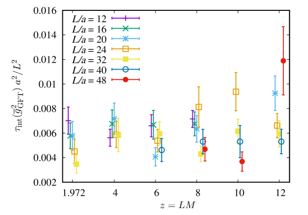
Figure 7: Integrated autocorrelation times $\tau_{\rm int}({\overline{g}}_{\rm GFT}^{2})$ of the gradient flow coupling in units of measurements (every five trajectories, i.e., 10 MDUs) scaled with $a^{2}/L^{2}$ vs. the dimensionless quantity $z=LM$ of our massive simulations. The points are slightly shifted from actual $z$ values for better visibility.

Appendix D Mistuning Corrections

To correct the mistuning of the LCP, the slope

$$S=\left.\frac{\partial\overline{g}_{\rm GF}^{2}}{\partial\tilde{g}_{0}^{2}}\right|_{L/a}=\frac{\overline{g}_{\rm GF}\beta^{(3)}_{\rm GF}(\overline{g}_{\rm GF})}{g_{0}\beta^{(3)}_{0}(g_{0})}+{\rm O}(a^{2})\,,$$ (D.123)

is required. To compute it, the non-perturbative $\beta_{\rm GF}$-function of the gradient flow coupling at $\overline{g}_{\rm GF}^{2}=3.949$ and the non-perturbative bare $\beta_{0}$-function at the bare couplings of our LCP are needed. The first has been determined to high precision in [35] and is given by

$$\beta_{\rm GF}^{(3)}(\sqrt{3.949})=-0.471\pm 0.004\,.$$ (D.124)

The bare $\beta_{0}$-function can be estimated by parameterizing the $L/a\geq 20$ data in the first two columns of table 1 according to

$$\ln\left(\frac{L}{a}\right)\approx{\rm const.}+\frac{1}{2k_{3}g_{0}^{2}}\,,$$ (D.125)

the $\beta_{0}$ function in this short range of couplings is then given by

$$\beta_{0}^{(3)}\approx-k_{3}g_{0}^{3},\qquad\text{with}\qquad k_{3}=0.054\,.$$ (D.126)

With this slope the $\beta_{\rm LCP}$ values in the last column of table 1 are determined. From these then the desired simulation parameters for the massive runs follow, as described in section 4.2.

In practice, the massive runs were performed at slightly different parameters, and need to be corrected as well. The relevant slope here is given by the dependence of the massive coupling on the bare one

$$\left.\frac{\partial{\overline{g}}_{\rm GFT}^{2}}{\partial\tilde{g}_{0}^{2}}\right|_{z,L/a}=\left.\frac{\partial{\overline{g}}_{\rm GFT}^{2}}{\partial\ln(L)}\right|_{z,L/a}\left(\frac{{\rm d}\tilde{g}_{0}^{2}}{{\rm d}\,\ln(a)}\right)^{-1}\,.$$ (D.127)

The last factor is again related to the bare $\beta_{0}$-function, and the same parameterization as above can be used. The first factor, however, has never been determined but can be approximated based on decoupling. Matching of the three-flavor and the pure gauge theories means, that $\Lambda^{(0)}(M)=\Lambda^{(3)}\,P(M/\Lambda^{(3)})$. For physical couplings in the continuum limit we then have

$$[{\overline{g}}_{\rm GFT}^{(3)}(L,z)]^{2}=[{\overline{g}}_{\rm GFT}^{(0)}(L)]^{2}+{\rm O}(z^{-2}).$$ (D.128)

The $N_{\mathrm{f}}=0$ coupling and $\Lambda^{(0)}$ are related

$$[{\overline{g}}_{\rm GFT}^{(0)}(L)]^{2} = F(L\Lambda^{(0)})$$ (D.129)

$$= F\left(L\Lambda^{(3)}P\left(\frac{z}{L\Lambda^{(3)}}\right)\right)$$ (D.130)

$$= [{\overline{g}}_{\rm GFT}^{(3)}(L,z)]^{2}+{\rm O}(z^{-2})\,.$$ (D.131)

The exact form of the function $F$ will not be needed, but it is essentially the inverted relation eq. (2.4) together with a scheme change of the $\Lambda$ parameter. Taking the $L$-derivative of the second line and then using decoupling to express everything in terms of $N_{\mathrm{f}}=0$ quantities results in

$$L\frac{\partial[{\overline{g}}_{\rm GFT}^{(3)}]^{2}}{\partial L}=-2{\overline{g}}_{\rm GFT}^{(0)}\beta^{(0)}_{\rm GFT}({\overline{g}}_{\rm GFT}^{(0)})\left(1-\eta^{M}\right)+{\rm O}(z^{-2})\,,$$ (D.132)

with $\eta^{M}=\frac{M}{P}\,\left.\frac{\partial P}{\partial M}\right|_{\Lambda^{(3)}}=2/11+{\rm O}(\alpha(m_{\star}))$, where the ${\rm O}(\alpha(m_{\star}))$ corrections are very small [28] and can safely be dropped.

The shifts are applied to couplings at finite $z$ and finite $a$. The leading corrections to the $z\to\infty$, $a\to 0$ limit are built into the extrapolation formulae eq. (4.64) and eq. (4.69), which is why $p_{1}$, $p_{2}$ and $B$ are known in

$$[{\overline{g}}_{\rm GFT}^{(3)}]^{2} = F\left(L\Lambda^{(3)}_{\rm eff}P\left(\frac{z}{L\Lambda^{(3)}_{\rm eff}}\right)\right)+(p_{1}+p_{2}z^{2})\frac{a^{2}}{L^{2}}\,,$$ (D.133)

$$\Lambda^{(3)}_{\rm eff} = \Lambda^{(3)}+\frac{B}{z^{2}}\,.$$ (D.134)

The $L$-derivative of the coupling at finite $z$ and $a$ has then corrections $R_{\rm a}$ and $R_{\rm z}$ of the form

$$L\frac{\partial[{\overline{g}}_{\rm GFT}^{(3)}]^{2}}{\partial L}=-2{\overline{g}}_{\rm GFT}^{(0)}\beta^{(0)}_{\rm GFT}({\overline{g}}_{\rm GFT}^{(0)})\left(1-\eta^{M}\right)\left[1+R_{\rm z}+R_{\rm a}\right]\,,$$ (D.135)

which to leading order are given by

$$R_{\rm z} \approx \frac{B/\Lambda}{z^{2}}4[{\overline{g}}_{\rm GFT}^{(0)}]^{2}\,k_{0}\,,$$ (D.136)

$$R_{\rm a} \approx \frac{-2(p_{1}+p_{2}z^{2})\frac{a^{2}}{L^{2}}}{-2{\overline{g}}_{\rm GFT}^{(0)}\beta^{(0)}_{\rm GFT}({\overline{g}}_{\rm GFT}^{(0)}\left(1-\eta^{M}\right)}\,.$$ (D.137)

Finally, $k_{0}$ parameterizes the $\beta^{(0)}_{\rm GFT}$-function in the relevant range of couplings

$$\beta^{(0)}_{\rm GFT}({\overline{g}}_{\rm GFT})\approx-k_{0}\,{\overline{g}}_{\rm GFT}^{3}\,.$$ (D.138)

Its value is $0.079$ and $0.076$ for $c=0.3$ and $c=0.36$, respectively.

Appendix E Mass renormalization

To compute the strong coupling from decoupling relations, simulations at constant renormalized mass are necessary. This appendix describes, how a given value of the RGI quark mass in GeV translates into a hopping parameter at a given $\beta$ value.

In a first step the RGI mass $M$ is translated into a renormalized mass $\overline{m}(\mu_{\rm dec})$ in the SF scheme

$$\overline{m}(\mu_{\rm dec})=M\times\frac{\overline{m}(\mu_{0}/2)}{M}\times\frac{\overline{m}(\mu_{\rm dec})}{\overline{m}(\mu_{0}/2)}\,.$$ (E.139)

Here ${M}/{\overline{m}(\mu_{0}/2)}=1.7505(89)$ has been determined in [24] for a scale $\mu_{0}$ defined by $\overline{g}^{2}_{\rm SF}(\mu_{0})=2.0120$, which corresponds to $\overline{g}_{\rm GF}^{2}(\mu_{0}/2)=2.6723(64)$. For the (short) running of the mass

$$\frac{\overline{m}(\mu_{\rm dec})}{\overline{m}(\mu_{0}/2)}=\exp\left\{-\int\limits_{\overline{g}(\mu_{\rm dec})}^{\overline{g}(\mu_{0}/2)}\frac{\tau(x)}{\beta(x)}\,dx\right\}\,,$$ (E.140)

a parametrization of non-perturbatively determined [24] $\tau/\beta$ data is used

$$\frac{\tau(\overline{g}_{\rm GF})}{\beta(\overline{g}_{\rm GF})}=\frac{1}{\overline{g}_{\rm GF}}\left(f_{0}+f_{1}\overline{g}_{\rm GF}^{2}+f_{2}\overline{g}_{\rm GF}^{4}+f_{3}\overline{g}_{\rm GF}^{6}\right)\,,$$ (E.141)

with $f_{0}=1.28493,f_{1}=-0.292465,f_{2}=0.0606401,f_{3}=-0.00291921$. The parameters are correlated, namely

$$\begin{split}{\rm cov}(f_{i},f_{j})=&\left({\footnotesize\begin{array}[]{cccc}\phantom{+}2.33798\times 10^{-2}&-1.47011\times 10^{-2}&\phantom{+}2.81966\times 10^{-3}&-1.66404\times 10^{-4}\\ -1.47011\times 10^{-2}&\phantom{+}9.54563\times 10^{-3}&-1.87752\times 10^{-3}&\phantom{+}1.12962\times 10^{-4}\\ \phantom{+}2.81966\times 10^{-3}&-1.87752\times 10^{-3}&\phantom{+}3.78680\times 10^{-4}&-2.32927\times 10^{-5}\\ -1.66404\times 10^{-4}&\phantom{+}1.12962\times 10^{-4}&-2.32927\times 10^{-5}&\phantom{+}1.46553\times 10^{-6}\\ \end{array}}\right)\,.\end{split}$$ (E.142)

This allows to obtain

$$\frac{M}{\overline{m}(\mu_{\mathrm{dec}})}=1.474(11).$$ (E.143)

This renormalized mass can then be related to either the bare subtracted quark mass $m_{\rm q}(g_{0}^{2},m_{0})=m_{0}-m_{\rm crit}(g_{0}^{2})$ or to the bare PCAC mass $m_{\rm PCAC}(g_{0}^{2},m_{0})$.

$$\overline{m}(\mu_{\rm dec}) = m_{\rm PCAC}(g_{0}^{2},m_{0})\frac{Z_{\rm A}(\tilde{g}_{0}^{2})}{Z_{\rm P}(\tilde{g}_{0}^{2},a\mu_{\rm dec})}\left[1+(b_{\rm A}(g_{0}^{2})-b_{\rm P}(g_{0}^{2}))am_{\rm q}(g_{0}^{2},m_{0})\right]$$ (E.144)

$$= m_{\rm q}(g_{0}^{2},m_{0})Z_{\rm m}(\tilde{g}_{0}^{2},a\mu_{\rm dec})\left[1+b_{\rm m}(g_{0}^{2})am_{\rm q}(g_{0}^{2},m_{0})\right]\,,$$ (E.145)

valid only up to cutoff effects of $O(a^{2})$ with the improved bare coupling [58]

$$\tilde{g}_{0}^{2}=g_{0}^{2}\left(1+b_{\rm g}(g_{0}^{2})am_{\rm q}\right)\,.$$ (E.146)

The second relation is more useful, since it connects $\overline{m}$ directly to the simulation parameter $\kappa$: $am_{\rm q}=am_{0}-am_{\rm crit}(g_{0}^{2})=\frac{1}{2\kappa}-\frac{1}{2\kappa_{c}}$. On the other hand, the renormalization factors in the first relation are easier to compute, or already known. The missing piece is then the relation between $m_{\rm PCAC}$ and $m_{\rm q}$,

$$m_{\rm PCAC}(g_{0}^{2},m_{0})=$$ (E.147)

$$\;\underbrace{\frac{Z_{\rm P}(\tilde{g}_{0}^{2},a\mu_{\rm dec})Z_{\rm m}(\tilde{g}_{0}^{2},a\mu_{\rm dec})}{Z_{\rm A}(\tilde{g}_{0}^{2})}}_{\equiv\hat{Z}(\tilde{g}_{0}^{2})}m_{\rm q}(g_{0}^{2},m_{0})\left[1+\underbrace{[b_{\rm m}(g_{0}^{2})+b_{\rm P}(g_{0}^{2})-b_{\rm A}(g_{0}^{2})]}_{\equiv\hat{b}(g_{0}^{2})}am_{\rm q}(g_{0}^{2},m_{0})\right]\,,$$

with renormalization factor $\hat{Z}(\tilde{g}_{0}^{2})$ and improvement coefficient $\hat{b}(g_{0}^{2})$, which can both be obtained non-perturbatively from our close-to-massless simulations. More precisely, since these runs vary $m_{0}$ around $m_{\rm crit}$ while keeping $g_{0}$ constant (instead of $\tilde{g}_{0}$), what we have access to are $\hat{Z}$ and $\hat{b}^{\rm eff}$ in

$$m_{\rm PCAC}(g_{0}^{2},m_{0})=\hat{Z}(g_{0}^{2})m_{\rm q}(g_{0}^{2},m_{0})\left[1+\underbrace{\left(\hat{b}(g_{0}^{2})+g_{0}^{2}b_{\rm g}(g_{0}^{2})\frac{\hat{Z}^{\prime}(g_{0}^{2})}{\hat{Z}(g_{0}^{2})}\right)}_{\equiv\hat{b}^{\rm eff}(g_{0}^{2})}am_{\rm q}(g_{0}^{2},m_{0})\right]\,.$$ (E.148)

First, we perform a simultaneous linear fit to the data in table 12 at fixed $L/a$

$$Lm_{\rm PCAC} = c_{0}+c_{1}Lm_{0}+c_{2}(Lm_{0})^{2}$$ (E.149)

$$Z_{\rm P} = c_{3}+c_{4}Lm_{0}+c_{5}(Lm_{0})^{2}$$ (E.150)

$$\overline{g}_{\rm GF}^{2} = c_{6}+c_{7}Lm_{0}+c_{8}(Lm_{0})^{2}\,.$$ (E.151)

Then $am_{\rm crit}$, $\hat{Z}$, $\hat{b}^{\rm eff}$, $Z_{\rm P}$, $\overline{g}_{\rm GF}^{2}$ and ${\rm d}\,\overline{g}_{\rm GF}^{2}/{\rm d}\,am_{0}$ at zero quark mass, as well as their covariances are obtained from the fit parameters $c_{i}$. The results of these fits can be found in Table 13.

$L/a$	$\beta$	$am_{\rm crit}$	$\hat{Z}$	$\hat{b}^{\rm eff}$	$Z_{P}$	$Z_{A}$
12	4.3020	-0.323417(38)	1.1707(31)	-0.408(26)	0.57708(82)	0.8322(26)
16	4.4662	-0.312928(23)	1.1613(22)	-0.486(29)	0.56759(82)	0.8432(34)
20	4.5997	-0.304289(24)	1.1492(28)	-0.461(39)	0.5628(15)	0.8515(41)
24	4.7141	-0.296941(14)	1.1455(12)	-0.497(18)	0.5554(17)	0.8582(47)
32	4.9000	-0.285427(12)	1.1374(13)	-0.608(45)	0.5446(35)	0.8681(55)
40	5.0671	-0.275473(11)	1.1259(12)	-0.490(19)	0.5459(42)	0.8762(62)
48	5.1739	-0.2693605(82)	1.1233(10)	-0.517(17)	0.5427(49)	0.8810(66)

Table 13: Results for $am_{\rm crit}$, $\hat{Z},\hat{b}^{\rm eff}$ and $Z_{P}$ from fits and extrapolations of $Z_{A}$.

To read off $\hat{Z}^{\prime}/\hat{Z}$ to compute $\hat{b}$ from $\hat{b}^{\rm eff}$, and to obtain the value $am_{\rm crit}(g_{0}^{2})$ from data at slightly shifted $\tilde{g}_{0}^{2}$, we carry out another linear fit of the results in table 13

$$am_{\rm crit} = d_{0}+d_{1}g_{0}^{2}+d_{2}g_{0}^{4}+d_{3}g_{0}^{6}$$ (E.152)

$$\hat{Z} = d_{4}+d_{5}g_{0}^{2}+d_{6}g_{0}^{4}\,.$$ (E.153)

The result is shown in Fig. 8, asymptotic PT behavior is not built into these fits.

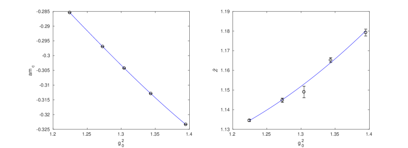
Figure 8: Critical mass and $\hat{Z}$ as a function of $g_{0}^{2}$.

The axial current renormalization $Z_{\rm A}$ was computed very precisely based on universal relations between correlators in a chirally rotated Schrödinger Functional [102]. The calculation was carried out at the $\beta$ values at which also the large volume CLS simulations are carried out. These are coarser lattices, than the ones needed here, which means that an extrapolation of the data is necessary. A fit, with restriction to 1-loop perturbation theory for $g_{0}\to 0$, as proposed by the authors is

$$Z_{\rm A}=1-0.090488g_{0}^{2}+c_{1}g_{0}^{4}+c_{2}g_{0}^{6}+c_{3}g_{0}^{8}\,,$$ (E.154)

with $c_{1}=0.127163,c_{2}=-0.178785,c_{3}=0.051814$ and

$${\rm cov}(c_{i},c_{j})=10^{-2}\times\begin{pmatrix}0.29841165&-0.36050066&0.10868891\\ -0.36050066&0.43567202&-0.13140137\\ 0.10868891&-0.13140137&0.03964605\end{pmatrix}\,.$$ (E.155)

The right column of table 13 lists the extrapolated renormalization factors at the necessary $\beta$ values, see also figure 9.

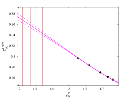
Figure 9: Extrapolations of $Z_{\rm A}$.

With known $Z_{\rm A}$, $Z_{\rm P}$ and $\hat{Z}$, the $\\ ZmZm$ in the relation between the bare and the renormalized mass is determined non-perturbatively. The only missing pieces are the improvement coefficients $b_{\rm A}$, $b_{\rm P}$ and $b_{\rm g}$, for which we take their 1 loop approximations [60, 103, 104]

$$b_{\rm A} = \phantom{-}\,1+0.0881(13)\times C_{\rm F}\ g_{0}^{2}\,,$$ (E.156)

$$b_{\rm P} = \phantom{-}\,1+0.0889(14)\times C_{\rm F}\ g_{0}^{2}\,,$$ (E.157)

$$b_{\rm m} = -\frac{1}{2}-0.0576(11)\times C_{\rm F}\ g_{0}^{2}\,,$$ (E.158)

$$b_{\rm g} = \phantom{-}\,0+0.012000(2)\times N_{\mathrm{f}}\ g_{0}^{2}\,.$$ (E.159)

The perturbative result for $b_{\rm m}$ will not be used, except for testing PT, $b_{\rm m}$ is instead obtained as $b_{\rm m}=\hat{b}-b_{\rm P}+b_{\rm A}$.

If $\tilde{g}_{0}$ denotes the bare coupling of the LCP defined by $\overline{m}=0,\overline{g}_{\rm GF}^{2}=3.949$, then the massive simulations need to be carried out at a slightly different bare coupling, in order to keep $\tilde{g}_{0}$ and hence the volume constant. If we denote this slightly shifted coupling by $g_{0}^{2}$, we find that the bare parameters of the massive simulation, $g_{0}^{2}$ and $m_{0}$, have to be chosen such that

$$g_{0}^{2} = \tilde{g}_{0}^{2}\left(1-b_{\rm g}(\tilde{g}_{0}^{2})am_{\rm q}(g_{0}^{2},m_{0})\right)$$ (E.160)

$$L\overline{m}(\mu_{\rm dec}) = Lm_{\rm q}(g_{0}^{2},m_{0})Z_{\rm m}(\tilde{g}_{0}^{2})\left[1+b_{\rm m}(\tilde{g}_{0}^{2})am_{\rm q}(g_{0}^{2},m_{0})\right]\,$$ (E.161)

hold. Note that $b_{x}(g_{0}^{2})am_{\rm q}=b_{x}(\tilde{g}_{0}^{2})am_{\rm q}+O(a^{2})$ was used to derive these expressions. These equations can be explicitly solved for the simulation parameters in three steps

$$am_{\rm q} = \frac{1}{2b_{\rm m}}\left(\pm\sqrt{1+\frac{4b_{\rm m}L\overline{m}}{L/a\ Z_{\rm m}}}-1\right)\,,$$ (E.162)

$$g_{0}^{2} = \tilde{g}_{0}^{2}/\left(1+b_{\rm g}am_{\rm q}\right)\,$$ (E.163)

$$am_{0} = am_{\rm q}+am_{\rm crit}(g_{0}^{2})\,.$$ (E.164)

The uncertainties in all quantities entering these equations are known, which means that we know the precision of the massive simulation parameters, and conversely we control the precision that we can expect to reach for $z$. How an error on $z$ propagates into the determination of $\Lambda$ is discussed below, but first, let us consider a cross-check of demonstrating that $z$ is fixed correctly. Once the massive simulations have been carried out, we measure the PCAC masses and compute

$$\tilde{z}=Lm_{\rm PCAC}\frac{M}{\bar{m}(\mu)}\frac{Z_{\rm A}(\tilde{g}_{0}^{2})}{Z_{\rm P}(\tilde{g}_{0}^{2},a\mu)}[1+(b_{\rm A}-b_{\rm P})am_{\rm q}]=z+{\rm O}(a^{2})$$ (E.165)

The results are shown in figure 10. The precision is satisfactory, and the ${\rm O}(a^{2})$ effects are reasonably small.

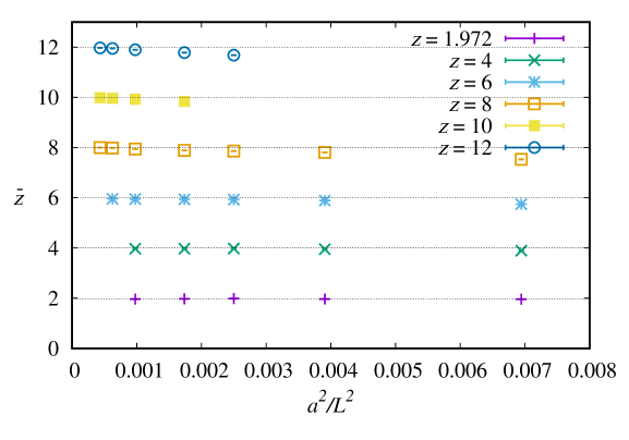
Figure 10: Overview of our massive simulations for $M=1.6\ldots 9.5$ GeV, $T=2L$, showing the dimensionless RGI mass $\tilde{z}$, eq. (E.165) which agrees well with the input $z$-values prescribed in terms of the bare mass $m_{\rm q}$.

Appendix F Propagating the error of $z$

One would like to estimate which precision is necessary in fixing $M$ in order to achieve a certain precision in $\overline{g}_{\rm GF}^{2}(\mu,M)$ and then in $\Lambda^{(3)}$ obtained from $\Lambda^{(0)}$.

The most relevant place where an uncertainty in $M$ matters is the $P$ function (to be precise $P_{0,3}$ in the notation of [28]), which relates the $\Lambda$ parameters as

$$\Lambda^{(0)}_{\overline{\rm MS}}=P(M/\Lambda^{(3)}_{\overline{\rm MS}})\,\Lambda^{(3)}_{\overline{\rm MS}}\,.$$ (F.166)

One can simply use this noting that

$$\left.M\partial_{M}\Lambda^{(3)}_{\overline{\rm MS}}\right|_{\Lambda^{(0)}_{\overline{\rm MS}}}=M\partial_{M}\frac{\Lambda^{(0)}_{\overline{\rm MS}}}{P(M/\Lambda^{(3)}_{\overline{\rm MS}})}=-\Lambda^{(3)}_{\overline{\rm MS}}\eta^{M}\,,$$ (F.167)

and insert the known perturbation theory for $\eta^{M}=\frac{M}{P}\partial_{M}P$. The function $\eta^{M}$ is known to 4 loops and the first two perturbative terms are (cf. [28])

$$\eta^{M}\sim\frac{6}{33}+\frac{1926}{(4\pi)^{2}33^{2}}g_{\star}^{2}+\ldots\,,$$ (F.168)

where $g_{\star}=\bar{g}_{{\rm\overline{MS\kern-0.35002pt}\kern 0.35002pt}}(m_{\star})$ and $\overline{m}_{{\rm\overline{MS\kern-0.35002pt}\kern 0.35002pt}}(m_{\star})=m_{\star}$. This is enough to estimate the required precision in the tuning of $M$.

Another place where $M$ mistunings need to be accounted for, is the continuum extrapolation of the massive coupling. To propagate the $M$ uncertainty onto $\bar{g}^{2}$, its derivative with respect to the mass must be known.

For this we are going to use the fundamental formula Eq. (2.10)

$${\Lambda^{(3)}_{\overline{\rm MS}}}=\mu_{\rm dec}\times\varphi_{\rm GF}^{(0)}(\bar{g}_{\rm GF})\times\frac{\Lambda^{(0)}_{\overline{\rm MS}}}{\Lambda^{(0)}_{\rm GF}}\times P(M/\Lambda^{(3)}_{\overline{\rm MS}})\,.$$ (F.169)

where ${\bar{g}_{\rm GF}^{2}}$ is the massive coupling in the GF scheme in Eq. (2.11). First note that

$$\varphi_{\rm GF}^{(0)}({\bar{g}_{\rm GF}})=\exp\left\{-\int^{\bar{g}_{\rm GF}}\frac{{\rm d}x}{\beta_{\rm GF}^{(0)}(x)}\right\}\times\text{constant}\,,$$ (F.170)

with $z=M/\mu_{\rm dec}$ only appearing in the first term. Now we can take the logarithm

$$\log\Lambda_{\overline{\rm MS}}^{(3)}=-\int^{\bar{g}_{\rm GF}}\frac{{\rm d}x}{\beta_{\rm GF}^{(0)}(x)}+\log(P(\mu_{\rm dec}z/\Lambda_{\overline{\rm MS}}^{(3)}))+\text{$z$ independent terms}\,.$$ (F.171)

Taking a derivative with respect to $z$ gives

$$\frac{\partial\bar{g}_{\rm GF}}{\partial z}=-\beta_{\rm GF}^{(0)}(\bar{g}_{\rm GF})\partial_{z}\log P$$ (F.172)

and finally

$$\frac{\partial\bar{g}_{\rm GF}^{2}}{\partial z}=\frac{\eta^{M}}{z}\times(-2\bar{g}_{\rm GF}\beta_{\rm GF}^{(0)}(\bar{g}_{\rm GF}))\,,$$ (F.173)

where we have used $\partial_{z}\log P=\eta^{M}/z$.

Figs. 11 show the results. The derivative is not that small, especially at $z=4$ ($z=2$ is irrelevant).

Figure 11: (a) The derivative $\partial_{z}\log P=\eta^{M}/z$. (b) The full derivative of the coupling Eq. (F.173).

Numerically we find with excellent approximation that

$$z\partial_{z}\log P\approx 0.19$$ (F.174)

so that we will use for the error propagation the formula

$$\frac{1}{\bar{g}_{\rm GF}^{2}}\frac{\partial\bar{g}^{2}_{\rm GF}}{\partial z}=-\frac{0.38}{z\bar{g}_{\rm GF}}\beta_{\rm GF}^{(0)}(\bar{g}_{\rm GF})\,,$$ (F.175)

so that

$${\delta\bar{g}_{\rm GF}^{2}}={0.38}{\bar{g}_{\rm GF}}\beta_{\rm GF}^{(0)}(\bar{g}_{\rm GF})\frac{\delta z}{z}\,.$$ (F.176)

Finally, note that the massive coupling $\bar{g}_{\text{GFT}}^{2}$ is different from $\bar{g}_{\rm GF}^{2}$ (because of $T=2L$, the mass effects and possibly the different values of $c$). The relation between couplings is known non-perturbatively in the region of interest for the $N_{\rm f}=0$ case

$$\frac{1}{\bar{g}_{\text{GFT}}^{2}}-\frac{1}{\bar{g}_{\rm GF}^{2}}=f(\bar{g}_{\rm GF})\,,$$ (F.177)

see Eq. (B.106). Neglecting $1/z^{2}$ terms, we have that

$$\delta\bar{g}_{\text{GFT}}^{2}=\left(\frac{1}{\bar{g}_{\rm GF}^{4}}-f^{\prime}(\bar{g}_{\rm GF})\right)\bar{g}_{\text{GFT}}^{4}{0.38}{\bar{g}_{\rm GF}}\beta_{\rm GF}^{(0)}(\bar{g}_{\rm GF})\frac{\delta z}{z}\,.$$ (F.178)

In practice $f^{\prime}(\bar{g}_{\rm GF})\approx 0$, and the whole uncertainty $\delta\bar{g}_{\text{GFT}}^{2}$ is well below the statistical uncertainty of $\bar{g}_{\text{GFT}}^{2}$. The uncertainty $\delta z$ contributes less than a 0.2% to the final error squared in $\Lambda_{\overline{\rm MS}}^{(3)}$.

Appendix G Line of constant physics for $L/a=40,48$

For $L/a>32$ we do not have direct simulations to fix our line of constant physics $\bar{g}^{2}_{\rm GF}(\mu_{\rm dec},a\mu_{\rm dec})=3.949$. For the case $a\mu_{\rm dec}=1/48$, we first determine the inverse lattice step scaling function from the data available in the literature [35], in particular for the fit used in [35] for the $\beta$-function. The result of such determination is

$$\Sigma^{-1}(3.95,a\mu_{\rm dec}=1/24)=2.9951(62)\,.$$ (G.179)

Now we determine the value of $\beta$ for $a\mu_{\rm dec}=1/24$ such that the coupling equals 2.9951. This can be determined by interpolating the data of table 14 using as fit ansatze

$$1/\bar{g}^{2}_{\rm GF}-\beta/6=P_{3}(\beta)\,,$$ (G.180)

where $P_{3}(x)$ is a third degree polynomial. The result of this procedure is

$$\beta=5.1742(58)\qquad(L/a=48)\,.$$ (G.181)

s.t. the coupling for $L/a=48$ would be exactly $3.95$. Note that this value has to be slightly corrected to the true LCP $\bar{g}^{2}_{\rm GF}(\mu_{\rm dec})=3.949$ (see table 1).

Finally, the values of table 1 with $L/a\leq 32$, together with this last determination can be used to interpolate the value of $\beta$ s.t. $\bar{g}^{2}_{\rm GF}=3.949$ for $L/a=40$. We choose as fit functional

$$\log(L/a)=P_{4}(\beta)\,,$$ (G.182)

where $P_{4}(x)$ is a fourth degree polynomial. The resulting value is

$$\beta=5.0497(41)\qquad(L/a=40)\,.$$ (G.183)

$\beta$	$\bar{g}^{2}_{\rm GF}$	$1/g^{2}_{\rm GF}-\beta/6$
5.543070	2.5043(76)	-0.5245(12)
5.242465	2.8963(87)	-0.5285(10)
4.938726	3.403(11)	-0.52930(95)
4.634654	4.180(14)	-0.53319(81)
4.331660	5.380(25)	-0.53609(85)
4.128217	6.785(36)	-0.54065(78)

Table 14: Simulations with $L/a=24$ used to interpolate the vaulue $\bar{g}^{2}_{\rm GF}=2.9951$.

References

- [1] ALPHA Collaboration, M. Dalla Brida, R. Höllwieser, F. Knechtli, T. Korzec, A. Ramos, and R. Sommer, “Non-perturbative renormalization by decoupling,” Phys. Lett. B 807 (2020) 135571, arXiv:1912.06001 [hep-lat].
- [2] M. Dalla Brida and A. Ramos, “The gradient flow coupling at high-energy and the scale of SU(3) Yang-Mills theory,” Eur. Phys. J. C79 no. 8, (2019) 720, arXiv:1905.05147 [hep-lat].
- [3] A. Nada and A. Ramos, “An analysis of systematic effects in finite size scaling studies using the gradient flow,” Eur. Phys. J. C 81 no. 1, (2021) 1, arXiv:2007.12862 [hep-lat].
- [4] Y. Aoki et al., “FLAG Review 2021,” arXiv:2111.09849 [hep-lat].
- [5] ALPHA Collaboration, M. Bruno, M. Dalla Brida, P. Fritzsch, T. Korzec, A. Ramos, S. Schaefer, H. Simma, S. Sint, and R. Sommer, “QCD Coupling from a Nonperturbative Determination of the Three-Flavor Parameter,” Phys. Rev. Lett. 119 no. 10, (2017) 102001, arXiv:1706.03821 [hep-lat].
- [6] ATLAS Collaboration , https://atlas.web.cern.ch/Atlas/GROUPS/PHYSICS/PUBNOTES/ATL-PHYS-PUB-2019-024/ .
- [7] Particle Data Group Collaboration, P. A. Zyla et al., “Review of Particle Physics,” PTEP 2020 no. 8, (2020) 083C01.
- [8] Flavour Lattice Averaging Group Collaboration, S. Aoki et al., “FLAG Review 2019,” Eur. Phys. J. C80 no. 2, (2020) 113, arXiv:1902.08191 [hep-lat].
- [9] L. Del Debbio and A. Ramos, “Lattice determinations of the strong coupling,” Physics Reports 920 (2021) 1–71, arXiv:2101.04762 [hep-lat].
- [10] M. Dalla Brida, “Past, present, and future of precision determinations of the QCD parameters from lattice QCD,” Eur. Phys. J. A 57 no. 2, (2021) 66, arXiv:2012.01232 [hep-lat].
- [11] ALPHA Collaboration, M. Dalla Brida, P. Fritzsch, T. Korzec, A. Ramos, S. Sint, and R. Sommer, “Determination of the QCD -parameter and the accuracy of perturbation theory at high energies,” Phys. Rev. Lett. 117 no. 18, (2016) 182001, arXiv:1604.06193 [hep-ph].
- [12] ALPHA Collaboration, M. Dalla Brida, P. Fritzsch, T. Korzec, A. Ramos, S. Sint, and R. Sommer, “A non-perturbative exploration of the high energy regime in QCD,” Eur. Phys. J. C78 no. 5, (2018) 372, arXiv:1803.10230 [hep-lat].
- [13] M. Lüscher, P. Weisz, and U. Wolff, “A Numerical method to compute the running coupling in asymptotically free theories,” Nucl.Phys. B359 (1991) 221–243.
- [14] M. Lüscher, R. Sommer, P. Weisz, and U. Wolff, “A Precise determination of the running coupling in the SU(3) Yang-Mills theory,” Nucl. Phys. B 413 (1994) 481–502, arXiv:hep-lat/9309005.
- [15] E. I. Bribian, J. L. D. Golan, M. G. Perez, and A. Ramos, “Memory efficient finite volume schemes with twisted boundary conditions,” Eur. Phys. J. C 81 no. 10, (2021) 951, arXiv:2107.03747 [hep-lat].
- [16] ALPHA Collaboration, M. Della Morte, R. Frezzotti, J. Heitger, J. Rolf, R. Sommer, and U. Wolff, “Computation of the strong coupling in QCD with two dynamical flavors,” Nucl. Phys. B713 (2005) 378–406, arXiv:hep-lat/0411025 [hep-lat].
- [17] P. Fritzsch, F. Knechtli, B. Leder, M. Marinkovic, S. Schaefer, R. Sommer, and F. Virotta, “The strange quark mass and Lambda parameter of two flavor QCD,” Nucl. Phys. B 865 (2012) 397–429, arXiv:1205.5380 [hep-lat].
- [18] PACS-CS Collaboration, S. Aoki et al., “Precise determination of the strong coupling constant in = 2+1 lattice QCD with the Schrodinger functional scheme,” JHEP 10 (2009) 053, arXiv:0906.3906 [hep-lat].
- [19] ALPHA Collaboration, F. Tekin, R. Sommer, and U. Wolff, “The Running coupling of QCD with four flavors,” Nucl. Phys. B840 (2010) 114–128, arXiv:1006.0672 [hep-lat].
- [20] P. Perez-Rubio and S. Sint, “Non-perturbative running of the coupling from four flavour lattice QCD with staggered quarks,” PoS LATTICE2010 (2010) 236, arXiv:1011.6580 [hep-lat].
- [21] R. Sommer and U. Wolff, “Non-perturbative computation of the strong coupling constant on the lattice,” Nucl. Part. Phys. Proc. 261-262 (2015) 155–184, arXiv:1501.01861 [hep-lat].
- [22] D. Nogradi and A. Patella, “Strong dynamics, composite Higgs and the conformal window,” Int. J. Mod. Phys. A 31 no. 22, (2016) 1643003, arXiv:1607.07638 [hep-lat].
- [23] T. DeGrand, “Lattice tests of beyond Standard Model dynamics,” Rev. Mod. Phys. 88 (2016) 015001, arXiv:1510.05018 [hep-ph].
- [24] ALPHA Collaboration, I. Campos, P. Fritzsch, C. Pena, D. Preti, A. Ramos, and A. Vladikas, “Non-perturbative quark mass renormalisation and running in QCD,” Eur. Phys. J. C78 no. 5, (2018) 387, arXiv:1802.05243 [hep-lat].
- [25] ALPHA Collaboration, I. Campos, M. Dalla Brida, G. M. de Divitiis, A. Lytle, M. Papinutto, L. Pirelli, and A. Vladikas, “Nonperturbative running of the quark mass for QCD from the chirally rotated Schrödinger functional,” Phys. Rev. D 105 no. 5, (2022) 054506, arXiv:2112.10606 [hep-lat].
- [26] T. Appelquist and J. Carazzone, “Infrared Singularities and Massive Fields,” Phys. Rev. D11 (1975) 2856.
- [27] S. Weinberg, “Effective Gauge Theories,” Phys. Lett. 91B (1980) 51–55.
- [28] ALPHA Collaboration, A. Athenodorou, J. Finkenrath, F. Knechtli, T. Korzec, B. Leder, M. Krstic Marinkovic, and R. Sommer, “How perturbative are heavy sea quarks?,” Nucl. Phys. B943 (2019) 114612, arXiv:1809.03383 [hep-lat].
- [29] W. Bernreuther and W. Wetzel, “Decoupling of Heavy Quarks in the Minimal Subtraction Scheme,” Nucl. Phys. B197 (1982) 228–236. [Erratum: Nucl. Phys.B513,758(1998)].
- [30] A. G. Grozin, M. Hoeschele, J. Hoff, M. Steinhauser, M. Hoschele, J. Hoff, and M. Steinhauser, “Simultaneous decoupling of bottom and charm quarks,” JHEP 09 (2011) 066, arXiv:1107.5970 [hep-ph].
- [31] K. G. Chetyrkin, J. H. Kühn, and C. Sturm, “QCD decoupling at four loops,” Nucl. Phys. B744 (2006) 121–135, arXiv:hep-ph/0512060 [hep-ph].
- [32] Y. Schröder and M. Steinhauser, “Four-loop decoupling relations for the strong coupling,” JHEP 01 (2006) 051, arXiv:hep-ph/0512058 [hep-ph].
- [33] B. A. Kniehl, A. V. Kotikov, A. I. Onishchenko, and O. L. Veretin, “Strong-coupling constant with flavor thresholds at five loops in the anti-MS scheme,” Phys. Rev. Lett. 97 (2006) 042001, arXiv:hep-ph/0607202.
- [34] M. Gerlach, F. Herren, and M. Steinhauser, “Wilson coefficients for Higgs boson production and decoupling relations to ,” JHEP 11 (2018) 141, arXiv:1809.06787 [hep-ph].
- [35] ALPHA Collaboration, M. Dalla Brida, P. Fritzsch, T. Korzec, A. Ramos, S. Sint, and R. Sommer, “Slow running of the Gradient Flow coupling from 200 MeV to 4 GeV in QCD,” Phys. Rev. D95 no. 1, (2017) 014507, arXiv:1607.06423 [hep-lat].
- [36] P. Fritzsch, J. Heitger, and S. Kuberski, “ improved quark mass renormalization for a non-perturbative matching of HQET to three-flavor QCD,” PoS LATTICE2018 (2018) 218, arXiv:1811.02591 [hep-lat].
- [37] S. Weinberg, “New approach to the renormalization group,” Phys. Rev. D 8 (1973) 3497–3509.
- [38] M. Lüscher, R. Narayanan, P. Weisz, and U. Wolff, “The Schrodinger functional: A Renormalizable probe for nonAbelian gauge theories,” Nucl. Phys. B384 (1992) 168–228, arXiv:hep-lat/9207009 [hep-lat].
- [39] S. Sint, “On the Schrodinger functional in QCD,” Nucl. Phys. B421 (1994) 135–158, arXiv:hep-lat/9312079 [hep-lat].
- [40] P. Fritzsch and A. Ramos, “The gradient flow coupling in the Schrödinger Functional,” JHEP 10 (2013) 008, arXiv:1301.4388 [hep-lat].
- [41] M. Dalla Brida and M. Lüscher, “SMD-based numerical stochastic perturbation theory,” Eur. Phys. J. C 77 no. 5, (2017) 308, arXiv:1703.04396 [hep-lat].
- [42] N. Husung, P. Marquard, and R. Sommer, “Asymptotic behavior of cutoff effects in Yang-Mills theory and in Wilson’s lattice QCD,” Eur. Phys. J. C 80 no. 3, (2020) 200, arXiv:1912.08498 [hep-lat].
- [43] N. Husung, P. Marquard, and R. Sommer, “Logarithmic corrections to scaling in lattice QCD with Wilson and Ginsparg-Wilson quarks,” in 38th International Symposium on Lattice Field Theory. 11, 2021. arXiv:2111.04679 [hep-lat].
- [44] N. Husung, P. Marquard, and R. Sommer, “The asymptotic approach to the continuum of lattice QCD spectral observables,” Phys. Lett. B 829 (2022) 137069, arXiv:2111.02347 [hep-lat].
- [45] N. A. Husung, Logarithmic corrections in Symanzik’s effective theory of lattice QCD. PhD thesis, Humboldt U., Berlin, 8, 2021.
- [46] N. Husung, “Logarithmic corrections to O() and O() effects in lattice QCD with Wilson or Ginsparg-Wilson quarks,” arXiv:2206.03536 [hep-lat].
- [47] K. Symanzik, “Continuum Limit and Improved Action in Lattice Theories. 1. Principles and Theory,” Nucl. Phys. B 226 (1983) 187–204.
- [48] K. Symanzik, “Continuum Limit and Improved Action in Lattice Theories. 2. O(N) Nonlinear Sigma Model in Perturbation Theory,” Nucl. Phys. B 226 (1983) 205–227.
- [49] Lüscher, M. and Weisz, P., “On-Shell Improved Lattice Gauge Theories,” Commun. Math. Phys. 97 (1985) 59. [Erratum: Commun.Math.Phys. 98, 433 (1985)].
- [50] B. Sheikholeslami and R. Wohlert, “Improved Continuum Limit Lattice Action for QCD with Wilson Fermions,” Nucl. Phys. B 259 (1985) 572.
- [51] M. Lüscher, and P. Weisz, “Perturbative analysis of the gradient flow in non-abelian gauge theories,” JHEP 02 (2011) 051, arXiv:1101.0963 [hep-th].
- [52] A. Ramos and S. Sint, “Symanzik improvement of the gradient flow in lattice gauge theories,” Eur. Phys. J. C 76 no. 1, (2016) 15, arXiv:1508.05552 [hep-lat].
- [53] J. Balog, F. Niedermayer, and P. Weisz, “Logarithmic corrections to O(a**2) lattice artifacts,” Phys. Lett. B 676 (2009) 188–192, arXiv:0901.4033 [hep-lat].
- [54] J. Balog, F. Niedermayer, and P. Weisz, “The Puzzle of apparent linear lattice artifacts in the 2d non-linear sigma-model and Symanzik’s solution,” Nucl. Phys. B 824 (2010) 563–615, arXiv:0905.1730 [hep-lat].
- [55] M. Lüscher and S. Schaefer, “Lattice QCD without topology barriers,” JHEP 07 (2011) 036, arXiv:1105.4749 [hep-lat].
- [56] M. Lüscher, “Step scaling and the Yang-Mills gradient flow,” JHEP 06 (2014) 105, arXiv:1404.5930 [hep-lat].
- [57] K. Symanzik, “Schrodinger Representation and Casimir Effect in Renormalizable Quantum Field Theory,” Nucl. Phys. B 190 (1981) 1–44.
- [58] M. Lüscher, S. Sint, R. Sommer, and P. Weisz, “Chiral symmetry and O(a) improvement in lattice QCD,” Nucl. Phys. B478 (1996) 365–400, arXiv:hep-lat/9605038 [hep-lat].
- [59] S. Caracciolo, G. Curci, P. Menotti, and A. Pelissetto, “The Energy Momentum Tensor for Lattice Gauge Theories,” Annals Phys. 197 (1990) 119.
- [60] S. Sint and R. Sommer, “The Running coupling from the QCD Schrodinger functional: A One loop analysis,” Nucl. Phys. B465 (1996) 71–98, arXiv:hep-lat/9508012 [hep-lat].
- [61] S. Sint, “Lattice QCD with a chiral twist,” in Workshop on Perspectives in Lattice QCD. 2, 2007. arXiv:hep-lat/0702008.
- [62] S. Sint, “The Chirally rotated Schrödinger functional with Wilson fermions and automatic O(a) improvement,” Nucl. Phys. B 847 (2011) 491–531, arXiv:1008.4857 [hep-lat].
- [63] A. Gonzalez-Arroyo, J. Jurkiewicz, and C. P. Korthals-Altes, “GROUND STATE METAMORPHOSIS FOR YANG-MILLS FIELDS ON A FINITE PERIODIC LATTICE,” 12, 1981.
- [64] G. ’t Hooft, “A Property of Electric and Magnetic Flux in Nonabelian Gauge Theories,” Nucl. Phys. B 153 (1979) 141–160.
- [65] J. Bulava and S. Schaefer, “Improvement of = 3 lattice QCD with Wilson fermions and tree-level improved gauge action,” Nucl. Phys. B 874 (2013) 188–197, arXiv:1304.7093 [hep-lat].
- [66] ALPHA Collaboration, U. Wolff, “Monte Carlo errors with less errors,” Comput. Phys. Commun. 156 (2004) 143–153, arXiv:hep-lat/0306017 [hep-lat]. [Erratum: Comput. Phys. Commun.176,383(2007)].
- [67] A. Ramos, “Automatic differentiation for error analysis of Monte Carlo data [https://gitlab.ift.uam-csic.es/alberto/aderrors.jl],” Comput. Phys. Commun. 238 (2019) 19–35, arXiv:1809.01289 [hep-lat].
- [68] ALPHA Collaboration, M. Dalla Brida, R. Höllwieser, F. Knechtli, T. Korzec, A. Nada, A. Ramos, S. Sint, and R. Sommer, “Results for from the decoupling strategy,” in 38th International Symposium on Lattice Field Theory. 12, 2021. arXiv:2112.09623 [hep-lat].
- [69] M. Bruno and R. Sommer, “On fits to correlated and autocorrelated data,” in preparation , arXiv:2209.xxxxx [hep-lat].
- [70] C. McNeile, C. T. H. Davies, E. Follana, K. Hornbostel, and G. P. Lepage, “High-Precision c and b Masses, and QCD Coupling from Current-Current Correlators in Lattice and Continuum QCD,” Phys. Rev. D82 (2010) 034512, arXiv:1004.4285 [hep-lat].
- [71] Y.-B. Yang et al., “Charm and strange quark masses and from overlap fermions,” Phys. Rev. D 92 no. 3, (2015) 034517, arXiv:1410.3343 [hep-lat].
- [72] K. Nakayama, B. Fahy, and S. Hashimoto, “Short-distance charmonium correlator on the lattice with Möbius domain-wall fermion and a determination of charm quark mass,” Phys. Rev. D94 no. 5, (2016) 054507, arXiv:1606.01002 [hep-lat].
- [73] P. Petreczky and J. H. Weber, “Strong coupling constant and heavy quark masses in ( 2+1 )-flavor QCD,” Phys. Rev. D 100 no. 3, (2019) 034519, arXiv:1901.06424 [hep-lat].
- [74] B. Chakraborty, C. T. H. Davies, B. Galloway, P. Knecht, J. Koponen, G. C. Donald, R. J. Dowdall, G. P. Lepage, and C. McNeile, “High-precision quark masses and QCD coupling from lattice QCD,” Phys. Rev. D91 no. 5, (2015) 054508, arXiv:1408.4169 [hep-lat].
- [75] TUMQCD Collaboration, A. Bazavov, N. Brambilla, X. Garcia i Tormo, P. Petreczky, J. Soto, A. Vairo, and J. H. Weber, “Determination of the QCD coupling from the static energy and the free energy,” Phys. Rev. D 100 no. 11, (2019) 114511, arXiv:1907.11747 [hep-lat].
- [76] C. Ayala, X. Lobregat, and A. Pineda, “Determination of from an hyperasymptotic approximation to the energy of a static quark-antiquark pair,” JHEP 09 (2020) 016, arXiv:2005.12301 [hep-ph].
- [77] S. Cali, K. Cichy, P. Korcyl, and J. Simeth, “Running coupling constant from position-space current-current correlation functions in three-flavor lattice QCD,” Phys. Rev. Lett. 125 (2020) 242002, arXiv:2003.05781 [hep-lat].
- [78] K. Maltman, D. Leinweber, P. Moran, and A. Sternbeck, “The Realistic Lattice Determination of alpha(s)(M(Z)) Revisited,” Phys. Rev. D78 (2008) 114504, arXiv:0807.2020 [hep-lat].
- [79] ALPHA Collaboration, F. Knechtli, T. Korzec, B. Leder, and G. Moir, “Power corrections from decoupling of the charm quark,” Phys. Lett. B 774 (2017) 649–655, arXiv:1706.04982 [hep-lat].
- [80] T. van Ritbergen, J. A. M. Vermaseren, and S. A. Larin, “The Four loop beta function in quantum chromodynamics,” Phys. Lett. B400 (1997) 379–384, arXiv:hep-ph/9701390 [hep-ph].
- [81] M. Czakon, “The Four-loop QCD beta-function and anomalous dimensions,” Nucl. Phys. B710 (2005) 485–498, arXiv:hep-ph/0411261 [hep-ph].
- [82] P. A. Baikov, K. G. Chetyrkin, and J. H. Kühn, “Five-Loop Running of the QCD coupling constant,” Phys. Rev. Lett. 118 no. 8, (2017) 082002, arXiv:1606.08659 [hep-ph].
- [83] T. Luthe, A. Maier, P. Marquard, and Y. Schröder, “Towards the five-loop Beta function for a general gauge group,” JHEP 07 (2016) 127, arXiv:1606.08662 [hep-ph].
- [84] F. Herzog, B. Ruijl, T. Ueda, J. A. M. Vermaseren, and A. Vogt, “The five-loop beta function of Yang-Mills theory with fermions,” JHEP 02 (2017) 090, arXiv:1701.01404 [hep-ph].
- [85] Alpha Collaboration, A. Bode, U. Wolff, and P. Weisz, “Two loop computation of the Schrodinger functional in pure SU(3) lattice gauge theory,” Nucl. Phys. B 540 (1999) 491–499, arXiv:hep-lat/9809175.
- [86] ALPHA Collaboration, A. Bode, P. Weisz, and U. Wolff, “Two loop computation of the Schrodinger functional in lattice QCD,” Nucl. Phys. B 576 (2000) 517–539, arXiv:hep-lat/9911018. [Erratum: Nucl.Phys.B 608, 481–481 (2001), Erratum: Nucl.Phys.B 600, 453–453 (2001)].
- [87] F. Karsch, “SU(N) Gauge Theory Couplings on Asymmetric Lattices,” Nucl. Phys. B 205 (1982) 285–300.
- [88] M. Lüscher, S. Schaefer, “openQCD: Simulation programs for lattice QCD,” 2016. http://luscher.web.cern.ch/luscher/openQCD.
- [89] M. Lüscher and S. Schaefer, “Lattice QCD with open boundary conditions and twisted-mass reweighting,” Comput. Phys. Commun. 184 (2013) 519–528, arXiv:1206.2809 [hep-lat].
- [90] S. Takeda, S. Aoki, and K. Ide, “A Perturbative determination of O(a) boundary improvement coefficients for the Schrodinger functional coupling at one loop with improved gauge actions,” Phys. Rev. D 68 (2003) 014505, arXiv:hep-lat/0304013.
- [91] S. Duane, A. D. Kennedy, B. J. Pendleton, and D. Roweth, “Hybrid Monte Carlo,” Phys. Lett. B195 (1987) 216–222.
- [92] T. A. DeGrand, “A Conditioning Technique for Matrix Inversion for Wilson Fermions,” Comput. Phys. Commun. 52 (1988) 161–164.
- [93] M. Hasenbusch, “Speeding up the hybrid Monte Carlo algorithm for dynamical fermions,” Phys. Lett. B519 (2001) 177–182, arXiv:hep-lat/0107019 [hep-lat].
- [94] M. Hasenbusch and K. Jansen, “Speeding up lattice QCD simulations with clover improved Wilson fermions,” Nucl. Phys. B659 (2003) 299–320, arXiv:hep-lat/0211042 [hep-lat].
- [95] S. Schaefer, “Status and challenges of simulations with dynamical fermions,” PoS LATTICE2012 (2012) 001, arXiv:1211.5069 [hep-lat].
- [96] A. D. Kennedy, I. Horvath, and S. Sint, “A New exact method for dynamical fermion computations with nonlocal actions,” Nucl. Phys. Proc. Suppl. 73 (1999) 834–836, arXiv:hep-lat/9809092 [hep-lat]. [,834(1998)].
- [97] M. A. Clark and A. D. Kennedy, “Accelerating dynamical fermion computations using the rational hybrid Monte Carlo (RHMC) algorithm with multiple pseudofermion fields,” Phys. Rev. Lett. 98 (2007) 051601, arXiv:hep-lat/0608015 [hep-lat].
- [98] N. I. Achiezer, Theory of approximation. Dover Publications, New York, 1992.
- [99] M. Gell-Mann and M. Levy, “The axial vector current in beta decay,” Nuovo Cim. 16 (1960) 705.
- [100] ALPHA Collaboration, J. Bulava, M. Della Morte, J. Heitger, and C. Wittemeier, “Non-perturbative improvement of the axial current in =3 lattice QCD with Wilson fermions and tree-level improved gauge action,” Nucl. Phys. B 896 (2015) 555–568, arXiv:1502.04999 [hep-lat].
- [101] S. Capitani, M. Lüscher, R. Sommer, and H. Wittig, “Non-perturbative quark mass renormalization in quenched lattice QCD,” Nucl. Phys. B 544 (1999) 669–698, arXiv:hep-lat/9810063. [Erratum: Nucl.Phys.B 582, 762–762 (2000)].
- [102] M. Dalla Brida, T. Korzec, S. Sint, and P. Vilaseca, “High precision renormalization of the flavour non-singlet Noether currents in lattice QCD with Wilson quarks,” Eur. Phys. J. C79 no. 1, (2019) 23, arXiv:1808.09236 [hep-lat].
- [103] S. Sint and P. Weisz, “Further results on O(a) improved lattice QCD to one loop order of perturbation theory,” Nucl. Phys. B502 (1997) 251–268, arXiv:hep-lat/9704001 [hep-lat].
- [104] S. Aoki, R. Frezzotti, and P. Weisz, “Computation of the improvement coefficient c(SW) to one loop with improved gluon actions,” Nucl. Phys. B540 (1999) 501–519, arXiv:hep-lat/9808007 [hep-lat].
- [105] ALPHA Collaboration, M. Guagnelli, R. Petronzio, J. Rolf, S. Sint, R. Sommer, and U. Wolff, “Nonperturbative results for the coefficients b(m) and b(a) - b(P) in O(a) improved lattice QCD,” Nucl. Phys. B 595 (2001) 44–62, arXiv:hep-lat/0009021.