Non self-similar Luminosity-temperature relation and dynamical friction

Abstract

Extending the results of a previous paper (Del Popolo et al., 2005), by taking into account the role of dynamical friction, we recovered the luminosity-temperature relation (LTR). While by assuming self-similarity, a scaling law in which $L\propto T^{2}$ is obtained, observations show that the relation between luminosity and temperature is steeper, ${L\propto T^{\simeq 3}}$. This difference can be explained in terms of energy input by non-gravitational processes, like pre-heating, supernovae feedback, and heating from AGN. In this paper, we studied the LTR by means of a modified version of the punctuated equilibria model (Cavaliere et al., 1999), taking into account in addition dynamical friction, thus extending the approach found in (Del Popolo et al., 2005). The result is a non-self-similar LTR with a bend at $\simeq 2$ keV, with a slope $2.76\pm 0.18$ at larger energies and $3.4\pm 0.18$ at energies smaller than 2 keV. This result is in agreement with the XXL survey (Giles et al., 2016). Moreover the steeper slopes at smaller energies is in agreement with some studies claiming a further steepening of the LTR at the low mass end. We also compared the results of our model with the 400d groups sample, finding that in groups the slope is slightly steeper than in clusters, namely $3.35\pm 0.3$, in agreement with the (Zou et al., 2016) study for the 400d groups sample, that gives a slope $3.29\pm 0.33$.

I Introduction

Galaxy clusters represent the largest gravitationally bound systems in the Universe, with dimensions that can vary in the range $2-10$ Mpc, constituted by thousands or tens of thousands of galaxies, emitting a large amount of energy in the X band with powers in the range $10^{43}-10^{45}\rm erg/s$, coming from low-density intra-clusters medium (ICM) ($\simeq 12\%$ of the total mass). Apart from the ICM, galaxy clusters are dominated by dark matter (DM) ($\simeq 85\%$ of the total mass), and also contain stars ($\simeq 3\%$ of the total mass). There are several reasons why we are interested in the study of clusters. Three of these are a) the formation and evolution of clusters itself, b) the use of clusters as probe in cosmology, and c) the study of extreme physical processes, such as i) the interaction between jets in active galactic nuclei (AGN), ii) the plasma of the ICM emitting in the X-ray band, or iii) cluster mergers, also used to have information on the characteristics of the DM, as in the case of the Bullet cluster (Clowe et al., 2006). Past observations (e.g., ROSAT, ASCA), have shown the existence of tight correlation between fundamental parameters in clusters like the total cluster mass, $M_{\rm tot}$, their X-ray luminosity, $L_{\rm X}$, and the temperature of the ICM (Markevitch et al., 1998; Horner et al., 1999). The relationships between those quantities can often be expressed in terms of power laws, like the mass-temperature relation (MTR), the luminosity-temperature relation (LTR), and can be used to have “cheap” mass estimates for a noteworthy number of clusters, to high redshifts (Maughan, 2007). On the other hand, X-ray temperature gives information on the depth of the cluster potential well, and the bolometric luminosity, $L\propto n^{2}R_{\rm X}^{3}T^{1/2}$, emitted as bremsstrahlung by the ICM, as well as on the baryon number density, $n$, in a given volume proportional to the radius cubed $R_{\rm X}^{3}$. Scaling relations with power-law shape are expected from the simplified assumption that clusters are self-similar, and formed in a sort of monolithic collapse, the ICM being heated by the shocks generated from the collapse. This simple model was introduced many years ago by Kaiser (Kaiser, 1986). In the self-similar model clusters of galaxies, of any sizes, are identical when scaled by their mass. In this case one speaks of “strong self-similarity” (Bower, 1997), related to the redshift independence of the power law slopes. However, a redshift dependent evolution of the scaling relations’ normalization is expected, dubbed “weak self-similarity”. The $L_{\rm X}-kT$ (LTR) relation is the most studied (Mushotzky, 1984; Ettori et al., 2004; Mittal et al., 2011), because these two properties can be directly measured from X-ray data, and moreover each can be measured independently (Maughan et al., 2012). Kaiser’s model predicted a dependence between $L$, and $T$, as $L\propto T^{2}$, while a large number of studies showed that $L\propto T^{3}$ (Pratt et al., 2009; Connor et al., 2014), observing a steeper slope than the self-similar prediction. This implies that low mass clusters are hotter and/or less luminous than what the self-similar models predicts. We should stress that when the core regions of the most massive, relaxed clusters are not considered, they show self similar behavior (Maughan et al., 2012). One of the interpretations of this effect is that in low mass haloes, having a weaker gravitational potential, non-gravitational heating has a stronger impact on the ICM, leading to the breaking of self-similarity. There are several explanations for the deviation from the self-similar, $L\propto T^{2}$ law, and several possibilities to obtain a scaling law close to the one observed. One possibility is to inject the non-gravitational energy into the ICM, during the period of formation of clusters. This solution is usually called pre-heating. Other effects are supernovae-feedback heating from AGN at high redshift. Such processes have a larger effect on lower mass systems, since the latter are characterized by shallower potential wells, expelling more gas from the inner regions with the consequence of reducing the luminosity.

Observations of the clusters cores give other evidences for the existence of non-gravitational processes/heating, both in groups and in clusters. In fact in the core regions, the ICM density is high, which leads to shorter cooling times than the cluster’s lifetime. As a consequence a cooling flow should be generated. In the cooling flow, cooling gas condenses in the core of the cluster and is replaced by inflow of gas from larger radii, that in turn cools and therefore subsequently flows towards the core. However, the high cooling rate predicted by this model has not been observed. Energy input from AGN could be the mechanism to balance cooling in the core of clusters. Such AGN input could break the self-similarity in clusters, and balance the cooling in the cores. Self-similarity can thus be broken by a sort of heating from AGN producing an increase of the gas entropy in the cluster, while reducing its density. The study of the $L-T$ relation in groups, and small clusters can help to understand the nature of the non-gravitational processes which break the self-similarity. Unfortunately, measuring the $L-T$ relation in groups is more complicated than in clusters, because they are less luminous. Nevertheless, some studies have reached a sort of consensus, namely that the $L-T$ relation is similar to that found in (Osmond and Ponman, 2004) or steeper than (Helsdon and Ponman, 2000) in clusters.

X-ray flux limited sample are subject to two forms of selection bias. One is the Malmquist bias, in which clusters having higher luminosity are preferentially selected out to higher redshift. The other is the Eddington bias. In this case objects above a flux limit will show average luminosity for their mass. This happens in presence of statistical or intrinsic scatter in luminosity for a given mass. Their effect on the $L-T$ relation is to bias both normalization and slope. It is consequently of fundamental importance to take account of the bias when one is modeling the scaling relations in clusters, to understand the nature of the non-gravitational heating breaking the self-similarity. Selection bias can explain the departure from self-similarity (Maughan et al., 2012).

As already reported, some studies (e.g. Helsdon and Ponman, 2000; Sun et al., 2009) claim a further steepening of the LTR at the low mass end. However, recent works, correcting for sample selection effect, have suggested that in reality the LT relation slope in groups and in clusters are consistent (Lovisari et al., 2015). In the present paper, we use a modification of the punctuated equilibria model (MPEM) of Cavaliere et al. (1999). Ref. (Del Popolo et al., 2005) already presented a model for the LTR based on an extension of the punctuated equilibria model, where the luminosity depended from the angular momentum, and the cosmological constant. In the present paper, we add the effect of dynamical friction (DF), and compare the LTR with the results from the XXL survey (Giles et al., 2016), and with those of (Zou et al., 2016) for galaxy groups. As predicted by some authors (Helsdon and Ponman, 2000; Sun et al., 2009), going to the low mass end, and to galaxy groups, a slight steepening of the LTR relation is visible.

The paper is organized as follows. In Sec. II, we discuss the mass-temperature relation. In Sec. III, we show how the LTR is obtained through an improved punctuated equilibria model. Sec. IV is devoted to results and discussion. Finally, Sec. V presents our conclusions.

II The mass-temperature relation

In the calculation of the LTR, we will use the MTR, a relation between the X-ray mass of clusters and their temperature, $T_{\rm X}$. The MTR can be obtained by means of scaling arguments. The mass within the virial radius is given by $M(\Delta_{\rm vir})\propto T_{\rm X}^{3/2}\rho_{\rm c}^{-1/2}\Delta_{\rm vir}^{-1/2}$, where $\rho_{\rm c}$ is the critical density, and $\Delta_{\rm vir}$ the density contrast of a spherical top-hat perturbation after collapse and virialization.

This result obtained by simple scaling arguments can be obtained in much more detail using two different methods: a) the so called “late formation approximation” based on an improvement of the spherical collapse model.
In Del Popolo (2002) the simple spherical collapse model was improved taking into account the effect of angular momentum, the cosmological constant, and a modified version of the virial theorem, including a surface pressure term (Voit and Donahue, 1998; Voit, 2000; Afshordi and Cen, 2002; Del Popolo et al., 2005). In (Del Popolo et al., 2019, Sec. III.A) has in addition been taken into account the effect of DF. The “late-formation approximation” is based on the idea that clusters form from a top-hat density profile. It also assumes that the redshift of observation, $z_{\rm obs}$, is equal to that of formation, $z_{\rm f}$. Such approximation presents pros and cons. It is valid in the case $\Omega_{\rm m,0}\simeq 1$, where cluster formation is fast, and at all redshift $z_{\rm obs}\simeq z_{\rm f}$. For a different value of $\Omega_{\rm m,0}$ it is necessary to take into account the difference between $z_{\rm obs}$ and $z_{\rm f}$. Another problem is that, as shown by (Voit, 2000), to get the correct normalization of the MTR and its time evolution, continuous accretion is needed .
b) the top-hat model (spherical collapse model), in which structures form continuously, is substituted by a model of cluster formation from spherically symmetric perturbations with negative radial density gradients. The gradual way clusters form is obtained by means of the merging-halo formalism of Lacey and Cole (1993).

In the following, we specialize to the second model, also discussed in (Del Popolo et al., 2019, Sec. III.B).

Here we summarize the calculation for the convenience of the reader.

In the following, we consider some gravitationally growing mass concentration collecting into a potential well. Let ${\rm d}P=f(L,r,v_{r},t){\rm d}L{\rm d}v_{r}{\rm d}r$ be the probability that a particle, having angular momentum $L=rv_{\theta}$, is located within $[r,r+{\rm d}r]$, with velocity ($v_{r}={\dot{r}}$) in $[v_{r},v_{r}+{\rm d}v_{r}]$, and angular momentum in $[L,L+{\rm d}L]$. The angular momentum that we consider takes into account the ordered angular momentum (namely generated by tidal torques) and random angular momentum (see Del Popolo, 2009, Appendix C.2). The radial acceleration of the particle is:

$$\frac{{\rm d}v_{r}}{{\rm d}t}=-\frac{GM}{r^{2}}+\frac{L^{2}(r)}{M^{2}r^{3}}+\frac{\Lambda}{3}r-\eta\frac{{\rm d}r}{{\rm d}t}\,,$$ (1)

(see Peebles, 1993; Bartlett and Silk, 1993; Lahav et al., 1991; Del Popolo and Gambera, 1998, 1999) with $\Lambda$ being the cosmological constant and $\eta$ the DF coefficient. The last term, the DF force per unit mass, is given in (Del Popolo, 2009, Appendix D, Eq. D5). Note that the previous equation can be obtained via Liouville’s theorem (Del Popolo and Gambera, 1999).

Integrating Eq. (1) with respect to $r$ we have:

$$\frac{1}{2}\left(\frac{{\rm d}r}{{\rm d}t}\right)^{2}=\frac{GM}{r}+\int_{0}^{r}\frac{L^{2}}{M^{2}r^{3}}\mathrm{d}r+\frac{\Lambda}{6}r^{2}-\int_{0}^{r}\eta\frac{{\rm d}r}{{\rm d}t}+\epsilon\,.$$ (2)

The specific binding energy of the shell, $\epsilon$, can be obtained from the turn-around condition $\frac{{\rm d}r}{{\rm d}t}=0$.

Integrating again Eq. (2), one gets:

$$t=\int\frac{\mathrm{d}r}{\sqrt{2\left[\epsilon+\frac{GM}{r}+\int_{r_{\rm i}}^{r}\frac{L^{2}}{M^{2}r^{3}}\mathrm{d}r+\frac{\Lambda}{6}r^{2}\right]-\int\eta\frac{{\rm d}r}{{\rm d}t}{\rm d}r}}\,.$$ (3)

The specific energy of infalling matter, following (Voit, 2000), can be written as

$$\epsilon_{l}=-\frac{1}{2}\left(\frac{2\pi GM}{t_{\Omega}}\right)^{2/3}\left[\left(\frac{M_{0}}{M}\right)^{5/(3m)}-1\right]g(M)\,,$$ (4)

where $m=5/(n+3)$ is a constant specifying how the mass variance evolves as a function of $M$, $n$ is the usual power-law perturbation index in wavenumber space, $M_{0}$ is a fiducial mass, $t_{\Omega}=\pi\Omega_{\rm m,0}/[H_{0}(1-\Omega_{\rm m,0})^{3/2}]$. The function $g(M)$ is given by

$$g(M)=1+\frac{F}{x-1}+\frac{\lambda_{0}}{1-\mu(\delta)}+\frac{\Lambda}{3H^{2}_{0}\Omega_{\rm m,0}}\xi^{3}\,,$$ (5)

where $x=1+(t_{\Omega}/t)^{2/3}$, $M=M_{0}x^{-{3m/5}}$ Voit (2000), $M_{0}$ is given in (Voit, 2000), $\xi=r_{\rm ta}/x_{1}$, where $r_{\rm ta}$ is the turn-around radius, and $x_{1}$ is defined by $M=4\pi\rho_{b}x_{1}^{3}/3$, where $\rho_{b}$ is the background density and

$$F=\frac{2^{7/3}\pi^{2/3}\bar{\rho}_{\rm m,0}^{2/3}}{3^{2/3}H^{2}_{0}\Omega_{\rm m,0}M^{8/3}}\int_{r_{\rm i}}^{r_{r_{\rm ta}}}\frac{L^{2}}{r^{3}}\mathrm{d}r\,.$$ (6)

Integrating $\epsilon_{l}$ with respect to the mass (Voit, 2000) we get $-\int\epsilon_{l}dM=E/M$, where $E$ is the kinetic energy. Then we can connect temperature and the ratio $E/M$ with the equation

$$k_{\rm B}T=\frac{4}{3}\tilde{a}\frac{\mu m_{\rm p}}{2\beta}\frac{E}{M}\,,$$ (7)

where $\tilde{a}=\frac{\bar{\rho}_{\rm m,vir}}{2\rho(r_{\rm vir})-\bar{\rho}_{\rm m,vir}}$ is the ratio between kinetic and total energy (Voit, 2000), and $\bar{\rho}_{\rm m,vir}$ the mean density within the virial radius. After having calculated $E/M$, we obtain the energy given by

$$\frac{k_{\rm B}T}{\rm keV} = \frac{2}{5}\tilde{a}\frac{\mu m_{\rm p}}{2\beta}\frac{m}{m-1}\left(\frac{2\pi G}{t_{\Omega}}\right)^{\frac{2}{3}}M^{\frac{2}{3}}\times$$ (8)

$$\left[\frac{1}{m}+\left(\frac{t_{\Omega}}{t}\right)^{\frac{2}{3}}+\frac{K(m,x)}{(M/M_{0})^{8/3}}+\frac{\lambda_{0}}{1-\mu(\delta)}\right.$$

$$\left.\quad+\frac{\Lambda\xi^{3}}{3H^{2}_{0}\Omega_{\rm m,0}}\right]\,,$$

where $\lambda_{0}=\epsilon_{0}T_{\rm c0}$, is given by (Antonuccio-Delogu and Colafrancesco, 1994, Eqs. (23-24)), and $\mu(\delta)$ is given in (Antonuccio-Delogu and Colafrancesco, 1994, bottom of Eq. (29)). The function $K$ of $m$, and $x$, is expressed in terms of the ${\rm LerchPhi}$ function

$$K(m,x) = (m-1)Fx{\rm LerchPhi}(x,1,3m/5+1)-$$ (10)

$$(m-1)F{\rm LerchPhi}(x,1,3m/5)\,,$$

Eq. (8) can be written as

$$k_{\rm B}T\simeq 8~{}{\rm keV}\left(\frac{M}{10^{15}h^{-1}M_{\odot}}\right)^{\frac{2}{3}}\frac{m(M)}{n(M)}\,.$$ (11)

where the normalization was obtained following (Voit, 2000).

The functions $m(M)$ and $n(M)$ are given by

$$m(M) = \frac{1}{m}+\left(\frac{t_{\Omega}}{t}\right)^{\frac{2}{3}}+\frac{K(m,x)}{(M/M_{0})^{8/3}}+$$ (12)

$$\frac{\lambda_{0}}{1-\mu(\delta)}+\frac{\Lambda\xi^{3}}{3H^{2}_{0}\Omega_{\rm m,0}}\,,$$

$$n(M) = \frac{1}{m}+\left(\frac{t_{\Omega}}{t_{0}}\right)^{\frac{2}{3}}+K_{0}(m,x)\,,$$ (13)

where $K_{0}(m,x)$ indicates that $K(m,x)$ must be calculated assuming $t=t_{0}$.

Comparing to Eq. (17) of (Voit, 2000), Eq. (11) shows an additional mass-dependent term. As a result, the MTR shows a break at the low mass end, and is no longer self-similar.

In addition to the works of (Voit and Donahue, 1998; Voit, 2000), an MTR and its scatter were also found by (Afshordi and Cen, 2002). The results concerning the MTR and the scatter that we found here are in agreement with their results [see Eqs. 38, and 39 in Del Popolo et al. 2019, and the discussion in Afshordi and Cen 2002].

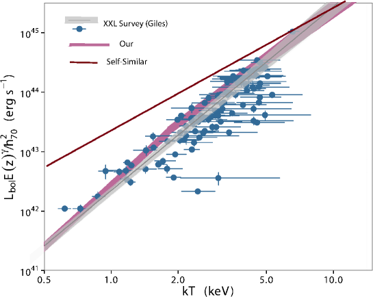
Figure 1: Comparison of the LTR from (Giles et al., 2016), represented by the dots with error-bars and the gray line, with our model. The plot shows the bolometric LTR, with data corrected for the bias. The black solid line is the best fitting model, and the gray band represents the 1 $\sigma$ uncertainty. The red band represents our result, while the brown line is the prediction of the self-similar model, $L\propto T^{2}$.

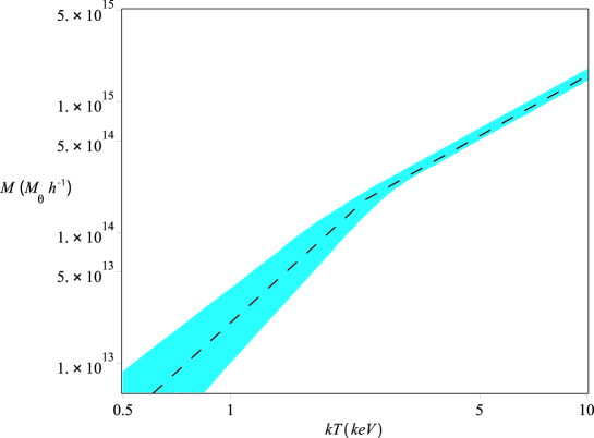
Figure 2: The MTR obtained with the model from Sec. II. The dashed line is the average value. The cyan region shows the 68% confidence level region, obtained according to (Afshordi and Cen, 2002), and (Del Popolo et al., 2019).

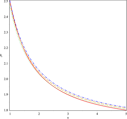
Figure 3: The collapse threshold $\delta_{c}(\nu)$ as a function of $\nu$. The red solid line shows the result from (Sheth et al., 2001, Eq. 4), the green short-dashed line the results of (Del Popolo and Gambera, 1998), taking into account the effect of the tidal field, the orange long-dashed the result of (Del Popolo, 2006a) taking into account the effect of the tidal field and the cosmological constant, while the blue dot-dashed line takes into account the effect of the tidal field, the cosmological constant and DF.

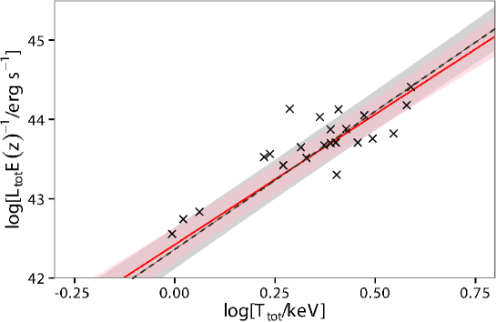
Figure 4: Bolometric LTR of 400d groups sample with bias-correction. The bias corrected model is represented by the red solid line, and the pink shaded region. The black dashed lines and the gray dashed region represents our result.

III An improved “punctuated equilibria model”

In this section, we extend the “punctuated equilibria model” (PEM) from (Cavaliere et al., 1997, 1998, 1999), taking into account the angular momentum acquisition from the proto-structure, and for the first time the DF.

In Cavaliere et al. (1998), the cluster evolution is described as a sequence of “punctuated equilibria” (PE). These are a sort of sequence of hierarchical merging episodes of the DM halos, related in the intra-cluster plasma (ICM) to shocks of various strengths providing the boundary conditions so that the ICM may re-adjust to a new hydrostatic equilibrium.

Following Balogh et al. (1999)’s notation, one can obtain the bolometric X-ray luminosity from Bremsstrahlung. If the cluster gas temperature is $T_{\color[rgb]{0,0,0}{g}}(r)$, its density profile $\rho_{\rm g}(r)$, we can write

$$L={6\pi k\over C_{1}(\mu m_{\rm p})^{2}}\int_{0}^{R_{\rm vir}}r^{2}\rho_{g}(r)^{2}T_{g}(r)^{1/2}dr$$ (14)

Balogh et al. (1999), where $\mu=0.59$, $C_{1}=3.88\times 10^{11}$s K^-1/2 cm^-3. Assuming that $\rho_{\rm g}\propto\rho$ one obtains the simplest model describing the L-T relation that can be calculated by Eq. (14), namely the self-similar-model of Kaiser (1986).

In Cavaliere et al. (1998)’s notation, Eq. (14), is written with a similar form

$$L\propto\int_{o}^{r_{2}}\,n^{2}(r)\,T^{1/2}(r)\,d^{3}r~{}.$$ (15)

Here $T(r)$ is the temperature in the plasma. A cluster boundary, $r_{2}$, is considered that is taken to be close to the virial radius $R_{\rm vir}\propto M_{\rm vir}^{1/3}\,\rho^{-1/3}$.

As shown in App. A, the luminosity-mass relation can be cast in the form:

$$L\propto \Big{(}{n_{2}\over n_{1}}\Big{)}^{2}\,\rho\,\Bigg{[}{T_{2}\over T_{v}}\Bigg{]}^{1/2}\,\overline{[n(r)/n_{2}\big{]}^{2+(\gamma-1)/2}}M^{4/3}$$

$$\sqrt{\frac{\frac{1}{m}+\left({\frac{t_{{\Omega}}}{t}}\right)^{2/3}+\frac{K}{\left({\frac{M}{M_{{0}}}}\right)^{8/3}}+\frac{\lambda_{0}}{1-\mu(\delta)}\frac{\Lambda\xi^{3}}{3H_{0}^{2}\Omega_{m},0}}{\frac{1}{m}+\left({\frac{t_{{\Omega}}}{t}}\right)^{2/3}+{\frac{K_{{0}}}{{M_{{0}}}^{8/3}}}}}{\color[rgb]{0,0,0}{.}}$$ (16)

See App. A for a derivation of Eq. (16) and a definition of the terms involved. From the luminosity-mass relation the LTR can be obtained using the relation between mass and temperature (see also Del Popolo et al., 2005).

We may now calculate the average value of $L$ and its dispersion, associated with a given cluster mass.

To this aim, we sum over the shocks produced at a time $t^{\prime}<t$ in all possible progenitors $M^{\prime}$ by the accreted clumps $\Delta M$; then, we integrate over time $t^{\prime}$ from an effective lower limit $t-\Delta t$. As found by Cavaliere et al. (1999) the average $L$ is given by

$$\langle L\rangle = Q\,\int_{t-\Delta t}^{t}\,dt^{\prime}\,\int_{0}^{m}\,dM^{\prime}\,\int_{0}^{M-M^{\prime}}\,d\Delta M\,$$

$$\frac{df}{dM^{\prime}}(M^{\prime},t^{\prime}|M,t)\,\frac{d^{2}p(M^{\prime}\rightarrow M^{\prime}+\Delta M)}{d\Delta M\,dt^{\prime}}\,L~{};$$

and the variance is given by

$$\langle\Delta L^{2}\rangle = Q\,\int_{t-\Delta t}^{t}\,dt^{\prime}\int_{0}^{M}\,dM^{\prime}\,\int_{0}^{M-M^{\prime}}\,d\Delta M\,$$ (18)

$$\,{df\over dM^{\prime}}(M^{\prime},t^{\prime}|M,t)\,{d^{2}p(M^{\prime}\rightarrow M^{\prime}+\Delta M)\over d\Delta M\,dt^{\prime}}$$

$$\Big{(}L-\langle L\rangle\Big{)}^{2}~{}.$$

where $Q$ is the normalisation factor .

The effective lower limit for the integration over masses is set as described in (Cavaliere et al., 1999, Sec. (2.4)).

IV Results and discussion

The results of the calculations are represented in Figs. 1-4. In Fig. 1 we plot the comparison with our present model of the LTR of (Giles et al., 2016) represented by the dots with error-bars, and the gray line. The plot shows the bolometric LTR. The data are corrected for the bias, the solid line is the best fitting model, and the gray band represents the 1 $\sigma$ uncertainty. The red band represents our result, while the brown line is the prediction of the self-similar model, $L\propto T^{2}$. As shown by the plot, our model is in agreement with the survey of (Giles et al., 2016), but in contrast with their best fit model, it shows a slight break at $\simeq 2$ keV. The upper line has a slope of $2.76\pm 0.18$, while the bottom one $3.4\pm 0.18$. The (Giles et al., 2016) bolometric LTR has a slope $3.08\pm 0.15$. The slopes are in agreement within the limits of errors. As discussed previously, the break, and the different slopes at high mass and low mass are in agreement with the prediction of some observations (Helsdon and Ponman, 2000; Sun et al., 2009). The same kind of break is observed in the MTR relation shown in Fig. 2 (see also Del Popolo et al., 2019). The MTR presents a non-self similar behavior with a break around 3 keV. At smaller masses the central slope of the MTR in the range $0.5-3$ keV is $\simeq 2.3$. Such bend has been observed by (Finoguenov et al., 2001), who explained it as due to the formation redshift. Similarly to the LTR, another possibility to explain the bend in the MTR relies on the preheating of the ICM in the early phase of formation (Xu et al., 2001). As noticed by (Giles et al., 2016) there is a dependence between the LTR and the MTR. The trends of one somehow are reflected in the other. As shown by the Fig. 1, both (Giles et al., 2016)’s result, and our’s show that the slope of the LTR is steeper than the self-similar case, $L\propto T^{2}$. They tend to appear closer to $L\propto T^{3}$. We have seen that this large steepness is due to different possible reasons, such as pre-heating, supernovae feedback, or outflows generated by AGN at high redshift that blows cavities, and AGN heating, raising the entropy of the ICM, thus reducing its density, and consequently the X-ray luminosity, by that removing the gas in a large area reaching the cluster virial radius. In other words, for some physical reasons, the core gas density is smaller than what is expected in the self-similar model. This can be understood more easily by taking the example of an episode of supernovae feedback heating the gas that could make it harder to compress in the core. Preheating or similar models then give rise to a steeper LTR because they change the density in the center of the cluster. As discussed in (Del Popolo et al., 2005), the same effect can be produced by angular momentum acquired by the cluster. As discussed in (Del Popolo and Gambera, 1998), angular momentum acquired by a shell of matter centered in a peak of the CDM density distribution is anti-correlated with density. Namely, high density peaks acquire less angular momentum than low-density peaks (Hoffman, 1986; Ryden, 1988). Larger amounts of angular momentum acquired by low-density peaks lead these peaks to resist more easily to gravitational collapse. In our model, we added the effect of DF, compared with (Del Popolo et al., 2005), and as shown, for example in (Del Popolo, 2009, App. D, and Fig. 11), DF amplifies the effects of angular momentum.

A more extended discussion of the reason why the LTR relation is steeper than the self-similar relation, $L\propto T^{2}$, follows.

In our model the breaking of self-similarity is due to tidal interactions between neighboring perturbations, the predecessor of the clusters. The interaction arises due to the asphericity of clusters, and to the effect of DF. The relation between the acquisition of angular momentum, asphericity, and structure formation was discussed in (Del Popolo and Gambera, 1999). Apart from the steepening from $L\propto T^{2}$ to $L\propto T^{\simeq 3}$, as shown in Figs. 1 and 2, a bend around a few keV can be found. That bend depends on the asphericity, and appears both in the LTR and in the MTR. Then, for clusters having $T<2\rm keV$, the luminosity is smaller than for clusters with higher energies. The difference with the self-similar solution increases going towards smaller masses. Our MTR, and LTR are characterized by a mass dependent angular momentum, $L$, that originates in the quadruple momentum of the proto-cluster. This is responsible of the breaking of self-similarity, to which we must add the effect of DF that behaves similarly to angular momentum, delaying the collapse of the cluster. In more details, the collapse in our model occurs in a different way than in the case of the simple spherical collapse model. In our model, the collapse threshold, $\delta_{c}$, and the time of collapse change. Differently from the simple spherical collapse, the threshold $\delta_{c}$ becomes mass dependent as shown in several papers [e.g., Del Popolo and Gambera 1999: Eq. 14, Fig. 1; Del Popolo 2006b: Fig. 5], and becomes a monotonic decreasing function of mass, as shown in Fig. 3 of the present paper. As the plot shows, $\delta_{c}$ is larger with respect to the standard value at the galactic mass scale, and moves to the standard value, going towards cluster mass scales. In Fig. 3, the red solid line shows the result from (Sheth et al., 2001, Eq. 4), the green short-dashed line, the results of (Del Popolo and Gambera, 1998) taking into account the effect of the tidal field, the orange long-dashed line, the result of (Del Popolo, 2006a) taking into account the effect of the tidal field and the cosmological constant, while the blue dot-dashed line takes into account the effect of the tidal field, the cosmological constant and DF. As can be seen from the plot, the effects of tidal torques, cosmological constant, and DF are additive, and tend to make $\delta_{c}$ increase.

Moreover there is a correlation between the temperature and threshold $\delta_{c}$: $T\propto\epsilon\propto\delta_{c}$ (see Voit, 2000). This means that less massive clusters are hotter than more massive ones, characterized by a standard MTR.

Another factor modifying the LTR, as well as the MTR, is the modification of energy partition in virial equilibrium (Del Popolo and Gambera, 1999). Another fundamental role is taken by the cosmological constant, and DF. The effect of these two quantities are also similar to that of angular momentum, namely that of delaying the collapse of the perturbation, and modifying $\delta_{c}$. A comparison of angular momentum, cosmological constant, and DF, represented by the three terms after the gravitational force in Eq. (1), is shown in Fig. 3. These quantities have a similar order of magnitude, with differences of order of a few percent. The effect of DF is calculated as in (Del Popolo, 2006b, 2009). There are several papers studying the role of DF in clusters formation (White, 1976; Kashlinsky, 1984, 1986, 1987). The effect of substructure was calculated by (Antonuccio-Delogu and Colafrancesco, 1994), who also showed that DF gives rise to a delay in the collapse of low height ($\nu$) peaks, with consequences similar to that of tidal torques. DF and tidal torques produce changes in several quantities like: the threshold of collapse $\delta_{c}$, the mass function, the temperature at a given mass, and the correlation function. DF has a similar effect on structure formation to that of tidal torques. It slows down the collapse, and as a consequence the density in the central region of the halo decreases.

We have seen that both the MTR and the LTR at some keV show a steepening, and that clusters with lower mass than the bend are hotter (less luminous) than expected. To further check the LTR at the low mass regime, we compared the results of our model with that of a study by (Zou et al., 2016), dealing with $Chandra$ observations of 23 galaxy groups and low-mass clusters of galaxies. The comparison of our results with the clusters from (Zou et al., 2016) is plotted in Fig. 4. The figure plots the bolometric LTR of the 400d groups sample with bias correction, as the red solid line with the pink shaded error region. The black dashed line and the gray dashed region represent our results. In (Zou et al., 2016), the LTR relation was studied, finding that its slope is more or less in agreement with that of large mass clusters, evaluated at $3.29\pm 0.33$. In our case we obtained $3.35\pm 0.3$. From a comparison with the clusters of the XXL survey of (Giles et al., 2016, $3.08\pm 0.15$), it is evident that the maximum slope is in this last case 3.23, while for the case of the (Zou et al., 2016) groups it reaches 3.62. In other terms, even if the groups, and clusters have similar behavior, groups seems to have a steeper slope in agreement with other studies (Helsdon and Ponman, 2000; Sun et al., 2009), and in agreement with our results.

Note that the X-ray luminosity, at energies close to 1 KeV, especially at the level of groups where the emission in the Fe-L band becomes very relevant, depends on the assumed metallicity Giles et al. (2016); Zou et al. (2016); Sun et al. (2009); Eckmiller et al. (2011); Maughan et al. (2012): the larger the metallicity, the larger $L_{X}$ is. In this paper we have employed the solar metallicity (0.3) from emission models such as APEC Smith et al. (2001) or XSPEC Arnaud (1996).

V Conclusions

In the present work, we obtained an LTR extending the results of a previous paper (Del Popolo et al., 2005), additionally taking into account in the model the effects of DF. Under the assumption of self-similarity (Kaiser, 1986), one can obtain a simple scaling law between the luminosity and temperature. The relation is of the type $L\propto T^{2}$. A large number of studies have shown that in reality the relation between luminosity and temperature is steeper, $L\propto T^{\simeq 3}$. There are several reason for this discrepancy between theory and observations. The difference is mainly due to energy input by non-gravitational processes, like pre-heating, supernovae feedback, and heating from AGN. In this paper, we studied the LTR by means of a modified version of the (Cavaliere et al., 1999) punctuated equilibria model, taking, in addition, DF into account, while it was ignored in (Del Popolo et al., 2005). We showed that the model is predicting a non-self-similar behavior of the LTR. The LTR features a bend at $\simeq 2$ keV, with a slope $2.76\pm 0.18$ for larger energies and $3.4\pm 0.18$ for energies smaller than 2 keV. This behavior is in agreement with the result of the XXL survey (Giles et al., 2016), shifting the slope to $3.08\pm 0.15$. The steeper slopes at smaller energies is in agreement with some studies (Helsdon and Ponman, 2000; Sun et al., 2009, e.g.) claiming a further steepening of the LTR at the low mass end. In order to check such slightly steeper LTR slope in small mass clusters and groups of galaxies, we used the study of (Zou et al., 2016) for the 400d groups sample, and compared our result with them. This study, in agreement with ours, indeed displays a slope $3.29\pm 0.33$, steeper than clusters of the XXL survey from (Giles et al., 2016, $3.08\pm 0.15$).

Appendix A L-T relation in the MPEM

As we saw in Sec. III that Eq. (14) gives the X-ray bolometric luminosity of a cluster. Using Cavaliere et al. (1998)’s notation the equation is written as

$$L\propto\int_{o}^{r_{2}}\,n^{2}(r)\,T^{1/2}(r)\,d^{3}r~{}.$$ (19)

$T(r)$ indicates the plasma temperature. The cluster has a boundary $r_{2}$ close to the virial radius $R_{\rm vir}\propto M^{1/3}\,\rho^{-1/3}$ and at this radius the gas is supersonic forming a shock front Takizawa and Mineshige (1998). Mass, and energy conservation is represented by the Rankine-Hugoniot conditions, describing the jumps in temperature and density from the outer region of the shock where temperature and density are $T_{1}$ and $n_{1}$ to $T_{2}$ and $n_{2}$ in the region interior to $r_{2}$. Then we may write the luminosity as

$$L\propto r_{2}^{3}\;n_{2}^{2}\,T_{2}^{1/2}\;\int_{0}^{1}d^{3}x\,\Big{[}{n(x)\over n_{2}}\Big{]}^{2}\,\Big{[}{T(x)\over T_{2}}\Big{]}^{1/2}~{},$$ (20)

where $x\equiv r/r_{2}$. $n_{1}$ is proportional to the universal baryonic fraction $f_{u}$, and average cosmic DM density $\rho_{u}$ at formation, taking the form $n_{1}\propto f_{u}\,\rho_{u}/m_{p}$. The inner temperature $T_{1}$ is obtained in a statistical way by means of the diverse merging histories ending up in the mass $M$. In summary, for each dark mass $M$ exists a set of equilibria states of the intra-cluster plasma (ICP) corresponding to different initial conditions. Each one of these equilibria states correspond to a different realization of the merging history. The average values of luminosity, $L$, and $R_{X}$, and their scatter are obtained from the convolution over such set. According to Cavaliere et al. (1998), in a merging event the temperature before the shock, during a merging, is considered equal to that of the infalling gas. If the latter is inside a deep potential well, $T_{1}$ is the virial temperature $T_{1v}\propto\Delta M/r$ of the partner in secondary merging. If $r\propto(\Delta M/\rho)^{1/3}$, the virial temperature fulfills the relation

$$k\,T_{1v}=4.5\,(\Delta M)^{2/3}\,(\rho/\rho_{o})^{1/3}~{}{\rm keV},$$ (21)

where the masses $M/M_{0}$ are normalised to the mass inside a sphere of $8h^{-1}$ Mpc, giving the current value $M_{0}=0.6\times 10^{15}\Omega_{0}h^{-1}M_{\odot}$, and the numerical factor comes from Hjorth et al. (1998).

Preheating of diffuse external gas, generated by feedback energy inputs (e.g., supernovae) gives rise to a lower bound $kT_{1*}\approx 0.5$ keV Renzini (1997).

Then the actual value of $T_{1}$ is

$$T_{1}=max\,\big{[}T_{1v},T_{1*}\big{]}$$ (22)

Given the $T_{1}$ value, the boundary conditions for the ICP is given by the shocks strength. The value of $T_{2}$ in the case of a nearly hydrostatic post-shock condition with $v_{2}<<v_{1}$, three degrees of freedom, and the velocity of the shock that matches the growth rate of the virial radius, follows

$$kT_{2}={{\mu m_{p}v_{1}^{2}}\over 3}\Big{[}{{(1+\sqrt{1+\epsilon})^{2}}\over 4}+{7\over{10}}\epsilon-{{3}\over{20}}{{\epsilon^{2}}\over{(1+\sqrt{1+\epsilon})^{2}}}\Big{]}\,.$$ (23)

Cavaliere et al. (1997), where $\epsilon\equiv 15kT_{1}/4\mu m_{p}v_{1}^{2}$ and $\mu$ is the average molecular weight. $v_{1}$, namely the inflow velocity is fixed by the potential drop across the region of free fall, and is given by $v_{1}\simeq\sqrt{-\phi_{2}/m_{p}}$, being $\phi_{2}$ the potential at $r_{2}$. For strong shocks (“cold inflow”) $\epsilon<<1$. The approximation

$$kT_{2}\simeq-\phi_{2}/3+3kT_{1}/2$$ (24)

holds in the case of rich clusters accreting diffuse gas in small clumps. Here, $\phi_{2}$ represents the gravitational potential energy at $r_{2}\simeq R_{\rm vir}$. In the case of weak shocks ($\epsilon\geq 1$), we have that $T_{2}\simeq T_{1}$. Following Cavaliere et al. (1997), the density jump is given by

$${n_{2}\over n_{1}}=2\,\Big{(}1-{T_{1}\over T_{2}}\Big{)}+\Big{[}4\,\Big{(}1-{T_{1}\over T_{2}}\Big{)}^{2}+{T_{1}\over T_{2}}\Big{]}^{1/2}~{}.$$ (25)

With the polytropic temperature description $T(x)/T_{2}=[n(x)/n_{2}]^{\gamma-1}$, where $1\leq\gamma\leq 5/3$, and assuming that $r_{2}$ may be related to it, written as $T_{\rm v}\propto M/r_{2}$ and that $M\propto\rho r_{2}^{3}$, (leading to $r_{2}\propto(t/\rho)^{1/2}$), we get the luminosity in the form

$$L\propto\Big{(}{n_{2}\over n_{1}}\Big{)}^{2}\,MT_{v}^{1/2}\,\rho\,\Bigg{[}{T_{2}\over T_{v}}\Bigg{]}^{1/2}\,\overline{[n(r)/n_{2}\big{]}^{2+(\gamma-1)/2}}~{}.$$ (26)

The bar in the previous expression represents the integration over the emitting volume $r^{3}\leq r_{2}^{3}$, while $\rho$ (proportional to $\rho_{u}$ and so to $n_{1}$) is the average DM density in the cluster.

Eq. (26) can also be cast in the form:

$$L \propto \Big{(}{n_{2}\over n_{1}}\Big{)}^{2}\,\rho\,\Bigg{[}{T_{2}\over T_{v}}\Bigg{]}^{1/2}\,\overline{[n(r)/n_{2}\big{]}^{2+(\gamma-1)/2}}M^{4/3}$$ (27)

$$\sqrt{\frac{\frac{1}{m}+\left({\frac{t_{{\Omega}}}{t}}\right)^{2/3}+\frac{K}{\left({\frac{M}{M_{{0}}}}\right)^{8/3}}+\frac{\lambda_{0}}{1-\mu(\delta)}\frac{\Lambda\xi^{3}}{3H_{0}^{2}\Omega_{m},0}}{\frac{1}{m}+\left({\frac{t_{{\Omega}}}{t}}\right)^{2/3}+{\frac{K_{{0}}}{{M_{{0}}}^{8/3}}}}}$$

where $\lambda_{0}=\epsilon_{0}T_{\rm c0}$, $\mu(\delta)$, $\xi$, $M$, $t_{\Omega}$, and the function $K$ are given in Sec. II of the present paper.

Using the hydrostatic equilibrium, $dP/m_{p}\,n\,dr=-G\,M(<r)/r^{2}=-d\phi/dr$, together with the polytropic pressure $P(r)=kT_{2}\,n_{2}\,\big{[}{n(r)/n_{2}}\big{]}^{\gamma}$, we obtained the ratio $n(x)/n_{2}$. This gives rise to the profiles

$${n(r)\over n_{2}}=\Big{[}{T(r)\over T_{2}}\Big{]}^{1/(\gamma-1)}=\Big{\{}1+{\gamma-1\over\gamma}\,\beta\,\big{[}\tilde{\phi}_{2}-\tilde{\phi}(r)\big{]}\Big{\}}^{1/(\gamma-1)}~{},$$ (28)

being $\tilde{\phi}\equiv\phi/\mu\,m_{p}\,\sigma_{2}^{2}$ the potential normalised to the relative one-dimensional DM velocity dispersion at the radius $r_{2}$. The parameter $\beta$ is given by

$$\beta=\mu m_{p}\sigma_{2}/kT_{2}~{}.$$ (29)

Eq. (24) for a given DM potential $\phi_{2}$ allows to obtain the function $\beta(T)$ corresponding to $\rho(r)$, and $\phi(r)$, while $\sigma(r)$ can be obtained by means of Navarro-Frenk-White profile (Navarro et al., 1997). $\beta(T)$ goes from $\beta\simeq 0.5$ for $T\simeq T_{1}$ to $\beta\simeq 0.9$ for $T>>T_{1}$. Following (Cavaliere et al., 1999), and the observations of Markevitch et al. (1998) $\gamma=1.2\pm 0.1$. We will use the value $\gamma=1.2$ in the calculation.

References

- Del Popolo et al. (2005) A. Del Popolo, N. Hiotelis, and J. Peñarrubia, ApJ 628, 76 (2005), arXiv:astro-ph/0508596 [astro-ph] .
- Cavaliere et al. (1999) A. Cavaliere, N. Menci, and P. Tozzi, MNRAS 308, 599 (1999), arXiv:astro-ph/9810498 [astro-ph] .
- Giles et al. (2016) P. A. Giles et al., Astron. Astrophys. 592, A3 (2016), arXiv:1512.03833 [astro-ph.CO] .
- Zou et al. (2016) S. Zou, B. J. Maughan, P. A. Giles, A. Vikhlinin, F. Pacaud, R. Burenin, and A. Hornstrup, MNRAS 463, 820 (2016), arXiv:1610.07674 [astro-ph.CO] .
- Clowe et al. (2006) D. Clowe, M. Bradač, A. H. Gonzalez, M. Markevitch, S. W. Randall, C. Jones, and D. Zaritsky, ApJL 648, L109 (2006), arXiv:astro-ph/0608407 [astro-ph] .
- Markevitch et al. (1998) M. Markevitch, W. R. Forman, C. L. Sarazin, and A. Vikhlinin, ApJ 503, 77 (1998), arXiv:astro-ph/9711289 [astro-ph] .
- Horner et al. (1999) D. J. Horner, R. F. Mushotzky, and C. A. Scharf, ApJ 520, 78 (1999), astro-ph/9902151 .
- Maughan (2007) B. J. Maughan, ApJ 668, 772 (2007), arXiv:astro-ph/0703504 [astro-ph] .
- Kaiser (1986) N. Kaiser, MNRAS 222, 323 (1986).
- Bower (1997) R. G. Bower, MNRAS 288, 355 (1997), arXiv:astro-ph/9701014 [astro-ph] .
- Mushotzky (1984) R. F. Mushotzky, Physica Scripta Volume T 7, 157 (1984).
- Ettori et al. (2004) S. Ettori, P. Tozzi, S. Borgani, and P. Rosati, A&A 417, 13 (2004), arXiv:astro-ph/0312239 [astro-ph] .
- Mittal et al. (2011) R. Mittal, A. Hicks, T. H. Reiprich, and V. Jaritz, A&A 532, A133 (2011), arXiv:1106.5185 [astro-ph.CO] .
- Maughan et al. (2012) B. J. Maughan, P. A. Giles, S. W. Randall, C. Jones, and W. R. Forman, MNRAS 421, 1583 (2012), arXiv:1108.1200 [astro-ph.CO] .
- Pratt et al. (2009) G. W. Pratt, J. H. Croston, M. Arnaud, and H. Böhringer, A&A 498, 361 (2009), arXiv:0809.3784 [astro-ph] .
- Connor et al. (2014) T. Connor, M. Donahue, M. Sun, H. Hoekstra, A. Mahdavi, C. J. Conselice, and B. McNamara, ApJ 794, 48 (2014), arXiv:1409.1590 [astro-ph.CO] .
- Osmond and Ponman (2004) J. P. F. Osmond and T. J. Ponman, MNRAS 350, 1511 (2004), arXiv:astro-ph/0402439 [astro-ph] .
- Helsdon and Ponman (2000) S. F. Helsdon and T. J. Ponman, MNRAS 315, 356 (2000), arXiv:astro-ph/0002051 [astro-ph] .
- Sun et al. (2009) M. Sun, G. M. Voit, M. Donahue, C. Jones, W. Forman, and A. Vikhlinin, ApJ 693, 1142 (2009), arXiv:0805.2320 [astro-ph] .
- Lovisari et al. (2015) L. Lovisari, T. H. Reiprich, and G. Schellenberger, A&A 573, A118 (2015), arXiv:1409.3845 [astro-ph.CO] .
- Del Popolo (2002) A. Del Popolo, MNRAS 336, 81 (2002), arXiv:astro-ph/0205449 [astro-ph] .
- Voit and Donahue (1998) G. M. Voit and M. Donahue, ApJL 500, L111 (1998), astro-ph/9804306 .
- Voit (2000) G. M. Voit, ApJ 543, 113 (2000), astro-ph/0006366 .
- Afshordi and Cen (2002) N. Afshordi and R. Cen, ApJ 564, 669 (2002), astro-ph/0105020 .
- Del Popolo et al. (2019) A. Del Popolo, F. Pace, and D. F. Mota, Phys. Rev. D 100, 024013 (2019), arXiv:1908.07322 [astro-ph.CO] .
- Lacey and Cole (1993) C. Lacey and S. Cole, MNRAS 262, 627 (1993).
- Del Popolo (2009) A. Del Popolo, ApJ 698, 2093 (2009), arXiv:0906.4447 [astro-ph.CO] .
- Peebles (1993) P. J. E. Peebles, Princeton Series in Physics, Princeton, NJ: Princeton University Press, —c1993, edited by P. J. E. Peebles (1993).
- Bartlett and Silk (1993) J. G. Bartlett and J. Silk, ApJL 407, L45 (1993).
- Lahav et al. (1991) O. Lahav, P. B. Lilje, J. R. Primack, and M. J. Rees, MNRAS 251, 128 (1991).
- Del Popolo and Gambera (1998) A. Del Popolo and M. Gambera, A&A 337, 96 (1998), astro-ph/9802214 .
- Del Popolo and Gambera (1999) A. Del Popolo and M. Gambera, A&A 344, 17 (1999), arXiv:astro-ph/9806044 .
- Antonuccio-Delogu and Colafrancesco (1994) V. Antonuccio-Delogu and S. Colafrancesco, ApJ 427, 72 (1994).
- Sheth et al. (2001) R. K. Sheth, H. J. Mo, and G. Tormen, MNRAS 323, 1 (2001), arXiv:astro-ph/9907024 .
- Del Popolo (2006a) A. Del Popolo, ApJ 637, 12 (2006a), astro-ph/0609100 .
- Cavaliere et al. (1997) A. Cavaliere, N. Menci, and P. Tozzi, ApJL 484, L21 (1997), arXiv:astro-ph/9705058 [astro-ph] .
- Cavaliere et al. (1998) A. Cavaliere, N. Menci, and P. Tozzi, ApJ 501, 493 (1998), arXiv:astro-ph/9802185 [astro-ph] .
- Balogh et al. (1999) M. L. Balogh, A. Babul, and D. R. Patton, MNRAS 307, 463 (1999), arXiv:astro-ph/9809159 [astro-ph] .
- Finoguenov et al. (2001) A. Finoguenov, T. H. Reiprich, and H. Böhringer, A&A 368, 749 (2001), arXiv:astro-ph/0010190 .
- Xu et al. (2001) H. Xu, G. Jin, and X.-P. Wu, ApJ 553, 78 (2001), astro-ph/0101564 .
- Hoffman (1986) Y. Hoffman, ApJ 301, 65 (1986).
- Ryden (1988) B. S. Ryden, ApJ 329, 589 (1988).
- Del Popolo (2006b) A. Del Popolo, A&A 454, 17 (2006b), arXiv:0801.1086 .
- White (1976) S. D. M. White, MNRAS 174, 19 (1976).
- Kashlinsky (1984) A. Kashlinsky, MNRAS 208, 623 (1984).
- Kashlinsky (1986) A. Kashlinsky, ApJ 306, 374 (1986).
- Kashlinsky (1987) A. Kashlinsky, ApJ 312, 497 (1987).
- Eckmiller et al. (2011) H. J. Eckmiller, D. S. Hudson, and T. H. Reiprich, Astron. Astrophys. 535, A105 (2011), arXiv:1109.6498 [astro-ph.CO] .
- Smith et al. (2001) R. K. Smith, N. S. Brickhouse, D. A. Liedahl, and J. C. Raymond, Astrophys. J. Lett. 556, L91 (2001), arXiv:astro-ph/0106478 .
- Arnaud (1996) K. A. Arnaud, in Astronomical Data Analysis Software and Systems V, Astronomical Society of the Pacific Conference Series, Vol. 101, edited by G. H. Jacoby and J. Barnes (1996) p. 17.
- Takizawa and Mineshige (1998) M. Takizawa and S. Mineshige, ApJ 499, 82 (1998), arXiv:astro-ph/9702047 [astro-ph] .
- Hjorth et al. (1998) J. Hjorth, J. Oukbir, and E. van Kampen, MNRAS 298, L1 (1998), arXiv:astro-ph/9802293 [astro-ph] .
- Renzini (1997) A. Renzini, ApJ 488, 35 (1997), arXiv:astro-ph/9706083 [astro-ph] .
- Navarro et al. (1997) J. F. Navarro, C. S. Frenk, and S. D. M. White, ApJ 490, 493 (1997), astro-ph/9611107 .