Reinforcement Learning with Tensor Networks: Application to Dynamical Large Deviations

Abstract

We present a framework to integrate tensor network (TN) methods with reinforcement learning (RL) for solving dynamical optimisation tasks. We consider the RL actor-critic method, a model-free approach for solving RL problems, and introduce TNs as the approximators for its policy and value functions. Our “actor-critic with tensor networks” (ACTeN) method is especially well suited to problems with large and factorisable state and action spaces. As an illustration of the applicability of ACTeN we solve the exponentially hard task of sampling rare trajectories in two paradigmatic stochastic models, the East model of glasses and the asymmetric simple exclusion process (ASEP), the latter being particularly challenging to other methods due to the absence of detailed balance. With substantial potential for further integration with the vast array of existing RL methods, the approach introduced here is promising both for applications in physics and to multi-agent RL problems more generally.

Introduction. Tensor networks, routinely used in the study of quantum many-body systems White (1992, 1993); Schollwöck (2011); Eisert et al. (2010); Eisert (2013); Montangero (2018); Orús (2019), have in recent years seen increasing application in the field of machine learning (ML) Stoudenmire and Schwab (2016); Liu et al. (2018); Sun et al. (2019); Roberts et al. (2019); Ghahramani and Jordan (1997); Efthymiou et al. (2019); Stoudenmire (2018); Han et al. (2018); Gao et al. (2019); Levine et al. (2019); Guo et al. (2018); Glasser et al. (2018, 2019). Both domains typically deal with systems that have state-spaces which are exponentially large in the number of degrees of freedom, be it the number of qubits in a quantum system, or the number of pixels in an image to be classified in an ML task. In such situations, tensor networks (TNs) provide a powerful method for representing functions, vectors and distributions, while allowing for efficient sampling and computation of quantities such as inner products and norms.

To date, the intersection of TNs and ML has been mostly in the areas of supervised and unsupervised learning Stoudenmire and Schwab (2016); Liu et al. (2018); Sun et al. (2019); Roberts et al. (2019); Ghahramani and Jordan (1997); Efthymiou et al. (2019); Stoudenmire (2018); Han et al. (2018); Gao et al. (2019); Levine et al. (2019); Guo et al. (2018); Glasser et al. (2018, 2019). In comparison, the combination of TNs and reinforcement learning (RL) Sutton and Barto (2018) is more limited, despite the fact that RL has seen spectacular recent advances Mnih et al. (2015); Haarnoja et al. (2018); Silver et al. (2016); Schulman et al. (2015); Wang et al. (2019) much like the other two branches of ML. While some promising related directions have been explored, such as the approximation of Q-functions in the context of large state-spaces Metz and Bukov (2022), and/or large action-spaces Mahajan et al. (2021), a need for flexible integration of TNs with RL, along with a demonstration of useful application, has remained an open problem.

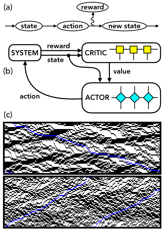
Figure 1: ACTeN (a) Markov decision process. (b) In actor-critic RL, the state is passed to an actor, which chooses the action, and to a critic, which values the state given the reward. This value is used to improve the actor’s policy. In ACTeN, the function approximators for actor and critic are tensor networks. (c) Top: typical ($\lambda=0$) trajectory of the ASEP at half-filling, with one particle highlighted (blue) ($L=50,T=3000,p=0.1$). Bottom: trajectory with a large current fluctuation ($\lambda=-3$), sampled from the ACTeN solution. Time and space are the $x$ and $y$ axis, respectively.

In this paper, we introduce the actor-critic with tensor networks (or ACTeN) method, a general framework for integrating TNs into RL via actor-critic techniques. Due to its model-free nature and the use of function approximation for both policy and value functions, actor-critic is a highly flexible approach, and many of the state-of-the-art applications of RL in a wide range of contexts have been achieved with it. Given the proven effectiveness of TNs to deal with systems with large number of degrees of freedom, using TNs as function appoximators within actor-critic RL represents an ideal combination to tackle problems with both large state and action spaces in a relatively straightforward manner.

To demonstrate the power of our approach, we consider the problem of computing the large deviation (LD) statistics of dynamical observables in classical stochastic systems Garrahan (2016, 2018); Jack and Sollich (2015); Jack (2019); Chetrite and Touchette (2015a); Casert et al. (2021), and of optimally sampling the associated rare long-time trajectories Majumdar and Orland (2015); Chetrite and Touchette (2015b); Bolhuis et al. (2002); Giardinà et al. (2006); Giardina et al. (2011); Cérou and Guyader (2007); Lecomte and Tailleur (2007); Whitelam et al. (2020); De Bruyne et al. (2021); Bruyne et al. (2021a, b); De Bruyne et al. (2022); Pozzoli and Bruyne (2022). Such problems are of wide interest in statistical mechanics and condensed-matter physics, and can be phrased straightforwardly as an optimization problem which may be solved with RL Rose et al. (2021); Das and Limmer (2019); Das et al. (2021, 2022) and other techniques Borkar et al. (2003); Ferré and Touchette (2018); Yan et al. (2022); Yan and Rotskoff (2022); Nemoto and Sasa (2014); Nemoto et al. (2017); Kappen and Ruiz (2016); Bolhuis et al. (2022); Holdijk et al. (2022). For concreteness we consider two models: (i) the East model, a kinetically constrained model used to study slow glassy dynamics, and (ii) the asymmetric exclusion process (ASEP), a paradigmatic model of non-equilibrium. We consider both models in one dimension with periodic boundaries (PBs) and single spin-flip discrete Markov dynamics. While the East model obeys detailed balance and can therefore be mapped to a Hermitian problem, the ASEP does not, evading straightforward use of TNs to compute spectral properties of the relevant dynamical generator. In contrast, we demonstrate below how the ACTeN framework can be applied to both problems irrespective of the equilibrium/non-equilibrium distinction, by computing their dynamical LDs for sizes well beyond those achievable with exact methods. Given the vast array of options for improving both model and algorithm, our results indicate that the overall framework outlined here is highly promising for applications more generally.

Reinforcement learning and actor-critic. A discrete-time Markov decision process (MDP) Sutton and Barto (2018), at each time $t\in[0,T]$, consists of stochastic variables $X_{t}=\left(S_{t},a_{t},R_{t}\right)$, for the state, action and reward, respectively, which we assume are drawn from $t$-independent finite sets, $\mathcal{S},\mathcal{A}$ and $\mathcal{R}$. Trajectories take the form $(X_{0},X_{1},...,X_{T})=\{X_{t}\}_{t=0}^{T}$ and are generated by a Markovian dynamics with probabilities $\prod_{t=1}^{T}P(X_{t}|X_{t-1})P(X_{0})$, where $P(X_{0})$ is some initial distribution.

Figure 1(a) sketches the sequence of steps in an MDP. We decompose the state dynamics, $P(S^{\prime}|S)=\sum_{a\in\mathcal{A}(S)}P(S^{\prime}|S,a)\pi(a|S)$, into the environment, $P(S^{\prime}|S,a)$, and the policy, $\pi(a|S)$, where $\mathcal{A}(S)$ is the set of possible actions from a state $S$. That is, given a state $S$, a possible action $a$ is chosen from the policy, and that action determines the possible transitions into a new state $S^{\prime}$, with $(S,a,S^{\prime})$ determining the reward $R_{t}$. In the typical scenario of policy optimisation, the policy is considered controllable and known, while the environment is given.

For concreteness, below we focus on MDPs that are “continuing”, and admit a steady state distribution, $\mu(S)$, that is independent of $X_{0}$. We can then define the average reward per time-step when following a given policy as $r(\pi)=\lim_{t\to\infty}\mathds{E}_{\pi}[R_{t}]$, where $\mathds{E}_{\pi}\left[\cdot\right]$ indicates a stationary state expectation over states and an expectation over transitions from those states generated by following a dynamics defined by policy $\pi$. The task of policy optimisation is thus to determine the policy $\pi^{*}$ that maximises $r(\pi)$.

RL refers to the group of methods that aim to discover optimal policies by using the experience gained from sampling trajectories of an MDP. In policy gradient methods, of which AC is an example, the policy (or “actor”) is approximated directly as $\pi_{w}(a|S)$ with parameters $w$, and optimized using the gradient of $r(\pi_{w})$ with respect to $w$. This can be expressed as an expected value over trajectories obtained by sampling the policy Sutton and Barto (2018),

$$\nabla_{w}r(\pi) =\mathds{E}\left[G_{t}\nabla_{w}\ln\pi_{w}(a_{t}|S_{t})\right]~{},$$ (1)

where $G_{t}=\sum_{\tau=t}^{\infty}\left[R_{\tau}-r(\pi)\right]$ are differential returns following $S_{t}$ sampled from the stationary state of $\pi_{w}(a|S)$. Actor-critic (AC) methods, see Fig. 1(b), approach this by optimising an auxillary approximation $v_{\psi}(S)$ with parameters $\psi$ for a value-function (or “critic”). The true value function $v_{\pi}$ this approximation targets is defined as satisfying the differential Bellman equation, $v_{\pi}(s)=\mathds{E}_{\pi}\left[v_{\pi}(S_{t+1})+R_{t}-r(\pi)|S_{t}=s\right]$. The $G_{t}$ in Eq. (1) is then replaced by the one-step temporal-difference (TD) error, $\delta=v_{\psi}(S_{t+1})+R_{t+1}-r(\pi_{w})-v_{\psi}(S_{t})$. This consists of the one-step approximation of the expected differential return, $\mathds{E}[G_{t}|S_{t+1}=s^{\prime}]\approx v_{\psi}(s^{\prime})+R_{t+1}-r(\pi_{w})$, minus a baseline, $v_{\psi}(S_{t})$.

Actor-critic with tensor networks (ACTeN). A tensor network is comprised of a set of tensors, $\{T_{i_{1}j_{1}k_{1}\cdots}^{[1]},T_{i_{2}j_{2}k_{2}\cdots}^{[2]},...\}$ contracted together in a given pattern, usually defined via a graph. The result of this contraction defines a multi-variable function, $\varphi(x)$, where $x$ represents a set of variables that select values for the free indices in the network. With this view, TNs can be integrated into AC by including them in the definitions of $\pi_{w}$ and $v_{\psi}$, cf. Fig. 1(b). We will refer to this general approach as actor-critic with tensor networks (ACTeN), combining TN architectures with more standard RL ones.

For concreteness, the form of ACTeN that we apply here is specialised to one-dimensional systems with PBs, choosing a matrix product state (MPS) and a matrix product operator (MPO) as TNs. These define functions $\varphi(x)$ and $\varphi(y,z)$, respectively, which can be expressed as

$$\varphi(x) =\operatorname{\operatorname{Tr}}\left[A_{x_{1}}A_{x_{2}}...A_{x_{N}}\right]~{}$$ (2)

and

$$\varphi(y,z) =\operatorname{\operatorname{Tr}}\left[A_{y_{1}z_{1}}A_{y_{2}z_{2}}...A_{y_{N}z_{N}}\right]~{}.$$ (3)

Here, $x=(x_{1},x_{2},...x_{N})$ means that the MPS defines a function of $N$ variables, which are assumed to be discrete, and $A_{x_{i}}$ and $A_{y_{i}z_{i}}$ are matrices (we will consider real valued only). Note that for $N_{x}^{[i]}$ possible values of $x_{i}$ there are $N_{x}^{[i]}$ possible matrices $A_{x_{i}}$, and similarly $N_{y}^{[i]}\times N_{z}^{[i]}$ possible matrices $A_{y_{i}z_{i}}$: the choice of $x,y,z$ fixes which of these are selected for inclusion in the matrix multiplications in Eqs. (2,3). For the MPS Eq. (2), the set of $N_{x}^{[i]}$ matrices with label $i$ constitutes an order-$3$ tensor with shape $\left(N_{x}^{[i]},\chi_{L}^{[i]},\chi_{R}^{[i]}\right)$ where $\chi_{L}^{[i]}$ and $\chi_{R}^{[i]}$ are termed the left and right “bond-dimensions”. Thus, the MPS represents a tensor network of $N$ tensors, each of order-$3$ with a total of $N$ free indices and $2N$ virtual indices. Throughout we will assume $\chi_{L}=\chi_{R}=\chi$, and translation invariance, so that the MPS is defined by a single tensor of shape $(N_{x},\chi,\chi)$. The MPO Eq. (3) is constructed similarly and defined by a tensor of order-$4$ with shape $(N_{y},N_{z},\chi,\chi)$.

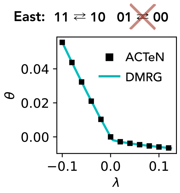
Figure 2: East Model Activity The east model is a canonical model of spin system dynamics subject to the kinetic constraint of facilitated excitation to the right, as depicted here. Due to detailed balance, the SCGF for the activity in the east model can be solved to high precision for large systems with DMRG. We find good agreement between the DMRG result and ACTeN up to $L=50$ across a range of biases.

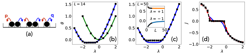
Figure 3: ASEP Current (a) The ASEP is another canonical spin model of dynamics subject to kinetic constraints. (b) The current in the ASEP cannot be tackled with DMRG, and exact comparisons are limited to small system sizes. Here, we find excellent agreement between ACTeN and the exact diagonalisation for $L=14$ for both $p=0.5$ (the SSEP, red line) and $p=0.1$ (blue line). (c) Going beyond exact diagonalisation to $L=50$, ACTeN again shows good results, with smooth convergence in $L$ (inset) and a clear flattening of the negative bias region (contrasted with the exact $L=14$) indicative of a phase transition. (d) Since ACTeN provides direct access to the optimal dynamics, observables such as the current can be evaluated directly (black squares). Here, this is compared with the exact result for $L=14$ (solid blue line) and the result of numerically differentiating the SCGF with $L=50$ (red circles).

To relate these TNs to RL, consider now $N$ agents, each associated to a single “site”, labelled by an integer $i=1,2,...,N$. Each agent has its own set of possible actions, $a_{i}$, drawn from the corresponding “local” action space, $a_{i}\in\mathcal{A}_{i}$. Additionally, each agent receives a (local) observation/state, $s_{i}\in\mathcal{S}_{i}$. The overall (“global”) action of the multi-agent system is given by $a=(a_{1},a_{2},...,a_{N})$, while the overall state is $S=(s_{1},s_{2},...,s_{N})$. For simplicity, we will assume that all $\mathcal{A}_{i}$ and $\mathcal{S}_{i}$ have the same size $N_{A}=|\mathcal{A}_{i}|$, $N_{S}=|\mathcal{S}_{i}|~{}\forall i$.

In this scenario, $v_{\psi}(S)$ is a function of $N$ variables, while $\pi_{w}(a|S)$ is a function of $2N$ variables and the total number of actions and states rise exponentially in the number of sites $N$. This precludes the use of direct (tabular) methods for all but the smallest systems. However, a definition of $v_{\psi}$ that is efficient to evaluate can be constructed using Eq. (2)

$$v_{\psi}(S) =\log\left[\varphi(s_{1},s_{2},...,s_{N})^{2}\right]~{}.$$ (4)

The parameters (“weights”) of this function approximation are denoted as $\psi$, and are contained in a single order-$3$ tensor of shape $(N_{S},\chi,\chi)$ that defines the translation invariant MPS, see Fig. 1(b).

To similarly define $\pi_{w}(a|S)$ while allowing for efficient sampling despite the large action space, we can use Eq. (3) and set $y_{i}=a_{i}$, $z_{i}=s_{i}$. A properly constrained policy can, e.g., be constructed as,

$$\pi_{w}(a|S)=\mathcal{C}(a,S)\frac{\varphi(a,S)^{2}}{\mathcal{N}(S)}~{},$$ (5)

where $\mathcal{N}(s)=\sum_{a|\mathcal{C}(a,S)=1}\varphi(a,S)^{2}$ is the (state-dependent) normalisation factor and $\mathcal{C}(a,S)$ returns one if an action $a$ is possible given a state $S$ or zero otherwise . The weights $w$ for this function approximation are contained in a single order-$4$ tensor of shape $(N_{A},N_{S},\chi,\chi)$, see Fig. 1(b).

With these definitions for $\pi_{w}$ and $v_{\psi}$, for practical implementation of ACTeN it remains to specify efficient computations (forward-passes) from a given $S$ SM . The computation of the gradients (backward-passes) can be then implemented easily using auto-differentiation methods available in standard ML frameworks (such as JAX Bradbury et al. (2018), which is the framework chosen here). Finally, a number of RL algorithms can be applied to optimise $\pi_{w}$. Here for simplicity we use a basic, single-step AC, with transitions sampled sequentially from a single long trajectory and updates performed according to standard gradient ascent SM . However, a wide variety of more sophisticated RL methods could allow for improvements in stability, efficiency and precision.

Application to dynamical large deviations and optimal sampling. To test ACTeN we consider the problem of computing the LDs of trajectory observables in the East model and the ASEP in 1D with PBs. Both models have states $S=(s_{1},s_{2},...,s_{L})$ where $s_{k}\in\{0,1\}$ indicate the occupations on lattice sites. Given a stochastic trajectory $\omega_{0}^{T}$ between times $0$ and $T$, the observables we consider, $O(\omega_{0}^{T})$, are the sum over time of quantities that depend solely on the current and prior states, $O(\omega_{0}^{T})=\sum_{t=1}^{T}o(S_{t},S_{t-1})$. As is standard in dynamical LDs, we are interested in computing the moment generating function (MGF) $Z_{T}(\lambda)=\sum_{\omega_{0}^{T}}e^{-\lambda O(\omega_{0}^{T})}$. The long-time limit is that of LDs, and the scaled cumulant generating function (SCGF), $\theta(\lambda)=\lim_{T\to\infty}\frac{1}{T}\ln Z_{T}(\lambda)$, plays the role of a dynamical free-energy density.

The SCGF can in principle be obtained by sampling an ensemble of trajectories reweighted by $e^{-\lambda O(\omega_{0}^{T})}$, but this is exponentially hard (in time and space) to do from the original dynamics. For $T\to\infty$, the optimal sampling dynamics can be defined variationally as the one that maximises the expected reward per time-step,

$$R_{t}=-\lambda o(S_{t},S_{t-1})-\ln\left(\frac{P_{w}\left(S_{t}|S_{t-1}\right)}{P_{\rm orig}\left(S_{t}|S_{t-1}\right)}\right).$$ (6)

Here, $P_{\rm orig}\left(S_{t}|S_{t-1}\right)$ is the original state-dynamics for the system while $P_{w}\left(S_{t}|S_{t-1}\right)$ is the (parameterised) dynamics to be optimised. At the optimal point, the expected reward per time-step is equal to the the SCGF $\theta(\lambda)$.

The connection to a MDP is as follows. The state $S$ of the MDP at time $t$ is the state of the lattice at that time. The action $a$ of the multi-agent is $a=(a_{1},a_{2},...,a_{N})$, where $a_{i}=1$ means flip site $i$ and $a_{i}=0$ means do nothing. The new state is then $S^{\prime}=f(a,s)=\{(1-a_{i})s_{i}+a_{i}(1-s_{i})\}_{i=1}^{L}$. To restrict actions to a single spin-flip per time step, we define the constraint function, $\mathcal{C}(a,S)$ in $\pi_{w}$ [cf. Eq. (5)], such that $\mathcal{C}(a,S)=1$ if $\sum_{i}a_{i}\leq 1$ or $\mathcal{C}(a,S)=0$ otherwise SM . We can then write $P_{w}(S^{\prime}|S)=\sum_{a}P(S^{\prime}|S,a)\pi_{w}(a|S)$. Furthermore, for a deterministic environment, $P(S^{\prime}|S,a)=\delta_{S^{\prime},f(a,S)}$. Therefore, $P_{w}(S^{\prime}|S)=\pi_{w}(a^{\prime}|S)$ where $a^{\prime}$ denotes the unique solution to $S^{\prime}=f(a,S)$ for fixed $(S^{\prime},S)$. Thus, $P_{w}$ and $\pi_{w}$ are equivalent up to relabelling. As such, discovering the optimal the dynamics is equivalent to policy maximisation for the reward (6). This RL problem grows exponentially with $N$ and ACTeN is a natural way of solving it. For details of original transition probabilities and training procedures see the supplementary materials SM . We note that our training procedure takes advantage of the translation invariance of our approximation, utilizing transfer learning by using training results from smaller system sizes to initialize training at progressively larger system sizes SM .

(i) East model and dynamical activity: Figure 2 shows the SCGF of the dynamical activity [total number of spin flips in a trajectory, defined by $o\left(S_{t},S_{t-1}\right)=1-\delta_{S_{t},S_{t-1}}$], calculated using ACTeN (symbols) SM . Since the East model obeys detailed balance, its tilted evolution operator is similar to a Hermitian matrix, and its largest eigenvalue (whose logarithm gives $\theta$) can be estimated via density matrix renormalisation group (DMRG) methods Helms et al. (2019); Bañuls and Garrahan (2019); Helms and Chan (2020); Causer et al. (2020, 2021, 2022a, 2022b), here using ITensors.jl Fishman et al. (2022). Figure 2 shows that the DMRG results (blue curve) coincide with ACTeN (black squares). The size shown, $L=50$, is well beyond what is accessible to exact diagonalisation. Note also that DMRG with PBs tends to be much less numerically stable than for open boundaries. Nonetheless, ACTeN can reach $L\gtrsim 50$ without the need for any special stabilisation techniques.

(i) ASEP and particle current: Figure 3 presents the LDs of the time-integrated particle current, defined by $o(s_{t},s_{t-1})=\frac{1}{2}\sum_{i=1}^{L}s_{t-1}^{i}s_{t}^{i+1}-s_{t}^{i}s_{t-1}^{i+1}$. Figure 3(b) shows the SCGF obtained via ACTeN (black squares). Unlike the East model, for $p\neq 1/2$ Hermitian DMRG cannot be applied directly, so for comparison we show results from exact diagonalisation for both the ASEP ($p=0.1$, blue line) and the symmetric SEP ($p=1/2$) for $L=14$. Beyond $L=14$ only ACTeN is applicable. Figs. 3(c,d), show the expected phase transition behaviour and convergence with $L$ up to $L=50$. The optimal dynamics itself, i.e. the learnt policy, can be used to generate trajectories representative of $\lambda\neq 0$, see Fig. 1(c), and directly sample rare values of the current, see Fig. 3(d).

Outlook. ACTeN compares very favourably with state-of-art methods for computing rare events without some of the limitations, such as boundary conditions or detailed balance. From the corpus of research in both TNs and RL, our approach has considerable potential for further improvement and exploration. These include: numerical improvements to precision via hyper-parameter searches; stabilisation strategies for large systems; integration with trajectory methods such as transition path sampling or cloning; integration with advanced RL methods such as those offered by the DeepMind ecosystem DeepMind (2022); generalisation to continuous-time dynamics; and applications to other multi-agent RL problems, such as PistonBall Terry et al. (2020), via integration with additional processing layers particularly those for image recognition.

Acknowledgement. We acknowledge funding from The Leverhulme Trust grant no.  RPG-2018-181 and University of Nottingham grant no. FiF1/3. We are grateful for access to the University of Nottingham’s Augusta HPC service. DCR was supported by funding from the European Research Council (ERC) under the European Union’s Horizon 2020 research and innovation programme (Grant agreement No. 853368). We thank the creators and community of the Python programming language Van Rossum and Drake (2009), and acknowledge use of the packages JAX Bradbury et al. (2018), NumPy Harris et al. (2020), pandas The pandas development team (2022), Matplotlib Hunter (2007) and h5py Collette (2013). We also thank the creators and community of the Julia programming language Bezanson et al. (2017), and acknowledge use of the packages ITensors.jl Fishman et al. (2022) and HDF5.jl HDF (2022).

Supplemental Material

S1 Model transition probabilities

In this section we outline the original dynamics for the models considered in the main text.

S1.1 East

The kinetic constraint in this model is facilitated excitation/de-excitation to the right: a spin at site $i$, denoted $s_{i}$, can only flip if $s_{i-1}=1$.

The original dynamics can then be defined as follows: Select a spin at random with probability $1/L$. If it is allowed to flip by the model’s constraint then it does so, and no flip occurs otherwise.

Given $N$ up spins in the system and periodic boundary conditions, this results in a transition probability of $P_{\textrm{orig}}(s^{\prime}|s)=\frac{1}{L}$ for each possible new state $s^{\prime}$, and a probability of $P_{\textrm{orig}}(s|s)=1-\frac{N}{L}$ for no flip occurring.

S1.2 ASEP

The kinetic constraint in the ASEP is particle exclusion: a particle can move to left or right only if that site is unoccupied. For $s_{i}=0/1$ the site is considered unoccupied/occupied by a particle. The movement of a particle to, e.g., the right thus corresponds to $(s_{i},s_{i+1})=(1,0)\to(0,1)$ i.e. a flip of both spin variables.

To define the original dynamics, we select a particle (i.e. a site $i$ where $s_{i}=1$) with probability $1/N$ where $N\leq L$ is the number of particles in the system. We then randomly choose whether this particle hops right with probability $p$ or left with probability $1-p$, with hopping only occurring if the new site is unoccupied.

With this dynamics and periodic boundaries, the transition probabilities are $P_{\textrm{orig}}(s^{\prime}|s)=p/N$ if a right hop occurred, $P_{\textrm{orig}}(s^{\prime}|s)=(1-p)/N$ if a left hop occurred, and

$$P_{\textrm{orig}}(s|s)= 1-\frac{p}{N}\sum_{i=1}^{L}s^{i}(1-s^{i+1})-\frac{1-p}{N}\sum_{i=1}^{L}(1-s^{i-1})s^{i},$$ (S1)

for no hop to occur, where $L+1$ is identified with $1$.

In the main text, we consider the case of half-filling, $N=L/2$, exclusively.

S2 Forward Passes for the East Model and Simple Exclusion Process

In this section we discuss the so-called forward passes required for the discovery of optimal dynamics using the function approximations described in the main text. Along with the information here, example scripts that implement the forward passes can be found on the associated GitHub repository, which should be referred to for more details Gillman and Rose (2022). Note that, while we focus here on the case of kinetically constrained spin systems, specifically the east model and asymmetric simple exclusion process (ASEP), much of the following is generic and can easily be adapted to a variety of other applications.

Generally, to solve policy optimisation problems with actor-critic (AC), for a given state $s$ we must be able to:

1. Evaluate the function approximation for the state-value function, $v_{\psi}(S)$.

2. Sample an action, $a$, from the function approximation for the policy, $\pi_{w}(a|S)$.

3. Calculate $\log\left[\pi_{w}(a|S)\right]$ for that action.

The computations that implement these are known as the forward passes, while the so-called backward passes implement the gradients of these quantities with respect to the parameters (weights). Since gradients can be calculated automatically in programming frameworks such as JAX Bradbury et al. (2018), we are only required to implement the necessary forward passes explicitly for a working AC method.

S2.1 Evaluation of $v_{\psi}(S)$

Recall that in the main text we defined,

$$v_{\psi}(S) =\log\left[\varphi(s)^{2}\right]~{},$$ (S2)

where

$$\varphi(s) =\operatorname{\operatorname{Tr}}\left[A_{s_{1}}A_{s_{2}}...A_{s_{L}}\right]~{}.$$ (S3)

Since the form of $v_{\psi}(S)$ is independent of the dynamics in question, we start by describing its implementation here, before moving onto the specific implementation of the policy forward passes for each model in turn below. To ensure the implementation presented is readily applicable to automatic differentiation in frameworks such as JAX Bradbury et al. (2018), we describe it here in terms of standard functions (specifically “scan” functions) that are amenable to automatic differentiation.

For a set of steps, $k=1,2,...,T$, a scan-function is defined by the repeated application of a given function, $f$, to a set of inputs, $x_{k}$, and a single “carry” object, $C$, that is updated at each step. That is, for each $k$ the scan-function computes,

$$C,y_{k}=f\left(C,x_{k}\right)~{},$$ (S4)

where $y_{k}$ is an output at each step which is not carried forward to the remaining steps, but instead is returned from the overall scan function as an array of the $y_{k}$ values from each step. We will not make use of this output, instead using the final carry as the result of the scan, and as such will ignore it.

To implement the forward-pass for $\varphi(s)$ in Eq. (S3), the inputs $x_{k}$ are vectors defined as $x_{k}=(1-s_{k},s_{k})$ with $k=1,2,...,L$ i.e. $L=T$. The carry is initiated as the identity matrix, $C=\mathcal{I}$, with shape $(\chi,\chi)$. The carry output of $f$ is then defined in terms of the tensor components $A_{s,\alpha,\beta}=[A_{s}]_{\alpha,\beta}$ as,

$$C_{\alpha,\gamma} =\sum_{\beta=0}^{\chi-1}\sum_{n=0}^{1}C_{\alpha,\beta}A_{n,\beta,\gamma}[x_{k}]_{n}~{}.$$ (S5)

The additional output $y_{k}$ is not required and can be discarded. Collecting the inputs and outputs as vectors, $x$ and $y$, then the value of $\varphi(s)$ is then given by applying the scan-function for this $f$, followed by a trace over the carry,

$$C,y =\mathrm{scan}_{f}\left(C,x\right)$$

$$\varphi(s) =\operatorname{\operatorname{Tr}}\left[C\right]~{}.$$ (S6)

Implemented in this manner, e.g. as found in Gillman and Rose (2022), the gradient of the value-function can be easily evaluated using auto-differentiation.

S2.2 Policy Function Approximations For Local Kinetic Constraints

Before turning to details of implementing the forward passes for $\pi_{w}(a|S)$ in the east model and ASEP, we briefly discuss here how the constraints on the dynamics can be captured explicitly in the structure of $\pi_{w}(a|S)$ via the constraint function $\mathcal{C}(a,s)$. To this end, recall first that in the main text we defined the policy function approximation as,

$$\pi_{w}(a|S)=\mathcal{C}(a,s)\frac{\varphi(a,s)^{2}}{\mathcal{N}(s)}~{},$$ (S7)

where

$$\varphi(a,s) =\operatorname{\operatorname{Tr}}\left[A_{a_{1}s_{1}}A_{a_{2}s_{2}}...A_{a_{L}s_{L}}\right]~{}.$$ (S8)

Here, $\mathcal{N}(s)=\sum_{a|\mathcal{C}(a,s)=1}\varphi(a,s)^{2}=\sum_{a}\mathcal{C}(a,s)\varphi(a,s)^{2}$ and $\mathcal{C}(a,s)$ is the constraint function, which returns one if an action $a$ is possible given a state $s$, or zero otherwise.

The constraint function, $\mathcal{C}(a,s)$, allows us to include explicit constraints on the actions selected by our function approximations. This is particularly powerful when modelling the dynamics of spin systems whose constraints are both known and such that that only a few states can be reached from any other. In that case we can construct $\mathcal{C}(a,s)$ so that our policy reflects these constraints exactly, whereas in other scenarios this must be approximated or learnt.

Single Spin-Flip Constraint: In the dynamics studied in the main-text, we consider two varieties of constraint. The first, which pertains to both models, requires that at most a single spin is allowed to flip at a given time. For convenience, we will define the set of actions $\tilde{a}_{k}$ for $k\in[1,L+1]$ that represent a flip at site $k$ when $k\leq L$ and no flip at any site when $k=L+1$ (in which case the state is unchanged by the action). Taking $L=4$ for illustration, in terms of the variables in the main text where $a=(a_{1},a_{2},a_{3},a_{4})$ with each $a_{k}$ indicating a flip at site $k$, we have $\tilde{a}_{1}=(1,0,0,0)$, $\tilde{a}_{2}=(0,1,0,0)$, $\tilde{a}_{3}=(0,0,1,0)$, $\tilde{a}_{4}=(0,0,0,1)$, and $\tilde{a}_{5}=(0,0,0,0)$. This constraint can be included in $\pi_{w}(a|S)$ straightforwardly via the choice,

$$\mathcal{C}(a,s)=\sum_{k=1}^{L+1}\delta_{\tilde{a}_{k},a}.$$ (S9)

With the choice of constraint function (S9), sampling $\pi_{w}(a|S)$ will select actions only from the $L+1$ possibilities $\tilde{a}_{k}$, with other actions having strictly zero probability of occurring. As such, sampling can equivalently be performed by selecting an action from the probabilities $\{\pi_{w}(\tilde{a}_{k}|s)\}_{k=1}^{L+1}$ alone. This simplifies the problem of sampling $\pi_{w}(a|S)$, because the normalisation factor $\mathcal{N}(s)$ [c.f. (S7)] –which in general is hard to calculate for conditional probabilities– can be calculated explicitly by enumerating $\mathcal{C}(\tilde{a}_{k},s)\varphi(\tilde{a}_{k},s)^{2}$ for all $k=1,2,...,L+1$. Thus, at most $L+1$ computations are required to sample an action from a policy with this constraint. While, in principle, these could be computed in parallel, for the problems here we present an alternative method (as applied in the main text) where the policy is instead sampled via a “sweep”, similar to that performed for more standard tensor network algorithms.

Local Kinetic Constraint: The second aspect of the constraints is the local kinetic constraint. Here, whether a spin at site $k=1,2,...,L$ can flip depends only on the states of the neighbouring sites at $k-1,k$ and $k+1$. For example, in the case where the possibility of $\tilde{a}_{k}$ depends on a three-site neighbourhood we can further write that,

$$\mathcal{C}(a,s)=\sum_{k=1}^{L}\delta_{\tilde{a}_{k},a}\mathcal{C}(\tilde{a}_{k},s_{k-1},s_{k},s_{k+1})+\delta_{\tilde{a}_{L+1},a}\mathcal{C}(\tilde{a}_{L+1},s)~{}.$$ (S10)

Note that here we have separated out the “no-flip” action, $\tilde{a}_{L+1}$, as this must typically be treated separately in a given problem.

While both the east model and ASEP are subject to local kinetic constraints, the specific form of the local constraint function, $\mathcal{C}(\tilde{a}_{k},s_{k-1},s_{k},s_{k+1})$, will depend on the model in hand. As such, the function approximations for the polices will differ slightly and, therefore, so will the implementation of the forward passes.

S2.3 Forward Pass for $\pi_{w}(a|S)$ in the East Model

We now describe the implementation of the forward pass for $\pi_{w}(a|S)$ in the east model, see Gillman and Rose (2022) for an explicit example of implementation. In the east model, a spin can only flip if the spin to its left it up. As such, this local kinetic constraint can be captured by the local constraint function,

$$\mathcal{C}(\tilde{a}_{k},s)=\mathcal{C}(\tilde{a}_{k},s_{k-1},s_{k},s_{k+1})=s_{k-1}~{}\text{for}~{}k\in[1,L]~{}.$$ (S11)

For the case of no-flips, $\tilde{a}_{L+1}$, we take this to be always possible unless every spin is up, i.e.,

$$\mathcal{C}(\tilde{a}_{L+1},s)=1-\delta_{s,(1,1,1,...,1)}~{}.$$ (S12)

Due to the constraint Eq. (S9), we need consider only the possible actions $\tilde{a}_{k}$. For these actions, the matrix product operator used in the function approximation for the policy (S7) takes the form,

$$\varphi(\tilde{a}_{k},s) =\operatorname{\operatorname{Tr}}\left[\left(\prod_{l=1}^{k-1}A_{0s_{l}}\right)A_{1s_{k}}\left(\prod_{l=k+1}^{L}A_{0s_{l}}\right)\right]~{}.$$ (S13)

We then define the product of matrices $A_{0s_{m}}$ to the left and right of some site $m$ as,

$$M^{\text{left}}_{m}=\prod_{l=1}^{m-1}A_{0s_{l}}~{},$$ (S14)

and

$$M^{\text{right}}_{m}=\prod_{l=m+1}^{L}A_{0s_{l}}~{}.$$ (S15)

These matrices can be constructed iteratively as,

$$M^{\text{left}}_{m+1}=M^{\text{left}}_{m}A_{0s_{m}}~{},$$ (S16)

and

$$M^{\text{right}}_{m-1}=A_{0s_{m}}M^{\text{right}}_{m}~{}.$$ (S17)

To relate these to the probabilities of taking a given action, we then define the left-environment,

$$\mathcal{E}^{\text{left}}_{m}=\mathcal{C}\left(a,s\right)M^{\text{left}}_{m}A_{1s_{m}}~{},$$ (S18)

which includes the site $m$ and the constraint function, $\mathcal{C}\left(a,s\right)$. With this,

$$\varphi(\tilde{a}_{k},s) =\operatorname{\operatorname{Tr}}\left[\mathcal{E}^{\text{left}}_{k}M^{\text{right}}_{k}\right]~{}.$$ (S19)

The iterative form of Eq. (S16) and the expression Eq. (S19) shows that we can construct all required $\varphi(\tilde{a}_{k},s)$ iteratively by “sweeping” from left to right (obtaining $\mathcal{E}^{\text{left}}_{k}$ for $k=1,2,3,...,L)$ and then from right to left (obtaining $M^{\text{right}}_{k}$ for $k=L,L-1,...,1$). These sweeps can be implemented efficiently with the use of a scan function, just as with $v_{\psi}(S)$ [c.f. Eq. (S6)]. However, while for $v_{\psi}(S)$ just one sweep to the right was required (i.e. a single scan function), here an additional sweep to the left is required.

Specifically, the rightward sweep is implemented by a scan of the “right-step” function $f_{R}$, such that $C,y_{k}=f_{R}(C,x_{k})$. The carry in this case consists of two objects, $C=\{\mathcal{E}_{L},M\}$. The first is the set of left environments, $\mathcal{E}_{L}$, whose components are the left-environments for a specific site $m$, i.e. $[\mathcal{E}^{\text{left}}]_{m}=\mathcal{E}_{m}^{\text{left}}$. The second object is the matrix $M$, which at the start of any step $k$ is simply equal to $M_{k}^{\text{left}}$. At step $k$, these are updated as,

$$[\mathcal{E}_{L}]_{k}\to\mathcal{C}(\tilde{a}_{k},s)MA_{1s_{k}}~{},$$ (S20)

$$M\to MA_{0s_{k}}~{}.$$ (S21)

As with $v_{\psi}(S)$, the output $y_{k}$ of $f_{R}$ is not needed and can be discarded. Scanning $f_{R}$ then gives,

$$\{\mathcal{E}_{L},M\},y=\text{scan}_{f_{R}}(\{\mathcal{E}_{L},M\},x)~{},$$ (S22)

where once again the input is a set of vectors, $x=\{(1-s_{l},s_{l})\}_{l=1}^{L}$.

According to Eq. (S19), to complete the computations of $\varphi(\tilde{a}_{k},s)$ we must then compute $M_{k}^{\text{right}}~{}\forall~{}k\in[1,L]$. From the iterative expression Eq. (S17) it is clear how to achieve this, see Gillman and Rose (2022) for an example implementation.

S2.4 Forward Pass for $\pi_{w}(a|S)$ in the ASEP

In the ASEP we consider, the local kinetic constraint is such that particles (i.e. up spins) can move to the left/right only if there is an unoccupied space (i.e. a down spin) in that position. Moreover, analogous to the east model where at most only a single spin could flip per time-step, for the ASEP at most a single particle can move left or right. These constraints can be realised in $\pi_{w}(a|S)$ by setting the constraint function $\mathcal{C}(a,s)$ such that the only possible actions are the $L$ actions that flip pairs of spins, $\tilde{a}_{k}:(s_{k},s_{k+1})\to(1-s_{k},1-s_{k+1})$, and the no-flip action $\tilde{a}_{L+1}$. Taking $L=4$ for illustration, in terms of the fundamental single-site spin flip actions: $\tilde{a}_{1}=(1,1,0,0)$, $\tilde{a}_{2}=(0,1,1,0)$, $\tilde{a}_{3}=(0,0,1,1)$, $\tilde{a}_{4}=(1,0,0,1)$ and $\tilde{a}_{5}=(0,0,0,0)$. The constraint function is then,

$$\mathcal{C}(a,s) =\sum_{k=1}^{L}\delta_{a,\tilde{a}_{k}}\mathcal{C}(\tilde{a}_{k},s)+\delta_{a,\tilde{a}_{L+1}}\mathcal{C}(\tilde{a}_{L+1},s)~{},$$ (S23)

$$=\sum_{k=1}^{L}\delta_{a,\tilde{a}_{k}}\mathcal{C}(\tilde{a}_{k},s_{k},s_{k+1})+\delta_{a,\tilde{a}_{L+1}}\mathcal{C}(\tilde{a}_{L+1},s)~{},$$ (S24)

$$=\sum_{k=1}^{L}\delta_{a,\tilde{a}_{k}}\left[(1-s_{k})s_{k+1}+s_{k}(1-s_{k+1})\right]+\delta_{a,\tilde{a}_{L+1}}\mathcal{C}(\tilde{a}_{L+1},s)~{}.$$ (S25)

Here, in the third line, the choice of local constraint function, $\mathcal{C}(\tilde{a}_{k},s_{k},s_{k+1})$, ensures action $\tilde{a}_{k}$ only occurs when there is a single particle in the pair of sites to be flipped.

The special case of no-flip, realised in $\mathcal{C}(\tilde{a}_{L+1},s)$, can always occur except when no particles have a neighbour (e.g. $(0,0,1,0)$ for $L=4$). This can be expressed as,

$$\mathcal{C}(\tilde{a}_{L+1},s)=1-\mathds{I}\left(\sum_{k=1}^{L}s_{k}s_{k+1}=0\right)~{},$$ (S26)

where we have introduced the so-called indicator function, $\mathds{I}$, which returns $1$ or $0$ if the condition in its argument is true or false respectively.

The expression for $\varphi(\tilde{a}_{k}|s_{t})$ in the case of the ASEP is,

$$\varphi(\tilde{a}_{k},s) =\operatorname{\operatorname{Tr}}\left[\left(\prod_{l=1}^{k-1}A_{0s_{l}}\right)A_{1s_{k}}A_{1s_{k+1}}\left(\prod_{l=k+2}^{L}A_{0s_{l}}\right)\right]~{}.$$ (S27)

Using the previous definitions for the left-environments, $\mathcal{E}^{\text{left}}_{k}$ and the matrices $M^{\text{right}}_{k}$, this is equivalent to

$$\varphi(\tilde{a}_{k},s) =\operatorname{\operatorname{Tr}}\left[\mathcal{E}^{\text{left}}_{k}A_{1s_{k+1}}M^{\text{right}}_{k+1}\right]~{}.$$ (S28)

Expressed in this manner, it is clear that to implement the forward pass for $\varphi(\tilde{a}_{k},s)$ we can again apply a scan function, just as with the east model. Indeed, the details of this procedure are very similar to those of the east model outlined previously, although slightly more involved due to the fact the $L+1$ potential actions $\tilde{a}_{k}$ change two sites rather than one. For further details, a full example implementation is given in Gillman and Rose (2022).

S3 Training Procedure

In this section we provide more details on the training procedure used to discover the policies discussed in the main text. First, we discuss the basic outline of the update step used to improve the policy and value function approximations. Second, we outline the process of size-annealing where we systematically apply transfer learning on systems of increasing size. Finally, we consider the process of policy evaluation and selection, whereby the best policy is chosen from a set of candidates.

S3.1 Basic Outline of Training

The basic outline of the AC method we apply is as follows: We begin by initiating the parameters $w_{0}$, $\psi_{0}$ and $\bar{r}_{0}$, (where $\bar{r}_{t}$ is an estimate of the average reward per-time step, $r(\pi_{w})$, after $t$ training steps) along with the environment and initial state $s_{0}$. Further defining the three learning rates $\alpha_{\pi},\alpha_{v}$ and $\alpha_{r}$, then for each step $t\in[0,T]$ we:

1. Sample an action and get its log probability/eligibility: $a_{t},\log\pi_{w}(a_{t}|s_{t}),\nabla_{w}\pi_{w}(a_{t}|s_{t})\longleftarrow\pi_{w}(A_{t}|s_{t})$.

2. Obtain the next state, $s_{t+1}$ and reward, $r_{t+1}$, given the action: $s_{t+1},r_{t+1}\longleftarrow a_{t},s_{t},P(S_{t+1}R_{t+1}|a_{t},s_{t})$.

3. Calculate the temporal difference error: $\delta_{t+1}=v_{\psi}(s_{t+1})+r_{t+1}-\bar{r}_{t}-v_{\psi}(s_{t})$.

4. Update the value function approximation: $\psi_{t+1}=\psi_{t}+\alpha_{v}\delta_{t+1}\nabla_{\psi}v_{\psi}(s_{t})$.

5. Update the policy function approximation: $w_{t+1}=w_{t}+\alpha_{\pi}\delta_{t+1}\nabla_{w}\pi_{w}(a_{t}|s_{t})$ .

6. Update the estimate of the average reward per time step: $\bar{r}_{t+1}=\bar{r}_{t}+\alpha_{r}\delta_{t+1}$  .

S3.2 Annealing and Transfer Learning

Annealing is the process of sequentially solving optimisation problems in order to systematically reuse solutions and improve initial guesses. In the context of machine learning, this can be considered a form of transfer learning.

To produce the results shown in the main text, the form of annealing we apply is size-annealing, i.e., annealing in the size of the system considered. The logic here is that the optimal policies for two system sizes will be close so long as $L^{\prime}\approx L$. Moreover, in the settings considered, the optimal dynamics should converge as $L\to\infty$.

To exploit this, we first approximate the optimal policy for a small system, $L=4$, starting from random initial weights. The weights resulting from the optimisation at this system size are then used as the initial weights for $L=6$. This is repeated in steps of $\Delta L=2$, up to the maximum desired $L$. Not only does this process ensure that effectively much longer training times are used for larger systems, but it also produces smooth convergence curves in $L$, which can be used both as diagnostic tools and for extrapolation [c.f. Fig. 3(c) inset].

S3.3 Policy Evaluation and Selection

To determine the quality of a policy, we evaluate it by using it to sample actions and generate trajectories without any change to the policy weights [c.f. Fig 1.(c) of the main text]. When generating trajectories in this manner, the set of rewards produced can be averaged to estimate $r(\pi_{w})$ for the policy, allowing for different policies to be compared.

To ensure that we obtain the best policies possible, we then employ policy selection in two ways. Firstly, over the course of training a given policy, we take regular snapshots of the policy (e.g. the weights of the policy might be stored every $1000$ training steps). These are then all evaluated and the best one selected. This process ensures that the policy can only improve with more training. Secondly, we run parallel policy optimisations, starting from different random initial weights. Each of these are evaluated (in parallel) and the best one is selected.

The specific processes of policy evaluation and selection used to produce the results in the main text are illustrated for the ASEP in Fig. S1, with more details to be found in the caption.

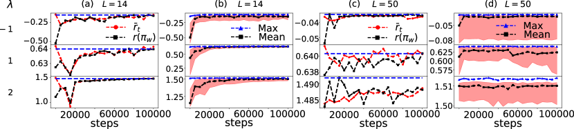
Figure S1: Training Procedure and Learning Curves (ASEP) (a) For each bias, with $\lambda=-1,1,2$ shown here, policies and value-functions are produced via gradient ascent SM . These are initiated at random for $L=4$ with $\chi=16$ and trained for $10^{6}$ steps. Every $5000$ training steps, the average-reward of the policy is evaluated over $10^{4}$ steps (black squares) and the weights of the policy (which we call a “snapshot” for that time) are stored. The evaluated values can be compared to the training estimate of $r(\pi)$ (red circles), which tends to overestimate $r(\pi)$ initially. The policy snapshot with the highest evaluated $r$ (blue dashed line) is used to initiate the policy for higher values of $L$. This is repeated every $\Delta L=2$ up to $L=50$, with the $L=14$ case shown here. (b) For each bias, several policies (here six) are independently trained via the same procedure from different random initial conditions. This produces a distribution of evaluated average-rewards, here represented by the median (black squares) and inter-quartile range (red-shaded region). The policy with the maximum average-reward at each $L$ is selected as the optimal dynamics (blue triangles). (c) Panel (a) is repeated here for the final $L=50$. As can be seen, the scale of change is now much smaller, and the learning curves appear nosier as a result (the learning rate is kept fixed throughout). (d) The distribution of evaluated $r$ across parallel agents for $L=50$ is again much tighter than with $L=14$, though appears nosier as a result.

References

- White (1992) S. R. White, Phys. Rev. Lett. 69, 2863 (1992).
- White (1993) S. R. White, Phys. Rev. B 48, 10345 (1993).
- Schollwöck (2011) U. Schollwöck, Ann. Phys. 326, 96 (2011).
- Eisert et al. (2010) J. Eisert, M. Cramer, and M. B. Plenio, Rev. Mod. Phys. 82, 277 (2010).
- Eisert (2013) J. Eisert, Modeling and Simulation 3, 520 (2013), arXiv:1308.3318 .
- Montangero (2018) S. Montangero, Introduction to Tensor Network Methods (Springer International Publishing, 2018).
- Orús (2019) R. Orús, Nature Rev. Phys. 1, 538 (2019).
- Stoudenmire and Schwab (2016) E. Stoudenmire and D. J. Schwab, in Advances in Neural Information Processing Systems 29, edited by D. D. Lee, M. Sugiyama, U. V. Luxburg, I. Guyon, and R. Garnett (Curran Associates, Inc., 2016) pp. 4799–4807, arXiv:1605.05775 .
- Liu et al. (2018) Y. Liu, X. Zhang, M. Lewenstein, and S.-J. Ran, arXiv:1803.09111 (2018).
- Sun et al. (2019) Z.-Z. Sun, C. Peng, D. Liu, S.-J. Ran, and G. Su, arXiv:1903.10742 (2019).
- Roberts et al. (2019) C. Roberts, A. Milsted, M. Ganahl, A. Zalcman, B. Fontaine, Y. Zou, J. Hidary, G. Vidal, and S. Leichenauer, arXiv:1905.01330 (2019).
- Ghahramani and Jordan (1997) Z. Ghahramani and M. I. Jordan, Mach. Learn. 29, 245 (1997).
- Efthymiou et al. (2019) S. Efthymiou, J. Hidary, and S. Leichenauer, arXiv:1906.06329 (2019).
- Stoudenmire (2018) E. M. Stoudenmire, Quantum Sci. Technol. 3, 034003 (2018).
- Han et al. (2018) Z.-Y. Han, J. Wang, H. Fan, L. Wang, and P. Zhang, Phys. Rev. X 8, 031012 (2018).
- Gao et al. (2019) Z.-F. Gao, S. Cheng, R.-Q. He, Z. Y. Xie, H.-H. Zhao, Z.-Y. Lu, and T. Xiang, arXiv:1904.06194 (2019).
- Levine et al. (2019) Y. Levine, O. Sharir, N. Cohen, and A. Shashua, Phys. Rev. Lett. 122, 065301 (2019).
- Guo et al. (2018) C. Guo, Z. Jie, W. Lu, and D. Poletti, Phys. Rev. E 98, 042114 (2018).
- Glasser et al. (2018) I. Glasser, N. Pancotti, and J. I. Cirac, arXiv:1806.05964 (2018).
- Glasser et al. (2019) I. Glasser, R. Sweke, N. Pancotti, J. Eisert, and I. Cirac, in Advances in Neural Information Processing Systems 32, edited by H. Wallach, H. Larochelle, A. Beygelzimer, F. Alche-Buc, E. Fox, and R. Garnett (Curran Associates, Inc., 2019) pp. 1496–1508.
- Sutton and Barto (2018) R. S. Sutton and A. G. Barto, Reinforcement Learning: An Introduction (MIT Press, 2018).
- Mnih et al. (2015) V. Mnih, K. Kavukcuoglu, D. Silver, A. A. Rusu, J. Veness, M. G. Bellemare, A. Graves, M. Riedmiller, A. K. Fidjeland, G. Ostrovski, S. Petersen, C. Beattie, A. Sadik, I. Antonoglou, H. King, D. Kumaran, D. Wierstra, S. Legg, and D. Hassabis, Nature 518, 529 (2015).
- Haarnoja et al. (2018) T. Haarnoja, A. Zhou, K. Hartikainen, G. Tucker, S. Ha, J. Tan, V. Kumar, H. Zhu, A. Gupta, P. Abbeel, and S. Levine, arXiv:1812.05905 (2018).
- Silver et al. (2016) D. Silver, A. Huang, C. J. Maddison, A. Guez, L. Sifre, G. van den Driessche, J. Schrittwieser, I. Antonoglou, V. Panneershelvam, M. Lanctot, S. Dieleman, D. Grewe, J. Nham, N. Kalchbrenner, I. Sutskever, T. Lillicrap, M. Leach, K. Kavukcuoglu, T. Graepel, and D. Hassabis, Nature 529, 484 (2016).
- Schulman et al. (2015) J. Schulman, S. Levine, P. Abbeel, M. I. Jordan, and P. Moritz, in International Conference on Machine Learning (2015).
- Wang et al. (2019) T. Wang, X. Bao, I. Clavera, J. Hoang, Y. Wen, E. Langlois, S. Zhang, G. Zhang, P. Abbeel, and J. Ba, arXiv:1907.02057 (2019).
- Metz and Bukov (2022) F. Metz and M. Bukov, arXiv:2201.11790 (2022).
- Mahajan et al. (2021) A. Mahajan, M. Samvelyan, L. Mao, V. Makoviychuk, A. Garg, J. Kossaifi, S. Whiteson, Y. Zhu, and A. Anandkumar, arXiv:2106.00136 (2021).
- Garrahan (2016) J. P. Garrahan, J. Stat. Mech. 2016, 073208 (2016).
- Garrahan (2018) J. P. Garrahan, Physica A 504, 130 (2018).
- Jack and Sollich (2015) R. L. Jack and P. Sollich, Eur. Phys. J. Spec. Top. 224, 2351 (2015).
- Jack (2019) R. L. Jack, (2019), arXiv:1910.09883 .
- Chetrite and Touchette (2015a) R. Chetrite and H. Touchette, Ann Henri Poincaré (2015a).
- Casert et al. (2021) C. Casert, T. Vieijra, S. Whitelam, and I. Tamblyn, Phys. Rev. Lett. 127, 120602 (2021).
- Majumdar and Orland (2015) S. N. Majumdar and H. Orland, J. Stat. Mech. 2015, P06039 (2015).
- Chetrite and Touchette (2015b) R. Chetrite and H. Touchette, J. Stat. Mech. 2015, P12001 (2015b).
- Bolhuis et al. (2002) P. G. Bolhuis, D. Chandler, C. Dellago, and P. L. Geissler, Annu. Rev. Phys. Chem. 53, 291 (2002).
- Giardinà et al. (2006) C. Giardinà, J. Kurchan, and L. Peliti, Phys. Rev. Lett. 96, 120603 (2006).
- Giardina et al. (2011) C. Giardina, J. Kurchan, V. Lecomte, and J. Tailleur, J. Stat. Phys. 145, 787 (2011).
- Cérou and Guyader (2007) F. Cérou and A. Guyader, Stoch. Anal. Appl. 25, 417 (2007).
- Lecomte and Tailleur (2007) V. Lecomte and J. Tailleur, J. Stat. Mech. 2007, P03004 (2007).
- Whitelam et al. (2020) S. Whitelam, D. Jacobson, and I. Tamblyn, J. Chem. Phys. 153, 044113 (2020).
- De Bruyne et al. (2021) B. De Bruyne, S. N. Majumdar, and G. Schehr, Phys. Rev. E 104, 024117 (2021).
- Bruyne et al. (2021a) B. D. Bruyne, S. N. Majumdar, H. Orland, and G. Schehr, J. Stat. Mech. 2021, 123204 (2021a).
- Bruyne et al. (2021b) B. D. Bruyne, S. N. Majumdar, and G. Schehr, J. Phys. A 54, 385004 (2021b).
- De Bruyne et al. (2022) B. De Bruyne, S. N. Majumdar, and G. Schehr, Phys. Rev. Lett. 128, 200603 (2022).
- Pozzoli and Bruyne (2022) G. Pozzoli and B. D. Bruyne, arXiv:2207.06865 (2022).
- Rose et al. (2021) D. C. Rose, J. F. Mair, and J. P. Garrahan, New J. Phys. 23, 013013 (2021).
- Das and Limmer (2019) A. Das and D. T. Limmer, J. Chem. Phys. 151, 244123 (2019).
- Das et al. (2021) A. Das, D. C. Rose, J. P. Garrahan, and D. T. Limmer, J. Chem. Phys. 155, 134105 (2021).
- Das et al. (2022) A. Das, B. Kuznets-Speck, and D. T. Limmer, Phys. Rev. Lett. 128, 028005 (2022).
- Borkar et al. (2003) V. S. Borkar, S. Juneja, and A. A. Kherani, Commun. Inf. Syst. 3, 259 (2003).
- Ferré and Touchette (2018) G. Ferré and H. Touchette, J. Stat. Phys. 172, 1525 (2018).
- Yan et al. (2022) J. Yan, H. Touchette, and G. M. Rotskoff, Phys. Rev. E 105, 024115 (2022).
- Yan and Rotskoff (2022) J. Yan and G. M. Rotskoff, J. Chem. Phys. 157, 074101 (2022).
- Nemoto and Sasa (2014) T. Nemoto and S.-i. Sasa, Phys. Rev. Lett. 112, 090602 (2014).
- Nemoto et al. (2017) T. Nemoto, R. L. Jack, and V. Lecomte, Phys. Rev. Lett. 118, 115702 (2017).
- Kappen and Ruiz (2016) H. J. Kappen and H. C. Ruiz, J. Stat. Phys. 162, 1244 (2016).
- Bolhuis et al. (2022) P. G. Bolhuis, Z. F. Brotzakis, and B. G. Keller, arXiv:2207.04558 (2022).
- Holdijk et al. (2022) L. Holdijk, Y. Du, F. Hooft, P. Jaini, B. Ensing, and M. Welling, arXiv:2207.02149 (2022).
- Note (1) In some scenarios all actions maybe possible from any state, or the desired constraint itself is unknown and must be learnt by penalising the policy when disallowed actions are selected, in which case we can simply set .
- (62) see Supplemental Material for details .
- Bradbury et al. (2018) J. Bradbury, R. Frostig, P. Hawkins, M. J. Johnson, C. Leary, D. Maclaurin, G. Necula, A. Paszke, J. VanderPlas, S. Wanderman-Milne, and Q. Zhang, “JAX: composable transformations of Python+NumPy programs,” (2018).
- Helms et al. (2019) P. Helms, U. Ray, and G. K.-L. Chan, Phys. Rev. E 100, 022101 (2019).
- Bañuls and Garrahan (2019) M. C. Bañuls and J. P. Garrahan, Phys. Rev. Lett. 123, 200601 (2019).
- Helms and Chan (2020) P. Helms and G. K.-L. Chan, Phys. Rev. Lett. 125, 140601 (2020).
- Causer et al. (2020) L. Causer, I. Lesanovsky, M. C. Bañuls, and J. P. Garrahan, Phys. Rev. E 102, 052132 (2020).
- Causer et al. (2021) L. Causer, M. C. Bañuls, and J. P. Garrahan, Phys. Rev. E 103, 062144 (2021).
- Causer et al. (2022a) L. Causer, M. C. Bañuls, and J. P. Garrahan, Phys. Rev. Lett. 128, 090605 (2022a).
- Causer et al. (2022b) L. Causer, J. P. Garrahan, and A. Lamacraft, Phys. Rev. E 106, 014128 (2022b).
- Fishman et al. (2022) M. Fishman, S. White, and E. Stoudenmire, SciPost Physics Codebases (2022), 10.21468/scipostphyscodeb.4.
- DeepMind (2022) DeepMind, “Using jax to accelerate our research,” (2022).
- Terry et al. (2020) J. K. Terry, B. Black, N. Grammel, M. Jayakumar, A. Hari, R. Sulivan, L. Santos, R. Perez, C. Horsch, C. Dieffendahl, N. L. Williams, Y. Lokesh, R. Sullivan, and P. Ravi, arXiv:2009.14471 (2020).
- Van Rossum and Drake (2009) G. Van Rossum and F. L. Drake, Python 3 Reference Manual (CreateSpace, Scotts Valley, CA, 2009).
- Harris et al. (2020) C. R. Harris, K. J. Millman, S. J. van der Walt, R. Gommers, P. Virtanen, D. Cournapeau, E. Wieser, J. Taylor, S. Berg, N. J. Smith, R. Kern, M. Picus, S. Hoyer, M. H. van Kerkwijk, M. Brett, A. Haldane, J. F. del Río, M. Wiebe, P. Peterson, P. Gérard-Marchant, K. Sheppard, T. Reddy, W. Weckesser, H. Abbasi, C. Gohlke, and T. E. Oliphant, Nature 585, 357 (2020).
- The pandas development team (2022) The pandas development team, (2022), 10.5281/zenodo.7093122.
- Hunter (2007) J. D. Hunter, Comput. Sci. Eng. 9, 90 (2007).
- Collette (2013) A. Collette, Python and HDF5 (O’Reilly, 2013).
- Bezanson et al. (2017) J. Bezanson, A. Edelman, S. Karpinski, and V. B. Shah, SIAM Rev. Soc. Ind. Appl. Math. 59, 65 (2017).
- HDF (2022) “HDF5.jl,” (2022).
- Gillman and Rose (2022) E. Gillman and D. C. Rose, “Acten, actor critic with tensor networks,” https://github.com/RL-with-TNs/acten_code (2022).