Global Weighted Tensor Nuclear Norm for Tensor Robust Principal Component Analysis

Abstract

Tensor Robust Principal Component Analysis (TRPCA), which aims to recover a low-rank tensor corrupted by sparse noise, has attracted much attention in many real applications. This paper develops a new Global Weighted TRPCA method (GWTRPCA), which is the first approach simultaneously considers the significance of intra-frontal slice and inter-frontal slice singular values in the Fourier domain. Exploiting this global information, GWTRPCA penalizes the larger singular values less and assigns smaller weights to them. Hence, our method can recover the low-tubal-rank components more exactly. Moreover, we propose an effective adaptive weight learning strategy by a Modified Cauchy Estimator (MCE) since the weight setting plays a crucial role in the success of GWTRPCA. To implement the GWTRPCA method, we devise an optimization algorithm using an Alternating Direction Method of Multipliers (ADMM) method. Experiments on real-world datasets validate the effectiveness of our proposed method.

Introduction

Real-world data such as images, texts, videos and bioinformatics are usually high-dimensional and can be approximated by low-rank structures. Exploiting these low-rank structures from high-dimensional data is an essential problem in many real applications, e.g., face recogniton (Pang et al. 2020), collaborative filtering (Koren 2008) and image denoising (Bouwmans et al. 2018). Robust Principal Component Analysis (RPCA) (Candès et al. 2011), one of the most representative methods in this problem, has attracted much attention. It aims to separate the observed data matrix $\mathbf{X}\in\mathbb{R}^{d_{1}\times d_{2}}$ into a low-rank matrix $\mathbf{L}$ and a sparse matrix $\mathbf{E}$, where $\mathbf{L}$ denotes clean data and $\mathbf{E}$ denotes the noise. It has been proved in (Candès et al. 2011) that $\mathbf{L}$ and $\mathbf{E}$ can be exactly recovered with high probability under proper conditions by solving the following convex problem

$$\min_{\mathbf{L},\mathbf{E}\in\mathbb{R}^{d_{1}\times d_{2}}}\|\mathbf{L}\|_{*}+\lambda\|\mathbf{E}\|_{1}\leavevmode\nobreak\ \leavevmode\nobreak\ \text{s.t.}\leavevmode\nobreak\ \leavevmode\nobreak\ \mathbf{X}=\mathbf{L}+\mathbf{E},$$ (1)

where $\lambda>0$ is the regularization parameter, $\|\mathbf{\cdot}\|_{*}$ and $\|\mathbf{\cdot}\|_{1}$ denote the nuclear norm (sum of the singular values) and $\ell_{1}$-norm (sum of the absolute values of all entries), respectively.

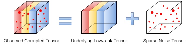
Figure 1: An illustration of Tensor Robust Principal Component Analysis.

One major drawback of RPCA is that it can only handle 2-order (matrix) data. However, multi-dimensional data, termed as tensor data (Kolda and Bader 2009), is widely used in many real applications (Gao et al. 2020; Mu et al. 2020). For example, a color image is a 3-order tensor with column, row and color modes; a gray scale video is indexed by two spatial variables and one temporal variable. To handle the tensor data, RPCA needs to restructure the high-order tensor data into a matrix and thus ignores the information embedded in multi-dimensional structures. The information loss can lead to performance degradation and an inexact recovery.

To alleviate this problem, many Tensor RPCA methods have been proposed, which aim to separate the observed tensor data $\mathcal{X}$ into a clean low-rank tensor $\mathcal{L}$ and a sparse noise tensor $\mathcal{E}$ (An illustration can be seen in Fig. 1). Liu et al. (2013) initially extended the matrix nuclear norm to tensors by proposing Sum of Nuclear Norms (SNN). It is defined as $\sum_{i}{\|\mathbf{X}^{\{i\}}\|}_{*}$, where $\mathbf{X}^{\{i\}}$ is the mode-$i$ matricization of $\mathcal{X}$ (Liu et al. 2013). The SNN based Tensor RPCA method (Huang et al. 2015) can be formulated as

$$\min_{\mathcal{L},\mathcal{E}\in\mathbb{R}^{d_{1}\times d_{2}\times d_{3}}}\sum_{i=1}^{k}\lambda_{i}{\|{\mathbf{L}^{\{i\}}}\|}_{*}+{\|\mathcal{E}\|}_{1}\leavevmode\nobreak\ \leavevmode\nobreak\ \text{s.t.}\leavevmode\nobreak\ \leavevmode\nobreak\ \mathcal{X}=\mathcal{L}+\mathcal{E},$$ (2)

where $\lambda_{i}>0$ are regularization parameters. Although the SNN based Tensor RPCA method can guarantee the recovery, the algorithm is nonconvex. To overcome this shortcoming, Lu et al. (2020) proposed the Tensor Robust Principal Component (TRPCA) method with a new tensor nuclear norm, which is motivated by the tensor Singular Value Decomposition (t-SVD) (Kilmer and Martin 2011) :

$$\min_{\mathcal{L},\mathcal{E}\in\mathbb{R}^{d_{1}\times d_{2}\times d_{3}}}\|\mathcal{L}\|_{*}+\lambda\|\mathcal{E}\|_{1}\leavevmode\nobreak\ \leavevmode\nobreak\ \text{s.t.}\leavevmode\nobreak\ \leavevmode\nobreak\ \mathcal{X}=\mathcal{L}+\mathcal{E},$$ (3)

where $\|\cdot\|_{*}$ denotes the tensor nuclear norm (TNN).

Inspired by TNN defined in TRPCA, many improvements of TRPCA have been proposed. Gao et al. (2021) presented an Enhanced TRPCA (ETRPCA) method, which defines a weighted tensor Schatten p-norm to deal with the difference between singular values of tensor data. Wang et al. (2020) developed a Frequency-Filtered TRPCA mehtod. This method defines a frequency-filtered TNN, which utilizes the prior knowledge between different frequency bands. Besides, Liu, Chen, and Zhu (2018) indicated that TRPCA fails to employ the low-rank structure in the third mode and extending TNN with core matrix. Jiang et al. (2020) defined a partial sum of tubal nuclear norm (PSTNN) of a tensor, which is a surrogate of the tensor tubal multi-rank. By minimizing PSTNN, the smaller singular values are shrinked while the larger singular values are not. Additionally, TNN may over-penalize the large singular values of tensor data (Li and Ma 2021). Kong, Xie, and Lin (2018) proposed t-Schatten-$p$ quasi-norm to improve TNN, which is non-convex when $0<p<1$ and can be a better approximationof the $l_{1}$ norm of tensor multi-rank. Besides, a new t-Gamma tensor quasi-norm as a non-convex regularzation was defined by Cai et al. (2019) to approximate the low-rank component.

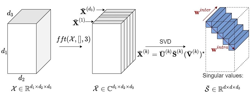
Figure 2: An illustration of the global weight to singular values of an $d_{1}\times d_{2}\times d_{3}$ tensor in the Fourier domain ($d=\min(d_{1},d_{2})$; $\mathbf{w}^{intra}\in\mathbb{R}^{d}$: weight vector for intra-frontal slice singular values; $\mathbf{w}^{inter}\in\mathbb{R}^{d_{3}}$: weight vector for inter-frontal slice singular values).

Motivation and Contribution

Despite the theoretical guarantee and emperical success, TRPCA treats all singular values of tensor data equally and regularizes different singular values with the same weights. It may cause an inexact estimation of the tubal rank of tensor data (Gao et al. 2021). Additionally, singular values usually have clear physical meanings in many real applications. For example, larger singular values are generally associated with some prominent information of the image. Hence, we should assign smaller weights for the larger singular values to efficiently preserve the prominent information.

To overcome the drawback of TRPCA, Enhanced TRPCA (ETRPCA) (Gao et al. 2021) assigns different weights to penalize distinct singular values. However, it only considers intra-frontal slice singular values. We observe that the decreasing property also holds on for inter-frontal slice singualr values (along the third dimension). As is shown in Fig. 2, we only exploit the local information of tensor singular values and neglect the inter-frontal slice weights when we just assign intra-frontal slice weights like ETRPCA. This can result in an inaccurate evaluation of weights and performance decline. To handle this problem, our method GWTRPCA defines a new Global Weighted TNN and can learn weights of different singular values more exactly.

The contributions of this paper are as follows:

• We propose a new weighted TNN, Global Weighted Tensor Nuclear Norm (GWTNN), which considers the significance of intra-frontal slice and inter-frontal slice singular values simultaneously in the Fourier domain. GWTNN can be a better surrogate of the tubal rank function.

• We put forward a new TRPCA method employing GWTNN termed Global Weighted Tensor Principle Component Analysis (GWTRPCA). We also devise an effective optimization algorithm for GWTRPCA based on the ADMM framework.

• We propose an adaptive weight learning strategy by a Modified Cauchy Estimator (MCE). We utilize the strategy to learn inter-frontal slice weights and further improve the performance of GWTRPCA.

Notations and Preliminaries

Notations

In this paper, we represent scalars, vectors, matrices and tensors using normal letters, boldface lower-case, upper-case letters and script letters, respectively. For a complex matrix $\mathbf{X}\in\mathbb{C}^{d_{1}\times d_{2}}$, $\mathbf{X}^{*}$ denote its conjugate transpose. We denote $\lceil t\rceil$ as the nearest integer more than or equal to t. For $t\in\{1,2,\cdots,n\}$, we denote it as $t\in[n]$. For brevity, we summarzie the main natations in Tab. 1.

T-Product

To define the tensor-tensor product (or t-product), we first introduce some useful tensor operators.

Definition 1

(The fold and unfold operators (Kilmer and Martin 2011)) For any 3-order tensor $\mathcal{X}\in\mathbb{R}^{d_{1}\times d_{2}\times d_{3}}$, we define

$$\textnormal{unfold}(\mathcal{X})=\begin{bmatrix}\mathbf{X}^{(1)}\\ \mathbf{X}^{(2)}\\ \vdots\\ \mathbf{X}^{(d_{3})}\\ \end{bmatrix},\leavevmode\nobreak\ \textnormal{fold}(\textnormal{unfold}(\mathcal{X}))=\mathcal{X}.$$ (4)

Definition 2

(The bcirc operator (Kilmer and Martin 2011)) The block circulant matrix of any 3-order tensor $\mathcal{X}\in\mathbb{R}^{d_{1}\times d_{2}\times d_{3}}$ is defined as

$$\textnormal{bcirc}(\mathcal{X})=\begin{bmatrix}\mathbf{X}^{(1)}&\mathbf{X}^{(d_{3})}&\cdots&\mathbf{X}^{(2)}\\ \mathbf{X}^{(2)}&\mathbf{X}^{(1)}&\cdots&\mathbf{X}^{(3)}\\ \vdots&\vdots&\ddots&\vdots\\ \mathbf{X}^{(d_{3})}&\mathbf{X}^{(2)}&\cdots&\mathbf{X}^{(1)}\\ \end{bmatrix}$$ (5)

where $\mathbf{X}^{(k)}$ denotes the $k$-th frontal slice of $\mathcal{X}$.

Definition 3

(T-product (Kilmer and Martin 2011)) The t-product of any two 3-order tensor $\mathcal{X}\in\mathbb{R}^{d_{1}\times d_{2}\times d_{3}}$ and $\mathcal{Y}\in\mathbb{R}^{d_{2}\times l\times d_{3}}$ is defined to be a tensor of size $d_{1}\times l\times d_{3}$

$$\mathcal{X}*\mathcal{Y}=\textnormal{fold}(\textnormal{bcirc}(\mathcal{X})\cdot\textnormal{unfold}(\mathcal{Y})).$$ (6)

In fact, the t-product $\mathcal{Z}=\mathcal{X}*\mathcal{Y}$ can be computed efficiently with the aid of $fft$ (Lu et al. 2020). Specifically, let $\bar{\mathcal{X}}=fft(\mathcal{X},[],3)$ and $\bar{\mathcal{Y}}=fft(\mathcal{Y},[],3)$. We can first calculate the $k$-th frontal slice of $\bar{\mathcal{Z}}$ as $\bar{\mathbf{Z}}^{(k)}=\bar{\mathbf{X}}^{(k)}\bar{\mathbf{Y}}^{(k)}$, where $\bar{\mathbf{X}}^{(k)}$ and $\bar{\mathbf{Y}}^{(k)}$ are the $k$-th frontal slice of $\bar{\mathcal{X}}$ and $\bar{\mathcal{Y}}$, respectively. Then we can obtain $\mathcal{Z}=ifft(\bar{\mathcal{Z}},[],3)$.

Notation	Description
$\mathcal{X}\in\mathbb{R}^{d_{1}\times d_{2}\times d_{3}}$	tensor data
$\mathcal{L}\in\mathbb{R}^{d_{1}\times d_{2}\times d_{3}}$	low-rank tensor
$\mathcal{S}\in\mathbb{R}^{d_{1}\times d_{2}\times d_{3}}$	sparse tensor
$\mathcal{X}_{ijk}$ or $\mathcal{X}(i,j,k)$	$(i,j,k)$-th entry of $\mathcal{X}$
$\mathcal{X}(i,:,:)$	$i$-th horizontal slice of $\mathcal{X}$
$\mathcal{X}(:,j,:)$	$j$-th lateral slice of $\mathcal{X}$
$\mathcal{X}(:,:,k)$ or $\mathbf{X}^{(k)}$	$k$-th frontal slice of $\mathcal{X}$
DFT	Discrete Fourier Transform
FFT	Fast Fourier Transform
$\bar{\mathcal{X}}\in\mathbb{C}^{d_{1}\times d_{2}\times d_{3}}$	DFT of $\mathcal{X}$ along the $3$-rd dimension
$fft(\mathcal{X},[],3)$	FFT of $\mathcal{X}$ along the $3$-rd dimension
$\|\mathcal{X}\|_{*}$	Tensor Nuclear Norm
$\|\mathcal{X}\|_{1}$	Tensor $\ell_{1}$ Norm
TNN	Tensor Nuclear Norm
GWTNN	Global Weighted TNN
$[n]$	set $\{1,2,\cdots,n\}$

Table 1: Key notations used in this paper.

T-SVD and Tensor Nuclear Norm

Before introducing the Tensor-SVD (T-SVD) and Tensor Nuclear Norm (TNN), it is necessary to introduce some useful definitions associated with tensors.

Definition 4

(Conjugate transpose (Kilmer and Martin 2011)) The conjugate transpose of a tensor $\mathcal{X}\in\mathbb{C}^{d_{1}\times d_{2}\times d_{3}}$ is the tensor $\mathcal{X}^{*}\in\mathbb{C}^{d_{2}\times d_{1}\times d_{3}}$ obtained by conjugate transposing each of the frontal slices and then reversing the order of the transposed frontal slices 2 through $d_{3}$.

Definition 5

(Identity tensor (Kilmer and Martin 2011)) The identity tensor $\mathcal{I}\in\mathbb{R}^{d\times d\times d_{3}}$ is the tensor with its first frontal slice being the $d\times d$ identity matrix, and other frontal slices being all zeros.

Definition 6

(Orthogonal tensor (Kilmer and Martin 2011)) A tensor $\mathcal{Q}\in\mathbb{R}^{d\times d\times d_{3}}$ is orthogonal if it satisfies $\mathcal{Q}^{*}*\mathcal{Q}=\mathcal{Q}*\mathcal{Q}^{*}=\mathcal{I}$.

Definition 7

(F-diagonal tensor (Kilmer and Martin 2011)) A tensor is called f-diagonal if each of its frontal slices is a diagonal matrix.

Definition 8

(Tensor Singular Value Decomposition, T-SVD (Kilmer and Martin 2011)) The tensor $\mathcal{X}\in\mathbb{R}^{d_{1}\times d_{2}\times d_{3}}$ can be factorized as

$$\mathcal{X}=\mathcal{U}*\mathcal{S}*\mathcal{V}^{*},$$ (7)

where $\mathcal{U}\in\mathbb{R}^{d_{1}\times d_{1}\times d_{3}}$, $\mathcal{V}\in\mathbb{R}^{d_{2}\times d_{2}\times d_{3}}$ are orthogonal, and $\mathcal{S}\in\mathbb{R}^{d_{1}\times d_{2}\times d_{3}}$ is an f-diagonal tensor.

Definition 9

(Tensor Nuclear Norm (Lu et al. 2020)) Let $\mathcal{X}=\mathcal{U}*\mathcal{S}*\mathcal{V}^{*}$ be the t-SVD of $\mathcal{X}\in\mathbb{R}^{d_{1}\times d_{2}\times d_{3}}$ and $d=\min(d_{1},d_{2})$. The tensor nuclear norm of $\mathcal{X}$ is defined as

$$\|\mathcal{X}\|_{*}=\sum_{i=1}^{d}\mathcal{S}(i,i,1)=\frac{1}{d_{3}}\sum_{k=1}^{d_{3}}\sum_{i=1}^{d}\sigma_{i}\left(\bar{\mathbf{X}}^{(k)}\right),$$ (8)

where $\sigma_{i}\left(\bar{\mathbf{X}}^{(k)}\right)$ is the $i$-th singular value of $\bar{\mathbf{X}}^{(k)}$.

Proposed Method

Global Weighted Tensor Nuclear Norm

It is known that the singular values of a matrix have the decreasing property. Given any tensor $\mathcal{X}\in\mathbb{R}^{d_{1}\times d_{2}\times d_{3}}$ and $d=\min\{d_{1},d_{2}\}$, let $\bar{\mathcal{X}}$ be the result by applying DFT (Discrete Fourier Transform) on $\mathcal{X}$ along the third dimension, $\bar{\mathbf{X}}^{(k)}$ is the $k$-th frontal slice of $\bar{\mathcal{X}}$, and $\sigma_{i}\left(\bar{\mathbf{X}}^{(k)}\right)$ is the $i$-th singular value of $\bar{\mathbf{X}}^{(k)}$. Thus, for any $k\in[d_{3}]$, the singular values in the $k$-th frontal slice $\bar{\mathbf{X}}^{(k)}$ have the same decreasing property, i.e.,

$$\sigma_{1}\left(\bar{\mathbf{X}}^{(k)}\right)\geq\sigma_{2}\left(\bar{\mathbf{X}}^{(k)}\right)\geq\cdots\geq\sigma_{d}\left(\bar{\mathbf{X}}^{(k)}\right)\geq 0$$ (9)

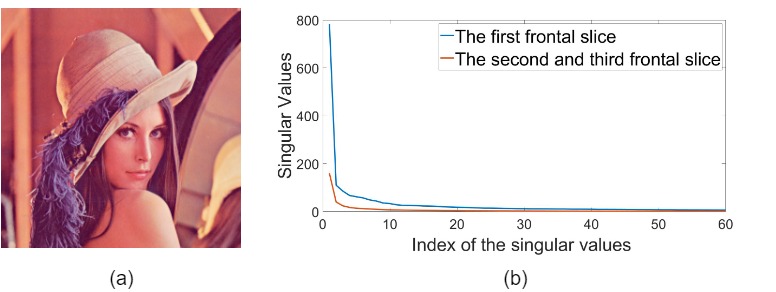
Figure 3: Illustration of the decreasing property of the inter-frontal slice singular values in the Fourier domain. (a) A color image can be modeled as a tensor $\mathcal{M}\in\mathbb{R}^{512\times 512\times 3}$; (b) plot of the first 60 singular values in the first, second and third frontal slice of $\bar{\mathcal{M}}$, respectively. Note that the singular values in the 2nd frontal slice are equal to those in the 3rd due to the conjugate symmetry of FFT.

The decreasing property also holds on when we consider the inter-frontal slice (across different frontal slices) singular values. As is shown in Fig. 3, the singular values in the first frontal slice tend to be larger than those in the second and third frontal slice for a 3-order tensor $\bar{\mathcal{M}}$ in the Fourier domain. Otherwise, we observe that the singular values in the second frontal slice are equal to those in the third frontal slice. This can be due to the property of DFT. Hence, the singular values of distinct frontal slices $\bar{\mathcal{X}}^{(k)}$ have another interesting property, i.e.,

$$\sum_{i=1}^{d}\sigma_{i}\left(\bar{\mathbf{X}}^{(1)}\right)\geq\cdots\geq\sum_{i=1}^{d}\sigma_{i}\left(\bar{\mathbf{X}}^{(\left\lceil\frac{d_{3}+1}{2}\right\rceil)}\right)\geq 0$$ (10)

$$\sum_{i=1}^{d}\sigma_{i}\left(\bar{\mathbf{X}}^{(k)}\right)=\sum_{i=1}^{d}\sigma_{i}\left(\bar{\mathbf{X}}^{(d_{3}-k+2)}\right),k=\left\lceil\frac{d_{3}+1}{2}\right\rceil+1,\cdots,d_{3}$$ (11)

Now we simultaneously consider the decreasing property of intra-frontal slice and inter-frontal slice singular values. Based on the global decreasing property, we can assign different weights to distinct singular values and give a better surrogate of the tubal rank with a new weighted tensor nuclear norm. Thus, we have the following definiton of Global Weighted Tensor Nuclear Norm (GWTNN).

It is worth noting that ETRPCA proposes the weighted tensor Schatten $p$-norm (WTSN) $\|\mathcal{X}\|_{\mathbf{w},S_{p}}=\left(\sum_{k=1}^{d_{3}}\sum_{i=1}^{d}w_{i}\sigma_{i}^{p}\left(\bar{\mathbf{X}}^{(k)}\right)\right)^{\frac{1}{p}}$ for $p>0$. When we overlook the differences of inter-frontal slice singular values and equalize the weights $w_{k}^{inter}=1$, GWTNN reduces to a special case of WTSN when $p=1$. Compared to WTSN, GWTNN possesses two advantages: First, GWTNN can be seen as a generalization of WTSN. GWTNN can approximate the tubal rank function more exactly and maintain the flexibility to solve different practical problems. Second, our proposed GWTNN considers the importance of different frontal slices in the Fourier domain. It can perserve the significant components in DFT, consequently improving the recovery performance.

Optimization

In this part, we develop an efficient optimization algorithm based on the ADMM framework.

The Lagrangian function of the GWTRPCA method (LABEL:eq:GWTRPCA) is formulated as

$$\begin{split}L({\mathcal{L}},{\mathcal{E}},\mathcal{Y},\mu)=&\|{\mathcal{L}}\|_{\mathbin{\mathchoice{\ooalign{$\displaystyle\vbox{\hbox{\scalebox{0.77778}{$\displaystyle\bigcirc$}}}$\cr$\displaystyle*$\cr}}{\ooalign{$\textstyle\vbox{\hbox{\scalebox{0.77778}{$\textstyle\bigcirc$}}}$\cr$\textstyle*$\cr}}{\ooalign{$\scriptstyle\vbox{\hbox{\scalebox{0.77778}{$\scriptstyle\bigcirc$}}}$\cr$\scriptstyle*$\cr}}{\ooalign{$\scriptscriptstyle\vbox{\hbox{\scalebox{0.77778}{$\scriptscriptstyle\bigcirc$}}}$\cr$\scriptscriptstyle*$\cr}}}}+\lambda\|{\mathcal{E}}\|_{1}\\ &+\frac{\mu}{2}\left\|{\mathcal{L}}+{\mathcal{E}}-\mathcal{X}+\mathcal{Y}/\mu\right\|_{F}^{2}-\frac{\mu}{2}\|\mathcal{Y}/\mu\|_{F}^{2}.\end{split}$$ (12)

The variables can be updated alternatively by fixing others in each iteration. Let ${\mathcal{E}}_{t}$, $\mathcal{Y}_{t}$, $\mathbf{w}^{iner}_{t}$ and $\mu_{t}$ be the value of ${\mathcal{E}}$, $\mathcal{Y}$, $\mathbf{w}^{iner}$ and $\mu$ in the $t$-th iteration, respectively.

Step 1: Update ${\mathcal{L}}$

$${\mathcal{L}}_{t+1}=\mathop{{\rm arg}\min}_{{\mathcal{L}}\in\mathbb{R}^{d_{1}\times d_{2}\times d_{3}}}\frac{1}{2}\left\|{\mathcal{L}}-\left(\mathcal{X}-{\mathcal{E}}_{t}-\mathcal{Y}_{t}/\mu_{t}\right)\right\|_{F}^{2}+\frac{1}{\mu_{t}}\|{\mathcal{L}}\|_{\mathbin{\mathchoice{\ooalign{$\displaystyle\vbox{\hbox{\scalebox{0.77778}{$\displaystyle\bigcirc$}}}$\cr$\displaystyle*$\cr}}{\ooalign{$\textstyle\vbox{\hbox{\scalebox{0.77778}{$\textstyle\bigcirc$}}}$\cr$\textstyle*$\cr}}{\ooalign{$\scriptstyle\vbox{\hbox{\scalebox{0.77778}{$\scriptstyle\bigcirc$}}}$\cr$\scriptstyle*$\cr}}{\ooalign{$\scriptscriptstyle\vbox{\hbox{\scalebox{0.77778}{$\scriptscriptstyle\bigcirc$}}}$\cr$\scriptscriptstyle*$\cr}}}}.$$ (13)

Algorithm 1 GWTRPCA

Input: Data tensor $\mathcal{X}\in\mathbb{R}^{d_{1}\times d_{2}\times d_{3}}$, weight vector $\mathbf{w}^{intra}\in\mathbb{R}^{d},d=\min\{d_{1},d_{2}\}$ and the parameter $\lambda$.
Initialize: ${\mathcal{L}}_{0}=0$, ${\mathcal{E}}_{0}=0$, $\mathcal{Y}_{0}=0$, $\mathbf{w}^{inter}=\mathbf{1}$, $\mu=10^{-2}$, $\rho=1.1$, $\mu_{\text{max}}=10^{7}$, and $\epsilon=10^{-6}$.

1:  while not convergence do

2:     Update ${\mathcal{L}}$ by Eq. (13);

3:     Update ${\mathcal{E}}$ by Eq. (17);

4:     Update the multipliers $\mathcal{Y}_{t+1}=\mathcal{Y}_{t}+\mu_{t}({\mathcal{L}}_{t+1}-{\mathcal{E}}_{t+1}-\mathcal{X})$;

5:     Update the parameter $\mu$ by $\mu_{t+1}=\min\{\rho\mu_{t},\mu_{\text{max}}\};$

6:     Check the convergence conditions: $\|\mathcal{X}-{\mathcal{E}}_{t+1}-{\mathcal{L}}_{t+1}\|_{\infty}<\epsilon.$

7:  end while

Output: ${\mathcal{L}}={\mathcal{L}}_{t+1}$, ${\mathcal{E}}={\mathcal{E}}_{t+1}$.

(a) Oringinal

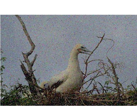
(b) Observed

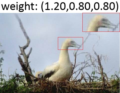
(c) PSNR=26.95

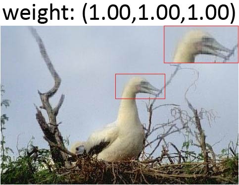
(d) PSNR=28.27

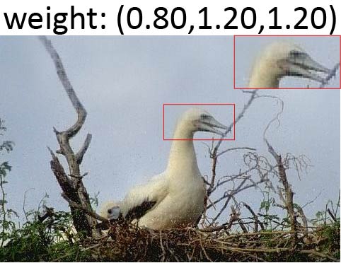
(e) PSNR=29.05

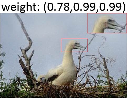
(f) PSNR=29.17

Figure 4: Recovery performance comparison of a test image under different weight settings. (a) Original image; (b) observed image with 10% corruption; (c)-(e) recovered images when we set $\mathbf{w}^{inter}=(1.20,0.80,0.80)$, $\mathbf{w}^{inter}=(1.0,1.0,1.0)$, $\mathbf{w}^{inter}=(0.80,1.20,1.20)$, respectively; (f) recovered image by GWTRPCA and the adaptively learned weight is $\mathbf{w}^{inter}=(0.78,0.99,0.99)$, which leads to the best recovery. Best viewed in ×2 sized color pdf file.

The problem above has a closed-form optimal solution. To derive the solution, we first introduce the following lemma about the solution to the Weighted Nuclear Norm Minimization (WNNM) problem of matrix data (Gu et al. 2017).

Lemma 1

(Gu et al. 2017) Given a data matrix $\mathbf{M}\in\mathbb{R}^{d_{1}\times d_{2}}$ and a weight vector $\mathbf{w}=[w_{1},\cdots,w_{d}]^{T}\in\mathbb{R}^{d}$ where $d=\min(d_{1},d_{2})$, let $\mathbf{M}=\mathbf{U}\mathbf{S}\mathbf{V}^{T}$ be the SVD of $\mathbf{M}$. Consider the WNNM problem

$$\mathbf{prox}_{\|\cdot\|_{\mathbf{w},*}}(\mathbf{M}):=\mathop{{\rm arg}\min}_{\mathbf{L}\in\mathbb{R}^{d_{1}\times d_{2}}}\frac{1}{2}\|\mathbf{L}-\mathbf{M}\|_{F}^{2}+\|\mathbf{L}\|_{\mathbf{w},*}$$ (14)

where $\mathbf{prox}_{\|\cdot\|_{\mathbf{w},*}}(\mathbf{M})$ denotes the proximal operator w.r.t. the weighted nuclear norm $\|\cdot\|_{\mathbf{w},*}$, $\|\mathbf{L}\|_{\mathbf{w},*}=\sum_{i=1}^{d}w_{i}\sigma_{i}(\mathbf{L})$. If the weights satisfy $0\leq w_{1}\leq\cdots\leq w_{d}$ , the global solution to (14) is

$$\mathbf{L}^{*}=\mathbf{prox}_{\|\cdot\|_{\mathbf{w},*}}(\mathbf{M})=\mathbf{U}\mathbf{P}_{\mathbf{w}}(\mathbf{S})\mathbf{V}^{T},$$

where $\mathbf{P}_{\mathbf{w}}(\mathbf{S})$ is a diagonal matrix with the same size of $\mathbf{S}$ and $(\mathbf{P}_{\mathbf{w}}(\mathbf{S}))_{ii}=(\mathbf{S}_{ii}-w_{i})_{+}$. Here $(x)_{+}=x$ if $x>0$ and $(x)_{+}=0$ otherwise.

For a tensor data $\mathcal{M}\in\mathbb{R}^{d_{1}\times d_{2}\times d_{3}}$ and a weight matrix $\mathbf{W}\in\mathbb{R}^{d_{3}\times d}$ where $d=\min(d_{1},d_{2})$, let $\mathcal{M}=\mathcal{U}*\mathcal{S}*\mathcal{V}^{*}$ be the T-SVD of $\mathcal{M}$. For each $\tau>0$, we can define a tensor operator $\mathcal{P}_{\tau}(\cdot)$ as

$$(\mathcal{P}_{\tau}(\bar{\mathcal{S}}))^{(k)}=\mathbf{P}_{w_{k}^{inter}\mathbf{w}^{intra}}\left(\bar{\mathbf{S}}^{(k)}\right),\leavevmode\nobreak\ k\in[d_{3}].$$

We can define the GWTNN proximal operator as follows

$$\mathbf{prox}_{\|\cdot\|_{\mathbin{\mathchoice{\ooalign{$\displaystyle\vbox{\hbox{\scalebox{0.77778}{$\displaystyle\bigcirc$}}}$\cr$\displaystyle*$\cr}}{\ooalign{$\textstyle\vbox{\hbox{\scalebox{0.77778}{$\textstyle\bigcirc$}}}$\cr$\textstyle*$\cr}}{\ooalign{$\scriptstyle\vbox{\hbox{\scalebox{0.77778}{$\scriptstyle\bigcirc$}}}$\cr$\scriptstyle*$\cr}}{\ooalign{$\scriptscriptstyle\vbox{\hbox{\scalebox{0.77778}{$\scriptscriptstyle\bigcirc$}}}$\cr$\scriptscriptstyle*$\cr}}}}}(\mathcal{M})=\mathcal{U}*ifft\left(\mathcal{P}_{\tau}(\bar{\mathcal{S}}),[],3\right)*\mathcal{V}^{*}.$$ (15)

Theorem 1

For any data tensor $\tau>0$, $\mathcal{M}\in\mathbb{R}^{d_{1}\times d_{2}\times d_{3}}$ and a weight matrix $\mathbf{W}\in\mathbb{R}^{d_{3}\times d}$, if the intra-frontal slice weight vector $\mathbf{w}^{intra}$ satisfies $0\leq w_{1}^{intra}\leq\cdots w_{d}^{intra}$, the GWTNN proximal operator (15) obeys

$$\mathbf{prox}_{\|\cdot\|_{\mathbin{\mathchoice{\ooalign{$\displaystyle\vbox{\hbox{\scalebox{0.77778}{$\displaystyle\bigcirc$}}}$\cr$\displaystyle*$\cr}}{\ooalign{$\textstyle\vbox{\hbox{\scalebox{0.77778}{$\textstyle\bigcirc$}}}$\cr$\textstyle*$\cr}}{\ooalign{$\scriptstyle\vbox{\hbox{\scalebox{0.77778}{$\scriptstyle\bigcirc$}}}$\cr$\scriptstyle*$\cr}}{\ooalign{$\scriptscriptstyle\vbox{\hbox{\scalebox{0.77778}{$\scriptscriptstyle\bigcirc$}}}$\cr$\scriptscriptstyle*$\cr}}}}}(\mathcal{M})=\mathop{{\rm arg}\min}_{{\mathcal{L}}\in\mathbb{R}^{d_{1}\times d_{2}\times d_{3}}}\frac{1}{2}\|{\mathcal{L}}-\mathcal{M}\|_{F}^{2}+\tau\|{\mathcal{L}}\|_{\mathbin{\mathchoice{\ooalign{$\displaystyle\vbox{\hbox{\scalebox{0.77778}{$\displaystyle\bigcirc$}}}$\cr$\displaystyle*$\cr}}{\ooalign{$\textstyle\vbox{\hbox{\scalebox{0.77778}{$\textstyle\bigcirc$}}}$\cr$\textstyle*$\cr}}{\ooalign{$\scriptstyle\vbox{\hbox{\scalebox{0.77778}{$\scriptstyle\bigcirc$}}}$\cr$\scriptstyle*$\cr}}{\ooalign{$\scriptscriptstyle\vbox{\hbox{\scalebox{0.77778}{$\scriptscriptstyle\bigcirc$}}}$\cr$\scriptscriptstyle*$\cr}}}}.$$ (16)

Proof 1

Please see the proof in Supplementary matrial B due to space limitation.

Step 2: Update ${\mathcal{E}}$

$${\mathcal{E}}_{t+1}=\mathop{{\rm arg}\min}_{{\mathcal{E}}\in\mathbb{R}^{d_{1}\times d_{2}\times d_{3}}}\frac{1}{2}\left\|{\mathcal{E}}-\left(\mathcal{X}-{\mathcal{L}}_{t+1}-\mathcal{Y}_{t}/\mu_{t}\right)\right\|_{F}^{2}+\frac{\lambda}{\mu}\|{\mathcal{E}}\|_{1}.$$ (17)

The problem above has a closed-form solution. Inspired by soft-thresholding operator, we have

$$\mathcal{E}_{t+1}=\mathrm{T}_{\frac{\lambda}{\mu_{t}}}\left(\mathcal{H}_{t+1}\right),\mathcal{H}_{t+1}=\mathcal{X}-{\mathcal{L}}_{t+1}-\mathcal{Y}_{t}/\mu_{t},$$ (18)

where the $(i,j,k)-$th element of $\mathrm{T}_{\frac{\lambda}{\mu_{t}}}\left(\mathcal{H}_{t+1}\right)$ is $sign\left(\left(\mathcal{H}_{t+1}\right)_{ijk}\right)\cdot\max\left(\left|\left(\mathcal{H}_{t+1}\right)_{ijk}\right|-\lambda/\mu_{t},0\right).$

Step 3: Update $\mathcal{Y}$ and $\mu$

$$\mathcal{Y}_{t+1}=\mathcal{Y}_{t}+\mu_{t}({\mathcal{L}}_{t+1}-{\mathcal{E}}_{t+1}-\mathcal{X}),\mu_{t+1}=\min\{\rho\mu_{t},\mu_{\text{max}}\}.$$

(a) Original

(b) Observed

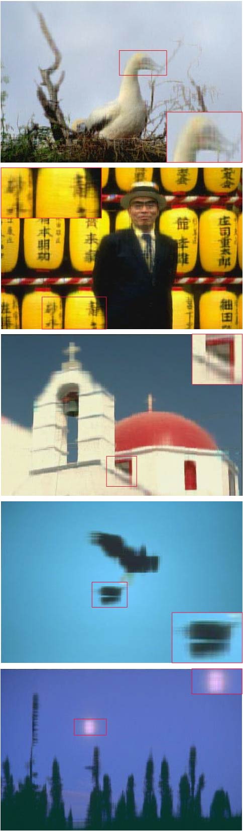
(c) RPCA

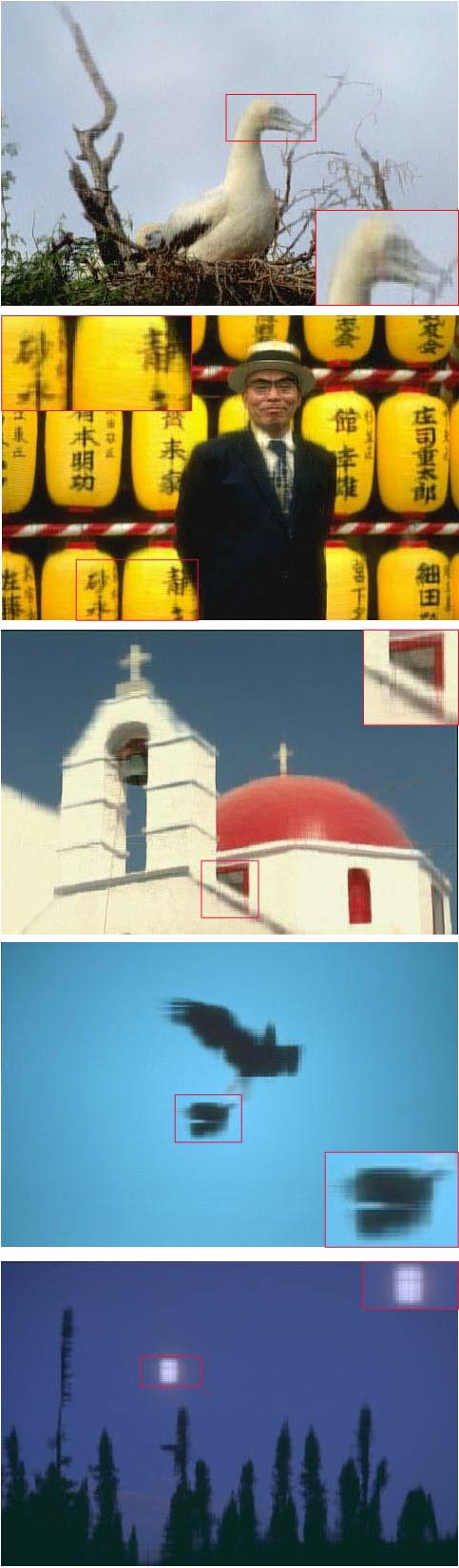
(d) SNN

(e) TRPCA

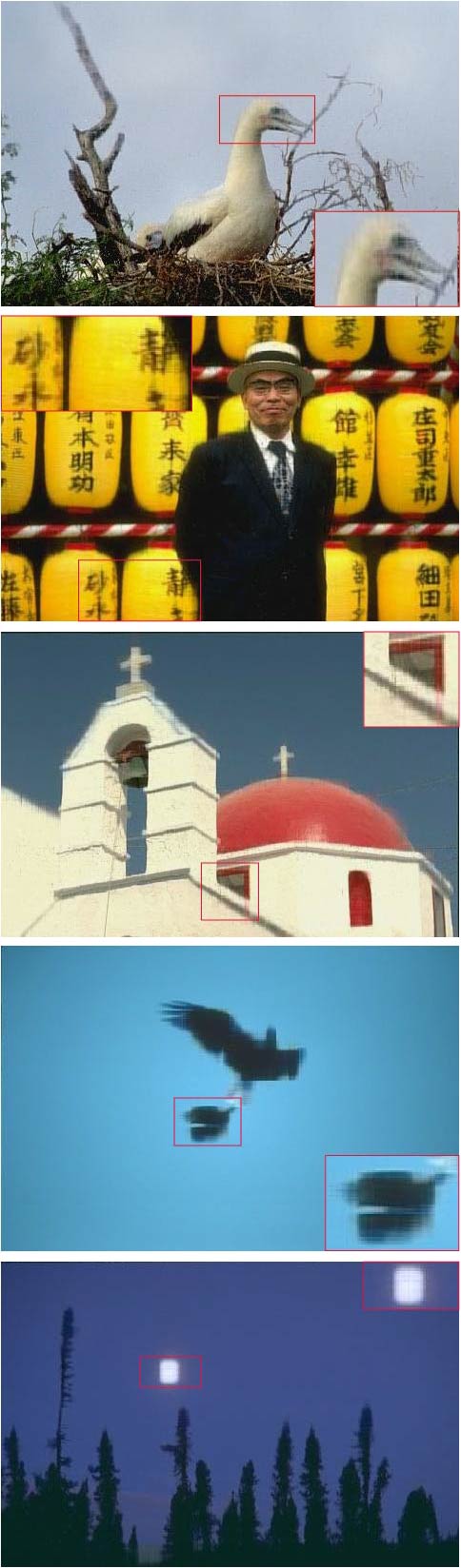
(f) ETRPCA

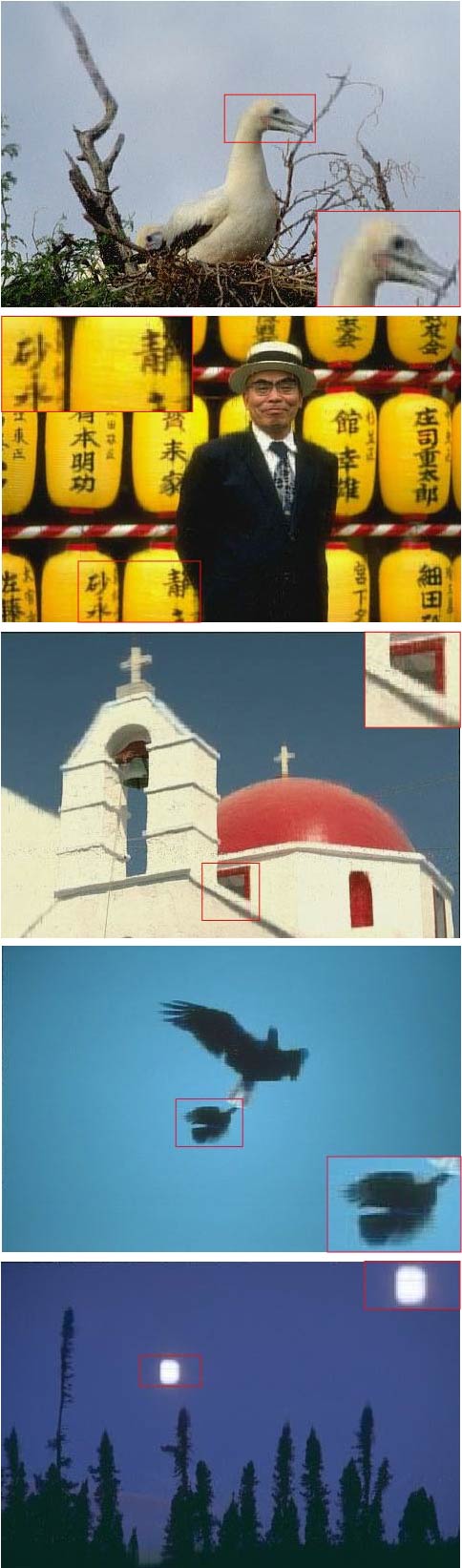
(g) GWTRPCA

Figure 5: Recovery performance comparison of 5 example images on the BSD dataset. (a) Original image; (b) observed image; (c)-(g) recovered images by RPCA, SNN, TRPCA, ETRPCA and our method GWTRPCA, respectively.The PSNR values can be seen in Tab. 2. Best viewed in ×2 sized color pdf file.

Secondly, we test the capability of GWTRPCA to learn adaptive weights by a modified Cauchy estimator. We use GWTRPCA to recover the same image and also set $\mathbf{w}^{intra}=\mathbf{1}$. As is shown in Fig. 4, the performance of our method is most outstanding. Besides, it can be seen that the weight $\mathbf{w}^{inter}$ learned by our method obeys the decreasing property mentioned in Eq. (10) and (11). Hence, GWTRPCA can achiecve better recovery by our adaptive weight learning strategy.

Now we utilize the MCE to calculate the inter-frontal slice weight as follows: It is worth noting that our adaptive weight learning strategy can also be employed to calculate the intra-frontal slice weight $\mathbf{w}^{intra}$.

Index	1	2	3	4	5
RPCA	24.51	23.46	24.08	30.78	29.95
SNN	26.42	25.20	25.40	26.20	28.33
TRPCA	28.28	25.40	27.20	31.73	33.73
ETRPCA	28.49	26.20	27.78	32.41	34.74
GWTRPCA	29.29	27.72	28.96	34.09	36.08

Table 2: Comparison of PSNR values of RPCA, SNN, TRPCA, ETRPCA and GWTRPCA on 5 example images utilized in Fig. 5. The best results are marked bold.

Experiments

In this section, we compare our method GWTRPCA with other competing methods such as RPCA (Candès et al. 2011), SNN (Huang et al. 2015), TRPCA (Lu et al. 2020) and ETRPCA (Gao et al. 2021) on the application of color image recovery and hyperspectral image denoising. We manually set the weight $\mathbf{w}^{intra}$ like ETRPCA. We devide singular values into three groups and corresponding weight is set to 0.8, 0.8 and 1.2. We utilize the Peak Signal-to-Noise Ratio (PSNR) (Wang et al. 2004) to evaluate recovery performance and the higher PSNR value the better recovery.

Application to Color Image Recovery

In this experiment, we apply GWTRPCA for color image recovery. It has been shown color images can be well approximated by low rank matrices or tensors (Liu et al. 2013). We conduct experiments on two real-world datasets: Berkeley Segmentation dataset (BSD) (Arbelaez et al. 2011) and Kodak image dataset (Kodak) (E. Kodak 1999). For each image, we randomly set 10% of pixels to random values in [0,255] and the positions of the corrupted pixels are unknown. All 3 channels of color images are corrupted at the same positions and the corruptions are on the sparse tubes.

We compare our method GWTRPCA with RPCA, SNN, TRPCA and ETRPCA on image recovery. For RPCA, we apply it on each channnel and receive the final recovered image by comnbining the results. We set the parameter $\lambda=1/\sqrt{\max\left(d_{1},d_{2}\right)}$ as suggested in theory (Candès et al. 2011). For SNN, we find that SNN does not perform well when the parameter are set to the values suggested in theory (Huang et al. 2015). Hence, we empirically set $\lambda=[15,15,1.5]$ to ensure SNN can achieve great performance in most cases. For TRPCA, ETRPCA and GWTRPCA, the parameter is all set to $\lambda=1/\sqrt{d_{3}\max\left(d_{1},d_{2}\right)}$.

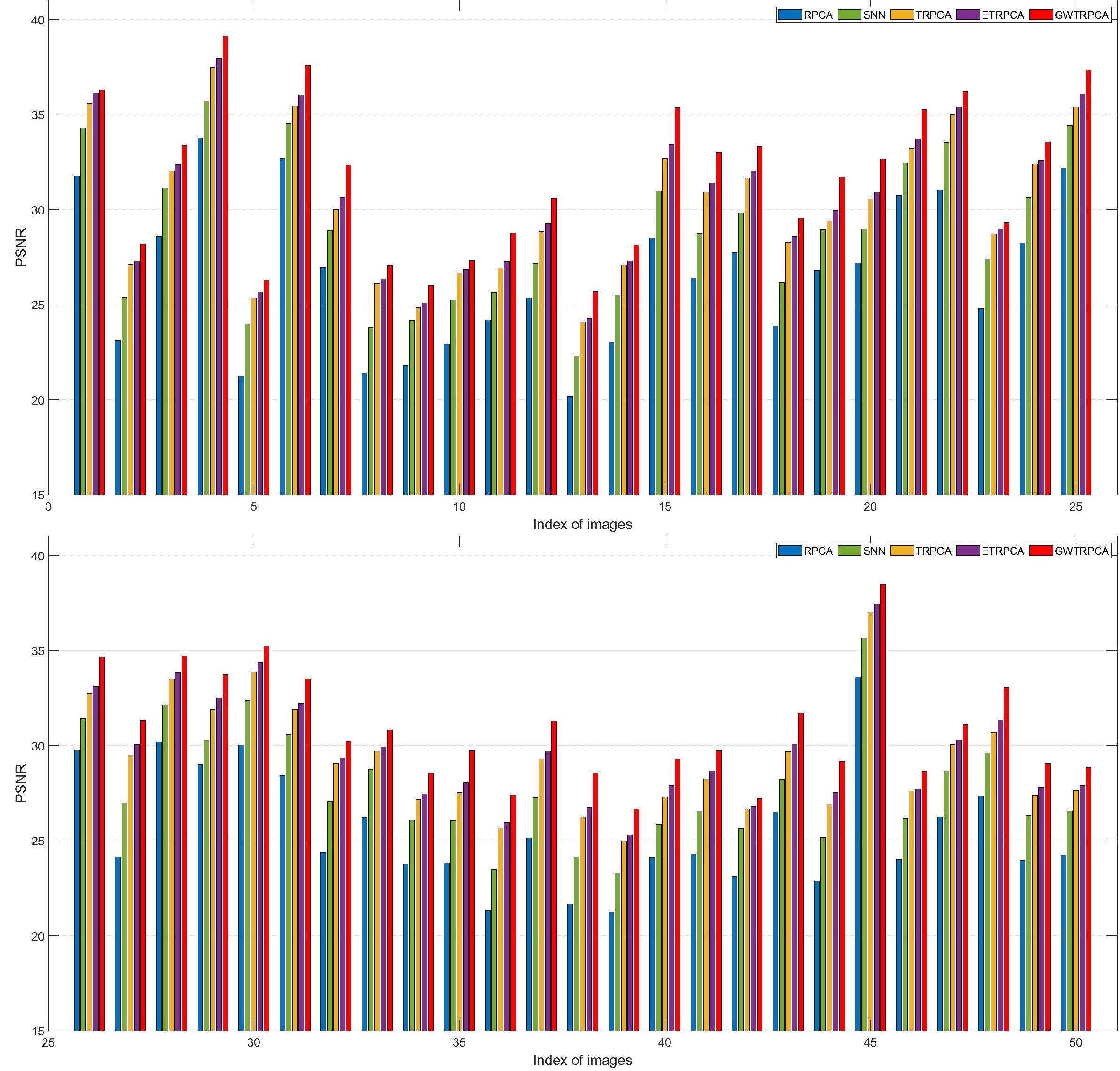
Figure 6: Comparsion of the PSNR values of RPCA, SNN, TRPCA, ETRPCA and our method GWTRPCA for image recovery on 50 images of BSD. Top row: PSNR values of the first 25 images, Bottom row: PSNR values of the remaining 25 images.

Dataset	BSDtrain	BSDval	BSDtest	BSD
RPCA	25.52	25.02	25.10	25.25
SNN	27.63	27.20	27.20	27.37
TRPCA	29.11	28.72	28.63	28.84
ETRPCA	29.50	29.07	29.03	29.22
GWTRPCA	30.71	30.12	30.23	30.40

Table 3: Comparison of average PSNR values of different methods on the BSD dataset and its three subsets. BSDtrain, BSDval, BSDtest and BSD consist of 200, 100, 200 and 500 natural images, respectively. The best results are marked bold.

Some examples of the recovered images on the BSD dataset can be seen in Fig. 5. The PSNR values of several methods on 50 color images of BSD is shown in Fig. 6. Tab. 3 illustrates the PSNR values of GWTRPCA and other comparison methods on the BSD dataset. More reuslts on the Kodak dataset can be seen in Supplementary Material C. From these reuslts, we have the following conclusions. Firstly, tensor based methods (SNN, TRPCA, ETRPCA and GWTRPCA) are generally superior than the matrix based RPCA. The reason is that RPCA applys the image recovery on each channel independently and fails to exploit the high-order information across the channels. On the contrary, tensor based methods can employ the multi-dimensional structure of color image. Secondly, GWTRPCA can recover more edge and color information than TRPCA and ETRPCA. The reason can be that GWTRPCA considers the global information of tensor singular values and can achieve better recovery results. Besdies, ETRPCA only empirically and manually sets the weights to ensure great performance. GWTRPCA can adaptively learn the inter-frontal slice weights.

Noise Level	10%	20%	30%	40%
RPCA	30.30	28.58	26.35	23.42
SNN	33.05	31.46	29.86	28.20
TRPCA	45.84	43.82	40.89	35.63
ETRPCA	45.87	43.90	40.93	37.99
GWTRPCA	46.56	44.51	41.37	38.50

Table 4: Comparison of average PSNR values of different methods on the Washington DC Mall HSI dataset under varying noises for HSI denoising. The best results are marked bold.

Noise Level	10%	20%	30%	40%
RPCA	27.24	26.30	25.27	23.90
SNN	29.07	28.02	26.95	25.86
TRPCA	41.21	39.84	38.40	36.57
ETRPCA	41.24	39.89	38.44	36.66
GWTRPCA	48.73	47.26	45.40	41.78

Table 5: Comparison of average PSNR values of different methods on the Pavia University HSI dataset under varying noises for HSI denoising. The best results are marked bold.

Application to Hyperspectral Image Denoising

In this part, we verify the effectiveness of GWTRPCA on hyperspectral image (HSI) denoising. We conduct experiments on the Washington DC Mall and Pavia University HSI datasets, which can be treated as a tensor of size $256\times 256\times 150$ and $610\times 340\times 103$, respectively.

We add random salt-pepper noise to each hyperspectral image and the noise level is set from 10% to 40%. The average PSNR values of HSI denoising of GWTRPCA and other competitors are reported in Tab. 4 and Tab. 5. It’s easy to see that GWTRPCA outperforms other methods. The denoising results can be worse with the increase of noise level. Despite this, our method earns more outstanding results even when the noise level is set to 40%.

Conclusion

In this paper, we propose the Global Weighted Tensor Robust Principal Component Analysis (GWTRPCA) method based on a new defined Global Weighted Tensor Nuclear Norm (GWTNN). We simultaneously consider the importance of intra-frontal slice and inter-frontal slice singular values. With the aid of global information of singular values, GWTRPCA can approximate the tubal rank function more exactly. Furthermore, we utilize a MCE to adaptively learn inter-frontal slice weights. An effective algorithm is devised to solve the GWTRPCA optimization problem based on the ADMM framework. Finally, the experiments on real-world databases validate the effectiveness of the proposed method.

References

- Arbelaez et al. (2011) Arbelaez, P.; Maire, M.; Fowlkes, C.; and Malik, J. 2011. Contour Detection and Hierarchical Image Segmentation. IEEE Transactions on Pattern Analysis and Machine Intelligence, 33(5): 898–916.
- Bouwmans et al. (2018) Bouwmans, T.; Javed, S.; Zhang, H.; Lin, Z.; and Otazo, R. 2018. On the applications of robust PCA in image and video processing. Proceedings of the IEEE, 106(8): 1427–1457.
- Cai et al. (2019) Cai, S.; Luo, Q.; Yang, M.; Li, W.; and Xiao, M. 2019. Tensor robust principal component analysis via non-convex low rank approximation. Applied Sciences, 9(7): 1411.
- Candès et al. (2011) Candès, E.; Li, X.; Ma, Y.; and Wright, J. 2011. Robust principal component analysis? Journal of the ACM, 58(3): 1–37.
- E. Kodak (1999) E. Kodak. 1999. Kodak lossless true color image suite (PhotoCD PCD0992). http://r0k.us/graphics/kodak. Accessed: 1999-11-15.
- Gao et al. (2020) Gao, Q.; Xia, W.; Wan, Z.; Xie, D.; and Zhang, P. 2020. Tensor-SVD based graph learning for multi-view subspace clustering. In Proceedings of the AAAI Conference on Artificial Intelligence (AAAI), 3930–3937.
- Gao et al. (2021) Gao, Q.; Zhang, P.; Xia, W.; Xie, D.; Gao, X.; and Tao, D. 2021. Enhanced Tensor RPCA and its Application. IEEE Transactions on Pattern Analysis and Machine Intelligence, 43(6): 2133–2140.
- Gu et al. (2017) Gu, S.; Xie, Q.; Meng, D.; Zuo, W.; Feng, X.; and Zhang, L. 2017. Weighted nuclear norm minimization and its applications to low level vision. International Journal of Computer Vision, 121(2): 183–208.
- Huang et al. (2015) Huang, B.; Mu, C.; Goldfarb, D.; and Wright, J. 2015. Provable models for robust low-rank tensor completion. Pacific Journal of Optimization, 11(2): 339–364.
- Huber (1981) Huber, P. J. 1981. Robust Statistics. New York: Wiley.
- Jiang et al. (2020) Jiang, T.; Huang, T.; Zhao, X.; and Deng, L. 2020. Multi-dimensional imaging data recovery via minimizing the partial sum of tubal nuclear norm. Journal of Computational and Applied Mathematics, 372: 112680.
- Kilmer and Martin (2011) Kilmer, M.; and Martin, C. 2011. Factorization strategies for third-order tensors. Linear Algebra and its Applications, 435(3): 641–658.
- Kolda and Bader (2009) Kolda, T. G.; and Bader, B. W. 2009. Tensor decompositions and applications. SIAM review, 51(3): 455–500.
- Kong, Xie, and Lin (2018) Kong, H.; Xie, X.; and Lin, Z. 2018. t-Schatten- norm for low-rank tensor recovery. IEEE Journal of Selected Topics in Signal Processing, 12(6): 1405–1419.
- Koren (2008) Koren, Y. 2008. Factorization meets the neighborhood: a multifaceted collaborative filtering model. In Proceedings of the 14th ACM SIGKDD international conference on Knowledge discovery and data mining (KDD), 426–434.
- Li and Ma (2021) Li, T.; and Ma, J. 2021. T-SVD based non-convex tensor completion and robust principal component analysis. In International Conference on Pattern Recognition (ICPR), 6980–6987.
- Liu et al. (2013) Liu, J.; Musialski, P.; Wonka, P.; and Ye, J. 2013. Tensor completion for estimating missing values in visual data. IEEE Transactions on Pattern Analysis and Machine Intelligence, 35(1): 208–220.
- Liu, Chen, and Zhu (2018) Liu, Y.; Chen, L.; and Zhu, C. 2018. Improved Robust Tensor Principal Component Analysis via Low-Rank Core Matrix. IEEE Journal of Selected Topics in Signal Processing, 12(6): 1378–1389.
- Lu et al. (2020) Lu, C.; Feng, J.; Chen, Y.; Liu, W.; Lin, Z.; and Yan, S. 2020. Tensor Robust Principal Component Analysis with a New Tensor Nuclear Norm. IEEE Transactions on Pattern Analysis and Machine Intelligence, 42(4): 925–938.
- Mu et al. (2020) Mu, Y.; Wang, P.; Lu, L.; Zhang, X.; and Qi, L. 2020. Weighted tensor nuclear norm minimization for tensor completion using tensor-SVD. Pattern Recognition Letters, 130: 4–11.
- Pang et al. (2020) Pang, M.; Cheung, Y.-M.; Wang, B.; and Lou, J. 2020. Synergistic Generic Learning for Face Recognition From a Contaminated Single Sample per Person. IEEE Transactions on Information Forensics and Security, 15: 195–209.
- Wang et al. (2020) Wang, S.; Liu, Y.; Feng, L.; and Zhu, C. 2020. Frequency-Weighted Robust Tensor Principal Component Analysis. arXiv:2004.10068.
- Wang et al. (2004) Wang, Z.; Bovik, A.; Sheikh, H.; and Simoncelli, E. 2004. Image quality assessment: from error visibility to structural similarity. IEEE Transactions on Image Processing, 13(4): 600–612.