Backward Reachability Analysis of Neural Feedback Loops: Techniques for Linear and Nonlinear Systems

Abstract

As neural networks (NNs) become more prevalent in safety-critical applications such as control of vehicles, there is a growing need to certify that systems with NN components are safe. This paper presents a set of backward reachability approaches for safety certification of neural feedback loops (NFLs), i.e., closed-loop systems with NN control policies. While backward reachability strategies have been developed for systems without NN components, the nonlinearities in NN activation functions and general noninvertibility of NN weight matrices make backward reachability for NFLs a challenging problem. To avoid the difficulties associated with propagating sets backward through NNs, we introduce a framework that leverages standard forward NN analysis tools to efficiently find over-approximations to backprojection (BP) sets, i.e., sets of states for which an NN policy will lead a system to a given target set. We present frameworks for calculating BP over-approximations for both linear and nonlinear systems with control policies represented by feedforward NNs and propose computationally efficient strategies. We use numerical results from a variety of models to showcase the proposed algorithms, including a demonstration of safety certification for a 6D system.

Reachability, Neural Networks, Safety, Neural Feedback Loops, Linear Systems, Nonlinear Systems

1 Introduction

Neural network-based control has seen success in domains that remain difficult for more classical control methods, such as robotic locomotion over varied terrain [1, 2], recovery of a quadrotor from aggressive maneuvers [3], and robotic manipulation [4, 5]. Neural network-based control also offers complementary properties compared to classical linear control and more recent optimal control approaches [6, 7]. Neural network-based control is capable of handling complex nonlinear systems, and like linear control it can be fast to execute. However, the standard training procedures for NN-based control do not provide the convergence and safety guarantees that can usually be derived for more classical control approaches. Further, despite achieving high performance during testing, many works have demonstrated that NNs can be sensitive to small perturbations in the input space and produce unexpected behavior or incorrect conclusions as a result [8, 9]. Thus, before applying NNs to safety-critical systems such as self-driving cars [10, 11, 12] and aircraft collision avoidance systems [13], there is a need for tools that provide safety guarantees. Providing safety guarantees presents computational challenges due to the high dimensional and nonlinear nature of NNs.

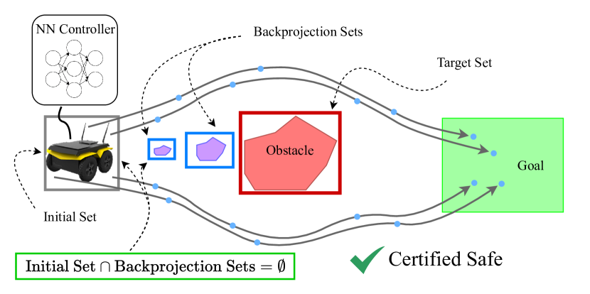
(a) Backward reachability for collision avoidance: BP set estimates (blue) approximate the set of states that lead to the obstacle (red), thus if the initial state set does not intersect with any BPs, the situation is safe.

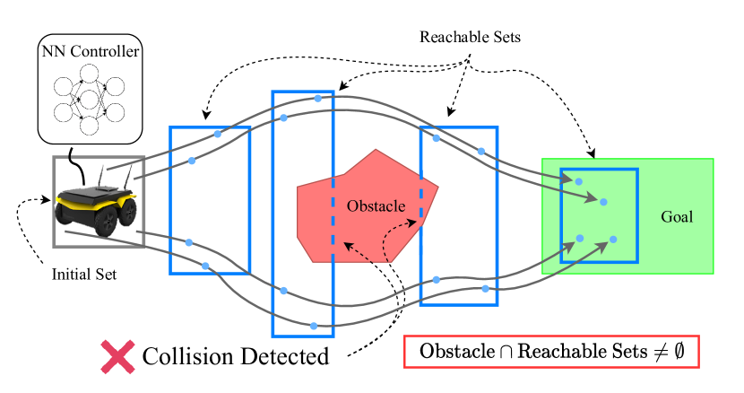
(b) Forward reachability for collision avoidance: forward reachable set estimates (blue) approximate the set of possible future states of the system, thus any intersection with an obstacle means safety cannot be certified.

Figure 1: Collision avoidance scenario. Backward reachability correctly guarantees safety whereas forward reachability fails.

There is a growing body of work focused on synthesizing NN controllers with safety and performance guarantees [14, 15, 16, 17, 18, 19], but this does not preclude the need for verification and safety analysis after synthesis. To this end, many open-loop NN analysis tools [20, 21, 22, 23, 24, 25, 26, 27, 28] have been developed to make statements about possible NN outputs given a set of inputs. To extend analysis techniques to closed-loop systems with NN controllers, i.e., neural feedback loops (NFLs), there has also been effort towards developing reachability analysis techniques [28, 29, 30, 31, 32, 33, 34, 35, 36, 37, 38] that determine how a system’s state evolves over time. While forward reachability [28, 29, 30, 31, 32, 33, 34, 35, 36, 37] certifies safety by checking that possible future states of the system do not enter dangerous regions, this paper focuses on backward reachability [38], wherein safety is certified by checking that the system does not start from a state that could lead to a dangerous region, as shown in Fig. 1(a). Thus, the challenge of backward reachability analysis is to calculate backprojection (BP) sets that define regions of the state space for which the NN control policy will drive the system into a given target set, which can be chosen to contain a dangerous part of the state space.

Contrasting Fig. 1(a) with Fig. 1(b) shows how backward reachability can be less conservative than forward reachability in scenarios where there are multiple modes for possible trajectories branching from a given initial state set. In Fig. 1(b), the robot’s position within the initial state set determines whether it will go above or below the obstacle. The forward reachable sets must contain all possible future trajectories, so when the forward reachable sets are represented by single convex sets (as is the case in [29, 30, 31, 32, 33, 34, 35, 36]), they must span the upper and lower trajectories, thus detecting a possible collision with the obstacle and failing to certify safety. Alternatively, because the BP sets in Fig. 1(a) do not intersect with the initial state set, the robot is not among the states that leads to an obstacle, allowing backward reachability to certify safety.

For systems without NNs, switching between forward and backward reachability analysis is relatively simple [39, 40, 41]. However, nonlinear activation functions and noninvertible weight matrices common to NNs make it challenging to determine a set of inputs given a set of outputs. While recent work [28, 38, 36] has made advances in backward reachability of NFLs, there are no existing techniques that efficiently find BP set estimates over multiple timesteps for linear and nonlinear systems with feedforward NNs that give continuous outputs. Thus, our contributions include:

• A set of algorithms that enable computationally efficient safety certification of linear and nonlinear NFLs by calculating over-approximations of BP sets.

• Validation of our methods using numerical experiments for control-relevant applications including obstacle avoidance for mobile robots and quadrotors.

This work extends prior work [42] by introducing:

• HyBReach-LP: A hybrid of the two previously proposed algorithms [42] that improves the tradeoff between conservativeness and computation time.

• A guided partitioning algorithm that reduces conservativeness faster than uniform partitioning strategies.

• BReach-MILP: an algorithm to compute BP sets for systems with nonlinear dynamics using techniques developed by [35].

• Numerical experiments that exhibit our BP estimation techniques on higher-order and nonlinear systems, including an ablation study marking improvements from [42].

2 Related Work

This section describes how reachability analysis can be applied to three categories of systems: NNs in isolation (i.e., open-loop analysis), closed-loop systems without neural components, and NFLs.

Open-loop NN analysis refers to methods that determine a relation between sets of inputs to an NN and sets of the NN’s output. Open-loop NN analysis encompasses techniques that relax the nonlinearities in the NN activation functions to quickly provide relatively conservative bounds on NN outputs [20, 23], and techniques that take more time to provide exact bounds [26, 28]. Often, these tools are motivated by the threat posed by adversarial attacks [23, 24] that can drastically affect the output of perception models. To extend the use of open-loop analysis tools to NFLs, the closed-loop system dynamics must be considered.

Reachability analysis is a well-established method for safety verification of closed-loop systems without NN components. Hamilton-Jacobi methods [39, 40] provide the main theoretical framework for these analyses, and computational tools such as CORA [43], Flow* [44], SpaceEx [45], HYLAA [46], and C2E2 [47] can be used to compute reachable sets for a given system. However, these tools cannot currently be used to analyze NFLs.

When it comes to NFLs, forward reachability analysis is the focus of recent work [28, 29, 30, 31, 32, 33, 34, 35, 36, 37]. Unlike traditional reachability analysis techniques such as Hamilton-Jacobi methods [39, 40], backward reachability analysis of NFLs introduces significant challenges that are not present in forward reachability of NFLs. Forward reachability of NFLs relies on open-loop NN analysis tools that are configured to pass sets forward through an NN. This suggests that backward reachability would need a way to propagate sets backward through an NN, but this presents two major challenges: First, many activation functions do not have a one-to-one mapping of inputs to outputs (consider $\mathrm{ReLU}(x)=0$, which corresponds to any value $x\leq 0$). In these cases, propagating sets backward through an NN can cause an infinitely large BP sets. Additionally, the weight matrices in each layer of the NN may be singular or rank deficient, meaning they are not generally invertible, which presents another fundamental challenge in determining a set of inputs from a set of outputs.

While recent works on NN inversion have developed NN architectures that are designed to be invertible [48] and training procedures that regularize for invertibility [49], dependence on these techniques would be a major limitation on the class of systems for which backward reachability analysis could be applied. Our approach avoids the challenges associated with NN-invertibility. For linear systems, our approach can be applied to the same class of NN architectures as CROWN [20], i.e., NNs for which an affine relaxation can be found. For nonlinear systems, our approach can be applied to any NN with piecewise-linear activation functions (ReLU, Leaky ReLU, hardtanh, etc.).

Recent work investigated backwards reachability analysis for NFLs. vincent2021reachable describe a method for backward reachability on an NN dynamics model, but this method is limited to NNs with ReLU activations. Alternatively, [38] use a quantized state approach [27] to quickly compute BP sets, but it requires an alteration of the original NN through a preprocessing step that can affect its overall behavior and does not consider continuous NN outputs. Finally, [36] derive a closed-form equation that can be used to find BP set under-approximations, but under-approximations cannot be used to guarantee safety because they may miss some states that reach the target set (under-approximations are most useful for goal checking, where it is desirable to guarantee that all states in the BP estimate reach the target set). This work expands upon the existing literature on backward reachability for NFLs by introducing a framework for efficiently calculating BP set over-approximations for NFLs with continuous action spaces.

3 Preliminaries

3.1 System Dynamics

We consider a discrete-time time-invariant system with dynamics given by

$$\mathbf{x}_{t+1}=p(\mathbf{x}_{t},\mathbf{u}_{t}),$$ (1)

where $\mathbf{x}_{t}\in\mathds{R}^{n_{x}}$ is the state, $n_{x}$ is the state dimension, $\mathbf{u}_{t}\in\mathds{R}^{n_{u}}$ is the control input, and $n_{u}$ is the control dimension. In the linear case, Eq. 1 may be written

$$\mathbf{x}_{t+1}=\mathbf{A}\mathbf{x}_{t}+\mathbf{B}\mathbf{u}_{t}+\mathbf{c}.$$ (2)

The matrices $\mathbf{A}$, $\mathbf{B}$, and $\mathbf{c}$ are assumed known. In both linear and nonlinear cases, the control input $\mathbf{u}_{t}$ is generated by a state-feedback control policy specified by an $m$-layer feedforward NN $\pi(\cdot)$, i.e., $\mathbf{u}_{t}=\pi(\mathbf{x}_{t})$. The closed-loop system Eq. 1 with control policy $\pi$ is denoted

$$\mathbf{x}_{t+1}=f(\mathbf{x}_{t};\pi).$$ (3)

We assume $\mathbf{u}_{t}$ is constrained by control limits and is thus limited to a convex set of allowable control values $\mathcal{U}$, i.e., $\mathbf{u}_{t}\in\mathcal{U}$. Similarly, we consider $\mathbf{x}_{t}$ to be constrained to a convex operating region of the state space $\mathcal{X}$, i.e., $\mathbf{x}_{t}\in\mathcal{X}$. Note that for nonlinear systems, $\mathcal{X}$ represents the set of states that are physically realizable for a given system, e.g., the maximum speed of a vehicle that cannot be exceeded regardless of input. We implement this by using clipping in the dynamics. However, for linear systems, we do not clip, as this would introduce non-linearity. Defining $\mathcal{X}$ is particularly important for backward reachability, because the target set says nothing about initial states that are practical. For example, a very high velocity could cause the positional range of the backprojection set to also be quite large, but the practitioner might know that the system would never start from a set of states that allow for such a high velocity to be achieved in the time horizon. To encode this idea in the optimization problems, we assume $\mathcal{X}$ is given and contains all possible previous states.

3.2 Nonlinear System Over-Approximation

We calculate backreachable and backprojection sets for nonlinear systems by extending the mixed integer linear programming (MILP) methods of [35], which over-approximate nonlinear dynamics using piecewise-linear representations. Using a piecewise-linear over-approximation of the nonlinear dynamics preserves the ability to calculate global optima for the optimization problem as well as make sound claims about the original nonlinear system. As described by [35], the closed-loop system dynamics function Eq. 1 mapping $\mathbb{R}^{n_{x}}\rightarrow\mathbb{R}^{n_{x}}$ is considered as $n_{x}$ functions mapping $\mathbb{R}^{n_{x}}\rightarrow\mathbb{R}$. Each function mapping $\mathbb{R}^{n_{x}}\rightarrow\mathbb{R}$ is re-written into a series of affine functions and $\mathbb{R}\rightarrow\mathbb{R}$ nonlinear functions. For each nonlinear function $e(x)$ defined over the interval $x\in[a,b]$, an optimally-tight piecewise-linear upper and lower bound is computed such that: $g_{e_{LB}}(x)\leq e(x)\leq g_{e_{UB}}(x)~{}~{}\forall x\in[a,b]$. Together, the affine functions and piecewise-linear lower and upper bounds form an abstraction $\hat{p}$ of the original nonlinear closed-loop system $p$ Eq. 1. With control policy $\mathbf{u}_{t}=\pi(\mathbf{x}_{t})$, we denote the abstract closed-loop system relating $\mathbf{x}_{t}$ and $\mathbf{x}_{t+1}$ as $\hat{f}(\mathbf{x}_{t};\pi)$. The abstract closed-loop system represents an over-approximation of $f(\cdot)$, or more formally $\forall\mathbf{x}_{t}\in\mathcal{X}$,

$$\{\mathbf{x}_{t+1}\lvert\ \mathbf{x}_{t+1}=f(\mathbf{x}_{t};\pi)\}\subseteq\{\mathbf{x}_{t+1}\lvert\ \mathbf{x}_{t+1}\bowtie\hat{f}(\mathbf{x}_{t};\pi)\}$$ (4)

where we denote that a state $\mathbf{x}_{t+1}$ is a valid successor of state $\mathbf{x}_{t}$ under the abstract system if $\mathbf{x}_{t+1}\bowtie\hat{f}(\mathbf{x}_{t};\pi)$.

3.3 Control Policy Neural Network Structure

Consider a feedforward NN with $M$ hidden layers, and one input and one output layer. We denote the number of neurons in each layer as $n_{m},\ \forall m\in[M+1]$ where $[i]$ denotes the set $\{0,1,\ldots,i\}$. The $m$-th layer has weight matrix $\mathbf{W}^{m}\in\mathds{R}^{n_{m+1}\times n_{m}}$, bias vector $\mathbf{b}^{m}\in\mathds{R}^{n_{m+1}}$, and activation function $\sigma^{m}:\mathds{R}^{n_{m+1}}\to\mathds{R}^{n_{m+1}}$. For linear systems, $\sigma^{m}$ can be any option handled by CROWN [20], e.g., sigmoid, tanh, ReLU, and for nonlinear systems $\sigma^{m}$ can be any piecewise-linear function, e.g. ReLU, Leaky ReLU, hardtanh, etc. For an input $\mathbf{x}\in\mathds{R}^{n_{0}}$, the NN output $\pi(\mathbf{x})$ is computed as

$$\begin{split}\mathbf{x}^{0}&=\mathbf{x}\\ \mathbf{x}^{m+1}&=\sigma^{m}(\mathbf{W}^{m}\mathbf{x}^{m}+\mathbf{b}^{m}),\forall m\in[M-1]\\ \pi(\mathbf{x})&=\mathbf{W}^{M}\mathbf{x}^{M}+\mathbf{b}^{M}.\end{split}$$ (5)

3.4 Neural Network Relaxation

For linear dynamics, we relax the NN’s activation functions to obtain affine bounds on the NN outputs for a known set of inputs. This preserves the problem as an LP and reduces computational cost. The range of inputs are represented using the $\ell_{p}$-ball

$$\mathcal{B}_{p}(\mathring{\mathbf{x}},\bm{\epsilon)} \triangleq\{\mathbf{x}\ \lvert\ \|(\mathbf{x}-\mathring{\mathbf{x}})\oslash\bm{\epsilon}\|_{p}\leq 1\},$$ (6)

where $\mathring{\mathbf{x}}\in\mathds{R}^{n}$ is the center of the ball, $\bm{\epsilon}\in\mathds{R}^{n}_{\geq 0}$ is a vector whose elements are the radii for the corresponding elements of $\mathbf{x}$, and $\oslash$ denotes element-wise division.

Theorem 3.1 (​​[20], Convex Relaxation of NN)

Given an $m$-layer neural network control policy $\pi:\mathds{R}^{n_{x}}\to\mathds{R}^{n_{u}}$, there exist two explicit functions $\pi_{j}^{L}:\mathds{R}^{n_{x}}\to\mathds{R}^{n_{u}}$ and $\pi_{j}^{U}:\mathds{R}^{n_{x}}\to\mathds{R}^{n_{u}}$ such that $\forall j\in[n_{m}],\forall\mathbf{x}\in\mathcal{B}_{p}(\mathring{\mathbf{x}},\bm{\epsilon)}$, the inequality $\pi_{j}^{L}(\mathbf{x})\leq\pi_{j}(\mathbf{x})\leq\pi_{j}^{U}(\mathbf{x})$ holds true, where

$$\pi_{j}^{U}(\mathbf{x})=\mathbf{\Psi}_{j,:}\mathbf{x}+\bm{\alpha}_{j},\quad\pi_{j}^{L}(\mathbf{x})=\mathbf{\Phi}_{j,:}\mathbf{x}+\bm{\beta}_{j},$$ (7)

where $\mathbf{\Psi},\mathbf{\Phi}\in\mathds{R}^{n_{u}\times n_{x}}$ and $\bm{\alpha},\bm{\beta}\in\mathds{R}^{n_{u}}$ are defined recursively using NN weights, biases, and activations (e.g., ReLU, sigmoid, tanh) [20].

3.5 Backreachable & Backprojection Sets

Figure 2: Target, backreachable, and backprojection sets/over-approximations. Given a target set, $\mathcal{X}_{T}$, the backreachable set $\mathcal{R}_{-1}(\mathcal{X}_{T})$ contains all states where some control exists such that the system goes to $\mathcal{X}_{T}$ in one timestep. The BP set $\mathcal{P}_{-1}(\mathcal{X}_{T})$ contains all states for which the NN controller leads the system to $\mathcal{X}_{T}$. Backreachable overapproximation $\bar{\mathcal{R}}_{-1}(\mathcal{X}_{T})$ contains states for which some control exists to move the system to $\mathcal{X}_{T}$ under the relaxed dynamics. BP under-approximation $\underaccent{\bar}{\mathcal{P}}_{-1}(\mathcal{X}_{T})$ and over-approximation $\bar{\mathcal{P}}_{-1}(\mathcal{X}_{T})$ contain states for which all and some, respectively, successor states under the relaxed system (controller, dynamics, or both) lead the system to $\mathcal{X}_{T}$.

Given a target set $\mathcal{X}_{T}$ as shown on the right side of Fig. 2, each of the five sets on the left contain states that will reach $\mathcal{X}_{T}$ under different conditions as described below. First, the one-step backreachable set

$$\mathcal{R}_{-1}(\mathcal{X}_{T})\triangleq\{\mathbf{x}_{t}\ \in\mathcal{X}\lvert\ \exists\mathbf{u}_{t}\in\mathcal{U}\mathrm{\ s.t.\ }p(\mathbf{x}_{t},\mathbf{u}_{t})\in\mathcal{X}_{T}\},$$ (8)

contains the set of all states that transition to $\mathcal{X}_{T}$ in one timestep given some $\mathbf{u}_{t}\in\mathcal{U}$. However, in the nonlinear case, the backreachable set cannot be computed exactly. The dynamics $p$ are abstracted using an over-approximation and as a consequence we compute an over-approximation of the backreachable set

$$\bar{\mathcal{R}}_{-1}(\mathcal{X}_{T})\triangleq \{\mathbf{x}_{t}\ \in\mathcal{X}\lvert\ \exists\mathbf{u}_{t}\in\mathcal{U},~{}\exists\mathbf{x}_{t+1}\bowtie\hat{p}(\mathbf{x}_{t},\mathbf{u}_{t})\mathrm{\ s.t.\ }$$

$$~{}~{}\mathbf{x}_{t+1}\in\mathcal{X}_{T}\}$$ (9)

where a state $\mathbf{x}_{t+1}$ is a valid successor of $\mathbf{x}_{t}$ for some $\mathbf{u}_{t}\in\mathcal{U}$ under the abstract system $\hat{p}$ if $\mathbf{x}_{t+1}\bowtie\hat{p}(\mathbf{x}_{t},\mathbf{u}_{t})$.

The importance of the backreachable set is that it only depends on the control limits $\mathcal{U}$ and not the NN control policy $\pi$. Thus, while $\mathcal{R}_{-1}(\mathcal{X}_{T})$ is itself a very conservative over-approximation of the true set of states that will reach $\mathcal{X}_{T}$ under $\pi$, for the linear case it provides a region over which we can relax the NN with forward NN analysis tools, and in the nonlinear case, a less conservative region over which to approximate the dynamics and encode the NN.

Next, we define the one-step true BP set as

$$\mathcal{P}_{-1}(\mathcal{X}_{T})\triangleq\{\mathbf{x}_{t}\ \lvert\ f(\mathbf{x}_{t};\pi)\in\mathcal{X}_{T}\},$$ (10)

which denotes the set of all states that will reach $\mathcal{X}_{T}$ in one timestep given a control input from $\pi$. As previously noted, calculating $\mathcal{P}_{-1}(\mathcal{X}_{T})$ exactly is computationally intractable for both linear and nonlinear systems due to the presence of the NN control policy, which motivates the development of approximation techniques. Thus, the final two sets shown in Fig. 2 are the BP set over-approximation and BP set under-approximation.

In the linear case, the NN control policy $\pi$ is abstracted and in the nonlinear case the dynamics $p$ are abstracted. We generalize by denoting the abstract system $\hat{f}$ in both cases. The BP set over-approximation can then be written

$$\bar{\mathcal{P}}_{-1}(\mathcal{X}_{T}) \triangleq\{\mathbf{x}_{t}\ \lvert\ \exists\mathbf{x}_{t+1}\bowtie\hat{f}(\mathbf{x}_{t};\pi)\mathrm{\ s.t.\ }$$ (11)

$$\mathbf{x}_{t+1}\in\mathcal{X}_{T}\},\$$

and the BP set under-approximation can then be written

$$\underaccent{\bar}{\mathcal{P}}_{-1}(\mathcal{X}_{T}) \triangleq\{\mathbf{x}_{t}\ \lvert\ \forall\mathbf{x}_{t+1}\bowtie\hat{f}(\mathbf{x}_{t};\pi)\mathrm{\ s.t.\ }$$ (12)

$$\mathbf{x}_{t+1}\in\mathcal{X}_{T}\}.\$$

In the linear case the BP set over-approximation can be written more explicitly as

$$\bar{\mathcal{P}}_{-1}(\mathcal{X}_{T}) \triangleq\{\mathbf{x}\ \lvert\ \exists\mathbf{u}\in[\pi^{L}(\mathbf{x}),\pi^{U}(\mathbf{x})]\mathrm{\ s.t.\ }$$ (13)

$$\mathbf{A}\mathbf{x}+\mathbf{B}\mathbf{u}+\mathbf{c}\in\mathcal{X}_{T}\},\$$

and the BP set under-approximation as

$$\underaccent{\bar}{\mathcal{P}}_{-1}(\mathcal{X}_{T}) \triangleq\{\mathbf{x}\ \lvert\ \forall\mathbf{u}\in[\pi^{L}(\mathbf{x}),\pi^{U}(\mathbf{x})]\mathrm{\ s.t.\ }$$ (14)

$$\mathbf{A}\mathbf{x}+\mathbf{B}\mathbf{u}+\mathbf{c}\in\mathcal{X}_{T}\}.\$$

Comparison of the motivation behind over- and under-approximation strategies is given in the next section. From here we will omit the argument $\mathcal{X}_{T}$ from our notation, i.e., $\bar{\mathcal{P}}_{t}\triangleq\bar{\mathcal{P}}_{t}(\mathcal{X}_{T})$, except where necessary for clarity.

3.6 Backprojection Set: Over- vs. Under-Approximations

Given the need to approximate BP sets, it is natural to question whether it is necessary to over- or under-approximate the BP sets. The “for all” condition (i.e., $\forall\mathbf{u}\in[\pi^{L}(\mathbf{x}),\pi^{U}(\mathbf{x})]$) in Eq. 14 means that BP under-approximations can be used to provide a guarantee that a state will reach the target set since all states within the under-approximation reach the target set. Thus, BP under-approximations are useful to check if a set of states is guaranteed to go to a goal set. Alternatively, the “exists” condition (i.e., $\exists\mathbf{u}\in[\pi^{L}(\mathbf{x}),\pi^{U}(\mathbf{x})]$) in Eq. 13 means that BP over-approximations can be used to check if it is possible for a state to reach the target set. Thus, BP over-approximations are useful to check if a set of states is guaranteed to go to an obstacle/avoid set as we consider in this paper. Note that in this work we use “over-approximation” and “outer-bound” interchangeably.

4 Approach

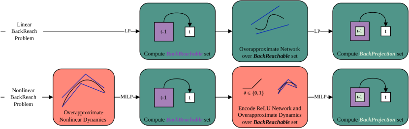
Figure 3: A summary of our approach for computing backprojection sets for both linear and nonlinear dynamical systems.

This section outlines techniques to find multi-step BP set over-approximations $\bar{\mathcal{P}}_{-1}$ for a target set $\mathcal{X}_{T}$. The key insights of computing over-approximate BP sets are captured by first discussing one-step back-projections, and then we explain the extension to multi-step BP set computation. The general procedures for computing one-step BP sets for linear and nonlinear systems are similar and are depicted in Fig. 3 as well as explained in more detail as follows:

1. For smooth nonlinear dynamical systems, construct a piecewise-linear over-approximation of the dynamics, $\hat{p}$, over the operating domain $\mathcal{X}$. For a linear system, $\hat{p}=p$.

2. Ignoring the NN and using control limits $\mathcal{U}$ and state limits $\mathcal{X}$, find the hyper-rectangular bounds $\bar{\mathcal{R}}_{-1}$ on the true backreachable set $\mathcal{R}_{-1}$ (note that $\mathcal{P}_{-1}\subseteq\mathcal{R}_{-1}\subseteq\tilde{\mathcal{R}}_{-1}\subseteq\bar{\mathcal{R}}_{-1}$) by setting up an optimization problem with the following constraints

   $$\mathcal{F}_{\bar{\mathcal{R}}_{-1}}\triangleq\left\{\mathbf{x}_{t},\mathbf{u}_{t}\ \left|\ \begin{aligned} &\mathbf{x}_{t+1}\bowtie\hat{p}(\mathbf{x}_{t},\mathbf{u}_{t}),\\ &\mathbf{x}_{t+1}\in\mathcal{X}_{T},\\ &\mathbf{u}_{t}\in\mathcal{U},\\ &\mathbf{x}_{t}\in\mathcal{X},\\ \end{aligned}\right.\kern-1.2pt\right\},$$ (15)

   and solve

   $$\bar{\bar{\mathbf{x}}}_{t;k}=\min_{\mathbf{x}_{t},\mathbf{u}_{t}\in\mathcal{F}_{\bar{\mathcal{R}}_{-1}}}\mathbf{e}_{k}^{\top}\mathbf{x}_{t},\quad\quad\underaccent{\bar}{\ubar{\mathbf{x}}}_{t;k}=\max_{\mathbf{x}_{t},\mathbf{u}_{t}\in\mathcal{F}_{\bar{\mathcal{R}}_{-1}}}\mathbf{e}_{k}^{\top}\mathbf{x}_{t},$$ (16)

   for each state $k\in[n_{x}]$, where the notation $\mathbf{x}_{t;k}$ denotes the $k^{\mathrm{th}}$ element of $\mathbf{x}_{t}$ and $\mathbf{e}_{k}\ \in\mathds{R}^{n_{x}}$ denotes the indicator vector, i.e., the vector with the $k^{\mathrm{th}}$ element equal to one and all other elements equal to zero. Eq. Equation 16 provides a hyper-rectangular outer bound ${\bar{\mathcal{R}}_{-1}}\triangleq\{\mathbf{x}\ |\ \underaccent{\bar}{\ubar{\mathbf{x}}}_{t}\leq\mathbf{x}\leq\bar{\bar{\mathbf{x}}}_{t}\}$ on the backreachable set.

3. Encode the neural network over the domain of the over-approximation of the backreachable set $\bar{\mathcal{R}}_{-1}$ to obtain contraints corresponding to $\hat{f}(\mathbf{x}_{t};\pi)$. For more detail on the differences in this step between linear and nonlinear systems, see the following two sections.

4. Compute hyper-rectangular bounds $\bar{\mathcal{P}}_{-1}$ on the true backprojection set $\mathcal{P}_{-1}$ by setting up an optimization problem with the following constraints

   $$\mathcal{F}_{\bar{\mathcal{P}}_{-1}}\!\triangleq\!\left\{\!\mathbf{x}_{t}\left|\ \begin{aligned} &\mathbf{x}_{t+1}\bowtie\hat{f}(\mathbf{x}_{t};\pi)\\ &\mathbf{x}_{t+1}\in\mathcal{X}_{T}\\ &\mathbf{x}_{t}\in\bar{\mathcal{R}}_{-1}\\ \end{aligned}\right.\kern-1.2pt\right\},$$ (17)

   and solving the following optimization problems for each state $k\in[n_{x}]$:

   $$\begin{split}&\bar{\bar{\mathbf{x}}}_{t;k}=\min_{\mathbf{x}_{t}\in\mathcal{F}_{\bar{\mathcal{P}}_{-1}}}\mathbf{e}_{k}^{\top}\mathbf{x}_{t},\\ &\underaccent{\bar}{\ubar{\mathbf{x}}}_{t;k}=\max_{\mathbf{x}_{t}\in\mathcal{F}_{\bar{\mathcal{P}}_{-1}}}\mathbf{e}_{k}^{\top}\mathbf{x}_{t}.\end{split}$$ (18)

   where input $\mathbf{u}_{t}$ constraints are implicitly included by $\hat{f}(\mathbf{x}_{t};\pi)$.

4.1 Multi-Step BP Sets

Now that we have explained single step BP set computation, we will explain multi-step BP set computation. The way multi-step BP sets are computed materially affects the speed/tractability of computation and conservativeness/tightness of the BP sets. Tighter sets are desirable as they more accurately reflect the system and allow proving stricter safety properties, as discussed in [42, 35]. A concrete multi-step reachability approach iteratively computes reachable sets by considering one timestep at a time:

$$\bar{\mathcal{P}}_{t}\triangleq\{\mathbf{x}_{t}\mid\mathbf{x}_{t+1}\bowtie\hat{f}(\mathbf{x}_{t};\pi),\mathbf{x}_{t+1}\in\bar{\mathcal{P}}_{t+1}\}.$$ (19)

If we could use the true BP sets $\mathcal{P}$, this would not cause any problems, but given that we are using an over-approximation of the BP set $\bar{\mathcal{P}}_{t+1}$, this adds over-approximation error. In contrast, a symbolic approach computes reachable sets by considering the constraints of several timesteps at a time:

$$\bar{\mathcal{P}}_{t}\triangleq\{\mathbf{x}_{t}\mid~{} \mathbf{x}_{t+1}\bowtie\hat{f}(\mathbf{x}_{t};\pi),$$

$$\mathbf{x}_{t+2}\bowtie\hat{f}(\mathbf{x}_{t+1};\pi),...,$$

$$\mathbf{x}_{t+n}\bowtie\hat{f}(\mathbf{x}_{t+n-1};\pi),$$

$$\mathbf{x}_{t+n}\in\mathcal{P}_{\text{final}}\}$$ (20)

where $\mathcal{P}_{\text{final}}$ may be the BP set at a point $n$ steps into the future $\bar{\mathcal{P}}_{t+n}$ or may be the target set $\mathcal{X}_{T}$. The addition of constraints results in a tighter and less conservative estimate of $\bar{\mathcal{P}}_{t}$ but adds to the computational complexity of the optimization problems to be solved. The sections that follow describe in more detail both how one-step BP sets are calculated and how multi-step BP set computation is handled for both linear and nonlinear dynamical systems.

4.2 Linear Dynamics: Over-Approximation of BP Sets

In this section, we outline the procedure for calculating BP sets for linear systems. First, to find the backreachable set for a single time step $t\in\mathcal{T}\triangleq\{-\tau,-\tau+1,\ldots,-1\}$, we configure an LP by writing the linear equivalent of Eq. 15 as

$$\mathcal{F}_{\bar{\mathcal{R}}_{t}}\triangleq\left\{\mathbf{x}_{t},\mathbf{u}_{t}\ \left|\ \begin{aligned} &\mathbf{A}\mathbf{x}_{t}+\mathbf{B}\mathbf{u}_{t}+\mathbf{c}\in\bar{\mathcal{P}}_{t+1},\\ &\mathbf{u}_{t}\in\mathcal{U},\\ &\mathbf{x}_{t}\in\mathcal{X},\\ \end{aligned}\right.\kern-1.2pt\right\},$$ (21)

where $\bar{\mathcal{P}}_{0}\triangleq\mathcal{X}_{T}$, and solve

$$\bar{\bar{\mathbf{x}}}_{t;k}=\min_{\mathbf{x}_{t},\mathbf{u}_{t}\in\mathcal{F}_{\bar{\mathcal{R}}_{t}}}\mathbf{e}_{k}^{\top}\mathbf{x}_{t},\quad\quad\underaccent{\bar}{\ubar{\mathbf{x}}}_{t;k}=\max_{\mathbf{x}_{t},\mathbf{u}_{t}\in\mathcal{F}_{\bar{\mathcal{R}}_{t}}}\mathbf{e}_{k}^{\top}\mathbf{x}_{t},$$ (22)

for each state $k\in[n_{x}]$. Eq. Eq. 22 provides a hyper-rectangular outer bound $\bar{\mathcal{R}}_{t}\triangleq\{\mathbf{x}\ |\ \underaccent{\bar}{\ubar{\mathbf{x}}}_{t}\leq\mathbf{x}\leq\bar{\bar{\mathbf{x}}}_{t}\}$ on the backreachable set. Note that this is a LP for the convex $\mathcal{X},\ \mathcal{U}$ used here.

Next, to compute the BP set, we need to encode the NN. To encode the NN into an LP framework, the bounds $\underaccent{\bar}{\ubar{\mathbf{x}}}_{t}\leq\mathbf{x}_{t}\leq\bar{\bar{\mathbf{x}}}_{t}$ are used with Theorem 3.1 to construct the linear relaxation $\pi^{U}(\mathbf{x}_{t})=\mathbf{\Psi}\mathbf{x}_{t}+\bm{\alpha}$ and $\pi^{L}(\mathbf{x}_{t})=\mathbf{\Phi}\mathbf{x}_{t}+\bm{\beta}$. Because LPs are fast to solve, a purely symbolic approach is used for multi-step BP set computation. To compute backwards reachable sets from e.g., $t=0$ to $t=-\tau$, a set of LPs is solved for each timestep $t$ where constraints are encoded for all steps from the current timestep $t$ up to $t=0$ into each LP. The linear, symbolic multi-step equivalent of Eq. 17 is written by defining the set of state and control constraints $\mathcal{F}_{\bar{\mathcal{P}}_{t}}$ as

$$\mathcal{F}_{\bar{\mathcal{P}}_{t}}\!\triangleq\!\left\{\!\mathbf{x}_{i},\mathbf{u}_{i}\left|\ \begin{aligned} &\mathbf{x}_{i}\in\bar{\mathcal{R}}_{i}\\ &\pi^{L}_{i}(\mathbf{x}_{i})\leq\mathbf{u}_{i}\leq\pi^{U}_{i}(\mathbf{x}_{i})\\ &\mathbf{x}_{i+1}=\mathbf{A}\mathbf{x}_{i}+\mathbf{B}\mathbf{u}_{i}+\mathbf{c}\\ &\mathbf{x}_{i+1}\in\bar{\mathcal{P}}_{i+1}\\ &i\in\{t,\ldots,-1\}\end{aligned}\;\;\right.\kern-1.2pt\right\},$$ (23)

and solving the following optimization problems for each state $k\in[n_{x}]$:

$$\begin{split}&\bar{\mathbf{x}}_{t;k}=\min_{\mathbf{x}_{t:-1},\mathbf{u}_{t:-1}\in\mathcal{F}_{\bar{\mathcal{P}}_{t}}}\mathbf{e}_{k}^{\top}\mathbf{x}_{t},\\ &\underaccent{\bar}{\mathbf{x}}_{t;k}=\max_{\mathbf{x}_{t:-1},\mathbf{u}_{t:-1}\in\mathcal{F}_{\bar{\mathcal{P}}_{t}}}\mathbf{e}_{k}^{\top}\mathbf{x}_{t}\end{split}$$ (24)

for each step $t\in\mathcal{T}$. The LPs described by Eqs. 23 and 24 are visualized in Fig. 4. Notice that for all $i>t$, the constraint $\mathbf{x}_{i}\in\bar{\mathcal{R}}_{i}$ is redundant because $\mathbf{x}_{i}$ is already constrained to $\bar{\mathcal{P}}_{i}$ by the previous time step; however, it is included for simplicity in expressing Eq. 23. From Eq. 24 we obtain $\bar{\mathcal{P}}_{t}\triangleq\{\mathbf{x}\ |\ \underaccent{\bar}{\mathbf{x}}_{t}\leq\mathbf{x}\leq\bar{\mathbf{x}}_{t}\}$ and provide the guarantee that $\mathcal{P}_{t}(\mathcal{X}_{T})\subseteq\bar{\mathcal{P}}_{t}$ via the following lemma:

Lemma 4.1

Given an $m$-layer NN control policy $\pi:\mathds{R}^{n_{x}}\to\mathds{R}^{n_{u}}$, closed-loop dynamics $f:\mathds{R}^{n_{x}}\times\Pi\to\mathds{R}^{n_{x}}$ as in Eqs. 2 and 3, and a convex target set $\mathcal{X}_{T}$, the relation

$$\mathcal{P}_{t}(\mathcal{X}_{T})\subseteq\bar{\mathcal{P}}_{t}(\mathcal{X}_{T})\triangleq\{\mathbf{x}\ |\ \underaccent{\bar}{\x}_{t}\leq\mathbf{x}\leq\bar{\mathbf{x}}_{t}\},$$ (25)

where $\underaccent{\bar}{\x}_{t}$ and $\bar{\mathbf{x}}_{t}$ are calculated using the LPs in Eq. 24, holds for all $t\in\mathcal{T}$. See Section .1 for a proof.

Figure 4: Constraints implemented at time $t\in\mathcal{T}$ to find $\bar{\mathcal{P}}_{t}$ within $\bar{\mathcal{R}}_{t}$ by ensuring $\mathbf{x}_{t}$ leads to a sequence of states that can reach $\mathcal{X}_{T}$ with the application of control values that satisfy the relaxed neural network at each time step.

Algorithm 1 HyBReach-LP

0:  target state set $\mathcal{X}_{T}$, trained NN control policy $\pi$, time horizon $\tau$, partition parameter $r$, minimum partition element volume $v_{m}$

0:  BP set approximations $\bar{\mathcal{P}}_{-\tau:0}$

1:  $\bar{\mathcal{P}}_{-\tau:0}\leftarrow\emptyset$

2:  $\mathbf{\Omega}_{-\tau:-1}\leftarrow\emptyset$

3:  $\bar{\mathcal{P}}_{0}\leftarrow\mathcal{X}_{T}$

4:  for $t$ in $\{-1,\ldots,-\tau\}$ do

5:     $\bar{\mathcal{R}}_{t}\!\leftarrow\!\mathrm{backreach}(\bar{\mathcal{P}}_{t\text{+}1},\mathcal{U},\mathcal{X})$

6:     $\mathcal{S}\leftarrow\mathrm{partition}(\bar{\mathcal{R}}_{t},\mathcal{X}_{T},\pi,t,r,v_{m})$

7:     for $\mathfrak{s}$ in $\mathcal{S}$ do

8:        $[\underaccent{\bar}{\ubar{\mathbf{x}}}_{t},\bar{\bar{\mathbf{x}}}_{t}]\leftarrow\mathfrak{s}$

9:        $\mathbf{\Psi},\mathbf{\Phi},\bm{\alpha},\bm{\beta}\leftarrow\mathrm{CROWN}(\pi,[\underaccent{\bar}{\ubar{\mathbf{x}}}_{t},\bar{\bar{\mathbf{x}}}_{t}])$

10:        for $k\in n_{x}$ do

11:           $\bar{\mathbf{x}}_{t;k}\leftarrow\!\mathrm{LpMax}(\bar{\mathcal{P}}_{t+1:0},\mathbf{\Omega}_{t:\text{-}1},\mathbf{\Psi},\mathbf{\Phi},\bm{\alpha},\bm{\beta})$

12:           $\underaccent{\bar}{\mathbf{x}}_{t;k}\leftarrow\!\mathrm{LpMin}(\bar{\mathcal{P}}_{t+1:0},\ \mathbf{\Omega}_{t:\text{-}1},\mathbf{\Psi},\mathbf{\Phi},\bm{\alpha},\bm{\beta})$

13:        end for

14:        $\mathcal{A}\leftarrow\{\mathbf{x}\ \lvert\ \forall k\in n_{x},\ \underaccent{\bar}{\mathbf{x}}_{t;k}\leq\mathbf{x}\leq\bar{\mathbf{x}}_{t;k}\}$

15:        $\bar{\mathcal{P}}_{t}\leftarrow\bar{\mathcal{P}}_{t}\cup\mathcal{A}$

16:        $\bar{\mathcal{P}}_{t}=[\underaccent{\bar}{\mathbf{x}}^{\prime}_{t},\bar{\mathbf{x}}^{\prime}_{t}]\leftarrow\text{boundRectangle}(\bar{\mathcal{P}}_{t})$

17:     end for

18:     $\mathbf{\Omega}_{t}=[\bar{\mathbf{\Psi}},\bar{\mathbf{\Phi}},\bar{\bm{\alpha}},\bar{\bm{\beta}}]\leftarrow\mathrm{CROWN}(\pi,[\underaccent{\bar}{\mathbf{x}}^{\prime}_{t},\bar{\mathbf{x}}^{\prime}_{t}])$

19:  end for

20:  return  $\bar{\mathcal{P}}_{-\tau:0}$

Due to the use of linear relaxation of the NN and axis-aligned hyper-rectangular over-approximations, the sets produced using this approach may be conservative. In response to this, [42] introduced the idea of partitioning the backwards reachable sets. Here, we combine BReach-LP and ReBReach-LP from [42] into an algorithm that we call HyBReach-LP which is shown in Algorithm 1. HyBReach-LP implements the constraints used by ReBReach-LP in the same framework as BReach-LP, i.e., whereas ReBReach-LP first calculates one-step BP over-approximations using BReach-LP and adds an additional refinement step, HyBReach-LP generates refined BPs during the initial calculation.

4.3 Efficient Partitioning for Linear Dynamics

If the backreachable set is treated as a single unit at each timestep, relaxing the NN over $\bar{\mathcal{R}}_{t}$ in its entirety can yield overly conservative results when taken over a large region of the state space because the policy, which can be highly nonlinear, cannot be tightly captured by affine bounds from Theorem 3.1. Algorithm 2 specifies our proposed approach for partitioning $\bar{\mathcal{R}}$ into a set of $r$ finer elements $\mathcal{S}$.

Algorithm 2 Guided Partitioning

0:  backreachable set $\bar{\mathcal{R}}$, target set $\mathcal{X}_{T}$, trained NN control policy $\pi$, time to target $t$, number partitions $r$, minimum element volume $v_{m}$

0:  list of backreachable set elements $\mathcal{S}$

1:  $\mathcal{S}\leftarrow\mathcal{R}$

2:  $\mathcal{Q}\leftarrow\mathrm{estimateBpSet}(\mathcal{X}_{T},t)$

3:  while $\mathcal{S}[\mathrm{end}]$.shouldBeSplit and length($\mathcal{S})<r$ do

4:     $\mathfrak{s}\leftarrow\mathcal{S}.\mathrm{pop()}$

5:     $\mathfrak{s}_{1},\mathfrak{s}_{2}\leftarrow\mathrm{split}(\mathfrak{s},\mathcal{Q})$

6:     for $\mathfrak{s}_{i}$ in $[\mathfrak{s}_{1},\mathfrak{s}_{2}]$ do

7:        $\mathfrak{s}_{i}.\mathrm{value}=\mathrm{L1norm}(\mathfrak{s}_{i},\mathcal{Q})$

8:        if satisfiable($\mathfrak{s}_{i},\mathcal{F}_{\bar{\mathcal{P}}_{t}}$) and $\mathfrak{s}_{i}$.volume $>v_{m}$ then

9:           $\mathfrak{s}_{i}.\mathrm{shouldBeSplit}\leftarrow$ True

10:        else

11:           $\mathfrak{s}_{i}.\mathrm{shouldBeSplit}\leftarrow$ False

12:           $\mathfrak{s}_{i}.\mathrm{value}=0$

13:        end if

14:        $\mathcal{S}.\mathrm{insert}(\mathfrak{s}_{i})$

15:     end for

16:  end while

17:  return  $\mathcal{S}$

We first initiate the list $\mathcal{S}$ with the full backreachable set $\bar{\mathcal{R}}$. 2 then generates an estimate $\mathcal{Q}$ of the true BP set by randomly sampling points over $\bar{\mathcal{R}}$ and providing a rectangular bound of the points that reach the target set. Note that because $\mathcal{Q}$ is an under-approximation of $\mathcal{P}$, there is no reason to partition within $\mathcal{Q}$ because $\mathcal{Q}\subset\bar{\mathcal{P}}$ regardless of how tight our NN relaxation is. Next, the last element (at first, the only element is $\bar{\mathcal{R}}$) is popped from the end of $\mathcal{S}$ and split such that: if it contains samples from 2, all the samples are segregated into only one of the resulting elements. If no samples are in the element, it is simply split in half. The two new elements are then added back to the list and ordered by their distance from $\mathcal{Q}$. This process is repeated until the partitioning budget is met, or if the last element in $\mathcal{S}$ should not be split (either because it is below the minimum volume $v_{m}$ or does not contain any $\mathbf{x}$ that satisfies Eq. 23. Fig. 5 shows the beginning of an execution of Algorithm 2 with a visual illustration of how the split and L1norm functions work.

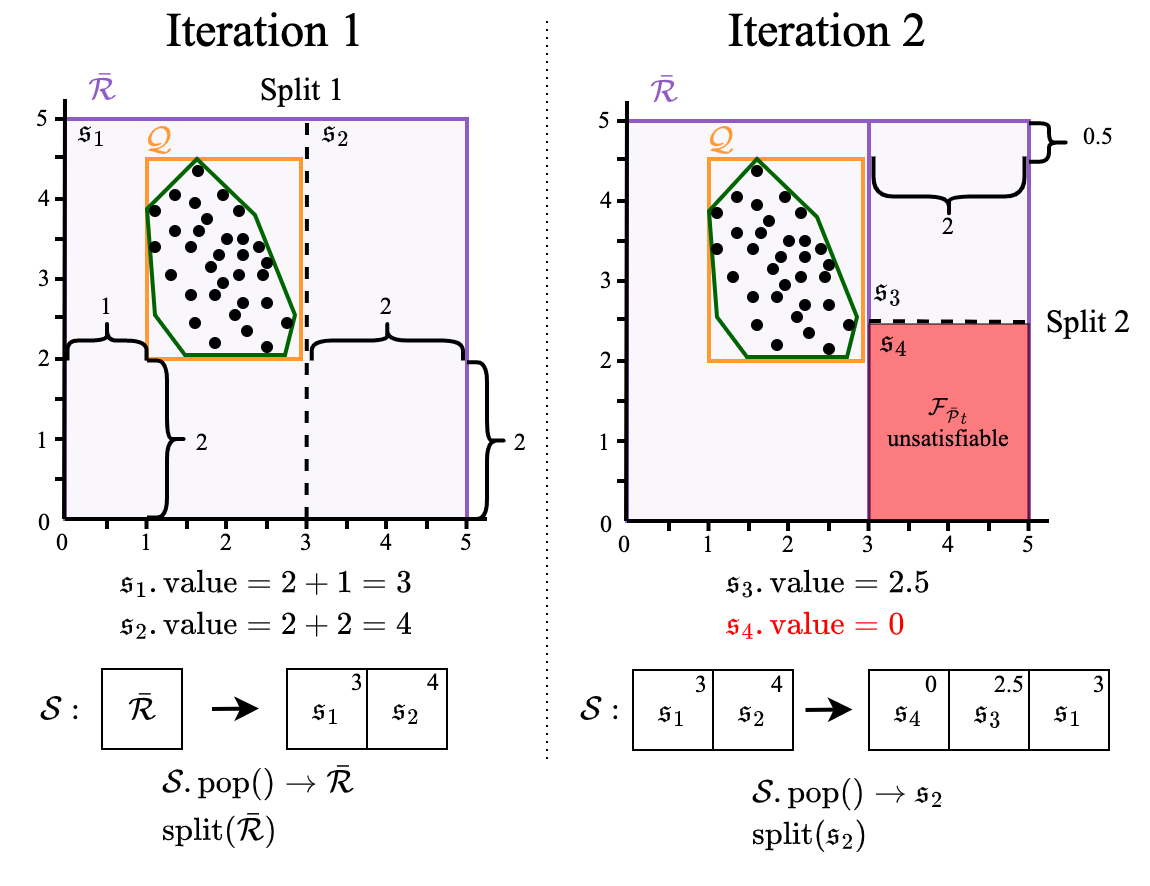
Figure 5: Two iterations of guided partitioning. In the first iteration, a split is made such that all the Monte-Carlo samples (black) that under-approximate $\mathcal{P}$ are contained in $\mathfrak{s}_{1}$. In the second iteration, $\mathfrak{s}_{2}$ is split because it is furthest from the MC sample bound $\mathcal{Q}$, and one resulting element $\mathfrak{s}_{4}$ cannot satisfy $\mathcal{F_{\bar{P}}}_{t}$. The update made to the element queue $\mathcal{S}$ is displayed for each iteration.

Finally, note that Algorithm 1 requires solving two LPs for each state. From this, it is apparent that the number of LPs solved $N_{LP}$ can be written as $N_{LP}=2n_{x}r\tau$, i.e., two LPs per state for each partition over the time horizon $\tau$. However, as $\bar{\mathcal{P}}_{t}$ is built by adding each element’s contribution $\mathcal{A}$ (15), there may be LPs that cannot possibly change $\bar{\mathcal{P}}_{t}$ because $\underaccent{\bar}{\ubar{\mathbf{x}}}_{t}\in\bar{\mathcal{P}}_{t}$ or $\bar{\bar{\mathbf{x}}}_{t}\in\bar{\mathcal{P}}_{t}$. In such cases, we can skip the irrelevant LP, thus reducing computational cost as will be shown in Section 5, where we refer to this strategy as SkipLP.

4.4 Nonlinear Dynamics: Over-Approximation of BP Sets

Algorithm 3 overviews the steps for computing backwards reachable sets when the problem dynamics are nonlinear. BReach-MILP describes a concrete approach to multi-step BP set computation where the constraints corresponding to only 1 timestep are encoded at a time. A symbolic or hybrid-symbolic [35] approach is also possible and is described in the next section. First, backreachable sets are computed. To make the optimization problem for computing the backreachable set tractable for nonlinear dynamics, we over-approximate the dynamics using OVERT [35] to obtain $\hat{p}$. With this over-approximation, the first constraint in Eq. 15 becomes a set of mixed integer constraints, and we can solve the optimization problem in Eq. 16 using a MILP solver to obtain an over-approximation of the backreachable set.

Given the backreachable set, we recompute the over-approximated dynamics model $\hat{p}$ over this smaller domain to minimize over-approximation error and decrease the number of total constraints in the optimization problem. By combining these constraints with a mixed integer encoding of the control network $\pi$ using the techniques of [24], we obtain a set of mixed integer constraints corresponding to the abstract closed-loop system $\hat{f}$. The optimization problem in Eq. 18 then becomes a MILP and can be solved using a MILP solver to obtain an over-approximated BP set.

Algorithm 3 BReach-MILP

0:  target state set $\mathcal{X}_{T}$, trained NN control policy $\pi$, time horizon $\tau$, dynamics model $p$, $\mathrm{OVERT}$ tolerance $\epsilon$

0:  BP set approximations $\bar{\mathcal{P}}_{-\tau:0}$

1:  $\bar{\mathcal{P}}_{-\tau:0}\leftarrow\emptyset$

2:  $\bar{\mathcal{P}}_{0}\leftarrow\mathcal{X}_{T}$

3:  $\hat{p}_{\mathcal{X}}\leftarrow\mathrm{OVERT}(p,\mathcal{X},\mathcal{U},\epsilon)$

4:  for $t$ in $\{-1,\ldots,-\tau\}$ do

5:     $\bar{\mathcal{R}}_{t}\!\leftarrow\!\mathrm{backreach}(\bar{\mathcal{P}}_{t\text{+}1},\mathcal{U},\mathcal{X},\hat{p}_{\mathcal{X}})$

6:     $\hat{p}\leftarrow\mathrm{OVERT}(p,\bar{\mathcal{R}}_{t},\mathcal{U},\epsilon)$

7:     $\hat{f}\leftarrow\mathrm{MIP}(\hat{p},\pi)$

8:     for $k\in n_{x}$ do

9:        $\bar{\mathbf{x}}_{t;k}\leftarrow\!\mathrm{MILPMax}(\bar{\mathcal{P}}_{t+1},\hat{f})$

10:        $\underaccent{\bar}{\mathbf{x}}_{t;k}\leftarrow\!\mathrm{MILPMin}(\bar{\mathcal{P}}_{t+1},\hat{f})$

11:     end for

12:     $\bar{\mathcal{P}}_{t}\leftarrow\{\mathbf{x}\ \lvert\ \forall k\in n_{x},\ \underaccent{\bar}{\mathbf{x}}_{t;k}\leq\mathbf{x}\leq\bar{\mathbf{x}}_{t;k}\}$

13:  end for

14:  return  $\bar{\mathcal{P}}_{-\tau:0}$

4.5 Symbolic and Hybrid-Symbolic Methods

The concrete reachability method described in Algorithm 3 compounds over-approximation error over time by creating a hyperrectangular over-approximation for each time step. A symbolic approach can alleviate this compounding. To perform symbolic reachability for systems with nonlinear dynamics, we write a symbolic equivalent to Eq. 17 as follows

$$\mathcal{F}_{\bar{\mathcal{P}}_{t}}\!\triangleq\!\left\{\!\mathbf{x}_{i}\left|\ \begin{aligned} &\mathbf{x}_{i}\in\bar{\mathcal{R}}_{i}\\ &\mathbf{x}_{i+1}\bowtie\hat{f}(\mathbf{x}_{i};\pi)\\ &\mathbf{x}_{i+1}\in\bar{\mathcal{P}}_{i+1}\\ &i\in\{t,\ldots,-1\}\end{aligned}\;\;\right.\kern-1.2pt\right\}.$$ (26)

Symbolic reachability provides tighter bounds on the BP set at the expense of a higher computational cost. For this reason, it is desirable to balance between tightness and computational efficiency. We therefore take a hybrid-symbolic approach to nonlinear backwards reachability similar to the approach described in [35]. In this approach, we reduce compounded over-approximation error by computing a symbolic set after computing a given number of concrete sets, and repeating this process iteratively.

4.6 Sources of Over-Approximation Error

To produce useful estimates for safety analysis and limit over-conservative bounds, it is important to understand and mitigate the effect of over-approximation error on the estimated BP sets. For systems with linear dynamics (Algorithm 1), the first source of over-approximation error is the linear relaxation of the NN using Theorem 3.1 to be used as constraints in the LP. Partitioning the backreachable sets, as described in Section 4.3, can reduce this error. For systems with nonlinear dynamics, on the other hand, since we solve a MILP rather than LP to compute BP sets (Algorithm 3), we can encode the network exactly using mixed-integer constraints [24]. Therefore, the network encoding does not contribute to over-approximation error in the nonlinear case. Instead, the first source of over-approximation error in Algorithm 3 is in the overapproximation of the nonlinear dynamics using piecewise-linear functions. To minimize this contribution, the piecewise-linear functions are selected to produce optimally tight bounds given a user-specified error tolerance.

The second source of over-approximation error is present in both algorithms and results from Eq. 18, which produces axis-aligned, hyper-rectangular BP sets. The use of hyper-rectanglar sets can result in large over-approximation errors if the true BP sets are not well-represented by axis-aligned hyper-rectangles. This type of error may become especially apparent when using a concrete approach as in Algorithm 3. Concretizing the BP set at each time step results in a compounding of the hyper-rectangular over-approximation error. In contrast, a symbolic approach as in Algorithm 1 encodes the dynamics constraints for all time steps in the optimization and only solves for the hyper-rectangular bounds at the time step of interest. Only concretizing the final BP set alleviates the compounding error at the expense of a more complex optimization problem. Partitioning the backwards reachable sets as in HyBReach-LP also reduces the over-approximation error due to the use of hyper-rectangular sets.

5 Numerical Results

In this section, we use numerical experiments to demonstrate HyBReach-LP and BReach-MILP and compare their properties to the algorithms proposed in [42] and to the forward reachability tool proposed in [36]. First, we show how HyBReach-LP improves upon BReach-LP and ReBReach-LP from [42] and demonstrate how the guided partitioning strategy proposed in Algorithm 2 can outperform a uniform partitioning strategy. We then demonstrate how HyBReach-LP can be used to verify safety in a collision avoidance scenario that causes the forward reachability tool Reach-LP [36] to fail. Next, we use BReach-MILP to verify safety of nonlinear version of the same collision avoidance scenario. Finally, we conduct an ablation study to show how HyBReach-LP improves the work done in [42], enabling more efficient verification of an obstacle avoidance scenario for a 6D linearized quadrotor and discuss how the proposed algorithms scale with system dimension.

All numerical results for systems with linear dynamics were collected with the LP solver cvxpy [50] on a machine running Ubuntu 20.04 with an i7-6700K CPU and 32 GB of RAM. For the experiments with nonlinear dynamics, results were obtained using the Gurobi [51] MILP solver on single Intel Core i7 4.20 GHz processor with 32 GB of RAM.

5.1 Double Integrator

Consider the discrete-time double integrator model [34]

$$\mathbf{x}_{t+1}=\underbrace{\begin{bmatrix}1&1\\ 0&1\end{bmatrix}}_{\mathbf{A}}\mathbf{x}_{t}+\underbrace{\begin{bmatrix}0.5\\ 1\end{bmatrix}}_{\mathbf{B}}\mathbf{u}_{t}$$ (27)

with $\mathbf{c}=0$, and discrete sampling time $t_{s}=1$s. The NN controller (identical to the double integrator controller used in [36]) has $[5,5]$ neurons, ReLU activations and was trained with state-action pairs generated by an MPC controller.

5.1.1 Update vs. Previous Approach

Fig. 6 compares BReach-LP (orange) and ReBReach-LP (blue) from [42] to HyBReach-LP (dashed). As shown, each algorithm collects some approximation error

$$\mathrm{error}=\frac{A_{BPE}-A_{\mathrm{true}}}{A_{\mathrm{true}}},$$ (28)

where $A_{\mathrm{true}}$ denotes the area of the tightest rectangular bound of the true BP set (dark green in Fig. 6(a)), calculated using Monte Carlo simulations, and $A_{\mathrm{BPE}}$ denotes the area of the BP estimate. As shown by Fig. 6 and Table 1, HyBReach-LP falls between BReach-LP and ReBReach-LP in terms of final step error and computation time. However, in addition to guided partitioning and the SkipLP strategy described in Section 4.3, we also improved computational efficiency from [42] by implementing disciplined parametric programming (DPP) [50] which allows cvxpy to solve large amounts of LPs more efficiently. With DPP, the time discrepancy between BReach-LP and HyBReach-LP disappears as shown by the third column of Table 1, thus leading to HyBReach-LP as the go-to strategy.

(a) BP set estimates and true BP convex hulls (dark green)

(b) Approximation error Eq. 28 calculated at each time step

Figure 6: BP set estimates for a double integrator extending from the target set (red) calculated with BReach-LP (orange) and ReBReach-LP (blue) and HyBReach-LP (dashed).

Table 1: Compare error Eq. 28 for BP algorithms.

	Runtime [s]
Algorithm	[42]	DPP+SkipLP	Final Error
BReach-LP	$1.540\pm 0.062$	$0.855\pm 0.014$	24.5
HyBReach-LP	$2.243\pm 0.043$	$0.838\pm 0.040$	4.68
ReBReach-LP	$3.410\pm 0.036$	$1.425\pm 0.043$	2.97

5.1.2 Uniform vs. Guided Partitioning

Next, we use the double integrator model to visualize how the partitioning strategy introduced in Algorithm 2 compares to the uniform strategy used in [42]. Fig. 7 first shows how each partitioning strategy performs when budgeted with different numbers of partitions. Comparing Fig. 7(a) and Fig. 7(d) shows that the guided partitioning strategy is able to converge faster than uniform partitioning. This is because guided partitioning prioritizes regions that are causing the most conservativeness in the BP set estimate. Comparing Fig. 7(c) and Fig. 7(f) demonstrates how the guided partitioning strategy is able to avoid wasting time partitioning regions of the backreachable set that are far from the true BP set.

(a) 3x3 uniform partitioning

(b) 16x16 uniform partitioning

(c) 16x16 uniform partitioning $\bar{\mathcal{P}}_{\text{-}4}$ and $\bar{\mathcal{P}}_{\text{-}5}$

(d) 9 guided partitions

(e) 256 guided partitions

(f) 256 guided partitions $\bar{\mathcal{P}}_{\text{-}4}$ and $\bar{\mathcal{P}}_{\text{-}5}$

Figure 7: Partitioning of $\bar{\mathcal{R}}_{t}$ for first and last timesteps showing that the guided partitioning strategy disregards irrelevant regions while the uniform partitioner wastes time refining regions that cannot affect $\bar{\mathcal{P}}_{t}$.

Next, Fig. 8 shows how the guided strategy is able to reduce approximation error more quickly than the uniform strategy. Notice that the guided strategy terminates the partitioning algorithm when it gets to the “best possible” solution, obtained using $100\times 100$ uniform partitions.

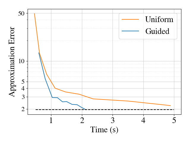
Figure 8: Guided partitioning converges to the “best possible” approximation error in 2s, whereas uniform partitioning still has not converged using $12\times 12$ partitioning with 5s of calculation time.

To explain why the best possible error using our method is not 0, we show in Fig. 9 an example of a point that satisfies the conditions from Eq. 23, but does not lie among the samples representing the true BP set. Fig. 9 shows that because the BP sets are approximated with an axis-aligned hyper-rectangle, it can be easy to step through $\bar{\mathcal{P}}$, but not through $\mathcal{P}$, leading to some conservativeness. This issue highlights the need to adapt our methods to accommodate other set representations that can more tightly approximate true BP sets, which is an interesting and practical direction for future work.

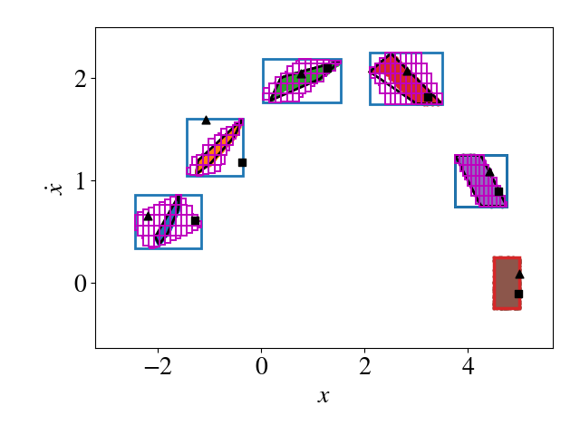
Figure 9: Example of two points that can reach $\mathcal{X}_{T}$ from $\bar{\mathcal{P}}_{-5}$ without stepping through the true BP set at each step. These points exist because Eq. 23 can only require points to go through $\bar{\mathcal{P}}_{t}$ and not $\mathcal{P}_{t}$, leading to non-zero error even with very fine partitioning.

5.2 Linearized Ground Robot

(a) Forward reachability for nominal collision avoidance scenario and vector field representation of control input. No intersection of target set (red) and reachable sets (blue) implies that safety can correctly be certified.

(b) Forward reachability for collision avoidance with bifurcating sets of trajectories. Reachable sets expand to capture both sets of possible trajectories, causing an increase in conservativeness and failure to certify safety.

(c) Backward reachability for collision avoidance with bifurcating sets of trajectories. Safety can correctly be certified because none of the BP set estimates (blue) intersect with the initial state set (black).

Figure 10: Collision avoidance situation that [36] incorrectly labels as dangerous and HyBReach-LP correctly certifies as safe.

Considering the feedback-linearization technique used in [52], we introduce the common unicycle model, represented as a pair of discrete-time integrators:

$$\mathbf{x}_{t+1}=\underbrace{\begin{bmatrix}1&0\\ 0&1\end{bmatrix}}_{\mathbf{A}}\mathbf{x}_{t}+\underbrace{\begin{bmatrix}1&0\\ 0&1\end{bmatrix}}_{\mathbf{B}}\mathbf{u}_{t},$$ (29)

with sampling time $t_{s}=1$s. Thus, state $\mathbf{x}_{t}\triangleq[p_{x},p_{y}]$ is the position of a ground robot in the $xy$-plane and the control inputs $\mathbf{u}_{t}\triangleq[v_{x},v_{y}]$ are the desired $x$ and $y$ velocity components.

To simulate the scenarios shown in Fig. 1, we trained a 2-layer NN with $[10,10]$ neurons and ReLU activations with MSE loss to imitate the vector field

$$\mathbf{u}(\mathbf{x})\text{=}\!\!\begin{bmatrix}\!\mathrm{clip}(1+\frac{2p_{x}}{p_{x}^{2}+p_{y}^{2}},-1,1)\\ \mathrm{clip}(\frac{p_{y}}{p_{x}^{2}+p_{y}^{2}}\!+\!2\mathrm{sign}(p_{y})\frac{e^{-\frac{p_{x}}{2}-2}}{(1+e^{-\frac{p_{x}}{2}-2})^{2}},-1,1)\!\end{bmatrix},$$ (30)

where $\mathrm{sign}(\cdot)$ returns the sign of the argument and $\mathrm{clip}(x,a,b)$ constrains the value of $x$ to be within $a$ and $b$. Eq. Eq. 30 was used to generate $10^{5}$ state-action pairs by sampling the state space uniformly over $\mathcal{B}_{\infty}([0,0]^{\top},[10,10]^{\top})$. The state-action pairs were then used to train the NN for 20 epochs with a batch size of 32.

As shown in Fig. 10(a), the vector field represented by Eq. 30 was designed to produce trajectories that avoid an obstacle at the origin, bounded by the target set $\mathcal{X}_{T}=\mathcal{B}_{\infty}([0,0]^{\top},[1,1]^{\top})$ (red). Fig. 10(a) also shows the forward-reachability algorithm Reach-LP [36] in a nominal obstacle-avoidance scenario where the forward reachable set estimates (blue) tightly bound the trajectories ($\mathbf{x}_{0}\rightarrow\mathbf{x}_{\tau}:\mathrm{orange}\rightarrow\mathrm{purple}$) sampled from the intial state set $\mathcal{X}_{0}=\mathcal{B}_{\infty}([-5,1]^{\top},[0.5,0.5]^{\top})$. In this case, $\mathcal{X}_{0}$ lies strictly above the $x$-axis, resulting in all possible future trajectories going above the obstacle at the origin, thus remaining bunched together and allowing forward reachability to correctly certify safety.

In Fig. 10(b), the initial state set is shifted such that it is centered on the $x$-axis, i.e., $\mathcal{X}_{0}=\mathcal{B}_{\infty}([-5,0]^{\top},[0.5,0.5]^{\top})$. This causes the NN control policy to command the system to go above the obstacle for some states in $\mathcal{X}_{0}$ while others go below. The resulting forward reachability analysis shows a drastically different picture than Fig. 10(a), with the forward reachable sets quickly gaining conservativeness as they encompass both sets of possible trajectories. While other forward reachability analysis tools [35] may reduce conservativeness in the upper- and lower-bounds of the reachable set estimates, we are not aware of any methods to consider the space between the sets of trajectories, which is the region that intersects with the obstacle and causes safety certification to fail. Also note that while an alternative strategy could be to partition $\mathcal{X}_{0}$ such that each element goes in one of the two directions, this would require a perfect split along the learned decision boundary, which would be challenging in practice.

Finally, Fig. 10(c) shows the same situation as Fig. 10(b), but now we use the backward reachability approach described in Section 4.2 as the strategy for safety certification. Instead of propagating forward from $\mathcal{X}_{0}$, the states that lead to $\mathcal{X}_{T}$ are calculated using HyBReach-LP with 12 guided partitions to give BP over-approximations (blue). Since the control policy was designed to force the system away from the obstacle bounded by $\mathcal{X}_{T}$, the BP over-approximations remain close to $\mathcal{X}_{T}$ (red) and do not intersect with $\mathcal{X}_{0}$ (black), thus successfully certifying safety for the situation shown. Note that while the forward reachable sets in Fig. 10(b) were calculated in 0.5s compared to 2.0s for the BP over-approximations in Fig. 10(c), the result given by HyBReach-LP is more useful.

Fig. 11 shows that, in addition to certifying safe situations, HyBReach-LP can also be used to detect failures in a trained control policy. The policy shown in Fig. 11 was trained using a modified version of Eq. 30 that causes the policy to lead the system to the origin for some states. Given this “bug” in the policy, the BP over-approximations now expand out to include $\mathcal{X}_{0}$, implying that if the system is in $\mathcal{X}_{0}$, it is possible to collide with the obstacle.

Figure 11: HyBReach-LP is does not certify safety for a faulty NN control policy.

5.3 Nonlinear Ground Robot

We represent a nonlinear version of the ground robot shown in Section 5.2 by changing the dynamics as follows

$$p_{x,t+1}=p_{x,t}+v_{t}\cos(\theta_{t})$$ (31)

$$p_{y,t+1}=p_{y,t}+v_{t}\sin(\theta_{t})$$

with sampling time $t_{s}=1$s. The state is still represented by $\mathbf{x}=[p_{x},p_{y}]^{\top}$, but the control inputs are now $\mathbf{u}=[v,\theta]^{\top}$ making the dynamics nonlinear in the control inputs due to the multiplicative and trigonometric operations in Eq. 31. The velocity and heading control inputs are derived from the vector field described in Eq. 30 and shown in Fig. 10(a). A NN with three hidden layers containing $10$ units each and ReLU activations was trained using $1.01\times 10^{6}$ data points generated from the state space region $\mathcal{B}_{\infty}([0,0]^{\top},[6,6]^{\top})$ to replicate the vector field in Eq. 30. Data points were more densely sampled near critical regions of the state space (e.g., avoid set). The network was trained for $250$ epochs with a batch size of $512$ and a mean squared error (MSE) loss function.

We can apply forward reachability to assess safety in this scenario using the techniques described by [35]. However, a forward reachability analysis will behave similarly to the results shown for the linear case in Figs. 10(a) and 10(b), and this scenario, therefore, requires a backward reachability analysis to make a useful safety assessment. Figure 12 shows the results of applying BReach-MILP to generate BP sets with $\tau=9$. Since the overapproximated BP sets do not intersect with the initial set, we can verify safety over this time horizon.

Figure 12: Backward reachability analysis for collision avoidance for a nonlinear 2D robot. The controller is certified safe as the backprojection sets (blue) do not intersect with the initial set (black).

We note that the BP sets for the nonlinear ground robot shown in Fig. 12 do not behave similarly to the BP sets for the linear ground robot shown in Fig. 10(c). In particular, while the BP sets for the linear ground robot all remain relatively close to the avoid set, the BP sets for the nonlinear ground robot appear to march to the right in a direction pointed away from the avoid set. This discrepancy provides insight into a potential vulnerability of the system. In particular, the BP sets shown in Fig. 12 indicate that there must be some control outputs near the $x$-axis that cause the robot to move directly to the left and into the avoid set.

Figure 13 confirms this hypothesis by showing samples from the first BP set that reach the avoid set when simulated one step forward in time. Upon further analysis, we were able to attribute this behavior to angle wraparound. Since we chose to represent $\theta$ using values between $0$ and $2\pi$ radians (where $0$ and $2\pi$ both represent a heading pointing to the right in the $+x$ direction), the vector field in Eq. 30 causes inputs just above the $x$-axis to have an angle near $0$ and inputs just below the $x$-axis to have an angle near $2\pi$. Since ReLU networks represent piecewise continuous functions, there must exist a point near the $x$-axis where the control network commands a heading of $\pi$. A heading of $\pi$ causes the robot to point in the $-x$ direction and therefore towards the avoid set, resulting in the rightward marching of the BP sets in Fig. 12. This insight is critical in informing future designs of the system. For instance, if we had instead parameterized $\theta$ to use values between $-\pi$ and $\pi$, this vulnerability would occur on the negative portion of the $x$-axis and cause the BP sets to march leftward and intersect with the initial set, ultimately resulting in an unsafe system.

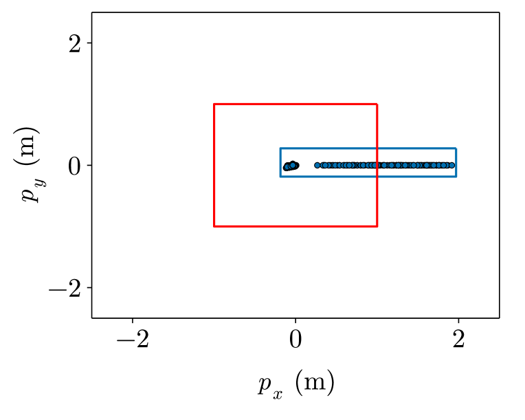
Figure 13: Samples from the one-step BP set (blue) for the nonlinear ground robot that reach the avoid set.

While concrete multi-step backward reachability (as shown in Fig. 12) provided sufficient accuracy for verifying safety, we also tested a hybrid-symbolic approach similar to that described by [35] for an arbitrary target set. Figure 14 visualizes the results of performing a symbolic step after every third concrete step. Each set of samples approximates the true BP set at the given time step. In general, the bounds lose tightness over time due to both the accumulation of over-approximation error from the concrete steps and the fact that the true BP sets become less rectangular in shape over time. Nevertheless, the symbolic sets (solid) provide tighter overapproximations than the concrete sets (dashed).

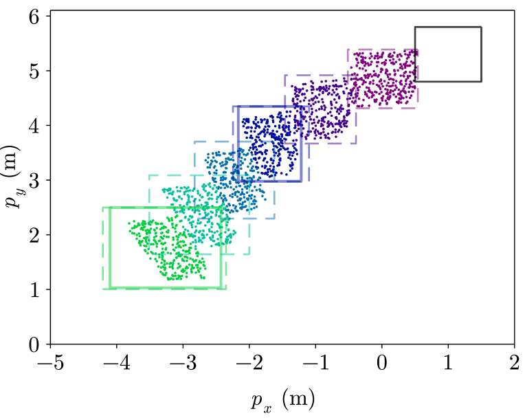
Figure 14: Visualization of concrete (dashed) and symbolic (solid) over-appoximated BP sets corresponding to the target set shown in back. Samples to approximate the true target set were obtained by sampling $50,000$ points uniformly inside the domain and checking for simulations that reach the target set.

5.4 Ablation Study: Linearized Quadrotor

To investigate how our algorithm scales with the state space, we next consider a 6-dimensional linearized quadrotor model. By representing the quadrotor as three double integrators corresponding to the vehicle’s $x-y-z$ coordinates, we obtain the model

$$\mathbf{x}_{t+1}=\underbrace{\begin{bmatrix}1&0&0&1&0&0\\ 0&1&0&0&1&0\\ 0&0&1&0&0&1\\ 0&0&0&1&0&0\\ 0&0&0&0&1&0\\ 0&0&0&0&0&1\\ \end{bmatrix}}_{\mathbf{A}}\mathbf{x}_{t}+\underbrace{\begin{bmatrix}0.5&0&0\\ 0&0.5&0\\ 0&0&0.5\\ 1&0&0\\ 0&1&0\\ 0&0&1\\ \end{bmatrix}}_{\mathbf{B}}\mathbf{u}_{t}.$$ (32)

In a similar way to Section 5.2, we trained a control policy with $[20,20]$ ReLU-activated neurons by specifying a vector field that avoids an obstacle placed at $\mathcal{X}_{T}=\mathcal{B}_{\infty}([0,0,2.5,0,0,0]^{\top},[1,1,1,1,1,1]^{\top})$. The vector field is represented by the equations

$$\mathbf{u}=\begin{cases}4\mathrm{sign}(\mathbf{p})\quad&\|\mathbf{p}\|_{\infty}<2.25\\ \begin{bmatrix}0\\ \mathrm{clip}(\frac{4}{p_{y}}-\frac{p_{y}}{4}-3v_{y},-2,2)\\ 0\\ \end{bmatrix}\quad&\|\mathbf{p}\|_{\infty}\geq 2.25.\end{cases}$$ (33)

Fig. 15 shows simulated trajectories using the controller trained with Eq. 33 propagated from an initial condition at $\mathcal{X}_{0}=\mathcal{B}_{\infty}([-5,0,2.5,0.97,0,0]^{\top},$ $[0.25,0.25,0.25,0.02,0.01,0.01]^{\top})$ with $dt=1$ over a time horizon $\tau=6$. Like Fig. 10(c), the BP set estimates (blue), obtained with Algorithm 1 using $r=750$ do not intersect with the initial state set, thus proving safety in this scenario. This is confirmed by observing that the simulated trajectories do not intersect with the obstacle (red). Note that while BP over-approximations are calculated through $\tau=6$, the fact that the first BP over-approximation is fully contained within the target set implies that all subsequent BP over-approximations should also fall within the target set, allowing us to stop after the calculation of the first BP over-approximation. The idea that $\bar{\mathcal{P}}_{t}\!\subseteq\!\mathcal{P}_{t+1}$ leads to a form of invariance is stated formally and proven in Section .2.

Figure 15: Verification of 6-dimensional quadrotor system during obstacle avoidance maneuver.

To help quantify the improvements in computation time made to our approach when compared with [42], we replicated the scenario showed in Fig. 15 with several different configurations of HyBReach-LP. Table 2 shows the results of our comparison. Note that rows using a uniform partitioning strategy split each state into 5 partitions (resulting in $5^{6}$ total elements), which is the smallest amount capable of correctly verifying safety. The first row represents [42] with the exception that it uses HyBReach-LP rather than BReach-LP or ReBReach-LP. The second row makes use of disciplined parametric programming (DPP) [50], which allows cvxpy to solve many LPs more efficiently. Finally, the third row includes the SkipLP strategy described in Section 4.3 and the last row uses all components together with the guided partitioning strategy described in Algorithm 2.

Table 2: Ablation study showing the computational cost of calculating Fig. 15 with different combinations of DPP, SkipLP, and guided partitioning.

Configuration	Runtime [s]
Uniform [42]	$3796$
Uniform + DPP	$2064$
Uniform + DPP + SkipLP	$1365$
Guided + DPP + SkipLP	$28$

6 Conclusion

In this paper, we considered the problem of backward reachability for NFLs. We presented an algorithm that combines the best elements of the two algorithms proposed by [42] to calculate over-approximations of BP sets over a given time horizon for systems with linear dynamics. We also introduced a new algorithm to compute over-approximations of the BP sets for nonlinear dynamical systems. We highlighted the advantages of backward reachability on both linear and nonlinear versions of a 2D collision avoidance system. We also demonstrated reduced computation time by introducing a guided partitioning strategy that more intelligently divides up the input space to the NN relaxation used to find the BP sets. These improvements were used to verify a 6D linearized quadrotor system over 100 times faster than the previous method.

.1 Proof of 4.1

See 4.1

Proof .1.

Consider the calculation of the first BP set over-approximation $\bar{\mathcal{P}}_{-1}$. Using Eq. 22, we first calculate $\bar{\mathcal{R}}_{-1}$, which is guaranteed to contain all the states for which the system can arrive in $\mathcal{X}_{T}$ given $\mathbf{u}\in\mathcal{U}$ and $\mathbf{x}\in\mathcal{X}$. Notice that $\bar{\mathcal{P}}_{-1}\subseteq\bar{\mathcal{R}}_{-1}$, which allows us to apply Theorem 3.1 over $\bar{\mathcal{R}}_{-1}$ to obtain bounds $\pi^{L}_{-1}(\mathbf{x})$ and $\pi^{U}_{-1}(\mathbf{x})$ that are valid over $\mathcal{P}_{-1}$. We then use Eq. 23 to include the constraint that $\pi^{L}_{-1}(\mathbf{x})\leq\mathbf{u}_{-1}\leq\pi^{U}_{-1}(\mathbf{x})$, which is guaranteed by Theorem 3.1 to satisfy $\pi^{L}_{-1}(\mathbf{x}_{-1})\leq\pi(\mathbf{x})\leq\pi^{U}_{-1}(\mathbf{x}_{-1})$. From this we can conclude that

$$\bar{\mathcal{P}}_{-1}(\mathcal{X}_{T})= \ \{\mathbf{x}\ |\ \underaccent{\bar}{\x}_{-1}\leq\mathbf{x}\leq\bar{\mathbf{x}}_{-1}\}$$ (34)

$$\begin{split}\supseteq&\ \{\mathbf{x}\ |\ f(\mathbf{x},\mathbf{u})\in\mathcal{X}_{T},\ \\ &\quad\quad\quad\quad\pi^{L}_{-1}(\mathbf{x})\leq\mathbf{u}\leq\pi^{U}_{-1}(\mathbf{x})\},\end{split}$$ (35)

$$\supseteq \ \{\mathbf{x}\ \lvert\ f(\mathbf{x},\pi(\mathbf{x}))\in\mathcal{X}_{T}\}=\mathcal{P}_{-1}(\mathcal{X}_{T}),$$ (36)

thus proving 4.1 for the first time step. This gives us the result that all states that reach $\mathcal{X}_{T}$ must get there by applying a control value satisfying $\pi^{L}_{-1}(\mathbf{x})\leq\mathbf{u}_{-1}\leq\pi^{U}_{-1}(\mathbf{x})$ from somewhere in $\bar{\mathcal{P}}_{-1}$.

Now if we consider Eq. 24 for $t=-2$, i.e.,

$$\bar{\mathcal{P}}_{-2}(\mathcal{X}_{T})= \ \{\mathbf{x}_{-2}\ |\ \underaccent{\bar}{\x}_{-2}\leq\mathbf{x}_{-2}\leq\bar{\mathbf{x}}_{-2}\}$$ (37)

$$\begin{split}\supseteq&\ \{\mathbf{x}_{-2}\ |\ \mathbf{x}_{-1}=f(\mathbf{x}_{-2},\mathbf{u}_{-2})\in\bar{\mathcal{P}}_{-1},\ \\ &\quad\quad\quad\ f(\mathbf{x}_{-1},\mathbf{u_{-1}})\in\mathcal{X}_{T},\ \\ &\quad\quad\quad\ \pi^{L}_{-2}(\mathbf{x})\leq\mathbf{u}_{-2}\leq\pi^{U}_{-2}(\mathbf{x}),\\ &\quad\quad\quad\ \pi^{L}_{-1}(\mathbf{x})\leq\mathbf{u}_{-1}\leq\pi^{U}_{-1}(\mathbf{x})\},\end{split}$$ (38)

$$\begin{split}\supseteq&\ \{\mathbf{x}_{-2}\ \lvert\ \mathbf{x}_{-1}=f(\mathbf{x}_{-2},\pi(\mathbf{x}_{-2}))\in\mathcal{P}_{-1},\\ &f(\mathbf{x}_{-1},\pi(\mathbf{x}_{-1}))\in\mathcal{X}_{T},\}=\mathcal{P}_{-2}(\mathcal{X}_{T}),\end{split}$$ (39)

it becomes clear that because $\mathcal{P}_{-1}(\mathcal{X}_{T})\subseteq\bar{\mathcal{P}}_{-1}(\mathcal{X}_{T})$, and with bounds on the control limits from Theorem 3.1, we can conclude that $\mathcal{P}_{-2}(\mathcal{X}_{T})\subseteq\bar{\mathcal{P}}_{-2}(\mathcal{X}_{T})$. From here, the same argument can be applied an arbitrary number of time steps backward, allowing us to conclude

$$\mathcal{P}_{t}(\mathcal{X}_{T})\subseteq\bar{\mathcal{P}}_{t}(\mathcal{X}_{T})\quad\forall t\in\mathcal{T}.$$ (40)

.2 Backward Invariance

Lemma .2.

If there exists a BP over-approximation $\bar{\mathcal{P}}_{t_{2}}$ and a concrete set $\mathcal{P}_{t_{1}}$ at times $t_{1},t_{2}$ with $t_{2}<t_{1}\leq 0$, such that $\bar{\mathcal{P}}_{t_{2}}\subseteq\mathcal{P}_{t_{1}}$, then

$$\mathcal{I}=\mathcal{P}_{t_{1}}\cup\bigcup_{t=t_{2}}^{t_{1}-1}\bar{\mathcal{P}}_{t}$$ (41)

contains all BP sets for $t\leq t_{1}$, i.e., $\bar{\mathcal{P}}_{t}\subseteq\mathcal{I}\ \forall t\leq t_{1}$.

Proof .3.

This is a proof by induction where we wish to show that for any $t\leq t_{2}$, $\mathcal{P}_{t}\subseteq\mathcal{I}$. To prove the base case, we simply have to show that $\mathcal{P}_{t_{2}}\subseteq\mathcal{I}$. Given that $\mathcal{P}_{t_{2}}\subseteq\bar{\mathcal{P}}_{t_{2}}$ and that $\mathcal{I}=\mathcal{P}_{t_{1}}\cup\dots\cup\bar{\mathcal{P}}_{t_{2}}$, it must be that $\mathcal{P}_{t_{2}}\subseteq\mathcal{I}$.

To show the inductive step, we need to show that for any $t<t_{2}$, $\mathcal{P}_{t}\subseteq\mathcal{I}$. First note that given $\bar{\mathcal{P}}_{t_{2}}\subseteq\mathcal{P}_{t_{1}}$ and that $\mathcal{P}_{t_{2}}\subseteq\bar{\mathcal{P}}_{t_{2}}$, we know that $\mathcal{P}_{t_{2}}\subseteq\mathcal{P}_{t_{1}}$. It then follows that $\mathcal{P}_{t_{2}-1}\subseteq\mathcal{P}_{t_{1}-1}$ because if $\mathcal{P}_{t_{2}}\subseteq\mathcal{P}_{t_{1}}$, any state that leads to $\mathcal{P}_{t_{2}}$ must also lead to $\mathcal{P}_{t_{1}}$. This argument can be applied iteratively to obtain

$$\begin{split}\mathcal{P}_{t_{2}-1}&\subseteq\mathcal{P}_{t_{1}-1}\\ \mathcal{P}_{t_{2}-2}&\subseteq\mathcal{P}_{t_{1}-2}\\ &\ \vdots\\ \mathcal{P}_{t_{2}-\Delta t}&\subseteq\mathcal{P}_{t_{1}-\Delta t}.\end{split}$$

By selecting $\Delta t\triangleq t_{1}-t_{2}$, we can make the substitution $\mathcal{P}_{t_{1}-\Delta t}=\mathcal{P}_{t_{2}}$ to get

$$\mathcal{P}_{t_{2}-\Delta t}\subseteq\mathcal{P}_{t_{2}}\subseteq\mathcal{P}_{t_{1}}.$$

It follows that $\mathcal{P}_{t}\subseteq\mathcal{P}_{t+\Delta t}\ \forall t\leq t_{2}$. If we assume that $\bar{\mathcal{P}}_{i}\subseteq\mathcal{I}\ \forall i\in\{t+1,\dots t_{2}\}$, then we get $\mathcal{P}_{t}\subseteq\mathcal{P}_{t+\Delta t}\subseteq\bar{\mathcal{P}}_{t+\Delta t}\subseteq\mathcal{I}$, thus proving the inductive step.

Corollary .4.

If there exists a BP overapproximation at time $t=-1$ such that $\bar{\mathcal{P}}_{-1}\subseteq\mathcal{X}_{T}$, then $\mathcal{X}_{T}$ contains all BP sets with $t\leq t_{1}$, i.e., $\mathcal{X}_{T}\subseteq\mathcal{I}\ \forall t\leq t_{1}$, thus rendering $\mathcal{X}_{T}$ an invariant set.

References

- [1] Jie Tan, Tingnan Zhang, Erwin Coumans, Atil Iscen, Yunfei Bai, Danijar Hafner, Steven Bohez and Vincent Vanhoucke “Sim-to-Real: Learning Agile Locomotion For Quadruped Robots.” In Robotics: Science and Systems, 2018
- [2] Joonho Lee, Jemin Hwangbo, Lorenz Wellhausen, Vladlen Koltun and Marco Hutter “Learning quadrupedal locomotion over challenging terrain” In Science Robotics 5.47 American Association for the Advancement of Science, 2020, pp. eabc5986
- [3] Jemin Hwangbo, Inkyu Sa, Roland Siegwart and Marco Hutter “Control of a quadrotor with reinforcement learning” In IEEE Robotics and Automation Letters 2.4 IEEE, 2017, pp. 2096–2103
- [4] Shixiang Gu, Ethan Holly, Timothy Lillicrap and Sergey Levine “Deep reinforcement learning for robotic manipulation with asynchronous off-policy updates” In IEEE International Conference on Robotics and Automation (ICRA), 2017, pp. 3389–3396
- [5] Dmitry Kalashnikov, Alex Irpan, Peter Pastor, Julian Ibarz, Alexander Herzog, Eric Jang, Deirdre Quillen, Ethan Holly, Mrinal Kalakrishnan and Vincent Vanhoucke “Scalable deep reinforcement learning for vision-based robotic manipulation” In Conference on Robot Learning (CoRL), 2018, pp. 651–673
- [6] Gene F Franklin, J David Powell and Abbas Emami-Naeini “Feedback Control of Dynamic Systems”, 2014
- [7] Lars Grüne and Jürgen Pannek “Nonlinear Model Predictive Control” In Nonlinear Model Predictive Control: Theory and Algorithms Springer, 2017
- [8] Alexey Kurakin, Ian J. Goodfellow and Samy Bengio “Adversarial examples in the physical world” In International Conference on Learning Representations (ICLR) Workshop Track Proceedings, 2017 URL: https://openreview.net/forum?id=HJGU3Rodl
- [9] Xiaoyong Yuan, Pan He, Qile Zhu and Xiaolin Li “Adversarial examples: Attacks and defenses for deep learning” In IEEE Transactions on Neural Networks and Learning Systems 30.9 IEEE, 2019, pp. 2805–2824
- [10] Chenyi Chen, Ari Seff, Alain Kornhauser and Jianxiong Xiao “Deepdriving: Learning affordance for direct perception in autonomous driving” In International Conference on Computer Vision (ICCV), 2015, pp. 2722–2730
- [11] Alex Kendall, Jeffrey Hawke, David Janz, Przemyslaw Mazur, Daniele Reda, John-Mark Allen, Vinh-Dieu Lam, Alex Bewley and Amar Shah “Learning to drive in a day” In IEEE International Conference on Robotics and Automation (ICRA), 2019, pp. 8248–8254
- [12] Michael Kelly, Chelsea Sidrane, Katherine Driggs-Campbell and Mykel J Kochenderfer “HG-DAgger: Interactive imitation learning with human experts” In IEEE International Conference on Robotics and Automation (ICRA), 2019, pp. 8077–8083
- [13] Kyle D Julian, Mykel J Kochenderfer and Michael P Owen “Deep neural network compression for aircraft collision avoidance systems” In Journal of Guidance, Control, and Dynamics 42.3 American Institute of AeronauticsAstronautics, 2019, pp. 598–608
- [14] Ya-Chien Chang, Nima Roohi and Sicun Gao “Neural Lyapunov control” In Advances in Neural Information Processing Systems (NeurIPS) 32, 2019
- [15] Dawei Sun, Susmit Jha and Chuchu Fan “Learning certified control using contraction metric” In Conference on Robot Learning, 2021, pp. 1519–1539 PMLR
- [16] Minghao Han, Lixian Zhang, Jun Wang and Wei Pan “Actor-critic reinforcement learning for control with stability guarantee” In IEEE Robotics and Automation Letters 5.4 IEEE, 2020, pp. 6217–6224
- [17] Zengyi Qin, Kaiqing Zhang, Yuxiao Chen, Jingkai Chen and Chuchu Fan “Learning Safe Multi-agent Control with Decentralized Neural Barrier Certificates” In International Conference on Learning Representations, 2020
- [18] H. Dai, B. Landry, L. Yang, M. Pavone and R. Tedrake “Lyapunov-Stable Neural-Network Control” In Robotics: Science and Systems, 2021 URL: https://arxiv.org/pdf/2109.14152.pdf
- [19] Charles Dawson, Sicun Gao and Chuchu Fan “Safe Control with Learned Certificates: A Survey of Neural Lyapunov, Barrier, and Contraction methods” In arXiv preprint arXiv:2202.11762, 2022
- [20] Huan Zhang, Tsui-Wei Weng, Pin-Yu Chen, Cho-Jui Hsieh and Luca Daniel “Efficient neural network robustness certification with general activation functions” In Advances in Neural Information Processing Systems (NeurIPS), 2018
- [21] Lily Weng, Huan Zhang, Hongge Chen, Zhao Song, Cho-Jui Hsieh, Luca Daniel, Duane Boning and Inderjit Dhillon “Towards fast computation of certified robustness for relu networks” In International Conference on Machine Learning (ICML), 2018, pp. 5276–5285
- [22] Kaidi Xu, Zhouxing Shi, Huan Zhang, Yihan Wang, Kai-Wei Chang, Minlie Huang, Bhavya Kailkhura, Xue Lin and Cho-Jui Hsieh “Automatic perturbation analysis for scalable certified robustness and beyond” In Advances in Neural Information Processing Systems (NeurIPS) 33, 2020, pp. 1129–1141
- [23] Aditi Raghunathan, Jacob Steinhardt and Percy S Liang “Semidefinite relaxations for certifying robustness to adversarial examples” In Advances in Neural Information Processing Systems (NeurIPS) 31, 2018
- [24] Vincent Tjeng, Kai Y Xiao and Russ Tedrake “Evaluating Robustness of Neural Networks with Mixed Integer Programming” In International Conference on Learning Representations, 2018
- [25] Guy Katz, Derek A Huang, Duligur Ibeling, Kyle Julian, Christopher Lazarus, Rachel Lim, Parth Shah, Shantanu Thakoor, Haoze Wu and Aleksandar Zeljić “The marabou framework for verification and analysis of deep neural networks” In International Conference on Computer Aided Verification, 2019, pp. 443–452
- [26] Guy Katz, Clark Barrett, David L Dill, Kyle Julian and Mykel J Kochenderfer “Reluplex: An efficient SMT solver for verifying deep neural networks” In International Conference on Computer-Aided Verification (CAV), 2017, pp. 97–117
- [27] Kai Jia and Martin Rinard “Verifying Low-Dimensional Input Neural Networks via Input Quantization” In International Static Analysis Symposium, 2021, pp. 206–214
- [28] Joseph A Vincent and Mac Schwager “Reachable polyhedral marching (RPM): A safety verification algorithm for robotic systems with deep neural network components” In IEEE International Conference on Robotics and Automation (ICRA), 2021, pp. 9029–9035
- [29] Souradeep Dutta, Xin Chen and Sriram Sankaranarayanan “Reachability analysis for neural feedback systems using regressive polynomial rule inference” In International Conference on Hybrid Systems: Computation and Control, 2019, pp. 157–168
- [30] Chao Huang, Jiameng Fan, Wenchao Li, Xin Chen and Qi Zhu “Reachnn: Reachability analysis of neural-network controlled systems” In ACM Transactions on Embedded Computing Systems (TECS) 18.5s ACM New York, NY, USA, 2019, pp. 1–22
- [31] Radoslav Ivanov, James Weimer, Rajeev Alur, George J Pappas and Insup Lee “Verisig: verifying safety properties of hybrid systems with neural network controllers” In International Conference on Hybrid Systems: Computation and Control, 2019, pp. 169–178
- [32] Jiameng Fan, Chao Huang, Xin Chen, Wenchao Li and Qi Zhu “Reachnn*: A tool for reachability analysis of neural-network controlled systems” In International Symposium on Automated Technology for Verification and Analysis, 2020, pp. 537–542
- [33] Weiming Xiang, Hoang-Dung Tran, Xiaodong Yang and Taylor T Johnson “Reachable set estimation for neural network control systems: A simulation-guided approach” In IEEE Transactions on Neural Networks and Learning Systems 32.5 IEEE, 2020, pp. 1821–1830
- [34] Haimin Hu, Mahyar Fazlyab, Manfred Morari and George J Pappas “Reach-SDP: Reachability analysis of closed-loop systems with neural network controllers via semidefinite programming” In IEEE Conference on Decision and Control (CDC), 2020, pp. 5929–5934
- [35] Chelsea Sidrane, Amir Maleki, Ahmed Irfan and Mykel J Kochenderfer “OVERT: An algorithm for safety verification of neural network control policies for nonlinear systems” In Journal of Machine Learning Research 23.117, 2022, pp. 1–45
- [36] Michael Everett, Golnaz Habibi, Chuangchuang Sun and Jonathan P How “Reachability Analysis of Neural Feedback Loops” In IEEE Access 9 IEEE, 2021, pp. 163938–163953
- [37] Shaoru Chen, Victor M Preciado and Mahyar Fazlyab “One-Shot Reachability Analysis of Neural Network Dynamical Systems” In arXiv preprint arXiv:2209.11827, 2022
- [38] Stanley Bak and Hoang-Dung Tran “Neural Network Compression of ACAS Xu Early Prototype Is Unsafe: Closed-Loop Verification Through Quantized State Backreachability” In NASA Formal Methods, 2022, pp. 280–298
- [39] Somil Bansal, Mo Chen, Sylvia Herbert and Claire J Tomlin “Hamilton-Jacobi reachability: A brief overview and recent advances” In IEEE Conference on Decision and Control (CDC), 2017, pp. 2242–2253
- [40] Lawrence C Evans “Partial differential equations” American Mathematical Soc., 2010
- [41] Ian M Mitchell “Comparing forward and backward reachability as tools for safety analysis” In International Workshop on Hybrid Systems: Computation and Control, 2007, pp. 428–443
- [42] Nicholas Rober, Michael Everett and Jonathan P. How “Backward Reachability Analysis of Neural Feedback Loops” (to appear) In IEEE Conference on Decision and Control (CDC), 2022 URL: https://arxiv.org/abs/2204.08319
- [43] Matthias Althoff “An introduction to CORA 2015” In Workshop on Applied Verification for Continuous and Hybrid systems, 2015, pp. 120–151
- [44] Xin Chen, Erika Ábrahám and Sriram Sankaranarayanan “Flow*: An analyzer for non-linear hybrid systems” In International Conference on Computer-Aided Verification (CAV), 2013, pp. 258–263
- [45] Goran Frehse, Colas Le Guernic, Alexandre Donzé, Scott Cotton, Rajarshi Ray, Olivier Lebeltel, Rodolfo Ripado, Antoine Girard, Thao Dang and Oded Maler “SpaceEx: Scalable verification of hybrid systems” In International Conference on Computer-Aided Verification (CAV), 2011, pp. 379–395
- [46] Stanley Bak and Parasara Sridhar Duggirala “HYLAA: A tool for computing simulation-equivalent reachability for linear systems” In International Conference on Hybrid Systems: Computation and Control, 2017, pp. 173–178
- [47] Parasara Sridhar Duggirala, Sayan Mitra, Mahesh Viswanathan and Matthew Potok “C2E2: A verification tool for stateflow models” In International Conference on Tools and Algorithms for the Construction and Analysis of Systems, 2015, pp. 68–82
- [48] Lynton Ardizzone, Jakob Kruse, Carsten Rother and Ullrich Köthe “Analyzing Inverse Problems with Invertible Neural Networks” In International Conference on Learning Representations, 2018
- [49] Jens Behrmann, Will Grathwohl, Ricky TQ Chen, David Duvenaud and Jörn-Henrik Jacobsen “Invertible residual networks” In International Conference on Machine Learning (ICML), 2019, pp. 573–582
- [50] Steven Diamond and Stephen Boyd “CVXPY: A Python-embedded modeling language for convex optimization” In Journal of Machine Learning Research 17.1 JMLR. org, 2016, pp. 2909–2913
- [51] Gurobi Optimization, LLC “Gurobi Optimizer Reference Manual”, 2022 URL: https://www.gurobi.com
- [52] Jose Bernardo Martinez, Hector M Becerra and David Gomez-Gutierrez “Formation Tracking Control and Obstacle Avoidance of Unicycle-Type Robots Guaranteeing Continuous Velocities” In Sensors 21.13 Multidisciplinary Digital Publishing Institute, 2021, pp. 4374