A Stiff MOL Boundary Control Problem for the 1D Heat Equation with Exact Discrete Solution

Abstract

Method-of-lines discretizations are demanding test problems for stiff integration methods. However, for PDE problems with known analytic solution the presence of space discretization errors or the need to use codes to compute reference solutions may limit the validity of numerical test results. To overcome these drawbacks we present in this short note a simple test problem with boundary control, a situation where one-step methods may suffer from order reduction. We derive exact formulas for the solution of an optimal boundary control problem governed by a one-dimensional discrete heat equation and an objective function that measures the distance of the final state from the target and the control costs. This analytical setting is used to compare the numerically observed convergence orders for selected implicit Runge-Kutta and Peer two-step methods of classical order four which are suitable for optimal control problems.

Key words. Optimal control, implicit Peer two-step methods, first-discretize-then-optimize, discrete adjoints

1 Introduction

One main area of application for stiff integration methods is semi-discretizations in space of time-dependent partial differential equations in the method-of-lines approach. In order to test new methods in this area one may rely on PDE test problems with known analytic solution or reference solutions computed by other numerical methods. However, both approaches have its drawbacks. For PDE problems the accuracy is limited by the level of space discretization errors and in computing reference solutions one has to trust the reliability of the used code. This background was our motivation to develop the current test problems with exact discrete solutions for a finite difference semi-discretization in space with arbitrarily fine grids.

It is known that, in contrast to multi-step type methods, one-step methods may suffer from order reduction if applied to MOL systems especially with time-dependent boundary conditions, see [6, 7]. Motivated by our recent work [4, 5] on Peer two-step methods in optimal control the present example is formulated as a problem with boundary control.

The paper is organized as follows. In Section 2, we apply a finite difference discretization with a shifted equi-spaced grid for the 1D heat equation with general Robin boundary conditions and derive exact formulas for the solutions of the discrete heat equation and an optimal boundary control problem. These analytical solutions are used in a sparse setting to study the numerically observed convergence orders in Section 3 for several one-step and two-step integration methods which are suitable for optimal control.

2 A discrete heat equation with boundary control

2.1 Finite difference discretization of the 1D heat equation

We consider the initial-boundary-value problem for a function $Y(x,t)$ governed by the heat equation

$$\partial_{t}Y(x,t)= \,\partial_{xx}Y(x,t),\ (x,t)\in[0,1]\times[0,T],$$ (1)

$$\partial_{x}Y(0,t)= \,0,\;\beta_{0}Y(1,t)+\beta_{1}\partial_{x}Y(1,t)=u(t),$$ (2)

$$Y(x,0)= \,\Psi(x),$$ (3)

where $\Psi(x)$ and $u(t)$ are given functions. The homogeneous Neumann condition at $x=0$ may be considered as a short-cut for space-symmetric solutions $Y(-x,t)\equiv Y(x,t)$. The coefficients of the general Robin boundary condition are nonnegative, $\beta_{0},\beta_{1}\geq 0$ and nontrivial $(\beta_{0},\beta_{1})\not=(0,0)$.

The equation (1) is approximated by finite differences with a shifted equi-spaced grid with stepsize $\xi=1/m$, $m\in{\mathbb{N}}$:

$$x_{j}=\left(j-\frac{1}{2}\right)\xi,\ j=1,\ldots,m.$$ (4)

For the approximation of the boundary conditions, also the outside points $x_{0}=-\xi/2$ and $x_{m+1}=1+\xi/2$ will be considered temporarily. In the method-of-lines approach with central differences, approximations $y_{j}(t),\,j=1,\ldots,m$ are defined by the differential equations

$$y_{j}^{\prime}=\frac{1}{\xi^{2}}\left(y_{j-1}-2y_{j}+y_{j+1}\right),\ j=2,\ldots,m-1,$$ (5)

for the grid points in a distance to the boundary. The symmetric difference approximation $0\stackrel{{\scriptstyle!}}{{=}}\xi Y_{x}(0,t)\cong(y_{1}-y_{0})$ leads to the symmetry condition $y_{0}\equiv y_{1}$ and yields the MOL-equation

$$y_{1}^{\prime}=\frac{-y_{1}+y_{2}}{\xi^{2}}.$$ (6)

In a similar way, the Robin boundary condition is approximated by the equation

$$\beta_{0}\frac{y_{m}+y_{m+1}}{2}+\beta_{1}\frac{y_{m+1}-y_{m}}{\xi}=u(t),$$ (7)

which may be solved for $y_{m+1}$ by

$$y_{m+1}=\frac{2\beta_{1}-\beta_{0}\xi}{2\beta_{1}+\beta_{0}\xi}y_{m}+\frac{2\xi}{2\beta_{1}+\beta_{0}\xi}u(t).$$ (8)

Thus, $y_{m+1}$ may be eliminated from the equation (5) with $j\!=\!m$ yielding

$$y_{m}^{\prime}= \frac{1}{\xi^{2}}(y_{m-1}-\theta y_{m})+\gamma\,u(t)$$ (9)

with

$$\theta=\frac{2\beta_{1}+3\beta_{0}\xi}{2\beta_{1}+\beta_{0}\xi}=3-\frac{4\beta_{1}}{2\beta_{1}+\beta_{0}\xi},\quad\gamma=\frac{2}{(2\beta_{1}+\beta_{0}\xi)\xi}.$$ (10)

Hence, we have $\theta\!=\!3$ for the Dirichlet condition and $\theta\!=\!1$ for the pure Neumann condition. Collecting all equations (5), (6) and (9), the following MOL system for the vector $y(t)=\big{(}y_{j}(t)\big{)}_{j=1,\ldots,m}$ is obtained:

$$y^{\prime}= My+\gamma e_{m}u(t),$$ (11)

$$M= \frac{1}{\xi^{2}}\begin{pmatrix}-1&1\\ 1&-2&1\\ &&\ddots&\ddots&\ddots\\ &&&1&-2&1\\ &&&&1&-\theta\end{pmatrix},$$ (12)

where $e_{m}$ is the $m$-th unit vector. The initial conditions are simple evaluations of the function $\Psi$ on the grid,

$$y(0)=\psi,\quad\psi=\left(\Psi(x_{j})\right)_{j=1}^{m}.$$ (13)

The basis of our construction is that the eigenvalues and eigenvectors of the symmetric matrix $M$ are known, which is well known for special values of $\theta$, at least.

Lemma 2.1

For $m\geq 2$, the eigenvalues of the matrix $M\in{\mathbb{R}}^{m\times m}$ from (12) are given by

$$\lambda_{k}=-4m^{2}\sin^{2}\left(\frac{\omega_{k}}{2m}\right),\ k=1,\ldots,m,$$ (14)

where $\omega_{k},\,k=1,\ldots,m,$ are the $m$ first non-negative solutions of the equation

$$\tan(\omega)\tan\left(\frac{\omega}{2m}\right)=\frac{\beta_{0}}{2m\beta_{1}},$$ (15)

with the convention that $\omega_{k}=(k-\frac{1}{2})\pi$, $k=1,\ldots,m,$ for $\beta_{1}=0$. The corresponding normalized eigenvectors $v^{[k]}$ have the components

$$v_{j}^{[k]}= \nu_{k}\cos\left(\omega_{k}\frac{2j-1}{2m}\right),\ j=1,\ldots,m,$$ (16)

with constants $\nu_{k}=2/\sqrt{2m+\sin(2\omega_{k})/\sin(\omega_{k}/m)}$.

Proof: In the main equation (5), the ansatz $v=\big{(}\Re e^{i\omega x_{j}}\big{)}_{j=1}^{m}$ gives

$$\frac{1}{\xi^{2}}(v_{j-1}-2v_{j}+v_{j+1})= \frac{1}{\xi^{2}}\Re e^{i\omega x_{j}}\left(e^{-i\omega\xi)}-2+e^{i\omega\xi}\right)=-\frac{4}{\xi^{2}}\sin^{2}\left(\frac{\omega\xi}{2}\right)v_{j}.$$

In the first equation, we have

$$\frac{1}{\xi^{2}}(-v_{1}+v_{2})= \,\frac{1}{\xi^{2}}\left(-\cos{\frac{\omega\xi}{2}}+\cos\left(3\frac{\omega\xi}{2}\right)\right)=\frac{4}{\xi^{2}}\left(\cos^{3}\left(\frac{\omega\xi}{2}\right)-\cos{\frac{\omega\xi}{2}}\right)$$

$$\,=-\frac{4}{\xi^{2}}\sin^{2}\left(\frac{\omega\xi}{2}\right)v_{1},$$

with the same factor $\lambda\!:=\!-(4/\xi^{2})\sin^{2}\big{(}{\omega\xi}/2\big{)}$. In order to satisfy the eigenvalue condition in the last component, we consider the equation $0=e_{m}^{\sf T}(Mv-\lambda v)$, i.e.,

$$0\stackrel{{\scriptstyle!}}{{=}} \,v_{m-1}-\left(\theta+\lambda\xi^{2}\right)v_{m}=\cos\left(\omega(x_{m}-\xi)\right)-\left(\theta+\lambda\xi^{2}\right)\cos(\omega x_{m})$$

$$= \,\left(\cos(\omega\xi)+4\sin^{2}\left(\frac{\omega\xi}{2}\right)-\theta\right)\cos(\omega x_{m})+\sin(\omega\xi)\sin(\omega x_{m})$$

$$= \,\left(1+2\sin^{2}\left(\frac{\omega\xi}{2}\right)-\theta\right)\cos(\omega x_{m})+\sin(\omega\xi)\sin(\omega x_{m}),$$

since $\cos(\omega\xi)\!=\!1-2\sin^{2}(\omega\xi/2)$. The last grid point is $x_{m}\!=\!1-\xi/2$ and with the trigonometric formulas for $\cos(\omega-\omega\xi/2),\sin(\omega-\omega\xi/2)$ and the identity $\sin(\omega\xi)=2\sin(\omega\xi/2)\cos(\omega\xi/2)$, we may proceed with

$$0= \,\left(1+2\sin^{2}\left(\frac{\omega\xi}{2}\right)-\theta\right)\left(\cos(\omega)\cos\left(\frac{\omega\xi}{2}\right)+\sin(\omega)\sin\left(\frac{\omega\xi}{2}\right)\right)$$

$$\,+2\sin\left(\frac{\omega\xi}{2}\right)\cos\left(\frac{\omega\xi}{2}\right)\left(\sin(\omega)\cos\left(\frac{\omega\xi}{2}\right)-\cos(\omega)\sin\left(\frac{\omega\xi}{2}\right)\right)$$

$$= \,(1-\theta)\cos\left(\frac{\omega\xi}{2}\right)\cos(\omega)+\left(1+2\sin^{2}\left(\frac{\omega\xi}{2}\right)-\theta+2\cos^{2}\left(\frac{\omega\xi}{2}\right)\right)\sin\left(\frac{\omega\xi}{2}\right)\sin(\omega)$$

$$= \,(1-\theta)\cos\left(\frac{\omega\xi}{2}\right)\cos(\omega)+(3-\theta)\sin\left(\frac{\omega\xi}{2}\right)\sin(\omega).$$

Hence, the different versions of $\theta$ in (10) verify the condition (15) for $m=1/\xi$. Rearranging (15) as $\tan(\omega)=\beta_{0}/(2m\beta_{1})\cot(\omega/(2m))$, for $\beta_{0}>0$ it is seen that exactly $m$ solutions exist in $(0,m\pi)$ since the function $\omega\mapsto\cot(\omega/(2m))$ is monotonically decreasing and positive. Finally, the vector norms are computed for $\omega\not=0$. Abbreviating $\omega/m=:\Omega$ and using $\cos^{2}(x)=(1+\cos(2x))/2$, we get

$$\sum_{j=1}^{m}\cos^{2}\left(\left(j-\frac{1}{2}\right)\frac{\omega}{m}\right)= \,\frac{m}{2}+\frac{1}{2}\sum_{j=1}^{m}\cos\left((2j-1)\Omega\right)$$

$$= \,\frac{m}{2}+\frac{1}{2}\Re\sum_{j=1}^{m}e^{i(2j-1)\Omega}=\frac{m}{2}+\frac{1}{2}\Re\frac{e^{i2\Omega m}-1}{e^{i\Omega}-e^{-i\Omega}}$$

$$= \,\frac{m}{2}+\frac{1}{4}\Im\frac{e^{i2\Omega m}-1}{\sin(\Omega)}=\frac{m}{2}+\frac{1}{4}\frac{\sin(2\omega)}{\sin(\Omega)},$$

which leads to the value of the normalizing factor $\nu$ in (16).   $\square$

For later use, we introduce the diagonal matrix $\Lambda=\,\mbox{diag}(\lambda_{k})$ and the unitary matrix $V=(v^{[1]},\ldots,v^{[m]})$ satisfying $M=V\Lambda V^{\sf T}$.

Remark 2.1

The well-known frequencies for Dirichlet boundary conditions are $\omega_{k}=(k-\frac{1}{2})\pi$ and $\omega_{k}=(k-1)\pi$, $k=1,\ldots,m$ for Neumann conditions. For general values $\beta_{0},\beta_{1}>0$ the equation (15) may be rewritten in fixed point form

$$\omega=f_{k}(\omega):=(k-1)\pi+\arctan\left(\frac{\beta_{0}}{2m\beta_{1}}\cot\left(\frac{\omega}{2m}\right)\right),\quad k=1,\ldots,m.$$ (17)

The functions $f_{k}$ are monotonically decreasing in $\omega$ and an iteration with initial value $\omega=\max\{1,(k-1)\pi\}$ converges to the desired solution $\omega_{k}$ at least for $2m>\beta_{0}/\beta_{1}\geq 1$, since $1/|f_{k}^{\prime}(\omega)|=(4m^{2}\beta_{1}/\beta_{0})\sin^{2}(\omega/(2m))+(\beta_{0}/\beta_{1})\cos^{2}(\omega/(2m))$.

2.2 Exact solution of the discrete heat equation

Knowing the eigenvectors and eigenvalues of the linear problem (11), the computation of its solution is straight-forward. The representation $y(t)=\sum_{k=1,\ldots,m}\eta_{k}(t)v^{[k]}$ leads to

$$\sum_{k=1}^{m}\eta_{k}^{\prime}(t)v^{[k]}=\sum_{k=1}^{m}\lambda_{k}\eta_{k}(t)v^{[k]}+\gamma e_{m}u(t).$$ (18)

Since the matrix $M$ is symmetric, the inner product with $v^{[j]}$ yields the decoupled equations $\eta_{j}^{\prime}(t)=\lambda_{j}\eta_{j}(t)+\gamma v_{m}^{[j]}u(t)$, which can be solved easily leading to the following result.

Lemma 2.2

With the data from Lemma 2.1, the solution of the initial value problem (11), (13) is given by

$$y(t)= \,\sum_{k=1}^{m}\left(e^{\lambda_{k}t}{v^{[k]}}^{\sf T}\psi+\gamma v_{m}^{[k]}\int_{0}^{t}e^{\lambda_{k}(t-\tau)}u(\tau)\,d\tau\right)v^{[k]}.$$ (19)

Remark 2.2

The presence of the terms $v_{m}^{[k]}$ indicates that simple sparse solutions with only a few terms in (19) may not exist due to the inhomogeneous boundary condition (2).

2.3 Exact solution of an optimal control problem

The inhomogeneity $u(t)$ inherited from the boundary condition (2) may be considered as a control to approach a given target profile $\hat{y}\in{\mathbb{R}}^{m}$ at some given time $T>0$. In an optimal control context, controls are searched for minimizing an objective function like

$$C=\frac{1}{2}\|y(T)-\hat{y}\|_{2}^{2}+\frac{\alpha}{2}\int_{0}^{T}u(t)^{2}dt,$$ (20)

with $\alpha>0$. Optima may be computed by using some multiplier function $p(t)$ for the ODE restriction (11) and considering the Lagrangian

$$L:= \,-C+\int_{0}^{T}p^{\sf T}\bigl{(}y^{\prime}-My-\gamma e_{m}u\bigr{)}\,dt+p^{\sf T}(0)(y(0)-\psi)$$

$$= \,-C-\int_{0}^{T}\left(\left(p^{\prime}\right)^{\sf T}y+p^{\sf T}\bigl{(}My+\gamma e_{m}u\bigr{)}\right)dt+p^{\sf T}(T)y(T)-p^{\sf T}(0)\psi.$$ (21)

The partial derivatives of the Lagrangian $L$ with respect to $p(t)$ and $p(T)$ recover (11), (13) and the other ones are

$$\partial_{y(t)}L= \,-p^{\prime}-M^{\sf T}p=-p^{\prime}-Mp,$$ (22)

$$\partial_{y(T)}L= \,\hat{y}-y(T)+p(T)$$ (23)

$$\partial_{u(t)}L= \,-\alpha u-\gamma e_{m}^{\sf T}p.$$ (24)

Hence, the Karush-Kuhn-Tucker conditions, $\partial_{(\cdot)}L=0$ in (22)–(24), show that the control $u(t)$ may be eliminated by

$$u(t)=-\frac{\gamma}{\alpha}e_{m}^{\sf T}p(t)=-\frac{\gamma}{\alpha}p_{m}(t),$$ (25)

and a necessary condition for the optimal solution is that it solves the following boundary value problem:

$$y^{\prime}= \,My-\frac{\gamma}{\alpha}e_{m}e_{m}^{\sf T}p,\quad y(0)=\psi,$$ (26)

$$p^{\prime}= \,-Mp,\quad p(T)=y(T)-\hat{y}.$$ (27)

The homogeneous differential equation (27) for $p$ has the simple solution

$$p(t)=e^{(T-t)M}p(T)=\sum_{\ell=1}^{m}e^{\lambda_{\ell}(T-t)}v^{[\ell]}{v^{[\ell]}}^{\sf T}(y(T)-\hat{y})$$ (28)

with the matrix exponential

$$e^{sM}= \,V\,\mbox{diag}\left(e^{\lambda_{k}s}\right)V^{\sf T},\quad 0\leq s\leq T.$$ (29)

With $u$ given by (25), this solution may be used in (19) to yield the solution for (26) with the coefficient functions

$$\eta_{k}(t)= \,e^{\lambda_{k}t}\eta_{k}(0)-\frac{\gamma^{2}}{\alpha}v_{m}^{[k]}\int_{0}^{t}e^{\lambda_{k}(t-\tau)}p_{m}(\tau)d\tau$$

$$= \,e^{\lambda_{k}t}\eta_{k}(0)-\frac{\gamma^{2}}{\alpha}v_{m}^{[k]}\sum_{\ell=1}^{m}v_{m}^{[\ell]}\int_{0}^{t}e^{\lambda_{k}t+\lambda_{\ell}T-(\lambda_{k}+\lambda_{\ell})\tau}d\tau\cdot{v^{[\ell]}}^{\sf T}(y(T)-\hat{y}).$$ (30)

Considering the function $\varphi_{1}(z)=\int_{0}^{1}e^{zt}dt$ satisfying $\varphi_{1}(z)=(e^{z}-1)/z$ for $z\not=0$ and $\varphi_{1}(0)=1$, the integral may be written as

$$\int_{0}^{t}e^{\lambda_{k}t+\lambda_{\ell}T-(\lambda_{k}+\lambda_{\ell})\tau}d\tau=te^{\lambda_{\ell}(T-t)}\varphi_{1}\left((\lambda_{k}+\lambda_{\ell})t\right).$$ (31)

The result (30) may be used in different ways. The first application is computing the solution for a given target profile $\hat{y}$.

Lemma 2.3

Let $\hat{y}\in{\mathbb{R}}^{m}$ be given. Then, the coefficient vector $\eta(T)$ of the solution $y(t)=V\eta(t)$ of the boundary value problem (26), (27) is given by the unique solution of the linear system

$$(I+Q)\eta(T)=e^{T\Lambda}\eta(0)+QV^{\sf T}\hat{y},$$ (32)

with the positive semi-definite matrix $Q=(q_{k\ell})_{k,\ell=1}^{m}$ having the elements

$$q_{k\ell}=\frac{\gamma^{2}T}{\alpha}v_{m}^{[k]}\varphi_{1}\left((\lambda_{k}+\lambda_{\ell})T\right)v_{m}^{[\ell]},\ k,\ell=1,\ldots,m.$$ (33)

Proof: At the end point $T$, the formula (30) simplifies to

$$\eta_{k}(T)= \,e^{\lambda_{k}T}\eta_{k}(0)-\frac{\gamma^{2}T}{\alpha}v_{m}^{[k]}\sum_{\ell=1}^{m}v_{m}^{[\ell]}\varphi_{1}\left((\lambda_{k}+\lambda_{\ell})T\right)\cdot\left(\eta_{\ell}(T)-{v^{[\ell]}}^{\sf T}\hat{y}\right).$$

This equation may be reordered to the form given in (32) with the matrix elements (33). Finally, we consider the quadratic form of the matrix $Q$ with some vector $w=(w_{j})$, obtaining

$$w^{\sf T}Qw= \,\frac{\gamma^{2}T}{\alpha\emph{}}\sum_{k,\ell=1}^{m}v_{m}^{[k]}w_{k}\int_{0}^{1}e^{(\lambda_{k}+\lambda_{\ell})T\tau}d\tau\cdot v_{m}^{[\ell]}w_{\ell}$$

$$= \,\frac{\gamma^{2}T}{\alpha}\int_{0}^{1}\sum_{k,\ell=1}^{m}(e^{\lambda_{k}T\tau}v_{m}^{[k]}w_{k})(e^{\lambda_{\ell}T\tau}v_{m}^{[\ell]}w_{\ell})d\tau$$

$$= \,\frac{\gamma^{2}T}{\alpha}\int_{0}^{1}\Big{(}\sum_{k=1}^{m}e^{\lambda_{k}T\tau}v_{m}^{[k]}w_{k}\Big{)}^{2}d\tau\geq 0.$$

This means that $Q$ is semi-definite and $I+Q$ definite and the system (32) always has a unique solution.   $\square$

In general, solutions computed with (32) will not be sparse, i.e., they will have $m$ nontrivial basis coefficients in the state $y$ and the Lagrange multiplier $p$. Due the special inhomogeneity in (26), sparse solutions for the state $y$ probably do not exist. However, by adjusting the target profile $\hat{y}$, one may simply start with a sparse multiplier $p(t)$ with, for instance, two terms only,

$$p(t)=\delta_{1}e^{\lambda_{1}(T-t)}v^{[1]}+\delta_{2}e^{\lambda_{2}(T-t)}v^{[2]},$$ (34)

with coefficients $\delta_{1},\delta_{2}$ belonging to some reasonable form of the control $u$. Then, by the boundary condition in (27), the corresponding target profile has the form

$$\hat{y}=y(T)-\delta_{1}v^{[1]}-\delta_{2}v^{[2]},$$ (35)

where, by (30), the coefficients of $y(T)$ are given by

$$\eta_{k}(T)= \,e^{\lambda_{k}T}\eta_{k}(0)-\frac{\gamma^{2}T}{\alpha}v_{m}^{[k]}\sum_{\ell=1}^{2}\gamma_{\ell}v_{m}^{[\ell]}\varphi_{1}\left((\lambda_{k}+\lambda_{\ell})T\right).$$ (36)

We will use this construction in our numerical example.

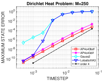
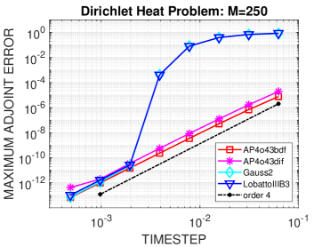
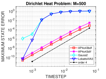
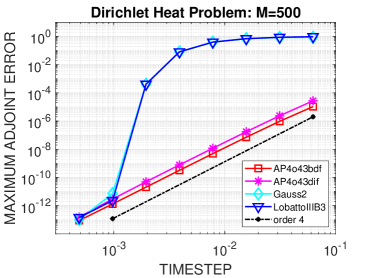
Figure 1: Dirichlet heat problem with $m=250,500$ spatial points and given exact control $u(t)$: $\|y(T)$$-$$y_{h}(T)\|_{\infty}$ (left) and $\|p(0)$$-$$p_{h}(0)\|_{\infty}$ (right).

3 Test case: Dirichlet boundary control problem

To illustrate an application of the derived expressions for the exact discrete solutions of the linear heat equation equipped with different boundary conditions, we consider the following ODE-constrained optimal control problem with an incorporated boundary control of Dirichlet type:

$$\min_{(y,u)}C \,:=\frac{1}{2}\|y(T)-\hat{y}\|^{2}_{2}+\frac{\alpha}{2}\int_{0}^{T}u(t)^{2}\,dt$$

$$\text{subject to }y^{\prime}(t) \,=My(t)+\gamma e_{m}u(t),\quad t\in(0,T],$$

$$y(0) \,=\mbox{1\hskip-2.40005ptl},$$

with $T\!=\!1$, $\gamma\!=\!2/\xi^{2}$, $\alpha\!=\!1$, $\mbox{1\hskip-2.40005ptl}=(1,\ldots,1)^{T}\in{\mathbb{R}}^{m}$, state vector $y(t)\in{\mathbb{R}}^{m}$, and $M$ as defined in (12) with $\theta\!=\!3$. We set $\delta_{1}\!=\!\delta_{2}\!=\!1/75$ in (34) and compute the target profile $\hat{y}\in{\mathbb{R}}^{m}$ from (35) with coefficients for $y(T)$ defined in (36).

We will compare numerical results for four time integrators of classical order four: the symmetric 2-stage Gauss method [3, Table II.1.1], the symmetric 3-stage partitioned Runge-Kutta pair Lobatto IIIA-IIIB [3, Table II.2.2] and our recently developed two-step Peer methods AP4o43bdf and AP4o43dif [5]. The two one-step methods are symplectic and therefore well suited for optimal control [3, 8].

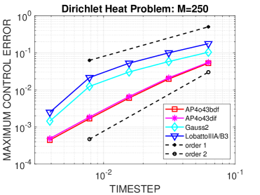
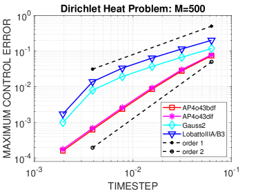
Figure 2: Dirichlet heat problem with $m=250,500$ spatial points, solved by gradient descent for $(y,p,u)$: $\max_{n,i}|u(t_{ni})$$-$$u_{h}(t_{ni})|$

Two test scenarios are considered. First, the accuracy of the numerical approximations for $y(T)$ and $p(0)$ are studied, where the exact control $u(t)=-\gamma p_{m}(t)/\alpha$ is used. The initial value for the multiplier is set to $p(T)=y_{h}(T)-\hat{y}$ with $y_{h}(T)$ being the approximation of $y(T)$ with time step $h$. In this case, the Karush-Kuhn-Tucker system decouples and only two systems of linear ODEs have to be solved. In the second scenario, the optimal control problem is solved for all unknowns $(y,p,u)$ by a gradient method with line search as implemented in the Matlab routine fmincon, see e.g. [1, 9] for more details, and the errors for the control are discussed. The control variable $u(t)$ is approximated at the nodes $t_{ni}\!=\!t_{n}+c_{i}h$, $i=1,\ldots,s,$ chosen by the time integrators on a time grid $\{t_{0},\ldots,t_{N}\}$ with step size $h$ and $s$ stages [2, 5]. In both test cases, we use $m\!=\!250$ and $m\!=\!500$ to also study the influence of the system size. The number of time steps are $N=2^{k}$ with $k=4,\ldots,11$.

In Fig. 1, results for the first test scenario are shown. Not surprisingly, the serious order reduction for the symplectic one-step Runge-Kutta methods are clearly seen. This phenomenon is well understood and occurs particularly drastically for time-dependent Dirichlet boundary conditions [7]. This drawback is shared by all one-step methods due to their insufficient stage order. Note that the number of affected time steps increases when the system size is doubled. In contrast, the newly designed two-step Peer methods for optimal control problems work quite close to their theoretical order four for the state $y$ and the adjoint $p$. The order reduction for the one-step methods is also visible for the more challenging fully coupled problem. The results plotted in Fig. 2 show a reduction to first order for the approximation of the control, whereas the two-step methods perform with order two for this problem. We refer to [2] for a discussion of the convergence order for general ODE constrained optimal control problems. Once again, the range of the affected time steps depends on the problem size. It increases for finer spatial discretizations.

References

• [1] J.T. Betts. Practical Methods for Optimal Control and Estimation Using Nonlinear Programming. SIAM, 2010.
• [2] W.W. Hager. Runge-Kutta methods in optimal control and the transformed adjoint system. Numer. Math., 87:247–282, 2000.
• [3] E. Hairer, Ch. Lubich, and G. Wanner. Geometric Numerical Integration, Structure-Preserving Algorithms for Ordinary Differential Equations, volume 31 of Springer Series in Computational Mathematics. Springer, Heidelberg, Berlin, 2006.
• [4] J. Lang and B.A. Schmitt. Discrete adjoint implicit peer methods in optimal control. J. Comput. Appl. Math., 416:114596, 2022.
• [5] J. Lang and B.A. Schmitt. Implicit A-stable peer triplets for ODE constrained optimal control problems. Algorithms, 15:310, 2022.
• [6] Ch. Lubich and A. Ostermann. Runge-Kutta approximation of quasi-linear parabolic equations. Math. Comp., 64:601–627, 1995.
• [7] A. Ostermann and M. Roche. Runge-Kutta methods for partial differential equations and fractional orders of convergence. Math. Comp., 59:403–420, 1992.
• [8] J.M. Sanz-Serna. Symplectic Runge–Kutta schemes for adjoint equations, automatic differentiation, optimal control, and more. SIAM Review, 58:3–33, 2016.
• [9] J.L. Troutman. Variational Calculus and Optimal Control. Springer, New York, 1996.