Laboratory-frame tests of quantum entanglement in $H\to WW$

Abstract

Quantum entanglement between the two $W$ bosons resulting from the decay of a Higgs boson may be investigated in the dilepton channel $H\to WW\to\ell\nu\ell\nu$ using laboratory-frame observables that only involve the charged leptons $\ell=e,\mu$. The dilepton invariant mass distribution, already measured by the ATLAS and CMS Collaborations at the LHC, can be used to observe the quantum entanglement of the $WW$ pair with a statistical sensitivity of $7\sigma$ with Run 2 data, and of $6\sigma$ when including theoretical systematics. As a by-product, the relation between $W$ rest frame (four-dimensional) angular distributions, $H\to WW$ decay amplitudes, and spin correlation coefficients, is written down.

I Introduction

Ten years after the discovery of the Higgs boson by the ATLAS and CMS experiments ATLAS:2012yve ; CMS:2012qbp , the statistics collected at the Large Hadron Collider (LHC) allows to test its properties in many production and decay modes ATLAS:2022vkf ; CMS:2022dwd . The main goal is to determine from experimental data whether the 125 GeV particle discovered corresponds to the Standard Model (SM) Higgs or not; in particular, whether it is the first discovered particle of an extended scalar sector. In addition, tests of the quantum properties of its decay, i.e. the quantum entanglement and possible violation of Bell inequalities Bell:1964kc are recently attracting attention Barr:2021zcp ; Aguilar-Saavedra:2022wam . While there is no experimental evidence to call into question the validity of quantum mechanics, testing it at the energy frontier is of high relevance. And the proposed tests often yield, as a by-product, new observables that might also be useful in searches for physics beyond the SM. Several studies in this regard have been performed for the entangled state of a top quark-antiquark pair Afik:2020onf ; Fabbrichesi:2021npl ; Severi:2021cnj ; Aoude:2022imd ; Afik:2022kwm ; Aguilar-Saavedra:2022uye ; Fabbrichesi:2022ovb ; Afik:2022dgh .

The decays $H\to VV$, $V=W,Z$ (with one of the weak bosons off shell) provide the ideal environment to test Higgs properties. In particular, quantum entanglement leaves its imprint in the spin correlation between the daughter weak bosons: because the Higgs is a spin-zero particle, the $VV$ pair is produced in a state of vanishing total angular momentum. If the $V$ were produced at rest in the Higgs rest frame, the orbital angular momentum would also vanish and the $VV$ pair would be in a maximally-entangled spin-singlet state. In practice, the two bosons are produced quite close to a spin singlet.

The possible violation of Bell-like inequalities in $H\to W^{+}W^{-}$ has been addressed in Ref. Barr:2021zcp , focusing on the dilepton final state $W^{+}W^{-}\to\ell^{+}\nu\ell^{-}\nu$, $\ell=e,\mu$, and using for spin measurements $W$-rest frame angular distributions. This implicitly assumes that the $W$ rest frames can be determined, which is not obvious because the two neutrinos are undetected, and only the sum of their transverse momenta can be identified with the missing transverse energy (MET) in the event. A reconstruction of the $W$ momenta using a kinematical fit or a multivariate method, e.g. a neural network, faces the difficulty of selecting a ‘best solution’ for the neutrino momenta within a two-dimensional manifold of possible solutions allowed by the kinematical constraints. The procedure adopted for the $W$ momenta determination might wash out the information from their spin that is transferred to the daughter leptons, but it may be worth exploring this kind of methods.

On the other hand, in this paper we propose tests of the $WW$ entanglement based on laboratory-frame observables, such as (i) the dilepton invariant mass $m_{\ell\ell}$; (ii) the angular separation between the leptons in the plane orthogonal to the beam axis $\phi_{\ell\ell}$; (iii) their pseudo-rapidity difference $\eta_{\ell\ell}$. We note that a similar approach was followed to establish the existence of spin correlations in $t\bar{t}$ production at the LHC. In the dilepton decay $t\bar{t}\to\ell^{+}\nu b\ell^{-}\nu b$, the azimuthal angle difference between the charged leptons in the laboratory frame was identified in Ref. Mahlon:2010gw to be quite sensitive to discriminate the SM versus the no-correlation scenario. Subsequently, this distribution was measured by the ATLAS ATLAS:2012ao and CMS CMS:2013roq Collaborations to establish the existence of spin correlations.

In order to investigate the feasibility of the entanglement measurement, in section II we use the helicity amplitude formalism of Jacob and Wick Jacob:1959at to write down the general prediction for polarisation and spin correlations in $H\to VV$, in terms of the decay amplitudes. In section III we discuss the $m_{\ell\ell}$, $\phi_{\ell\ell}$ and $\eta_{\ell\ell}$ distributions as a test of the $W^{+}W^{-}$ entanglement. The experimental prospects to disentangle the two options are examined in section IV, and our results are discussed in section V.

II $H\to VV$ and angular momentum

In order to be more general, let us consider the decay $H\to V_{1}V_{2}$, with $V_{1}V_{2}=ZZ,W^{+}W^{-}$ and label as $f=\ell,\nu$ the decay products of the weak bosons. Using the helicity amplitude formalism Jacob:1959at we can write the amplitudes for the decay $H\to V_{1}V_{2}\to f_{1}f_{1}^{\prime}f_{2}f_{2}^{\prime}$ as

$$A_{\lambda_{1}\lambda_{1}^{\prime}\lambda_{2}\lambda_{2}^{\prime}} = \sum_{\Lambda_{1}\Lambda_{2}}a_{\Lambda_{1}\Lambda_{2}}b_{\lambda_{1}\lambda_{1}^{\prime}}c_{\lambda_{2}\lambda_{2}^{\prime}}$$ (1)

$$\times D_{\Lambda_{1}\lambda}^{1*}(\phi_{1},\theta_{1},0)D_{\Lambda_{2}\lambda^{\prime}}^{1*}(\bar{\phi}_{2},\bar{\theta}_{2},0)$$

where $\Lambda_{1,2}$ are the helicities of $V_{1}$ and $V_{2}$, respectively, with $\Lambda_{1}=\Lambda_{2}$ by angular momentum conservation; $\lambda_{i}^{\scriptscriptstyle(^{\prime})}$ are the helicities of $f_{i}^{\scriptscriptstyle(^{\prime})}$, and $\lambda^{\scriptscriptstyle(^{\prime})}=\lambda_{1}^{\scriptscriptstyle(^{\prime})}-\lambda_{2}^{\scriptscriptstyle(^{\prime})}$. Note that the off-shell $V$ propagator includes a ‘scalar’ component that produces distinct terms in the angular distributions. However, when coupled to massless external fermions the scalar component vanishes; therefore, we can safely consider the off-shell $W$ as a spin-1 particle Groote:2012jq . In the above equation, the angular dependence is given by the well-known Wigner functions wigner

$$D^{j}_{m^{\prime}m}(\alpha,\beta,\gamma)\equiv\langle jm^{\prime}|e^{-i\alpha J_{z}}e^{-i\beta J_{y}}e^{-i\gamma J_{z}}|jm\rangle\,,$$ (2)

and $a_{\Lambda_{1}\Lambda_{2}}$, $b_{\lambda_{1}\lambda_{1}^{\prime}}$ and $c_{\lambda_{2}\lambda_{2}^{\prime}}$ are constants that depend on the helicity combination considered. For $Z$ bosons there are two non-zero combinations $(\lambda_{i},\lambda_{i}^{\prime})=(\pm 1/2,\mp 1/2)$, and the corresponding $b$ and $c$ constants are related by the ratio of the left- and right-handed couplings to leptons, $g_{R}^{\ell}\,:\,g_{L}^{\ell}$. For $W$ bosons there is only one such combination because the coupling is purely left-handed. The angles $(\theta_{1},\phi_{1})$ are the polar coordinates of the three-momentum of $f_{1}$ in the $V_{1}$ rest frame, and likewise the angles $(\bar{\theta}_{2},\bar{\phi}_{2})$ are the polar coordinates of the three-momentum of $f_{2}$ in the $V_{2}$ rest frame. Using

$$D^{j}_{m^{\prime}m}(\alpha,\beta,\gamma)=e^{-i\alpha m^{\prime}}e^{-i\gamma m}d^{j}_{m^{\prime}m}(\beta)$$ (3)

the amplitudes can be simplified to

$$A_{\lambda_{1}\lambda_{1}^{\prime}\lambda_{2}\lambda_{2}^{\prime}} = \sum_{\Lambda_{1}\Lambda_{2}}a_{\Lambda_{1}\Lambda_{2}}b_{\lambda_{1}\lambda_{1}^{\prime}}c_{\lambda_{2}\lambda_{2}^{\prime}}$$ (4)

$$\times e^{i\Lambda_{1}(\phi_{1}+\bar{\phi}_{2})}d_{\Lambda_{1}\lambda}^{1}(\theta_{1})d_{\Lambda_{2}\lambda^{\prime}}^{1}(\bar{\theta}_{2})\,.$$

The orientation of the three axes in the reference systems for the $V_{1,2}$ rest frames stems from the precise way in the helicity states are defined (see for example libro ). If we set a reference system $(x,y,z)$ in the Higgs rest frame, in which the $V_{1}$ boson three-momentum has angular coordinates $(\theta,\phi)$, the reference system $(x_{1},y_{1},z_{1})$ in the $V_{1}$ rest frame has the axes as follows:

• The $\hat{z}_{1}$ axis is in the direction of the $V_{1}$ boson three-momentum in the Higgs rest frame, $\hat{z}_{1}=\sin\theta\cos\phi\,\hat{x}+\sin\theta\sin\phi\,\hat{y}+\cos\theta\,\hat{z}$.

• The $\hat{y}_{1}$ axis is in the $xy$ plane, making an angle $\phi$ with the $\hat{y}$ axis: $\hat{y}_{1}=-\sin\phi\,\hat{x}+\cos\phi\,\hat{y}$.

• The $\hat{x}_{1}$ axis is orthogonal to both, $\hat{x}_{1}=\hat{y}_{1}\times\hat{z}_{1}=\cos\theta\cos\phi\,\hat{x}+\cos\theta\sin\phi\,\hat{y}-\sin\theta\hat{z}$.

For the reference system $(x_{2},y_{2},z_{2})$ in the $V_{2}$ rest frame one has a similar definition. However, for entanglement studies it is convenient to use the same definition of axes in both rest frames Aguilar-Saavedra:2022wam . A simple computation shows that

$$\hat{x}_{2}=\hat{x}_{1}\,,\quad\hat{y}_{2}=-\hat{y}_{1}\,,\quad\hat{z}_{2}=-\hat{z}_{1}\,,$$ (5)

therefore the polar coordinates of the $f_{2}$ three-momentum in the $V_{2}$ rest frame, with respect to the axes defined for the $V_{1}$ rest frame, are

$$\theta_{2}=\pi-\bar{\theta}_{2}\,,\quad\phi_{2}=-\bar{\phi}_{2}\,.$$ (6)

Using the symmetry properties of the $d_{m^{\prime}m}^{j}$ functions, the amplitudes (4) can be rewritten as

$$A_{\lambda_{1}\lambda_{1}^{\prime}\lambda_{2}\lambda_{2}^{\prime}} = \sum_{\Lambda_{1}\Lambda_{2}}a_{\Lambda_{1}\Lambda_{2}}b_{\lambda_{1}\lambda_{1}^{\prime}}c_{\lambda_{2}\lambda_{2}^{\prime}}$$ (7)

$$\times e^{i\Lambda_{1}(\phi_{1}-\phi_{2})}d_{\Lambda_{1}\lambda}^{1}(\theta_{1})d_{-\Lambda_{2}\lambda^{\prime}}^{1}(\theta_{2})\,.$$

The differential cross section is proportional to the squared amplitude summed over final state helicities,

$$\frac{d\sigma}{d\Omega_{1}d\Omega_{2}}\propto\sum_{\lambda_{1}\lambda_{1}^{\prime}\lambda_{2}\lambda_{2}^{\prime}}|A_{\lambda_{1}\lambda_{1}^{\prime}\lambda_{2}\lambda_{2}^{\prime}}|^{2}\,,$$ (8)

with $d\Omega_{i}=d\cos\theta_{i}d\phi_{i}$. Rather than writing the full expression, it is convenient to match it to a general parameterisation for the decay $V_{1}V_{2}\to f_{1}f_{1}^{\prime}f_{2}f_{2}^{\prime}$ in terms of polarisation and spin correlation coefficients.

A convenient parameterisation of the spin density operator for the $V_{1}V_{2}$ pair can be found in terms of the identity and 8 irreducible tensor operators $T^{L}_{M}$, with $L=1,2$ and $-L\leq M\leq L$, acting on the three-dimensional spin space for each boson Aguilar-Saavedra:2022wam . For convenience we normalise $T^{L}_{M}$ such that $\operatorname{Tr}\left[T^{L}_{M}\left(T^{L}_{M}\right)^{\dagger}\right]=3$, where $\left(T^{L}_{M}\right)^{\dagger}=(-1)^{M}\,T^{L}_{M}$ (note the change of normalisation with respect to Refs. Aguilar-Saavedra:2015yza ; Aguilar-Saavedra:2017zkn ). Specifically, the $T^{L}_{M}$ operators are defined as

$$T^{1}_{\pm 1}=\mp\frac{\sqrt{3}}{2}(S_{1}\pm iS_{2})\,,\quad T^{1}_{0}=\sqrt{\frac{3}{2}}S_{3}\,,$$

$$T^{2}_{\pm 2}=\frac{2}{\sqrt{3}}(T_{\pm 1}^{1})^{2}\,,\quad T^{2}_{\pm 1}=\sqrt{\frac{2}{3}}\left[T_{\pm 1}^{1}T_{0}^{1}+T_{0}^{1}T_{\pm 1}^{1}\right]\,,$$

$$T^{2}_{0}=\frac{\sqrt{2}}{3}\left[T_{1}^{1}T_{-1}^{1}+T_{-1}^{1}T_{1}^{1}+2(T_{0}^{1})^{2}\right]\,,$$ (9)

with $S_{i}$ the usual spin operators. In terms of these, the spin density operator reads Aguilar-Saavedra:2022wam

$$\rho = \frac{1}{9}\left[\mathbb{1}_{3}\otimes\mathbb{1}_{3}+A^{1}_{LM}\,T^{L}_{M}\otimes\mathbb{1}_{3}+A^{2}_{LM}\,\mathbb{1}_{3}\otimes T^{L}_{M}\right.$$ (10)

$$\left.+C_{L_{1}M_{1}L_{2}M_{2}}\,T^{L_{1}}_{M_{1}}\otimes T^{L_{2}}_{M_{2}}\right]\,,$$

where an implicit sum over all indices is understood. The coefficients satisfy the relations

$$(A^{1,2}_{LM})^{*}=(-1)^{M}\,A^{1,2}_{L\;-M}\,,$$

$$(C_{L_{1}M_{1}L_{2}M_{2}})^{*}=(-1)^{M_{1}+M_{2}}\,C_{L_{1}\;-M_{1}L_{2}\;-M_{2}}\,.$$ (11)

The angular distribution corresponding to this density operator can be compactly written Aguilar-Saavedra:2022wam in terms of spherical harmonics $Y_{\ell}^{m}$,

$$\frac{1}{\sigma}\frac{d\sigma}{d\Omega_{1}d\Omega_{2}}=\frac{1}{(4\pi)^{2}}\left[1+A_{LM}^{1}B_{L}Y_{L}^{M}(\theta_{1},\phi_{1})\right.$$

$$\quad+A_{LM}^{2}B_{L}Y_{L}^{M}(\theta_{2},\phi_{2})$$

$$\quad\left.+C_{L_{1}M_{1}L_{2}M_{2}}B_{L_{1}}B_{L_{2}}Y_{L_{1}}^{M_{1}}(\theta_{1},\phi_{1})Y_{L_{2}}^{M_{2}}(\theta_{2},\phi_{2})\right]\,,$$ (12)

with $B_{1}$, $B_{2}$ constants. For $V_{1}=V_{2}=Z$, and taking $f_{1,2}$ as the negative leptons, one has

$$B_{1}=-\sqrt{2\pi}\eta_{\ell}\ ,\ \ \ B_{2}=\sqrt{\frac{2\pi}{5}}$$ (13)

with Aguilar-Saavedra:2017zkn

$$\eta_{\ell}=\frac{(g_{L}^{\ell})^{2}-(g_{R}^{\ell})^{2}}{(g_{L}^{\ell})^{2}+(g_{R}^{\ell})^{2}}=\frac{1-4s_{W}^{2}}{1-4s_{W}^{2}+8s_{W}^{4}}\simeq 0.13\,,$$ (14)

$s_{W}$ being the sine of the weak mixing angle. For $V_{2}=W^{-}$, and taking $f_{2}$ as the negative lepton, $B_{1,2}$ are as in (13) setting $\eta_{\ell}=1$. For $V_{1}=W^{+}$, and taking $f_{1}$ as the positive lepton (which is an anti-fermion), $B_{1,2}$ are as in (13) but setting instead $\eta_{\ell}=-1$. Thus the parameterisation (12) with the above conventions summarises the double distribution for both $ZZ$ and $W^{+}W^{-}$ in terms of polarisation and spin correlation coefficients.

One can match the expression (12) to (8) properly normalised, to identify the non-zero coefficients. Let us define

$$\mathcal{N}=|a_{11}|^{2}+|a_{00}|^{2}+|a_{{\textstyle\scriptscriptstyle-}1{\textstyle\scriptscriptstyle-}1}|^{2}\,.$$ (15)

Within the SM, CP is conserved in the $H\to V_{1}V_{2}$ decay at the leading order (LO), and only

$$A_{20}^{1}=A_{20}^{2}=\frac{1}{\sqrt{2}}\frac{1}{\mathcal{N}}\left[|a_{11}|^{2}+|a_{{\textstyle\scriptscriptstyle-}1{\textstyle\scriptscriptstyle-}1}|^{2}-2|a_{00}|^{2}\right]\,,$$

$$C_{1010}=-\frac{3}{2}\frac{1}{\mathcal{N}}\left[|a_{11}|^{2}+|a_{{\textstyle\scriptscriptstyle-}1{\textstyle\scriptscriptstyle-}1}|^{2}\right]\,,$$

$$C_{2020}=\frac{1}{2}\frac{1}{\mathcal{N}}\left[|a_{11}|^{2}+|a_{{\textstyle\scriptscriptstyle-}1{\textstyle\scriptscriptstyle-}1}|^{2}+4|a_{00}|^{2}\right]\,,$$

$$C_{222{\textstyle\scriptscriptstyle-}2}=C_{2{\textstyle\scriptscriptstyle-}222}^{*}=3\frac{1}{\mathcal{N}}\;a_{11}a_{{\textstyle\scriptscriptstyle-}1{\textstyle\scriptscriptstyle-}1}^{*}\,,$$

$$C_{111{\textstyle\scriptscriptstyle-}1}=-C_{212{\textstyle\scriptscriptstyle-}1}=C_{1{\textstyle\scriptscriptstyle-}111}^{*}=-C_{2{\textstyle\scriptscriptstyle-}121}^{*}$$

$$\quad=-\frac{3}{2}\frac{1}{\mathcal{N}}\left[a_{11}a_{00}^{*}+a_{00}a_{{\textstyle\scriptscriptstyle-}1{\textstyle\scriptscriptstyle-}1}^{*}\right]$$ (16)

are non-vanishing. CP-violating effects in the SM arise beyond the LO but are at the level of $10^{-5}$ Gritsan:2022php , so CP conservation is an excellent approximation. If CP is broken in the $H\to V_{1}V_{2}$ decay due to effects beyond the SM, additional terms appear

$$A_{10}^{1}=-A_{10}^{2}=\sqrt{\frac{3}{2}}\frac{1}{\mathcal{N}}\left[|a_{11}|^{2}-|a_{{\textstyle\scriptscriptstyle-}1{\textstyle\scriptscriptstyle-}1}|^{2}\right]\,,$$

$$C_{1020}=-C_{2010}=\frac{\sqrt{3}}{2}\frac{1}{\mathcal{N}}\left[|a_{11}|^{2}-|a_{{\textstyle\scriptscriptstyle-}1{\textstyle\scriptscriptstyle-}1}|^{2}\right]\,,$$

$$C_{1{\textstyle\scriptscriptstyle-}121}=-C_{2{\textstyle\scriptscriptstyle-}111}=C_{112{\textstyle\scriptscriptstyle-}1}^{*}=-C_{211{\textstyle\scriptscriptstyle-}1}^{*}$$

$$\quad=\frac{3}{2}\frac{1}{\mathcal{N}}\left[a_{00}a_{11}^{*}-a_{{\textstyle\scriptscriptstyle-}1{\textstyle\scriptscriptstyle-}1}a_{00}^{*}\right]\,.$$ (17)

III Entanglement in the laboratory frame

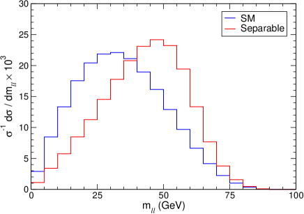
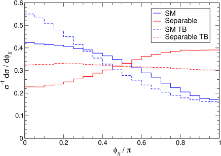
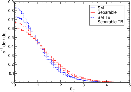
Figure 1: Dilepton observables: invariant mass (top), azimuthal angle difference (middle) and pseudo-rapidity difference (bottom). The dashed lines labeled as ‘TB’ show the distributions with $p_{T}^{H}=20$ GeV.

From now on we focus on the decay $H\to W^{+}W^{-}$. Reference Aguilar-Saavedra:2022wam showed that a necessary and sufficient condition for entanglement (which applies too to this decay) is $C_{222{\textstyle\scriptscriptstyle-}2}\neq 0$. Since $a_{11}=a_{{\textstyle\scriptscriptstyle-}1{\textstyle\scriptscriptstyle-}1}$, Eq. (16) implies that the $W^{+}W^{-}$ pair is entangled as long as these amplitudes are non-vanishing. The test of entanglement then consists in comparing between (i) the SM; (ii) a decay where the $W$ bosons have longitudinal polarisation, $a_{11}=a_{{\textstyle\scriptscriptstyle-}1{\textstyle\scriptscriptstyle-}1}=0$, $a_{00}\neq 0$.

We generate a sample of $H\to W^{+}W^{-}\to e^{\pm}\nu\mu^{\mp}\nu$ at the LO in the SM using MadGraph Alwall:2014hca , with the implementation of the $gg\to H$ loop as a contact interaction. A second sample is obtained from the former by modifying both $W$ decays following the CAR method Aguilar-Saavedra:2022kgy so that the angular distributions of the decay products correspond to zero helicity. This modification of the decay gives the exact result for polarised $H\to W^{+}W^{-}$ decays, because the kinematics of the $WW$ pair in the Higgs rest frame is independent of the polarisation.

For the two cases (SM versus longitudinal $W$ polarisations) Fig. 1 shows the distributions of the three variables of interest: (i) the dilepton invariant mass; (ii) the angle $\phi_{\ell\ell}$ between the two leptons in the plane transverse to the beam axis; (iii) the modulus of the pseudo-rapidity difference $\eta_{\ell\ell}=|\eta_{\ell^{+}}-\eta_{\ell^{-}}|$. The difference in the $\phi_{\ell\ell}$ distributions between the two possibilities is striking and is caused by the two charged leptons being preferably emitted in the same direction when the $W^{+}W^{-}$ pair has like helicities. However, this variable is quite sensitive to boosts in the transverse direction due to initial state radiation, which causes the Higgs boson to be produced with non-zero transverse momentum $p_{T}^{H}$. We illustrate this effect by applying a boost in the transverse plane that gives $p_{T}^{H}=20$ GeV. The resulting distributions are shown in dashed lines. The modifications in $\eta_{\ell\ell}$ and especially $\phi_{\ell\ell}$ are important but one can see that the differences between the SM and the separable case are maintained at this level. Note that $m_{\ell\ell}$ is Lorentz invariant and therefore is unaffected by non-zero $p_{T}^{H}$, and it can also be measured in the laboratory frame.

IV Sensitivity to entanglement

In contrast to the $H\to ZZ$ decay mode studied in Ref. Aguilar-Saavedra:2022wam , the background for $H\to WW$ is much larger than this signal. This has two consequences that may jeopardise the observation of entanglement. First, the kinematical selection necessary to suppress the background may shape the $H$ signal and dilute the differences between the SM and separable case. Second, the statistical uncertainties in the background, larger than the signal, make it harder (and statistically less significant) the discrimination between the two hypotheses.

For the sensitivity estimation we restrict ourselves to the different-flavour final state, $H\to WW\to e^{\pm}\nu\mu^{\mp}\nu$, for which the background is much smaller, and dominated by electroweak $WW$ production when both charged leptons are energetic CMS:2022uhn . The $H\to WW\to e^{\pm}\nu\mu^{\mp}\nu$ processes are generated as described in the previous section, with a Monte Carlo statistics of $2\times 10^{6}$ events. For the background $pp\to WW\to e^{\pm}\nu\mu^{\mp}\nu$ we also use MadGraph at the LO, with a Monte Carlo statistics of $3\times 10^{6}$ events. The parton-level event samples are showered and hadronised with Pythia 8.3 Sjostrand:2007gs and a fast detector simulation is performed with Delphes deFavereau:2013fsa , using the default CMS card.

Despite the Monte Carlo generation is done at the LO, we use higher-order predictions of the cross sections to calculate the expected number of events. The Higgs cross section in gluon-gluon fusion at next-to-next-to-next-to-leading order is 48.61 pb at a centre-of-mass energy of 13 TeV Cepeda:2019klc , and the Higgs branching ratio decay into $e^{\pm}\nu\mu^{\mp}\nu$ is $5.038\times 10^{-3}$ Cepeda:2019klc , yielding an overall cross section times branching ratio of 245 fb at 13 TeV. The $WW$ cross section is normalised to next-to-next-to-leading order (NNLO) with a $K$-factor of 1.4 Grazzini:2019jkl , and for the final state considered is 2.6 pb.

We follow Ref. CMS:2022uhn to implement a kinematical selection on charged leptons:

• Both leptons must have pseudo-rapidities $|\eta|\leq 2.5$, the leading one with transverse momentum $p_{T}\geq 25$ GeV and the sub-leading one with $p_{T}\geq 20$ GeV.

• The transverse momentum and invariant mass of the dilepton pair must be above the minimum thresholds $p_{T}^{\ell\ell}\geq 30$ GeV, $m_{\ell\ell}\geq 12$ GeV, respectively, and the missing energy $\mbox{$\raisebox{1.29167pt}{$\not$}E_{T}$}\geq 20$ GeV.

• The transverse mass of the event (with the usual definition) must be $m_{T}\geq 60$ GeV; the transverse mass constructed using only the sub-leading lepton (see Ref. CMS:2022uhn for the precise definition) is $m_{T2}\geq 30$ GeV.

With this selection, the electroweak $WW$ background is dominant CMS:2022uhn ; therefore, we can safely ignore the rest of them, mainly $t\bar{t}$ and $tW$, to obtain a realistic estimate of the statistical sensitivity to quantum entanglement.

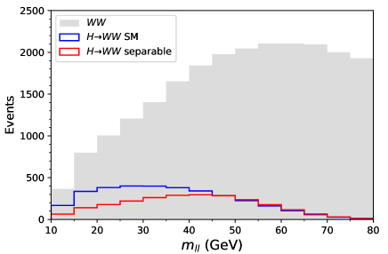
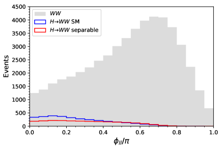
Figure 2: Dilepton observables: dilepton invariant mass (top) and azimuthal angle difference (bottom).

We present in Fig. 2 the kinematical distributions for $m_{\ell\ell}$ (top) and $\phi_{\ell\ell}$ (bottom) after simulation, for $H\to WW$ in the SM and the separable case, as well as for the $WW$ background. The luminosity is taken as $L=138~{}\text{fb}^{-1}$. The differences in the shape of the $m_{\ell\ell}$ distribution observed at the parton level are maintained to a large extent. Moreover, the different angular distribution of the charged leptons leads to different event selection efficiencies (0.097 for the SM and 0.070 for the separable case) which also contribute to the discrimination between the two hypotheses. The striking differences in the shape of the $\phi_{\ell\ell}$ distribution that were observed at the parton level are washed out by the event selection, especially by the requirements on transverse masses. The $\eta_{\ell\ell}$ distribution turns out to be uninteresting because the SM and separable hypotheses are quite alike, and the signal concentrates near $\eta_{\ell\ell}\sim 0$ where the $WW$ background is also largest.

For the calculation of the expected statistical significance of the SM hypothesis over the separability we calculate the expected $\chi^{2}$ for the $WW+H$ (SM) versus the $WW+H$ (separable) hypotheses, using the ranges of $m_{\ell\ell}$ and $\phi_{\ell\ell}$ shown in Fig. 2. This is a conservative approach since a narrower range would give larger deviations; on the other hand, the obtained estimation is more robust and less sensitive to the binning choice and possible mismeasurements of $m_{\ell\ell}$ and $\phi_{\ell\ell}$. For the $m_{\ell\ell}$ distribution we obtain $\chi^{2}=145$ for 14 degrees of freedom (d.o.f.) which amounts to a $7.1\sigma$ significance. (Selecting the range $10~{}\text{GeV}\leq m_{\ell\ell}\leq 40~{}\text{GeV}$ the statistical significance raises to $7.8\sigma$.) For the $\phi_{\ell\ell}$ distribution we obtain $\chi^{2}=76$ for 20 d.o.f., which amounts to $4\sigma$.

The question that immediately arises is how systematic uncertainties may affect these estimates. In this regard, the theoretical predictions for all processes are known at least to NNLO accuracy. The Higgs total production cross section can also be directly measured in other decay channels such as $H\to ZZ$. The normalisation for the background, from $WW$ and other processes, can be fixed by using different kinematical regions (see for example Ref. CMS:2022uhn ), with scale factors that are close to unity. Shape uncertainties have to be considered as well.

We have investigated the effect of theoretical shape uncertainties in the $m_{\ell\ell}$ distribution. The signal distribution is quite robust, as the dilepton invariant mass from the on-shell Higgs decay is determined by the decay kinematics. On the other hand, uncertainties in the $WW$ background may affect the signal extraction. We have investigated the uncertainty associated to:

• Changing the factorisation and renormalisation scale from the total transverse mass $M_{T}$ (default) to $M_{T}/2$ and $2M_{T}$.

• Replacing the baseline NNPDF 3.1 NNPDF:2017mvq parton density functions (PDFs) by MMHT 2014 Harland-Lang:2014zoa .

All the alternative $WW$ samples are generated with $3\times 10^{6}$ events. We present in Fig. 3 the distribution for the $WW$ background in the relevant region $m_{\ell\ell}\leq 80$ GeV. The relative size of the samples has been normalised to the same cross section in the sideband $m_{\ell\ell}\in[80,150]$ GeV.

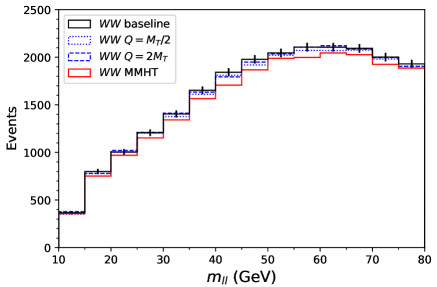
Figure 3: Dilepton invariant mass for the $WW$ background: baseline prediction and with different scales or PDFs. The vertical bars represent the statistical uncertainty for 138 fb^-1.

In the most relevant region of small $m_{\ell\ell}$ (where the SM and separable cases are better discriminated, see Fig. 2) the theoretical uncertainties are small, of the order of the statistical uncertainty. Therefore, it is expected that theoretical uncertainties do not spoil the discrimination between the two hypotheses. We calculate the resulting $p$-value by using a Bayesian approach Demortier:1099967 , assuming a flat prior for the different SM predictions. With the inclusion of the above discussed uncertainties, the $p$-value for the comparison between the SM and separable hypotheses slightly drops to $6.1$ standard deviations. An estimation of experimental systematic uncertainties can only be done with a full detector simulation and is beyond the scope of this work.

V Discussion

Generically, the test of quantum properties such and entanglement and violation of Bell inequalities requires the measurement of spin correlation observables. This, in turn, requires the reconstruction of rest frames and thus the full reconstruction of the relevant event kinematics. For example, the measurement of the $C_{L_{1}M_{1}L_{2}M_{2}}$ coefficients in (12) can be done by integration with spherical harmonics, which in turn requires knowledge of the angles $\theta_{i}$ and $\phi_{i}$ in the respective $V_{i}$ rest frames. For the decay $H\to ZZ\to 4\ell$ Aguilar-Saavedra:2022wam this is not a problem, but for $H\to WW\to\ell^{+}\nu\ell^{-}\nu$ the presence of the two neutrinos makes a unique reconstruction of the kinematics simply not possible. A probabilistic approach using a kinematical fit or a multivariate method remains to be explored.

Still, in the particular case of $H\to V_{1}V_{2}$ decays there is a unique characterisation of the entanglement: as we have shown in section II, the separability condition $C_{222-2}=0$ Aguilar-Saavedra:2022wam implies that only one of the three decay amplitudes, namely with both bosons longitudinally polarised, is non-zero. Thus, we can reformulate the entanglement condition as a binary test: SM versus longitudinal polarisation. And this binary test can be performed using laboratory-frame observables, as shown in section III. For the specific case of the dilepton invariant mass, which is a quite robust variable already measured by the ATLAS and CMS Collaborations, the expected significance between the two hypotheses is of $6.1\sigma$ with a luminosity of 138 fb^-1. This figure includes statistical uncertainties, as well as an estimation of shape systematics from modelling. Therefore, the entanglement in $H\to WW$ could be established with the already collected Run 2 data.

References

- (1) ATLAS Collaboration, G. Aad et al., “Observation of a new particle in the search for the Standard Model Higgs boson with the ATLAS detector at the LHC,” Phys. Lett. B 716 (2012) 1–29, arXiv:1207.7214 [hep-ex].
- (2) CMS Collaboration, S. Chatrchyan et al., “Observation of a New Boson at a Mass of 125 GeV with the CMS Experiment at the LHC,” Phys. Lett. B 716 (2012) 30–61, arXiv:1207.7235 [hep-ex].
- (3) ATLAS Collaboration, “A detailed map of Higgs boson interactions by the ATLAS experiment ten years after the discovery,” Nature 607 no. 7917, (2022) 52–59, arXiv:2207.00092 [hep-ex].
- (4) CMS Collaboration, “A portrait of the Higgs boson by the CMS experiment ten years after the discovery,” Nature 607 no. 7917, (2022) 60–68, arXiv:2207.00043 [hep-ex].
- (5) J. S. Bell, “On the Einstein-Podolsky-Rosen paradox,” Physics Physique Fizika 1 (1964) 195–200.
- (6) A. J. Barr, “Testing Bell inequalities in Higgs boson decays,” Phys. Lett. B 825 (2022) 136866, arXiv:2106.01377 [hep-ph].
- (7) J. A. Aguilar-Saavedra, A. Bernal, J. A. Casas, and J. M. Moreno, “Testing entanglement and Bell inequalities in ,” arXiv:2209.13441 [hep-ph].
- (8) Y. Afik and J. R. M. de Nova, “Entanglement and quantum tomography with top quarks at the LHC,” Eur. Phys. J. Plus 136 no. 9, (2021) 907, arXiv:2003.02280 [quant-ph].
- (9) M. Fabbrichesi, R. Floreanini, and G. Panizzo, “Testing Bell Inequalities at the LHC with Top-Quark Pairs,” Phys. Rev. Lett. 127 no. 16, (2021) 161801, arXiv:2102.11883 [hep-ph].
- (10) C. Severi, C. D. E. Boschi, F. Maltoni, and M. Sioli, “Quantum tops at the LHC: from entanglement to Bell inequalities,” Eur. Phys. J. C 82 no. 4, (2022) 285, arXiv:2110.10112 [hep-ph].
- (11) R. Aoude, E. Madge, F. Maltoni, and L. Mantani, “Quantum SMEFT tomography: top quark pair production at the LHC,” arXiv:2203.05619 [hep-ph].
- (12) Y. Afik and J. R. M. de Nova, “Quantum information with top quarks in QCD production,” arXiv:2203.05582 [quant-ph].
- (13) J. A. Aguilar-Saavedra and J. A. Casas, “Improved tests of entanglement and Bell inequalities with LHC tops,” arXiv:2205.00542 [hep-ph].
- (14) M. Fabbrichesi, R. Floreanini, and E. Gabrielli, “Constraining new physics in entangled two-qubit systems: top-quark, tau-lepton and photon pairs,” arXiv:2208.11723 [hep-ph].
- (15) Y. Afik and J. R. M. n. de Nova, “Quantum discord and steering in top quarks at the LHC,” arXiv:2209.03969 [quant-ph].
- (16) G. Mahlon and S. J. Parke, “Spin Correlation Effects in Top Quark Pair Production at the LHC,” Phys. Rev. D 81 (2010) 074024, arXiv:1001.3422 [hep-ph].
- (17) ATLAS Collaboration, G. Aad et al., “Observation of spin correlation in events from pp collisions at sqrt(s) = 7 TeV using the ATLAS detector,” Phys. Rev. Lett. 108 (2012) 212001, arXiv:1203.4081 [hep-ex].
- (18) CMS Collaboration, S. Chatrchyan et al., “Measurements of Spin Correlations and Top-Quark Polarization Using Dilepton Final States in Collisions at = 7 TeV,” Phys. Rev. Lett. 112 no. 18, (2014) 182001, arXiv:1311.3924 [hep-ex].
- (19) M. Jacob and G. C. Wick, “On the General Theory of Collisions for Particles with Spin,” Annals Phys. 7 (1959) 404–428.
- (20) S. Groote, J. G. Korner, and A. A. Pivovarov, “Understanding PT results for decays of leptons into hadrons,” Phys. Part. Nucl. 44 (2013) 285–298, arXiv:1212.5346 [hep-ph].
- (21) E. P. Wigner, Group Theory and Its Application to the Quantum Mechanics of Atomic Spectra. Academic Press, New York, 1959.
- (22) J. A. Aguilar-Saavedra, Helicity formalism and applications. Godel, Granada, Spain, 2015.
- (23) J. A. Aguilar-Saavedra and J. Bernabeu, “Breaking down the entire boson spin observables from its decay,” Phys. Rev. D 93 no. 1, (2016) 011301, arXiv:1508.04592 [hep-ph].
- (24) J. A. Aguilar-Saavedra, J. Bernabéu, V. A. Mitsou, and A. Segarra, “The boson spin observables as messengers of new physics,” Eur. Phys. J. C 77 no. 4, (2017) 234, arXiv:1701.03115 [hep-ph].
- (25) A. V. Gritsan et al., “Snowmass White Paper: Prospects of CP-violation measurements with the Higgs boson at future experiments,” arXiv:2205.07715 [hep-ex].
- (26) J. Alwall, R. Frederix, S. Frixione, V. Hirschi, F. Maltoni, O. Mattelaer, H. S. Shao, T. Stelzer, P. Torrielli, and M. Zaro, “The automated computation of tree-level and next-to-leading order differential cross sections, and their matching to parton shower simulations,” JHEP 07 (2014) 079, arXiv:1405.0301 [hep-ph].
- (27) J. A. Aguilar-Saavedra, “Crafting polarisations for top, and ,” arXiv:2208.00424 [hep-ph].
- (28) CMS Collaboration, “Measurements of the Higgs boson production cross section and couplings in the W boson pair decay channel in proton-proton collisions at = 13 TeV,” arXiv:2206.09466 [hep-ex].
- (29) T. Sjostrand, S. Mrenna, and P. Z. Skands, “A Brief Introduction to PYTHIA 8.1,” Comput. Phys. Commun. 178 (2008) 852–867, arXiv:0710.3820 [hep-ph].
- (30) DELPHES 3 Collaboration, J. de Favereau, C. Delaere, P. Demin, A. Giammanco, V. Lemaître, A. Mertens, and M. Selvaggi, “DELPHES 3, A modular framework for fast simulation of a generic collider experiment,” JHEP 02 (2014) 057, arXiv:1307.6346 [hep-ex].
- (31) M. Cepeda et al., “Report from Working Group 2: Higgs Physics at the HL-LHC and HE-LHC,” CERN Yellow Rep. Monogr. 7 (2019) 221–584, arXiv:1902.00134 [hep-ph].
- (32) M. Grazzini, S. Kallweit, J. M. Lindert, S. Pozzorini, and M. Wiesemann, “NNLO QCD + NLO EW with Matrix+OpenLoops: precise predictions for vector-boson pair production,” JHEP 02 (2020) 087, arXiv:1912.00068 [hep-ph].
- (33) NNPDF Collaboration, R. D. Ball et al., “Parton distributions from high-precision collider data,” Eur. Phys. J. C 77 no. 10, (2017) 663, arXiv:1706.00428 [hep-ph].
- (34) L. A. Harland-Lang, A. D. Martin, P. Motylinski, and R. S. Thorne, “Parton distributions in the LHC era: MMHT 2014 PDFs,” Eur. Phys. J. C 75 no. 5, (2015) 204, arXiv:1412.3989 [hep-ph].
- (35) L. Demortier, “P Values and Nuisance Parameters,”. https://cds.cern.ch/record/1099967.