Funnel-based Reachability Control of Unknown Nonlinear Systems
using Gaussian Processes

Sandeep Gorantla1,†, Jeel Chatrola1,†, Jay Bhagiya1,†, Adnane Saoud2, and Pushpak Jagtap1 *This work was supported in part by the Google Research Grant, the CSR Grant by Nokia Corporation, the SERB Start-up Research Grant, and by ANR PIA funding: ANR-20-IDEES-0002. The authors contributed equally.1S. Gorantla, J. Chatrola, J. Bhagiya, and P. Jagtap are with the Robert Bosch Center for Cyber-Physical Systems, Indian Institute of Science, Bangalore, India.{sgorantla,pushpak,jeelchatrola,jaybhagiya}@iisc.ac.in2Adnane Saoud is with Laboratoire des Signaux et Systèmes, CentraleSupélec, Université Paris Saclay, Gif-sur-Yvette, France. adnane.saoud@centralesupelec.fr
Abstract

This paper aims to synthesize a reachability controller for an unknown dynamical system. We first learn the unknown system using Gaussian processes and the (probabilistic) guarantee on the learned model. Then we use the funnel-based controller synthesis approach using this approximated dynamical system to design the controller for a reachability specification. Finally, the merits of the proposed method are shown using a numerical example.

I INTRODUCTION

Existing controller synthesis approaches generally rely on a mathematical model of the system, such as physics-based first principal models. The formal guarantees provided by the synthesized controller are valid as long as the considered dynamical model is accurate. When dealing with complex dynamical systems, describing the system in a closed-form model is often complicated. In this case, a common practice is to resort to data-driven techniques.

The Gaussian process is a non-parametric learning-based approach that provides probabilistic approach to approximate and to synthesize controllers for unknown systems [1]. There are several works that utilize GPs for providing MPC scheme [2], adaptive control [3], tracking control[4], backstepping control [5], feedback linearization [6], safe optimization of controller [7], reinforcement learning [8], and control barrier functions for safety specification [9].

This work will consider the controller synthesis problem for reachability specification for unknown dynamical systems. In the past few decades, there have been several works in the literature addressing reachability problem (see [10, 11, 12, 13, 14]) for known dynamical systems. To solve this problem, we leverage the funnel-based control approaches [15] that have been extensively used for controlling systems with prescribed performance constraints (see [16] and references therein for examples). We first employ the Gaussian process learning to approximate the system dynamics using the noisy measurements along a probabilistic bound on approximation. Then, the synthesis of a closed-form funnel-based control law that ensures the satisfaction of the reachability specification, with a given confidence, using the learned dynamics from the GP model, is presented. Finally, we show the validness of our approach using a numerical example.

The organization of the paper is as follows. Section II introduces some notations and present the main problem addressed in the paper. Section III explains how Gaussian processes make it possible to learn unknown dynamical systems along with statistical guarantees. Section IV presents a solution to the reachability problem by combining learned Gaussian processes with funnel-based control techniques. Finally, Section V presents numerical results validating the merits of the proposed approach.

II PROBLEM FORMULATION

II-A Notations

The set of real, positive real, nonnegative real, and positive integer numbers are represented using \mathbb{R}, +superscript\mathbb{R}^{+}, 0+superscriptsubscript0\mathbb{R}_{0}^{+}, and \mathbb{N}, respectively. psuperscript𝑝\mathbb{R}^{p} denotes p𝑝p-dimensional Euclidean space and p×qsuperscript𝑝𝑞\mathbb{R}^{p\times q} denotes a space of real matrices with p𝑝p rows and q𝑞q columns. A diagonal matrix in p×psuperscript𝑝𝑝{\mathbb{R}}^{p\times p} with diagonal entries d1,,dpsubscript𝑑1subscript𝑑𝑝d_{1},\ldots,d_{p} is denoted by diag{d1,,dp}𝑑𝑖𝑎𝑔subscript𝑑1subscript𝑑𝑝diag\{d_{1},\ldots,d_{p}\}. Given a matrix Mp×q𝑀superscript𝑝𝑞M\in{\mathbb{R}}^{p\times q}, MTsuperscript𝑀𝑇M^{T} represents transpose of matrix M𝑀M. For a vector x=[x1,,xn]Tn𝑥superscriptsubscript𝑥1subscript𝑥𝑛𝑇superscript𝑛x=[x_{1},\ldots,x_{n}]^{T}\in{\mathbb{R}}^{n}, we denote 𝗌𝗂𝗀𝗇(x)=[𝗌𝗂𝗀𝗇(x1),,𝗌𝗂𝗀𝗇(xn)]T𝗌𝗂𝗀𝗇𝑥superscript𝗌𝗂𝗀𝗇subscript𝑥1𝗌𝗂𝗀𝗇subscript𝑥𝑛𝑇\mathsf{sign}(x)=[\mathsf{sign}(x_{1}),\ldots,\mathsf{sign}(x_{n})]^{T}, where 𝗌𝗂𝗀𝗇(xi)={1if xi<01if xi0\mathsf{sign}(x_{i})=\left\{\begin{matrix}-1&\text{if }x_{i}<0\\ 1&\text{if }x_{i}\geq 0\end{matrix}\right., we use xnorm𝑥\|x\| and xsubscriptnorm𝑥\|x\|_{\infty} to denote Euclidean norm and infinity norm of a vector, respectively. We denote the empty set by \emptyset. We use 𝑰psubscript𝑰𝑝\bm{I}_{p} to represent the identity matrix in p×psuperscript𝑝𝑝{\mathbb{R}}^{p\times p}. For a,b𝑎𝑏a,b\in{\mathbb{R}} and a<b𝑎𝑏a<b, we use (a,b)𝑎𝑏(a,b) and [a,b]𝑎𝑏[a,b] to represent open and close intervals in {\mathbb{R}}, respectively. For a function f:pp:𝑓superscript𝑝superscript𝑝f:\mathbb{R}^{p}\rightarrow\mathbb{R}^{p}, fi:p:subscript𝑓𝑖superscript𝑝f_{i}:\mathbb{R}^{p}\rightarrow\mathbb{R}, i{1,2,,p}𝑖12𝑝i\in\{1,2,\ldots,p\} denotes the i𝑖i-th component of f𝑓f. Consider a set Xapsubscript𝑋𝑎superscript𝑝X_{a}\subset{\mathbb{R}}^{p}, its projection on i𝑖ith dimension, where i{1,,p}𝑖1𝑝i\in\{1,\ldots,p\}, is given by an interval [X¯ai,X¯ai]subscript¯𝑋𝑎𝑖subscript¯𝑋𝑎𝑖[\underline{X}_{ai},\overline{X}_{ai}]\subset{\mathbb{R}}, where X¯ai:=min{xi[x1,x2,,xp]Xa}assignsubscript¯𝑋𝑎𝑖subscript𝑥𝑖conditionalsubscript𝑥1subscript𝑥2subscript𝑥𝑝subscript𝑋𝑎\underline{X}_{ai}:=\min\{x_{i}\in{\mathbb{R}}\mid[x_{1},x_{2},\ldots,x_{p}]\in X_{a}\}, X¯ai:=max{xi[x1,x2,,xp]Xa}assignsubscript¯𝑋𝑎𝑖subscript𝑥𝑖conditionalsubscript𝑥1subscript𝑥2subscript𝑥𝑝subscript𝑋𝑎\overline{X}_{ai}:=\max\{x_{i}\in{\mathbb{R}}\mid[x_{1},x_{2},\ldots,x_{p}]\in X_{a}\}, and Int(Xa)Intsubscript𝑋𝑎\text{Int}(X_{a}) denotes interior of set Xasubscript𝑋𝑎X_{a}. 𝒩(m,C)𝒩𝑚𝐶\mathcal{N}(m,C) denotes multivariate Gaussian distribution, where mp𝑚superscript𝑝m\in{\mathbb{R}}^{p} and Cp×p𝐶superscript𝑝𝑝C\in{\mathbb{R}}^{p\times p} are mean and covariance matrices of appropriate sizes, respectively. For events B1,,Bpsubscript𝐵1subscript𝐵𝑝B_{1},\ldots,B_{p}, i=1pBisuperscriptsubscript𝑖1𝑝subscript𝐵𝑖\bigcap_{i=1}^{p}B_{i} represents inner product of events.

II-B Problem Formulation

Consider nonlinear control-affine system 𝒮𝒮\mathcal{S}:

x˙=f(x)+g(x)u,˙𝑥𝑓𝑥𝑔𝑥𝑢\displaystyle\dot{x}=f(x)+g(x)u, (1)

where xXn𝑥𝑋superscript𝑛x\in X\subset{\mathbb{R}}^{n} is a state vector and u𝑢u is a control input. In this work, we assume that the map f:Xn:𝑓𝑋superscript𝑛f:X\rightarrow\mathbb{R}^{n} is unknown, the map g:Xn×m:𝑔𝑋superscript𝑛𝑚g:X\rightarrow\mathbb{R}^{n\times m} is known, and g(x)gT(x)𝑔𝑥superscript𝑔𝑇𝑥g(x)g^{T}(x) is positive definite for all xX𝑥𝑋x\in X.
Assumption imposing a restriction on the complexity of the map f𝑓f through reproducing kernel Hilbert space (RKHS) norm is described below.

Assumption II.1

For map f:Xn:𝑓𝑋superscript𝑛f:X\rightarrow\mathbb{R}^{n} in 𝒮𝒮\mathcal{S}, fiksubscriptnormsubscript𝑓𝑖𝑘\|f_{i}\|_{k}\leq\infty for all i{1,,n}𝑖1𝑛i\in\{1,\ldots,n\} (i.e., the RKHS norm w.r.t. kernel k𝑘k is bounded).

Note that all continuous functions defined over compact state-space satisfy the above assumption for most of the commonly used kernels [17]. For more details on RKHS norm, we refer interested reader to [18].

Assumption II.2

[19] We have access to measurements xX𝑥𝑋x\in X and y=f(x)+w𝑦𝑓𝑥𝑤y=f(x)+w, where w𝒩(0n,ρf2𝐈n)similar-to𝑤𝒩subscript0𝑛superscriptsubscript𝜌𝑓2subscript𝐈𝑛w\sim\mathcal{N}(0_{n},\rho_{f}^{2}\bm{I}_{n}) is an additive noise with ρf0+subscript𝜌𝑓subscriptsuperscript0\rho_{f}\in\mathbb{R}^{+}_{0}.

Next we formally define the controller synthesis problem for reachability specification.

Problem II.3

Given the system 𝒮𝒮\mathcal{S} with Assumptions II.1-II.2, sets Xa,XbXsubscript𝑋𝑎subscript𝑋𝑏𝑋X_{a},X_{b}\subseteq X goal, design a closed-form controller that provides a lower bound on the probability of the trajectory xx0u(t)subscript𝑥subscript𝑥0𝑢𝑡x_{x_{0}u}(t) for any x0Xasubscript𝑥0subscript𝑋𝑎x_{0}\in X_{a} to reach Xbsubscript𝑋𝑏X_{b}.

We use a funnel-based controller synthesis approach [15] for designing the controller for the above problem using the learned dynamics through Gaussian processes.

III GAUSSIAN PROCESS APPROXIMATION

Gaussian processes (GPs) [20] is a non-parametric learning approach to approximate an unknown nonlinear function f:Xn:𝑓𝑋superscript𝑛f:X\rightarrow{\mathbb{R}}^{n} using samples. The data we obtain for each component of f𝑓f can be viewed as a collection of random variables having a joint multivariate Gaussian f~i(x)𝒢𝒫(𝗆i,Ki)similar-tosubscript~𝑓𝑖𝑥𝒢𝒫subscript𝗆𝑖subscript𝐾𝑖\tilde{f}_{i}(x)\sim\mathcal{GP}(\mathsf{m}_{i},K_{i}), i{1,,n}𝑖1𝑛i\in\{1,\ldots,n\} where misubscript𝑚𝑖m_{i} is the mean function which is set to 0 in practice, Kisubscript𝐾𝑖K_{i} gives the covariance between fi(x)subscript𝑓𝑖𝑥f_{i}(x) and fi(x)subscript𝑓𝑖superscript𝑥f_{i}(x^{\prime}) and is a function of corresponding x,x:Ki:𝑥superscript𝑥subscript𝐾𝑖x,x^{\prime}:K_{i} = k(x,x)𝑘𝑥superscript𝑥k(x,x^{\prime}) known as kernel function. The kernel function can be any kind, provided that it generates a positive definite covariance matrix Kisubscript𝐾𝑖K_{i} and is chosen according to problem. Some frequently used kernels include linear, squared exponential and Matèrn kernels [20]. Complete approximation of f𝑓f with n𝑛n independent GPs is therefore given by,

f~(x)={f~1(x)𝒢𝒫(0,k1(x,x)),f~n(x)𝒢𝒫(0,kn(x,x)).\displaystyle\tilde{f}(x)=\left\{\begin{matrix}\tilde{f}_{1}(x)\sim\mathcal{GP}(0,k_{1}(x,x^{\prime})),\\ \vdots\\ \tilde{f}_{n}(x)\sim\mathcal{GP}(0,k_{n}(x,x^{\prime})).\end{matrix}\right.

Now the posterior distribution of fi(x)subscript𝑓𝑖𝑥f_{i}(x), conditioned on a given set of N𝑁N measurements {x(1),,x(N)}superscript𝑥1superscript𝑥𝑁\{x^{(1)},\ldots,x^{(N)}\} and {y(1),,y(N)}superscript𝑦1superscript𝑦𝑁\{y^{(1)},\ldots,y^{(N)}\}, with y(j)=f(x(j))+w(j)superscript𝑦𝑗𝑓superscript𝑥𝑗superscript𝑤𝑗y^{(j)}=f(x^{(j)})+w^{(j)}, j{1,,N}𝑗1𝑁j\in\{1,\ldots,N\}, is Gaussian with mean and covariance

μi(x)subscript𝜇𝑖𝑥\displaystyle\mu_{i}(x) =k¯iT(Ki+σf2𝑰N)1yi,absentsuperscriptsubscript¯𝑘𝑖𝑇superscriptsubscript𝐾𝑖superscriptsubscript𝜎𝑓2subscript𝑰𝑁1subscript𝑦𝑖\displaystyle=\overline{k}_{i}^{T}(K_{i}+\sigma_{f}^{2}\bm{I}_{N})^{-1}y_{i}, (2)
σi2(x)superscriptsubscript𝜎𝑖2𝑥\displaystyle\sigma_{i}^{2}(x) =ki(x,x)k¯iT(Ki+σf2𝑰N)1k¯i,absentsubscript𝑘𝑖𝑥𝑥superscriptsubscript¯𝑘𝑖𝑇superscriptsubscript𝐾𝑖superscriptsubscript𝜎𝑓2subscript𝑰𝑁1subscript¯𝑘𝑖\displaystyle=k_{i}(x,x)-\overline{k}_{i}^{T}(K_{i}+\sigma_{f}^{2}\bm{I}_{N})^{-1}\overline{k}_{i}, (3)

where k¯i=[ki(x(1),x),,ki(x(N),x)]TNsubscript¯𝑘𝑖superscriptsubscript𝑘𝑖superscript𝑥1𝑥subscript𝑘𝑖superscript𝑥𝑁𝑥𝑇superscript𝑁\overline{k}_{i}=[k_{i}(x^{(1)},x),\cdots,k_{i}(x^{(N)},x)]^{T}\in{\mathbb{R}}^{N}, yi=[yi(1),,yi(N)]TNsubscript𝑦𝑖superscriptsuperscriptsubscript𝑦𝑖1superscriptsubscript𝑦𝑖𝑁𝑇superscript𝑁y_{i}=[y_{i}^{(1)},\cdots,y_{i}^{(N)}]^{T}\in{\mathbb{R}}^{N}, and

Ki=[ki(x(1),x(1))ki(x(1),x(N))ki(x(N),x(1))ki(x(N),x(N))]N×N.subscript𝐾𝑖matrixsubscript𝑘𝑖superscript𝑥1superscript𝑥1subscript𝑘𝑖superscript𝑥1superscript𝑥𝑁subscript𝑘𝑖superscript𝑥𝑁superscript𝑥1subscript𝑘𝑖superscript𝑥𝑁superscript𝑥𝑁superscript𝑁𝑁\displaystyle K_{i}=\begin{bmatrix}k_{i}(x^{(1)},x^{(1)})&\cdots&k_{i}(x^{(1)},x^{(N)})\\ \vdots&\ddots&\vdots\\ k_{i}(x^{(N)},x^{(1)})&\cdots&k_{i}(x^{(N)},x^{(N)})\end{bmatrix}\in{\mathbb{R}}^{N\times N}.

We consider σ¯i2=maxxXσi2(x)superscriptsubscript¯𝜎𝑖2subscript𝑥𝑋superscriptsubscript𝜎𝑖2𝑥\overline{\sigma}_{i}^{2}=\max_{x\in X}\sigma_{i}^{2}(x). One can readily see that such a bound exists as the set X𝑋X is compact and the kernels are continuous. The approximation of overall f𝑓f is as follows:

μ(x)𝜇𝑥\displaystyle\mu(x) :=[μ1(x),,μn(x)]T,assignabsentsuperscriptsubscript𝜇1𝑥subscript𝜇𝑛𝑥𝑇\displaystyle:=[\mu_{1}(x),\ldots,\mu_{n}(x)]^{T}, (4)
σ2(x)superscript𝜎2𝑥\displaystyle\sigma^{2}(x) :=[σ12(x),,σn2(x)]T.assignabsentsuperscriptsubscriptsuperscript𝜎21𝑥subscriptsuperscript𝜎2𝑛𝑥𝑇\displaystyle:=[\sigma^{2}_{1}(x),\ldots,\sigma^{2}_{n}(x)]^{T}. (5)

In following proposition, we provide a probabilistic bound on the difference between the inferred mean μi(x)subscript𝜇𝑖𝑥\mu_{i}(x) and the true value of fi(x)subscript𝑓𝑖𝑥f_{i}(x).

Proposition III.1

Consider a system 𝒮𝒮\mathcal{S} with Assumptions II.1 and II.2, and GP approximation with mean μ𝜇\mu in (4) and variance σ2superscript𝜎2\sigma^{2} in (5) obtained using N𝑁N measurements. Then, the approximation error is bounded by

{μ(x)βσ(x)f(x)μ(x)+βσ(x),xX}(1ε)n,\displaystyle\mathbb{P}\Big{\{}\mu(x)-\beta\sigma(x)\leq f(x)\leq\mu(x)+\beta\sigma(x),\forall x\in X\Big{\}}\geq(1-\varepsilon)^{n}, (6)

with ε(0,1)𝜀01\varepsilon\in(0,1) and β=diag{β1,,βn}𝛽𝑑𝑖𝑎𝑔subscript𝛽1subscript𝛽𝑛\beta=diag\{\beta_{1},\ldots,\beta_{n}\}, where βi:=2fiki2+300γilog3(N+1ε)assignsubscript𝛽𝑖2superscriptsubscriptnormsubscript𝑓𝑖subscript𝑘𝑖2300subscript𝛾𝑖superscript3𝑁1𝜀\beta_{i}:=\sqrt{2\|f_{i}\|_{k_{i}}^{2}+300\gamma_{i}\log^{3}(\frac{N+1}{\varepsilon})}, where γisubscript𝛾𝑖\gamma_{i} denotes information gain (((c.f. Remark III.2))).

Proof:

The proof can be found in [9]. ∎

Remark III.2

The information gains γisubscript𝛾𝑖\gamma_{i} represents the maximum mutual information between data samples and unknown map fisubscript𝑓𝑖f_{i}. Obtaining γisubscript𝛾𝑖\gamma_{i} is hard. However, there are techniques to over-approximate the value, see [21] for example.

Moreover, computing bound on RKHS norm fikiBisubscriptnormsubscript𝑓𝑖subscript𝑘𝑖subscript𝐵𝑖\|f_{i}\|_{k_{i}}\leq B_{i} is also in general hard. However, considering Lipschitz-like assumption, one can compute Bisubscript𝐵𝑖B_{i} as discussed below.

Lemma III.3

[22, Lemma 1] Consider a kernel function kisubscript𝑘𝑖k_{i} and we assume that fi(x)subscript𝑓𝑖𝑥f_{i}(x) satisfies |fi(x)fi(y)|Lixysubscript𝑓𝑖𝑥subscript𝑓𝑖𝑦subscript𝐿𝑖subscriptnorm𝑥𝑦|f_{i}(x)-f_{i}(y)|\leq L_{i}\sqrt{\|x-y\|_{\infty}} for all x,yX𝑥𝑦𝑋x,y\in X, then Bi=Li2kixsubscript𝐵𝑖subscript𝐿𝑖2subscriptnormsubscript𝑘𝑖𝑥B_{i}=\frac{L_{i}}{\sqrt{2\|\frac{\partial k_{i}}{\partial x}\|_{\infty}}}.

Now by utilizing the upper bound on RKHS norm Bisubscript𝐵𝑖B_{i} in Lemma III.3, one can provide a deterministic bound (i.e. with probability 1) for unknown dynamics fi()subscript𝑓𝑖f_{i}(\cdot) as discussed in the following result.

Lemma III.4

Consider a system 𝒮𝒮\mathcal{S} with Assumption II.1 and II.2 and GP approximation with mean μ𝜇\mu and standard deviation σ𝜎\sigma as given in (4) and (5), respectively. Then xXfor-all𝑥𝑋\forall x\in X, it follows that

μi(x)+β~iσi(x)fi(x)μi(x)+β~iσi(x),subscript𝜇𝑖𝑥subscript~𝛽𝑖subscript𝜎𝑖𝑥subscript𝑓𝑖𝑥subscript𝜇𝑖𝑥subscript~𝛽𝑖subscript𝜎𝑖𝑥\displaystyle\mu_{i}(x)+\tilde{\beta}_{i}\sigma_{i}(x)\leq f_{i}(x)\leq\mu_{i}(x)+\tilde{\beta}_{i}\sigma_{i}(x), (7)

with β~i=Bi2yiT(Ki+σf2𝐈N)1yi+Nsubscript~𝛽𝑖superscriptsubscript𝐵𝑖2superscriptsubscript𝑦𝑖𝑇superscriptsubscript𝐾𝑖superscriptsubscript𝜎𝑓2subscript𝐈𝑁1subscript𝑦𝑖𝑁\tilde{\beta}_{i}=\sqrt{B_{i}^{2}-y_{i}^{T}(K_{i}+\sigma_{f}^{2}\bm{I}_{N})^{-1}y_{i}+N}, where Bisubscript𝐵𝑖B_{i} is an upper bound on RKHS norm fikisubscriptnormsubscript𝑓𝑖subscript𝑘𝑖\|f_{i}\|_{k_{i}} as defined in Lemma III.3; yisubscript𝑦𝑖y_{i} and Kisubscript𝐾𝑖K_{i} are defined in (2) and (3), respectively and N𝑁N is a number of data samples.

Proof:

The proof is similar to that of [22, Lemma 2] and is omitted here. ∎

Note that the bound obtained in (7) are very conservative. For more discussion, please refer to the case study in Section V.

IV REACHABILITY USING FUNNEL-BASED CONTROL

In this section, we propose the use of funnel-based control approach [15] to solve Problem II.3. Consider a funnel representing time-varying bounds for the trajectory xi,i{1,,n}subscript𝑥𝑖𝑖1𝑛x_{i},i\in\{1,\ldots,n\} given as follows

ciρi(t)<xi(t)ηi<diρi(t)subscript𝑐𝑖subscript𝜌𝑖𝑡subscript𝑥𝑖𝑡subscript𝜂𝑖subscript𝑑𝑖subscript𝜌𝑖𝑡\displaystyle-c_{i}\rho_{i}(t)<x_{i}(t)-\eta_{i}<d_{i}\rho_{i}(t) (8)

for all t0+𝑡superscriptsubscript0t\in{\mathbb{R}}_{0}^{+}, where ρi:0++:subscript𝜌𝑖superscriptsubscript0superscript\rho_{i}:{\mathbb{R}}_{0}^{+}\rightarrow{\mathbb{R}}^{+}, i{1,,n}𝑖1𝑛i\in\{1,\ldots,n\} are positive, smooth, and strictly decreasing funnel functions, ci,di0+subscript𝑐𝑖subscript𝑑𝑖superscriptsubscript0c_{i},d_{i}\in{\mathbb{R}}_{0}^{+} and ηisubscript𝜂𝑖\eta_{i}\in{\mathbb{R}} are some constants. In this work, we consider the following form of funnel function

ρi(t)=ρi0𝖾ϵit+ρi,subscript𝜌𝑖𝑡subscript𝜌𝑖0superscript𝖾subscriptitalic-ϵ𝑖𝑡subscript𝜌𝑖\displaystyle\rho_{i}(t)=\rho_{i0}\mathsf{e}^{-\epsilon_{i}t}+\rho_{i\infty}, (9)

where ρi0subscript𝜌𝑖0\rho_{i0}, ρisubscript𝜌𝑖\rho_{i\infty}, ϵi+subscriptitalic-ϵ𝑖superscript\epsilon_{i}\in{\mathbb{R}}^{+} are positive constants and ρi=limtρi(t)subscript𝜌𝑖subscript𝑡subscript𝜌𝑖𝑡\rho_{i\infty}=\lim_{t\rightarrow\infty}\rho_{i}(t). Now, by normalizing xi(t)ηisubscript𝑥𝑖𝑡subscript𝜂𝑖x_{i}(t)-\eta_{i} with respect to the performance function ρi(t)subscript𝜌𝑖𝑡\rho_{i}(t), the modulating error is defined as x^i(t):=xi(t)ηiρi(t)assignsubscript^𝑥𝑖𝑡subscript𝑥𝑖𝑡subscript𝜂𝑖subscript𝜌𝑖𝑡\hat{x}_{i}(t):=\frac{x_{i}(t)-\eta_{i}}{\rho_{i}(t)} and the corresponding performance region 𝒟^i:={x^ix^i(ci,di)}assignsubscript^𝒟𝑖conditional-setsubscript^𝑥𝑖subscript^𝑥𝑖subscript𝑐𝑖subscript𝑑𝑖\hat{\mathcal{D}}_{i}:=\{\hat{x}_{i}\mid\hat{x}_{i}\in(-c_{i},d_{i})\}. Then, we transform the modulated error through a strictly increasing transformation function Ti:𝒟^i:subscript𝑇𝑖subscript^𝒟𝑖T_{i}:\hat{\mathcal{D}}_{i}\rightarrow{\mathbb{R}} such that Ti(0)=0subscript𝑇𝑖00T_{i}(0)=0 and is chosen as

Ti(x^i)=ln(di(ci+x^i)ci(dix^i)).subscript𝑇𝑖subscript^𝑥𝑖subscript𝑑𝑖subscript𝑐𝑖subscript^𝑥𝑖subscript𝑐𝑖subscript𝑑𝑖subscript^𝑥𝑖\displaystyle T_{i}(\hat{x}_{i})=\ln\Big{(}\frac{d_{i}(c_{i}+\hat{x}_{i})}{c_{i}(d_{i}-\hat{x}_{i})}\Big{)}. (10)

The transformed error is then defined as ξi(xi(t),ρi(t)):=Ti(x^i)assignsubscript𝜉𝑖subscript𝑥𝑖𝑡subscript𝜌𝑖𝑡subscript𝑇𝑖subscript^𝑥𝑖\xi_{i}(x_{i}(t),\rho_{i}(t)):=T_{i}(\hat{x}_{i}). It can be verified that if the transformed error is bounded, then the modulated error x^isubscript^𝑥𝑖\hat{x}_{i} is constrained within the region 𝒟^isubscript^𝒟𝑖\hat{\mathcal{D}}_{i}. This also implies that xi(t)ηisubscript𝑥𝑖𝑡subscript𝜂𝑖x_{i}(t)-\eta_{i} evolves within the bounds given in (8). Differentiating ξisubscript𝜉𝑖\xi_{i} with respect to time, we obtain transformed error dynamics for i𝑖ith dimension as

ξ˙i=ϕi(x^i,t)[x˙i+αi(t)(xiηi)],subscript˙𝜉𝑖subscriptitalic-ϕ𝑖subscript^𝑥𝑖𝑡delimited-[]subscript˙𝑥𝑖subscript𝛼𝑖𝑡subscript𝑥𝑖subscript𝜂𝑖\displaystyle\dot{\xi}_{i}=\phi_{i}(\hat{x}_{i},t)[\dot{x}_{i}+\alpha_{i}(t)(x_{i}-\eta_{i})], (11)

where ϕi(x^i,t):=1ρi(t)Ti(x^i)x^i>0assignsubscriptitalic-ϕ𝑖subscript^𝑥𝑖𝑡1subscript𝜌𝑖𝑡subscript𝑇𝑖subscript^𝑥𝑖subscript^𝑥𝑖0\phi_{i}(\hat{x}_{i},t):=\frac{1}{\rho_{i}(t)}\frac{\partial T_{i}(\hat{x}_{i})}{\partial\hat{x}_{i}}>0 for all x^i(ci,di)subscript^𝑥𝑖subscript𝑐𝑖subscript𝑑𝑖\hat{x}_{i}\in(-c_{i},d_{i}) and αi(t):=ρ˙i(t)ρi(t)>0assignsubscript𝛼𝑖𝑡subscript˙𝜌𝑖𝑡subscript𝜌𝑖𝑡0\alpha_{i}(t):=-\frac{\dot{\rho}_{i}(t)}{\rho_{i}(t)}>0 for all t0+𝑡superscriptsubscript0t\in{\mathbb{R}}_{0}^{+} are the normalized Jacobian of the transformation function Tisubscript𝑇𝑖T_{i} and the normalized derivative of the performance function ρisubscript𝜌𝑖\rho_{i}, respectively. Now, by stacking all the transformed error dynamics, one gets

ξ˙=Φt(x˙+αt(xη)),˙𝜉subscriptΦ𝑡˙𝑥subscript𝛼𝑡𝑥𝜂\displaystyle\dot{\xi}=\Phi_{t}(\dot{x}+\alpha_{t}(x-\eta)), (12)

where ξ=[ξ1,,ξn]T𝜉superscriptsubscript𝜉1subscript𝜉𝑛𝑇\xi=[\xi_{1},\ldots,\xi_{n}]^{T}, Φt=diag{ϕ1(x^1,t),,ϕn(x^n,t)}subscriptΦ𝑡𝑑𝑖𝑎𝑔subscriptitalic-ϕ1subscript^𝑥1𝑡subscriptitalic-ϕ𝑛subscript^𝑥𝑛𝑡\Phi_{t}=diag\{\phi_{1}(\hat{x}_{1},t),\ldots,\phi_{n}(\hat{x}_{n},t)\}, αt=diag{α1(t),\alpha_{t}=diag\{\alpha_{1}(t),\ldots, αn(t)}\alpha_{n}(t)\}, and η=[η1,,ηn]T𝜂superscriptsubscript𝜂1subscript𝜂𝑛𝑇\eta=[\eta_{1},\ldots,\eta_{n}]^{T}. The following theorem provides the result for enforcing reachability specification by utilizing the funnel approach.

Theorem IV.1

Consider the system 𝒮𝒮\mathcal{S}, the learned GP approximation with mean μ𝜇\mu (4) and standard deviation σ𝜎\sigma (5), sets Xa,XbXsubscript𝑋𝑎subscript𝑋𝑏𝑋X_{a},X_{b}\subset X, Ξi:=[X¯ai,X¯ai][X¯bi,X¯bi]assignsubscriptΞ𝑖subscript¯𝑋𝑎𝑖subscript¯𝑋𝑎𝑖subscript¯𝑋𝑏𝑖subscript¯𝑋𝑏𝑖\Xi_{i}:=[\underline{X}_{ai},\overline{X}_{ai}]\cap[\underline{X}_{bi},\overline{X}_{bi}], X¯i:=min{X¯ai,X¯bi}assignsubscript¯𝑋𝑖subscript¯𝑋𝑎𝑖subscript¯𝑋𝑏𝑖\underline{X}_{i}:=\min\{\underline{X}_{ai},\underline{X}_{bi}\}, X¯i:=max{X¯ai,X¯bi}assignsubscript¯𝑋𝑖subscript¯𝑋𝑎𝑖subscript¯𝑋𝑏𝑖\overline{X}_{i}:=\max\{\overline{X}_{ai},\overline{X}_{bi}\}, an arbitrarily chosen state η=[η1,η2,,ηn]TInt(Xb)𝜂superscriptsubscript𝜂1subscript𝜂2subscript𝜂𝑛𝑇Intsubscript𝑋𝑏\eta=[\eta_{1},\eta_{2},\ldots,\eta_{n}]^{T}\in\text{Int}(X_{b}) satisfying

ηi{Ξiif Ξi[X¯bi,X¯bi]if Ξi=,\displaystyle\eta_{i}\in\left\{\begin{matrix}\Xi_{i}&\text{if }\Xi_{i}\neq\emptyset\\ [\underline{X}_{bi},\overline{X}_{bi}]&\text{if }\Xi_{i}=\emptyset,\end{matrix}\right.

i{1,,n}𝑖1𝑛i\in\{1,\ldots,n\}, and funnel function (9) with ϵi+subscriptitalic-ϵ𝑖superscript\epsilon_{i}\in{\mathbb{R}}^{+},

ρi0={max{|ηiX¯ai|,|ηiX¯ai|}if Ξimax{|ηiX¯i|,|ηiX¯i|}if Ξi=,\displaystyle\rho_{i0}=\left\{\begin{matrix}\max\{|\eta_{i}-\underline{X}_{ai}|,|\eta_{i}-\overline{X}_{ai}|\}&\text{if }\Xi_{i}\neq\emptyset\\ \max\{|\eta_{i}-\underline{X}_{i}|,|\eta_{i}-\overline{X}_{i}|\}&\text{if }\Xi_{i}=\emptyset,\end{matrix}\right.

constants ci,disubscript𝑐𝑖subscript𝑑𝑖c_{i},d_{i} as follows:

ci=|ηiX¯ai|ρi0,di=|ηiX¯ai|ρi0,formulae-sequencesubscript𝑐𝑖subscript𝜂𝑖subscript¯𝑋𝑎𝑖subscript𝜌𝑖0subscript𝑑𝑖subscript𝜂𝑖subscript¯𝑋𝑎𝑖subscript𝜌𝑖0\displaystyle c_{i}=\frac{|\eta_{i}-\underline{X}_{ai}|}{\rho_{i0}},d_{i}=\frac{|\eta_{i}-\overline{X}_{ai}|}{\rho_{i0}}, ifΞi;ifsubscriptΞ𝑖\displaystyle\text{if}\quad\Xi_{i}\neq\emptyset;
ci=|ηiX¯i|ρi0,di=|ηiX¯i|ρi0,formulae-sequencesubscript𝑐𝑖subscript𝜂𝑖subscript¯𝑋𝑖subscript𝜌𝑖0subscript𝑑𝑖subscript𝜂𝑖subscript¯𝑋𝑖subscript𝜌𝑖0\displaystyle c_{i}=\frac{|\eta_{i}-\underline{X}_{i}|}{\rho_{i0}},d_{i}=\frac{|\eta_{i}-\overline{X}_{i}|}{\rho_{i0}}, ifΞi=;ifsubscriptΞ𝑖\displaystyle\text{if}\quad\Xi_{i}=\emptyset;

and ρisubscript𝜌𝑖\rho_{i\infty} is such that i{1,,n}ηi+[ciρi,diρi]Xbsubscriptproduct𝑖1𝑛subscript𝜂𝑖subscript𝑐𝑖subscript𝜌𝑖subscript𝑑𝑖subscript𝜌𝑖subscript𝑋𝑏\prod\limits_{i\in\{1,\ldots,n\}}\eta_{i}+[-c_{i}\rho_{i\infty},d_{i}\rho_{i\infty}]\subset X_{b}111One can choose ρisubscript𝜌𝑖\rho_{i\infty} arbitrary small in order to satisfy this condition.
Then under time-varying control law:

u(x,ρ)=𝑢𝑥𝜌absent\displaystyle u(x,\rho)= g(x)T(g(x)g(x)T)1(μ(x)\displaystyle-g(x)^{T}(g(x)g(x)^{T})^{-1}(\mu(x)
+(𝗌𝗂𝗀𝗇(xη))Tβσ(x)+ξ(x,ρ)+ϵ¯(xη)),\displaystyle+(\mathsf{sign}(x-\eta))^{T}\beta\sigma(x)+\xi(x,\rho)+\overline{\epsilon}(x-\eta)), (13)

where
ξ(x,ρ)=[ξ1(x1,ρ1),,ξn(xn,ρn)]T𝜉𝑥𝜌superscriptsubscript𝜉1subscript𝑥1subscript𝜌1subscript𝜉𝑛subscript𝑥𝑛subscript𝜌𝑛𝑇\xi(x,\rho)=[\xi_{1}(x_{1},\rho_{1}),\ldots,\xi_{n}(x_{n},\rho_{n})]^{T} :=[ln(d1(c1+x1η1ρ1)c1(d1x1η1ρ1)),,ln(dn(cn+xnηnρn)cn(dnxnηnρn))]Tassignabsentsuperscriptsubscript𝑑1subscript𝑐1subscript𝑥1subscript𝜂1subscript𝜌1subscript𝑐1subscript𝑑1subscript𝑥1subscript𝜂1subscript𝜌1subscript𝑑𝑛subscript𝑐𝑛subscript𝑥𝑛subscript𝜂𝑛subscript𝜌𝑛subscript𝑐𝑛subscript𝑑𝑛subscript𝑥𝑛subscript𝜂𝑛subscript𝜌𝑛𝑇:=\Bigg{[}\ln\Big{(}\frac{d_{1}\big{(}c_{1}+\frac{x_{1}-\eta_{1}}{\rho_{1}}\big{)}}{c_{1}\big{(}d_{1}-\frac{x_{1}-\eta_{1}}{\rho_{1}}\big{)}}\Big{)},\ldots,\ln\Big{(}\frac{d_{n}\big{(}c_{n}+\frac{x_{n}-\eta_{n}}{\rho_{n}}\big{)}}{c_{n}\big{(}d_{n}-\frac{x_{n}-\eta_{n}}{\rho_{n}}\big{)}}\Big{)}\Bigg{]}^{T} is a transformation error as discussed above, ϵ¯:=maxi{1,,n}ϵiassign¯italic-ϵsubscript𝑖1𝑛subscriptitalic-ϵ𝑖\overline{\epsilon}:=\max_{i\in\{1,\ldots,n\}}\epsilon_{i}, 𝗌𝗂𝗀𝗇(xη)=[𝗌𝗂𝗀𝗇(x1η1),,𝗌𝗂𝗀𝗇(xnηn)]T,β=diag{β1,,βn}formulae-sequence𝗌𝗂𝗀𝗇𝑥𝜂superscript𝗌𝗂𝗀𝗇subscript𝑥1subscript𝜂1𝗌𝗂𝗀𝗇subscript𝑥𝑛subscript𝜂𝑛𝑇𝛽𝑑𝑖𝑎𝑔subscript𝛽1subscript𝛽𝑛\mathsf{sign}(x-\eta)=[\mathsf{sign}(x_{1}-\eta_{1}),\dots,\mathsf{sign}(x_{n}-\eta_{n})]^{T},\beta=diag\{\beta_{1},\dots,\beta_{n}\}, one can ensure that t0+𝑡superscriptsubscript0\exists t\in{\mathbb{R}}_{0}^{+} such that xx0u(t)Xbsubscript𝑥subscript𝑥0𝑢𝑡subscript𝑋𝑏x_{x_{0}u}(t)\cap X_{b}\neq\emptyset for all x0Xasubscript𝑥0subscript𝑋𝑎x_{0}\in X_{a} with probability (1ϵ)nsuperscript1italic-ϵ𝑛(1-\epsilon)^{n}. In other words, the trajectory starting from any initial point in Xasubscript𝑋𝑎X_{a}, will reach Xbsubscript𝑋𝑏X_{b} in a finite time under the control law (IV.1) with a minimum probability of (1ϵ)nsuperscript1italic-ϵ𝑛(1-\epsilon)^{n}.

Proof:

To improve readability, we will drop the arguments x𝑥x and ρ𝜌\rho of the map ξ𝜉\xi. Consider Lyapunov like function V=12ξTξ𝑉12superscript𝜉𝑇𝜉V=\frac{1}{2}\xi^{T}\xi and

V˙=˙𝑉absent\displaystyle\dot{V}= ξTΦt(f(x)+g(x)u+αt(xη))superscript𝜉𝑇subscriptΦ𝑡𝑓𝑥𝑔𝑥𝑢subscript𝛼𝑡𝑥𝜂\displaystyle\xi^{T}\Phi_{t}(f(x)+g(x)u+\alpha_{t}(x-\eta))
=\displaystyle= ξTΦt(f(x)g(x)g(x)T(g(x)g(x)T)1(μ(x)\displaystyle\xi^{T}\Phi_{t}(f(x)-g(x)g(x)^{T}(g(x)g(x)^{T})^{-1}(\mu(x)
+(𝗌𝗂𝗀𝗇(xη))Tβσ(x)+ξ+ϵ¯(xη))+αt(xη))\displaystyle+(\mathsf{sign}(x-\eta))^{T}\beta\sigma(x)+\xi+\overline{\epsilon}(x-\eta))+\alpha_{t}(x-\eta))
=\displaystyle= ξTΦt(μ(x)+(𝗌𝗂𝗀𝗇(xη))Tβσ(x)f(x))superscript𝜉𝑇subscriptΦ𝑡𝜇𝑥superscript𝗌𝗂𝗀𝗇𝑥𝜂𝑇𝛽𝜎𝑥𝑓𝑥\displaystyle-\xi^{T}\Phi_{t}(\mu(x)+(\mathsf{sign}(x-\eta))^{T}\beta\sigma(x)-f(x))
ξTΦtξϵ¯ξTΦt(xη)+ξTΦtαt(xη).superscript𝜉𝑇subscriptΦ𝑡𝜉¯italic-ϵsuperscript𝜉𝑇subscriptΦ𝑡𝑥𝜂superscript𝜉𝑇subscriptΦ𝑡subscript𝛼𝑡𝑥𝜂\displaystyle-\xi^{T}\Phi_{t}\xi-\overline{\epsilon}\xi^{T}\Phi_{t}(x-\eta)+\xi^{T}\Phi_{t}\alpha_{t}(x-\eta). (14)

Considering the construction of transformed error ξ𝜉\xi and (6), one can obtain that the first term of last equality is always non-positive with a probability greater than (1ϵ)nsuperscript1italic-ϵ𝑛(1-\epsilon)^{n}. To elaborate more, for an i{1,,n}𝑖1𝑛i\in\{1,\ldots,n\}, we consider the following two cases:
Case I: ξi<0subscript𝜉𝑖0\xi_{i}<0 implies that (xiηi)<0subscript𝑥𝑖subscript𝜂𝑖0(x_{i}-\eta_{i})<0 (this is due to ξi(x^i)subscript𝜉𝑖subscript^𝑥𝑖\xi_{i}(\hat{x}_{i}) is strictly increasing and ξi(0)=0subscript𝜉𝑖00\xi_{i}(0)=0). It follows that

ξiϕisubscript𝜉𝑖subscriptitalic-ϕ𝑖\displaystyle-\xi_{i}\phi_{i} (x^i,t)(μi(x)+𝗌𝗂𝗀𝗇(xiηi)βiσi(x)f(x)i)\displaystyle(\hat{x}_{i},t)(\mu_{i}(x)+\mathsf{sign}(x_{i}-\eta_{i})\beta_{i}\sigma_{i}(x)-f{{}_{i}}(x))
=ξiϕi(x^i,t)(μi(x)βiσi(x)f(x)i)0.\displaystyle=-\xi_{i}\phi_{i}(\hat{x}_{i},t)(\mu_{i}(x)-\beta_{i}\sigma_{i}(x)-f{{}_{i}}(x))\leq 0.

The last inequality is due to ξi<0subscript𝜉𝑖0\xi_{i}<0, ϕi(x^i,t)>0subscriptitalic-ϕ𝑖subscript^𝑥𝑖𝑡0\phi_{i}(\hat{x}_{i},t)>0, and μi(x)βiσi(x)fi(x)0subscript𝜇𝑖𝑥subscript𝛽𝑖subscript𝜎𝑖𝑥subscript𝑓𝑖𝑥0\mu_{i}(x)-\beta_{i}\sigma_{i}(x)-f_{i}(x)\leq 0.
Case II: ξi0subscript𝜉𝑖0\xi_{i}\geq 0 implies that (xiηi)0subscript𝑥𝑖subscript𝜂𝑖0(x_{i}-\eta_{i})\geq 0. It follows that

ξiϕisubscript𝜉𝑖subscriptitalic-ϕ𝑖\displaystyle-\xi_{i}\phi_{i} (x^i,t)(μi(x)+𝗌𝗂𝗀𝗇(xiηi)βiσi(x)fi(x))subscript^𝑥𝑖𝑡subscript𝜇𝑖𝑥𝗌𝗂𝗀𝗇subscript𝑥𝑖subscript𝜂𝑖subscript𝛽𝑖subscript𝜎𝑖𝑥subscript𝑓𝑖𝑥\displaystyle(\hat{x}_{i},t)(\mu_{i}(x)+\mathsf{sign}(x_{i}-\eta_{i})\beta_{i}\sigma_{i}(x)-f_{i}(x))
=ξiϕi(x^i,t)(μi(x)+βiσi(x)fi(x))0.absentsubscript𝜉𝑖subscriptitalic-ϕ𝑖subscript^𝑥𝑖𝑡subscript𝜇𝑖𝑥subscript𝛽𝑖subscript𝜎𝑖𝑥subscript𝑓𝑖𝑥0\displaystyle=-\xi_{i}\phi_{i}(\hat{x}_{i},t)(\mu_{i}(x)+\beta_{i}\sigma_{i}(x)-f_{i}(x))\leq 0.

The last inequality is due to ξi>0subscript𝜉𝑖0\xi_{i}>0, ϕi(x^i,t)>0subscriptitalic-ϕ𝑖subscript^𝑥𝑖𝑡0\phi_{i}(\hat{x}_{i},t)>0, and μi(x)+βiσi(x)fi(x)0subscript𝜇𝑖𝑥subscript𝛽𝑖subscript𝜎𝑖𝑥subscript𝑓𝑖𝑥0\mu_{i}(x)+\beta_{i}\sigma_{i}(x)-f_{i}(x)\geq 0. This implies that the first term of (14) is non-positive with probability of at least (1ϵ)nsuperscript1italic-ϵ𝑛(1-\epsilon)^{n}.

Next, following the facts that ΦtsubscriptΦ𝑡\Phi_{t} and αtsubscript𝛼𝑡\alpha_{t} are positive definite matrices, αt<ϵ¯:=maxi{1,,n}ϵisubscript𝛼𝑡¯italic-ϵassignsubscript𝑖1𝑛subscriptitalic-ϵ𝑖\alpha_{t}<\overline{\epsilon}:=\max_{i\in\{1,\ldots,n\}}\epsilon_{i}, ξT(xη)0superscript𝜉𝑇𝑥𝜂0\xi^{T}(x-\eta)\geq 0 (this is due to ξi(x^i)subscript𝜉𝑖subscript^𝑥𝑖\xi_{i}(\hat{x}_{i}) is strictly increasing and ξi(0)=0subscript𝜉𝑖00\xi_{i}(0)=0), one obtains V˙ξTΦtξ˙𝑉superscript𝜉𝑇subscriptΦ𝑡𝜉\dot{V}\leq-\xi^{T}\Phi_{t}\xi. This implies that ξ(t)𝜉𝑡\xi(t) is bounded for all t0+𝑡superscriptsubscript0t\in{\mathbb{R}}_{0}^{+} and hence we guarantee (8) that is ciρi(t)+ηi<xi(t)<diρi(t)+ηisubscript𝑐𝑖subscript𝜌𝑖𝑡subscript𝜂𝑖subscript𝑥𝑖𝑡subscript𝑑𝑖subscript𝜌𝑖𝑡subscript𝜂𝑖-c_{i}\rho_{i}(t)+\eta_{i}<x_{i}(t)<d_{i}\rho_{i}(t)+\eta_{i} with probability of at least (1ϵ)nsuperscript1italic-ϵ𝑛(1-\epsilon)^{n}. From the choice of η𝜂\eta and constants ρi0subscript𝜌𝑖0\rho_{i0}, ρisubscript𝜌𝑖\rho_{i\infty}, cisubscript𝑐𝑖c_{i}, disubscript𝑑𝑖d_{i}, ηisubscript𝜂𝑖\eta_{i} for all i{1,,n}𝑖1𝑛i\in\{1,\ldots,n\}, one can readily ensure that Xai{1,,n}[ciρi(0)+ηi,diρi(0)+ηi]subscript𝑋𝑎subscriptproduct𝑖1𝑛subscript𝑐𝑖subscript𝜌𝑖0subscript𝜂𝑖subscript𝑑𝑖subscript𝜌𝑖0subscript𝜂𝑖X_{a}\subseteq\prod\limits_{i\in\{1,\ldots,n\}}[-c_{i}\rho_{i}(0)+\eta_{i},-d_{i}\rho_{i}(0)+\eta_{i}] and as limti{1,,n}[ciρi(t)+ηi,diρi(t)+ηi]=i{1,,n}ηi+[ciρi,diρi]Xbsubscript𝑡subscriptproduct𝑖1𝑛subscript𝑐𝑖subscript𝜌𝑖𝑡subscript𝜂𝑖subscript𝑑𝑖subscript𝜌𝑖𝑡subscript𝜂𝑖subscriptproduct𝑖1𝑛subscript𝜂𝑖subscript𝑐𝑖subscript𝜌𝑖subscript𝑑𝑖subscript𝜌𝑖subscript𝑋𝑏\lim\limits_{t\rightarrow\infty}\prod\limits_{i\in\{1,\ldots,n\}}[-c_{i}\rho_{i}(t)+\eta_{i},-d_{i}\rho_{i}(t)+\eta_{i}]=\prod\limits_{i\in\{1,\ldots,n\}}\eta_{i}+[-c_{i}\rho_{i\infty},d_{i}\rho_{i\infty}]\subset X_{b}. This implies that there exist t0+𝑡superscriptsubscript0t\in{\mathbb{R}}_{0}^{+} such that xx0u(t)Xbsubscript𝑥subscript𝑥0𝑢𝑡subscript𝑋𝑏x_{x_{0}u}(t)\cap X_{b}\neq\emptyset for all x0Xasubscript𝑥0subscript𝑋𝑎x_{0}\in X_{a} with probability of at least (1ϵ)nsuperscript1italic-ϵ𝑛(1-\epsilon)^{n}. This concludes the proof. ∎

V CASE STUDY

Here, we demonstrates the efficacy of the proposed result using a numerical example adapted from [19].
Refer to caption
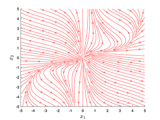
(a) The original f(x)𝑓𝑥f(x)
Refer to caption
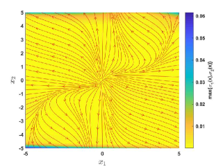
(b) GP approximation of f(x)𝑓𝑥f(x)
Figure 1: The GP approximation for considered example. the color-map shows maximum of standard deviations.
f(x)=[f1(x)f2(x)]=[x1+(cos(x1)1)x2s(x1)+x2],g(x)=[1001],formulae-sequence𝑓𝑥matrixsubscript𝑓1𝑥subscript𝑓2𝑥matrixsubscript𝑥1subscript𝑥11subscript𝑥2𝑠subscript𝑥1subscript𝑥2𝑔𝑥matrix1001\displaystyle f(x)=\begin{bmatrix}f_{1}(x)\\ f_{2}(x)\end{bmatrix}=\begin{bmatrix}x_{1}+(\cos(x_{1})-1)x_{2}\\ -s(x_{1})+x_{2}\end{bmatrix},g(x)=\begin{bmatrix}1&0\\ 0&1\end{bmatrix},

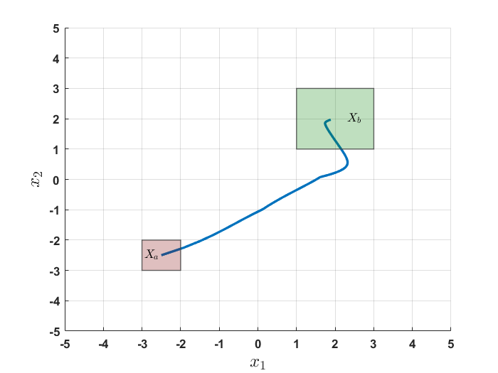
where s(x1)=11+exp(2x1)0.5𝑠subscript𝑥111𝑒𝑥𝑝2subscript𝑥10.5s(x_{1})=\frac{1}{1+exp(-2x_{1})}-0.5 is the shifted sigmoid function. We consider a compact state-space X=[5,5]×[5,5]𝑋5555X=[-5,5]\times[-5,5], initial state-set Xa=[2,3]×[2,3]subscript𝑋𝑎2323X_{a}=[-2,-3]\times[-2,-3], and the goal set Xb=[1,3]×[1,3].subscript𝑋𝑏1313X_{b}=[1,3]\times[1,3]. The functions f1()subscript𝑓1f_{1}(\cdot) and f2()subscript𝑓2f_{2}(\cdot) are continuous, has therefore a finite RKHS norm under the squared exponential kernel on a compact set and complies to Assumption II.1.

For solving Problem II.3, we first approximated the unknown dynamics using GPs with 505050 collected measurments of x𝑥x and corresponding y𝑦y’s, y=f(x)+w𝑦𝑓𝑥𝑤y=f(x)+w, where w𝒩(0,σf2𝑰2)similar-to𝑤𝒩0superscriptsubscript𝜎𝑓2subscript𝑰2w\sim\mathcal{N}(0,\sigma_{f}^{2}\bm{I}_{2}), σf=0.01subscript𝜎𝑓0.01\sigma_{f}=0.01, by running the simulated system with different start states. We used exponential quadratic kernel [20] defined as ki(x,x)=σki2exp(j=12(xixj)22lij2),i{1,2}formulae-sequencesubscript𝑘𝑖𝑥superscript𝑥superscriptsubscript𝜎subscript𝑘𝑖2superscriptsubscript𝑗12superscriptsubscript𝑥𝑖superscriptsubscript𝑥𝑗22superscriptsubscript𝑙𝑖𝑗2𝑖12k_{i}(x,x^{\prime})=\sigma_{k_{i}}^{2}\exp\Big{(}\sum_{j=1}^{2}\frac{(x_{i}-x_{j}^{\prime})^{2}}{-2l_{ij}^{2}}\Big{)},i\in\{1,2\}, where σk1=316subscript𝜎subscript𝑘1316\sigma_{k_{1}}=316 and σk2=25.3subscript𝜎subscript𝑘225.3\sigma_{k_{2}}=25.3 are signal variances and l11=2.9subscript𝑙112.9l_{11}=2.9, l12=177subscript𝑙12177l_{12}=177, l21=1.67subscript𝑙211.67l_{21}=1.67, and l22=50.5subscript𝑙2250.5l_{22}=50.5 are length scales. We use Limited Memory Broyden–Fletcher–Goldfarb–Shanno (L-BFGS-B) algorithm [23, 24] to obtain these parameters. The inferred mean and variance are as in (4) and (5) with σ¯max=max{σ¯1,σ¯2}=0.0616,σ¯1=0.022,σ¯2=0.0616.formulae-sequencesubscript¯𝜎subscript¯𝜎1subscript¯𝜎20.0616formulae-sequencesubscript¯𝜎10.022subscript¯𝜎20.0616\overline{\sigma}_{\max}=\max\{\overline{\sigma}_{1},\overline{\sigma}_{2}\}=0.0616,\overline{\sigma}_{1}=0.022,\overline{\sigma}_{2}=0.0616. Figure 1 depicts the original and the approximated map f(x)𝑓𝑥f(x).

Computing fikisubscriptnormsubscript𝑓𝑖subscript𝑘𝑖\|f_{i}\|_{k_{i}} and γjsubscript𝛾𝑗\gamma_{j}, i{1,2}𝑖12i\in\{1,2\}, is intractable in general. Thus, we used Monte-Carlo method to get the probability bound for the confidence interval given in Proposition III.1.

For a fixed value of βiσ¯i=subscript𝛽𝑖subscript¯𝜎𝑖absent\beta_{i}\overline{\sigma}_{i}= 0.040.040.04, i=1,2𝑖12i=1,2, we get a probability interval for the probability in (6) as {{μ(x)βσ(x)f(x)μ(x)+βσ(x)},xX}[0.9894,0.9907]𝜇𝑥𝛽𝜎𝑥𝑓𝑥𝜇𝑥𝛽𝜎𝑥for-all𝑥𝑋0.98940.9907\mathbb{P}\Big{\{}\{\mu(x)-\beta\sigma(x)\leq f(x)\leq\mu(x)+\beta\sigma(x)\},\forall x\in X\Big{\}}\in[0.9894,0.9907] with confidence 110101superscript10101-10^{-10} using 106superscript10610^{6} realizations. Thus, one can choose the lower bound (1ϵ)2superscript1italic-ϵ2(1-\epsilon)^{2} as 0.98940.98940.9894.

We also computed the value of β~1=7.0878subscript~𝛽17.0878\tilde{\beta}_{1}=7.0878 and β~2=7.0710subscript~𝛽27.0710\tilde{\beta}_{2}=7.0710 as shown in Lemma III.4. To compare the conservativeness of the bounds, we compare the value of β~iσ¯isubscript~𝛽𝑖subscript¯𝜎𝑖\tilde{\beta}_{i}\overline{\sigma}_{i} with Monte-Carlo approach to obtain probability of 1 with confidence of 110101superscript10101-10^{-10}. Using Monte-Carlo approach, the obtained values are β~1σ¯1=0.016subscript~𝛽1subscript¯𝜎10.016\tilde{\beta}_{1}\overline{\sigma}_{1}=0.016 and β~2σ¯2=0.0442subscript~𝛽2subscript¯𝜎20.0442\tilde{\beta}_{2}\overline{\sigma}_{2}=0.0442 and the values obtained using results of Lemma III.4 are β~1σ¯1=0.1559subscript~𝛽1subscript¯𝜎10.1559\tilde{\beta}_{1}\overline{\sigma}_{1}=0.1559 and β~2σ¯2=0.4366subscript~𝛽2subscript¯𝜎20.4366\tilde{\beta}_{2}\overline{\sigma}_{2}=0.4366, respectively. One can readily see the conservatism in the bounds obtained using results of Lemma III.4.
Refer to caption
Figure 2: Simulation of the proposed funnel-based controller using the learned GPs, Xasubscript𝑋𝑎X_{a} and Xbsubscript𝑋𝑏X_{b} are initial and goal sets, respectively. blue line indicates the state trajectory.

With the help of learned mean and variance, we simulate the results using the proposed control law (IV.1). The parameters of the controllers and construction of corresponding funnel functions are as per the Theorem IV.1.
Refer to caption
Refer to caption
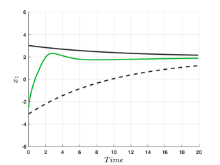
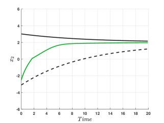
Figure 3: Illustration of trajectories x1subscript𝑥1x_{1} and x2subscript𝑥2x_{2}. The green solid lines represent trajectories, black solid and dashed lines represent upper and lower bounds of funnels, respectively.

The trajectory of the system reaching Xbsubscript𝑋𝑏X_{b} from Xasubscript𝑋𝑎X_{a} is shown in Figure 2. One can readily see from Figure 3, the trajectories x1subscript𝑥1x_{1} and x2subscript𝑥2x_{2} satisfy the constructed funnel bounds.

VI CONCLUSION AND FUTURE WORK

The work proposed a scheme for designing closed-form controller for unknown nonlinear control systems enforcing reachability specifications. We provide a control policy using a funnel-based approach by approximating unknown system dynamics using Gaussian processes. We verified the proposed method using a numerical example. Future research includes incorporating constraints on the input space and extending the results to more complex specifications like linear/signal temporal logic specifications.

References

  • [1] J. Kocijan, Modelling and control of dynamic systems using Gaussian process models.   Springer, 2016.
  • [2] L. Hewing, J. Kabzan, and M. N. Zeilinger, “Cautious model predictive control using Gaussian process regression,” IEEE Transactions on Control Systems Technology, 2019.
  • [3] G. Chowdhary, H. A. Kingravi, J. P. How, and P. A. Vela, “Bayesian nonparametric adaptive control using Gaussian processes,” transactions on neural networks and learning systems, vol. 26, no. 3, pp. 537–550, 2014.
  • [4] T. Beckers, D. Kulić, and S. Hirche, “Stable gaussian process based tracking control of euler–lagrange systems,” Automatica, vol. 103, pp. 390–397, 2019.
  • [5] A. Capone and S. Hirche, “Backstepping for partially unknown nonlinear systems using gaussian processes,” Control Systems Letters, vol. 3, no. 2, pp. 416–421, 2019.
  • [6] J. Umlauft, T. Beckers, M. Kimmel, and S. Hirche, “Feedback linearization using Gaussian processes,” in 56th Annual Conference on Decision and Control (CDC).   IEEE, 2017, pp. 5249–5255.
  • [7] F. Berkenkamp, A. P. Schoellig, and A. Krause, “Safe controller optimization for quadrotors with Gaussian processes,” in International Conference on Robotics and Automation (ICRA).   IEEE, 2016, pp. 491–496.
  • [8] A. K. Akametalu, J. F. Fisac, J. H. Gillula, S. Kaynama, M. N. Zeilinger, and C. J. Tomlin, “Reachability-based safe learning with Gaussian processes,” in 53rd Conference on Decision and Control.   IEEE, 2014, pp. 1424–1431.
  • [9] P. Jagtap, G. J. Pappas, and M. Zamani, “Control barrier functions for unknown nonlinear systems using Gaussian processes,” in 59th Conference on Decision and Control (CDC).   IEEE, 2020, pp. 3699–3704.
  • [10] H. Ravanbakhsh, S. Sankaranarayanan, and S. A. Seshia, “Formal policy learning from demonstrations for reachability properties,” in International Conference on Robotics and Automation (ICRA).   IEEE, 2019, pp. 6037–6043.
  • [11] M. Rungger and M. Zamani, “SCOTS: A tool for the synthesis of symbolic controllers,” in Proceedings of the 19th international conference on hybrid systems: Computation and control, 2016, pp. 99–104.
  • [12] J. Lygeros, C. Tomlin, and S. Sastry, “Controllers for reachability specifications for hybrid systems,” Automatica, vol. 35, no. 3, pp. 349–370, 1999.
  • [13] S. Junges, N. Jansen, and S. A. Seshia, “Enforcing almost-sure reachability in pomdps,” in International Conference on Computer Aided Verification.   Springer, 2021, pp. 602–625.
  • [14] R. Vignali and M. Prandini, “A method for detecting relevant inputs while satisfying a reachability specification for piecewise affine systems,” in Conference on Control Applications (CCA).   IEEE, 2016, pp. 538–543.
  • [15] C. P. Bechlioulis and G. A. Rovithakis, “A low-complexity global approximation-free control scheme with prescribed performance for unknown pure feedback systems,” Automatica, vol. 50, no. 4, pp. 1217–1226, 2014.
  • [16] X. Bu, “Prescribed performance control approaches, applications and challenges: A comprehensive survey,” Asian Journal of Control, 2021.
  • [17] M. W. Seeger, S. M. Kakade, and D. P. Foster, “Information consistency of nonparametric Gaussian process methods,” Transactions on Information Theory, vol. 54, no. 5, pp. 2376–2382, 2008.
  • [18] V. I. Paulsen and M. Raghupathi, An introduction to the theory of reproducing kernel Hilbert spaces.   Cambridge University Press, 2016, vol. 152.
  • [19] J. Umlauft, L. Pöhler, and S. Hirche, “An uncertainty-based control Lyapunov approach for control-affine systems modeled by Gaussian process,” IEEE Control Systems Letters, vol. 2, no. 3, pp. 483–488, 2018.
  • [20] C. K. Williams and C. E. Rasmussen, Gaussian processes for machine learning.   MIT press Cambridge, MA, 2006, vol. 2, no. 3.
  • [21] N. Srinivas, A. Krause, S. M. Kakade, and M. W. Seeger, “Information-theoretic regret bounds for Gaussian process optimization in the bandit setting,” Transactions on Information Theory, vol. 58, no. 5, pp. 3250–3265, 2012.
  • [22] K. Hashimoto, A. Saoud, M. Kishida, T. Ushio, and D. Dimarogonas, “Learning-based symbolic abstractions for nonlinear control systems,” in arXiv preprint arXiv:2004.01879, 2021.
  • [23] R. H. Byrd, P. Lu, J. Nocedal, and C. Zhu, “A limited memory algorithm for bound constrained optimization,” SIAM Journal on Scientific Computing, vol. 16, no. 5, pp. 1190–1208, 1995. [Online]. Available: https://doi.org/10.1137/0916069
  • [24] C. Zhu, R. H. Byrd, P. Lu, and J. Nocedal, “Algorithm 778: L-BFGS-B: fortran subroutines for large-scale bound-constrained optimization,” ACM Trans. Math. Softw., vol. 23, no. 4, p. 550–560, dec 1997.