On $\mathcal{N}{=}4$ supersymmetry enhancements
in three dimensions

Benjamin Assel¹, Yuji Tachikawa² and Alessandro Tomasiello³

1	Paris, France. benjamin.assel@gmail.com
2	Kavli Institute for the Physics and Mathematics of the Universe (WPI),
	University of Tokyo, Kashiwa, Chiba 277-8583, Japan
	yuji.tachikawa@ipmu.jp
3	Dipartimento di Matematica, Università di Milano-Bicocca, and
	INFN, sezione di Milano-Bicocca, I-20126 Milano, Italy
	alessandro.tomasiello@unimib.it

We introduce a class of 3d theories consisting of strongly-coupled $\mathcal{N}{=}4$ systems coupled to $\mathcal{N}{=}3$ Chern–Simons gauge multiplets, which exhibit $\mathcal{N}{=}4$ enhancements when a peculiar condition on the Chern–Simons levels is met. An example is the $SU(N)^{3}$ Chern–Simons theory coupled to the 3d $T_{N}$ theory, which enhances to $\mathcal{N}{=}4$ when $1/k_{1}+1/k_{2}+1/k_{3}=0$. We also show that some but not all of these $\mathcal{N}{=}4$ enhancements can be understood by considering M5-branes on a special class of Seifert manifolds. Our construction provides a large class of $\mathcal{N}{=}4$ theories which have not been studied previously.

1 Introduction and summary

The aim of this paper is to discuss a class of three-dimensional $\mathcal{N}{=}4$ supersymmetric theories which have rarely been studied in the literature. There are two complementary motivations leading to the same class of theories, as we will see below.

Our first motivation is in the context of highly-supersymmetric Chern–Simons-matter theories. As is well-known, the highest supersymmetry one can achieve in generic Chern–Simons-matter systems is $\mathcal{N}{=}3$ [Sch04, GY07]. It is also known that, when the matter content and the gauge group are carefully chosen, the supersymmetry can show further enhancements to $\mathcal{N}{=}4$ [GW08a, HLL⁺08a], $\mathcal{N}{=}5$ [HLL⁺08b], $\mathcal{N}{=}6$ [ABJM08, ABJ08], and $\mathcal{N}{=}8$ [Gus07, BL07]. Almost all of these theories use only bifundamental matter fields, except a single case mentioned implicitly in [GW08a], which is an $SU(2)^{3}$ Chern–Simons (CS) theory coupled to a half-hypermultiplet in the trifundamental representation.

This theory is generically $\mathcal{N}{=}3$ supersymmetric, but shows $\mathcal{N}{=}4$ enhancement if and only if the three levels $k_{1,2,3}$ satisfy the relation $1/k_{1}+1/k_{2}+1/k_{3}=0$. What we do here is to generalize this example using another idea already mentioned in [GW08a], of using strongly-coupled $\mathcal{N}{=}4$ systems with curved Higgs branches as the matter content. For example, we will show that the theory composed of $SU(N)^{3}$ Chern–Simons vector multiplets coupled to the 3d $T_{N}$ theory enjoys $\mathcal{N}{=}4$ enhancement in the same manner, if and only if $1/k_{1}+1/k_{2}+1/k_{3}=0$. We will further generalize it to a class-S-like construction.

Our second motivation is in the study of supersymmetric compactifications of M5-branes on 3-manifolds. Their general study was initiated in [TY11] for mapping tori and [DGG11a] for triangulated manifolds. In these cases, the 3-manifolds are hyperbolic, and the resulting theories generically have $\mathcal{N}{=}2$ supersymmetry. A far simpler class of theories was studied slightly before them in [BTX10], where the compactifications on $S^{1}$ times surfaces were considered. They can be studied as the $S^{1}$ compactification of 4d class S theories, and have $\mathcal{N}{=}4$ supersymmetry.

In the general classification of 3-manifolds conjectured by Thurston and proved recently, there are manifolds which lie between these two extremes, known as Seifert manifolds and graph manifolds. Such compactifications have not been studied as thoroughly as the hyperbolic ones, but the 3d theories which result from them have already been worked out in e.g. [GGP13, PY15, GPV16, GPPV17, EKSNW19, CGK20], although determining them was usually not the main objective of these papers. Generically they have $\mathcal{N}{=}2$ supersymmetry. In this paper, we find several spaces which lead to $\mathcal{N}{=}4$ supersymmetry. A simple subclass consists of Seifert fibrations over a sphere with three singular fibers, whose Seifert parameters $q_{i}/p_{i}$ for $i=1,2,3$ sum to zero, $\sum_{i}q_{i}/p_{i}=0$. When $q_{1,2,3}=1$, the resulting 3d theories turn out to be equivalent to the theories we mentioned above, coming from our first motivation.

In this particular subclass, the supersymmetry enhancement we observe is the same both in the field theoretical analysis and in the analysis using the geometry of 3-manifolds. This, however, is not always the case, and there are a large number of examples where the supersymmetry seen field theoretically is higher than what can be gleaned from the geometry, as we will describe in more detail in the rest of the paper. The authors would hope to come back to this issue in the future.

The rest of the paper is organized as follows. In Sec. 2, we start by recalling the supersymmetry enhancement mechanism in 3d Chern–Simons-matter systems. We then discuss the enhancement of the supersymmetry from $\mathcal{N}{=}3$ to $\mathcal{N}{=}4$ of $SU(2)^{3}$ Chern–Simons theory coupled to a half-hypermultiplet in the trifundamental representation, and study how it can be generalized to the case of $SU(N)^{3}$ Chern–Simons theory coupled to the $T_{N}$ theory.

After making some further generalization, we move on to Sec. 3, where we consider M5-branes compactified on 3-manifolds. After very briefly reviewing the classification of 3-manifolds, we study M5-branes on Seifert manifolds and on graph manifolds. We will see that the resulting 3d theories realize the 3d Chern–Simons-matter systems we discuss in Sec. 2. We will also see that the reduction of the holonomy of 3-manifolds used in the construction does explain the $\mathcal{N}{=}4$ enhancement in some cases, but not all.

In Appendix A and in Appendix B, we study the homology groups and the possible supergravity backgrounds on the 3-manifolds used in Sec. 3, in order to find any indication of supersymmetry enhancement when the holonomy reduction does not happen. Unfortunately, we do not find any definitive results, although we do find some hints.

In the final Appendix C, we make some further comments on the property of the 3d $SL(2,\mathbb{Z})$ duality wall theory, and of the theory obtained by diagonally gauging its $SU(N)$ flavor symmetry. This is done using the results obtained in the course of Sec. 3 and the computation of the contact terms using localization, following [CDF⁺12a, CDF⁺12b].

Before proceeding, we pause here to mention that we will be cavalier about the choice of the global structure of the gauge group and also about the possible presence of almost decoupled topological sectors. In particular, we will stick to the careless habit of not distinguishing Lie algebras and Lie groups in the notations, which was prevalent in our community until several years ago. It would surely be interesting to study these issues carefully, which was in fact one of the main motivations in the previous study [EKSNW19] on 3d theories coming from Seifert manifolds, although not in the context of supersymmetry enhancements.

We also note that there recently appeared a paper [CGK22] where, among others, $\mathcal{N}{=}4$ enhancements of 6d $\mathcal{N}{=}(2,0)$ theories on non-hyperbolic 3-manifolds $M$ were discussed. The results here and there cannot be readily compared, because their derivation is rather different, and also because they considered 3d theories $T_{\text{irred}}[M]$ associated to irreducible $SL(2)$ connections on $M$, while we consider $T_{\text{full}}[M]$ which is the ordinary compactification on $M$; see [CDGS14, GY18a] for the difference. That said, it would be interesting to study the interconnection between the two approaches, as the 3-manifolds discussed in the two papers do overlap.

2 Highly-supersymmetric Chern–Simons-matter theories

In this section, we introduce the readers to our first class of 3d Chern–Simons-matter theories which show enhancements to $\mathcal{N}{=}4$ supersymmetry. This is done from the study of highly-supersymmetric Chern–Simons-matter theories.

When the matter content is generic, supersymmetric Chern–Simons-matter theories are only possible up to $\mathcal{N}{=}3$ supersymmetry. Theories with higher supersymmetry were first constructed in [Gus07, BL07] in the $\mathcal{N}{=}8$ cases using 3-algebras. The construction was motivated by the then-popular beliefs that something other than ordinary Lie algebras would be necessary.

It was soon realized, however, that they can be written in terms of ordinary Lie algebras [BLS08], and generalizations to $\mathcal{N}{=}4$ theories were performed using the 3d $\mathcal{N}{=}1$ superfield formalism in [GW08a, HLL⁺08a]. Slightly later, the famous $\mathcal{N}{=}6$ theory of Aharony, Bergman, Jafferis and Maldacena was found in [ABJM08] using the 3d $\mathcal{N}{=}2$ superfield formalism. In fact, all the supersymmetry enhancements listed here can be understood by adapting this 3d $\mathcal{N}{=}2$ superfield method [ST08]. Here we provide a quick review of the mechanism of the enhancement, and then introduce our first class of theories showing $\mathcal{N}{=}4$ enhancements which were not studied previously.

2.1 Mechanism of the enhancement

Enhancement from $\mathcal{N}{=}2$ to $\mathcal{N}{=}4$ in 4d:

Let us start by recalling a method to understand the structure of 4d $\mathcal{N}{=}4$ super Yang–Mills theories. It is well-known that we can write down a 4d $\mathcal{N}{=}2$ gauge theory for any gauge group and hypermultiplets. Let us pick a gauge group $G$ and let the hypermultiplet be in its adjoint representation. In the $\mathcal{N}{=}1$ language, the superpotential has the form

$$W\propto\mathop{\mathrm{tr}}\Phi[A,B]$$ (2.1)

where $\Phi$ is the scalar in the vector multiplet and $(A,B)$ form the hypermultiplet. In the $\mathcal{N}{=}1$ perspective, it is clear that the theory is symmetric under the $SU(3)_{F}$ flavor symmetry acting on three adjoint scalars $\Phi$, $A$ and $B$, from the structure of the superpotential. Meanwhile, in the $\mathcal{N}{=}2$ perspective, the $SU(2)_{R}$ symmetry acts on $(A,B^{\dagger})$. Therefore, $SU(2)_{R}$ and $SU(3)_{F}$ do not commute, and necessarily combine to a larger R-symmetry, signaling the enhancement of the supersymmetry to $\mathcal{N}{=}4$.

Enhancement from $\mathcal{N}{=}3$ to $\mathcal{N}{=}N$ in 3d:

In three dimensions, we can similarly achieve $\mathcal{N}{=}3$ supersymmetry with general gauge group $G=\prod_{i}G_{i}$ with non-zero Chern–Simons terms, and an arbitrary representation $R$ for the hypermultiplets. The superpotential in $\mathcal{N}{=}2$ language is

$$W\propto\sum_{i}\left(\mathop{\mathrm{tr}}\Phi_{i}\mu_{i}-\frac{k_{i}}{2}\mathop{\mathrm{tr}}\Phi_{i}^{2}\right),$$ (2.2)

where $\Phi_{i}$ is the adjoint scalar in the $i$-th Chern–Simons supermultiplet of level $k_{i}$ and $\mu_{i}$ is the moment map operator constructed from the hypermultiplets.

We note that this system preserves $\mathcal{N}{=}4$ supersymmetry when $k_{i}=0$. In this case, the superpotential possesses a manifest $U(1)$ symmetry assigning charge $+2$ and $-2$ to $\mu_{i}$ and $\Phi_{i}$. This is in fact a part of $SO(4)_{R}$ symmetry of the $\mathcal{N}{=}4$ supersymmetry algebra, and is broken by the term proportional to $k_{i}$ in (2.2) when it is nonzero.

For the moment, let us assume $k_{i}\neq 0$. As the adjoint scalars $\Phi_{i}$ have no kinetic term, they can be integrated out, giving

$$W\propto\sum_{i}\frac{1}{k_{i}}\mathop{\mathrm{tr}}\mu_{i}^{2}.$$ (2.3)

When the matter representations and the levels are chosen carefully, this $W$ can have a flavor symmetry not commuting with the $\mathcal{N}{=}3$ R-symmetry, signaling the enhancement to supersymmetry higher than $\mathcal{N}{=}3$.

In three dimensions, an $\mathcal{N}{=}N$ superconformal theory has $SO(N)_{R}$ flavor symmetry. The $\mathcal{N}{=}2$ formalism makes only $SO(2)_{R}$ symmetry manifest, and therefore we should see an additional $SO(N-2)$ flavor symmetry in the $\mathcal{N}{=}2$ superpotential (2.3) to have the enhancement.

$\mathcal{N}{=}6$ theories of ABJ(M):

As an example, consider the $\mathcal{N}{=}3$ $U(N)_{k}\times U(N^{\prime})_{-k^{\prime}}$ Chern–Simons theory with two bifundamentals $A_{i}$, $B^{i}$ where $i=1,2$. The superpotential (2.3)

$$W\propto\frac{1}{k}\mathop{\mathrm{tr}}(A_{i}B^{i})^{2}-\frac{1}{k^{\prime}}\mathop{\mathrm{tr}}(B^{i}A_{i})^{2}$$ (2.4)

simplifies, if $k=k^{\prime}$, to

$$\propto\frac{1}{k}\mathop{\mathrm{tr}}A_{i}B^{a}A_{j}B^{b}\epsilon^{ij}\epsilon_{ab}$$ (2.5)

showing the flavor symmetry $SU(2)\times SU(2)=SO(6-2)$. This flavor symmetry does not commute with $SO(3)_{R}$, under which $A_{i}$ forms a doublet with $(B^{i})^{\dagger}$. This means that the theory enhances to $\mathcal{N}{=}6$ when $k=k^{\prime}$; this is the famous theory of Aharony-Maldacena-Bergman-Jafferis or Aharony-Bergman-Jafferis, depending on $N=N^{\prime}$ or $N\neq N^{\prime}$ [ABJM08, ABJ08].

$\mathcal{N}{=}4$ theories of Gaiotto–Witten:

As another class of examples, consider the $\mathcal{N}{=}3$ theory with a general gauge group $G=\prod_{i}G_{i}$ and (half-)hypermultiplets in a general representation $R$. Let us suppose that the superpotential (2.3) simply vanishes,

$$W\propto\sum_{i}\frac{1}{k_{i}}\mathop{\mathrm{tr}}\mu_{i}^{2}=0,$$ (2.6)

thanks to a careful choice of $G$ and $R$.

Let us see that this means that the theory enhances to $\mathcal{N}{=}4$ supersymmetry. Before coupling to $\mathcal{N}{=}3$ Chern–Simons multiplets, the theory of free (half-)hypermultiplets has $\mathcal{N}{=}4$ supersymmetry, with four supercharges $Q_{1,2,3,4}$, with R-symmetries $J_{ij}$ mapping $Q_{i}$ to $Q_{j}$.

Let us say that we are using an $\mathcal{N}{=}2$ subalgebra including $Q_{1,2}$ and $J_{12}$ for our $\mathcal{N}{=}2$ description. When the superpotential vanishes as in (2.6), we have a $U(1)=SO(4-2)$ flavor symmetry, assigning the charge $+1$ for all $\mathcal{N}{=}2$ chiral multiplets. This $U(1)$ symmetry is $J_{34}$ of the original theory of hypermultiplets.

Now, the $\mathcal{N}{=}3$ Chern–Simons multiplets are known to preserve $Q_{1,2,3}$. We now found that $J_{34}$ is preserved. Therefore, $Q_{4}$ is also preserved, meaning that the gauged theory has $\mathcal{N}{=}4$ supersymmetry. The condition was originally obtained by Gaiotto and Witten in [GW08a], using the $\mathcal{N}{=}1$ superfield formalism.

The construction can be generalized by replacing (half-)hypermultiplets by a more general strongly-coupled 3d $\mathcal{N}{=}4$ theory $T$ with $G$ symmetry with $SO(4)_{R}$ symmetry. We note that such a theory $T$, regarded as an $\mathcal{N}{=}2$ theory, has a $U(1)$ flavor symmetry $J_{34}$ assigning charge $+2$ to the moment map operators $\mu$. When we gauge the $G$ symmetry with $\mathcal{N}{=}3$ Chern–Simons couplings, the $\mathcal{N}{=}2$ superpotential (2.3) breaks this $U(1)$ flavor symmetry for generic levels. However, when the relation (2.6) is satisfied, this $U(1)=SO(4-2)$ flavor symmetry is restored, and the gauged theory enhances to $\mathcal{N}{=}4$. This strongly-coupled generalization was already mentioned in [GW08a], although in the $\mathcal{N}{=}1$ superfield language.

It was also found in the original article [GW08a] that the condition (2.6) when the matter content is given by (half-)hypermultiplets is equivalent to the statement that $\mathfrak{g}\oplus R$ forms a super Lie algebra with an invariant non-degenerate trace. In more detail, 1) $\mathfrak{g}$ and $R$ are the bosonic and the fermionic part of the super Lie algebra, respectively, 2) the vanishing (2.6) is equivalent to the fermion-fermion-fermion part of the super Jacobi identity, and 3) the ratio of the levels $\{k_{i}\}$ is a part of the structure constants. As the classification of super Lie algebras with invariant traces is long known [Kac77], this gives us all theories where Chern–Simons gauge fields couple to (half-)hypermultiplets such that the supersymmetry enhances to $\mathcal{N}{=}4$ from the condition (2.6).

An example of this type of theories is to take the super Lie algebra to be $OSp(2m|2n)$, which corresponds to the gauge theory $O(2m)_{2k}\times USp(2n)_{-k}$ with a half-hypermultiplet in the bifundamental representation. This turns out to be the starting point of our generalization.

2.2 New $\mathcal{N}{=}4$ theories

2.2.1 Gauged $T_{N}$ theory

Let us now consider the special case of $OSp(4|2)$. The corresponding gauge theory has the gauge group $SO(4)\times USp(2)\simeq SU(2)_{1}\times SU(2)_{2}\times SU(2)_{3}$, with a half-hypermultiplet in $\mathbf{4}\otimes\mathbf{2}\simeq\mathbf{2}_{1}\otimes\mathbf{2}_{2}\otimes\mathbf{2}_{3}$, which we denote by $Q_{aiu}$. The condition for the $\mathcal{N}{=}4$ enhancement (2.6) is

$$W\propto\frac{1}{k_{1}}\mathop{\mathrm{tr}}(\mu_{1})^{2}+\frac{1}{k_{2}}\mathop{\mathrm{tr}}(\mu_{2})^{2}+\frac{1}{k_{3}}\mathop{\mathrm{tr}}(\mu_{3})^{2}=0$$ (2.7)

where $k_{1,2,3}$ and $\mu_{1,2,3}$ are the levels and the moment map operators for $SU(2)_{1,2,3}$. More explicitly, $\mu_{1,2,3}$ are given by

$$\mu_{1}{}^{{c}}{}_{{b}}=\epsilon^{{ca}}\mu_{1,{ab}},\quad\mu_{2}{}^{{k}}{}_{{j}}=\epsilon^{{ki}}\mu_{2,{ij}},\quad\mu_{3}{}^{{w}}{}_{{v}}=\epsilon^{{wu}}\mu_{3,{uv}}$$ (2.8)

where

$$\mu_{1,{ab}}=\epsilon^{{ij}}\epsilon^{{uv}}Q_{{a}{i}{u}}Q_{{b}{j}{v}},\quad\mu_{2,{ij}}=\epsilon^{{ab}}\epsilon^{{uv}}Q_{{a}{i}{u}}Q_{{b}{j}{v}},\quad\mu_{3,{uv}}=\epsilon^{{ab}}\epsilon^{{ij}}Q_{{a}{i}{u}}Q_{{b}{j}{v}}$$ (2.9)

which satisfy the crucial relation

$$\mathop{\mathrm{tr}}(\mu_{1})^{2}=\mathop{\mathrm{tr}}(\mu_{2})^{2}=\mathop{\mathrm{tr}}(\mu_{3})^{2}.$$ (2.10)

Therefore, the enhancement condition (2.7) is satisfied if and only if we have

$$\frac{1}{k_{1}}+\frac{1}{k_{2}}+\frac{1}{k_{3}}=0.$$ (2.11)

Physically, we need to require that the levels are integers. Luckily for us, the relation (2.11) has many integer solutions, e.g. $(k_{1},k_{2},k_{3})=(pq,qr,rp)$ with $p+q+r=0$ and $p,q,r\in\mathbb{Z}_{\neq 0}$.

As mentioned above, the ratio of the levels solving (2.7) translates to the structure constants of the super Lie algebra. The relation (2.11) means that $OSp(4|2)$ has a one-parameter family of structure constants. In fact, among the classification in [Kac77] of super Lie algebras, $D(2,1)=OSp(4|2)$ is the only case where the structure constants come in a family, and is often denoted as $D(2,1;\alpha)$ to make this fact explicit.

Let us now generalize this example, by replacing $SU(2)^{3}$ and $Q_{aiu}$ by $SU(N)^{3}$ and the 3d $T_{N}$ theory. Here the 3d $T_{N}$ theory is a strongly-coupled 3d $\mathcal{N}{=}4$ SCFT having $SU(N)^{3}$ symmetry, obtained by compactifying the 4d $T_{N}$ theory on $S^{1}$. Equivalently, it is given by wrapping $N$ M5-branes on $S^{1}$ times a sphere with three full punctures. Its chiral ring is summarized e.g. in [Tac15]. Crucially, the three $SU(N)$ moment map operators $\mu_{1,2,3}$ satisfy the relations (2.10), as we will see in Sec. 3.2.3; therefore the combined system has enhanced $\mathcal{N}{=}4$ supersymmetry if the relation (2.11) is satisfied. The structure of the theory can be depicted as in Fig. 1.

Figure 1: $T_{N}$ theory gauged with $SU(N)_{k_{1}}\times SU(N)_{k_{2}}\times SU(N)_{k_{3}}$. The supersymmetry enhances to $\mathcal{N}{=}4$ when $1/k_{1}+1/k_{2}+1/k_{3}=0$.

There is an easy generalization of this construction if one knows the basics of 3d class S theories, first studied in [BTX10]. Let us take two copies of the 3d $T_{N}$ theory, and gauge a diagonal subgroup of two $SU(N)$ flavor symmetries, each belonging to a separate $T_{N}$ theory, by an $\mathcal{N}{=}4$ $SU(N)$ vector multiplet. This is the compactification of 6d $\mathcal{N}{=}(2,0)$ theory on $S^{1}$ times a sphere with four punctures. The resulting theory has $SU(N)^{4}$ flavor symmetry, whose moment map fields satisfy

$$\mathop{\mathrm{tr}}(\mu_{1})^{2}=\mathop{\mathrm{tr}}(\mu_{2})^{2}=\mathop{\mathrm{tr}}(\mu_{3})^{2}=\mathop{\mathrm{tr}}(\mu_{4})^{2}.$$ (2.12)

More generally, we can take $n-1$ copies of the $T_{N}$ theory and couple $\mathcal{N}{=}4$ $SU(N)$ vector multiplets appropriately, and realize the compactification of 6d $\mathcal{N}{=}(2,0)$ theory on $S^{1}$ times a sphere with $n$ punctures. Let us denote the resulting theory by $T_{N,n}$. It has $SU(N)^{n}$ symmetry, whose moment map fields satisfy the basic relation that

$$\mathop{\mathrm{tr}}(\mu_{i})^{2}\quad\text{is independent of $i=1,2,\ldots,n$.}$$ (2.13)

The derivation of this important relation is reviewed in Sec. 3.2.3.

We can then couple the $SU(N)^{n}$ flavor symmetry to $\mathcal{N}{=}3$ $SU(N)$ Chern–Simons gauge fields with levels $k_{i}$ for $i=1,\ldots,n$. Exactly as before, we find that the superpotential after the elimination of adjoint scalars vanishes when

$$\sum_{i}\frac{1}{k_{i}}=0,$$ (2.14)

leading to $\mathcal{N}{=}4$ enhancements.

So far these theories might look like a mere curiosity. In the next section we are going to find a geometric interpretation for this enhancement. Before getting there, let us consider a generalization of this construction.

2.2.2 Further generalizations

Figure 2: Two $T_{N}$ theories gauged with $SU(N)_{k_{1}}\times SU(N)_{k_{2}}\times SU(N)_{k_{3}}$.

Let us now consider the theory depicted in Fig. 2. Namely, we take two copies of 3d $T_{N}$ theory. For each $SU(N)$ symmetry of one $T_{N}$ theory, we pick an $SU(N)$ symmetry from the other $T_{N}$ theory, and couple their diagonal combination to an $\mathcal{N}{=}3$ $SU(N)$ Chern–Simons multiplet. Denoting the levels by $k_{1,2,3}$, we see that the superpotential in the $\mathcal{N}{=}2$ description is

$$W= -\frac{k_{1}}{2}\mathop{\mathrm{tr}}(\Phi_{1})^{2}+\mathop{\mathrm{tr}}\Phi_{1}(\mu_{1}^{(1)}+\mu_{1}^{(2)})$$ (2.15)

$$-\frac{k_{2}}{2}\mathop{\mathrm{tr}}(\Phi_{2})^{2}+\mathop{\mathrm{tr}}\Phi_{2}(\mu_{2}^{(1)}+\mu_{2}^{(2)})$$

$$-\frac{k_{3}}{2}\mathop{\mathrm{tr}}(\Phi_{3})^{2}+\mathop{\mathrm{tr}}\Phi_{3}(\mu_{3}^{(1)}+\mu_{3}^{(2)})$$

where $\Phi_{i}$ is the adjoint scalar in the $i$-th $\mathcal{N}{=}3$ Chern–Simons multiplet and $\mu_{1,2,3}^{(a)}$ is the moment map field of $SU(N)^{3}$ of the $a$-th $T_{N}$ theory.

Eliminating $\Phi_{1,2,3}$, we find that the superpotential becomes

$$W= \frac{1}{2}\left(\frac{1}{k_{1}}+\frac{1}{k_{2}}+\frac{1}{k_{3}}\right)(\mathop{\mathrm{tr}}(\mu^{(1)})^{2}+\mathop{\mathrm{tr}}(\mu^{(2)})^{2})$$ (2.16)

$$+\frac{1}{k_{1}}\mathop{\mathrm{tr}}\mu_{1}^{(1)}\mu_{1}^{(2)}+\frac{1}{k_{2}}\mathop{\mathrm{tr}}\mu_{2}^{(1)}\mu_{2}^{(2)}+\frac{1}{k_{3}}\mathop{\mathrm{tr}}\mu_{3}^{(1)}\mu_{3}^{(2)}$$

where we used the chiral ring relation $\mathop{\mathrm{tr}}(\mu_{1}^{(1)})^{2}=\mathop{\mathrm{tr}}(\mu_{2}^{(1)})^{2}=\mathop{\mathrm{tr}}(\mu_{3}^{(1)})^{2}=:\mathop{\mathrm{tr}}(\mu^{(1)})^{2}$ for the first $T_{N}$ theory, and similarly for the second copy. The superpotential simplifies when

$$\frac{1}{k_{1}}+\frac{1}{k_{2}}+\frac{1}{k_{3}}=0$$ (2.17)

to

$$W=\frac{1}{k_{1}}\mathop{\mathrm{tr}}\mu_{1}^{(1)}\mu_{1}^{(2)}+\frac{1}{k_{2}}\mathop{\mathrm{tr}}\mu_{2}^{(1)}\mu_{2}^{(2)}+\frac{1}{k_{3}}\mathop{\mathrm{tr}}\mu_{3}^{(1)}\mu_{3}^{(2)},$$ (2.18)

which has a $U(1)=SO(4-2)$ flavor symmetry assigning charge $+2$ to the moment map fields of the first $T_{N}$ theory and charge $-2$ to those of the second $T_{N}$ theory. This signifies that the theory enhances to $\mathcal{N}{=}4$.

To give some more detail, let $Q^{(a)}_{1,2,3,4}$ be four supercharges of the $a$-th $T_{N}$ theory, and $J^{(a)}_{ij}$ be the R-symmetry of the $a$-th theory sending $Q^{(a)}_{i}$ to $Q^{(a)}_{j}$. The $\mathcal{N}{=}3$ Chern–Simons couplings preserve $Q_{i}:=Q^{(1)}_{i}+Q^{(2)}_{i}$ for $i=1,2,3$, and our $\mathcal{N}{=}2$ formalism makes $Q_{1}$, $Q_{2}$ and $J_{12}:=J_{12}^{(1)}+J_{12}^{(2)}$ manifest. The $U(1)$ symmetry preserved by the simplified superpotential (2.18) is $J_{34}^{\prime}:=J_{34}^{(1)}-J_{34}^{(2)}$. Note the relative minus sign, assigning opposite $U(1)$ charges to $\mu_{i}^{(1)}$ and $\mu_{i}^{(2)}$. This $U(1)$ symmetry sends $Q_{3}=Q^{(1)}_{3}+Q^{(2)}_{3}$ to $Q_{4}^{\prime}:=Q^{(1)}_{4}-Q^{(2)}_{4}$. This type of $\mathcal{N}{=}4$ enhancements was first found in [HLL⁺08a] in the Lagrangian case.

Note that the operation $(Q_{1},Q_{2},Q_{3},Q_{4})\mapsto(Q_{1},Q_{2},Q_{3},-Q_{4})$ in an $\mathcal{N}{=}4$ theory is the 3d mirror symmetry which exchanges the Higgs branch and the Coulomb branch and sends hypermultiplets to twisted hypermultiplets. Therefore, when the supersymmetry enhances to $\mathcal{N}{=}4$ in this theory, the assignment of $\mathcal{N}{=}4$ supercharges is different between the first copy and the second copy of the $T_{N}$ theory. The $SU(2)$ R-symmetry acting on the Coulomb branch of one $T_{N}$ theory is mapped to the $SU(2)$ R-symmetry acting on the Higgs branch of the other $T_{N}$ theory. In other words, there is no standard assignment of the Coulomb branch and the Higgs branch to the final $\mathcal{N}{=}4$ theory.

Figure 3: A graph encoding the coupling of $T_{N,n}$ theories and $\mathcal{N}{=}3$ Chern–Simons multiplets. Every link $e$ represents a coupling to a CS level $k_{e}$ as in (2.19).

Let us conclude this section by making a further generalization. We take a bipartite graph, an example of which is shown in Fig. 3. There, each $n$-valent node is a copy of the $T_{N,n}$ theory, obtained by compactifying 6d $\mathcal{N}{=}(2,0)$ theory on $S^{1}$ times $S^{2}$ with $n$ full punctures. Recall that it has $SU(N)^{n}$ symmetry whose moment map fields satisfy (2.13).

Next, each edge $e$ connecting two nodes is an $\mathcal{N}{=}3$ $SU(N)$ Chern–Simons multiplet coupling to the diagonal subgroup of two $SU(N)$ symmetries, one from the $T_{N,n}$ theory on a black node, and another from the $T_{N,n}$ theory on a white node, assigned with a non-zero Chern–Simons level $k_{e}$. The superpotential is given by

$$W=\sum_{e:\text{edge}}\left[-\frac{k_{e}}{2}\mathop{\mathrm{tr}}(\Phi_{e})^{2}+\mathop{\mathrm{tr}}\Phi_{e}(\mu_{e}^{\text{black}}+\mu_{e}^{\text{white}})\right].$$ (2.19)

Integrating out the $\mathcal{N}{=}2$ adjoint scalars, we get

$$W =\sum_{e:\text{edge}}\left[\frac{1}{2k_{e}}\big{(}\mathop{\mathrm{tr}}(\mu_{e}^{\text{black}})^{2}+\mathop{\mathrm{tr}}(\mu_{e}^{\text{white}})^{2}))+\frac{1}{k_{e}}\mathop{\mathrm{tr}}\mu_{e}^{\text{black}}\mu_{e}^{\text{white}}\right]$$ (2.20)

$$=\sum_{e:\text{edge}}\frac{1}{k_{e}}\mathop{\mathrm{tr}}\mu_{e}^{\text{black}}\mu_{e}^{\text{white}}+\sum_{v:\text{node}}\sum_{\begin{subarray}{c}e:\text{edge}\\ \text{connecting to $v$}\end{subarray}}\frac{1}{2k_{e}}\mathop{\mathrm{tr}}(\mu_{v,e})^{2}$$ (2.21)

where $\mu_{v,e}$ is the moment map of the $SU(N)$ flavor symmetry of the $T_{N,n}$ theory at the node $v$ coupled to the Chern–Simons gauge multiplet for the edge $e$. Thanks to the chiral ring relation (2.13), $\mathop{\mathrm{tr}}(\mu_{v,e})^{2}$ is independent of $e$. Therefore, when the sum of the inverse of the three Chern–Simons levels at each node vanishes, i.e. when

$$\sum_{\begin{subarray}{c}e:\text{edge}\\ \text{connecting to $v$}\end{subarray}}\frac{1}{k_{e}}=0\,\quad\text{for each node $v$},$$ (2.22)

the superpotential becomes

$$W=\sum_{e:\text{edge}}\frac{1}{k_{e}}\mathop{\mathrm{tr}}\mu_{e}^{\text{black}}\mu_{e}^{\text{white}}$$ (2.23)

where $\mu_{e}^{\text{black,white}}$ is the $SU(N)$ moment map fields of the two $T_{N,n}$ theories on the black node and the white node connected by the edge $e$. This preserves the $U(1)$ symmetry

$$J_{34}:=\sum_{b:\text{black nodes}}J_{34}^{(b)}-\sum_{w:\text{white nodes}}J_{34}^{(w)}$$ (2.24)

and therefore the theory has the fourth supercharge

$$Q_{4}:=\sum_{b:\text{black nodes}}Q_{4}^{(b)}-\sum_{w:\text{white nodes}}Q_{4}^{(w)}.$$ (2.25)

To summarize, an $\mathcal{N}{=}3$ theory described by a bipartite graph has its supersymmetry enhanced to $\mathcal{N}{=}4$ when (2.22) is satisfied.

3 M5-branes on 3-manifolds

In this section, we consider M5-branes on a class of 3-manifolds and will be led to the same class of 3d theories showing $\mathcal{N}{=}4$ enhancements which we saw in the previous section. Our study in this section will also show us how to generalize these examples further.

It is well-known that studies of M5-branes on 3-manifolds, started in [TY11, DGG11a], have uncovered various interesting properties in hyperbolic geometry, knot theory, and 3-dimensional supersymmetric theories. To approach this vast area of research systematically, we find it useful to recall the classification of 3-manifolds.

3.1 Classification of 3-manifolds

It is well known that surfaces are topologically classified by their genera, and any surface can be decomposed into a number of three-punctured spheres by cutting along non-intersecting non-contractible circles. An analogous classification of 3-manifolds has been obtained by a combined efforts of many mathematicians. Our aim in this section is to give an extremely brief overview of this important result; for more details, see e.g. [Sco83, Hat07].

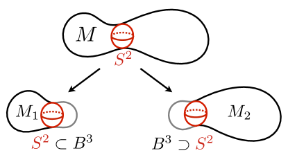
Figure 4: Cutting 3-manifolds along $S^{2}$.

Prime decomposition:

Given two closed 3-manifolds $M_{1}$ and $M_{2}$, we can choose a 3-ball $B^{3}\subset M_{1}$ bounded by an $S^{2}$, and similarly another 3-ball $B^{3}\subset M_{2}$ bounded by an $S^{2}$. We can then paste $M_{1}$ and $M_{2}$ along the common $S^{2}$ to obtain another closed 3-manifold $M$, which is denoted by $M_{1}\#M_{2}$ and is known as the connected sum of $M_{1}$ and $M_{2}$. See Fig. 4. Clearly, $S^{3}$ is the identity under this operation.

A 3-manifold which cannot be written as a connected sum (except with $S^{3}$) is known as a prime manifold. Any 3-manifold $M$ is then known to be given uniquely by a connected sum of prime 3-manifolds,

$$M=M_{1}\#M_{2}\#\cdots\#M_{k}.$$ (3.1)

This is known as the prime decomposition of $M$.

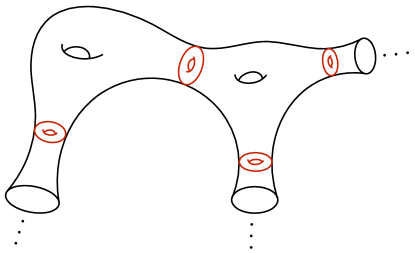
Figure 5: Cutting 3-manifolds along $T^{2}$.

Torus decomposition:

We are now going to cut a prime manifold along embedded $T^{2}$’s, see Fig. 5. In this case, we keep each piece to have torus boundaries, since there are multiple distinct ways to fill in a torus boundary by a solid torus.

One can always cut a manifold $M$ along an embedded torus $T^{2}$ by considering an embedded loop $S^{1}\subset M$ and taking its tubular neighborhood. If $M$ has a torus boundary, we can also cut it along a $T^{2}$ slightly inside the boundary. A manifold $M$ for which the only ways to cut along $T^{2}$ are either of these two trivial methods is called atoroidal.

It is known that we can cut a prime manifold $M$ along copies of $T^{2}$ so that the resulting pieces are all atoroidal. This is the torus decomposition of $M$. In contrast to the prime decomposition, the torus decomposition is known not to be unique, but the non-uniqueness comes only from well-understood examples. These results on prime and torus decompositions were established by [JS79, Joh79].

Atoroidal manifolds:

The next task for us is to understand atoroidal manifolds. Their description follows from the geometrization conjecture of Thurston [Thu82], which states that any 3-manifolds can be cut along $S^{2}$ and $T^{2}$ into pieces which have one of eight possible geometries. In the proof, the Ricci flow of the metric on a given 3-manifold is considered; physically, we consider the RG flow of the sigma model whose target space is the 3-manifold in question. Then, the parts with positive curvature shrink, the parts with negative curvature expand. Shrinking of the positive curvature parts performs the prime decomposition, and then the expansion of the negative curvature parts extracts the hyperbolic manifolds. The remaining connecting parts are shown to be generically either a $T^{2}$ fibration or an $S^{1}$ fibration, all of which are known to have one of the eight geometries, thus proving the conjecture, whose proof had a long and winding history. The overall idea of the proof was first indicated in a series of works by Hamilton e.g. [Ham95], and was later implemented in a series of papers by Perelman starting in [Per02] and completed by subsequent works.

In the context of the torus decomposition, this means that atoroidal manifolds are either i) Seifert manifolds or ii) hyperbolic manifolds. Here, Seifert manifolds are a certain generalization of circle bundles allowing degenerate fibers which we detail below, and hyperbolic manifolds are manifolds of the form $\mathbb{H}^{3}/\Gamma$, where $\mathbb{H}^{3}$ is the three-dimensional hyperbolic space and $\Gamma$ is a discrete subgroup of its isometry group. We note that all hyperbolic manifolds are atoroidal, while not all Seifert manifolds are atoroidal.

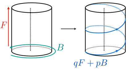
Figure 6: Description of a singular fiber of a Seifert fibration. Instead of filling in $B$, one fills in $qF+pB$.

Seifert manifolds:

In this paper we only consider a subclass of Seifert manifolds. A 3-manifold $M$ in this subclass has a circle action such that its orbits form a two-dimensional surface $\Sigma$. The circle action makes $M$ into a circle bundle on generic points of $\Sigma$, but singular fibers of the following form are allowed.

Namely, starting from an ordinary point in the base $\Sigma$, we consider a neighborhood $D^{2}$. On the solid torus $D^{2}\times S^{1}$, we denote $\partial D^{2}$ by $B$ and the fiber cycle by $F$. Here the cycle $B$ can be shrunk in the geometry. We can instead fill in the torus boundary by a solid torus such that the 1-cycle $pB+qF$ can be shrunk, where $p$ and $q$ are coprime. This operation is known as a Dehn filling. As part of the definition, we demand that $p$ is nonzero. This is to guarantee that the circle action is free. An alternative description consists in gluing back the solid torus $D^{2}\times S^{1}$ by identifying the torus boundaries after performing an $SL(2,\mathbb{Z})$ action, whose explicit form will be given in (3.12).

We note that these operations with $p=1$ do not create a singular fiber. It instead shifts the first Chern class of the circle bundle. Therefore, a Seifert manifold of our interest can be constructed by starting from a trivial $S^{1}$ bundle over a base surface of genus $g$, choosing $k$ points on the base, and performing the Dehn filling operation above the $i$-th point on the base with the parameters $q_{i}/p_{i}$, producing the $i$-th degenerate fiber. We will denote this Seifert manifold by the symbol $(g;q_{1}/p_{1},\ldots,q_{k}/p_{k})$; this is not the standard notation in mathematics literature, but suffices for our purposes. We also note that it is sometimes assumed that $0\leq q_{i}<p_{i}$ to normalize the Seifert parameters. In this paper we do not assume that, and allow arbitrary pairs $(p_{i},q_{i})$ as long as $\mathrm{gcd}(p_{i},q_{i})=1$.

3.2 Associated 3d theories

From the geometric summary above, it is clear that we need to understand the following steps in order to determine the 3d theories obtained by putting $N$ M5-branes on 3-manifolds. Namely, i) we need to understand M5-branes on atoroidal manifolds, And then, ii) we need to understand what happens when we glue two manifolds along $T^{2}$ or $S^{2}$.

Let us discuss the question ii) first. It should be possible to analyze the gluing along $S^{2}$, using the known results concerning the $S^{2}$ reduction of the 6d $\mathcal{N}{=}(2,0)$ theory studied e.g. in [ASNW16]. As this is not the main focus of this paper, we will move on to the gluing along $T^{2}$. Let us review how it goes.

3.2.1 Theories on 3-manifolds with torus boundaries

We need to start by clarifying what is meant by ‘the 6d $\mathcal{N}{=}(2,0)$ theory on 3-manifolds with torus boundaries’, a phrase often used in the context of the 3d/3d correspondence. Close to a $T^{2}$ boundary, the manifold can be approximated as $\mathbb{R}_{>0}\times T^{2}$. Compactifying on $T^{2}$ first, we have 4d $\mathcal{N}{=}4$ $SU(N)$ super Yang–Mills on $\mathbb{R}_{>0}$, where the $SL(2,\mathbb{Z})$ transformation acting on $T^{2}$ is now regarded as the S-duality group action of the $\mathcal{N}{=}4$ super Yang–Mills.

We can give a boundary condition at the boundary of $\mathbb{R}_{>0}$ by choosing a duality frame for the $\mathcal{N}{=}4$ super Yang–Mills, and taking the Dirichlet condition in the chosen frame. This gives rise to an $SU(N)$ flavor symmetry. To choose a duality frame, we need to specify an electric 1-cycle $E$ and a magnetic 1-cycle $M$ on $T^{2}$, forming a basis of $H_{1}(T^{2},\mathbb{Z})$, such that self-dual strings wrapped around $E$ correspond to the W-bosons for the $SU(N)$ flavor symmetry at the boundary. Summarizing, to associate a 3d theory to a 3-manifold with torus boundaries, we need to fix a basis of $H_{1}(T^{2},\mathbb{Z})$ at each boundary.

The necessity of this additional data at the boundary can be understood also as follows. The 6d $\mathcal{N}{=}(2,0)$ theory is a chiral theory and cannot be placed on a space with boundary. To make a closed manifold, we can paste to a torus boundary the product manifold

$$S^{1}\times\text{($D^{2}$ with a full puncture at the origin)}.$$ (3.2)

Then $S^{1}$ is the magnetic 1-cycle $M$ and $\partial D^{2}$ is the electric 1-cycle $E$ in the description above.

We still find it convenient to assign a 3d theory to 3-manifolds with torus boundaries, since such open manifolds commonly appear in the description of classification of 3-manifolds. When we refer to such a 3d theory, we always make a choice of the magnetic 1-cycle $M$ and the electric 1-cycle $E$ at the torus boundary, and implicitly insert the full puncture along the magnetic 1-cycle $M$, shrinking the electric 1-cycle $E$ in the process.

3.2.2 Gluing along $T^{2}$

Given two $T^{2}$ boundaries with the same choice of 1-cycles $E$ and $M$, we can simply glue them by gauging the diagonal combination of two $SU(N)$ symmetries associated to the two $T^{2}$ boundaries by 3d $\mathcal{N}{=}4$ $SU(N)$ vector multiplet. In order to glue two $T^{2}$ boundaries with two different choices of pairs of 1-cycles $E$ and $M$, we need to perform the $SL(2,\mathbb{Z})$ transformation first. Any $SL(2,\mathbb{Z})$ transformation can be done by a sequence of $S$ and $T$ transformations given by

$$S=\begin{pmatrix}0&-1\\ 1&0\end{pmatrix},\qquad T=\begin{pmatrix}1&1\\ 0&1\end{pmatrix},$$ (3.3)

whose manifestation as operations on 3d supersymmetric theories was determined in [GW08a, GW08b]. Namely, the $S$ transformation is realized by coupling to the duality wall theory $T(SU(N))$, and the $T$ transformation is realized by shifting the Chern–Simons level of the $SU(N)$ flavor background by one.

The $S$ transformation preserves 3d $\mathcal{N}{=}4$ supersymmetry, while the $T$ transformation preserves only 3d $\mathcal{N}{=}3$ supersymmetry, since it involves the supersymmetric Chern–Simons coupling. Therefore, gluing with an arbitrary $SL(2,\mathbb{Z})$ transformation always preserves at least 3d $\mathcal{N}{=}3$ supersymmetry.

3.2.3 Ingredients

Now that we have some understanding of the gluing operations, we need to understand the ingredients we glue, i.e. theories associated to atoroidal manifolds. As reviewed above, atoroidal manifolds are either hyperbolic manifolds or Seifert manifolds, which we discuss in turn.

Theories on hyperbolic manifolds:

The 3d theories obtained by putting two M5-branes on hyperbolic manifolds were the focus of the epoch-making paper [DGG11a, DGG11b]. The theories constructed in these original papers, however, associates a $U(1)$ flavor symmetry for each $T^{2}$ boundary, rather than an $SU(2)$ flavor symmetry, which we expect on general grounds. Such theories with an $SU(2)$ flavor symmetry per $T^{2}$ boundary were later studied in [CDGS14, GY18a]. The generalization to more than two M5-branes has also been studied, starting in [DGG13].

Theories on Seifert manifolds:

The 3d theories obtained by putting $N$ M5-branes on Seifert manifolds have also been determined previously, see e.g. [GGP13, CDGS14, PY15, GPV16, GPPV17, EKSNW19, CGK20], although the determination was usually a byproduct rather than the main topic of these papers. Here we give a brief summary of the construction.

As recalled above, Seifert manifolds of our interest are obtained by starting from a direct product of $S^{1}$ and a surface $\Sigma$ with boundaries, and performing a Dehn filling for each of its boundaries. A Dehn filling is done by gluing an $S^{1}\times D^{2}$ after an appropriate $SL(2,\mathbb{Z})$ transformation. As $D^{2}$ is also a special case of a surface with boundaries, all that is left is to understand the 3d theory obtained by putting $N$ M5-branes on a product $S^{1}\times\Sigma$, with $\Sigma$ a surface with $m$ boundaries $\partial\Sigma=C_{1}\cup\cdots\cup C_{m}$.

Theories on $S^{1}\times\Sigma$:

Let us first pick $C_{i}$ to be the electric cycle and the $S^{1}$ fiber to be the magnetic cycle. Equivalently, let us fill in $C_{i}$ by a disk $D^{2}_{i}$ with a full puncture at the origin. We then have $N$ M5-branes on a product $S^{1}$ times a sphere $S^{2}$ with $m$ full punctures. This then gives the $T_{N,m}$ theory we already used in Sec. 2.2.1.

Secondly, we can choose $C_{i}$ to be the magnetic cycle and the $S^{1}$ fiber to be the electric cycle. Equivalently, let us fill in $S^{1}$ of each boundary $S^{1}\times C_{i}$ by a $D^{2}$, again with a full puncture at the origin. The two ways of filling are related by the S-transformation at each boundary, and it is known that the second method leads to the 3d ‘theory’ which is simply the diagonal Dirichlet boundary condition setting all $SU(N)$ flavor symmetries associated to $m$ boundaries the same [BTX10, Sec. 5.2]. These two descriptions are related by the 3d mirror symmetry. Summarizing, the $T_{N,m}$ theory is given by taking $m$ copies of $T(SU(N))$ theories with $SU(N)^{(i)}_{H}\times SU(N)_{C}^{(i)}$ flavor symmetry, for $i=1,\ldots,m$, and gauging the diagonal subgroup $SU(N)_{C}$ of $SU(N)_{C}^{(1,\ldots,m)}$. We illustrate the case of $T_{N}=T_{N,3}$ in Fig. 7. The genus-$g$ version is known to be obtained simply by adding $g$ adjoint hypermultiplets when we gauge $SU(N)_{C}$. We denote the resulting theory by $T_{N,m,g}$.

$$\leavevmode\hbox to27.09pt{\vbox to23.51pt{\text{[drawing]}}}=\leavevmode\hbox to70.88pt{\vbox to82.19pt{\text{[drawing]}}} T_{N} 0 S S S T_{N} 0 S S S$$

Figure 7: The 3d mirror of the $T_{N}$ theory is obtained by taking three copies of $T(SU(N))$ theory and gauge its diagonal $SU(N)$ symmetry. The circle with zero in it symbolizes the gauging with zero Chern–Simons level, i.e. the $\mathcal{N}{=}4$ gauging.

We can use this description of the $T_{N,m,g}$ theory to derive our crucial chiral ring relation (2.13), using some basic properties of the $T(SU(N))$ theory. Denote the moment map fields of its $SU(N)_{H}$ and $SU(N)_{C}$ flavor symmetries by $\mu_{H}$ and $\mu_{C}$ respectively. Let us couple $T(SU(N))$ with adjoint scalar fields $\Phi_{C}$, $\Phi_{H}$ via

$$W=\mathop{\mathrm{tr}}\Phi_{H}\mu_{C}+\mathop{\mathrm{tr}}\Phi_{C}\mu_{H}.$$ (3.4)

Then the following crucial chiral ring relations:

$$\mathop{\mathrm{tr}}(\Phi_{H})^{n}=\mathop{\mathrm{tr}}(\mu_{H})^{n},\qquad\mathop{\mathrm{tr}}(\Phi_{C})^{n}=\mathop{\mathrm{tr}}(\mu_{C})^{n}$$ (3.5)

are satisfied for arbitrary $n$.

One way to derive these relations is to realize the $T(SU(N))$ theory as 4d $\mathcal{N}{=}4$ super-Yang–Mills on a segment with suitable boundary conditions, as in [GW08b]. The undeformed $T(SU(N))$ theory is known to be the S-dual of the Nahm pole boundary condition

$$\phi(x)\sim\frac{\nu}{x}$$ (3.6)

where $x$ is the distance to the boundary, $\nu$ is the principal nilpotent element in $\mathfrak{su}(N)$, and $\sim$ denotes that the two are conjugate. As $\phi(x)$ at the other boundary $x=x_{0}$ is identified with $\mu_{H}$, we see that $\mathop{\mathrm{tr}}(\mu_{H})^{n}=0$ for all $n$.

A nonzero diagonalizable $\Phi_{H}$ is known to deform this Nahm pole boundary condition to the form

$$\phi(x)\sim\Phi_{H}+\frac{\nu^{\prime}}{x},$$ (3.7)

where $\nu^{\prime}$ is now the principal nilpotent element in the commutant of $\Phi_{H}$ in $\mathfrak{su}(N)$. From this we see $\mathop{\mathrm{tr}}(\Phi_{H})^{n}=\mathop{\mathrm{tr}}(\mu_{H})^{n}$ for all $n$. The equation $\mathop{\mathrm{tr}}(\Phi_{C})^{n}=\mathop{\mathrm{tr}}(\mu_{C})^{n}$ follows perfectly analogously.

With this property of the $T(SU(N))$ theory in hand, it is a simple matter to derive the chiral ring relation (2.13). The $T_{N,m}$ theory is given by taking $m$ copies of the $T(SU(N))$ theory and coupling them to a single $\mathcal{N}{=}4$ $SU(N)$ vector multiplet, with the superpotential

$$W=\sum_{i}\mathop{\mathrm{tr}}\Phi\mu_{C}^{(i)},$$ (3.8)

where $\Phi$ is now dynamical. This immediately implies

$$\mathop{\mathrm{tr}}(\mu_{H}^{(i)})^{k}=\mathop{\mathrm{tr}}\Phi^{k},$$ (3.9)

independent of $i$ for all $k$. As $\mu_{H}^{(i)}$ are identified as the moment map field $\mu_{i}$ of the $i$-th $SU(N)$ of the $T_{N,m}$ theory, we derived (2.13), that is,

$$\text{$\mathop{\mathrm{tr}}(\mu_{i})^{2}$ is independent of $i$}.$$ (3.10)

Dehn fillings:

To complete our description of the basic operations, let us briefly discuss how to perform the Dehn fillings of a torus boundary. Geometrically, it is done by pasting $S^{1}\times D^{2}$ along the torus boundary. We can associate multiple 3d theories to $S^{1}\times D^{2}$ related by $SL(2,\mathbb{Z})$ operations depending on the choice of a basis of $H_{1}(T^{2},\mathbb{Z})$ at its boundary. Equivalently, these are obtained by pasting $S^{1}\times D^{2}$ and $S^{1}\times(\text{$D^{2}$ with a full puncture})$ with $SL(2,\mathbb{Z})$ operations along their torus boundaries.

These are the special $m=1$ case of what we just discussed above. In particular, when the $SL(2,\mathbb{Z})$ operation is trivial, the 3d manifold is $S^{1}\times S^{2}$ with a full puncture wrapping $S^{1}$, and the associated theory is $T(SU(N))$ with one of its $SU(N)$ symmetry gauged. This is the $T_{N,1}$ theory. In contrast, when we use the $S$ operation, the 3d manifold is $S^{3}$, with a full puncture wrapping a circle fiber of its Hopf fibration. This is a rather degenerate setup, and simply gives a free boundary condition to the background fields of the $SU(N)$ flavor symmetry supported on the puncture.

In the language of the electric/magnetic 1-cycle chosen at the torus boundary, this means that filling in the magnetic cycle is simply done by gauging the $SU(N)$ flavor symmetry with an $\mathcal{N}{=}4$ vector multiplet, and that filling in the electric cycle is done by coupling it to the $T_{N,1}$ theory, again via an $\mathcal{N}{=}4$ $SU(N)$ vector multiplet.

3.3 Main examples from geometry

As an example, let us consider the 3d theory associated to a Seifert bundle over $S^{2}$ with three singular fibers, with Seifert parameters $1/k_{1,2,3}$, respectively. This manifold is obtained by first considering $S^{1}$ times $S^{2}$ with three holes whose boundaries we denote by $C_{1,2,3}$, and Dehn-filling three torus boundaries by filling the direction $F+k_{i}C_{i}$ where $F$ is the fiber $S^{1}$ direction.

As discussed, the 3d $T_{N}$ theory corresponds to the choice of $F$ as the magnetic 1-cycle and $C_{i}$ as the electric 1-cycle. For the solid torus $S^{1}\times D^{2}$, we define (perhaps surprisingly) $C^{\prime}=S^{1}$ and $F^{\prime}=\partial D^{2}$. We then specify the gluing in terms of the $SL(2,\mathbb{Z})$ matrix $g$ appearing in the relation

$$(C,F)g=(C^{\prime},F^{\prime}).$$ (3.11)

This somewhat peculiar convention of ours is designed so that the Dehn filling with the identity element $1\in SL(2,\mathbb{Z})$ is done by a simple gauging of the $SU(N)$ flavor symmetry.

In our case we have $g=T^{k_{i}}$, which simply adds the level $k_{i}$ Chern–Simons coupling. This means that the resulting 3d theory is the $T_{N}$ theory whose three $SU(N)$ flavor symmetries are gauged with 3d $\mathcal{N}{=}3$ Chern–Simons coupling $k_{i}$.

Another description is as follows. We need to perform Dehn fillings at the three torus boundaries. Our choice of the Seifert parameters means that at the $i$-th boundary, we perform the $SL(2,\mathbb{Z})$ operation $T^{k_{i}}S$, before gluing in the $T_{N,1}$ theory. As the $T_{N,1}$ theory is itself the $T(SU(N))$ theory with $SU(N)_{C}$ gauged, two $S$ operations cancel, and we end up simply gauging the $i$-th $SU(N)$ flavor symmetry of the $T_{N}$ theory with the $\mathcal{N}{=}3$ Chern–Simons term with the level $k_{i}$.

More generally, when the Seifert parameters are $q_{i}/p_{i}$, one needs to perform an appropriate $SL(2,\mathbb{Z})$ transformation to bring the cycle $q_{i}F+p_{i}C_{i}$ to be shrunk into the magnetic 1-cycle. This can be done by the transformation

$$g=T^{k^{(1)}}ST^{k^{(2)}}S\cdots ST^{k^{(a-1)}}ST^{k^{(a)}}$$ (3.12)

where the Chern–Simons levels $k^{(t)}$ for $t=1,2,\ldots,a$ is given by a continued fraction expansion of the Seifert parameters, i.e. by

$$\frac{q}{p}=\dfrac{1}{k^{(1)}-\dfrac{1}{k^{(2)}-\dfrac{1}{k^{(3)}-\cdots}}}.$$ (3.13)

Note that we dropped the subscript $i$ to specify the singular fiber considered, to lighten the notation somewhat.

Figure 8: The 3d theory associated to the Seifert bundle over $S^{2}$ with three singular fibers. For the notation, see the main text.

Summarizing, we see that the 3d theory obtained from the Seifert bundle over $S^{2}$ with three punctures with parameters $q_{i}/p_{i}$ has the form given in Fig. 8. There, a circle enclosing $k$ denotes an $\mathcal{N}{=}3$ Chern–Simons vector multiplet with level $k$, a hexagon is the 3d $T_{N}$ theory, and a box with an $S$ denotes the 3d $T(SU(N))$ theory. This is a well-known result [GGP13, PY15, GPV16, GPPV17, EKSNW19, CGK20], although the generic presence of $\mathcal{N}{=}3$ supersymmetry was not explicitly remarked in those papers.

In the simplest case when $q_{i}/p_{i}=1/k_{i}$, these are exactly the theories considered in Sec. 2.2.1, where we saw that the supersymmetry enhances to $\mathcal{N}{=}4$ when $1/k_{1}+1/k_{2}+1/k_{3}=0$. Our question now is whether we can understand this enhancement geometrically. To study this question, we need to come back to a general question on how the geometry determines the amount of supersymmetries preserved.

3.4 Number of supersymmetries from the geometry

The 6d theory on M5-branes has the R-symmetry $Sp(2)_{R}\simeq SO(5)_{R}$. A generic 3-manifold $M$ has holonomies in $SO(3)$. We can turn the R-symmetry background on $M$, by embedding the $SO(3)$ spin connection into the R-symmetry by

$$SO(3)\subset SO(3)\times SO(2)\subset SO(5)_{R}.$$ (3.14)

A short computation reveals that two supercharges remain, realizing 3d $\mathcal{N}{=}2$ supersymmetry.

As another example, let us suppose the 3-manifold $M$ is a product $S^{1}\times\Sigma$. As is well-known, M5-branes on $\Sigma$ give a 4d $\mathcal{N}{=}2$ theory, and a further compactification on $S^{1}$ gives a 3d $\mathcal{N}{=}4$ theory. More generally, any 3-manifold $M$ whose holonomies are in $SO(2)$ gives rise to a 3d $\mathcal{N}{=}4$ theory. Indeed, we can turn the R-symmetry background on $M$ by embedding the $SO(2)$ spin connection to the R-symmetry by

$$SO(2)\subset SO(5)_{R}.$$ (3.15)

Again a short computation reveals that four supercharges remain, realizing 3d $\mathcal{N}{=}4$ supersymmetry.

Therefore, a way to look for the cause of the $\mathcal{N}{=}4$ enhancements is to study when a 3-manifold has a reduced holonomy in $SO(2)$. A simple result which is crucial to us is the following statement: Theorem: A Seifert manifold of type $(g;q_{1}/p_{1},\ldots,q_{m}/p_{m})$ in our notation is, unless $g=0$ and $m<3$, an order-$n$ quotient of an $S^{1}$ fibration over a Riemann surface $\Sigma$, where $n=\mathrm{lcm}\,\{p_{i}\}$ and the first Chern class of the $S^{1}$ fibration is $n\sum q_{i}/p_{i}$. The quotient is given by an order-$n$ isometry of $\Sigma$ combined with a $1/n$ rotation of the fiber. This theorem follows from e.g. Lemma 3.7 of [Sco83], where the same statement is proved except that the quotient can be taken to be an isometry. That the quotient can be taken to be an isometry follows by first considering an arbitrary metric and then averaging it over the quotient group.

Now, this theorem in particular implies that a Seifert manifold of type $(g;q_{1}/p_{1},\ldots,q_{k}/p_{k})$ is an order-$n$ quotient of a trivial product $\Sigma\times S^{1}$ when $\sum_{i}q_{i}/p_{i}=0$. As the quotient process in this case does not affect the holonomy group $SO(2)$, we see that the 3d theories associated to this class of Seifert manifolds should have an enhanced $\mathcal{N}{=}4$ supersymmetry when $\sum_{i}q_{i}/p_{i}=0$.

This gives a geometric explanation of the $\mathcal{N}{=}4$ supersymmetry of the theories we introduced in Sec. 2.2.1, namely the $T_{N}$ theory gauged with $SU(N)^{3}$ with levels $k_{1,2,3}$ when $1/k_{1}+1/k_{2}+1/k_{3}=0$. This is because, as we saw in the subsection above, they come from Seifert manifolds of type $(0;1/k_{1},1/k_{2},1/k_{3})$. This analysis can be easily generalized to the $T_{N,m,g}$ theory whose $SU(N)^{m}$ symmetry is gauged with Chern–Simons levels $k_{i}$. It enhances to $\mathcal{N}{=}4$ when $\sum 1/k_{i}=0$. This agrees with the geometric theorem quoted above, since the corresponding Seifert manifold is of type $(g;1/k_{i})$.

Our geometric analysis also predicts that the 3d theories given in Sec. 3.3 should have an enhanced $\mathcal{N}{=}4$ supersymmetry when $\sum q_{i}/p_{i}=0$. This is the task we would like to investigate next. Before that, we need to establish a field-theoretical result first.

3.5 A field-theoretical interlude

3.5.1 The statement to be established

Figure 9: A single chain of $T(SU(N))$ theories coupled by $\mathcal{N}{=}3$ Chern–Simons multiplets.

To analyze the theory depicted in Fig. 8, the part essential to us is the chain structure shown in Fig. 9 implementing an $SL(2,\mathbb{Z})$ transformation $g$. There, the lines connecting to $\mu$ and $\mu^{\prime}$ on the extreme left and right signify that the first and the last $\mathcal{N}{=}3$ Chern–Simons multiplets also couple to these complex adjoint scalar fields, and the Chern–Simons levels $k^{(i)}$ are determined in terms of the continued fraction expansion

$$\frac{q}{p}=\dfrac{1}{k^{(1)}-\dfrac{1}{k^{(2)}-\dfrac{1}{k^{(3)}-\cdots}}}$$ (3.16)

as before. We note that $g$ has the form

$$g=T^{k^{(1)}}ST^{k^{(2)}}S\cdots ST^{k^{(a)}}=\begin{pmatrix}q^{\prime}&p\\ r&q\end{pmatrix}$$ (3.17)

where

$$\frac{q^{\prime}}{p}=\dfrac{1}{k^{(a)}-\dfrac{1}{k^{(a-1)}-\dfrac{1}{k^{(a-2)}-\cdots}}}.$$ (3.18)

Let us denote by $\mu_{C,H}^{(i)}$ the Coulomb-branch and Higgs-branch moment map fields of the $i$-th $T(SU(N))$ theory, and by $\Phi^{(i)}$ the adjoint scalar of the $i$-th Chern–Simons multiplet. The superpotential is then given by

$$W=\sum_{i=1}^{a}\left(\mathop{\mathrm{tr}}\mu_{H}^{(i-1)}\Phi^{(i)}-\frac{k^{(i)}}{2}\mathop{\mathrm{tr}}(\Phi^{(i)})^{2}+\mathop{\mathrm{tr}}\Phi^{(i)}\mu_{C}^{(i)}\right)$$ (3.19)

where $\mu_{H}^{(0)}:=\mu$ and $\mu_{C}^{(a)}:=\mu^{\prime}$.

We now show the following statement inductively in terms of the length $a$ of the chain: Statement: The effective superpotential is equivalent to $$W=\frac{1}{2}\frac{q}{p}\mathop{\mathrm{tr}}\mu^{2}+\sum_{i=1}^{a}c^{(i)}\mathop{\mathrm{tr}}\mu_{H}^{(i-1)}\mu_{C}^{(i)}+\frac{1}{2}\frac{q^{\prime}}{p}\mathop{\mathrm{tr}}(\mu^{\prime})^{2},$$ (3.20) after eliminating $\Phi^{(j)}$. Here, $c^{(i)}$ are certain constants satisfying $$\prod c^{(i)}=1/p.$$ (3.21) Those readers who are not interested in the (rather technical) derivation can skip to the beginning of the next section 3.6.

3.5.2 A lemma and a corollary

Before we start the derivation of the statement above, we need the following lemma: Lemma: For a single $T(SU(N))$ theory, the deformation $$W=\mathop{\mathrm{tr}}\Phi\mu_{C}+\mathop{\mathrm{tr}}\mu_{H}\Phi^{\prime}+\frac{a}{2}\mathop{\mathrm{tr}}(\mu_{H})^{2},$$ (3.22) and the deformation $$W=\frac{a}{2}\mathop{\mathrm{tr}}\Phi^{2}+\mathop{\mathrm{tr}}\Phi\mu_{C}+\mathop{\mathrm{tr}}\mu_{H}\Phi^{\prime}$$ (3.23) are equivalent at finite nonzero $a$, where $\Phi$ and $\Phi^{\prime}$ are background superfields. To show this, we consider how the chiral ring relation at $a=0$,

$$\mathop{\mathrm{tr}}\Phi^{2}=\mathop{\mathrm{tr}}(\mu_{H})^{2}$$ (3.24)

which we already recalled at (3.5), would be deformed under the first deformation (3.22) at nonzero $a$. We assign $\mathcal{N}{=}2$ R-charge $+1$ to $\Phi$, $\Phi^{\prime}$, $\mu_{C,H}$; we also assign the $J_{34}$ charge $+1$ to $\Phi$, $\mu_{H}$ and $-1$ to $\Phi^{\prime}$, $\mu_{C}$. Then $a$ has the R-charge $0$ and the $J_{34}$-charge $-2$. As the equation has the R-charge $2$ and the $J_{34}$-charge $2$, the only term one can write is $a^{-2}$ times a quadratic combination of $\Phi^{\prime}$ and $\mu_{C}$. This is forbidden, since the chiral ring relation should be continuous at $a=0$. This establishes that the relation (3.24) holds unchanged under the deformation (3.22) at finite $a$. This means that the deformation (3.22) is equivalent to

$$W=\frac{\epsilon}{2}\mathop{\mathrm{tr}}\Phi^{2}+\mathop{\mathrm{tr}}\Phi\mu_{C}+\mathop{\mathrm{tr}}\mu_{H}\Phi^{\prime}+\frac{1}{2}(a-\epsilon)\mathop{\mathrm{tr}}(\mu_{H})^{2}$$ (3.25)

for an infinitesimal $\epsilon$. This implies that it is further equivalent to (3.23) and concludes the derivation of the lemma.

Let us now add a term $\mathop{\mathrm{tr}}\tilde{\Phi}\Phi-\frac{k}{2}\mathop{\mathrm{tr}}\Phi^{2}$ to both (3.22) and (3.23), integrate out $\Phi$, and replace the resulting $\tilde{\Phi}$ by $\Phi$ since the original $\Phi$ no longer appears. We immediately obtain the following corollary: Corollary: For a single $T(SU(N))$ theory, the deformation $$W^{\prime}=\frac{1}{2k}\mathop{\mathrm{tr}}(\Phi+\mu_{C})^{2}+\frac{a}{2}\mathop{\mathrm{tr}}(\mu_{H})^{2}+\mathop{\mathrm{tr}}\mu_{H}\Phi^{\prime}$$ (3.26) and $$W^{\prime}=\frac{1}{2(k-a)}\mathop{\mathrm{tr}}(\Phi+\mu_{C})^{2}+\mathop{\mathrm{tr}}\mu_{H}\Phi^{\prime}$$ (3.27) are equivalent at finite nonzero $a$ and $k$, where $\Phi$ and $\Phi^{\prime}$ are background superfields.

We note that the lemma and the corollary only guarantee that the two deformations are equivalent up to $\bar{D}_{\dot{\alpha}}$-exact terms. In the case we encounter below, $\Phi$ and $\Phi^{\prime}$ are either chiral primaries from SCFTs other than the $T(SU(N))$ theory in question. Therefore, the $\bar{D}_{\dot{\alpha}}$-exact terms are actually absent. The same can also be said when we actually use the corollary.

3.5.3 Derivation

Let us begin the derivation of the statement itself. The case when the length is $1$ is immediate. Let us then assume that this statement has been shown up to the length $a-1$. We see that the superpotential is equivalent to

$$W=\frac{1}{2k^{(1)}}\mathop{\mathrm{tr}}(\mu+\mu_{C}^{(1)})^{2}+\frac{1}{2}\frac{\tilde{q}}{\tilde{p}}\mathop{\mathrm{tr}}(\mu_{H}^{(1)})^{2}+\sum_{i=2}^{a}c^{(i)}\mathop{\mathrm{tr}}\mu_{H}^{(i-1)}\mu_{C}^{(i)}+\frac{1}{2}\frac{\tilde{q}^{\prime}}{\tilde{p}}\mathop{\mathrm{tr}}(\mu^{\prime})^{2}$$ (3.28)

where

$$\tilde{g}=T^{k^{(2)}}S\cdots ST^{k^{(a)}}=\begin{pmatrix}\tilde{q}^{\prime}&\tilde{p}\\ \tilde{r}&\tilde{q}\end{pmatrix}.$$ (3.29)

Applying the corollary above, we can rewrite $W$ as

$$W=\frac{1}{2}\frac{q}{p}\mathop{\mathrm{tr}}(\mu+\mu_{C}^{(1)})^{2}+\sum_{i=2}^{a}c^{(i)}\mathop{\mathrm{tr}}\mu_{H}^{(i-1)}\mu_{C}^{(i)}+\frac{1}{2}\frac{\tilde{q}^{\prime}}{\tilde{p}}\mathop{\mathrm{tr}}(\mu^{\prime})^{2}$$ (3.30)

where we used $p/q=k^{(1)}-\tilde{q}/\tilde{p}$. We now repeatedly use the lemma applied to the $i$-th $T(SU(N))$ theory, and perform the following replacement of the superpotential deformations:

$$\mathop{\mathrm{tr}}(\mu_{C}^{(i)})^{2}\leftrightarrow(c^{(i+1)})^{2}\mathop{\mathrm{tr}}(\mu_{C}^{(i+1)})^{2}.$$ (3.31)

More explicitly, we do the exchanges

$$\frac{1}{2}\frac{q}{p}\mathop{\mathrm{tr}}(\mu_{C}^{(1)})^{2}\leftrightarrow\frac{1}{2}\frac{q}{p}(c^{(2)})^{2}\mathop{\mathrm{tr}}(\mu_{C}^{(2)})^{2}\leftrightarrow\frac{1}{2}\frac{q}{p}(c^{(2)}c^{(3)})^{2}\mathop{\mathrm{tr}}(\mu_{C}^{(3)})^{2}\\ \leftrightarrow\cdots\leftrightarrow\frac{1}{2}\frac{q}{p}\left(\prod_{i=2}^{a}c^{(a)}\right)^{2}\mathop{\mathrm{tr}}(\mu^{\prime})^{2}=\frac{1}{2}\frac{q}{p}\frac{1}{\tilde{p}^{2}}\mathop{\mathrm{tr}}(\mu^{\prime})^{2}$$ (3.32)

where we used the inductive assumption in the last equality. This allows us to rewrite (3.30) further to

$$W=\frac{1}{2}\frac{q}{p}\mathop{\mathrm{tr}}\mu^{2}+\frac{q}{p}\mathop{\mathrm{tr}}\mu\mu_{C}^{(1)}+\sum_{i=2}^{a}c^{(i)}\mathop{\mathrm{tr}}\mu_{H}^{(i-1)}\mu_{C}^{(i)}+\frac{1}{2}\left(\frac{q}{p}\frac{1}{\tilde{p}^{2}}+\frac{\tilde{q}^{\prime}}{\tilde{p}}\right)\mathop{\mathrm{tr}}(\mu^{\prime})^{2}.$$ (3.33)

As

$$\begin{pmatrix}q^{\prime}&p\\ r&q\end{pmatrix}=T^{k^{(1)}}S\begin{pmatrix}\tilde{q}^{\prime}&\tilde{p}\\ \tilde{r}&\tilde{q}\end{pmatrix},$$ (3.34)

we have

$$q=\tilde{p},\qquad r=\tilde{q}^{\prime}.$$ (3.35)

Using these relations, we finally find that

$$W=\frac{1}{2}\frac{q}{p}\mathop{\mathrm{tr}}\mu^{2}+\sum_{i=1}^{a}c^{(i)}\mathop{\mathrm{tr}}\mu_{H}^{(i-1)}\mu_{C}^{(i)}+\frac{1}{2}\frac{q^{\prime}}{p}\mathop{\mathrm{tr}}(\mu^{\prime})^{2},$$ (3.36)

with

$$\prod_{i=1}^{a}c^{(i)}=1/p,$$ (3.37)

which is exactly the property we wanted to demonstrate for the length $a$ chain. We make a further remark on the $SL(2,\mathbb{Z})$ duality wall theory in Appendix C, using the Statement established above.

3.6 Supersymmetry enhancements accounted for by holonomy

We now analyze the structure of the theory shown in Fig. 8. Namely, we take three tails of the form discussed in (3.20), and couple them to a $T_{N}$ theory. After eliminating the adjoint scalars in the $\mathcal{N}{=}3$ Chern–Simons multiplets, we have the superpotential of the form

$$W= \frac{1}{2}\frac{q_{1}}{p_{1}}\mathop{\mathrm{tr}}(\mu_{1})^{2}+\frac{q_{1}}{p_{1}}\mathop{\mathrm{tr}}\mu_{1}\mu_{1,C}^{(1)}+\sum_{i=2}^{a_{1}-1}c_{1}^{(i)}\mathop{\mathrm{tr}}\mu_{1,H}^{(i-1)}\mu_{1,C}^{(i)}$$ (3.38)

$$+\frac{1}{2}\frac{q_{2}}{p_{2}}\mathop{\mathrm{tr}}(\mu_{2})^{2}+\frac{q_{2}}{p_{2}}\mathop{\mathrm{tr}}\mu_{2}\mu_{2,C}^{(1)}+\sum_{i=2}^{a_{2}-1}c_{2}^{(i)}\mathop{\mathrm{tr}}\mu_{2,H}^{(i-1)}\mu_{2,C}^{(i)}$$

$$+\frac{1}{2}\frac{q_{3}}{p_{3}}\mathop{\mathrm{tr}}(\mu_{3})^{2}+\frac{q_{3}}{p_{3}}\mathop{\mathrm{tr}}\mu_{3}\mu_{2,C}^{(1)}+\sum_{i=2}^{a_{3}-1}c_{3}^{(i)}\mathop{\mathrm{tr}}\mu_{3,H}^{(i-1)}\mu_{3,C}^{(i)}.$$

Using $\mathop{\mathrm{tr}}(\mu_{1})^{2}=\mathop{\mathrm{tr}}(\mu_{2})^{2}=\mathop{\mathrm{tr}}(\mu_{3})^{2}$, we find that the superpotential simplifies further when

$$\frac{q_{1}}{p_{1}}+\frac{q_{2}}{p_{2}}+\frac{q_{3}}{p_{3}}=0$$ (3.39)

to

$$W= \frac{q_{1}}{p_{1}}\mathop{\mathrm{tr}}\mu_{1}\mu_{1,C}^{(1)}+\sum_{i=2}^{a_{1}-1}c_{1}^{(i)}\mathop{\mathrm{tr}}\mu_{1,H}^{(i-1)}\mu_{1,C}^{(i)}$$ (3.40)

$$+\frac{q_{2}}{p_{2}}\mathop{\mathrm{tr}}\mu_{2}\mu_{2,C}^{(1)}+\sum_{i=2}^{a_{2}-1}c_{2}^{(i)}\mathop{\mathrm{tr}}\mu_{2,H}^{(i-1)}\mu_{2,C}^{(i)}$$

$$+\frac{q_{3}}{p_{3}}\mathop{\mathrm{tr}}\mu_{3}\mu_{2,C}^{(1)}+\sum_{i=2}^{a_{3}-1}c_{3}^{(i)}\mathop{\mathrm{tr}}\mu_{3,H}^{(i-1)}\mu_{3,C}^{(i)}.$$

We now consider the R-charge $J_{34}$ of the $\mathcal{N}{=}4$ system of one $T_{N}$ theory and many copies of $T(SU(N))$ theory before the coupling to $\mathcal{N}{=}3$ Chern–Simons multiplets. This assigns charge $+2$ to the moment map fields on the Higgs branch side, and to $-2$ to those on the Coulomb branch side. Our final superpotential (3.40) when the condition (3.39) is satisfied preserves $J_{34}$, and therefore the supersymmetry of the gauged theory enhances to $\mathcal{N}{=}4$ when the condition (3.39) is satisfied.

It is clear that this analysis can be extended to the 3d theories associated to Seifert manifolds of type $(g;q_{i}/p_{i})$. All what is needed is to replace the $T_{N}$ theory with the $T_{N,m,g}$ theory, which has moment map fields $\mu_{i}$ for $i=1,\ldots,m$ such that $\mathop{\mathrm{tr}}(\mu_{i})^{2}$ is independent of $i$. Then, the effective superpotential after eliminating adjoint chiral superfields preserves $J_{34}$ if and only if $\sum q_{i}/p_{i}=0$, showing $\mathcal{N}{=}4$ enhancements. This is in accord with the geometric criterion we quoted in Sec. 3.4.

3.7 Supersymmetry enhancements unaccounted for by holonomy

Let now briefly come back to the theories we discussed in Sec. 2.2.2, shown in Fig. 2 and in Fig. 3. These theories are obtained by taking copies of 3d $T_{N}$ theories and coupling them via $\mathcal{N}{=}3$ Chern–Simons multiplets.

According to our discussion in Sec. 3.2, such theories come from the compactification of $N$ M5-branes on a 3-manifold, since the $T_{N}$ theory comes from $N$ M5-branes on $S^{1}$ times a sphere with three holes, and coupling them via $\mathcal{N}{=}3$ Chern–Simons multiplets can be realized by gluing them via appropriate $T$ transformations. For example, the theory shown in Fig. 2 comes from the geometry shown in Fig. 10. Here it would be useful to recall our convention for the $SL(2,\mathbb{Z})$ transformation. On the $i$-th boundary, we call $F$ the $S^{1}$ fiber and $C$ the boundary on the base surface. Let $(C,F)$ be these 1-cycles on the left hand side and $(C^{\prime},F^{\prime})$ be defined analogously on the right hand side. Then we have

$$(C,F)g=(C^{\prime},F^{\prime}).$$ (3.41)

Figure 10: A geometry generating the theory given in Fig. 2.

We saw in Sec. 2.2.2 that these theories have an enhanced $\mathcal{N}{=}4$ supersymmetry when

$$\frac{1}{k_{1}}+\frac{1}{k_{2}}+\frac{1}{k_{3}}=0$$ (3.42)

The holonomy of the manifold stays the generic $SO(3)$ even when the condition (3.42) is satisfied. An argument for this is as follows. First of all we recall that $SO(2)$ holonomy is equivalent to the existence of a covariantly constant vector field; by [WJ86, Th. 3], a compact manifold with such a vector is covered by $S^{1}\times\Sigma$. But now we argue that a graph manifold which is not Seifert cannot be covered by a Seifert (such as $S^{1}\times\Sigma$). Given a covering $\tilde{M}\to M$, if $\tilde{M}$ is modelled on one of the eight Thurston geometries (mentioned at the beginning of this section), then $M$ is also modelled on the same geometry [Mar16, Cor. 12.9.5]. In particular, if $\tilde{M}=S^{1}\times\Sigma$ covers a manifold $M$, then $M$ has the same geometry of $S^{1}\times\Sigma$, and so in particular it is Seifert.

What is left to be shown is that our graph manifold, shown in Fig. 10, is not a Seifert manifold in disguise. For Seifert manifolds, every essential surface is either horizontal or vertical with respect to the fibration [Mar16, Proposition 10.4.9]. Now, each of the three $T^{2}$ where we glue two parts is an essential torus. If the whole manifold were a Seifert, each of these tori would be either horizontal or vertical with respect to the fibration. If it is vertical, then the two fibrations on the two pieces glue well along these $T^{2}$, which is true only when $k_{1}=k_{2}=k_{3}=0$. If it is horizontal, the fibers need to lie in intervals in the two pieces. But this is impossible, because if it is horizontal then its complement is a simple $\mathbb{R}$-bundle, which is not the case.

As a consequence, our graph manifold has $SO(3)$ holonomy; geometrically we would then only expect $\mathcal{N}{=}2$ supersymmetry, leaving the supersymmetry enhancement unaccounted for.

Figure 11: A further generalization of Fig. 10.

Figure 12: The 3d theory associated to the 3-manifold given in Fig. 11. The second one is obtained by applying the 3d mirror symmetries to the two $T_{N}$ theories involved.

We can make a further generalization by using a general $SL(2,\mathbb{Z})$ element $g_{i}$ instead of $T^{k_{i}}$ in Fig. 10, as shown in Fig. 11, whose field-theoretical realization is given in Fig. 12. There, we used the two versions, one using two copies of the $T_{N}$ theory and another using their 3d mirror descriptions, as discussed in Sec. 3.2.3 and in Fig. 7.

To analyze the enhancement of supersymmetry, we can use the $\mathcal{N}{=}2$ superpotential (3.20) of the duality wall theory realizing an arbitrary $g\in SL(2,\mathbb{Z})$. Writing

$$g_{i}=\begin{pmatrix}q^{\prime}_{i}&p_{i}\\ r_{i}&q_{i}\end{pmatrix},$$ (3.43)

and using our convention (3.41), we see that the boundary 1-cycles are pasted such that $F^{\prime}=p_{i}C+q_{i}F$ and $F=-p_{i}C^{\prime}+q^{\prime}_{i}F^{\prime}$. It should be by now easy for the reader to see that the supersymmetry enhances when both the following relations

$$\frac{q_{1}}{p_{1}}+\frac{q_{2}}{p_{2}}+\frac{q_{3}}{p_{3}}=0,\qquad\frac{q_{1}^{\prime}}{p_{1}}+\frac{q_{2}^{\prime}}{p_{2}}+\frac{q_{3}^{\prime}}{p_{3}}=0$$ (3.44)

are satisfied. For example, in the second description in Fig. 12, we use the fact that the duality wall theory implementing $\hat{g}_{i}=ST^{k_{i}^{(1)}}S\cdots ST^{k_{i}^{(a_{i})}}S$ has an induced background Chern–Simons terms with the coupling

$$\frac{1}{2}\frac{q}{p}\mathop{\mathrm{tr}}\Phi^{2}$$ (3.45)

for the first $SU(N)$ symmetry. This follows easily from our analysis in Sec. 3.5 and the Statement there; we also have a few more comments on it in Appendix C. Therefore, the $SU(N)$ gauging on the far left in the second description in Fig. 12 has an induced $\mathcal{N}{=}3$ Chern–Simons coupling whose coefficient is $q_{1}/p_{1}+q_{2}/p_{2}+q_{3}/p_{3}$, and allows $\mathcal{N}{=}4$ enhancement if this combination vanishes.

Figure 13: A further generalization of Fig. 11. Every link $e$ represents a coupling of two $T_{N}$ theories by a superpotential of the form (3.20), corresponding to a $g\in SL(2,\mathbb{Z})$ as in (3.17).

Our final generalization is to use a general bipartite graph whose edge is labeled by $SL(2,\mathbb{Z})$ elements, as shown in Fig. 13. This class of 3-manifolds (without the bipartite assumption) is known as graph manifolds. As a 3d theory, it generalizes the theories we discussed Fig. 3 in Sec. 2.2.2. For each edge $e$, define $p_{e}$, $q_{e}$, $q^{\prime}_{e}$ analogously using the associated $SL(2,\mathbb{Z})$ transformation $g_{e}$. Then, the supersymmetry enhances if at each black node $v$, the sum of $q_{e}/p_{e}$ of edges $e$ connecting to $v$ vanishes, and at each white node $v$, the sum of $q^{\prime}_{e}/p_{e}$ of edges $e$ connecting to $v$ vanishes.

In Appendix A, we study the homology groups of these manifolds, where we find some hints that something is going on when the conditions (3.42) or (3.44) are met. In Appendix B, we study a more general supergravity backgrounds on these manifolds, and again we find some hints that something is going on on this class of manifolds. But in neither Appendices we could find definitive evidence from geometry that the supersymmetry would enhance.

There are other cases of field-theoretical $\mathcal{N}{=}4$ enhancements which are unaccounted for from geometry. As in Sec. 2.2.1, consider the $T_{N,n}$ theory whose $i$-th $SU(N)$ flavor symmetry is gauged with the Chern-Simons level $k_{i}$. We now allow some of $k_{i}$ to be zero. The field theoretical analysis can be repeated, and we find that the supersymmetry enhances to $\mathcal{N}{=}4$ if

$$\sum_{k_{i}\neq 0}\frac{1}{k_{i}}=0.$$ (3.46)

The corresponding 3d manifolds can still be obtained by Dehn fillings, but are not Seifert manifolds, which do not allow $k_{i}=0$. The mathematical theorem quoted in Sec. 3.4 does not apply, and therefore the $\mathcal{N}{=}4$ enhancments are unaccounted for geometrically.

Finally, we should mention that there is a bigger problem behind these $\mathcal{N}{=}4$ enhancements, in a certain sense. From the construction explained in Sec. 3.2, it is clear that all theories obtained from gluing Seifert manifolds along $T^{2}$ boundaries have $\mathcal{N}{=}3$ supersymmetry, since they are obtained by combining copies of $\mathcal{N}{=}4$ $T_{N}$ theories, and performing $SL(2,\mathbb{Z})$ transformations, which uses only copies of $\mathcal{N}{=}4$ $T(SU(N))$ theories and $\mathcal{N}{=}3$ Chern–Simons multiplets. That said, such geometries would have $SO(3)$ holonomy, and we only expect $\mathcal{N}{=}2$ supersymmetry in these cases. Therefore, this generic enhancement to $\mathcal{N}{=}3$ is similarly unaccounted for by holonomy.

Appendix A Homology

Here we will compute the dimension of the homology of the spaces we consider in the main text, showing that it displays jumping phenomena similar to the ones we found from a physics point of view. While we are not aware of a direct connection between the two, we think this parallel behavior is rather suggestive and might have a deeper significance.

In general, if we write our space $M$ as a union of two $X_{1}$ and $X_{2}$, the homology groups are related by the Mayer–Vietoris exact sequence

$$\ldots\to H_{k+1}(M)\to H_{k}(X_{1}\cap X_{2})\to H_{k}(X_{1})\oplus H_{k}(X_{2})\to H_{k}(M)\to\ldots\,.$$ (A.1)

As usual, this means that the image of each map is equal to the kernel of the one that follows. The first map in this sequence is a restriction, the others are natural inclusions. As we will see in the examples, the intuitive understanding is that every cycle in $H_{k}(M)$ is either realized by gluing two cycles in $X_{1}$ and $X_{2}$, or comes from one on $X_{1}\cap X_{2}$.

Seifert manifolds:

Our first application is to Seifert manifolds. Here we actually know already from section 3.4 that the topology changes in correspondence to the enhancement predicted by field theory; we include this discussion as a warm-up. For simplicity we consider the manifold corresponding to the theory in Fig. 1. Following our description in section 3.3, this is obtained from $S^{1}\times S^{2}$ by cutting three $S^{1}\times D^{2}_{i}$ and gluing them to $S^{1}\times(D^{2})^{\prime}_{i}$ after a $T^{k_{i}}\in SL(2,\mathbb{Z})$ transformation. In the convention of (3.11),

$$C_{i}=C^{\prime}_{i}\,,\qquad F_{i}=F^{\prime}_{i}-k_{i}C^{\prime}_{i}$$ (A.2)

(with no sum over $i$). Now take $X_{1}=S^{1}\times(S^{2}-\cup_{i}D^{2}_{i})$, and $X_{2}=S^{1}\times\cup_{i}(D^{2})^{\prime}_{i}$. We can compute some of the homology groups in (A.1) right away:

• The homology groups of $X_{1}$ are: $H_{0}=\mathbb{Z}$; $H_{1}=\mathbb{Z}^{3}$ (with generators $C_{1}$, $C_{2}$, $F$); $H_{2}(X_{1})=\mathbb{Z}^{2}$ (with generators $C_{1}\times F$, $C_{2}\times F$). Notice that the boundary $C_{3}=\partial D^{2}_{3}$ of the third disk is homologous to $-C_{1}-C_{2}$ on $X_{1}$, and that the $F_{i}$ are all in the same homology class, which we simply call $F$.

• Each $S^{1}\times(D^{2})^{\prime}_{i}$ has $H_{0}=\mathbb{Z}$, $H_{1}=\mathbb{Z}$ (generated by the fiber $C^{\prime}_{i}$), and $H_{2}=0$.

• Finally, $X_{1}\cap X_{2}$ consists of three copies of $T^{2}$, each of which has $H_{0}=\mathbb{Z}$, $H_{1}=\mathbb{Z}^{2}$ (whose generators we call $b_{i}$, $f_{i}$), $H_{2}=\mathbb{Z}$ (generated by $f_{i}\times b_{i}$, no sum).

The sequence (A.1) now reads

$$0\to H_{3}(M)\to\mathbb{Z}^{3}\to\mathbb{Z}^{2}\to H_{2}(M)\to\mathbb{Z}^{6}\buildrel\phi\over{\to}\mathbb{Z}^{6}\to H_{1}(M)\to\mathbb{Z}^{3}\to\mathbb{Z}^{4}\to H_{0}(M)\to 0\,.$$ (A.3)

Using exactness of the sequence at every step and knowing $H_{0}(M)=H_{3}(M)=\mathbb{Z}$, we find

$$h_{1}(M)=h_{2}(M)=\mathrm{dim}(\mathrm{ker}\phi)\,,$$ (A.4)

where $h_{k}=\mathrm{dim}(H_{k})$. (As we said at the beginning, we focus on the dimension over $\mathbb{Z}$, ignoring possible “torsion” terms, summands of the type $\mathbb{Z}_{m}$.)

The map $f:H_{1}(X_{1}\cap X_{2})\to H_{1}(X_{1})\oplus H_{1}(X_{2})$ can be found as follows. We take $H_{1}(X_{1}\cap X_{2})\to H_{1}(X_{1})$ to be induced by the natural inclusion $X_{1}\cap X_{2}\subset X_{1}$: so the $f_{i}$ are all mapped on $X_{1}$ to the $F_{i}\sim F$, and the $b_{i}$ are mapped to $\partial D^{2}_{1}=C_{1}$, $\partial D^{2}_{2}=C_{2}$, $\partial D^{2}_{3}=-C_{1}-C_{2}$. We now recall (A.2); since the disk boundaries $F^{\prime}_{i}$ are in fact trivial in $X_{2}$, we have $f_{i}=k_{i}C^{\prime}_{i}$, $b_{i}=-C^{\prime}_{i}$. All in all this gives the matrix

$$\phi=\left(\begin{array}[]{cccccc}1&0&1&0&1&0\\ 0&1&0&0&0&-1\\ 0&0&0&1&0&-1\\ k_{1}&-1&0&0&0&0\\ 0&0&k_{2}&-1&0&0\\ 0&0&0&0&k_{3}&-1\end{array}\right)\,.$$ (A.5)

• For generic $k_{i}$, $\phi$ is non-degenerate, so (A.4) gives $h_{1}(M)=h_{2}(M)=0$.

• When the condition $\sum_{i}1/k_{i}=0$ is satisfied, the vector $(-1/k_{1},1,-1/k_{2},1,-1/k_{3},1)$ is in the kernel and $\phi$ has rank 5. So $h_{1}(M)=h_{2}(M)=1$.

As expected, the homology dimensions jump when (2.11) is satisfied.

We can generalize this example replacing $T^{k_{i}}$ by arbitrary elements $g_{i}$; in the convention of (3.17), the $(k_{i},-1)$ in the lower half of (A.5) are replaced by $(p_{i},-q_{i})$. Again $\phi$ is generically non-degenerate, but has rank 5 when $\sum_{i}q_{i}/p_{i}=0$, with a kernel spanned by

$$\left(\frac{q_{1}}{p_{1}},1,\frac{q_{2}}{p_{2}},1,\frac{q_{3}}{p_{3}},1\right)\,;$$ (A.6)

in the latter case $h_{1}(M)=h_{2}(M)=1$.

The further generalization to a larger number $K$ of singular fibers is straightforward; while the determinant becomes harder to compute, the generalization $(q_{1}/p_{1},1,\ldots,q_{K}/p_{K},1)$ of (A.6) is still correct.

Two-node graph manifold:

We now consider the case of graph manifolds. This is more interesting, in the sense that here we have not yet identified a geometrical counterpart of enhancement.

We again begin with an example: the case in Fig. 10. Again $X_{1}=S^{1}\times(S^{2}-\cup_{i}D^{2}_{i})$, but now we glue it to a second copy $X_{2}=S^{1}\times(S^{2}-\cup_{i}(D^{2})^{\prime}_{i})$. On each tube, the identification is given by (3.41) with $g_{i}=T^{k_{i}}$:

$$F^{\prime}_{i}=F_{i}+k_{i}C_{i}\,,\qquad C^{\prime}_{i}=C_{i}\,.$$ (A.7)

The homology groups of $X_{1}$ and $X_{2}$ are the same as that of $X_{1}$ in the previous Seifert example. Also $X_{1}\cap X_{2}$ is the same as in the previous example. (A.1) now reads

$$0\to H_{3}(M)\to\mathbb{Z}^{3}\to\mathbb{Z}^{4}\to H_{2}(M)\to\mathbb{Z}^{6}\buildrel\phi\over{\to}\mathbb{Z}^{6}\to H_{1}(M)\to\mathbb{Z}^{3}\to\mathbb{Z}^{2}\to H_{0}(M)\to 0\,.$$ (A.8)

Exactness of the sequence now implies

$$h_{1}(M)=h_{2}(M)=2+\mathrm{dim}(\mathrm{ker}\phi)\,.$$ (A.9)

Intuitively, the 2 one-cycles in $h_{1}$ correspond to the image of the map $H_{1}(M)\to H_{0}(X_{1}\cap X_{2})=\mathbb{Z}^{3}$: in other words, these cycles intersect $X_{1}\cap X_{2}$. When $k_{i}=0$ and $X=S^{1}\times\Sigma_{g=2}$, these are the A-cycles of the genus-2 Riemann surface $\Sigma_{g=2}$. The additional $\mathrm{dim}(\mathrm{ker}\phi)$ one-cycles correspond to the image of the map $H_{1}(X_{1})\oplus H_{1}(X_{2})=\mathbb{Z}^{6}\to H_{1}(M)$: they come from one-cycles of the two halves. When $k_{i}=0$, these are the B-cycles of $\Sigma_{g=2}$, plus the $S^{1}$ fiber.

To find $\phi$, we can embed the generators of $H_{1}(X_{1}\cap X_{2})$ into those of $H_{1}(M)$ in the same way as in the previous Seifert case; so the upper half of the matrix should be identical to those of (A.5). But the way we embed them in $H_{2}(M)$ is now dictated by (A.7), leading to

$$\phi=\left(\begin{array}[]{cccccc}1&0&1&0&1&0\\ 0&1&0&0&0&-1\\ 0&0&0&1&0&-1\\ 1&0&1&0&1&0\\ k_{1}&1&0&0&-k_{3}&-1\\ 0&0&k_{2}&1&-k_{3}&-1\end{array}\right)\,.$$ (A.10)

• If the $k_{i}$ are generic, $\mathrm{dim}(\mathrm{ker}\phi)=1$ (generated by $(0,1,0,1,0,1)$), and $h_{1}=h_{2}=3$.

• If $\sum_{i}1/k_{i}=0$, $\mathrm{dim}(\mathrm{ker}\phi)=2$ (with additional generator $(1/k_{1},0,1/k_{2},0,1/k_{3},0)$), and $h_{1}=h_{2}=4$.

• If $k_{i}=0$, $\mathrm{dim}(\mathrm{ker}\phi)=3$, and $h_{1}=h_{2}=5$; this is the $S^{1}\times\Sigma_{g=2}$ case we mentioned earlier.

Thus we see an enhancement of homology when (3.42) is satisfied.

If we generalize the $T^{k_{i}}$ on each node to general $g_{i}\in SL(2,\mathbb{Z})$, we obtain the manifold in Fig. 11. The relevant matrix is

$$\phi=\left(\begin{array}[]{cccccc}1&0&1&0&1&0\\ 0&1&0&0&0&-1\\ 0&0&0&1&0&-1\\ q^{\prime}_{1}&-r_{1}&q^{\prime}_{2}&-r_{2}&q^{\prime}_{3}&-r_{3}\\ -p_{1}&q_{1}&0&0&p_{3}&-q_{3}\\ 0&0&-p_{2}&q_{2}&p_{3}&-q_{3}\end{array}\right)\,.$$ (A.11)

Define now the vectors

$$v_{1}\equiv\left(\frac{1}{p_{1}},0,\frac{1}{p_{2}},0,\frac{1}{p_{3}},0\right)\,,\qquad v_{2}\equiv\left(\frac{q_{1}}{p_{1}},1,\frac{q_{2}}{p_{2}},1,\frac{q_{3}}{p_{3}},1\right)\,.$$ (A.12)

It is easy to see that $\phi v_{1}=(\sum_{i}1/p_{i},0,0,\sum_{i}q^{\prime}_{i}/p_{i},0,0)$, and $\phi v_{2}=(\sum_{i}q_{i}/p_{i},0,0,\sum_{i}1/p_{i},0,0)$.

• When the $g_{i}$ are totally generic, $\phi$ is non-degenerate: $h_{1}=h_{2}=2$.

• When $(\sum_{i}\frac{q_{i}}{p_{i}})(\sum_{i}\frac{q^{\prime}_{i}}{p_{i}})=(\sum_{i}\frac{1}{p_{i}})^{2}$, the vector $(\sum_{i}q_{i}/p_{i})v_{1}-(\sum_{i}1/p_{i})v_{2}$ is in the kernel, so $h_{1}=h_{2}=3$.

• When $\sum_{i}1/p_{i}=\sum_{i}q_{i}/p_{i}=\sum_{i}q^{\prime}_{i}/p_{i}=0$, both $v_{1}$ and $v_{2}$ are in the kernel; so $h_{1}=h_{2}=4$.

So in this case the correspondence with the field theory analysis isn’t quite as precise, but the condition (3.44) does appear.

Torus bundles:

As a cross-check, we can consider a graph with two nodes and two links rather than three. We obtain a torus bundle over $S^{1}$. If we view it as $(T^{2}\times[0,1])/\sim$ with an identification $(t,0)\sim(g.t,1)$, $t\in T^{2}$, then $g\in SL(2,\mathbb{Z})$ is related to the $g_{1}$ and $g_{2}$ on the two tubes by $g=g_{1}g_{2}^{-1}$. We will also consider these spaces in section C.2 and at the end of section C.3.

The computation in this case is almost identical as in the previous one. We find $h_{1}(M)=h_{2}(M)=1+\mathrm{dim}(\mathrm{ker}\phi)$; we find it easier to use a slightly different convention for the $C_{i}$, such that $\phi=\left(\begin{smallmatrix}1_{2}&1_{2}\\ g_{1}^{-1}&g_{2}^{-1}\end{smallmatrix}\right)$. Now $\det\phi=2-\mathrm{Tr}(g_{1}g_{2}^{-1})$.

• If $\mathrm{Tr}(g)>2$, $\det\phi\neq 0$, and $h_{1}=1$. Indeed this space is known as Sol: it is a discrete quotient of a solvable group, whose Lie algebra can be summarized by the Maurer–Cartan relations $\mathrm{d}e_{1}=-e_{1}\wedge e_{3}$, $\mathrm{d}e_{2}=e_{2}\wedge e_{3}$, $\mathrm{d}e_{3}=0$. Among these left-invariant one-forms, only $e_{3}$ is in cohomology. By [Boc09, Thm. 3.11b], the cohomology computed on left-invariant forms is the same as the de Rham cohomology, so our computation is correct.

• If $\mathrm{Tr}(g)=2$, $\mathrm{dim}(\mathrm{ker}\phi)=1$, and $h_{1}=2$. Indeed this is an $S^{1}$-bundle over $T^{2}$, so the two one-forms of the base are in cohomology, that of the fiber is not.

• If $\mathrm{Tr}(g)<2$, $\det\phi\neq 0$, and $h_{1}=1$. This is a quotient of the solvable group with $\mathrm{d}e_{1}=e_{2}\wedge e_{3}$, $\mathrm{d}e_{2}=-e_{1}\wedge e_{3}$, $\mathrm{d}e_{3}=0$; again only $e_{3}$ is in cohomology.

General graph manifolds:

Consider now a graph manifold based on a general bipartite graph, as in Fig. 3 and 13. Here we can take $X_{1}$ to be the union of the multi-punctured spheres corresponding to all black nodes, and $X_{2}$ of the spheres corresponding to white nodes; let $v$ be the total number of nodes. $X_{1}\cap X_{2}$ will be a union of $e=\#(\text{edges})$ copies of $S^{1}\times T^{2}$. (A.1) is now

$$0\to H_{3}(M)\to\mathbb{Z}^{e}\to\mathbb{Z}^{2e-v}\to H_{2}(M)\to\mathbb{Z}^{2e}\buildrel\phi\over{\to}\mathbb{Z}^{2e}\to H_{1}(M)\to\mathbb{Z}^{e}\to\mathbb{Z}^{v}\to H_{0}(M)\to 0\,.$$ (A.13)

We obtain $h_{1}(M)=h_{2}(M)=e-v+1+\mathrm{dim}(\mathrm{ker}\phi)$. The properties of $\phi$ are similar to those of (A.10), (A.11) for the two-node graph. For example, when we have $T^{k_{i}}$ transformations on the links as in Fig. 3:

• For generic $k_{i}$, $\mathrm{dim}(\mathrm{ker}\phi)=1$, with a single generator $(0,1,\ldots,0,1)$.

• When the condition $\sum_{i}1/k_{i}=0$ is satisfied at every node, $\mathrm{dim}(\mathrm{ker}\phi)=2$, with an additional generator $(1/k_{1},0,\ldots,1/k_{e},0)$.

Some connections to topological properties of graph manifolds:

The above results show that the homology groups are enlarged when certain conditions are met, such as $\sum_{i}1/k_{i}=0$. The conditions found do not match in all cases the ones found for $\mathcal{N}{=}4$ enhancement of the associated field theory, however they seem related to some theorems in [Neu97, BS03], which study topologies of graph manifolds (in particular Theorem 4.1 in [Neu97] and Theorem 4.7 in [BS03]).

In those works, one constructs an $n\times n$ matrix $S$ associated to a graph manifold, where $n$ is the number of nodes in the graph. In a nutshell, the diagonal elements of S are (minus) the effective Chern-Simons levels at each node $-k_{v}=-\sum_{\text{$e$:meeting at $v$}}\frac{q_{e}}{p_{e}}$, after removing the complex chirals $\Phi_{i}$ as in the main text, and the off-diagonal elements are $\sum_{\text{$e$:connecting $(v_{1},v_{2})$}}\frac{1}{p}_{e}$.

One theorem says that the manifold admits a horizontal surface (i.e. an embedded surface transverse to a Seifert fiber on a Seifert component of the manifold) if and only if $\det(S)=0$. This matches some conditions found above for homology group enlargements, e.g. the condition $(\sum_{i}\frac{q_{i}}{p_{i}})(\sum_{i}\frac{q^{\prime}_{i}}{p_{i}})=(\sum_{i}\frac{1}{p_{i}})^{2}$ in the 2-node case. Another theorem says that the manifold is a surface bundle over an $S^{1}$ circle if and only if ker$(S)$ contains a vector with all elements non-zero. We have not been able to relate this condition to a property of the gauge theory. It would be desirable to study the connection between these geometric properties and gauge theory properties further.

Appendix B Background supergravity

Since we have no evidence of special holonomy on these spaces, it would be interesting to find if there is any other geometrical mechanism for the enhancement we see field-theoretically.

Conformal ${\mathcal{N}}=(2,0)$ supergravity:

To see what other geometric structure might be at play, consider the 6d ${\mathcal{N}}=(2,0)$ theory on the space $\mathrm{Mink}_{3}\times M$. A standard approach [FS11] is to couple the theory to background conformal ${\mathcal{N}}=(2,0)$ supergravity [BSVP99]. To see how much supersymmetry is preserved, we then have to solve the transformations of the fermionic fields. For the gravitino:

$$\delta\psi^{i}_{\mu}={\mathcal{D}}_{\mu}\epsilon^{i}-\frac{1}{4}T^{i}{}_{j}\gamma_{\mu}\epsilon^{j}+\gamma_{\mu}\tilde{\epsilon}^{i}\,.$$ (B.1)

Here ${\mathcal{D}}_{\mu}$ is the derivative covariant with respect to both the spin connection and the $USp(4)_{R}$ gauge field $V^{i}{}_{j\mu}$, $i=1,\,\ldots,\,4$; $T^{ij}=\frac{1}{6}T^{ij}_{\mu\nu\rho}\gamma^{\mu\nu\rho}$, with $T^{ij}_{\mu\nu\rho}$ self-dual; $\epsilon^{i}$, $\tilde{\epsilon}^{i}$ are the parameters for the $Q$ and $S$ transformations respectively, are chiral and satisfy a symplectic Majorana condition, $(\epsilon^{i})^{\mathrm{c}}=\epsilon^{j}\Omega_{ji}$, with $\Omega=\mathrm{i}1_{2}\otimes\sigma_{2}$.

$SO(2)$ holonomy:

In the case with $SO(2)$ holonomy, we can take the gauge field to be along an $so(2)$ subalgebra, and $\epsilon^{i}$ an eigenvalue of its action: for example $V^{i}{}_{j\mu}=A_{\mu}(-\mathrm{i}\sigma_{2}\otimes 1_{2})^{i}{}_{j}$, and $\epsilon^{i}=(\zeta_{1},\zeta_{2},\mathrm{i}\zeta_{1},\mathrm{i}\zeta_{2})^{i}$, so that $(V_{\mu}\epsilon)^{i}=\mathrm{i}A_{\mu}\epsilon^{i}$. Moreover we take $V$ to be along $M$. Now we further decompose along the three external and three internal directions: $\gamma_{\alpha}=\gamma^{(3)}_{\alpha}\otimes 1\otimes\sigma_{1}$, $\gamma_{m}=1\otimes\sigma_{m}\otimes\sigma_{2}$. For each 6d spinor we take the Ansatz $\zeta=\xi\otimes\eta\otimes{1\choose 0}+\mathrm{c.c.}$, with the last factor taking care of chirality. With all this, one can check that (B.1) reduces to

$$D^{A}_{m}\eta=0\,,\qquad D^{A}_{m}\equiv D_{m}-\mathrm{i}A_{m}$$ (B.2)

on $M$. The transformations for the other fermionic field, $\delta\chi^{ij}_{k}$, are automatically zero. A covariantly constant spinor, $D_{m}\eta=0$, would reduce holonomy to the stabilizer of $\eta$, which is just the identity. But the presence of the $so(2)$ connection means that a spinor obeying (B.2) reduces holonomy to $so(2)$; this is usually called a twist.

So our Ansatz solves the supersymmetry equations on any $M$ of reduced holonomy. Moreover, given that $\xi$ can be any Dirac spinor on Mink₃ and that we had two possible $\zeta$, we are preserving a total of eight supercharges, or ${\mathcal{N}}=4$, as expected.

As a simple example, consider the $T^{2}$-bundles, which we also discuss in C.3. They are all obtained as $(T^{2}\times\mathbb{R})/\sim$, with the relation $(t,z)\sim(g.t,z+1)$. When $g$ is elliptic, it is a rotation by an angle $\alpha$. A chiral spinor $\eta_{0}$ on $T^{2}$ can be promoted to a spinor on $T^{2}\times\mathbb{R}$ as usual by viewing the chiral $\gamma=-\mathrm{i}\gamma_{12}$ as $\gamma_{z}$. But the rotation means that the frame before and after one turn in the $z$ direction do not coincide; correspondingly, the spinor transforms by $\eta_{0}\to\mathrm{e}^{\alpha\gamma_{12}/2}\eta_{0}=\mathrm{e}^{\mathrm{i}\alpha/2}\eta_{0}$. But the spinor $\eta=\mathrm{e}^{-\mathrm{i}\alpha z/2}\eta_{0}$ is then well-defined, and satisfies (B.2) with $A=-\alpha/2\mathrm{d}z$.

Looking for general solutions:

A more general analysis is more daunting, but we note here an interesting feature. Take a warped product $\mathrm{d}s^{2}_{6}=\mathrm{e}^{2W}\mathrm{d}s^{2}_{\mathrm{Mink}_{3}}+\mathrm{d}s^{2}_{M}$; Minkowski symmetry dictates to again take $D_{\mu}\eta$ and $V_{\mu}$ only along $M$, and $T^{i}{}_{j}=t^{i}{}_{j}(\mathrm{vol}_{\mathrm{Mink}_{3}}-\mathrm{vol}_{M})$ in form notation. (B.1) now implies

$$(T^{\dagger})^{i}{}_{j}\epsilon^{j}+\left(D^{V}+\frac{3}{2}\partial W\right)\epsilon=0\,,$$ (B.3a)

$$\left(D^{V}_{m}-\frac{1}{3}\gamma_{m}D^{V}\right)\epsilon=0\,.$$ (B.3b)

where $D^{V}=\gamma^{m}D^{V}_{m}$, $\partial W=\gamma^{m}\partial_{m}W$.

If we now again factorize $\zeta=\xi\otimes\eta\otimes{1\choose 0}+\mathrm{c.c.}$, take $V$ abelian and $(V_{\mu}\epsilon)^{i}=\mathrm{i}A_{\mu}\epsilon^{i}$, (B.3b) becomes the (charged) conformal Killing spinor (CKS) equation $(D^{A}_{m}-1/3\gamma_{m}D^{A})\eta=0$ on $M$. This was shown in turn [KTZ12] to be equivalent to the existence of a so-called transversely holomorphic foliation (THF): a complex one-form $o$ that is non-degenerate ($o\wedge\bar{o}\neq 0$ everywhere) and such that

$$\mathrm{d}o=w\wedge o$$ (B.4)

for some $w$. This condition is formally identical to a possible definition of a complex structure in even dimensions. Indeed there is also an alternative description of a THF in terms of a $(1,1)$-tensor $I_{m}{}^{n}$. This structure appears in the study of $d=3$ ${\mathcal{N}}=2$ theories on curved spaces [KTZ12, CDFK12], and so in a sense it is quite natural to see it appear as well for compactifications on a three-manifold.

However, the existence of a THF is not enough to guarantee supersymmetry within this approach: both (B.3) and the remaining supersymmetry transformations $\delta\chi^{ij}_{k}$ give further constraints. Moreover, while Seifert manifolds and torus bundles with hyperbolic $g\in SL(2,\mathbb{Z})$ admit a THF, the rest of the spaces we considered in this paper do not. (THFs are classified in [Bru96, Ghy96].) So it is likely that we need to go back to (B.3b), which more generally looks like a non-Abelian generalization of the charged CKS equation. We hope to return to this in the future.

Appendix C More on the $SL(2,\mathbb{Z})$ duality wall theory

In this appendix, we make a further remark on the $SL(2,\mathbb{Z})$ duality wall theory, using the analysis of the superpotential performed in Sec. 3.5.

C.1 Effective superpotential and the induced Chern–Simons couplings

In Sec. 3.5, we analyzed a theory associated to Fig. 9. Here we are more interested in the duality wall theory itself, shown in Fig. 14, obtained by further coupling the $T(SU(N))$ theory on both ends, implementing the transformation

$$\hat{g}=ST^{k^{(1)}}S\cdots ST^{k^{(a)}}S.$$ (C.1)

Figure 14: An $SL(2,\mathbb{Z})$ wall theory implementing $g^{\prime}=ST^{k^{(1)}}S\cdots ST^{k^{(a)}}S$.

It is easy to derive the effective superpotential of this theory from the Statement and the Lemma established in Sec. 3.5; we have

$$W=\frac{1}{2}\frac{q}{p}\mathop{\mathrm{tr}}\Phi^{2}+\mathop{\mathrm{tr}}\Phi\mu_{C}^{(0)}+\sum_{i=1}^{a}c^{(i)}\mathop{\mathrm{tr}}\mu_{H}^{(i-1)}\mu_{C}^{(i)}+\mathop{\mathrm{tr}}\mu_{H}^{(a)}\Phi^{\prime}+\frac{1}{2}\frac{q^{\prime}}{p}\mathop{\mathrm{tr}}(\Phi^{\prime})^{2}.$$ (C.2)

where $\Phi$ and $\Phi^{\prime}$ are the adjoint chiral superfields in the background vector multiplets coupled to the two $SU(N)$ flavor symmetries. We can also establish the chiral ring relations

$$\mathop{\mathrm{tr}}(\mu_{C}^{(0)})^{2}=\frac{1}{p^{2}}\mathop{\mathrm{tr}}(\Phi^{\prime})^{2},\qquad\mathop{\mathrm{tr}}(\mu_{H}^{(a)})^{2}=\frac{1}{p^{2}}\mathop{\mathrm{tr}}(\Phi)^{2}.$$ (C.3)

This superpotential preserves the symmetry $J_{34}$, except for the purely background terms proportional to $\mathop{\mathrm{tr}}\Phi^{2}$ and $\mathop{\mathrm{tr}}(\Phi^{\prime})^{2}$. Therefore, these $SL(2,\mathbb{Z})$ wall theories are $\mathcal{N}{=}4$ supersymmetric if we do not couple them to $SU(N)$ background fields.

The coefficients of $\mathop{\mathrm{tr}}\Phi^{2}$ and $\mathop{\mathrm{tr}}(\Phi^{\prime})^{2}$ are related by $\mathcal{N}{=}3$ supersymmetry to the contact terms of the current-current two-point functions, or equivalently the coefficients of the background Chern–Simons terms, which can be computed by localization on $S^{3}$ [CDF⁺12a, CDF⁺12b]. Let us perform this computation, which gives a nice consistency check of our superpotential manipulation in Sec. 3.5.

We base our computation on the $S^{3}$ partition function of the $T(SU(N))$ theory, which has the form [BP11, NTY11]

$$Z_{T(SU(N))}(s,s^{\prime})=\sum_{w\in W}\frac{(-1)^{w}e^{2\pi\mathrm{i}sw(s^{\prime})}}{\Delta(s)\Delta(s^{\prime})}$$ (C.4)

where $s,s^{\prime}\in\mathbb{R}^{N-1}$ are the real scalar fields in the background $\mathcal{N}{=}2$ vector multiplet of two $SU(N)$ flavor symmetries, $W=\mathfrak{S}_{N}$ is the Weyl group, and $\Delta(s)$ is the measure factor appearing in the contribution of the vector multiplet, which is

$$\frac{1}{N!}\Delta(s)^{2}d^{N-1}s.$$ (C.5)

The Chern–Simons contribution of level $k$ is in turn given by

$$e^{\pi\mathrm{i}s^{2}}.$$ (C.6)

Then the partition function of the duality wall theory implementing $\hat{g}$ given in (C.1) is easily seen to be

$$Z_{\hat{g}}(s,s^{\prime})=\sum_{w\in W}\frac{(-1)^{w}}{\Delta(s)\Delta(s^{\prime})}\int\prod_{i=1}^{a}d^{N-1}s^{(i)}\times\\ \exp(2\pi\mathrm{i}ss^{(1)}+\pi\mathrm{i}k^{(1)}(s^{(1)})^{2}+2\pi\mathrm{i}s^{(1)}s^{(2)}+\cdots+\pi\mathrm{i}k^{(a)}(s^{(a)})^{2}+2\pi\mathrm{i}s^{(a)}w(s^{\prime}))$$ (C.7)

which is

$$=\sum_{w\in W}\frac{(-1)^{w}}{\Delta(s)\Delta(s^{\prime})}\exp\left(\frac{q}{p}\pi\mathrm{i}s^{2}+\frac{1}{p}2\pi\mathrm{i}sw(s^{\prime})+\frac{q^{\prime}}{p}\pi\mathrm{i}(s^{\prime})^{2}\right)\,.$$ (C.8)

This is consistent with (C.2).

In a crude sense, our result means that the $SL(2,\mathbb{Z})$ transformation $\hat{g}$ (C.1) given by the continued fraction (3.16) behaves as a Chern–Simons coupling at a fractional level $q/p$. This phenomenon has been noticed many times in the past. For example, in the case of the $SL(2,\mathbb{Z})$ operation acting on 3d theories with $U(1)$ symmetries, the theory corresponding to $g\in SL(2,\mathbb{Z})$ is an Abelian Chern–Simons theory [Wit03], and this fractional effective Chern-Simons coupling explains why this Abelian Chern–Simons theory can be used as a low-energy description of the fractional quantum Hall effect.

The same theory also appears in the description of D3-branes suspended between an NS 5-brane and a $(p,q)$ 5-brane, whose study has a long history. The case of a D3-brane goes back at least to [KOO98], see Sec. 3.2 and 3.3 there. The full understanding of the multiple D3-brane case had to wait the seminal [GW08b], see Sec. 8.2 and 8.3 there, where the issue of the fractional Chern–Simons levels was also mentioned in the Abelian case. The same issue was also mentioned e.g. in [GGP13, Sec. 2.2] and [CDGS14, Sec. 5.1.3]. Our analysis here can be thought of as giving a concrete meaning to the fractional Chern–Simons levels in the non-Abelian case.

C.2 Torus bundles

We can also consider the case of a circular quiver, obtained by adding a node with Chern–Simons level $k_{0}$ and closing the quiver chain of Figure 14. The corresponding geometry is a torus bundle over $S^{1}$, where the torus is mapped back to itself with the $SL(2,\mathbb{Z})$ action

$$h=T^{k^{(0)}}ST^{k^{(1)}}S\cdots T^{k^{(a)}}S=T^{k^{(0)}}\hat{g}=T^{k^{(0)}}SgS.$$ (C.9)

We expect the low energy 3d theory to only depend on conjugacy classes of $h$.

The superpotential is simply obtained by setting $\Phi=\Phi^{\prime}$ and adding $-\frac{k_{0}}{2}\mathop{\mathrm{tr}}\Phi^{2}$ to (C.2), which is

$$W_{h}=-\frac{1}{2}\Big{(}k^{(0)}-\frac{q}{p}-\frac{q^{\prime}}{p}\Big{)}\mathop{\mathrm{tr}}\Phi^{2}+\mathop{\mathrm{tr}}\mu_{H}^{(a)}\Phi+\mathop{\mathrm{tr}}\mu_{C}^{(0)}\Phi+\sum_{i=1}^{a}c^{(i)}\mathop{\mathrm{tr}}\mu_{H}^{(i-1)}\mu_{C}^{(i)}\,.$$ (C.10)

Integrating out $\Phi$ leads to

$$W_{h}=\frac{1}{2}\frac{p}{k^{(0)}p-q-q^{\prime}}\mathop{\mathrm{tr}}(\mu_{H}^{(a)}+\mu_{C}^{(0)})^{2}+\sum_{i=1}^{a}c^{(i)}\mathop{\mathrm{tr}}\mu_{H}^{(i-1)}\mu_{C}^{(i)}\,.$$ (C.11)

Now, we notice that $k^{(0)}p-q-q^{\prime}=\mathop{\mathrm{tr}}h$. Rescaling the moment maps as

$$\mu_{H}^{(i)}\mapsto\Big{(}\prod_{j=0}^{i}c^{(i)}\Big{)}\tilde{\mu}_{H}^{(i)}\,,\quad\mu_{C}^{(i)}\mapsto\Big{(}\prod_{j=0}^{i}c^{(i)}\Big{)}^{-1}\tilde{\mu}_{C}^{(i)}\,,$$ (C.12)

with $c^{(0)}:=p^{\frac{1}{2}}$ using the individual $J_{34}$ symmetry of the $i$-th copy of $T(SU(N))$ theory, we get

$$W_{h}=\frac{1}{2\mathop{\mathrm{tr}}h}\mathop{\mathrm{tr}}(\mu_{H}^{(a)}+\mu_{C}^{(0)})^{2}+\sum_{i=1}^{a}\mathop{\mathrm{tr}}\mu_{H}^{(i-1)}\mu_{C}^{(i)}\,.$$ (C.13)

This final form clearly depends only on the conjugacy class of $h$, which was what we wanted to demonstrate.

We note here that we do not immediately see supersymmetry enhancement to $\mathcal{N}{=}4$ from this effective superpotential, although the enhancement to $\mathcal{N}{=}4$ was found in the holographic dual in [AT18] when $|\mathop{\mathrm{tr}}h|>2$. Let us now show field theoretically that it indeed has $\mathcal{N}{=}4$ supersymmetry, at least when $k^{(0)}$ is sufficiently large. This is a refined version of an argument given in [GY18b, GLMMS19, BMS20].

We start from the $\mathcal{N}{=}4$ duality wall theory for $h\in SL(2,\mathbb{Z})$, and gauge the diagonal $SU(N)$ symmetry using $\mathcal{N}{=}2$ Chern–Simons multiplet at the level $k^{(0)}$, without $\Phi$ and without any superpotential deformation. When $k^{(0)}$ is large enough, this theory is an $\mathcal{N}{=}2$ SCFT, preserving $J_{34}$. Let us call this theory $T_{0}$. The chiral ring relations

$$\mathop{\mathrm{tr}}(\mu_{C}^{(0)})^{2}=\mathop{\mathrm{tr}}(\mu_{H}^{(a)})^{2}=0.$$ (C.14)

hold in this theory. This means that these operators are absent. The operator $\mathop{\mathrm{tr}}\mu_{H}^{(a)}\mu_{C}^{(0)}$ remains as a marginal chiral primary.

We now analyze the conformal manifold of this $\mathcal{N}{=}2$ theory $T_{0}$, applying the logic of [GKS⁺10]. The possible marginal deformation is $W=c\mathop{\mathrm{tr}}\mu_{H}^{(a)}\mu_{C}^{(0)}$, which is uncharged under the flavor symmetry $J_{34}$. Therefore, this deformation is exactly marginal, and the conformal manifold $\mathcal{M}$ close to $T_{0}$ is complex one dimensional and parametrized by $c$. Furthermore, the $U(1)$ symmetry $J_{34}$ is preserved everywhere on $\mathcal{M}$. It is not clear how far in $c$ this conformal manifold $\mathcal{M}$ extends, however. At least, when $k^{(0)}$ is sufficiently large, the $\mathcal{N}{=}3$ theory with the superpotential $W_{h}$ (C.13) is indeed close to the theory $T_{0}$. As the $\mathcal{N}{=}3$ theory is believed to be superconformal as is, it should be actually on $\mathcal{M}$ at some value of $c$, and therefore the $J_{34}$ symmetry is unbroken there. This implies that the supersymmetry enhances to $\mathcal{N}{=}4$.

C.3 Some special cases

In this final subsection, we would like to mention some dualities, based on the fact that some Seifert spaces can also be written as torus bundles; see [Hat07, Sec. 2.2]. These can be viewed as $(T^{2}\times[0,1])/\sim$, with an identification $(t,0)\sim(g.t,1)$, where $t\in T^{2}$ and $h\in SL(2,\mathbb{Z})$. We just discussed its field theory realization in Sec. C.2.

The resulting theory only depends on the conjugacy class of $h$. Recall that an element is called hyperbolic, parabolic or elliptic depending on whether $|\mathrm{Tr}(h)|$ is $>2$, $=2$ or $<2$. A torus bundle can be Seifert only if $h$ is parabolic or elliptic. The parabolic case is well-known: when $h=T^{k}$, the space can also be written as an $S^{1}$-bundle over $T^{2}$ with $c_{1}=k$.

The elliptic case is perhaps more interesting. There are a few cases:

• The Seifert $(0;1/2,1/2,-1/2,-1/2)$ is the $T^{2}$-bundle with $h=-1_{2}$.

• The Seifert $(0;1/2,-1/4,-1/4)$ is the $T^{2}$-bundle with $h=S$; this acts as a $\pi/2$ rotation on the torus with $\tau=\mathrm{i}$.

• $(0;1/2,-1/3,-1/6)$ corresponds to the $T^{2}$-bundle with $h=ST$, acting as a $\pi/6$ rotation on the torus with $\tau=\mathrm{e}^{\pi\mathrm{i}/3}$.

• $(0;2/3,-1/3,-1/3)$ corresponds to the $T^{2}$-bundle with $h=T^{-1}S=(ST)^{2}$, acting as a $\pi/3$ rotation on the torus with $\tau=\mathrm{e}^{\pi\mathrm{i}/3}$.

(Notice that $S$, $ST$, $(ST)^{2}$ and their inverses represent all the elliptic conjugacy classes.) These identifications suggest dualities between the general Seifert theory of Fig. 8 and the torus bundle theory discussed in Sec. C.2. For example, the last identification in the list above suggests the duality in Fig. 15. It would be interesting to check these dualities by computing protected quantities on both sides. We note that $\sum 1/k_{i}=0$ for all the Seifert spaces listed above. This means that they are all $\mathcal{N}{=}4$, agreeing with the fact that the supposedly dual $T^{2}$-bundle theories are also $\mathcal{N}{=}4$, as we just saw in Sec. C.2.

Figure 15: A duality suggested by two equivalent descriptions of a space as a Seifert manifold or as a torus bundle. Recall that in our notation the numbers in the nodes are the CS levels.

Finally, notice a certain similarity to the way ${\mathcal{N}}=3$ theories were defined in four dimensions [GER15]: there, a quotient was taken of ${\mathcal{N}}=4$ super-Yang–Mills by the elements in the above list, with $\tau$ fixed to the corresponding values. In general, the torus bundle theories can also be thought of as ${\mathcal{N}}=4$, $d=4$ super-Yang–Mills on a circle with a $g\in SL(2,\mathbb{Z})$ monodromy acting on $\tau$. This seems to suggest a compactification relation between the two sets of theories.

References

- [ABJ08] O. Aharony, O. Bergman, and D. L. Jafferis, Fractional M2-Branes, JHEP 11 (2008) 043, arXiv:0807.4924 [hep-th].
- [ABJM08] O. Aharony, O. Bergman, D. L. Jafferis, and J. Maldacena, Superconformal Chern-Simons-Matter Theories, M2-Branes and Their Gravity Duals, JHEP 10 (2008) 091, arXiv:0806.1218 [hep-th].
- [ASNW16] B. Assel, S. Schäfer-Nameki, and J.-M. Wong, M5-branes on : Nahm’s equations and 4d topological sigma-models, JHEP 09 (2016) 120, arXiv:1604.03606 [hep-th].
- [AT18] B. Assel and A. Tomasiello, Holographic duals of 3d S-fold CFTs, JHEP 06 (2018) 019, arXiv:1804.06419 [hep-th].
- [BK10] D. Bashkirov and A. Kapustin, Supersymmetry Enhancement by Monopole Operators, JHEP 05 (2011) 015, arXiv:1007.4861 [hep-th].
- [BL07] J. Bagger and N. Lambert, Gauge Symmetry and Supersymmetry of Multiple M2-Branes, Phys. Rev. D 77 (2008) 065008, arXiv:0711.0955 [hep-th].
- [BLS08] M. A. Bandres, A. E. Lipstein, and J. H. Schwarz, Superconformal Chern-Simons Theories, JHEP 05 (2008) 025, arXiv:0803.3242 [hep-th].
- [BMS20] E. Beratto, N. Mekareeya, and M. Sacchi, Marginal operators and supersymmetry enhancement in 3d -fold SCFTs, JHEP 12 (2020) 017, arXiv:2009.10123 [hep-th].
- [Boc09] C. Bock, On low-dimensional solvmanifolds, Asian Journal of Mathematics 20 (2016) 199–262, arXiv:0903.2926 [math.DG].
- [BP11] S. Benvenuti and S. Pasquetti, 3D-Partition Functions on the Sphere: Exact Evaluation and Mirror Symmetry, JHEP 05 (2012) 099, arXiv:1105.2551 [hep-th].
- [Bru96] M. Brunella, On transversely holomorphic flows I, Inventiones mathematicae 126 (1996) 265–279.
- [BS03] S. V. Buyalo and P. V. Svetlov, Topological and geometric properties of graph manifolds, St. Petersburg Math. J. 16 (2005) 297–340, arXiv:math.GT/0309192.
- [BSVP99] E. Bergshoeff, E. Sezgin, and A. Van Proeyen, (2,0) tensor multiplets and conformal supergravity in D = 6, Class. Quant. Grav. 16 (1999) 3193–3206, arXiv:hep-th/9904085.
- [BTX10] F. Benini, Y. Tachikawa, and D. Xie, Mirrors of 3D Sicilian Theories, JHEP 09 (2010) 063, arXiv:1007.0992 [hep-th].
- [CDF+12a] C. Closset, T. T. Dumitrescu, G. Festuccia, Z. Komargodski, and N. Seiberg, Contact Terms, Unitarity, and F-Maximization in Three-Dimensional Superconformal Theories, JHEP 10 (2012) 053, arXiv:1205.4142 [hep-th].
- [CDF+12b] C. Closset, T. T. Dumitrescu, G. Festuccia, Z. Komargodski, and N. Seiberg, Comments on Chern-Simons Contact Terms in Three Dimensions, JHEP 09 (2012) 091, arXiv:1206.5218 [hep-th].
- [CDFK12] C. Closset, T. T. Dumitrescu, G. Festuccia, and Z. Komargodski, Supersymmetric Field Theories on Three-Manifolds, JHEP 05 (2013) 017, arXiv:1212.3388 [hep-th].
- [CDGS14] H.-J. Chung, T. Dimofte, S. Gukov, and P. Sułkowski, 3d-3d Correspondence Revisited, JHEP 04 (2016) 140, arXiv:1405.3663 [hep-th].
- [CGK20] G. Y. Cho, D. Gang, and H.-C. Kim, M-Theoretic Genesis of Topological Phases, JHEP 11 (2020) 115, arXiv:2007.01532 [hep-th].
- [CGK22] S. Choi, D. Gang, and H.-C. Kim, Infrared Phases of 3D Class R Theories, arXiv:2206.11982 [hep-th].
- [DGG11a] T. Dimofte, D. Gaiotto, and S. Gukov, Gauge Theories Labelled by Three-Manifolds, Commun. Math. Phys. 325 (2014) 367–419, arXiv:1108.4389 [hep-th].
- [DGG11b] T. Dimofte, D. Gaiotto, and S. Gukov, 3-Manifolds and 3D Indices, Adv. Theor. Math. Phys. 17 (2013) 975–1076, arXiv:1112.5179 [hep-th].
- [DGG13] T. Dimofte, M. Gabella, and A. B. Goncharov, K-Decompositions and 3D Gauge Theories, JHEP 11 (2016) 151, arXiv:1301.0192 [hep-th].
- [EKSNW19] J. Eckhard, H. Kim, S. Schäfer-Nameki, and B. Willett, Higher-Form Symmetries, Bethe Vacua, and the 3D-3D Correspondence, JHEP 01 (2020) 101, arXiv:1910.14086 [hep-th].
- [FS11] G. Festuccia and N. Seiberg, Rigid Supersymmetric Theories in Curved Superspace, JHEP 06 (2011) 114, arXiv:1105.0689 [hep-th].
- [GER15] I. García-Etxebarria and D. Regalado, four dimensional field theories, JHEP 03 (2016) 083, arXiv:1512.06434 [hep-th].
- [GGP13] A. Gadde, S. Gukov, and P. Putrov, Fivebranes and 4-Manifolds, Prog. Math. 319 (2016) 155–245, arXiv:1306.4320 [hep-th].
- [Ghy96] É. Ghys, On transversely holomorphic flows II, Inventiones mathematicae 126 (1996) 281–286.
- [GKRY15] D. Gang, N. Kim, M. Romo, and M. Yamazaki, Aspects of Defects in 3d-3d Correspondence, JHEP 10 (2016) 062, arXiv:1510.05011 [hep-th].
- [GKS+10] D. Green, Z. Komargodski, N. Seiberg, Y. Tachikawa, and B. Wecht, Exactly Marginal Deformations and Global Symmetries, JHEP 06 (2010) 106, arXiv:1005.3546 [hep-th].
- [GLMMS19] I. Garozzo, G. Lo Monaco, N. Mekareeya, and M. Sacchi, Supersymmetric Indices of 3d -fold SCFTs, JHEP 08 (2019) 008, arXiv:1905.07183 [hep-th].
- [GPPV17] S. Gukov, D. Pei, P. Putrov, and C. Vafa, BPS Spectra and 3-Manifold Invariants, J. Knot Theor. Ramifications 29 (2020) 2040003, arXiv:1701.06567 [hep-th].
- [GPV16] S. Gukov, P. Putrov, and C. Vafa, Fivebranes and 3-Manifold Homology, JHEP 07 (2017) 071, arXiv:1602.05302 [hep-th].
- [Gus07] A. Gustavsson, Algebraic Structures on Parallel M2-Branes, Nucl. Phys. B 811 (2009) 66–76, arXiv:0709.1260 [hep-th].
- [GW08a] D. Gaiotto and E. Witten, Janus Configurations, Chern-Simons Couplings, and the Theta-Angle in Super Yang-Mills Theory, JHEP 06 (2010) 097, arXiv:0804.2907 [hep-th].
- [GW08b] D. Gaiotto and E. Witten, S-Duality of Boundary Conditions in Super Yang-Mills Theory, Adv. Theor. Math. Phys. 13 (2009) 721–896, arXiv:0807.3720 [hep-th].
- [GY07] D. Gaiotto and X. Yin, Notes on Superconformal Chern-Simons-Matter Theories, JHEP 08 (2007) 056, arXiv:0704.3740 [hep-th].
- [GY18a] D. Gang and K. Yonekura, Symmetry Enhancement and Closing of Knots in 3D/3D Correspondence, JHEP 07 (2018) 145, arXiv:1803.04009 [hep-th].
- [GY18b] D. Gang and M. Yamazaki, Three-Dimensional Gauge Theories with Supersymmetry Enhancement, Phys. Rev. D 98 (2018) 121701, arXiv:1806.07714 [hep-th].
- [Ham95] R. S. Hamilton, The formation of singularities in the Ricci flow, Surveys in differential geometry 2 (1995) 7–136. Proceedings of the conference on geometry and topology held at Harvard University, April 23-25, 1993.
- [Hat07] A. Hatcher, Notes on basic 3-manifold topology. https://pi.math.cornell.edu/~hatcher/3M/3Mdownloads.html.
- [HLL+08a] K. Hosomichi, K.-M. Lee, S. Lee, S. Lee, and J. Park, Superconformal Chern-Simons Theories with Hyper and Twisted Hyper Multiplets, JHEP 07 (2008) 091, arXiv:0805.3662 [hep-th].
- [HLL+08b] K. Hosomichi, K.-M. Lee, S. Lee, S. Lee, and J. Park, Superconformal Chern-Simons Theories and M2-Branes on Orbifolds, JHEP 09 (2008) 002, arXiv:0806.4977 [hep-th].
- [Joh79] K. Johannson, Homotopy equivalences of -manifolds with boundaries, Lecture Notes in Mathematics, vol. 761, Springer, Berlin, 1979.
- [JS79] W. H. Jaco and P. B. Shalen, Seifert fibered spaces in -manifolds, Mem. Amer. Math. Soc. 21 (1979) viii+192.
- [Kac77] V. G. Kac, Lie superalgebras, Advances in Math. 26 (1977) 8–96. Dedicated to the Memory of My Father, G. M. Kac (September 15, 1918 – September 25, 1974).
- [KOO98] T. Kitao, K. Ohta, and N. Ohta, Three-Dimensional Gauge Dynamics from Brane Configurations with -Fivebrane, Nucl. Phys. B 539 (1999) 79–106, arXiv:hep-th/9808111.
- [KS09] A. Kapustin and N. Saulina, Chern-Simons-Rozansky-Witten Topological Field Theory, Nucl. Phys. B 823 (2009) 403–427, arXiv:0904.1447 [hep-th].
- [KTZ12] C. Klare, A. Tomasiello, and A. Zaffaroni, Supersymmetry on Curved Spaces and Holography, JHEP 08 (2012) 061, arXiv:1205.1062 [hep-th].
- [Mar16] B. Martelli, An introduction to geometric topology, arXiv:1610.02592 [math.GT]. https://people.dm.unipi.it/martelli/geometric_topology.html.
- [Neu97] W. D. Neumann, Commensurability and virtual fibration for graph manifolds, Topology 36 (1997) 355–378.
- [NTY11] T. Nishioka, Y. Tachikawa, and M. Yamazaki, 3D Partition Function as Overlap of Wavefunctions, JHEP 08 (2011) 003, arXiv:1105.4390 [hep-th].
- [Per02] G. Perelman, The entropy formula for the Ricci flow and its geometric applications, arXiv:math.DG/0211159.
- [PY15] D. Pei and K. Ye, A 3D-3D Appetizer, JHEP 11 (2016) 008, arXiv:1503.04809 [hep-th].
- [Sch04] J. H. Schwarz, Superconformal Chern-Simons Theories, JHEP 11 (2004) 078, arXiv:hep-th/0411077.
- [Sco83] P. Scott, The geometries of -manifolds, Bull. London Math. Soc. 15 (1983) 401–487.
- [SST12] H. Samtleben, E. Sezgin, and D. Tsimpis, Rigid 6D supersymmetry and localization, JHEP 03 (2013) 137, arXiv:1212.4706 [hep-th].
- [ST08] M. Schnabl and Y. Tachikawa, Classification of Superconformal Theories of Abjm Type, JHEP 09 (2010) 103, arXiv:0807.1102 [hep-th].
- [Tac15] Y. Tachikawa, A review of the theory and its cousins, PTEP 2015 (2015) 11B102, arXiv:1504.01481 [hep-th].
- [Thu82] W. P. Thurston, Three-dimensional manifolds, Kleinian groups and hyperbolic geometry, Bull. Amer. Math. Soc. (N.S.) 6 (1982) 357–381.
- [TY11] Y. Terashima and M. Yamazaki, Chern-Simons, Liouville, and Gauge Theory on Duality Walls, JHEP 08 (2011) 135, arXiv:1103.5748 [hep-th].
- [Wit03] E. Witten, Action on Three-Dimensional Conformal Field Theories with Abelian Symmetry, From Fields to Strings: Circumnavigating Theoretical Physics: a Conference in Tribute to Ian Kogan, 7 2003, pp. 1173–1200. arXiv:hep-th/0307041.
- [WJ86] D. J. Welsh Jr, Manifolds that admit parallel vector fields, Illinois Journal of Mathematics 30 (1986) 9–18.