Combinatorics of Correlated Equilibria

Abstract.

We study the correlated equilibrium polytope $P_{G}$ of a game $G$ from a combinatorial point of view. We introduce the region of full-dimensionality for this class of polytopes, and prove that it is a semialgebraic set for any game. Through the use of the oriented matroid strata, we propose a structured method for describing the possible combinatorial types of $P_{G}$, and show that for $(2\times n)$-games, the algebraic boundary of each stratum is the union of coordinate hyperplanes and binomial hypersurfaces. Finally, we provide a computational proof that there exists a unique combinatorial type of maximal dimension for $(2\times 3)$-games.

1. Introduction

In 1950, Nash published a very influential two-page article [NJ50] proving the existence of a Nash equilibrium for any finite game. This opened many new fronts, not only in game theory, but also in areas such as economics, computer science, evolutionary biology, quantum mechanics, and the social sciences. To study Nash equilibria one assumes that the actions of the players are independent and completely separated from any exterior influence. Moreover, these can be described as a system of multilinear equations [Stu02, Section 6]. However, there exist cases where a Nash equilibrium fails to predict the most beneficial outcome (e.g. Pareto optimality) for all players. There are several approaches, rooted in the concept of a dependency equilibrium, which generalize Nash equilibria by imposing dependencies between the actions of players. This class of equilibria has been studied from the point of view of algebraic statistics and computational algebraic geometry [Spo03, PS22, PSA22]. On the other hand, Aumann introduced the concept of a correlated equilibrium, which assumes that there is an external correlation device such as a mediator or some other physical source. The resulting correlated equilibria are probability distributions of recommended joint strategies [Aum74, Aum87]. In contrast to Nash equilibria and dependency equilibria, correlated equilibria are significantly less computationally expensive, since they only require solving a linear program [PR08]. In other words, the set of such equilibria can be described by linear inequalities in the probability simplex and thus form a convex polytope called the correlated equilibrium polytope. In this article, we study combinatorial properties of correlated equilibrium polytopes with methods from convex geometry and real algebraic geometry.

   

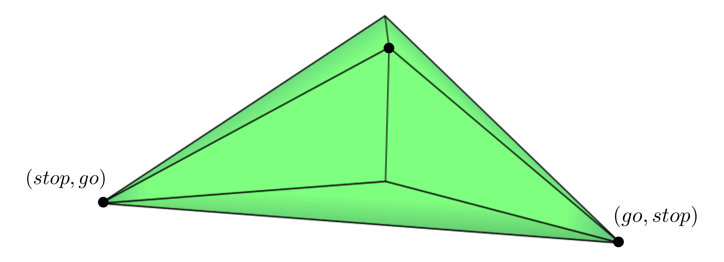
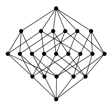
Figure 1. The correlated equilibrium polytope of the Traffic Lights example is a bipyramid where three of its vertices are Nash equilibria. Its $f$-vector is $(1,5,9,6,1)$ and its face lattice can be seen on the right.

We illustrate the concept of correlated equilibrium in an example: Two cars meet at a crossing. Both drivers would like to continue to drive, but, even more importantly, would also like to avoid a car crash. Thus, each of the drivers prefers not to drive in case the other chooses to drive. We make the assumptions that both drivers are unable to communicate with each other. This is a classic game in game theory known as Chicken game or Hawk-Dove game, and we formalize this in Examples 2.1, 2.3, 2.6 and 5.1. However, this situation changes drastically if there is a traffic light installed at this crossing. We can view the traffic light as a neutral exterior party, that gives a recommendation to each player in showing green or red lights; here we assume that each driver only knows their own given recommendation. If a fixed driver is given such a recommendation (for example a red light), the driver now ponders about deviating from this recommendation in benefit of their own (selfish) good, assuming that the other player adheres to their own given recommendation. If both drivers decide not to deviate from the recommendation given by the traffic lights, a correlated equilibrium is achieved.
To our knowledge, there are no articles concerning the combinatorics of correlated equilibrium polytopes in the language of convex geometry up to this date, despite the fact that the concept of correlated equilibria is a topic of extensive research in economics and game theory. In this article we study this class of polytopes from combinatorial perspective. In general, the correlated equilibrium polytope can exhibit a great variety of distinct combinatorial structures. This is not surprising as it is proven that any convex polytope can be realized as the correlated equilibrium payoffs of an $n$-player game [LSV11]. Even classifying necessary conditions under which the correlated equilibrium polytope is of maximal dimension is highly nontrivial [Vio03]. For this purpose, we introduce the region of full-dimensionality, a set that classifies under which conditions the correlated equilibrium polytope has maximal dimension.

Theorem 4.2.

The region of full-dimensionality is a semialgebraic set and can be explicitly described.

The full description of this semialgebraic set can be found on Theorem 4.2. We continue the study of the combinatorial structure of correlated equilibrium polytopes by introducing a linear space called the the correlated equilibrium space, and consider an oriented matroid strata inside this space. This is a stratification of the linear space, in which regions give rise to the different combinatorial types of correlated equilibrium polytopes. We study the algebraic boundary of the strata for $(2\times n)$-games, which turns out to be generated by binomials corresponding to $(2\times 2)$-minors of a certain matrix (Theorem 5.8). These investigations yield novel insights into the possible combinatorial types of $(2\times 3)$-games.

Theorem 5.9.

Let $G$ be a $(2\times 3)$-game and $P_{G}$ be the associated correlated equilibrium polytope. Then one of the following holds:

• $P_{G}$ is a point,

• $P_{G}$ is of maximal dimensional $5$ and of a unique combinatorial type,

• There exists a $(2\times 2)$-game $G^{\prime}$ such that $P_{G^{\prime}}$ has maximal dimensional $3$ is and combinatorially equivalent to $P_{G}$.

Supported by the above theorem and our computations [MR22] for $(2\times n)$-games $G$ (where $n\leq 5$), we conjecture that if $P_{G}$ is not of maximal dimension, then there exists a smaller $(2\times k)$-game $G^{\prime}$ with $k<n$ such that $P_{G^{\prime}}$ is a full-dimensional polytope and $P_{G}$ is combinatorially equivalent to $P_{G^{\prime}}$ (5.1).

Overview

We first provide a short introduction for the necessary concepts from game theory in Section 2, including correlated equilibria and Nash equilibria. In Section 3 we describe the correlated equilibrium cone, a convex polyhedral cone which captures the geometry of the correlated equilibrium polytope, and describe the correlated equilibrium space. We study the region of full-dimensionality in Section 4. Finally, we consider the possible combinatorial types through the oriented matroid strata in Section 5. All results are illustrated with examples for games of types $(2\times 2),\ (2\times 3)$ and, whenever possible, games of type $(2\times 2\times 2)$. All referenced code and a detailed study of some examples with visualizations can be found on MathRepo [MR22]:

https://mathrepo.mis.mpg.de/correlated-equilibrium

Acknowledgements

The authors would like to thank Rainer Sinn and Bernd Sturmfels for several helpful discussions.

2. The Correlated Equilibrium Polytope

Let $n$ be the number of players in a normal-form game. Each player $i\in[n]$ has a fixed set of pure strategies $s^{(i)}_{1},\dots s^{(i)}_{d_{i}},d_{i}\in\mathbb{N}$. It is practical to think of each strategy as a single move that a player can play, and all players perform their single move simultaneously. Afterwards, the game is over, so the choices of the possible moves can be seen as outcome of the game. A pure joint strategy is a tuple $s_{j_{1}\dots j_{n}}=(s^{(1)}_{j_{1}},\dots,s^{(n)}_{j_{n}})$ of strategies, where each player $i\in[n]$ chooses to play a fixed strategy $s^{(i)}_{j_{i}}$ with $j_{i}\in[d_{i}],i\in[n]$. The payoff $X^{(i)}_{j_{1}\dots j_{n}}\in\mathbb{R}$ of player $i$ at $s_{j_{1}\dots j_{n}}$ is the quantity of how beneficial player $i$ values the combination $(s^{(1)}_{j_{1}},\dots,s^{(n)}_{j_{n}})$ of strategies as outcome of the game. A mixed strategy of a single player $i$ is an action with probability $p^{(i)}=(p^{(i)}_{j_{1}},\dots,p^{(i)}_{j_{d_{i}}})$, i.e. $p^{(i)}_{j_{1}},\dots,p^{(i)}_{j_{d_{i}}}\geq 0$ and $\sum_{k=1}^{d_{i}}p^{(i)}_{j_{k}}=1$. We can view this geometrically as a point in the $(d_{i}-1)$-dimensional probability simplex $\Delta_{d_{i}-1}$.

Formally, a $(d_{1}\times\dots\times d_{n})$-game in normal form is a tuple $G=(n,S,X)$, where $S=\leavevmode\nobreak\ (S^{(1)},\dots,S^{(n)})$ is the collection of strategies $S^{(i)}=(s^{(i)}_{1},\dots,s^{(i)}_{d_{i}})$ of all players, and $X=\leavevmode\nobreak\ (X^{(1)},\dots,X^{(n)})$ is the collection of all $(d_{1}\times\cdots\times d_{n})$-payoff tensors. In particular, if $n=2$, then each $X^{(i)}$ is a $(d_{1}\times d_{2})$-matrix and called the payoff matrix of player $i$.

Example 2.1 (Traffic Lights).

Recall the example from the introduction, in which two cars meet at a crossing and would like to avoid a car crash. Formally, each player $i\in[2]$ has the strategies $s^{(i)}_{1}=$ “go” and $s^{(i)}_{2}=$ “stop”. The bimatrix below shows the payoffs of both players simultaneously, where each entry is a tuple $(X^{(1)}_{j_{1}j_{2}},X^{(2)}_{j_{1}j_{2}})$ of the payoff of each player for the tuple of strategies $(s^{(1)}_{j_{1}},s^{(2)}_{j_{2}}),j_{1},j_{2}\in[2]$ as the expected outcome of the game.

		Player $2$
		go	stop
Player $1$	go	$(-99,-99)$	$(1,0)$
	stop	$(0,1)$	$(0,0)$

We may interpret the given payoffs such that each of the players prefers to go (with payoff $X^{(1)}_{12}=X^{(2)}_{21}=1$), if the other driver stops. However, both drivers choosing to drive is the worst possible outcome for each of the players individually (with payoff $X^{(i)}_{11}=-99$ for both players). Since there is no interaction between the players, and the payoffs of a car crash are very negative, the players are very likely not to risk a move, although this is not optimal for either of these players ($X^{(i)}_{22}=0$ for both players). This is the motivation for introducing the concept of correlated equilibrium, in which the assumptions allow a dependence of the moves of the players by the suggestion of an external party e.g. a traffic light. We continue with this in Examples 2.3 and 2.6.

We now allow a third, independent party to influence the game from the outside. Let $\tilde{S}=\{s_{j_{1}\dots j_{n}}\mid j_{i}\in[d_{i}],i\in[n]\}$ be the set of all pure joint strategies of the game. The external party draws such a pure joint strategy with probability $p_{j_{1}\dots j_{n}}\geq 0$, called a mixed joint strategy. Such a joint probability distribution is a vector (or a tensor) $p=(p_{j_{1}\dots j_{n}}\mid j_{i}\in[d_{i}],i\in[n])$, such that $\sum_{j_{1}=1}^{d_{1}}\cdots\sum_{j_{n}=1}^{d_{n}}p_{j_{1}\dots j_{n}}=1$. The set of all joint probability distributions is the probability simplex $\Delta_{d_{1}\cdots d_{n}-1}$.

Definition 2.2 (Correlated Equilibrium).

Let $G$ be a game with payoffs $X=(X^{(1)},\dots,X^{(n)})$. A point $p\in\Delta_{d_{1}\cdots d_{n}-1}$ is a correlated equilibrium if and only if

(2.1) $$\sum_{j_{1}=1}^{d_{1}}\cdots\widehat{\sum_{j_{i}=1}^{d_{i}}}\cdots\sum_{j_{n}=1}^{d_{n}}\left(X^{(i)}_{j_{1}\cdots j_{i-1}kj_{i+1}\cdots j_{n}}-X^{(i)}_{j_{1}\cdots j_{i-1}lj_{i+1}\cdots,j_{n}}\right)p_{j_{1}\cdots j_{i-1}kj_{i+1}\cdots j_{n}}\geq 0.$$

for all $k,l\in[d_{i}]$, and for all $i\in[n]$. The linear inequalities in (2.1) together with the linear constrains

$$p_{j_{1}\dots j_{n}}\geq 0\text{ for }j_{i}\in[d_{i}],i\in[n],\text{ and }\sum_{j_{1}=1}^{d_{1}}\cdots\sum_{j_{n}=1}^{d_{n}}p_{j_{1}\dots j_{n}}=1$$

define the set of all correlated equilibria of the game. The set of all such equilibria is the correlated equilibrium polytope $P_{G}$ of the game $G$.

The ambient space of the polytope $P_{G}$ has dimension $d_{1}\cdots d_{n}$. By definition, the maximal dimension that $P_{G}$ can achieve is $d_{1}\cdots d_{n}-1$. In the literature, in this case, $P_{G}$ is often called full-dimensional. To avoid confusion with conventions in convex geometry, we refer to $P_{G}$ as having maximal dimension.

Example 2.3 (Traffic Lights).

We continue with Example 2.1. Here, the third party is given by a traffic light at the crossing. The traffic light gives the recommendation “go” to a driver if turns green, and “stop” if it turns red. The traffic light draws randomly from one of the combinations of strategies. Let $p_{j_{1}j_{2}}$ be the probability with which the traffic light draws the pure joint strategy $s_{j_{1}j_{2}}$. The point $p=(p_{11},p_{12},p_{21},p_{22})$ is a correlated equilibrium if and only if $p_{j_{1}j_{2}}\geq 0,\ p_{11}+p_{12}+p_{21}+p_{22}=1$ and

$$(X^{(1)}_{\text{22}}-X^{(1)}_{\text{12}})p_{\text{22}}+(X^{(1)}_{\text{21}}-X^{(1)}_{\text{11}})p_{\text{21}}\geq 0,\qquad(X^{(1)}_{\text{12}}-X^{(1)}_{\text{22}})p_{\text{12}}+(X^{(1)}_{\text{11}}-X^{(1)}_{\text{21}})p_{\text{11}}\geq 0,$$

$$(X^{(2)}_{\text{22}}-X^{(2)}_{\text{21}})p_{\text{22}}+(X^{(2)}_{\text{12}}-X^{(2)}_{\text{11}})p_{\text{12}}\geq 0,\qquad(X^{(2)}_{\text{21}}-X^{(2)}_{\text{22}})p_{\text{21}}+(X^{(2)}_{\text{11}}-X^{(2)}_{\text{12}})p_{\text{11}}\geq 0.$$

With the payoffs as given in the bimatrix in Example 2.1 these inequalities evaluate to

$$-p_{\text{22}}+99p_{\text{21}}\geq 0, p_{\text{12}}-99p_{\text{11}}\geq 0,$$

$$-p_{\text{22}}+99p_{\text{12}}\geq 0 p_{\text{21}}-99p_{\text{11}}\geq 0.$$

The correlated equilibrium polytope, i.e. the points $p$ that satisfy these inequalities, has $5$ vertices with coordinates $(0,0,1,0),$ $(0,1,0,0),$ $(\tfrac{1}{10000},\tfrac{99}{10000},\tfrac{99}{10000},\tfrac{9801}{10000}),$ $(0,\tfrac{1}{101},\tfrac{1}{101},\tfrac{99}{101}),$ $(\tfrac{1}{199},\tfrac{99}{199},\tfrac{99}{199},0)$. This polytope is depicted in Figure 2.

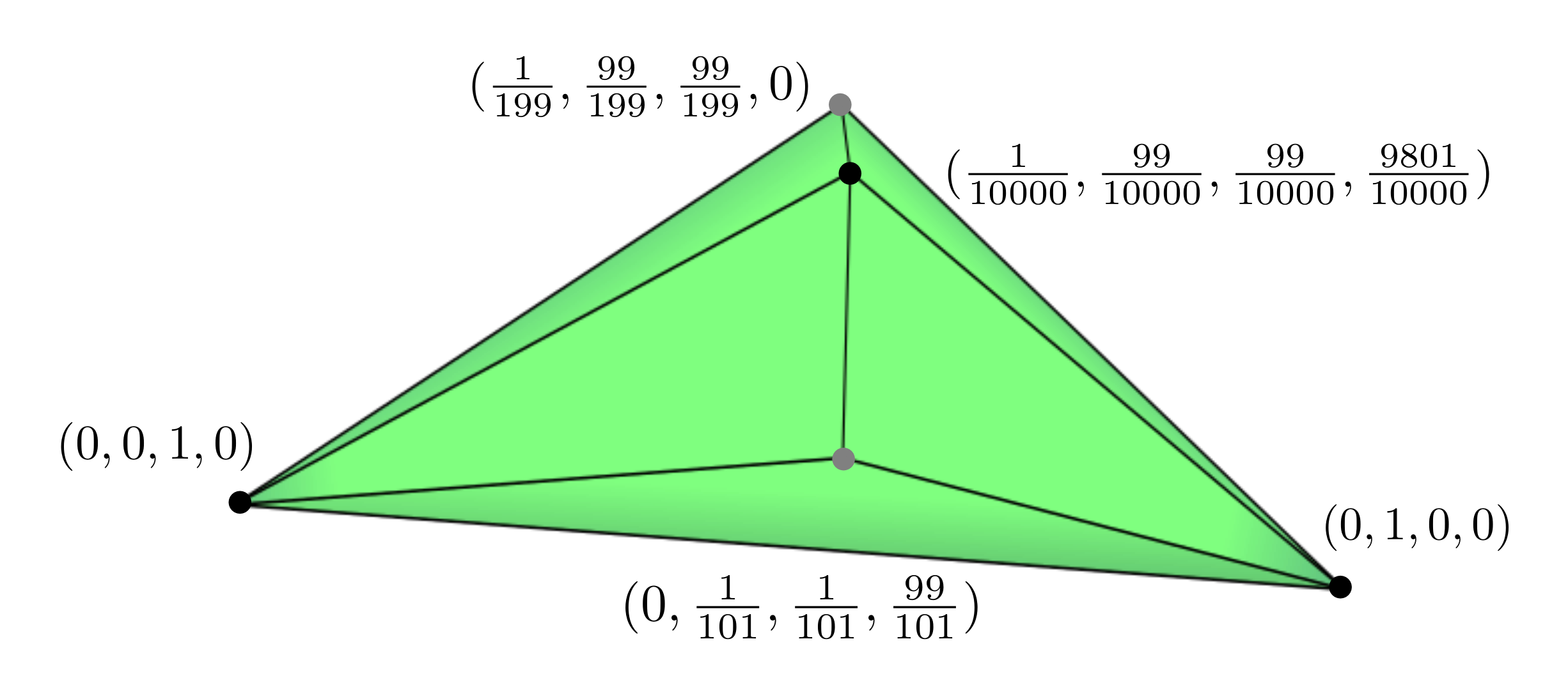
Figure 2. The vertices of the correlated equilibrium polytope for the Traffic Lights example (Example 2.3)

The next proposition shows that two affinely dependent games define the same correlated equilibrium polytope.

Proposition 2.4.

Any affine linear transformation of the payoff tensors $X^{(i)}$ with positive scalars leaves the polytope $P_{G}$ invariant. More precisely, let $G=(n,S,X)$ be a game. For each $i\in[n]$, fix $t_{i}\in\mathbb{R},\ \lambda_{i}\in\mathbb{R}_{>0}$ and let $\tilde{X}^{(i)}_{j_{1}\dots j_{n}}=\lambda_{i}X^{(i)}_{j_{1}\dots j_{n}}+t_{i}$ for all $j_{k}\in[d_{k}],k\in[n]$. Then for the game $\tilde{G}=(n,\tilde{X},S)$ with $\tilde{X}=(\tilde{X}^{(1)},\dots,\tilde{X}^{(n)})$ it holds that $P_{G}=P_{\tilde{G}}$.

Proof.

For each player $i\in[n]$ let $X^{(i)}$ be their payoff tensor, fix $t_{i}\in\mathbb{R},\ \lambda_{i}\in\mathbb{R}_{>0}$, and consider the affine transformation $\tilde{X}^{(i)}_{j_{1}\dots j_{n}}=\lambda_{i}X^{(i)}_{j_{1}\dots j_{n}}+t_{i}$. Then

$$\sum_{j_{1}=1}^{d_{1}}\dots\widehat{\sum_{j_{i}=1}^{d_{i}}}\dots\sum_{j_{n}=1}^{d_{n}}\left(\tilde{X}^{(i)}_{j_{1}\dots j_{i-1}kj_{i+1}\dots j_{n}}-\tilde{X}^{(i)}_{j_{1}\ldots j_{i-1}lj_{i+1}\dots j_{n}}\right)p_{j_{1}\dots j_{i-1}kj_{i+1}\dots j_{n}}$$

$$= \sum_{j_{1}=1}^{d_{1}}\dots\widehat{\sum_{j_{i}=1}^{d_{i}}}\dots\sum_{j_{n}=1}^{d_{n}}\left(\lambda_{i}X^{(i)}_{j_{1}\dots j_{i-1}kj_{i+1}\dots j_{n}}+t_{i}-\lambda_{i}X^{(i)}_{j_{1}\dots j_{i-1}lj_{i+1}\dots j_{n}}-t_{i}\right)p_{j_{1}\dots j_{i-1}kj_{i+1}\dots j_{n}}$$

$$= \lambda_{i}\sum_{j_{1}=1}^{d_{1}}\dots\widehat{\sum_{j_{i}=1}^{d_{i}}}\dots\sum_{j_{n}=1}^{d_{n}}\left(X^{(i)}_{j_{1}\dots j_{i-1}kj_{i+1}\dots j_{n}}-X^{(i)}_{j_{1}\dots j_{i-1}lj_{i+1}\dots j_{n}}\right)p_{j_{1}\dots j_{i-1}kj_{i+1}\dots j_{n}}\geq 0.$$

Since $\lambda_{i}>0$, this is equivalent to (2.1) being nonnegative. ∎

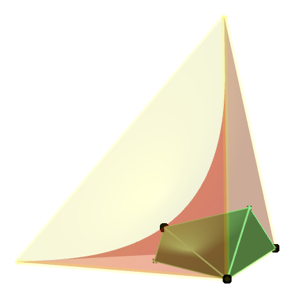
Figure 3. A $3$-dimensional correlated equilibrium polytope (green) inside the probability simplex $\Delta_{3}$ (yellow) for a $(2\times 2)$-game. Its Nash equilibria (black) are the intersection with the Segre variety (red). This picture applies to the Traffic Lights example (Examples 2.1, 2.3 and 2.6) as well as the Hawk-Dove game (Example 5.1).

Definition 2.5 (Nash Equilibrium).

Let $G$ be a game. A Nash equilibrium of $G$ is a point $p\in P_{G}$ that is a tensor of rank one. More specifically, the set of Nash equilibria are those points in $P_{G}$ that are also contained in the image of the product map

$$\varphi:\Delta_{d_{1}-1}\times\cdots\times\Delta_{d_{n}-1} \rightarrow\Delta_{d_{1}\cdots d_{n}-1}$$

$$(p^{(1)},\dots,p^{(n)}) \mapsto p^{(1)}_{j_{1}}\cdot\ldots\cdot p^{(n)}_{j_{n}}$$

The image of this map is the Segre variety inside $\Delta_{d_{1}\cdots d_{n}-1}$.

Figure 3 shows a $3$-dimensional correlated equilibrium polytope of a $(2\times 2)$-game together with the Segre variety inside the simplex $\Delta_{3}$. We illustrate this in more details in the following example.

Example 2.6 (Traffic Lights).

We continue with the Traffic Lights example from Examples 2.1 and 2.3. The Nash equilibria of this game occur as vertices of the correlated equilibrium polytope $P_{G}$. More precisely, they occur as the images of the points $(p^{(1)},p^{(2)})\in\Delta_{2}\times\Delta_{2}$ with coordinates $((1,0),(0,1)),\ ((0,1),(1,0))$ and $((\tfrac{1}{100},\tfrac{99}{100}),((\tfrac{1}{100},\tfrac{99}{100}))$ under the product map $\varphi$ from Definition 2.5, which correspond to the three black vertices in Figure 2. With indexing $p=(p_{11},p_{12},p_{21},p_{22})$ the images of the first two points are $p=(0,1,0,0)$ and $(0,0,1,0)$. These are the probability distributions which correspond to the pure joint strategies in which one of the players drives, while the other one stops. The point $p=(\tfrac{1}{10000},\tfrac{99}{10000},\tfrac{99}{10000},\tfrac{9801}{10000})$ is a probability distribution in which it is most likely that both players stop.

By Definition 2.5, the set of Nash equilibria is a subset of the correlated equilibrium polytope. However, characterizing Nash equilibria is computationally difficult. Therefore, it is of interest to understand where the Nash equilibria lie relative to the correlated equilibrium polytope [PR05]. A game $G$ is called non-trivial if $X^{(i)}_{j_{1}\ldots j_{i-1}kj_{i+1},\dots j_{n}}\neq X^{(i)}_{j_{1}\ldots j_{i-1}lj_{i+1},\ldots j_{n}}$ for some player $i\in[n]$ and $k,l\in[d_{i}]$ with $k\neq l$. The next result states that if $P_{G}$ is of maximal dimension, then any Nash equilibrium lies on a proper face of $P_{G}$.

Proposition 2.7 ([NCH04, Proposition 1]).

Let $G$ be a non-trivial game. Then the Nash equilibria lie on a face of the correlated equilibrium polytope $P_{G}$ of dimension at most $d_{1}\cdots d_{n}-2$. In particular, if $P_{G}$ has maximal dimension $d_{1}\cdots d_{n}-1$, then the Nash equilibria lie on the relative boundary of $P_{G}$.

In order to locate the possible positions of Nash equilibria, it is thus helpful to understand the conditions under which $P_{G}$ is of maximal dimension. In Section 4 we study the region of full-dimensionality, which formalizes these conditions.

3. The Correlated Equilibrium Cone

The combinatorics of the correlated equilibrium polytope is completely determined by the cone given by the inequality constraints (2.1), intersected with the nonnegative orthant. The correlated equilibrium cone $C_{G}\subseteq\mathbb{R}^{d_{1}\cdots d_{n}}$ is the polyhedral cone defined by inequalities $p_{j_{1}\dots j_{n}}\geq 0$ and

(3.1) $$\sum_{j_{1}=1}^{d_{1}}\cdots\widehat{\sum_{j_{i}=1}^{d_{i}}}\cdots\sum_{j_{n}=1}^{d_{n}}\left(X^{(i)}_{j_{1}\cdots j_{i-1}kj_{i+1}\cdots j_{n}}-X^{(i)}_{j_{1}\cdots j_{i-1}lj_{i+1}\cdots j_{n}}\right)p_{j_{1}\cdots j_{i-1}kj_{i+1}\cdots j_{n}}\geq 0.$$

for all $k,l\in[d_{i}]$, and for all $i\in[n]$. For each player $i\in[n]$ this defines $d_{i}(d_{i}-1)$ nontrivial inequalities of type (3.1). The cone $C_{G}$ is a convex pointed polyhedral cone. The correlated equilibrium polytope $P_{G}$ is the intersection of the cone with the hyperplane where the sum of all coordinates equals $1$. Therefore, a facet of $P_{G}$ is in bijection with a facet of $C_{G}$, and a vertex of $P_{G}$ is in bijection with an extremal ray of $C_{G}$.

We make a substitution of the coefficients in (3.1). For each $i\in[n],j_{1}\in[d_{1}],\dots,j_{i-1}\in\leavevmode\nobreak\ [d_{i-1}]$, $k,l\in[d_{i}],\ j_{i+1}\in[d_{i+1}],\dots,j_{n}\in[d_{n}]$ we define

$$Y^{(i)}_{j_{1}\cdots\hat{j_{i}}\cdots j_{n}}(k,l)=X^{(i)}_{j_{1}\cdots j_{i-1}kj_{i+1}\cdots j_{n}}-X^{(i)}_{j_{1}\cdots j_{i-1}lj_{i+1}\cdots j_{n}}.$$

Note that $Y^{(i)}_{j_{1}\dots\hat{j_{i}}\dots j_{n}}(k,l)=-Y^{(i)}_{j_{1}\dots\hat{j_{i}}\dots j_{n}}(l,k)$. Thus, for each player $i\in[n]$ this defines $\binom{d_{i}}{2}\prod_{\begin{subarray}{c}k\in[n]\\ k\neq i\end{subarray}}d_{k}$ distinct variables, so in total this defines

$$M=\sum_{i=1}^{n}\binom{d_{i}}{2}\prod_{\begin{subarray}{c}k\in[n]\\ k\neq i\end{subarray}}d_{k}$$

many variables. Under this substitution, the above inequality becomes

(3.2) $$\sum_{j_{1}=1}^{d_{1}}\cdots\widehat{\sum_{j_{i}=1}^{d_{i}}}\cdots\sum_{j_{n}=1}^{d_{n}}Y^{(i)}_{j_{1}\cdots\hat{j_{i}}\cdots j_{n}}(k,l)\ p_{j_{1}\cdots j_{n}}\geq 0.$$

For fixed $i\in[n],k,l\in[d_{i}]$, let $U^{(i)}_{kl}\in\mathbb{R}^{d_{1}\cdots d_{n}}$ be the vector with entries

$$(U^{(i)}_{kl})_{j_{1}\dots j_{i}\dots j_{n}}=\begin{cases}Y^{(i)}_{j_{1}\dots\hat{j_{i}}\dots j_{n}}(k,l)&\text{if }j_{i}=k\text{ and }k<l\\[10.0pt] -Y^{(i)}_{j_{1}\dots\hat{j_{i}}\dots j_{n}}(k,l)&\text{if }j_{i}=k\text{ and }k>l\\[10.0pt] 0&\text{otherwise}\end{cases}$$

for each coordinate indexed by $j_{1}\in[d_{1}],\dots,j_{i}\in[d_{i}],\dots,j_{n}\in[d_{n}]$. Using the same indexing of coordinates for $p\in\mathbb{R}^{d_{1}\cdot\ldots\cdot d_{n}}$, the inequalities (3.2) can be expressed as the inner product $\langle U^{(i)}_{kl},p\rangle\geq 0$.

Example 3.1 ($(2\times 2)$-games).

Consider a $2$-player game with $d_{1}=d_{2}=2$. We fix the indexing $p=(p_{11},p_{12},p_{21},p_{22})$. Recall that the inequalities are

$$(X^{(1)}_{11}-X^{(1)}_{21})p_{11}+(X^{(1)}_{12}-X^{(1)}_{22})p_{12} =Y^{(1)}_{1}(1,2)\ p_{11}+Y^{(1)}_{2}(1,2)\ p_{12}\geq 0$$

$$(X^{(1)}_{21}-X^{(1)}_{11})p_{21}+(X^{(1)}_{22}-X^{(1)}_{12})p_{22} =-Y^{(1)}_{1}(1,2)\ p_{21}-Y^{(1)}_{2}(1,2)\ p_{22}\geq 0$$

$$(X^{(2)}_{21}-X^{(2)}_{22})p_{21}+(X^{(2)}_{11}-X^{(2)}_{12})p_{11} =Y^{(2)}_{2}(1,2)\ p_{21}+Y^{(2)}_{1}(1,2)\ p_{11}\geq 0$$

$$(X^{(2)}_{22}-X^{(2)}_{21})p_{22}+(X^{(2)}_{12}-X^{(2)}_{11})p_{12} =-Y^{(2)}_{2}(1,2)\ p_{22}-Y^{(2)}_{1}(1,2)\ p_{12}\geq 0.$$

The vectors $U^{(i)}_{kl}$ have entries in the $4$ unknowns $Y^{(1)}_{1}(1,2)\ ,Y^{(1)}_{2}(1,2)\ ,Y^{(2)}_{1}(1,2)\ ,Y^{(2)}_{2}(1,2)$. More specifically,

$$U^{(1)}_{12} =(Y^{(1)}_{1}(1,2)\ ,Y^{(1)}_{2}(1,2)\ ,0,0)$$

$$U^{(1)}_{21} =-(0,0,Y^{(1)}_{1}(1,2)\ ,Y^{(1)}_{2}(1,2))$$

$$U^{(2)}_{12} =(Y^{(2)}_{1}(1,2)\ ,0,Y^{(2)}_{2}(1,2)\ ,0)$$

$$U^{(2)}_{21} =-(0,Y^{(2)}_{1}(1,2)\ ,0,Y^{(2)}_{2}(1,2)).$$

The cone $C_{G}$ is defined by the inequalities $\langle U^{(i)}_{kl},p\rangle\geq 0$ for $i\in[2]$, and $k,l\in[2],k\neq l$, and the inequalities $\langle e_{i},p\rangle\geq 0$, where $e_{i}$ denote the standard basis vectors of $\mathbb{R}^{4}$.

Recall that the number of variables defined above is $M=\sum_{i=1}^{n}\binom{d_{i}}{2}\prod_{\begin{subarray}{c}k\in[n]\\ k\neq i\end{subarray}}d_{k}$. The ambient dimension of the correlated equilibrium polytope and cone is $D=\prod_{i=1}^{n}d_{i}$, and the number of linear inequalities of the form (3.2) is $N=\sum_{i=1}^{n}d_{i}(d_{i}-1)$. Let $U=U(Y)\in\mathbb{R}^{N\times D}$ be the matrix with rows $U^{(i)}_{kl}$ for $i\in[n],k,l\in[d_{i}],k\neq l$, and let $A(Y)\in\mathbb{R}^{(D+N)\times D}$ be the block matrix

$$A(Y)=\begin{pmatrix}U\\ Id_{D}\end{pmatrix}.$$

By (3.2), the cone $C_{G}=C(Y)$ is given by

$$C(Y)=\{p\in\mathbb{R}^{D}\mid A(Y)p\geq 0\}.$$

The matrix $A(Y)$ has full rank $D$, and so $C(Y)$ is a pointed cone.

For $(d_{1}\times\dots\times d_{n})$-games, where $d_{i}\geq 3$ for some $i\in[n]$, we have additional relations

(3.3) $$Y^{(i)}_{j_{1}\cdots\hat{j_{i}}\cdots j_{n}}(k,l)+Y^{(i)}_{j_{1}\cdots\hat{j_{i}}\cdots j_{n}}(l,t)=Y^{(i)}_{j_{1}\cdots\hat{j_{i}}\cdots j_{n}}(k,t)$$

for $j_{1}\in[d_{1}],\dots,j_{i-1}\in[d_{i-1}],\ k,l,t\in[d_{i}],\ j_{i+1}\in[d_{i+1}],\dots,j_{n}\in[d_{n}]$. A vector $Y\in\mathbb{R}^{M}$ corresponds to a certain game $G$ if and only if these relations hold. Geometrically, these relations define a linear space inside $\mathbb{R}^{M}$. We thus make the following definition.

Definition 3.2.

The correlated equilibrium space $\mathcal{S}\subseteq\mathbb{R}^{M}$ of $(d_{1}\times\dots\times d_{n})$-games is the linear space defined by the equations (3.3), where $i\in[n]$ ranges over all players with at least $3$ strategies $d_{i}\geq 3$. If all players have at most $2$ strategies, then no such relation among the variables holds, and the correlated equilibrium space is the entire ambient space $\mathcal{S}=\mathbb{R}^{M}$.

Example 3.3 ($\mathcal{S}$ for $(2\times 3)$-games).

In a $(2\times 3)$-game, there are six variables

$$Y^{(1)}_{1}(1,2)=X^{(1)}_{11}-X^{(1)}_{21},\qquad Y^{(1)}_{2}(1,2)=X^{(1)}_{12}-X^{(1)}_{22},\qquad Y^{(1)}_{3}(1,2)=X^{(1)}_{13}-X^{(1)}_{23},$$

$$Y^{(2)}_{1}(1,2)=X^{(2)}_{11}-X^{(2)}_{12},\qquad Y^{(2)}_{1}(1,3)=X^{(2)}_{11}-X^{(2)}_{13},\qquad Y^{(2)}_{1}(2,3)=X^{(2)}_{12}-X^{(2)}_{13},$$

$$Y^{(2)}_{2}(1,2)=X^{(2)}_{21}-X^{(2)}_{22},\qquad Y^{(2)}_{2}(1,3)=X^{(2)}_{21}-X^{(2)}_{23},\qquad Y^{(2)}_{2}(2,3)=X^{(2)}_{22}-X^{(2)}_{23}.$$

The relations among these variables are

$$Y^{(2)}_{1}(1,2)+Y^{(2)}_{1}(2,3)=Y^{(2)}_{1}(1,3),\qquad Y^{(2)}_{2}(1,2)+Y^{(2)}_{2}(2,3)=Y^{(2)}_{2}(1,3).$$

These relations cut out the correlated equilibrium space $\mathcal{S}$ for $(2\times 3)$-games. For any game $(2\times 3)$-games $G$ the correlated equilibrium polytope is nonempty, a so point $Y\in\mathbb{R}^{6}$ defines a correlated equilibrium cone if and only if it satisfies the above relations.

Remark 3.4.

In the following sections we will classify correlated equilibrium polytopes and cones with respect to the variables $Y$ instead of the payoff tensors $X$. We note that this is not a significant restriction, as this is a linear change of coordinates and thus does not change the geometry of the objects described in what follows, provided one restricts to the correlated equilibrium space $\mathcal{S}$.

4. The Region of Full-Dimensionality

In this section we introduce the region of full-dimensionality for a type of games. For fixed $d_{i}\in\leavevmode\nobreak\ \mathbb{N},i\in[n]$, this region classifies for which $(d_{1}\times\dots\times d_{n})$-games the polytope $P_{G}$ is of maximal dimension $D-1=d_{1}\cdots d_{n}-1$. Recall from Proposition 2.7 that the dimension of $P_{G}$ may determine the possible positions of Nash equilibria. The connections between full-dimensionality and elementary games are discussed in [Vio03]. In general, it is not understood under which conditions $P_{G}$ has maximal dimension (i.e. $G$ is a full game), though there are some partial results on forbidden dimensions [Vio10, Proposition 7].

Let $Y\in\mathcal{S}\subseteq\mathbb{R}^{M}$ be a vector of indeterminates, as described in Section 3. We consider $A=A(Y)$ as a matrix with indeterminates, where each choice of $Y\in\mathbb{R}^{M}$ uniquely defines a correlated equilibrium cone

$$C(Y)=\{p\in\mathbb{R}^{N}\mid A(Y)p\geq 0\}.$$

Recall that the correlated equilibrium polytope $P_{G}(Y)$ is of maximal dimension if and only if $C(Y)$ is full-dimensional. Thus, we are interested in the region of full-dimensionality

$$\mathcal{D}=\{Y\in\mathcal{S}\subseteq\mathbb{R}^{M}\mid\dim(C(Y))=D\}.$$

Definition 4.1.

A semialgebraic set is a subset of $\mathbb{R}^{M}$ defined by a boolean combination of finitely many polynomial inequalities.

Theorem 4.2.

The region $\mathcal{D}$ of full-dimensionality is the semialgebraic set

$$\pi_{Y}(\{(x,Y)\in\mathbb{R}^{D+M}\mid A(Y)x>0\})\cap\mathcal{S}$$

where $\pi_{Y}$ is the coordinate projection onto the last $M$ coordinates.

Proof.

The cone $C(Y)$ is full-dimensional if and only if it has nonempty interior, i.e. if there exists some $p\in\mathbb{R}^{D}$ such that $A(Y)p>0$. Let $x=(x_{j_{1}\cdots j_{n}}\mid i\in[n],j_{i}\in[d_{i}])$ be a vector of $D$ indeterminates. Consider the set

$$\{(x,Y)\in\mathbb{R}^{D+M}\mid A(Y)x>0\}.$$

The expression $A(Y)x$ defines a $(D+N)$-dimensional vector, where each coordinate is a polynomial in variables $x$ and $Y$. Hence, the set $\{(x,Y)\in\mathbb{R}^{D+M}\mid A(Y)x>0\}$ is defined by $D+N$ polynomial inequalities, and is thus a (basic) semialgebraic set. The region $\mathcal{D}$ of full-dimensionality is the intersection of the correlated equilibrium space $\mathcal{S}$ with a coordinate projection of this set, which can be obtained by projecting away the $x$-coordinates. The Tarski–Seidenberg theorem implies that the coordinate projection is semialgebraic, and hence $\mathcal{D}$ is a semialgebraic set. ∎

Example 4.3 ($\mathcal{D}$ for $(2\times 2)$-games).

Consider a $(2\times 2)$-game. In this case, the ambient dimension of the correlated equilibrium polytope is $D=4$, the number of incentive constraints is $N=4$ (so the number of inequalities that define the polytope is $D+N=8$) and the ambient dimension of $\mathcal{D}\subseteq\mathcal{S}=\mathbb{R}^{M}$ is $M=4$. The different combinatorial types in this case have been fully classified in [CA03]. Here, $\mathcal{D}\subseteq\mathbb{R}^{4}$ is the union of two open orthants:

$$a)\ Y^{(1)}_{1}(1,2)>0,\ Y^{(1)}_{2}(1,2)<0,\ Y^{(2)}_{1}(1,2)>0,\ Y^{(2)}_{2}(1,2)<0$$

$$b)\ Y^{(1)}_{1}(1,2)<0,\ Y^{(1)}_{2}(1,2)>0,\ Y^{(2)}_{1}(1,2)<0,\ Y^{(2)}_{2}(1,2)>0$$

The file dimensions2x2.nb in [MR22] contains Mathematica code [Wol22] which also computes these inequalities.

Example 4.4 ($\mathcal{D}$ for $(2\times 3)$-games).

The coordinate projection of the set $\{(x,Y)\in\mathbb{R}^{D+M}\mid A(Y)x>0\}$ onto $\mathbb{R}^{M}$ is the union of basic semialgebraic sets, where each piece is the intersection of an orthant with a binomial inequality. One of the pieces is

$$Y^{(1)}_{1}(1,2)>0,\ Y^{(1)}_{2}(1,2)>0,\ Y^{(1)}_{3}(1,2)<0,$$

$$Y^{(2)}_{1}(1,2)<0,\ Y^{(2)}_{1}(1,3)<0,\ Y^{(2)}_{1}(2,3)>0,\ Y^{(2)}_{2}(1,2)>0,\ Y^{(2)}_{2}(1,3)>0,\ Y^{(2)}_{2}(2,3)<0,$$

$$Y^{(2)}_{2}(1,3)\ Y^{(2)}_{1}(2,3)<Y^{(2)}_{1}(1,3)\ Y^{(2)}_{2}(2,3).$$

The region $\mathcal{D}$ of full-dimensionality for $(2\times 3)$-games consists of the intersection of the above mentioned pieces with the correlated equilibrium space $\mathcal{S}$. The Mathematica file dimensions2x3.nb in [MR22] contains our code for computing all of the components of this semialgebraic set. We note that the orthants appearing in $\mathcal{D}$ seem highly structured.

Remark 4.5.

The structured behaviour of the regions of full-dimensionality that we see in $(2\times 3)$-games arises more generally for arbitrary $(2\times n)$-games. Exploiting the structure of the matrix $A(Y)$, the region $\mathcal{D}$ of full-dimensionality for $(2\times n)$-games cannot satisfy any of the following conditions:

• $Y_{k}^{(1)}(1,2)>0$, for all $k\in[n]$.

• $Y_{k}^{(1)}(1,2)<0$, for all $k\in[n]$.

• $Y_{1}^{(2)}(k,n)>0$ and $Y_{2}^{(2)}(k,n)>0$, for all $k\in[n]$

• $Y_{1}^{(2)}(k,n)<0$ and $Y_{2}^{(2)}(k,n)<0$, for all $k\in[n]$.
  

While this approach could theoretically be used to obtain inequalities for larger games, this is extremely difficult in practice since the required algebraic methods do not scale well as the number of variables involved increases. For example, we were unable to carry out this computation for $(2\times 2\times 2)$-games since we must compute the coordinate projection of a semialgebraic set which lives in $D+M=20$-dimensional space.

5. Combinatorial Types of Correlated Equilibrium Polytopes

In this section, we consider how to systematically classify combinatorial types of polytopes arising as a correlated equilibrium polytope. The face lattice of a polytope $P$ is the poset of all the faces of $P$, partially ordered by inclusion. Two polytopes have the same combinatorial type if there exists an isomorphism between their face lattices.
First, we present a systematic approach for classifying the possible combinatorial types for arbitrary games by describing the oriented matroid strata. Even for small examples the explicit computation of the oriented matroid strata is beyond current scope, but we introduce algebraic methods for understanding the oriented matroid strata via its algebraic boundary. We use this technique to completely classify the combinatorial types of $P_{G}$ for $(2\times 3)$-games (Theorem 5.9). We then show that for all $(2\times n)$-games the irreducible components of the algebraic boundary of the oriented matroid strata are coordinate hyperplanes and $(2\times 2)$-minors of the matrix $A(Y)$ (Theorem 5.8).

Example 5.1 (Hawk-Dove game).

This game models a scenario of a competition for a shared resource. Both players can choose between conflict (hawk) or conciliation (dove) and is a generalization of the Traffic Lights example (Examples 2.1, 2.3 and 2.6). The inequalities for general $(2\times 2)$-games are given in Example 3.1. In the Hawk-Dove game, each of the two players has two strategies $s^{(i)}_{1}$=“hawk” or $s^{(i)}_{2}$=“dove”.

		Player $2$
		Hawk	Dove
Player $1$	Hawk	$\left(\frac{V-C}{2},\frac{V-C}{2}\right)$	$(V,0)$
	Dove	$(0,V)$	$\left(\frac{V}{2},\frac{V}{2}\right)$

In this bimatrix game, $V$ represents the value of the resource and $C$ represents the cost of the escalated fight. It is mostly assumed that $C>V>0$. The correlated equilibria polytope $P_{G}$ is full-dimensional with $5$ vertices and $6$ facets. In the case $V\geq C>0$, the game becomes an example for Prisoner’s Dilemma, in which case $P_{G}$ is a single point.

As seen in the previous example, for fixed $d_{1},\dots,d_{n}\in\mathbb{N}$, different choices of the payoffs for the players in a $(d_{1}\times\dots\times d_{n})$-game can result in different combinatorial types of correlated equilibria. We would thus like to classify the regions of the correlated equilibrium space $\mathcal{S}\subseteq\mathbb{R}^{M}$ such that

$$\{Y\in\mathcal{S}\mid C(Y)\text{ has a fixed combinatorial type}\}.$$

We now explain how the combinatorial type of $C(Y)$ is completely determined by the underlying oriented matroid defined by the matrix $A(Y)$. The combinatorial type of $C(Y)$ is the incidence structure of rays and facets of $C(Y)$. Equivalently, we can classify the incidence structure of facets and rays of the dual cone $C(Y)^{\ast}$. The dual of the cone $C(Y)$ is defined as

$$C(Y)^{*}=\{q\in\mathbb{R}^{d_{1}\cdots d_{n}}\mid\langle p,q\rangle\geq 0,\ \forall p\in C(Y)\}.$$

By definition, the (inner) facet normals of $C(Y)$ are generators of extremal rays of $C(Y)^{*}$ and vice versa. Let $h\in[D+N]$ and $A_{h}(Y)$ be a row of $A(Y)$. Seen as a linear functional, this row uniquely selects a face

$$F_{h}=\{p\in C(Y)\mid\langle A_{h}(Y),p\rangle=0\}.$$

Note that this is not necessarily a facet of $C(Y)$, but all facets of $C(Y)$ arise in this way. For the dual cone $C(Y)^{\ast}$ this implies that $r_{h}=A_{h}(Y)\mathbb{R}_{\geq 0}$ is an extremal ray of $C(Y)^{*}$ if and only if $F_{h}$ is a facet of $C$. If $C(Y)$ is not full-dimensional, then there is some $h\in[D+N]$ such that $F_{h}=C(Y)$. The set of all such vectors span the lineality space

$$\mathcal{L}=C(Y)^{*}\cap(-C(Y)^{*})=\text{span}(\{A_{h}\mid F_{h}=C(Y)\})$$

of $C^{*}(Y)$. In this case, extremal rays of $C(Y)^{*}$ are to be considered in $C(Y)^{*}/\mathcal{L}$.

We want to understand the incidence structure of extremal rays and facets of $C(Y)$. Each such ray of $C(Y)$ is contained in at least $D-1$ facets. Thus, we seek to understand which subsets of $D-1$ faces $F_{h}$ of $C(Y)$ intersect in a single point. Equivalently, we want to understand which subsets of $D-1$ rays $r_{h}$ of $C^{*}(Y)$ are contained in a common face. Let $H\subseteq[D+N]$ such that $|H|=D-1$, and denote by $A_{H}(Y)$ the submatrix of $A(Y)$ with rows indexed by $H$. If $\{r_{h}\mid h\in H\}$ lie on a common face, then these rays all lie on the hyperplane given by the rowspan of $A_{H}(Y)$. Additionally, let $h^{\prime}\in[D+N]\setminus H$. Then all $r_{h^{\prime}}$ lie on the same side of the hyperplane. This implies that the sign of $\det(A_{H\cup h^{\prime}})$ is uniquely determined for all $h^{\prime}\in[D+N]\setminus H$. The collection of all regions $\mathcal{R}\subseteq\mathbb{R}^{M}$ in which the maximal minors of $A(Y)$ satisfies a certain sign pattern is known as the oriented matroid strata of $A(Y)$. Each cell gives rise to a fixed sign pattern of $A(Y)$, i.e. the underlying oriented matroid. Restricting the oriented matroid strata to the correlated equilibrium space $\mathcal{S}$ yields a subdivision of $\mathcal{S}$ in which distinct combinatorial types lie in distinct regions.

Definition 5.2.

Let $S\subseteq\mathbb{R}^{M}$ be a semialgebraic set. The algebraic boundary $\partial_{a}S$ is the Zariski closure of the topological (euclidean) boundary $\partial S$, i.e. the smallest algebraic variety containing $\partial S$ (over $\mathbb{C}$).

Construction 5.3 (Algebraic Boundary).

For every $H\subseteq[D+N],|H|=D$ the minor $\det(A_{H})$ is a polynomial in variables $Y$ of degree at most $D$, and $\text{sgn}(\det(A_{H}))\in\{-1,0,1\}$ is a polynomial inequality. The maximal open regions in the oriented matroid strata are given by the inequalities

$$\mathcal{R}^{\circ}=\left\{Y\in\mathbb{R}^{M}\mid\text{sgn}(\det(A_{H}(Y)))\in\{-1,1\},H\in\binom{[D+N]}{D}\right\}$$

and is thus a basic semialgebraic set. The algebraic boundary of the euclidean closure of $\mathcal{R}^{\circ}$ is

$$\partial_{a}\mathcal{R}=\bigcup_{H\in\binom{[D+N]}{D}}\mathcal{V}(\det(A_{H}(Y))),$$

where $\mathcal{V}(\det(A_{H}(Y)))=\{Y\in R^{M}\mid\det(A_{H}(Y))=0\}.$ In this union, we only consider $H\in\binom{[D+N]}{D}$ such that $A_{H}(Y)$ contains at least one variable. Recall that $A(Y)=\left(\begin{smallmatrix}U\\ Id_{N}\end{smallmatrix}\right)$ where the matrix $U$ has no zero rows and all nonzero entries are variables. Thus, the only minor of $A(Y)$ that does not contain a variable is the determinant of $Id_{N}$, so the number of such minors is $\binom{D+N}{D}-1$. We note that the minors may not be irreducible polynomials, so they do not necessarily define the irreducible components of the variety $\partial_{a}\mathcal{R}$. In total, this defines $\binom{D+N}{D}-1$ hypersurfaces, whose defining polynomials are of degree at most $D$.

Applying [BLN22] and [Bas03, Theorem 4] to this setup yields a general bound on the number of regions on the oriented matroid strata.

Proposition 5.4.

Let $\delta$ be the maximum degree of all $\beta\leq\binom{D+N}{D}-1$ defining polynomials. Then $\delta\leq D$ and the number of regions in the oriented matroid strata is at most

$$\delta(2\delta-1)^{M-1}(1+3\beta).$$

The following three examples illustrate this construction for small games.

Example 5.5 ($\partial_{a}\mathcal{R}$ for $(2\times 2)$-games).

In a $(2\times 2)$-game we have $D=4$, $N=4$ and $M=4$. The number of irreducible components of $\partial_{a}\mathcal{R}$ is $\beta=4$, and these are the $4$ coordinate hyperplanes. Indeed, the classification in [CA03] shows that in each open orthant the combinatorial type is fixed, and in the two orthants decribed in Example 4.3 the there is a unique combinatorial type of maximal dimension. The file orientedMatroidStrata2x2.m2 in [MR22] contains Macaulay2 code [GS22] which explicitly computes these irreducible components.

Example 5.6 ($\partial_{a}\mathcal{R}$ for $(2\times 3)$-games).

In a $(2\times 3)$-game, we have $D=6,N=8$ and $M=9$. The number of minors of $A_{H}(Y)$ that contain at least one variable is $\binom{12}{6}-1=934$, but the number of irreducible components is only $\beta=12$. All of these polynomials are homogeneous, and the maximum degree is $\delta=2$. In fact, the irreducible components are the $9$ coordinate hyperplanes, together with the $3$ binomials

$$Y^{(2)}_{2}(1,2)\ Y^{(2)}_{1}(1,3)-Y^{(2)}_{1}(1,2)\ Y^{(2)}_{2}(1,3)$$

$$Y^{(2)}_{2}(1,2)\ Y^{(2)}_{1}(2,3)-Y^{(2)}_{1}(1,2)\ Y^{(2)}_{2}(2,3)$$

$$Y^{(2)}_{2}(1,3)\ Y^{(2)}_{1}(2,3)-Y^{(2)}_{1}(1,3)\ Y^{(2)}_{2}(2,3).$$

Thus, Proposition 5.4 implies that the number of regions in the oriented matroid strata is at most $2\cdot 3^{8}(1+3\cdot 12)=485514.$ However, as we will show in Theorem 5.9, it turns out that there are precisely $3$ distinct combinatorial types. Note that the three binomials above are precisely the binomials intersecting the the orthants in Example 4.4. The file orientedMatroidStrata2x3.m2 in [MR22] contains Macaulay2 code which explicitly computes these polynomials.

Example 5.7 ($\partial_{a}\mathcal{R}$ for $(2\times 2\times 2)$-games).

In a $(2\times 2\times 2)$-game, we have $D=8,N=6$ and $M=12$. The number of minors of $A_{H}(Y)$ that contain at least one variable is $\binom{14}{8}-1=3003$, but the number of irreducible components is only $194$. All of these polynomials are homogeneous, and the maximum degree is $6$. The file orientedMatroidStrata2x2x2.m2 in [MR22] contains Macaulay2 code which explicitly computes these polynomials. Proposition 5.4 implies that the number of regions of the oriented matroid strata is at most

$$6\cdot 11^{11}(1+3\cdot 194)=998\ 020\ 223\ 797\ 278>10^{14}.$$

The previous examples illustrate that the algebraic boundary of the oriented matroid strata is quite nice for $(2\times n)$-games but becomes significantly more complicated even for $(2\times 2\times 2)$-games. The following theorem shows that the nice structure we see for $(2\times 3)$-games holds for all $(2\times n)$-games.

Theorem 5.8.

Consider a $(2\times n)$-game, i.e. a $2$-player game with $d_{1}=2,d_{2}=n\in\mathbb{N}$. Then the irreducible components of $\partial_{a}\mathcal{R}$ are given by

• the coordinate hyperplanes,

• hypersurfaces defined by quadratic binomials that are given by certain $(2\times 2)$-minors of the matrix $A(Y)$.

Proof.

We prove by induction on $n$. For $n=2$ after reordering the rows and columns, the matrix $A(Y)=A^{2}(Y)$ has the following representation:

)fragmentsY11(1,2)missing-subexpressionfragmentsY12(1,2)missing-subexpressionmissing-subexpressionfragmentsY11(1,2)missing-subexpressionfragmentsY12(1,2)fragmentsY21(1,2)fragmentsY22(1,2)missing-subexpressionmissing-subexpressionmissing-subexpressionmissing-subexpressionfragmentsY21(2,1)fragmentsY21(2,1) \left(\begin{tabular}[]{|rr|rr|}\hline\cr$Y^{(1)}_{1}(1,2)$&&$Y^{(1)}_{2}(1,2)$&\\ &$-Y^{(1)}_{1}(1,2)$&&$-Y^{(1)}_{2}(1,2)$\\ \hline\cr$Y^{(2)}_{1}(1,2)$&$Y^{(2)}_{2}(1,2)$&&\lx@intercol\hfil\lx@intercol \\ \cline{1-4}\cr\lx@intercol\hfil\lx@intercol &&$Y^{(2)}_{1}(2,1)$&$Y^{(2)}_{1}(2,1)$\\ \hline\cr\vrule\lx@intercol\hfil\begin{tabular}[c]{@{}c@{}}\\ $Id_{4}$\\ \\ \end{tabular}\hfil\lx@intercol\vrule\lx@intercol \\ \hline\cr\end{tabular}\right)

Id4

Id4

For $n=3$ the columns and rows can be arranged to $A(Y)=A^{3}(Y)$:

$$\left(\begin{tabular}[]{|rr|rr|rr|}\hline\cr$Y^{(1)}_{1}(1,2)$&&$Y^{(1)}_{2}(1,2)$&&$Y^{(1)}_{3}(1,2)$&\\ &$-Y^{(1)}_{1}(1,2)$&&$-Y^{(1)}_{2}(1,2)$&&$-Y^{(1)}_{3}(1,2)$\\ \hline\cr$Y^{(2)}_{1}(1,2)$&$Y^{(2)}_{2}(1,2)$&&\lx@intercol\hfil\lx@intercol &&\lx@intercol\hfil\lx@intercol \\ $Y^{(2)}_{1}(1,3)$&$Y^{(2)}_{2}(1,3)$&&\lx@intercol\hfil\lx@intercol &&\lx@intercol\hfil\lx@intercol \\ \cline{1-4}\cr\lx@intercol\hfil\lx@intercol &&$Y^{(2)}_{1}(2,1)$&$Y^{(2)}_{2}(2,1)$&&\lx@intercol\hfil\lx@intercol \\ \lx@intercol\hfil\lx@intercol &&$Y^{(2)}_{1}(2,3)$&$Y^{(2)}_{2}(2,3)$&&\lx@intercol\hfil\lx@intercol \\ \cline{3-6}\cr\lx@intercol\hfil\lx@intercol &\lx@intercol\hfil\lx@intercol &&&$Y^{(2)}_{1}(3,1)$&$Y^{(2)}_{2}(3,1)$\\ \lx@intercol\hfil\lx@intercol &\lx@intercol\hfil\lx@intercol &&&$Y^{(2)}_{1}(3,2)$&$Y^{(2)}_{2}(3,2)$\\ \hline\cr\vrule\lx@intercol\hfil\begin{tabular}[c]{@{}c@{}}\\ $Id_{6}$\\ \\ \end{tabular}\hfil\lx@intercol\vrule\lx@intercol \\ \hline\cr\end{tabular}.\right)$$

In both cases, the statement holds by Examples 5.5 and 5.6. First, we describe the general block matrix structure of $A(Y)=A^{n}(Y)$ for fixed $n\in\mathbb{N}$. Recall that $A^{n}(Y)$ is a $((D+N)\times D)$-matrix, where $D=2n$ and $N=2+n(n-1)$. As in the case $n=2,3$, we can arrange the rows and columns of $A^{n}(Y)$ such that the first two rows consist of $n$ blocks of size $(2\times 2)$, which are of the form $\left[\begin{smallmatrix}Y^{(1)}_{k}(1,2)&\\ &-Y^{(1)}_{k}(1,2)\end{smallmatrix}\right]$ for $k\in[n]$. The following $n(n-1)$ rows form a block diagonal matrix, with $n$ blocks of size $((n-1)\times 2)$ of the form

$$\left[\begin{smallmatrix}Y^{(2)}_{1}(k,1)&Y^{(2)}_{2}(k,1)\\ \vdots&\vdots\\[5.0pt] Y^{(2)}_{1}(k,n)&Y^{(2)}_{2}(k,n)\end{smallmatrix}\right]$$

for each $k\in[n]$, where the row $[Y^{(2)}_{1}(k,k)\ Y^{(2)}_{1}(k,k)]$ is omitted. Finally, the last $2n$ rows consist of the identity matrix $Id_{2n}$.

We now assume that the statement holds for $n$ and show it for $n+1$. Note, that we can construct the matrix for $A^{n+1}(Y)$ by adding the following rows and columns to the matrix for $A^{n}(Y)$: To the first two rows we add the block

$$\left[\begin{smallmatrix}Y^{(1)}_{n+1}(1,2)&\\ &-Y^{(1)}_{n+1}(1,2)\end{smallmatrix}\right]$$

To the $k$th block of the block diagonal matrix we add the row

$$[Y^{(2)}_{1}(k,n+1)\ Y^{(2)}_{2}(k,n+1)],$$

and we add the entire block

$$\left[\begin{smallmatrix}Y^{(2)}_{1}(n+1,1)&Y^{(2)}_{1}(n+1,1)\\ \vdots&\vdots\\[5.0pt] Y^{(2)}_{1}(n+1,n)&Y^{(2)}_{1}(n+1,n)\end{smallmatrix}\right].$$

Finally, we complete the identity matrix. Schematically, this procedure can be viewed as in the following picture, where $*$ indicates a non-zero entry, and the cells that are added when going from $n$ to $n+1$ are shaded in gray.

$$\left(\begin{tabular}[]{cc|cccccc}\hline\cr\vrule\lx@intercol\hfil*\hfil\lx@intercol &&*&\lx@intercol\hfil\hfil\lx@intercol\vrule\lx@intercol &*&\lx@intercol\hfil\hfil\lx@intercol\vrule\lx@intercol &{\pagecolor[rgb]{0.753,0.753,0.753}}*&\lx@intercol\hfil\hfil\lx@intercol\vrule\lx@intercol \\ \vrule\lx@intercol\hfil\hfil\lx@intercol &*&&\lx@intercol\hfil*\hfil\lx@intercol\vrule\lx@intercol &&\lx@intercol\hfil*\hfil\lx@intercol\vrule\lx@intercol &&\lx@intercol\hfil{\pagecolor[rgb]{0.753,0.753,0.753}}*\hfil\lx@intercol\vrule\lx@intercol \\ \hline\cr\vrule\lx@intercol\hfil\hbox{\multirowsetup*}\hfil\lx@intercol\vrule\lx@intercol &&&&&&\\ \vrule\lx@intercol\hfil\hfil\lx@intercol\vrule\lx@intercol &&&&&&\\ \hline\cr\vrule\lx@intercol\hfil{\pagecolor[rgb]{0.753,0.753,0.753}}*\hfil\lx@intercol\vrule\lx@intercol &&&&&&\\ \cline{1-4}\cr&&\lx@intercol\hfil\hbox{\multirowsetup*}\hfil\lx@intercol\vrule\lx@intercol &&&&\\ &&\lx@intercol\hfil\hfil\lx@intercol\vrule\lx@intercol &&&&\\ \hline\cr\lx@intercol\hfil\lx@intercol &\lx@intercol\hfil\lx@intercol\vrule\lx@intercol &\lx@intercol\hfil{\pagecolor[rgb]{0.753,0.753,0.753}}*\hfil\lx@intercol\vrule\lx@intercol &\lx@intercol\hfil\lx@intercol &\lx@intercol\hfil\lx@intercol &\lx@intercol\hfil\lx@intercol &\lx@intercol\hfil\lx@intercol \\ \cline{3-6}\cr&\lx@intercol\hfil\hfil\lx@intercol &&\lx@intercol\hfil\hfil\lx@intercol\vrule\lx@intercol &\lx@intercol\hfil\hbox{\multirowsetup*}\hfil\lx@intercol\vrule\lx@intercol &&\\ &\lx@intercol\hfil\hfil\lx@intercol &&\lx@intercol\hfil\hfil\lx@intercol\vrule\lx@intercol &\lx@intercol\hfil\hfil\lx@intercol\vrule\lx@intercol &&\\ \hline\cr\lx@intercol\hfil\lx@intercol &\lx@intercol\hfil\lx@intercol &\lx@intercol\hfil\lx@intercol &\lx@intercol\hfil\lx@intercol\vrule\lx@intercol &\lx@intercol\hfil{\pagecolor[rgb]{0.753,0.753,0.753}}*\hfil\lx@intercol\vrule\lx@intercol &\lx@intercol\hfil\lx@intercol &\lx@intercol\hfil\lx@intercol \\ \hline\cr&\lx@intercol\hfil\hfil\lx@intercol &&&&\lx@intercol\hfil\hfil\lx@intercol\vrule\lx@intercol &\lx@intercol}\pagecolor[rgb]{0.753,0.753,0.753}{\hfil\hfil\lx@intercol\vrule\lx@intercol \\ \lx@intercol\hfil\lx@intercol &\lx@intercol\hfil\lx@intercol &\lx@intercol\hfil\lx@intercol &\lx@intercol\hfil\lx@intercol &\lx@intercol\hfil\lx@intercol &\lx@intercol\hfil\lx@intercol\vrule\lx@intercol &\lx@intercol}\pagecolor[rgb]{0.753,0.753,0.753}{\hfil\hfil\lx@intercol\vrule\lx@intercol \\ &\lx@intercol\hfil\hfil\lx@intercol &&&&\lx@intercol\hfil\hfil\lx@intercol\vrule\lx@intercol &\lx@intercol\hfil\hbox{\multirowsetup{\pagecolor[rgb]{0.753,0.753,0.753}}*}\hfil\lx@intercol\vrule\lx@intercol \\ \hline\cr\vrule\lx@intercol\hfil\begin{tabular}[c]{@{}c@{}}\\ $Id_{2n-1}$\\ \nobreak\leavevmode\nobreak\leavevmode\nobreak\leavevmode\hfil\end{tabular}\hfil\lx@intercol\vrule\lx@intercol &&\\ \hline\cr\lx@intercol\hfil\hfil\lx@intercol\vrule\lx@intercol &{\pagecolor[rgb]{0.753,0.753,0.753}}1&\lx@intercol\hfil\hfil\lx@intercol\vrule\lx@intercol \\ \lx@intercol\hfil\hfil\lx@intercol\vrule\lx@intercol &&\lx@intercol\hfil{\pagecolor[rgb]{0.753,0.753,0.753}}1\hfil\lx@intercol\vrule\lx@intercol \\ \hline\cr\end{tabular}\right)$$

We now consider the minors of the matrix $A^{n+1}(Y)$ for $n+1$, and show that they are either monomials, binomials, or zero. Note that every maximal minor of $A^{n+1}(Y)$ that involves a row from the identity matrix corresponds to a smaller minor of the remaining matrix. We thus consider all minors of the submatrix of $A^{n+1}(Y)$ that consists of the first $2+(n+1)n$ rows. Choosing a submatrix of $A^{n+1}(Y)$ that consists of at most $n-1$ rows from each block of the block diagonal matrix and at most $n$ columns of even (or odd) index yields a submatrix of the matrix $A^{n}(Y)$, up to relabelling of variables. Thus, the statement holds by induction.

Choose any $(n\times n)$-submatrix $M$ of $A^{n+1}(Y)$ containing $n$ rows from a single block of the block diagonal matrix. Then $M$ has precisely two nonzero columns and thus has rank $\leq 2$, so the determinant of this matrix is $0$. Therefore, the determinant of any square matrix containing these $n$ rows is also $0$.

Finally, consider an $((n+1)\times(n+1))$-submatrix $M$ containing the first row, and all columns of odd index (so the first row of $M$ does not contain any $0$s). We compute the determinant of $M$ by expanding a column which has a maximum number of $0$-entries. If $M$ contains a column with only a single non-zero entry $Y^{(1)}_{k}(1,2)$, then the $\det(M)=Y^{(1)}_{k}(1,2)\det(\overline{M})$ for some submatrix $\overline{M}$ of $M$. By induction (possibly after a relabeling of variables), $\det(\overline{M})$ is either a monomial, binomial, or $0$. Suppose that no such column exists. Then for each column with first entry $Y^{(1)}_{k}(1,2),\ k\in[n+1]$ the matrix $M$ must contain a row from the block with entries $Y^{(2)}_{*}(k,*)$. However, this requires that $M$ consists of at least $n+2$ rows, contradicting the assumption that $M$ is a square matrix of size $n+1$. Thus, the determinant of every submatrix of $A^{n+1}(Y)$ containing $M$ is zero. An analogous argument holds for any submatrix containing the second row, and all columns of even index.

Thus by induction we have that every minor of $A(Y)$ is the product of a monomial and some of the $(2\times 2)$-minors of the matrix $A(Y)$. This implies that the irreducible components of the oriented matroid strata are some $(2\times 2)$-minors of $A(Y)$ and the coordinate hyperplanes. ∎

We now show how the oriented matroid strata of $(2\times 3)$-games can be used to completely determine the possible combinatorial types of the polytope.

Theorem 5.9.

Let $G$ be a $(2\times 3)$-game with payoffs $Y\in\mathcal{S}\subseteq\mathbb{R}^{9}$ and let $P_{G}=P(Y)$ be its associated correlated equilibrium polytope. Then one of the following holds

• $P_{G}$ is a point,

• $P_{G}$ is of maximal dimensional and of a unique combinatorial type,

• There exists a $(2\times 2)$-game $G^{\prime}$ such that $P_{G^{\prime}}$ is full-dimensional and combinatorially equivalent to $P_{G}$.

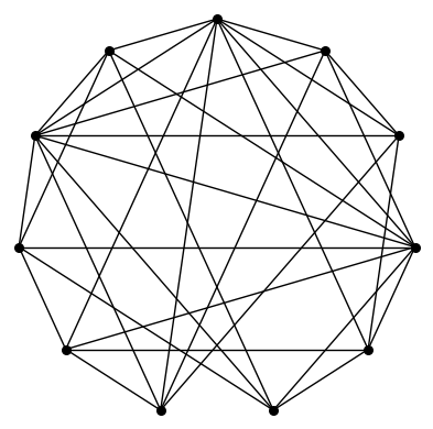
Figure 4. The graph of the combinatorially unique $5$-dimensional polytope that arises as the correlated equilibrium polytope of a $(2\times 3)$-game, as described in Theorem 5.9.

Proof.

First recall that the combinatorial type is fully determined by the sign patterns of the maximal minors of $A(Y)$, i.e. the oriented matroid of $A(Y)$. For $(2\times 3)$-games the matrix $A(Y)$ has 1206 nonzero maximal minors for generic $Y$, since $1797$ of the $\binom{14}{6}=3003$ maximal minors are identically zero. The signs of these 1206 maximal minors are completely determined by the signs of the irreducible components of $\det(A(Y)_{B})$ for each $B\in\binom{[14]}{6}$. As in Theorem 5.8 and Example 5.6, there are 12 such irreducible components $f_{1},\ldots,f_{12}$, which are given by the 9 coordinate hyperplanes and the 3 binomials listed in the example. This means that once we fix a sign pattern $s\in\{1,-1\}^{12}$ of the $f_{i}$ the signs of all maximal minors of $A(Y)$ are uniquely determined. Thus, to compute all possible combinatorial types, we compute the combinatorial type of the polytope once for each possible sign pattern $s$ of the $f_{i}(Y)$.

We do this computationally, using the software Mathematica 13.0 and SageMath 9.6 [Wol22, Sag22]. We first use Mathematica to find a payoff $Y\in\mathcal{S}$ such that $s_{i}f_{i}(Y)>0$ for all $i=1,\dots,12$. We then compute the corresponding combinatorial type of the polytope in SageMath. These computations can be found in the files combinatorialTypes2x3.nb and combinatorialTypes2x3.ipynb on MathRepo [MR22] respectively.

As a result we obtain $3$ different possible combinatorial types, which are a single point, the unique combinatorial type of full-dimensions of $(2\times 2)$-games (a bipyramid over a triangle), and a new unique full-dimensional combinatorial type. This polytope has $f$-vector $(1,11,32,40,25,8,1)$, and the graph of this $5$-dimensional polytope is depicted in Figure 4. A full description of this polytope can be found in combinatorialTypes2x3.ipynb on our MathRepo page [MR22]. ∎

Example 5.10 (Combinatorial types of $(2\times 3)$-games).

By Theorem 5.9, for $(2\times 3)$-games there is a unique combinatorial type of full-dimension. This is a $5$-dimensional polytope with $f$-vector $(1,11,32,40,25,8,1)$ and its graph is depicted in Figure 4.

Theorem 5.8 shows, that in $(2\times 3)$-games all correlated equilibrium polytopes that are not of maximal dimension appear as the maximal polytope of a smaller game. This gives rise to the following conjecture.

Conjecture 5.1.

Let $G$ be a $(2\times n)$-game with generic payoff matrices and let $P_{G}$ be its correlated equilibrium polytope. If $P_{G}$ is not of maximal dimension, then there exists a $(2\times k)$-game $G^{\prime}$ where $k<n$ such that $P_{G^{\prime}}$ is has maximal dimension and $P_{G}$ and $P_{G^{\prime}}$ are combinatorially equivalent.

Unique Combinatorial Types by Dimension
Dimension	0	3	5	7	9
$(2\times 2)$	1	1	0	0	0
$(2\times 3)$	1	1	1	0	0
$(2\times 4)$	1	1	1	3	0
$(2\times 5)$	1	1	1	3	4

Table 1. The number of unique combinatorial types of $P_{G}$ of each dimension for a $(2\times n)$-game in a random sampling of size $100\ 000$.

A relevant study to this conjecture is the dual reduction process of finite games. An iterative dual reduction reduces a finite game $G$ to a lower-dimensional elementary game $G^{\prime}$, for which $P_{G^{\prime}}$ is full-dimensional, by deleting certain pure strategies or merging several pure strategies into a single one. Any correlated equilibrium of the reduced game $G^{\prime}$ is a correlated equilibrium of the original game $G$, however the opposite is not always true [Mye97, Section 5]. 5.1 is supported by our computations thus far. To test this conjecture, we sampled $100\ 000$ random payoff matrices $X$ for $(2\times n)$-games for $n=4,5$. The results are summarized in Table 1, which shows the number of unique combinatorial types of a given dimension that we found for each $(2\times n)$-game. In all of our computations, 5.1 holds. The supporting code can be found on [MR22].

In contrast to the $(2\times n)$-case, $(2\times 2\times 2)$-games exhibit a much wider variety of distinct combinatorial types. In a sample of $100\ 000$ random payoff matrices for $(2\times 2\times 2)$-games, we found $14\ 949$ distinct combinatorial types which are of maximal dimension. Amongst these $7$-dimensional polytopes, the number of vertices can range from $8$ to $119$, the number of facets from $8$ to $14$, and the number of total faces from $256$ to $2338$. Examples of $f$-vectors achieving these bounds are

$$f_{P_{G_{1}}} =(1,8,28,56,70,56,28,8,1)$$

$$f_{P_{G_{2}}} =(1,119,458,728,616,302,87,14,1),$$

$$f_{P_{G_{3}}} =(1,119,460,733,620,303,87,14,1).$$

Affiliations

Marie-Charlotte Brandenburg
Max Planck Institute for Mathematics in the Sciences
Inselstr. 22, 04103 Leipzig, Germany
marie.brandenburg@mis.mpg.de

Benjamin Hollering
Max Planck Institute for Mathematics in the Sciences
Inselstr. 22, 04103 Leipzig, Germany
benjamin.hollering@mis.mpg.de

Irem Portakal
Technische Universität München
Boltzmannstr. 3, 85748 Garching b. München, Germany
mail@irem-portakal.de

References

[Aum74]
R. J. Aumann.
Subjectivity and correlation in randomized strategies.
Journal of Mathematical Economics, 1(1):67–96, 1974.
[Aum87]
R. J. Aumann.
Correlated equilibrium as an expression of bayesian rationality.
Econometrica, 55(1):1–18, 1987.
[Bas03]
Saugata Basu.
Different bounds on the different betti numbers of semi-algebraic
sets.
Discrete and Computational Geometry, 30(1):65–85, 2003.
[BLN22]
Saugata Basu, Antonio Lerario, and Abhiram Natarajan.
Betti numbers of random hypersurface arrangements.
Journal of the London Mathematical Society, 2022.
[CA03]
Antoni Calvó-Armengol.
The Set of Correlated Equilibria of 2 x 2 Games, October 2003.
Preprint.
[GS22]
Daniel R. Grayson and Michael E. Stillman.
Macaulay2, Version 1.20, 2022.
http://www.math.uiuc.edu/Macaulay2/.
[LSV11]
Ehud Lehrer, Eilon Solan, and Yannick Viossat.
Equilibrium payoffs of finite games.
Journal of Mathematical Economics, 47:48–53, 01 2011.
[Mye97]
Roger B. Myerson.
Dual reduction and elementary games.
Games and Economic Behavior, 21(1):183–202, 1997.
[NCH04]
Robert Nau, Sabrina Gomez Canovas, and Pierre Hansen.
On the geometry of nash equilibria and correlated equilibria.
International Journal of Games Theory, 32(4), August 2004.
[NJ50]
John F. Nash Jr.
Equilibrium points in n-person games.
Proceedings of the national academy of sciences, 36(1):48–49,
1950.
[PR05]
Christos H. Papadimitriou and Tim Roughgarden.
Computing equilibria in multi-player games.
In Proceedings of the sixteenth annual ACM-SIAM symposium on
discrete algorithms, SODA 2005, Vancouver, BC, Canada, January 23–25,
2005., pages 82–91. New York, NY: ACM Press, 2005.
[PR08]
Christos H Papadimitriou and Tim Roughgarden.
Computing correlated equilibria in multi-player games.
Journal of the ACM (JACM), 55(3):1–29, 2008.
[PS22]
Irem Portakal and Bernd Sturmfels.
Geometry of dependency equilibria.
Rend. Istit. Mat. Univ. Trieste, 54, Art. No. 5, 2022.
[PSA22]
Irem Portakal and Javier Sendra-Arranz.
Nash conditional independence curve.
arXiv preprint arXiv:2206.07000, 2022.
[Sag22]
The Sage Developers.
SageMath, the Sage Mathematics Software System
(Version 9.6), 2022.
https://www.sagemath.org.
[Spo03]
Wolfgang Spohn.
Dependency equilibria and the causal structure of decision and game
situation.
Homo Oeconomicus, 20:195–255, 2003.
[Stu02]
B. Sturmfels.
Solving systems of polynomial equations.
In American Mathematical Society, CBMS Regional Conferences
Series, No 97, 2002.
[Vio03]
Yannick Viossat.
Elementary Games and Games Whose Correlated Equilibrium Polytope Has
Full Dimension.
Preprint, 2003.
[Vio10]
Yannick Viossat.
Properties and applications of dual reduction.
Economic Theory, 44(1):53–68, 2010.
[Wol22]
Wolfram Research, Inc.
Mathematica, Version 13.0, 2022.