Slow and fast particles in shear-driven jamming: critical behavior

Abstract

We do extensive simulations of a simple model of shear-driven jamming in two dimensions to determine and analyze the velocity distribution at different densities $\phi$ around the jamming density $\phi_{J}$ and at different low shear strain rates, $\dot{\gamma}$. We then find that the velocity distribution is made up of two parts which are related to two different physical processes which we call the slow process and the fast process as they are dominated by the slower and the faster particles, respectively. Earlier scaling analyses have shown that the shear viscosity $\eta$, which diverges as the jamming density is approached from below, consists of two different terms, and we present strong evidence that these terms are related to the two different processes: the leading divergence is due to the fast process whereas the correction-to-scaling term is due to the slow process. The analysis of the slow process is possible thanks to the observation that the velocity distribution for different $\dot{\gamma}$ and $\phi$ at and around the shear-driven jamming transition, has a peak at low velocities and that the distribution has a constant shape up to and slightly above this peak. We then find that it is possible to express the contribution to the shear viscosity due to the slow process in terms of height and position of the peak in the velocity distribution and find that this contribution matches the correction-to-scaling term, determined through a standard critical scaling analysis. A further observation is that the collective particle motion is dominated by the slow process. In contrast to the usual picture in critical phenomena with a direct link between the diverging correlation length and a diverging order parameter, we find that correlations and shear viscosity decouple since they are controlled by different sets of particles and that shear-driven jamming is thus an unusual kind of critical phenomenon.

I Introduction

Particle transport is an ubiquitous phenomenon with relevance for both industry and every-day life and the behaviors of such real-life systems are immensely complicated as they include effects of e.g. varying particle shape, friction, and gravity. Even idealized systems O’Hern et al. (2003) where such complications can be eliminated—spherical (or circular) particles without any friction and well-controlled volume or pressure—remain poorly understood. Some salient features are that the shear viscosity increases as the packing fraction $\phi$ approaches the jamming packing fraction $\phi_{J}$ from below, that the relaxation time increases, and that the particle motion becomes increasingly correlated. It has however been difficult to find a way to connect together different quantities and behaviors into a comprehensive picture.

Simulations of shear-driven jamming are typically performed at constant packing fraction $\phi$ and low shear strain rates $\dot{\gamma}$ Durian (1995), and some of the quantities of interest are pressure $p$ and shear stress $\sigma$. One important characterization of the shear-driven jamming transition is through the value of the critical exponent $\beta$ that describes the divergence of the shear viscosity, $\eta\equiv\sigma/\dot{\gamma}$, as the jamming density $\phi_{J}$ is approached from below,

$$\eta\sim(\phi_{J}-\phi)^{-\beta}.$$ (1)

A starting point for many theoretical attempts to understand shear-driven jamming has been properties of static jammed packings at, or slightly above, jamming. A collection of particles with contact-only interactions forms a rigid network just at the jamming transition, with the number of contacts per particle equal to $z=z_{c}\equiv 2d$ Alexander (1998), (with the generalization to a finite number of particles in Ref. Goodrich et al. (2012)), and both the distance between close particles and the weak contact forces for contacting particles follow power-law distributions with non-trivial exponents Charbonneau et al. (2014a, b, 2015). From the values of these exponents, expected to be the same for dimension $d\geq 2$, together with some additional assumptions, one has found $\beta/u_{z}\approx 3.41$ DeGiuli et al. (2015); Ikeda (2020) for the exponent that describes the dependence of the viscosity on the distance to isostaticity, $\eta\sim(z-z_{c})^{-\beta/u_{z}}$. This may be compared with results from simulations in two dimensions that have generally given lower values: $\beta/u_{z}=1/0.38=2.63$ Lerner et al. (2012a) and $\beta/u_{z}=2.69$ Olsson (2015). (A later work by the group of Ref. Lerner et al. (2012a) gave a higher value, $\beta/u_{z}\approx 3.3$ DeGiuli et al. (2015), in agreement with the theoretical value, but that was for three dimensions ; determinations in two dimensions tend to give lower values Olsson (2019); Nishikawa et al. (2021); Olsson (2022).) Similarly, the values of $\beta$ in two dimensions, which have typically been in the range $\beta=2.2$ through 2.83 Andreotti et al. (2012); Olsson and Teitel (2011); Kawasaki et al. (2015) are found to be in agreement with the lower values ($\beta/u_{z}\approx 2.69$) when using $u_{z}=1$ Heussinger and Barrat (2009). One way to explain this discrepancy between the theoretically found $\beta/u_{z}\approx 3.41$ DeGiuli et al. (2015); Ikeda (2020) and the lower values from simulations is to claim that these lower values are incorrect due to a neglect of logarithmic corrections to scaling Ikeda (2020). This is a possibility since the upper critical dimension of the jamming transition is widely believed to be $d_{\mathrm{ucp}}=2$ Wyart et al. (2005); Goodrich et al. (2012), which opens up for logarithmic corrections to scaling. Though this explanation is a possibility, it could also be that the discrepancy only points to a lack of understanding of the phenomenon of shear-driven jamming.

Of the mentioned works, Ref. Lerner et al. (2012a) from simulations of hard disks, and the simulations that are based on relaxing configurations of soft disks below $\phi_{J}$ Olsson (2015, 2019); Nishikawa et al. (2021); Olsson (2022), determine the divergence in terms of $\delta z$, and do not give any value for $\phi_{J}$. The other works mentioned above are from simulations of soft disks Andreotti et al. (2012); Olsson and Teitel (2011); Kawasaki et al. (2015) and rely on scaling relations in one way or the other.

It has long been realized that the particle motion becomes increasingly collective as $\phi_{J}$ is approached from below Pouliquen (2004). One way to study this in simulations is with the overlap function Lechenault et al. (2008); Heussinger et al. (2010) and the associated dynamic susceptibility, $\chi_{4}$, which gives a measure of the number of particles that move collectively. With the assumption that the correlated domains have a compact geometry that quantity gave a length diverging with $\nu=0.9$; similar exponents were found also from other quantities Heussinger et al. (2010). From a correlation function that, in contrast to $\chi_{4}$, makes use of the vectorial nature of the velocity field, it has also been found that it is possible to extract two correlation lengths from the velocity fluctuations, respectively related to the rotation and the divergence of the velocity field. It appears that it is the length scale related to the rotations that is the more significant one Olsson and Teitel (2020).

With a diverging length scale and a diverging dynamic quantity, $\eta$, it could seem that the jamming transition fits nicely into the ordinary description of a critical phenomenon. It has however been difficult to understand the detailed connection between these two quantities. The divergence of the correlation length with $\nu=1$ has sometimes been taken to suggest $\beta=2$—one way to get that result is from the derivation of Eq. (31) in Sec. III.8 below—which is difficult to reconcile with the range of $\beta$ values given above.

In this paper we present evidence for, and explore some consequences of, the existence of two different processes in the system with different scaling properties: the fast process which is dominated by fast particles from the tail of the velocity distribution and the slow process which is dominated by the big fraction of slow particles from the peak of the distribution. It has already been shown that the divergence of the viscosity is dominated by a small fraction of particles with the highest velocities Olsson (2016), which means that the behavior described in Eq. (1) is controlled by the fast process. In this paper we show that the collective motion is governed by the slow process. A consequence is that the link between correlation length and the diverging shear viscosity is only an indirect one, which seems to imply that shear-driven jamming is a very unusual kind of critical phenomenon.

The analyses in the presented paper are for two-dimensional systems, only. Preliminary studies in three and four dimensions do however show that the same kind of analysis works very well also in these higher dimensions, and we therefore expect the conclusions to hold also in the more physically relevant case of three dimensions. These results will be presented elsewhere.

Though a critical divergence of a quantity as in Eq. (1) is described by a critical exponent there are usually additional terms that have to be included in the analyses unless one happens to have access to data only very close to the critical point. This goes under the heading of “corrections to scaling” and is due to the presence of irrelevant variables in the scaling function. In shear-driven jamming one has indeed found that a single diverging term cannot successfully fit the data Olsson and Teitel (2011); Kawasaki et al. (2015) and the inclusion of a correction-to-scaling term was found to give reasonable analyses. The finding of two different processes in shear-driven jamming, however, opens up for a different interpretation of this additional term. The evidence suggests that the correction-to-scaling term is due to the slow process which means that it is possible to relate this term to a separate physical process, which is unusual for critical phenomena.

The remainder of the paper is organized as follows: In Sec. II we describe the simulations and the measured quantities and give a motivation for the use of the velocity distribution for analyzing shear-driven jamming. We also review the scaling relations and discuss shortly different ways to analyze the transition. In Sec. III we describe the results, to a large extent through analyses of data at $\phi\approx\phi_{J}$. We do this by first showing that the correction-to-scaling term of the shear stress may be related to the properties of the peak in the velocity distribution. We then first turn to the behavior at densities in a (narrow) interval around $\phi_{J}$ and show that the two different terms—where one is the contribution to $\sigma$ from the peak in the distribution and the other is the remainder—both scale with $\phi-\phi_{J}$ and $\dot{\gamma}$. We then also show that the same kind of analysis may actually be used also in the hard disk limit, i.e. in the region well below $\phi_{J}$ and at sufficiently low $\dot{\gamma}$ that the shear viscosity is independent of shear rate. We also discuss the origin of the high velocities of the fast process and then turn to the collective particle motion and argue that the diverging correlation length and the leading divergence of the shear viscosity, as jamming is approached, are due to different sets of particles. We then present a rationalization of some of our findings. In Sec. IV we finally summarize the results, discuss some open questions and some connections between our findings and the literature, and sketch a few directions for future research.

A jointly published Letter joi (2022) summarizes some of our key results. The Letter also shortly discusses finite size scaling, which will be discussed in more detail in a separate publication.

II Models and measured quantities

II.1 Simulations

For the simulations we follow O’Hern et al. O’Hern et al. (2003) and use a simple model of bi-disperse frictionless disks in two dimensions with equal numbers of particles with two different radii in the ratio 1.4. We use Lees-Edwards boundary conditions Evans and Morriss (1990) to introduce a time-dependent shear strain $\gamma=t\dot{\gamma}$. With $r_{ij}$ the distance between the centers of two particles and $d_{ij}$ the sum of their radii, the relative overlap is $\delta_{ij}=1-r_{ij}/d_{ij}$ and the interaction between overlapping particles is $V_{p}(r_{ij})=\epsilon\delta_{ij}^{2}/2$; we take $\epsilon=1$. The force on particle $i$ from particle $j$ is $\mathbf{f}^{\mathrm{el}}_{ij}=-\nabla_{i}V_{p}(r_{ij})$, which gives the force magnitude $f^{\mathrm{el}}_{ij}=\epsilon\delta_{ij}/d_{ij}$. The total elastic force on a particle is $\mathbf{f}^{\mathrm{el}}_{i}=\sum_{j}\mathbf{f}^{\mathrm{el}}_{ij}$ where the sum is over all particles $j$ in contact with $i$.

The simulations discussed here have been done at zero temperature with the RD₀ (reservoir dissipation) model Vågberg et al. (2014a) with the dissipating force $\mathbf{f}^{\mathrm{dis}}_{i}=-k_{d}\mathbf{v}_{i}$ where $\mathbf{v}_{i}\equiv\mathbf{v}_{i}^{\mathrm{tot}}-y_{i}\dot{\gamma}\hat{x}$ is the non-affine velocity, i.e. the velocity with respect to a uniformly shearing velocity field, $y_{i}\dot{\gamma}\hat{x}$. In the overdamped limit the equation of motion is $\mathbf{f}^{\mathrm{el}}_{i}+\mathbf{f}^{\mathrm{dis}}_{i}=0$ which becomes $\mathbf{v}_{i}=\mathbf{f}^{\mathrm{el}}_{i}/k_{d}$. We take $k_{d}=1$ and the time unit $\tau_{0}=d_{s}^{2}k_{d}/\epsilon=1$. Length is measured in units of the diameter of the small particles, $d_{s}$. The equations of motion were integrated with the Heuns method with time step $\Delta t/\tau_{0}=0.2$. Unless otherwise noted the results are for $N=65536$ particles.

II.2 Measured quantities

Using $\mathbf{r}_{ij}=\mathbf{r}_{i}-\mathbf{r}_{j}$ we determine the pressure tensor,

$$\mathbf{p}^{\mathrm{el}}=\frac{1}{V}\sum_{i<j}\mathbf{f}^{\mathrm{el}}_{ij}\otimes\mathbf{r}_{ij},$$ (2)

which is measured during the simulations once per unit time. Here $V=L\times L$ is the volume. The pressure is obtained from the pressure tensor through

$$p=\frac{1}{2}[\left<\mathbf{p}^{\mathrm{el}}_{xx}\right>+\left<\mathbf{p}^{\mathrm{el}}_{yy}\right>],$$

and the shear stress is given by

$$\sigma=-\left<\mathbf{p}^{\mathrm{el}}_{xy}\right>.$$ (3)

The analyses below will focus on the dissipation and a crucial relation is then the connection between shear stress and $\left<v^{2}\right>$ (where $v\equiv|\mathbf{v}|$ is the non-affine velocity) which follows from the requirement of power balance between the input power $V\sigma\dot{\gamma}$ and the dissipated power $k_{d}\sum v_{i}^{2}$, where the sum is over all the particles. This gives Ono et al. (2003)

$$\sigma\dot{\gamma}=\frac{N}{V}k_{d}\left<v^{2}\right>,$$ (4)

which implies $\sigma\sim\left<v^{2}\right>/\dot{\gamma}$.

II.3 The velocity distribution

Though Eq. (4) could lead to the thinking that measures of the velocity and measures of $\sigma$ only give the same information, our claim is there is more information in the velocity distribution. To see this we consider the behavior of continuously sheared hard spheres below $\phi_{J}$. For that case it has been found that the displacement (i.e. velocity) is governed by steric exclusion Andreotti et al. (2012) and that the forces at each moment will adjust to give the velocities that are required by steric hindrance. This implies that the forces and the shear stress are controlled by the velocity and it also suggests that velocity is a more fundamental quantity, and that there might be more information in the full velocity distribution than what is contained in the shear stress, $\sigma$. In the present work we set out to extract some of that information.

To measure the distribution function ${\cal P}(v)$ we define the bin size $\Delta$ and $v_{k}=k\Delta$ and let the histogram $H(v_{k})$ be the fraction of the non-affine particle velocities in the range $[v_{k}-\Delta/2,v_{k}+\Delta/2)$. Histograms are created from files with configurations that are stored every 10 000 time step. The distribution function, ${\cal P}(v_{k})=H(v_{k})/\Delta$, is normalized such that $\int{\cal P}(v)dv=1$. From Eq. (4) follows an expression for the shear stress in terms of the velocity distribution function,

$$\sigma=\frac{N}{V}\frac{k_{d}}{\dot{\gamma}}\int{\cal P}(v)v^{2}dv.$$ (5)

II.4 Scaling relations

For easy reference we here show derivations of some scaling relations from the standard scaling assumption Olsson and Teitel (2007); Vågberg et al. (2016),

$$\sigma(\phi,\dot{\gamma})b^{y/\nu}=\bar{g}_{\sigma}(\delta\phi\,b^{1/\nu},\dot{\gamma}b^{z})+b^{-\omega}\bar{h}_{\sigma}(\delta\phi\,b^{1/\nu},\dot{\gamma}b^{z}).$$ (6)

Here $b$ is a length rescaling factor, $y$ is the scaling dimension of $\sigma$, $\nu$ is the correlation length exponent, $\delta\phi=\phi-\phi_{J}$, $z$ is the dynamical exponent, $\omega$ is the correction-to-scaling exponent and $\bar{g}_{\sigma}$ and $\bar{h}_{\sigma}$ are unknown scaling functions.

With $b=\dot{\gamma}^{-1/z}$ in Eq. (6) and with $q=y/z\nu$ one finds

$$\sigma(\phi,\dot{\gamma})=\dot{\gamma}^{q}\left[g_{\sigma}\left(\frac{\phi-\phi_{J}}{\dot{\gamma}^{1/z\nu}}\right)+\dot{\gamma}^{\omega/z}h_{\sigma}\left(\frac{\phi-\phi_{J}}{\dot{\gamma}^{1/z\nu}}\right)\right].$$ (7)

One way to determine the critical behavior of the shear-driven jamming transition has been to fit $\sigma(\phi,\dot{\gamma})$ or $p(\phi,\dot{\gamma})$ at densities around $\phi_{J}$, to this expression Olsson and Teitel (2011). The scaling functions $g_{\sigma}$ and $h_{\sigma}$ were there taken to be exponentials of polynomials in $(\phi-\phi_{J})/\dot{\gamma}^{1/z\nu}$, and both $\phi_{J}$ and the critical exponents were determined through scaling fits of both $p$ and $\sigma$.

Right at $\phi_{J}$, with the notation $q_{2}=q+\omega/z$, Eq. (7) becomes

$$\sigma(\phi_{J},\dot{\gamma})=\dot{\gamma}^{q}g_{\sigma}(0)+\dot{\gamma}^{q_{2}}h_{\sigma}(0).$$ (8)

The conclusion of a behavior as in Eq. (8) was reached in a different way in Ref. Kawasaki et al. (2015). An analysis, consistent with Eq. (8), of a similar model, commonly used for granular materials, has also been done Rahbari et al. (2018).

To get the scaling relation for the shear viscosity one writes an expression for $\sigma(\phi,\dot{\gamma})b^{y/\nu}/(\dot{\gamma}b^{z})$ from Eq. (6) and takes $b=(-\delta\phi)^{-\nu}$. This then becomes

$$\eta(\phi,\dot{\gamma}) = (\phi_{J}-\phi)^{-\beta}g_{\eta}\left(\frac{\dot{\gamma}}{(\phi_{J}-\phi)^{z\nu}}\right)+$$ (9)

$$+ (\phi_{J}-\phi)^{-\beta_{2}}h_{\eta}\left(\frac{\dot{\gamma}}{(\phi_{J}-\phi)^{z\nu}}\right),$$

where $\beta=z\nu-y$ and $\beta_{2}=z\nu-y-\omega\nu$. The first term is the leading divergence and the second is the correction to scaling term. When comparing with the expressions for $q$ and $q_{2}$ in Eq. (8) one finds

$$\beta/z\nu = 1-q,$$ (10a)

$$\beta_{2}/z\nu = 1-q_{2}.$$ (10b)

For sufficiently small $\dot{\gamma}$ the scaling functions in Eq. (9) approach constants, and one arrives at

$$\eta(\phi,\dot{\gamma}\to 0)=c_{1}(\phi_{J}-\phi)^{-\beta}+c_{2}(\phi_{J}-\phi)^{-\beta_{2}},$$ (11)

which is the behavior in the hard disk limit.

One approach to shear-driven jamming is then to consider the shearing of a collection of hard disks (or soft disk in the limit $\dot{\gamma}\to 0$) below $\phi_{J}$, and thus with the average number of contacts $z<z_{c}$. This is sometimes called the floppy flow regime. Another approach, relevant at higher shear strain rates and/or closer to $\phi_{J}$, is to examine the behavior where the elasticity of the particles is important. This is the elasto-plastic regime which at $\phi_{J}$ is described by Eq. (8). Though it could seem that the behaviors in these different regimes are governed by very different physical processes, we note that the respective behaviors both follow from a single scaling assumption, which suggests that both regions are governed by the same fundamental physics.

The present article presents a novel analysis of the shear-driven jamming transition. Most of the analyses are done on data at $\phi=\phi_{J}$ and for different $\dot{\gamma}$, but in Sec. III.5 we demonstrate that the same kind of analysis works well also for data in the hard disk limit at $\phi<\phi_{J}$.

III Results

III.1 Two terms in $\sigma$

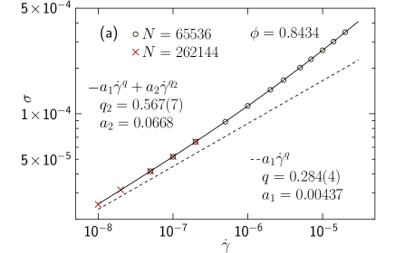
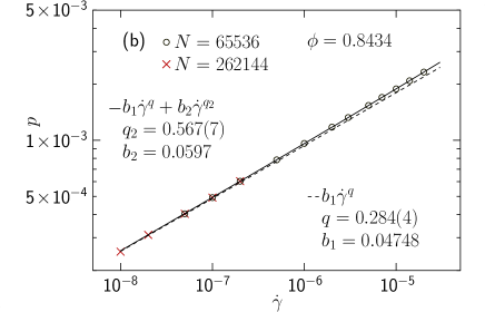
Figure 1: Determination of the exponents $q$ and $q_{2}$ that characterize the two terms in the shear stress. The figures show results from simultaneous fits of $\sigma$ and $p$ at $\phi=0.8434\approx\phi_{J}$ to Eqs. (12) and (13), demanding that both $q$ and $q_{2}$ are the same, i.e. $q_{2}^{(p)}=q_{2}$—method C of Appendix A. Panels (a) and (b) show $\sigma(\phi_{J},\dot{\gamma})$ and $p(\phi_{J},\dot{\gamma})$. The dashed lines are the main terms, $\sim\dot{\gamma}^{q}$, whereas the solid lines are the full expressions. The simpler approach to fit $\sigma(\phi_{J},\dot{\gamma})$ to Eq. (12), only—this is method A of Appendix A—gives just slightly different values of $q$ and $q_{2}$. Note that the size of the secondary terms, in absolute terms, is about the same for both quantities, as $b_{2}\approx a_{2}$. The relative size of the secondary term is however considerably smaller for $p$ than for $\sigma$.

The focus of the present paper is not on the values of the exponents and the main conclusion from Eq. (7) is that the shear stress consists of two terms. In the analyses below we will take $\phi_{J}\approx 0.8434$ Heussinger and Barrat (2009); Olsson and Teitel (2011). We write Eq. (8) as

$$\sigma(\phi_{J},\dot{\gamma})=a_{1}\dot{\gamma}^{q}+a_{2}\dot{\gamma}^{q_{2}}\equiv\sigma_{1}(\phi_{J},\dot{\gamma})+\sigma_{2}(\phi_{J},\dot{\gamma}).$$ (12)

It is now perfectly possible to determine the exponents $q$ and $q_{2}$ by fitting $\sigma(\phi_{J},\dot{\gamma})$ to the middle expression of Eq. (12), but in order to get higher precision in the determinations we follow Ref. Rahbari et al. (2018) and make use of the expectation that the same exponents should be present also in the analogous expression for the pressure,

$$p(\phi_{J},\dot{\gamma})=b_{1}\dot{\gamma}^{q}+b_{2}\dot{\gamma}^{q^{(p)}_{2}}.$$ (13)

The simultaneous fits of $\sigma(\phi_{J},\dot{\gamma})$ and $p(\phi_{J},\dot{\gamma})$ with this approach, when taking $q^{(p)}_{2}=q_{2}$, are shown in Fig. 1, and gives the exponents

$$q = 0.284(4),$$

$$q_{2} = 0.567(7).$$

The error estimates correspond to three standard deviations. More details on this approach and some similar methods are given in Appendix A

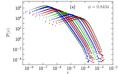
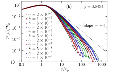
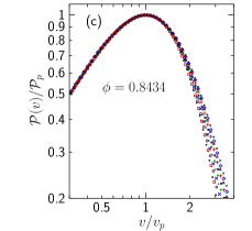
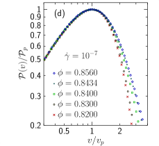
Figure 2: Velocity distribution at $\phi=0.8434\approx\phi_{J}$ and several different shear strain rates. Panel (a) gives ${\cal P}(v)$ for several different shear strain rates. As is clear from panel (a) each data set has a clear peak and panel (b) shows the same data rescaled to make the peaks coincide. It is then found that the rescaled ${\cal P}(v)$ collapse below and up to the peak whereas the data above the peak depend strongly on $\dot{\gamma}$. Panel (c) is a zoom-in on the data of panel (b). Panel (d) shows that the same kind of collapse is found also for ${\cal P}(v)$ at $\dot{\gamma}=10^{-7}$ for $\phi$ both below and above $\phi_{J}$.

III.2 Scaling of the peak properties

The velocity distributions at $\phi=0.8434\approx\phi_{J}$ and for a range of different shear strain rates from $\dot{\gamma}=1\times 10^{-8}$ through $2\times 10^{-5}$ are shown in Fig. 2(a). [Since these figures with double-log scale are not immediately amenable for simple interpretation, Appendix B shows both ${\cal P}(v)$ and a few other quantities on both logarithmic and linear scales.] At each $\dot{\gamma}$ there is a peak in ${\cal P}(v)$ at low velocities and we identify peak height ${\cal P}_{p}$ and peak position $v_{p}$. These quantities are then used to rescale both axes in the figure such that the peaks fall on top of each other and, as shown in Fig. 2(b) and in the zoomed-in Fig. 2(c), these data collapse nicely up to and slightly above the peak. The same kind of behavior is found for ${\cal P}(v)$ also at densities away from $\phi_{J}$ which is clear from Fig. 2(d) which shows the same kind of data for $\dot{\gamma}=10^{-7}$ and $\phi=0.82$, 0.83, 0.84, 0.8434, and 0.8560. This therefore suggests that the low-velocity part of the distribution is governed by a simple dynamics with a robust behavior that gives a similar shape of the distribution independent of detailed properties of the system, as e.g. number of contacts. This is in clear contrast to the behavior above the peak where the distributions are algebraic, $P(v)\sim v^{-r}$, with an exponent that changes with $\dot{\gamma}$ and $\phi$ and appears to approch $r=3$ at criticality Olsson (2016). (The distributions are eventually cut off exponentially, which is an effect of the finite strength of the contact forces that puts a limit on the total net force and thereby on the velocity Olsson (2016).)

To capture the velocity dependence in the expression for $\sigma$, Eq. (5), we now introduce $S(v)$ which is the contribution to $\sigma$ from the velocities up to $v$:

$$S(v)=\frac{N}{V}\frac{k_{d}}{\dot{\gamma}}\int_{0}^{v}{\cal P}(v^{\prime})v^{\prime 2}dv^{\prime}.$$ (14)

After introducing $x=v/v_{p}$ and $f(x)={\cal P}(v)/{\cal P}_{p}$ the contribution to $\sigma$ for velocities up to the peak, i.e. for all $v<v_{p}$, becomes

$$S(v_{p})=\frac{N}{V}k_{d}W_{p}\int_{0}^{1}f(x)x^{2}dx,$$ (15)

which shows that the dependency on $\phi$ and $\dot{\gamma}$ is only through the peak properties given by $W_{p}={\cal P}_{p}v_{p}^{3}/\dot{\gamma}$, because the curves for different $\dot{\gamma}$ and $\phi$ collapse for $v\leq v_{p}$.

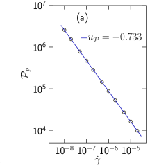
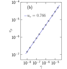
Figure 3: Peak properties at $\phi=0.8434\approx\phi_{J}$ from Fig. 2 and determinations of the related exponents. Panel (a) is the peak height, ${\cal P}_{p}$, whereas panel (b) is the (velocity) position of the peak, $v_{p}$.

Fig. 3, which is again obtained at $\phi=0.8434\approx\phi_{J}$, shows that both ${\cal P}_{p}$ and $v_{p}$ depend algebraically on $\dot{\gamma}$ to very good approximations. We find

$${\cal P}_{p}(\phi_{J},\dot{\gamma}) \sim \dot{\gamma}^{u_{{\cal P}}},\quad u_{{\cal P}}=-0.733,$$ (16a)

$$v_{p}(\phi_{J},\dot{\gamma}) \sim \dot{\gamma}^{u_{v}},\quad u_{v}=0.766.$$ (16b)

For $W_{p}\equiv{\cal P}_{p}v_{p}^{3}/\dot{\gamma}$ this gives

$$W_{p}(\phi_{J},\dot{\gamma})\sim\dot{\gamma}^{u_{{\cal P}}}\dot{\gamma}^{3u_{v}}\dot{\gamma}^{-1}\sim\dot{\gamma}^{u_{w}},$$ (17)

with

$$u_{w}\equiv 3u_{v}+u_{\cal P}-1=0.565,$$ (18)

which is in very good agreement with $q_{2}\approx 0.567$ from the fit of $\sigma(\phi_{J},\dot{\gamma})$ to Eq. (12). This therefore suggests that the secondary term, $\sigma_{2}$, is related to the slow particles in the peak of the distribution.

III.3 Magnitude of $\sigma_{s}$

We now split the velocity distribution into two terms for the two different processes, dominated by slow and fast particles, respectively,

$${\cal P}(v)={\cal P}_{s}(v)+{\cal P}_{f}(v),$$ (19)

where we take ${\cal P}_{s}(v)={\cal P}(v)$, for $v\leq v_{p}$. To get a clue to the shape of ${\cal P}_{s}(v)$ above the peak, we turn to Fig. 4 which shows the velocity distribution at lower densities, $\phi=0.76$, 0.80, and 0.82. It is there found that the high-velocity tail shrinks away as $\phi$ is lowered and apparently vanishes at $\phi=0.76$, shown in Fig. 4(a). What remains is an exponentially decaying ${\cal P}(v)$ and we take this as a guidance for constructing ${\cal P}_{s}(v)$ above the peak at general $\phi$.

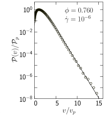
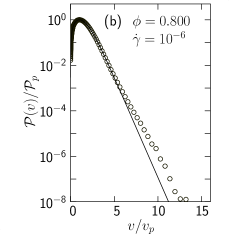
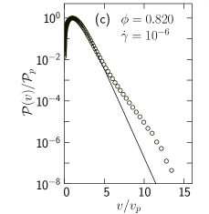
Figure 4: Rescaled velocity distributions at low densities, $\phi=0.76$, 0.80, and 0.82. Note that the $x$ axes have linear scales, in contrast to the logarithmic scales in Fig. 2. At the lowest density, $\phi=0.76$, in panel (a), the distribution is exponential whereas there start to develop deviations from that behavior at the higher densities in panels (b) and (c). We gather that the exponential decay is the characteristics of the slow process whereas the deviations from that behavior develop into the algebraic tails of Fig. 2 that characterize the fast process.

Defining $\sigma_{s}$ to be the contribution to $\sigma$ from ${\cal P}_{s}(v)$,

$$\sigma_{s}=\frac{N}{V}\frac{k_{d}}{\dot{\gamma}}\int{\cal P}_{s}(v)v^{2}dv,$$

and using the same kind of reasoning as in Eq. (15), we introduce $f_{s}(x)={\cal P}_{s}(v)/{\cal P}_{p}$ and find

$$\sigma_{s}=\frac{N}{V}k_{d}W_{p}\int f_{s}(x)x^{2}dx=\frac{N}{V}k_{d}W_{p}I_{2},$$ (20)

where $I_{2}$ is the integral,

$$I_{2}\equiv\int f_{s}(x)\;x^{2}\;dx.$$ (21)

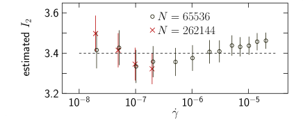
Figure 5: Estimates of $I_{2}$ from Eq. (22). The input for these data are both estimates of $\sigma_{2}(\phi_{J},\dot{\gamma})\equiv\sigma(\phi_{J},\dot{\gamma})-a_{1}\dot{\gamma}^{q}$ and $W_{p}(\phi_{J},\dot{\gamma})$ from the velocity distributions. Beside the displayed error bars, which show one standard deviation, an important source of error is the uncertainty in $\phi_{J}$. The present estimate is based on assuming $\phi_{J}=0.843~{}43$ as obtained in Appendix A.

To determine the numerical value of $I_{2}$ we assume $\sigma_{s}=\sigma_{2}$ and determine $\sigma_{2}$ from $\sigma_{2}=\sigma-a_{1}\dot{\gamma}^{q}$ with $a_{1}$ and $q$ from the fit to Eq. (12) to get

$$I_{2}=\frac{V}{N}\;\frac{[\sigma(\phi_{J},\dot{\gamma})-a_{1}\dot{\gamma}^{q}]}{k_{d}\;W_{p}(\phi_{J},\dot{\gamma})},$$ (22)

which is shown in Fig. 5. Since the size of the secondary term depends sensitively on the assumed $\phi_{J}$ we here make use of $\phi_{J}=0.843~{}43$ obtained in Appendix A. Here $\sigma(\phi_{J},\dot{\gamma})$ from Eq. (3) together with $W_{p}(\phi_{J},\dot{\gamma})$ from the peak properties give estimates of $I_{2}$ for different $\dot{\gamma}$. We note that the different estimates of $I_{2}$ are encouragingly similar and give $I_{2}\approx 3.4$. (The error bars in Fig. 5 are due to the uncertainties in $a_{1}$ and $q$ in the fit to Eq. (12).)

We now take $f_{s}(x)$ to be given by the rescaled distributions up to (and slightly above) the peak and assume an exponentially decaying $f_{s}(x)$ for $x>1$, and adjust the exponentially decaying part of $f_{s}(x)$ to give $I_{2}=3.4$, when integrated with Eq. (21). The outcome of this procedure is the dashed line in Fig. 6 which shows a possible shape of $f_{s}(x)$.

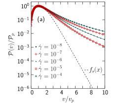
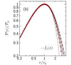
Figure 6: Possible shape of $f_{s}(x)$ together with data for shear rates $\dot{\gamma}=10^{-8}$ through $10^{-4}$. Panel (a) shows the exponential decay of $f_{s}(x)$ whereas the zoom-in in panel (b) shows the same data close to the peak.

Before continuing it is worth pointing out that the reasoning above rests on the assumption that ${\cal P}(v)$ up to the peak is altogether governed by the slow process. Even though this leads to a consistent picture it should be stressed that there is of course nothing to preclude the possibility that the distribution for the fast process actually is small but non-zero at $v=v_{p}$.

III.4 Behavior at densities around $\phi_{J}$

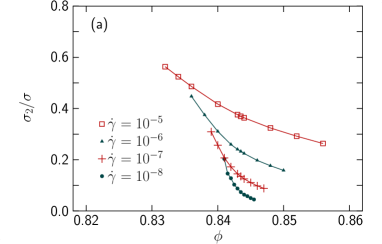
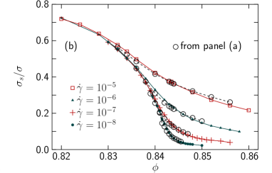
Figure 7: Comparison of $\sigma_{2}/\sigma$ and $\sigma_{s}/\sigma$ from two very different analyses. Panel (a) is from the scaling collapse according to Eq. (7) where $\sigma_{2}$, as defined in Eq. (12), is the secondary, correction-to-scaling, term. Panel (b) is $\sigma_{s}$ from the peak properties through Eq. (20) with $I_{2}=3.4$. The open circles connected with a dashed line are the values from panel (a). The great similarity of the two quantities suggest that they are related.

After the analyses of the behavior at $\phi\approx\phi_{J}$ we now turn to the behavior also away from $\phi_{J}$. The aim is not to get reliable determinations of the critical exponents—such determinations would require both estimates of the uncertainties in $W_{p}$ and a better understanding of the finite size effects on $\sigma_{s}$—but rather to show that $\sigma_{s}$ from the peak properties through $W_{p}$ and Eq. (20) behaves the same as the secondary term from Eq. (7),

$$\sigma_{2}=\dot{\gamma}^{q_{2}}h_{\sigma}\left(\frac{\phi-\phi_{J}}{\dot{\gamma}^{1/z\nu}}\right),$$ (23)

also away from $\phi_{J}$. Figures 7(a) and (b) show the relative contributions of $\sigma_{2}$ and $\sigma_{s}$ and it is clear that they are very similar. Note that $\sigma_{2}$—determined from the fit of $\sigma(\phi,\dot{\gamma})$ to Eq. (7)—is only available for the range of data that can be used for the fit whereas $\sigma_{s}$ can be determined from the peak of the velocity distribution for all data.

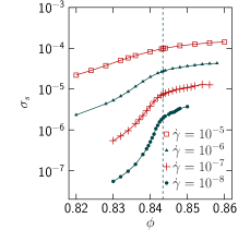
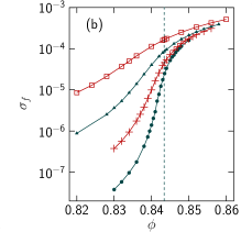
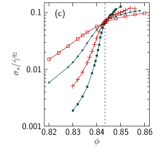
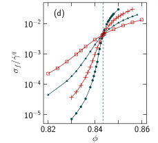
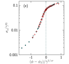
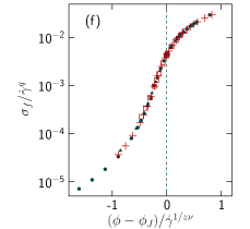
Figure 8: Raw data and scaling analyses of $\sigma_{s}$ and $\sigma_{f}\equiv\sigma-\sigma_{s}$. The vertical dashed lines are $\phi=0.8434\approx\phi_{J}$. For clarity we show data for the four shear strain rates, only: $\dot{\gamma}=10^{-8}$, $10^{-7}$, $10^{-6}$, and $10^{-5}$. Panels (a) and (b) are the raw $\sigma_{s}$ vs $\phi$ and $\sigma_{f}$ vs $\phi$. Panels (c) and (d) are the same quantities but scaled by $\dot{\gamma}^{q_{2}}$ and $\dot{\gamma}^{q}$, respectively, which make the data cross at $\phi_{J}$. Panels (e) and (f) are after also rescaling the $x$ axis to make the data collapse. Note that $\sigma_{s}$ are directly from the peak properties as the value of $I_{2}$ just enters as a trivial rescaling parameter. $\sigma_{f}$, on the other hand, also depends on the value of $I_{2}$ since it controls the size of the amounts subtracted from $\sigma$, as shown in Eqs. (20) and (24).

The identification of $\sigma_{2}$ with $\sigma_{s}$ means that we should expect $\sigma_{s}$ to scale with the exponent $q_{2}\equiv q+\omega/z$. We introduce $\sigma_{f}$ which is the contribution to $\sigma$ due to the fast process,

$$\sigma_{f}\equiv\sigma-\sigma_{s}.$$ (24)

This quantity should—just as the main term—scale with the exponent $q$. Fig. 8 shows $\sigma_{s}$ and $\sigma_{f}$ vs $\phi$ for $\dot{\gamma}=10^{-8}$ through $10^{-5}$. Panels (a) and (b) are the raw data, panels (c) and (d) are the same data rescaled by $\dot{\gamma}^{q_{2}}$ and $\dot{\gamma}^{q}$, and panels (e) and (f) show the attempted data collapses when plotted vs $(\phi-\phi_{J})/\dot{\gamma}^{1/z\nu}$ with $\phi_{J}=0.8434$ and $1/z\nu=0.26$ Olsson and Teitel (2011). The scaling collapses are very good.

Generally speaking the conclusions arrived at in this way match the results from Ref. Olsson and Teitel (2011). One notable point in Ref. Olsson and Teitel (2011) is that $q>1/z\nu$ which implies that $\sigma(\phi,\dot{\gamma}\to 0)\sim(\phi-\phi_{J})^{y}$ where $y=qz\nu>1$. Though more detailed scaling analyses of $\sigma_{f}$ and $\sigma_{s}$ will have to be deferred to a later paper, we can still attempt a determination of $1/z\nu$ from $\sigma_{f}(\phi_{J},\dot{\gamma})$. This is done by noting that $\sigma_{1}=\dot{\gamma}^{q}g_{\sigma}((\phi-\phi_{J})/\dot{\gamma}^{1/z\nu})$ from Eq. (7) implies that

$$\left.\frac{d\ln\sigma_{1}(\phi,\dot{\gamma})}{d\phi}\right|_{\phi_{J}}\sim\dot{\gamma}^{-1/z\nu}.$$ (25)

To estimate $1/z\nu$ we take $\sigma_{1}=\sigma_{f}$ and determine the above derivative for different shear strain rates $10^{-8}\leq\dot{\gamma}\leq 2\times 10^{-5}$ by fitting $\ln\sigma_{f}$ to second order polynomials in $\phi-\phi_{J}$ for data from narrow intervals around $\phi_{J}$, $|\phi-\phi_{J}|/\dot{\gamma}^{0.26}<0.3$. From the $\dot{\gamma}$ dependence of the term linear in $\phi-\phi_{J}$ we find $1/z\nu\approx 0.263$ and (with $q=0.284$) $y=qz\nu\approx 1.08$, in agreement with Ref. Olsson and Teitel (2011). It should be noted that the present approach is much more direct than the scaling analysis Olsson and Teitel (2011) that handles the secondary term through a complicated fitting. In the present approach that term is eliminated through the peak properties $W_{p}(\phi,\dot{\gamma})$ and the single parameter $I_{2}$ from Eq. (22).

III.5 Behavior at $\phi<\phi_{J}$ as $\dot{\gamma}\to 0$

The analyses above are for densities where elasto-plastic processes are important such that the viscosity is highly rate-dependent and it is interesting to also examine the behavior in the hard particle region where the viscosity is independent of shear strain rate. This is reached by taking sufficiently small $\dot{\gamma}$ at $\phi<\phi_{J}$. From the scaling picture one expects the same analysis to apply also for hard particles below $\phi_{J}$, and we here explicitely demonstrate that that actually is the case.

To approach the hard disk limit we have done simulations of soft disks at densities $\phi=0.830$ through 0.838 and shear strain rate $\dot{\gamma}=10^{-8}$ such that the average overlap of contacting particles is $<10^{-5}d_{s}$, which means that the simulations are indeed very close to the hard disk limit. From Fig. 9 which is ${\cal P}(v)$ both at five densities $\leq 0.838$, well below $\phi_{J}$, and at $\phi=0.8434\approx\phi_{J}$ we first note that there is no qualitative difference between the velocity distribution at $\phi_{J}$, where the elastic effects are important, and the distribution well below $\phi_{J}$, characteristic of the hard disk limit.

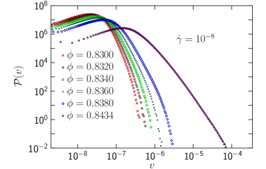
Figure 9: Velocity distributions at the low shear strain rate $\dot{\gamma}=10^{-8}$ both at five densities $\phi=0.830$ through 0.838 representative of the hard disk limit and the jamming density, $\phi=0.8434\approx\phi_{J}$. The properties of the peaks determine $W_{p}={\cal P}_{p}v_{p}^{3}/\dot{\gamma}$ which are used in Eq. (20) with $I_{2}=3.4$ to estimate $\sigma_{s}$.

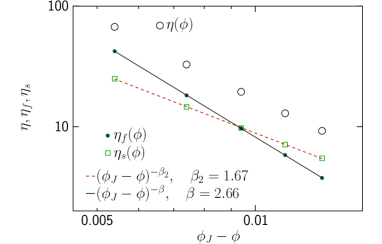
Figure 10: Analyses of the shear viscosity for data in the hard disk limit, $\dot{\gamma}=10^{-8}$ and $\phi=0.830$ through 0.838. The open circles are $\eta=\sigma/\dot{\gamma}$, the open squares are $\eta_{s}\equiv\sigma_{s}/\dot{\gamma}$ with $\sigma_{s}$ from the properties of the velocity distributions, as discussed in the caption of Fig. 9. The filled circles are $\eta_{f}\equiv\sigma_{f}/\dot{\gamma}$, where $\sigma_{f}=\sigma-\sigma_{s}$. The fit of $\eta_{s}$ to an algebraic divergence gives $\beta_{2}=1.67$ whereas the fit of $\eta_{f}$ gives $\beta=2.66$. As discussed in the main text these values are in good agreement with the corresponding values of $q_{2}$ and $q$ from the analyses of data at $\phi_{J}$.

Figure 10 shows our results for the viscosity in the hard particle limit. The open circles are $\eta\equiv\sigma/\dot{\gamma}$ with $\sigma$ from Eq. (3). The open squares are $\eta_{s}\equiv\sigma_{s}/\dot{\gamma}$ where $\sigma_{s}$ is determined with Eq. (20) with $W_{p}={\cal P}_{p}v_{p}^{3}/\dot{\gamma}$ from the properties of the peak together with the value $I_{2}=3.4$. The solid dots are the contribution from the fast particles $\eta_{f}=\eta-\eta_{s}$. As shown in Fig. 10 the values for these exponents from the fitting of $\eta_{s}$ and $\eta_{f}$ below $\phi_{J}$ to the algebraic divergences (given by the two terms in Eq. (11)) are $\beta=2.66$ and $\beta_{2}=1.67$, in very good agreement with $\beta=2.75$ and $\beta_{2}=1.67$ from Eq. (10), $1/z\nu=0.26$, and the values of $q$ and $q_{2}$ given below Eq. (13).

The conclusion from the section is thus that the splitting of data into slow and fast particles works the same for hard particles as for the data around $\phi_{J}$ and also that these different determinations of the exponents are in very good agreement.

III.6 Fast particles

After this comparison of the properties of the peak in the velocity distribution and the secondary term, as determined from the scaling analysis of $\sigma(\phi_{J},\dot{\gamma})$ together with an analysis in the hard disk limit below $\phi_{J}$, we now turn to the high velocity regime and the main process, to try to understand the origin of the highest velocities far out in the tail of the distribution. To that end we have examined several configurations with fast particles at density $\phi=0.80$. A typical case is as in Fig. 11(a), where the fast particle, shown in dark gray, only has two contacting particles and is therefore in an unbalanced configuration. Since the contact forces in this particular case are quite large and the three particles are not entirely in line this configuration gives a large net force on the gray particle and thereby a high velocity. (In Appendix C we comment on the understanding that the wide velocity distribution should be related to the system going back and forth between jammed and unjammed states, and argue that it is not a tenable explanation.)

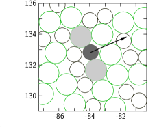
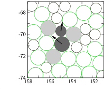
Figure 11: Configuration with fast particles, shown by dark gray. Panel (a) shows a particle with velocity $v/\left<v\right>\approx 8.5$. The reason for its high velocity is that it is squeezed between the two other particles, shown by light gray, and is therefore not in a force-balanced state. Panel (b) shows a configuration with two fast particles where a large net force on the big dark gray particle pushes on the small dark gray particle, which happens to be free to move and therefore also gets a high velocity.

Though a single unbalanced particle is the simplest case, the two dark gray particles in Fig. 11(b) also have high velocities. In this case a large net force on the big dark gray particle also makes the small dark gray particle move, and this kind of behavior may sometimes extend to chains of several particles. It should however be noted that a bigger number of particles give lower velocities for the same driving force. The tentative conclusion from this study is thus that the fast process is due to particles being squeezed, which is in contrast to getting their velocities by being pushed by other contacting particles with similar velocities.

A consequence of this picture is the presence of an additional time scale, related to the typical contact force, beside the time scale given by the shear strain rate. This is then a property which these particles have in common with avalanches that develop according to their intrinsic dynamics once they are set into motion.

It is interesting to note that two different times scales have previously been found in analyses of the auto-velocity correlation function Olsson (2010), where one of the time scales is directly related to the shear strain rate whereas the other is the “internal time scale”, $t_{\mathrm{int}}\sim 1/\sigma$. The conclusion that the dynamics of the fast particles in Fig. 11 is governed by a time scale related to the contact force, fits well together with $\sigma\sim\left<f_{ij}\right>$.

The examples discussed above are for the simple case of the fastest particles far out in the tail of the distribution, but it is less clear if it is possible to separate all particles into “fast” and “slow”, as would seem to be required by the splitting of the velocity distribution into two terms as in Eq. (19). One attempt in that direction would be to start from the picture that most particles—the slow ones—move around by being pushed by other particles with similar velocities and that the squeezing give rise to “fast” particles. One would however also need to characterize a particle as fast if it is pushed by another fast particle, but it is at present not clear if it is possible to device reasonable and useful criteria for such splitting into slow and fast particles. Another possibility would be to give up the idea of a strict splitting of particles into two disjunct categories, and instead say that any given particle may participate in, or be affected by, both the fast and the slow process.

III.7 Spatial velocity correlations

When the correlation length has been identified, one expects that the finite size dependence should be controlled by the dimensionless ratio $\xi/L$, where $L$ is the linear system size. In shear-driven jamming this does however not work out as expected. One example from the literature is in an attempted finite size scaling analysis at $\phi_{J}$ Vågberg et al. (2014b) where a decent collapse was found when data from different $L$ were plotted vs $L/\dot{\gamma}^{-1/z}$, with $z=6.5$, which is clearly different from the expected $z=1/0.26=3.85$. (As discussed in the jointly published Letter joi (2022) this difficulty is resolved by including a correction-to-scaling term. This finite size scaling does however work differently than commonly expected.) Another example that is difficult to reconcile with the expected behavior is a recent examination of the finite size dependence of data in a density range well below $\phi_{J}$, where the onset of finite size effects appeared at a constant $L$, even though the correlation length changes by more than a factor of two across the density interval in question Olsson (2022).

In critical phenomena one expects a direct link between the diverging correlation length and the diverging order parameter. As discussed above the shear viscosity is dominated by the fastest particles and we will now argue that the correlations are instead dominated by the slower particles, which is thus in contrast to this usual picture. To demonstrate that the correlations are dominated by slower particles we will use two sets of data, the “overlap function” and the velocity correlation function. The former has been widely used in the literature but the advantage of the latter is that it allows for a more direct interpretation in terms of the particle displacements.

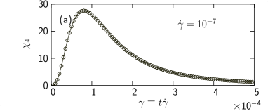
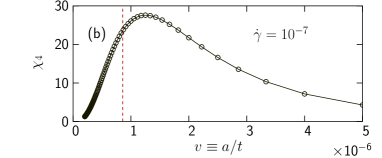
Figure 12: Dynamical susceptibility determined with probing length $a=0.001$. Panel (a) is $\chi_{4}$ vs $\gamma$ determined from the fluctuations in $Q_{1}(a,\gamma)$ which is, in turn, essentially the fraction of particles that have moved the distance $a$ during the shear $\gamma$. Panel (b) is the same data but plotted against $v=a/t\equiv a\dot{\gamma}/\gamma$, which is the average velocity needed for the particle to move the distance $a$ during a shear $\gamma$. We note that peak in $\chi_{4}$ is not far from the peak velocity $v_{p}$, shown by the dashed line.

To demonstrate that the velocity correlations are dominated by the slow particles we first examine the overlap function Lechenault et al. (2008); Heussinger et al. (2010) which for each individual configuration is determined from the positions of particles $i$ at a reference time $\mathbf{r}_{i}(0)$ and the positions at a time $t$ later, but compensated for the affine displacement, i.e. $\mathbf{r}_{i}(t)-\Delta_{i}(t)\hat{x}$. The overlap function is then

$$Q_{1}(a,t)=\frac{1}{N}\sum_{i=1}^{N}\exp\left(-\frac{|\mathbf{r}_{i}(t)-\Delta_{i}(t)\hat{x}-\mathbf{r}_{i}(0)|^{2}}{2a^{2}}\right),$$

where $a$ is a probing distance. The affine displacement, from the affine velocity field, $v_{x}=y\dot{\gamma}$, is given by $\Delta_{i}(t)=\int_{0}^{t}y_{i}(t^{\prime})\dot{\gamma}dt^{\prime}$. The dynamic susceptibility is Heussinger et al. (2010)

$$\chi_{4}(a,t)=N(\left<Q_{1}^{2}(a,t)\right>-\left<Q_{1}(a,t)\right>^{2}).$$ (26)

Fig. 12(a) shows $\chi_{4}$ vs $\gamma\equiv t\dot{\gamma}$. The peak in the plot shows the amount of shear at which half the particles have moved at least the probing length, $a=0.001$. We note that it is possible to extract a typical velocity from this, and determine the velocity from $v\equiv a/t$. These data are shown in Fig. 12(b) and lead to the conclusion that the collective dynamics is dominated by particles with $v_{4}\approx 1.25\times 10^{-6}$. We note that this velocity is not far from the peak velocity, $v_{p}=0.86\times 10^{-6}$, that characterizes the distribution of slow particles.

To show that most of the dissipation—and thus the dominant contribution to the shear stress— is due to particles with $v>v_{4}$, i.e. particles with considerably higher velocities than this characteristic velocity, we note that $S(v_{4})/\sigma$—the fraction of the dissipation due to particles with $v\leq v_{4}$—is small and decreases with decreasing shear strain rate. For $\dot{\gamma}=10^{-6}$, $10^{-7}$, and $10^{-8}$ the respective fractions are $S(v_{4})/\sigma\approx 0.051$, $0.044$, and $0.024$. The conclusion is thus that correlations and the contribution to the shear viscosity (i.e. dissipation) decouple in the $\dot{\gamma}\to 0$ limit as they are governed by different sets of particles.

A different way to reach the same conclusion is through analyses of the correlation function Olsson and Teitel (2020)

$$g(x)=\frac{\left<v_{x}(0)v_{x}(x\hat{x})\right>-\left<v_{y}(0)v_{y}(x\hat{x})\right>}{\mathbf{v}^{2}/2}.$$ (27)

In Ref. Olsson and Teitel (2020) it was concluded that $g(x)$ may be fitted to

$$g(x)=Ae^{-x/\xi}-Be^{-x/\ell},\quad A,B>0,$$ (28)

where the two terms describe the fluctuations in the rotation and the divergence of the velocity field. It was furthermore found that the diverging $\eta_{p}\equiv p/\dot{\gamma}$ scales with $\xi$, which thus suggests that it is $\xi$, which describes the decay of the rotations in the velocity field, that is the more significant correlation length, even though $\ell$ is often considerably bigger Olsson and Teitel (2020).

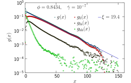
Figure 13: The splitting of the correlation function into three different terms. We here designate each particle as having “low” or “high” velocity with the threshold $v_{50}=5.46\times 10^{-6}$ chosen such that the sets of particles with low and high velocities each dissipate half the power. This is thus similar in spirit to the separation into slow and fast particles. Since each term that contributes to $g(x)$ involves two particles the full correlation function $g(x)$ may be split into three functions: $g_{\mathrm{ll}}(x)$ from two low velocity particles, $g_{\mathrm{lh}}(x)$ from one low velocity particle and one high velocity particle, and $g_{\mathrm{hh}}(x)$ from two high velocity particles. Since it is $g_{\mathrm{ll}}$ and (to a less extent) $g_{\mathrm{lh}}$ that dominate the correlations, the conclusion is that it is the low velocity particles that are behind the long range correlations in $g(x)$. The solid line is $\sim e^{-x/\xi}$ with $\xi=19.4$. The figure is for $N=65536$ particles, $\phi=0.8434$, and $\dot{\gamma}=10^{-7}$.

Since $g(x)$ gives clear evidence for long range velocity correlations it can be used to demonstrate that the correlations are dominated by the slower particles. To this end we define a threshold velocity $v_{50}$ such that half the power is dissipated by particles with low velocities, $v<v_{50}$ and half by the high velocity particles, $v>v_{50}$. We thus take $v_{50}$ to be the limit between low and high velocities, which is similar in spirit to “slow” and “fast” particles above, but with the difference that there is no sharp limit in the latter definition as the slow and the fast distributions overlap each other over a sizable velocity region. We then split $g(x)$ into terms $g_{\mathrm{ll}}(x)$, $g_{\mathrm{lh}}(x)$, and $g_{\mathrm{hh}}(x)$, which are the contributions to the correlation function from two low velocity particles, one particle with low velocity and one with high, and two high velocity particles, such that the full correlation function is $g(x)=g_{\mathrm{ll}}(x)+g_{\mathrm{lh}}(x)+g_{\mathrm{hh}}(x)$. These different terms, obtained at $\phi=0.8434\approx\phi_{J}$ and $\dot{\gamma}=10^{-7}$ with $v_{50}=5.46\times 10^{-6}$, are shown in Fig. 13.

The conclusion from this figure is that it is the low velocity particles that strongly dominate the correlations. The contributions from $g_{\mathrm{ll}}(x)$ is about 85%, from $g_{\mathrm{lh}}(x)$ the contribution is about 14%, and the contribution from $g_{\mathrm{hh}}(x)$—two high velocity particles—is less than 1% at large distances. In a sense this finding is not surprising since one can expect the build up of long range correlations in a system of elastic particles to be a slow process whereas the high velocities only exist for shorter times.

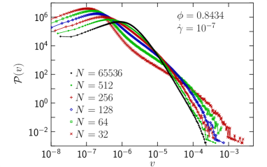
Figure 14: Finite size dependence of ${\cal P}(v)$ at $\phi=0.8434\approx\phi_{J}$ and $\dot{\gamma}=10^{-7}$. This figure shows that the low velocity region and the high velocity region are affected differently by a reduced system size such that the low-velocity peak moves to even lower velocities whereas the high-velocity tail extends to higher velocities.

The finding that slower particles contribute more to the velocity correlations than the faster particles leads to the expectation that a reduced system size should affect different parts of the velocity distribution differently. This expectation is borne out in Fig. 14 where it is found that the peak in the distribution moves to lower velocities as $N$ decreases whereas the tail moves in the opposite direction to higher velocities. An attempted explanation of the finite size dependence on the peak velocity is given in Sec. III.8, but we here present an explanation of the shift of the tail in the distribution to higher velocities. The reasonable explanation is that a reduced system size means a hindering of certain large-scale reorganizations that are needed for finding new low-energy configurations. When these large-scale reorganizations are no longer possible the system builds up bigger tensions, which are now and then reduced in more dramatic events with higher velocities, which leads to a shift of the tail of the velocity distribution to higher velocities.

III.8 Attempts to rationalize the findings

As an attempt to rationalize the findings we start by considering the slow process and turn to the fast process as a second step.

As a starting point we consider two contacting hard particles initially at rest at different $y$ coordinates, $\pm y/2$ and separation $d_{0}\mathbf{n}$ with the unit vector $\mathbf{n}=(n_{x},n_{y})$. Due to the homogeneous velocity profile these particles will experience opposite forces from this flow along the $x$ direction, $\pm(y/2)k_{d}\dot{\gamma}\hat{x}$, and also contact forces $f^{\mathrm{el}}_{\pm}$ in direction $\pm\mathbf{n}$. If there are no other interacting particles, the total velocities $v^{\mathrm{tot}}_{\pm}$ will be $v^{\mathrm{tot}}_{\pm}\mp y\dot{\gamma}\hat{x}=f^{\mathrm{el}}_{\pm}/k_{d}$, which together with $\mathbf{f}^{\mathrm{el}}\parallel\mathbf{n}$ and $\mathbf{v}^{\mathrm{tot}}\perp\mathbf{n}$ gives

$$n_{y}v^{\mathrm{tot}}_{\pm} = n_{x}f^{\mathrm{el}}/k_{d}\pm(y/2)\dot{\gamma},$$

$$n_{x}v^{\mathrm{tot}}_{\pm} = -n_{y}f^{\mathrm{el}}/k_{d},$$

and the relative particle velocity

$$v^{\mathrm{tot}}\equiv v^{\mathrm{tot}}_{+}-v^{\mathrm{tot}}_{-}=n_{y}y\;\dot{\gamma}.$$

In the presence of other particles that could hinder the displacement we expect this to instead lead to a force $k_{d}v^{\mathrm{tot}}$. Since the velocities at higher densities are correlated across a distance $\xi$ Olsson and Teitel (2020) it follows that any given contact should contribute a quantity $\propto\dot{\gamma}$ to the velocity field of each particle in the volume $\sim\xi^{2}$ centered at that contact.

We now instead turn to the behavior of a single particle and a consequence of the above discussion is that its velocity becomes affected by the $n=c_{\xi}^{2}\xi^{2}/d_{0}^{2}$ contacts in a volume $\xi^{2}$, where $c_{\xi}$ is a factor of order unity. We further assume that the relative velocity $v^{\mathrm{tot}}_{k}\sim d_{0}\dot{\gamma}$ at contact $k$ contributes $\bm{\eta}_{ik}d_{0}\dot{\gamma}$ to the velocity of particle $i$. For simplicity we take $\bm{\eta}_{ik}$ to be random and independent with $\left<\bm{\eta}_{ik}\right>=0$ and $\left<\bm{\eta}_{ik}^{2}\right>=c^{2}_{\eta}$. The velocity of a given particle then becomes $\mathbf{v}_{i}=\sum_{k=1}^{n}\bm{\eta}_{ik}d_{0}\dot{\gamma}$ where the sum is over the $n$ contacts with $\mathbf{r}_{ik}<\xi$. This gives $\left<\mathbf{v}_{i}\right>=0$, and the variance $\left<\mathbf{v}_{i}^{2}\right>=nc^{2}_{\eta}d_{0}^{2}\dot{\gamma}^{2}$ then defines a characteristic velocity

$$v^{\prime}=\sqrt{\left<\mathbf{v}_{i}^{2}\right>}=c_{\eta}\sqrt{n}d_{0}\dot{\gamma}=c\dot{\gamma}\xi,$$ (29)

where $c\equiv c_{\eta}c_{\xi}$ is a constant of order unity. For hard disks (or equivalently, soft disks at $\dot{\gamma}\to 0$) at densities below $\phi_{J}$ this becomes (cf. Eq. (4))

$$\eta^{\prime}_{\mathrm{hd}}=\frac{N}{V}k_{d}\frac{v^{\prime 2}}{\dot{\gamma}^{2}}=\frac{N}{V}k_{d}c^{2}\xi^{2}\sim\xi^{2},$$ (30)

and together with $\xi\sim(\phi_{J}-\phi)^{-1}$ Olsson and Teitel (2020) this leads to

$$\eta^{\prime}_{\mathrm{hd}}\sim(\phi_{J}-\phi)^{-2},$$ (31)

which is an estimate of the contribution from the slow particles, only, and not the full shear viscosity.

For an order of magnitude check we turn to low densities $\phi=0.78$ through 0.83 where the contribution from the slow particles should dominate the total $\eta$, determine $\xi$ as in Ref. Olsson and Teitel (2020) and make use of values of $\eta$ together with Eq. (30) to determine

$$c^{2}=\frac{\eta}{k_{d}(N/V)\xi^{2}}=0.8\pm 0.2.$$

which shows that $c$ is indeed a constant of order unity.

After this discussion of hard particles below jamming we turn to the behavior at $\phi_{J}$. We then make use of the correlation length $\xi\sim\dot{\gamma}^{-1/z}$, with $1/z=0.26$ Olsson and Teitel (2020). Eq. (29) then gives the characteristic velocity

$$v^{\prime}\sim\dot{\gamma}\;\dot{\gamma}^{-1/z}\sim\dot{\gamma}^{u^{\prime}},$$

with the exponent

$$u^{\prime}=1-1/z=0.74,$$

which is very close to $u_{v}=0.766$ for the peak velocity, $v_{p}\sim\dot{\gamma}^{u_{v}}$ in Eq. (16b). Though this agreement is encouraging as it suggests a connection between very different quantities, we note that the reasoning is still very incomplete as the behavior of $\xi$ is taken as a given starting point without any motivation.

Fig. 15(a) shows a direct comparison of $v_{p}$ and $v^{\prime}/c$ using $\xi\approx 0.29\dot{\gamma}^{-1/z}$ Olsson and Teitel (2020) in Eq. (29), and we note that they are very similar. The points $v^{\prime}/c$ are simply the values of $v^{\prime}$ when taking the unknown constant to be $c=1$.

[As a digression we now return to the behavior of hard particles below $\phi_{J}$ to compare our predictions based on $\sigma_{s}$ with Eq. (31). From the very similar behaviors of $v^{\prime}$ and $v_{p}$ one could expect an excellent agreement between predictions from $\sigma_{s}$ and Eq. (31), but there is instead a clear difference. For this discussion we make use of $\beta_{2}$, introduced in Sec. III.5, for the divergence of the secondary term. With $q_{2}=0.567$ and $z\nu=1/0.26$ $\beta_{2}=(1-q_{2})z\nu\approx 1.67$, is quite different from $\beta_{2}=2$ in Eq. (31). Recalling Eq. (18) and $q_{2}=u_{w}$ it turns out that one way to get $\beta_{2}=2$ is if the equalities $u_{v}=1-1/z\nu$ (this is $u_{v}=u^{\prime}$) and $u_{v}+u_{\cal P}=0$ were both fulfilled, but since they are only approximately fulfilled, the exponent instead becomes somewhat lower. It is interesting to note that $u_{v}+u_{\cal P}=0.033>0$ means that the fraction of particles with velocities up to the peak increases slowly with decreasing $\dot{\gamma}$. Such a trend is possible only because of the existence of two different processes.]

It is most interesting to also examine the dependence on system size. The starting point is then that a quantity which is determined from processes in a correlation volume should have a finite size dependence unless the linear system size is $L\gg\xi$. For small $L$ one expects $L$ to take the place of $\xi$, and Eq. (29) then becomes $v^{\prime}\sim\dot{\gamma}L$. Fig. 15, which shows $v_{p}$ vs $L$, gives evidence for such a behavior as the data below $L\approx 50$ follow the dashed line, $c^{\prime}\dot{\gamma}L$, to a good approximation. This is also the likely explanation of the size-dependence of $v_{p}$ in Fig. 14 which is $v_{p}\sim L$ for $N\leq 512$.

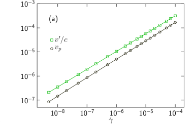
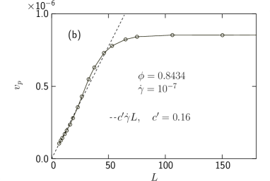
Figure 15: Attempts to test the rationalization of the shear rate dependence of the peak velocity in Eq. (29). Panel (a) shows a comparison between the peak velocity, $v_{p}$, and the characteristic velocity, from Eq. (29), shown as $v^{\prime}/c$; the data are encouragingly similar. (The open squares are the values of $v^{\prime}$, assuming $c=1$. Taking $v^{\prime}=v_{p}$ at $\dot{\gamma}=10^{-7}$ gives $c=0.45$.) Panel (b) shows the finite size effect on the peak velocity, $v_{p}$, by plotting $v_{p}$ vs $L$. The linear behavior $c^{\prime}\dot{\gamma}L$ with $c^{\prime}=0.16$, at small $L$, shown by the dashed line, is consistent with predictions in the main text. (The correlation length at $\phi\approx\phi_{J}$ and $\dot{\gamma}=10^{-7}$ is $\xi\approx 19$.)

Even though this picture describes the slow process, only, it also holds the seed to the fast process that gives particles with considerably higher velocities. We first recall that the condition for a wide tail in the velocity distribution is the presence of large contact forces, i.e. that the typical contact force is considerably larger than the typical net force $k_{d}v^{\prime}$ that drives the slow particles. The typical contact force, $f^{\prime}$, may be determined from the pressure which is given by $p^{\prime}=\sigma^{\prime}/\mu$, (where $\mu$ is the dimensionless friction). From $V/N\approx d_{0}^{2}$, $p^{\prime}\approx\frac{1}{4}f^{\prime}z/d_{0}$ and the approximate expressions for the contribution to the shear stress from the slow particles,

$$\sigma^{\prime}\approx\frac{N}{V}\frac{k_{d}}{\dot{\gamma}}v^{\prime 2},$$

and Eq. (29) one finds

$$f^{\prime}=\frac{N}{V}\frac{1}{\mu}\frac{k_{d}}{\dot{\gamma}}d_{0}v^{\prime 2}\approx\frac{c}{\mu}\frac{\xi}{d_{0}}k_{d}v^{\prime},$$ (32)

for the typical contact force. In most cases the contact forces on a particle almost cancel each other out, but in the case where the forces fail badly to balance each other out one finds

$$v_{\mathrm{fast}}=c_{g}f^{\prime}/k_{d}=\frac{c_{g}c}{\mu}\frac{\xi}{d_{0}}v^{\prime},$$ (33)

and even though the geometrical factor is $c_{g}\ll 1$, a big $\xi$ together with $1/\mu\approx 10$ (which holds close to jamming) may lead to velocities $v_{\mathrm{fast}}\gg v^{\prime}$. (That $c_{g}\ll 1$, is illustrated in Fig. 11(a) where the three particles are almost in a line and therefore give a resultant force that is considerably smaller than the contact forces.)

What finally gives the very high velocities, with tails extending up to $v\approx 100\;v_{p}$ for $\dot{\gamma}=10^{-7}$, is the fact that the above mentioned mechanism is self-amplifying since a number of fast particles have the effect to make $\left<v^{2}\right>>v^{\prime 2}$, which then increases $\sigma$ and the typical force, which in turn has the effect to increase $\left<v^{2}\right>$ even more.

IV Discussion

Short summary: The study of the velocity distribution in the present paper suggests the existence of two different processes with different scaling properties. We call them the slow process and the fast process as they are dominated by the slower particles in the peak and the faster particles in the tail of the distribution, respectively. Due to the relation between input power $\sigma\dot{\gamma}$ and dissipated power $k_{d}\left<v^{2}\right>$, Eq. (4), the shear stress is thought of as being controlled by the dissipation, which makes it possible to split the shear stress into contributions from the slow process and the fast process, $\sigma=\sigma_{s}+\sigma_{f}$. It is then found that the leading divergence of the shear viscosity is governed by the fast process whereas the correction-to-scaling term from the critical scaling analysis is related to the slow process. Since it is furthermore found that the long range velocity correlations that develop as criticality is approached, are due to the slow process, it appears that the connection expected in critical phenomena between the diverging correlation length and the diverging viscosity, is an indirect one, only. Taken together this suggests that shear-driven jamming is an unusual kind of critical phenomenon.

Open questions: There remain several open questions and one of them is on the mechanism behind the algebraic velocity distribution in the fast process. Since $v_{i}=f^{\mathrm{el}}_{i}/k_{d}$ the velocities, and thereby the velocity distribution, are directly given by the sum over the contact forces, $\mathbf{f}^{\mathrm{el}}_{i}=\sum_{j}\mathbf{f}^{\mathrm{el}}_{ij}$. The contact forces $\mathbf{f}^{\mathrm{el}}_{ij}$ are here from a narrow distribution whereas the distribution of the velocities (through the net forces) have a tail, $\sim v^{-r}$, with different $r$. An open question is what mechanism there is that generates this distribution.

A related enigmatic finding is that the values of $q$ and $q_{2}$ together give $q_{2}/q=1.995\pm 0.021$ (three standard deviations) which suggests the simple relation $q_{2}/q=2$. Though $q_{2}$ may be “understood” from the dependence of the velocity distribution on $\dot{\gamma}$, there is no simple way to come to grips with the exponent $q$ since it depends on both the exponent $r$, which changes with $\phi$ and $\dot{\gamma}$, and other properties of the tail of the distribution, in an opaque way. We here just speculate that there is a coupling between the two different processes that makes the system adjust itself to give this simple relation between the slow and the fast processes, but we have no clue to the underlying mechanism.

In critical phenomena the behavior is largely controlled by the main term, but in view of the present findings, that the diverging correlations appear to be present in the slow process, only, it could be that it is rather the slow process that is central in the critical phenomenon and, in some way, controls the fast process. If this is so it is perhaps more appropriate call $\sigma_{2}$ in Eq. (12) the “secondary term” rather than the correction-to-scaling term, as the latter term has the strong connotation of being small and insignificant.

Bucklers and the dimensionality: The fast particles in Fig. 11(a) are similar to the bucklers described in Ref. Charbonneau et al. (2015) which are found to be related to localized excitations. From that work it is also known that the population of bucklers decreases with higher dimensions and one could expect that this should also mean a lower frequency of fast particles and perhaps also that this separation into two different processes would no longer be relevant. We have however done some preliminary studies of the velocity histograms in both three and four dimensions and it is then clear that the picture described here remains essentially the same also in these higher dimensions. This could perhaps suggest that the processes as in Fig. 11(b), that give chains of fast particles, could be more important in higher dimensions.

Contact changes: Contact change events have been studied through quasistatic shearing of soft spheres and one has then found that these contact change events are of two different kinds where the first is irreversible and dramatic “rearrangements” that lead to discontinuous change of positions and the second is reversible and smooth “network events” Morse et al. (2020). The first kind has also been termed “jump changes” whereas the continuous contact change is termed a “point change” Tuckman et al. (2020). It does indeed seem that the fast and slow processes of the present work are respectively related to these different kinds of contact changes, and beside adding credibility to our picture of two different process, this connection also suggests new avenues for further research.

Relation to theoretically determined exponent: A further question is the connection between our findings and the theoretically determined value of the exponent $\beta/u_{z}$. The assumption that the process that governs the divergence of the shear viscosity is “spatially extended” DeGiuli et al. (2015) or “extensive” Ikeda (2020), is in contrast to our finding that the fast particles are short range correlated, only. Our finding could suggest going back to Ref. Lerner et al. (2012b) that presented a different results when using $\theta_{\ell}=0.18$ from the distribution of weak forces (determined for all contacts and not only the “extended” ones DeGiuli et al. (2015); Charbonneau et al. (2015)) and gave the value $\beta/u_{z}=(3+\theta_{\ell})/(1+\theta_{\ell})=2.69$ in excellent agreement with the simulations in 2D Olsson (2015). In spite of this agreement in 2D (which could perhaps be just fortuitous) a remaining question is the reason for the different exponent in three dimensions, and we conclude that more work is needed to sort out this question.

Future and ongoing work: There are quite a few interesting directions for the further research. As already mentioned a finite size scaling study of shear-driven jamming, by means of the splitting into $\sigma_{s}$ and $\sigma_{f}$, is under way. We then also plan to examine models with elliptical and ellipsoidal particles, and/or with different models for dissipation, with the key question what properties of the model that determine the universality class of the transition. It would also be interesting to examine how the introduction of inertia—which is known to give an altogether different behavior Trulsson et al. (2012)—is reflected in the properties of the velocity distribution.

Appendix A Determination of $\phi_{J}$ and the exponents $q$ and $q_{2}$

To determine the exponents with the highest possible precision we simultaneously fit shear stress to Eq. (12) and pressure to Eq. (13). We are then inspired by Ref. Rahbari et al. (2018) who use the same exponents $q$ for both quantities and $q^{(p)}_{2}=q_{2}$. That $q$ should be the same for both quantities follows from the understanding that $\mu\equiv\sigma/p$ approaches a constant at jamming, whereas the same value of the exponent for the second term for both quantities follows from the correction-to-scaling exponent being the same for different quantities. Just in order to examine all possibilities we have however also examined the possibility that the secondary exponents could be different, and in Table 1 we therefore show results from a few different kinds of fits. Method (A) is from fitting $\sigma$ only, method (B) is from a simultaneous fit of $\sigma$ and $p$ where we take $q$ to be the same for both $\sigma$ and $p$ but let $q_{2}$ and $q^{(p)}_{2}$ be different fitting parameters. Since the correction term is considerably smaller for $p$ than for $\sigma$, the main effect of including data for $p$ is to get better precision in $q$ which in turn gives a smaller error in $q_{2}$. In method (C) we demand $q^{(p)}_{2}=q_{2}$ which gives slightly lower values of both $q$ and $q_{2}$. The simultaneous fitting of $\sigma$ and $p$ gives a very sensitive method and Fig. 16 shows how the quality of the fit depends on the assumed $\phi_{J}$. The optimal fit is obtained with $\phi_{J}=0.843~{}43$, just slightly higher than $\phi_{J}\approx 0.8434$ used throughout this paper. We also note that the values are in good agreement with Ref. Olsson and Teitel (2011) that gave $\phi_{J}=0.843~{}47$, $q=0.28(2)$, and that our $q_{2}-q=0.285(5)$ is in good agreement with $\omega/\nu=0.29(3)$ Olsson and Teitel (2011). Just as in Ref. Rahbari et al. (2018) it is the combination of two sets of data that narrows down the possible values of $\phi_{J}$ to a very small interval in $\phi$.

method	$\phi_{J}$	$q$	$q_{2}$	remark
A	0.8434	0.29(2)	0.58(5)	fitting $\sigma$, only,
B	0.8434	0.290(2)	0.58(1)	$q^{(p)}_{2}=1.1(5)$
C	0.8434	0.284(2)	0.567(7)	demanding $q^{(p)}_{2}=q_{2}$
C	0.84343	0.281(3)	0.567(8)	at $\phi_{J}$ from Fig. 16.

Table 1: Four different determinations of the exponents $q$ and $q_{2}$. Method A which is from using $\sigma(\phi=0.8434,\dot{\gamma})$ only gives rather poor precision in the exponents. In method B we make use of $p(\phi=0.8434,\dot{\gamma})$ to give higher precision in $q$, but keeping $q^{(p)}_{2}$ as a separate fitting parameter from $q_{2}$. In method C we demand $q^{(p)}_{2}=q_{2}$, but still assume $\phi_{J}=0.8434$. The last line is from a fit with method C but assuming different jamming densities $\phi_{J}=0.843~{}40$ through 0.843 48. From the quality of the fit, shown in Fig. 16, we then determine $\phi_{J}=0.843~{}43$ which is our value of $\phi_{J}$. In this determination the $\sigma(\phi,\dot{\gamma})$ are obtained by interpolating $\sigma(\phi,\dot{\gamma})$ measured at $\phi=0.8434$ and 0.8435.

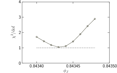
Figure 16: Determination of the jamming density. The figure shows the quality of the fits in terms of $\chi^{2}/\mathrm{dof}$ when assuming different values of $\phi_{J}$ and using method C, i.e. demanding that both $q$ and $q_{2}$ should be the same in the fit of $\sigma(\phi,\dot{\gamma})$ to Eq. (12) and in the fit of $p(\phi,\dot{\gamma})$ to Eq. (13). The value $\phi_{J}\approx 0.843~{}43$ obtained here was used in the determination of $I_{2}$ shown in Fig. 5, since that determination is very sensitive to the value of $\phi_{J}$; we have otherwise used $\phi_{J}\approx 0.8434$ throughout the paper.

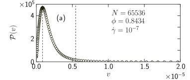
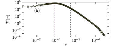
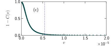
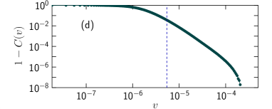
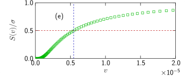
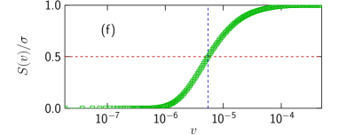
Figure 17: Velocity distribution and relative dissipation at $\phi\approx\phi_{J}$ and $\dot{\gamma}=10^{-7}$. Panel (a) shows ${\cal P}(v)$ on linear scales (which simplifies the understanding of the distributions) whereas panel (b) shows the same data (though extending to higher $v$) on a double-log scale. Panels (c) and (d) are $1-C(v)$ which is the fraction of particles with velocity $>v$. Panels (e) and (f) show $S(v)$ from the cumulative dissipation with the vertical dashed line marking $v_{50}$ which is at 50% of the dissipation. It is clear that a fair part of the dissipation is from particles with velocities far out in the tail of the distribution.

Appendix B Velocity distribution on linear and logarithmic scales

As jamming is approached the velocity distribution develops a wide tail and it then becomes convenient to plot data on a double-log scale. The obvious drawback is that the figures then become difficult to interpret and we therefore show a typical example of ${\cal P}(v)$ —here obtained at $\phi=0.8434\approx\phi_{J}$ and $\dot{\gamma}=10^{-7}$—in Fig. 17(a) and (b) plotted in two different ways with linear and logarithmic scales. Fig. 17(a) shows that ${\cal P}(v)$ has a peak at the low velocity $v_{p}\approx 8.6\times 10^{-7}$ and from Fig. 17(b), which is the same data (though extending to higher $v$) on a double-log scale, it is clear that the distribution extends up to much larger velocities, even above $100\;v_{p}$. Fig. 17(c) and (d) show $1-C(v)$, which is the fraction of particles with velocity $>v$. Here $C(v)=\int_{0}^{v}{\cal P}(v^{\prime})dv^{\prime}$ is the cumulative velocity distribution.

Fig. 17(e) and (f) show the relative contribution to the shear viscosity for particles with nonaffine velocity $<v$, obtained as $S(v)/\sigma$, and it is clear that a fair part of the dissipation is from velocities far out in the tail of the distribution. From the figure it follows that more than 25% of the dissipation is for $v>10^{-5}$ even though it could seem from Fig. 17(a) that ${\cal P}(v)$ is negligible in that region and the same figure gives at hand that 50% of the energy is dissipated by only about 3.6% of the fastest particles. This is, furthermore, a fraction that keeps decreasing as $\dot{\gamma}\to 0$.

Appendix C On the origin of the wide velocity distribution

A possible view on the anomalously large velocities that make up the tail of the velocity distribution is that they occur when, due to a fluctuation, the critical volume fraction for a particular configuration is anomalously small, so that the large velocities actually reflect the elasto-plastic type behavior of a jammed configuration, rather than the behavior of a packing of hard particles at constant pressure, below jamming.

That kind of picture is a natural one when approaching the subject from the analysis of static packings. Quite a few things are however different in shear-driven simulations close to $\phi_{J}$ and one of these is that it is not obvious that $p$ may be used to tell about the “true distance to jamming”, when the shearing systems are very far from equilibrium.

In shear-driven jamming at low shear strain rates and well below the jamming density $\phi_{J}\approx 0.8434$, say $\dot{\gamma}=10^{-7}$ and $\phi=0.83$, things are simple. When stopping the shearing and relaxing a configuration to a zero-energy state, the contact number $z$ of the zero-energy state, is strongly correlated to $p$ of the initial configuration. If one then tried to determine $\phi_{c}$ by compressing the relaxed configuration further, one would presumably also find this $\phi_{c}$ to be strongly correlated to $p$ of the initial configuration.

Closer to $\phi_{J}$—which is the region for most of our simulations—the correlation between $p$ and $z$, however, becomes much smaller and the obvious reason is that the relaxations often require substantial reorganizations and during these reorganizations the system loses memory of it original state. A consequence is that we can no longer expect $p$ to determine $\phi_{c}$.

It should also be noted that the fluctuations of $p$ are quite small. For $N=65536$ particles at $\phi=0.8434\approx\phi_{J}$, and shear strain rate $\dot{\gamma}=10^{-7}$ the standard deviation of $p$ is, in relative terms, $\mathrm{std}(p)/p\approx 0.05$ and this is by itself evidence that the fluctuations in $p$ cannot be the reason for the wide velocity distribution.

References

- O’Hern et al. (2003) C. S. O’Hern, L. E. Silbert, A. J. Liu, and S. R. Nagel, Phys. Rev. E 68, 011306 (2003).
- Durian (1995) D. J. Durian, Phys. Rev. Lett. 75, 4780 (1995).
- Alexander (1998) S. Alexander, Physics Reports 296, 65 (1998).
- Goodrich et al. (2012) C. P. Goodrich, A. J. Liu, and S. R. Nagel, Phys. Rev. Lett. 109, 095704 (2012).
- Charbonneau et al. (2014a) P. Charbonneau, J. Kurchan, G. Parisi, P. Urbani, and F. Zamponi, Nature Communications 5, 3725 (2014a).
- Charbonneau et al. (2014b) P. Charbonneau, J. Kurchan, G. Parisi, P. Urbani, and F. Zamponi, Journal of Statistical Mechanics: Theory and Experiment 2014, P10009 (2014b).
- Charbonneau et al. (2015) P. Charbonneau, E. I. Corwin, G. Parisi, and F. Zamponi, Phys. Rev. Lett. 114, 125504 (2015).
- DeGiuli et al. (2015) E. DeGiuli, G. Düring, E. Lerner, and M. Wyart, Phys. Rev. E 91, 062206 (2015).
- Ikeda (2020) H. Ikeda, J. Chem. Phys. 153, 126102 (2020).
- Lerner et al. (2012a) E. Lerner, G. Düring, and M. Wyart, PNAS 109, 4798 (2012a).
- Olsson (2015) P. Olsson, Phys. Rev. E 91, 062209 (2015).
- Olsson (2019) P. Olsson, Phys. Rev. Lett. 122, 108003 (2019).
- Nishikawa et al. (2021) Y. Nishikawa, A. Ikeda, and L. Berthier, J. Stat. Phys. 182, 37 (2021).
- Olsson (2022) P. Olsson, Phys. Rev. E 105, 034902 (2022).
- Andreotti et al. (2012) B. Andreotti, J.-L. Barrat, and C. Heussinger, Phys. Rev. Lett. 109, 105901 (2012).
- Olsson and Teitel (2011) P. Olsson and S. Teitel, Phys. Rev. E 83, 030302(R) (2011).
- Kawasaki et al. (2015) T. Kawasaki, D. Coslovich, A. Ikeda, and L. Berthier, Phys. Rev. E 91, 012203 (2015).
- Heussinger and Barrat (2009) C. Heussinger and J.-L. Barrat, Phys. Rev. Lett. 102, 218303 (2009).
- Wyart et al. (2005) M. Wyart, L. E. Silbert, S. R. Nagel, and T. A. Witten, Phys. Rev. E 72, 051306 (2005).
- Pouliquen (2004) O. Pouliquen, Phys. Rev. Lett. 93, 248001 (2004).
- Lechenault et al. (2008) F. Lechenault, O. Dauchot, G. Biroli, and J. P. Bouchaud, Europhys. Lett. 83, 46003 (2008).
- Heussinger et al. (2010) C. Heussinger, L. Berthier, and J.-L. Barrat, Europhys. Lett. 90, 20005 (2010).
- Olsson and Teitel (2020) P. Olsson and S. Teitel, Phys. Rev. E 102, 042906 (2020).
- Olsson (2016) P. Olsson, Phys. Rev. E 93, 042614 (2016).
- joi (2022) (2022), see the related paper in Physical Review Letters, P. Olsson.
- Evans and Morriss (1990) D. J. Evans and G. P. Morriss, Statistical Mechanics of Nonequilibrium Liquids (Academic Press, London, 1990).
- Vågberg et al. (2014a) D. Vågberg, P. Olsson, and S. Teitel, Phys. Rev. Lett. 112, 208303 (2014a).
- Ono et al. (2003) I. K. Ono, S. Tewari, S. A. Langer, and A. J. Liu, Phys. Rev. E 67, 061503 (2003).
- Olsson and Teitel (2007) P. Olsson and S. Teitel, Phys. Rev. Lett. 99, 178001 (2007).
- Vågberg et al. (2016) D. Vågberg, P. Olsson, and S. Teitel, Phys. Rev. E 93, 052902 (2016).
- Rahbari et al. (2018) S. H. E. Rahbari, J. Vollmer, and H. Park, Phys. Rev. E 98, 052905 (2018).
- Olsson (2010) P. Olsson, Phys. Rev. E 81, 040301(R) (2010).
- Vågberg et al. (2014b) D. Vågberg, P. Olsson, and S. Teitel, Phys. Rev. Lett. 113, 148002 (2014b).
- Morse et al. (2020) P. Morse, S. Wijtmans, M. van Deen, M. van Hecke, and M. L. Manning, Phys. Rev. Res. 2, 023179 (2020).
- Tuckman et al. (2020) P. J. Tuckman, K. VanderWerf, Y. Yuan, S. Zhang, J. Zhang, M. D. Shattuck, and C. S. O’Hern, Soft Matter 16, 9443 (2020).
- Lerner et al. (2012b) E. Lerner, G. Düring, and M. Wyart, Europhys. Lett. 99, 58003 (2012b).
- Trulsson et al. (2012) M. Trulsson, B. Andreotti, and P. Claudin, Phys. Rev. Lett. 109, 118305 (2012).