A long-period pre-ELM system discovered from LAMOST medium-resolution survey

Abstract

We present LAMOST J041920.07+072545.4 (hereafter J0419), a close binary consisting of a bloated extremely low mass pre-white dwarf (pre-ELM WD) and a compact object with an orbital period of 0.607189 days. The large-amplitude ellipsoidal variations and the evident Balmer and He I emission lines suggest a filled Roche lobe and ongoing mass transfer. No outburst events were detected in the 15 years of monitoring of J0419, indicating a very low mass transfer rate. The temperature of the pre-ELM, $T_{\mathrm{eff}}=5793_{-133}^{+124}\,\rm K$, is cooler than the known ELMs, but hotter than most CV donors. Combining the mean density within the Roche lobe and the radius constrained from our SED fitting, we obtain the mass of the pre-ELM, $M_{1}=0.176\pm 0.014\,M_{\odot}$. The joint fitting of light and radial velocity curves yields an inclination angle of $i=66.5_{-1.7}^{+1.4}$ degrees, corresponding to the compact object mass of $M_{2}=1.09\pm 0.05\,M_{\odot}$. The very bloated pre-ELM has a smaller surface gravity ($\log g=3.9\pm 0.01$, $R_{1}=0.78\pm 0.02\,R_{\odot}$) than the known ELMs or pre-ELMs. The temperature and the luminosity ($L_{\mathrm{bol}}=0.62_{-0.10}^{+0.11}\,L_{\odot}$) of J0419 are close to the main sequence, which makes the selection of such systems through the HR diagram inefficient. Based on the evolutionary model, the relatively long period and small $\log g$ indicate that J0419 could be close to the “bifurcation period” in the orbit evolution, which makes J0419 to be a unique source to connect ELM/pre-ELM WD systems, wide binaries and cataclysmic variables.

1 Introduction

Extremely low mass white dwarfs (ELM WDs) are helium-core WDs with masses below $0.3\,M_{\odot}$ (Li et al., 2019), which are different from most WDs that have C/O cores with mass around $0.6\,M_{\odot}$ (Kepler et al., 2015). ELM WDs are thought to be born in interactive binaries and have lost most of their mass to the companions through either the stable Roche lobe overflow or the common-envelope evolution (CE), as the formation time of a WD with mass less than 0.3 $M_{\odot}$ produced from a single star exceeds the Hubble timescale. Chen et al. (2017); Sun & Arras (2018); Li et al. (2019) theoretical studied the formation of ELMs and showed that the progenitors of ELMs fill the Roche lobes at the end of the main sequence (MS) or near the base of the red giant branch (RGB). When the mass transfer ceases, possibly due to the stop of the magnetic braking driven orbital contraction (see Sun & Arras, 2018; Li et al., 2019), a pre-ELM with a helium core and a hydrogen envelope is formed. In this paper, we use pre-ELMs to refer to all progenitors of ELMs. After the detachment of the binary, the envelope will continue burning to keep a nearly constant luminosity until the burnable hydrogen is exhausted, and the radius of the envelope will gradually shrink. The hydrogen exhausted pre-ELM will enter the WD cooling track.

The research of ELMs/pre-ELMs has gradually become active in recent years. Many pre-ELMs or ELMs have pulsations (Maxted et al., 2011, 2013, 2014a; Gianninas et al., 2016; Zhang et al., 2017), which provide unprecedented opportunities to explore their interiors. The high accretion rate in the early stages of the ELM formation may contribute enough mass to the C/O WD companion in the binary and makes it a progenitor of a Type Ia supernova (Han & Podsiadlowski, 2004). The compact ELMs, such as J0651+2844, that has a period of 765 s (Brown et al., 2011; Amaro-Seoane et al., 2012), could be resolved by future space-based gravitational-wave detectors (Amaro-Seoane et al., 2012; Luo et al., 2016b).

More than 100 ELM WDs and their progenitors have been reported by several surveys, e.g., the Kepler project (van Kerkwijk et al., 2010; Carter et al., 2011; Breton et al., 2012; Rappaport et al., 2015), the WASP project (Maxted et al., 2011, 2013, 2014a, 2014b), the ELM survey (Brown et al., 2010, 2012, 2013, 2016, 2020; Kilic et al., 2011, 2012, 2015; Gianninas et al., 2014, 2015), and the ELM survey South (Kosakowski et al., 2020). Most of the objects reported by previous works are ELMs in double degenerates (DD) binaries, and their companions are WDs (Li et al., 2019) or neutron stars (Istrate et al., 2014a, b). Some works reported the pre-ELMs in EL CVn-type binaries, which are post-mass transfer eclipsing binaries that are composed of an A/F-type main sequence star and a progenitor of ELM in the shrinking stage (Maxted et al., 2011, 2014a; Wang et al., 2018, 2020). All of these sources have ended their mass interactions.

The pre-ELMs in mass transfer or terminated mass transfer recently have temperatures similar to the main sequence A and F stars and can not be selected by their colors. By inspecting light curves with large amplitude ellipsoidal variability and luminosities below the main sequence, El-Badry et al. (2021a, b) reported a sample of pre-ELMs in DDs with periods less than 6 hours. They name these sources proto-ELMs. The objects of El-Badry et al. (2021a, b) have lower temperatures than ELMs and the pre-ELMs in EL CVns. Moreover, their objects with temperatures lower than 6500 K have emission lines, and the rest objects with higher temperatures do not have, indicating that the sample of El-Badry et al. (2021a, b) are in the transition from mass transfer to detached.

The pre-ELM WDs with stable mass transfer behave as cataclysmic variables (CVs). Unlike normal CVs, pre-ELMs are evolved stars with Helium-cores. They have much lower mass transfer rates than normal CVs, and do not show typical CV characteristics in the light curves, such as random variation in a short timescale, outburst events. Normal CVs generally have small-mass donors in the main sequence whose orbital periods are several hours (Knigge, 2006; Knigge et al., 2011). The stellar parameters, such as mass, radius, spectral type, and luminosity, are closely related to the orbital period, which is called “donor sequence” (Patterson, 1984; Beuermann et al., 1998; Smith & Dhillon, 1998; Knigge, 2006; Knigge et al., 2011). With bloated radius and helium cores, the evolved donors significantly deviate from the donor sequence. They have smaller mass and higher temperatures compared with the donor in normal CVs (Podsiadlowski et al., 2003; van der Sluys et al., 2005; Kalomeni et al., 2016).

The evolution trace of the ELMs mainly depends upon the initial period and initial mass (Li et al., 2019). The donors with longer initial periods will be more evolved before the mass transfer, resulting in pre-ELMs with more bloated radii and longer periods. These long-period pre-ELMs are close to the main sequence and, therefore, cannot be selected using the HR diagram. Meanwhile, some long-period pre-ELMs may have periods close to the bifurcation period. Theoretically speaking, for the systems with orbital periods longer than the bifurcation period (16–22 h), the donors ascend the giant branch as the mass transfer begins, and the systems evolve toward long orbital periods with mass loss (Podsiadlowski et al., 2003). For the systems whose period is shorter than the bifurcation period, the orbits of these targets are contracting rather than expanding because of magnetic braking. The pre-ELMs with periods close to the bifurcation period are special cases between these two situations and vital for our understanding of the evolution of ELM systems.

In this work, we report the discovery of a pre-ELM with a period of 14.6 hours, which is much longer than typical pre-ELMs. The orbital period of this source is about three times that of the sample in El-Badry et al. (2021a), so the surface gravity is less than that of all ELMs or pre-ELMs we have known. Because of the larger radius and higher luminosity, this object almost falls on the main sequence, making it inefficient to select this type of object using the HR diagram. Thanks to the time-domain spectroscopic (e.g., the Large Sky Area Multi-Object Fiber Spectroscopic Telescope; LAMOST; see Cui et al. 2012; Zhao et al. 2012) and photometric surveys, we are able to select such a particular pre-ELM.

The paper is organized as follows. In Section 2, we describe the data, which include the spectroscopic data from several telescopes or instruments, and the photometric data from publicly available photometric surveys. In Section 3, we present the process of data measurement and analysis, including determination of orbital period, radial-velocity (RV) measurements, SED fitting, and spectral matching. Discussion and summary are made in Sections 4 and 5.

2 Data

J0419 (R.A. = $04^{h}19^{m}20^{s}.07$, Decl. = $07\degree 25^{\prime}45^{\prime\prime}.4$, J2000) is selected from the LAMOST medium-resolution surveys (MRS; Liu et al., 2020) and has a stellar type of G8 and a magnitude of 14.70 mag in the Gaia $G$-band. The RV measurements of LAMOST DR8 MRS show that this source has an RV variation of about 212 $\mathrm{km\,s^{-1}}$ by six exposures on Nov 8, 2019. Since the absorption lines of the LAMOST spectra are single-lined, we speculate J0419 is a binary composed of a visible star and a compact object. We applied for additional spectroscopic observations to constrain the RV amplitude of J0419 by using the 2.16-meter telescope in Xinglong and the Lijiang 2.4-meter telescope. We also requested several LAMOST follow-up observations on this source. The observation information is summarized in Table 1. In addition to spectroscopic data, we collected photometric data from several publicly available sky surveys, which include the Transiting Exoplanet Survey Satellite (TESS; Ricker et al., 2015), the Catalina Real-time Transient Survey (CRTS; Drake et al., 2009, 2014), the All-Sky Automated Survey for Supernovae (ASAS-SN Shappee et al., 2014; Kochanek et al., 2017) and the Zwicky Transient Facility (ZTF; Masci et al., 2019). The data are described below.

Table 1: Statistics of the observed spectra of J0419

Num	Telescope	HMJD	Obs. Date	Exp. time (s)	Phase	SNR	Resolution	RV ($\mathrm{km\,s^{-1}}$)	$\rm EW_{H\alpha}$ (Å)
1	LAMOST MRS	58795.69	2019-11-08 16:36:34	1200	0.93	10.1	7500	$166.3_{-5.8}^{+5.8}$	$4.03\pm 0.17$
2	LAMOST MRS	58795.71	2019-11-08 16:59:34	1200	0.96	9.2	7500	$129.7_{-4.8}^{+6.8}$	$3.41\pm 0.18$
3	LAMOST MRS	58795.72	2019-11-08 17:22:34	1200	0.99	8.4	7500	$97.2_{-7.5}^{+5.8}$	$4.12\pm 0.20$
4	LAMOST MRS	58795.76	2019-11-08 18:12:34	1200	0.04	10.7	7500	$17.5_{-5.8}^{+5.5}$	$4.36\pm 0.15$
5	LAMOST MRS	58795.78	2019-11-08 18:36:34	1200	0.07	10.1	7500	$-13.3_{-4.0}^{+4.0}$	$4.22\pm 0.17$
6	LAMOST MRS	58795.79	2019-11-08 18:59:34	1200	0.10	10.3	7500	$-45.8_{-4.8}^{+5.5}$	$3.94\pm 0.17$
7	LAMOST LRS	58837.61	2019-12-20 14:42:16	600	0.97	20.6	1800	$104.5_{-7.0}^{+6.0}$	$10.10\pm 0.17$
8	LAMOST LRS	58837.62	2019-12-20 14:56:16	600	0.99	20.2	1800	$90.5_{-8.0}^{+7.0}$	$9.05\pm 0.17$
9	LAMOST LRS	58837.63	2019-12-20 15:09:16	600	0.00	21.5	1800	$65.8_{-7.0}^{+7.0}$	$8.43\pm 0.16$
10	LAMOST LRS	58837.65	2019-12-20 15:31:16	600	0.03	23.5	1800	$30.0_{-6.0}^{+6.0}$	$9.59\pm 0.16$
11	LAMOST LRS	58837.66	2019-12-20 15:45:16	600	0.05	25.2	1800	$9.3_{-6.0}^{+6.0}$	$9.14\pm 0.15$
12	LAMOST LRS	58837.67	2019-12-20 15:58:16	600	0.06	26.3	1800	$-12.8_{-6.8}^{+6.0}$	$9.73\pm 0.14$
13	2.16-meter	59140.74	2020-10-18 17:39:32	1800	0.20	119.0	300	-	$15.69\pm 0.12$
14	2.16-meter	59140.76	2020-10-18 18:09:37	1800	0.23	107.7	300	-	$15.64\pm 0.11$
15	2.16-meter	59140.79	2020-10-18 18:56:15	1800	0.28	107.2	300	-	$16.03\pm 0.11$
16	2.16-meter	59140.81	2020-10-18 19:26:20	1800	0.32	102.4	300	-	$16.65\pm 0.11$
17	2.16-meter	59140.83	2020-10-18 19:57:45	1200	0.35	80.3	300	-	$16.22\pm 0.13$
18	2.16-meter	59140.85	2020-10-18 20:17:50	1200	0.38	73.4	300	-	$16.45\pm 0.14$
19	2.16-meter	59140.86	2020-10-18 20:37:55	1200	0.40	70.9	300	-	$17.03\pm 0.14$
20	2.16-meter	59141.75	2020-10-19 17:56:03	1200	0.86	68.7	300	-	$14.09\pm 0.17$
21	2.16-meter	59141.76	2020-10-19 18:16:08	1200	0.88	67.7	300	-	$13.36\pm 0.18$
22	2.16-meter	59141.78	2020-10-19 18:36:13	1200	0.91	64.9	300	-	$13.05\pm 0.18$
23	2.16-meter	59141.80	2020-10-19 19:09:25	1200	0.95	64.1	300	-	$12.07\pm 0.18$
24	2.16-meter	59141.81	2020-10-19 19:29:30	1200	0.97	65.3	300	-	$12.39\pm 0.17$
25	2.16-meter	59141.83	2020-10-19 19:49:35	1200	0.99	63.3	300	-	$14.59\pm 0.17$
26	2.16-meter	59141.84	2020-10-19 20:10:01	1200	0.02	61.1	300	-	$14.35\pm 0.19$
27	2.16-meter	59141.85	2020-10-19 20:30:06	1200	0.04	61.2	300	-	$15.92\pm 0.18$
28	2.16-meter	59141.87	2020-10-19 20:50:11	1200	0.06	57.7	300	-	$14.97\pm 0.17$
29	2.16-meter	59192.62	2020-12-09 14:46:53	1800	0.64	47.4	620	$232.5_{-24.0}^{+12.8}$	$8.27\pm 0.20$
30	2.16-meter	59192.64	2020-12-09 15:16:59	1800	0.67	48.9	620	$284.2_{-24.0}^{+13.0}$	$9.31\pm 0.21$
31	2.16-meter	59192.66	2020-12-09 15:57:02	1800	0.72	56.1	620	$318.7_{-19.8}^{+5.9}$	$9.63\pm 0.17$
32	2.16-meter	59192.69	2020-12-09 16:27:08	1800	0.75	56.3	620	$303.0_{-21.2}^{+6.5}$	$9.85\pm 0.17$
33	2.16-meter	59192.71	2020-12-09 17:06:44	1800	0.80	55.7	620	$278.8_{-21.9}^{+6.1}$	$8.57\pm 0.17$
34	2.16-meter	59192.74	2020-12-09 17:40:42	1800	0.84	53.2	620	$265.1_{-22.3}^{+6.4}$	$7.94\pm 0.19$
35	LAMOST MRS	59213.57	2020-12-30 13:37:59	1200	0.15	3.4	7500	$-74.7_{-23.2}^{+21.2}$	$4.83\pm 0.76$
36	LAMOST MRS	59213.58	2020-12-30 14:01:23	1200	0.17	3.5	7500	$-66.6_{-21.2}^{+21.2}$	$8.03\pm 1.10$
37	LAMOST MRS	59213.60	2020-12-30 14:24:45	1200	0.20	3.6	7500	$-111.0_{-14.2}^{+14.1}$	$11.95\pm 0.92$
38	LAMOST MRS	59213.62	2020-12-30 14:48:09	1200	0.23	3.7	7500	$-118.1_{-18.1}^{+13.2}$	$12.73\pm 0.75$
39	LAMOST MRS	59213.64	2020-12-30 15:18:54	1200	0.26	3.2	7500	$-108.9_{-20.3}^{+27.2}$	$13.20\pm 0.88$
40	LAMOST MRS	59213.65	2020-12-30 15:42:17	1200	0.29	3.1	7500	$-112.0_{-67.6}^{+29.3}$	-
41	LAMOST MRS	59240.47	2021-01-26 11:13:44	1200	0.45	2.0	7500	$7.0_{-18.3}^{+21.8}$	$-0.19\pm 0.96$
42	LAMOST MRS	59240.48	2021-01-26 11:37:44	1200	0.48	2.6	7500	$27.0_{-20.0}^{+24.8}$	$1.40\pm 0.83$
43	LAMOST MRS	59240.50	2021-01-26 12:00:44	1200	0.50	2.6	7500	$98.7_{-56.1}^{+23.5}$	$-0.22\pm 0.83$
44	LAMOST MRS	59242.47	2021-01-28 11:11:18	1200	0.74	5.8	7500	$307.5_{-9.1}^{+10.0}$	$9.03\pm 0.60$
45	LAMOST MRS	59242.48	2021-01-28 11:34:40	1200	0.77	4.8	7500	$305.4_{-24.1}^{+23.2}$	$8.13\pm 0.59$
46	LAMOST MRS	59242.50	2021-01-28 11:58:02	1200	0.79	5.0	7500	$301.4_{-16.1}^{+13.1}$	$5.88\pm 0.58$
47	Lijiang 2.4-meter	59248.55	2021-02-03 13:09:16	1801	0.76	40.5	850	$299.7_{-12.0}^{+13.0}$	$2.67\pm 0.18$

Note. — The HMJD is the mid-exposure time. The heliocentric corrections have been applied to the RVs. We did not measure the RVs of the spectra observed by using the G4 grism due to their low resolution. The spectrum of line 40 has no red arm data and therefore no information about the $\rm H\alpha$ emission line.

2.1 Spectroscopic Data

2.1.1 LAMOST spectra

LAMOST is a uniquely designed 4-meter reflecting Schmidt telescope that enables it to observe 4000 spectra simultaneously in a field of view of $5^{\circ}$ (Cui et al., 2012; Zhao et al., 2012). The wavelength coverage of LAMOST low-resolution ($R\sim 1800$) spectra ranges from 3690 Å to 9100 Å (Luo et al., 2016a). The LAMOST medium-resolution ($R\sim 7500$; see Liu et al. 2020) spectra have two arms, of which the blue arm covers the wavelength range of 4950 Å to 5350 Å, and the red arm covers a wavelength range of 6300 Å to 6800 Å (Zong et al., 2018). For both low- and medium-resolution spectra, the LAMOST’s observation strategy is to perform 2–4 consecutive short exposures for 10–20 minutes each (see Table 1). In the study of close binaries with a period of less than one day, the RV changes significantly between two single LAMOST exposures. Hence, the RVs of the short exposure LAMOST spectra are crucial in our study (Mu et al., 2022).

LAMOST MRS conducted the first observation of J0419 on Nov 8, 2019, with six consecutive exposures. The RVs (see Section 3.4) span from 166 $\mathrm{km\,s^{-1}}$ to -46 $\mathrm{km\,s^{-1}}$ in 2.4 hours. LAMOST LRS made another six consecutive exposures on Dec 20, 2019, each with an exposure time of 600 s, and the resulting RVs are from 105 $\mathrm{km\,s^{-1}}$ to -13 $\mathrm{km\,s^{-1}}$. On 2020-12-30, 2021-01-26, and 2021-01-28, LAMOST MRS performed follow-up observations on J0419 and obtained a total of 12 single exposure spectra. Due to the bright moon nights, the LAMOST follow-up spectra have very low SNRs. Nevertheless, we still use them to measure the corresponding RVs. The information of LAMOST spectroscopic data are summarized in Table 1.

We combine the LAMOST spectra observed on the same night after correcting the wavelength of each spectrum to rest frame and plot them in Figure 1. The spectra show evident emission lines of Balmer and $\mathrm{He~{}I}$ with significant double peak characteristics in most of LAMOST observations, suggesting that the emission lines are not produced by the visible star. We discuss the emission lines in Section 4.1.

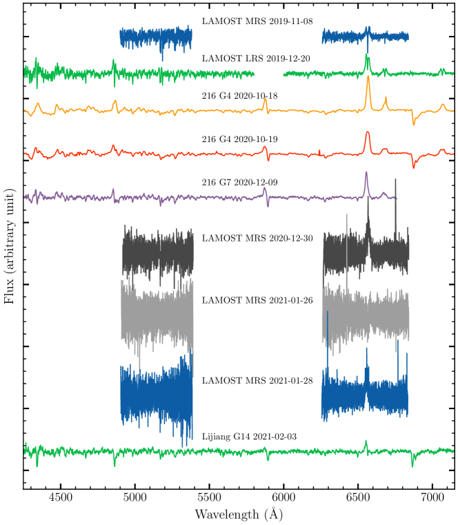
Figure 1: Normalized average spectra of J0419. Each average spectrum is generated by combining the spectra observed on the same night. Prior to the combination, the wavelength has been shifted to rest frame. The observation information is marked next to each average spectrum.

2.1.2 The 2.16-meter telescope spectra

We applied for two spectral observations of J0419 using the 2.16-meter telescope (Fan et al., 2016) at the Xinglong Observatory. The first observations were performed from 2020-10-18 to 2020-10-19, with 16 exposures. We chose the G4 grism and 1.8 slit combination, which yielded an instrumental broadening (FWHM) of 18.4 Å measured from skylines. The resolution is too low to measure the RVs. These spectra show strong Balmer and He I emission lines (see Figure 1).

The second observations were performed on Dec 9, 2020, and the grism was adjusted to G7 to improve the spectral resolution, which yielded an FWHM of 9.0 Å measured from skylines. The spectra also show evident emission lines, albeit the equivalent widths (EW) of the emission lines are less than the first observations.

We used IRAF v2.16 to reduce the spectra with standard process. The heliocentric correction was made using the helcorr function in python package PyAstronomy.

2.1.3 The Lijiang 2.4-meter telescope spectra

On February 3, 2021, we used the Yunnan Faint Object Spectrograph and Camera (YFOSC), which is mounted on the Lijiang 2.4-meter telescope at the Yunnan Observatories of the Chinese Academy of Sciences, to observe J0419. YFOSC is a multifunctional instrument both for photometry and spectroscopy that has a $2k\times 4k$ back-illuminated CCD detector. More information about YFOSC can be found in Lu et al. (2019). A grism G14 and a 1″.0 slit are used, resulting in wavelength coverage of 3800 Å – 7200 Å with a spectral resolution of 6.5 Å measured from skylines. The Lijiang spectrum shows weak Balmer emission lines, and most of the He I emissions cannot even be seen in the spectrum. The data reduction process of the Lijiang data is similar to that of the Xinglong 2.16-meter spectra.

2.2 Photometric data

We collect the light curves of J0419 from several publicly available photometric surveys. The light curves are used to determine the orbital period and analysis the variability (Figure 2). We introduce the photometric data below.

Figure 2: The light curves of J0419. Colors represent different surveys. No outburst events were captured on the light curves.

2.2.1 TESS

TESS observed J0419 in two sectors in 2018 and 2020, respectively, using the FFIs mode. The first sector was taken from 2018-11-15 to 2018-12-11, and the second was from 2020-11-20 to 2020-12-16, with each exposure time of 1426 s, and 475 s, respectively. A total number of 1176 and 3589 points were obtained in the two sectors. We use a python package lightkurve (Lightkurve Collaboration et al., 2018) to reduce the data and get the TESS light curves of J0419. Images with background counts higher than 150 have been eliminated before the light curve extraction, because we cannot obtain reliable flux from these seriously contaminated images. After the visual inspection, we retain 1111 and 3347 points for the first and second observations, respectively. We use a Pixel Level Decorrelation (PLD, see Deming et al. 2015; Luger et al. 2016, 2018) method to remove systematic instrumental trends. The TESS light curves are shown in Figure 3.

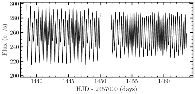
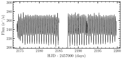
Figure 3: The TESS light curves of J0419. The top panel was observed from 2018-11-15 to 2018-12-11, and the bottom panel was observed from 2020-11-20 to 2020-12-16. The light curve of the top panel shows obvious evolution of the peaks and valleys with time.

2.2.2 ASAS-SN

The ASAS-SN is an automated program to survey the entire visible sky every night down to about 18th magnitude (Shappee et al., 2014; Kochanek et al., 2017). For J0419, ASAS-SN observed the light curve of $V$-band from 2012-02-16 to 2018-11-29 and $G$-band from 2017-09-22 to 2021-07-14. The $V$-band light curve contains 1000 points with a typical uncertainty of 0.051 mag, and the $G$-band light curve contains 1943 points with a typical uncertainty of 0.047 mag. We only include data points with uncertainties less than 0.1 mag, i.e., 895 data points for the $V$-band light curve, and 1656 data points for the $G$-band light curve.

During the ASAS-SN observations, the $V$-band light curve shows a long trend of flux increasing from 2014 to 2020 with an amplitude of about 0.2 mag (see Figure 2). In addition, three points of the ASAS-SN $G$-band light curve near 2019 in Figure 2 far exceed the mean flux range, which raises the suspicion that there is an outburst event. However, the ZTF points observed on the same night have normal fluxes, and there is no sign of outburst of ASAS-SN points observed on adjacent nights. We suspect that the three points are outliers that might be caused by unknown instrumental or data processing problems.

2.2.3 CRTS

J0419 is in the catalog of CRTS with observation time from 2005-10-01 to 2013-10-27. In the eight years of monitoring, CRTS has obtained 394 points. The CRTS monitoring was about 7 years earlier than the ASAS-SN sky survey. During the CRTS monitoring, the light curve was stable and did not show a long-term trend or short-term outburst.

2.2.4 ZTF

We also collected the optical light curve of J0419 from the public DR7 of the ZTF program. The ZTF $g$-band light curve of J0419 has 340 points with a median flux uncertainty of 0.013 mag during the observation from 2018-03-27 to 2021-03-23. The $r$-band has 349 points with median flux uncertainty of 0.012 mag during the observation from 2018-03-28 to 2021-03-28. The ZTF data almost overlaps the $G$-band light curve of ASAS-SN in time coverage but has a higher flux precision.

3 Data analysis

3.1 Gaia information

The Gaia DR3 ID of J0419 is 3298897073626626048. We collect the astrometric information of J0419 from Gaia early data release 3 (EDR3; see Gaia Collaboration et al. 2021), which provide a parallax of $\varpi=1.45\pm 0.03$ mas with proper motions of $\mu_{\alpha}=2.17\pm 0.03$ mas yr^-1 and $\mu_{\delta}=-0.68\pm 0.02$ mas yr^-1. Based on a parallax zero-point correction $zpt=-0.043908$ mas from Lindegren et al. (2021), we obtain a distance of J0419 to the Sun, $d=671.3\pm 12.5\mathrm{~{}pc}$.

Table 2: Orbital and stellar parameters of J0419. The astronomical parameters are from Gaia EDR3. The stellar parameters from SED fitting and spectral fitting are all listed in this table.

Parameter	Unit	Value	Note
The astronomical parameters
R.A.	h:m:s (J2000)	04:19:20.07	Right Ascension
Decl.	d:m:s (J2000)	+07:25:45.4	Declination
Gaia parallax	mas	$1.45\pm 0.03$	The parallax measured by Gaia EDR3
$d(\textit{Gaia~{}})$	pc	$671.3\pm 12.5$	Distance derived from Gaia EDR3
$\mu_{\alpha}$	mas yr-1	$2.17\pm 0.03$	Proper motion in right ascension direction
$\mu_{\delta}$	mas yr-1	$-0.68\pm 0.02$	Proper motion in declination direction
$G$-band magnitude	mag	$14.70\pm 0.01$	The $G$-band magnitude measured by Gaia EDR3
The Orbital parameters
$P_{\mathrm{orb}}$	days	0.6071890(3)	Orbital period
$T_{0}$	HJD	2453644.8439(5)	Ephemeris zero-point
$K_{1}$	$\mathrm{km\,s^{-1}}$	$216\pm 3$	RV semi-amplitude of the visible star
$\gamma$	$\mathrm{km\,s^{-1}}$	$86\pm 3$	The systemic RV of J0419
$f(M_{2})$	$M_{\odot}$	$0.63\pm 0.03$	Mass function of the compact star
Parameters of the pre-ELM
$T_{\mathrm{eff}}$	K	$5793_{-133}^{+124}$	Effective temperature derived from SED fitting
$T_{\mathrm{eff}}$ (spectral fit)	K	$5776\pm 168$	Effective temperature derived from spectral fitting
$\log g$ (spectral fit)	dex	$3.95\pm 0.45$	Surface gravity from spectral fitting
$\log g$	dex	$3.90\pm 0.01$	Surface gravity from SED fitting
Metallicity	$\mathrm{[M/H]}$	$-0.86\pm 0.24$	Metallicity from spectral fitting
$M_{1}$	$M_{\odot}$	$0.176\pm 0.014$	Mass of the visible star
$R_{1}$	$R_{\odot}$	$0.782_{-0.019}^{+0.021}$	Effective radius of the visible star
$L_{\mathrm{bol}}$	$L_{\odot}$	$0.62_{-0.10}^{+0.11}$	Bolometric luminosity of the visible star
$A(V)_{\rm SED}$	mag	$0.34_{-0.10}^{+0.07}$	The extinction value obtained from the SED fitting

3.2 Orbital period

We use the Lomb–Scargle periodogram (Lomb, 1976; Scargle, 1982) to determine the photometric period of J0419. To improve the accuracy of the period value, we use an as-long-as-possible time series from 2005 to 2021 to calculate the Lomb–Scargle power spectrum. We reject the ASAS-SN data for the concerns that the long trend might interfere with the measurement results. The light curves of CRTS, TESS, and ZTF are combined after the flux normalization. We estimate the uncertainty of the period by using a bootstrap method (Efron et al., 1979) that we repeat 10000 times measurements with randomly removing partial points in each measurement. The Lomb–Scargle periodogram gives a period with an error of $P_{\mathrm{orb}}=0.6071890(3)$ days. Note that for the ellipsoidal variation, the real orbital period is twice the peak period on the Lomb–Scargle power spectrum.

In order to determine the zero point of ephemeris $T_{0}$, we use a three-term Fourier model (Morris & Naftilan, 1993),

$$f(t)= a_{0}\cos[\omega(t-T_{0})]+a_{1}\cos[2\omega(t-T_{0})]$$ (1)

$$+a_{2}\cos[3\omega(t-T_{0})],$$

to fit the normalized light curve, where $\omega=2\pi/P_{\mathrm{orb}}$, $a_{0}$, $a_{1}$, $a_{2}$ are the parameters used to fit the light curve profile. We find the best-fitting parameters by minimizing the $\chi^{2}$ statistics, which yield the zero point of ephemeris of $T_{0}=2453644.8439(5)$, where $T_{0}$ corresponds to the superior conjunction. We list $P_{\mathrm{orb}}$ and $T_{0}$ in Table 2. The folded light curves from different surveys or filters using $P_{\mathrm{orb}}$ and $T_{0}$ are shown in Figure 4.

3.3 Photometric variability

The folded light curves (Figure 4) show ellipsoidal variability with amplitudes of about 0.3 mag, together with the evidence of mass transfer (the obvious emission lines in the spectra), indicating that the visible star is already full of the Roche lobe. We did not find any outburst event of this source in the 15 years of photometric monitoring, suggesting that the mass transfer rate is very low. The result is similar to El-Badry et al. (2021a, b) and different to normal CVs.

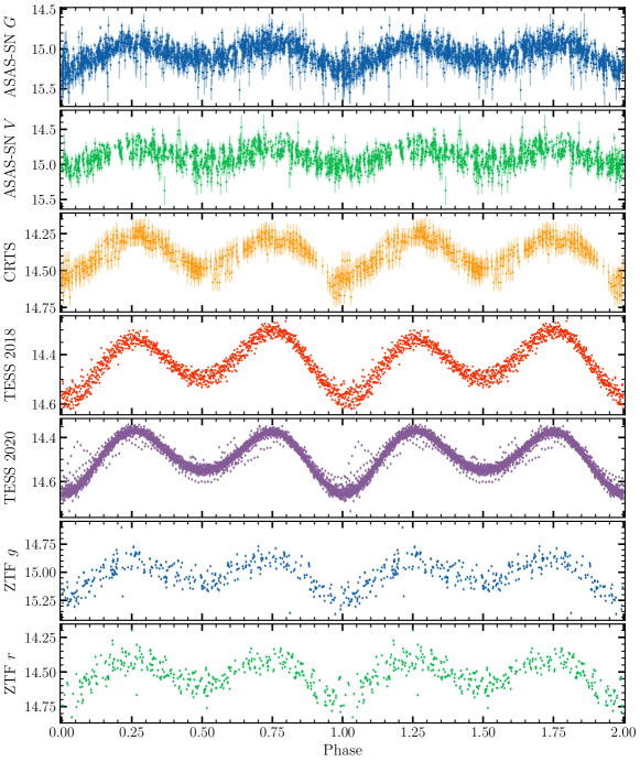
Figure 4: The folded light curves of J0419. The light curves show ellipsoidal variability with a full amplitude of about 0.3 mag. The two sectors of TESS data are shown in two panels, respectively.

The high cadence TESS observation can be used to show the light curve profile at each period. The light curve observed in 2020 (bottom panel of Figure 3) exhibits a typical ellipsoidal variation, while the light curve observed in 2018 (top panel of Figure 3) has a long-term evolution trend of the peaks and valleys beyond the period. The timescale of the evolution seems to be several ten days, which is consistent with the timescale of spot activity (Hussain, 2002; Reinhold et al., 2013). We suspect that the long-term evolution of the light curve observed in 2018 may result from the spot activity.

The folded light curves (except for the TESS data observed in 2020) show larger scatters than the measurement errors (see the ZTF light curves in Figure 4). The extra scatter could be due to multiple reasons. The spot activity we mentioned above may bring about an additional scatter. The flux from the accretion disk may also contribute to the dispersion of the light curves, although the mass transfer rate of J0419 is very low. The temperature and $\log g$ (see Section 3.6) suggest that J0419 falls in the pre-ELM WD instability strip (Córsico et al., 2016; Wang et al., 2020), in which the pulsation can be driven by the $\kappa-\gamma$ mechanism (Unno et al., 1989) and the “convective driving” mechanism (Brickhill, 1991) acting at the H-ionization and He-ionization zones, the scatter may be partly from the pulsation.

3.4 Radial velocities

We obtain the template used to measure RV of each single epoch spectrum of J0419 through a python package PyHammar, and the best-fitting stellar type is G0. The RVs are then measured by using the cross-correlation function (CCF). The uncertainties of the RVs are estimated using the “flux randomization random subset sampling (FR/RSS)” method (Peterson et al., 1998). Only the spectral wavelength from 4910 Å to 5375 Å is used to measure the RVs to avoid the disruption of Balmer and $\rm He~{}I$ emission lines and telluric lines (see Figure 1). Because of the low resolution, the spectra observed by the 2.16-meter telescope using the G4 grism are excluded from the RV measurements.

Figure 5: Radial velocities of the visible star. The period used to fold the RVs is $P_{\mathrm{orb}}=0.607189$ days. The points observed by different telescopes or nights are plotted with different colors and have been labeled at the top left of the panel. A sinusoidal function is used to fit the RVs. The dashed line represents the systemic RV of $\rm\gamma=86$ $\mathrm{km\,s^{-1}}$, and the black solid line is the best-fit RV curve with a semi-amplitude of $K_{1}=216$ $\mathrm{km\,s^{-1}}$

.

We fold the RVs in one phase using the period of $P_{\mathrm{orb}}=0.607189$ days and $T_{0}=2453644.8439$ derived from Section 3.2 and display the result in Figure 5. Since the visible star is full of Roche lobe, the orbital circularization is effective, i.e., the binary moves along a circular orbit (Zahn, 1977). Therefore, we fit the RVs with a circular orbit model following the equation:

$$V(t)=-K_{1}\sin\left[\omega(t+\Delta t)\right]+\gamma,$$ (2)

where $K_{1}$ is the semi-amplitude of RVs of the visible star, $\omega=2\pi/P_{\mathrm{orb}}$, $\gamma$ is the systemic velocity of J0419 to the Sun, and $\Delta t$ represents the possible zero-point shift caused by the limited period accuracy when folding the RVs. The fitting results are $K_{1}=216\pm 3$ $\mathrm{km\,s^{-1}}$, $\gamma=86\pm 3$ $\mathrm{km\,s^{-1}}$, and $\Delta t=12\pm 3$ minutes. We display the RV model curve in Figure 5. The best-fitting RV model well matches the measured RVs.

The mass function of a binary is defined as

$$f(M_{2})=\frac{M_{2}^{3}\sin^{3}i}{(M_{1}+M_{2})^{2}}=\frac{K_{1}^{3}P_{\rm orb}}{2\pi G},$$ (3)

where $M_{1}$ and $M_{2}$ are the mass of the visible star and the compact star, respectively, $K_{1}$ is the semi-amplitude of the RVs of the visible star, $P_{\mathrm{orb}}$ is the orbital period, and $i$ is the inclination angle of the binary to observer. The mass function gives the minimum possible mass of the compact star. Using $P_{\mathrm{orb}}=0.6071890(3)$ days and $K_{1}=216\pm 3$ $\mathrm{km\,s^{-1}}$, we get the mass function of the compact star, $f(M_{2})=0.63\pm 0.03\,M_{\odot}$.

3.5 Spectroscopic stellar parameters

Our spectra were observed in different telescopes or instruments with very different wavelength coverage and resolution. It is difficult to generate a mean spectrum by including all the spectra. Another problem is that most of the spectra have obvious emission lines that may interfere with the measurements of stellar parameters. Therefore, we only use the Lijiang spectrum to take the measurement, which has a good SNR (40.5) and weakest emission lines.

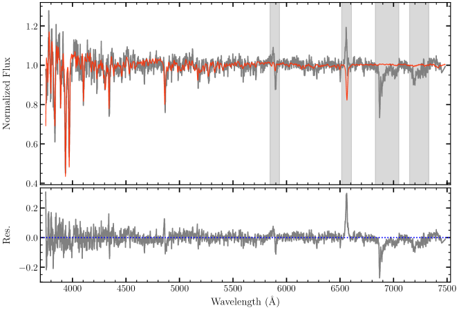
Figure 6: The stellar spectrum fitting result. The gray component in upper panel is the observed spectrum. The red spectrum in upper panel is the model spectrum. The gray component in bottom panel is the residual spectrum. The wavelength of the observed spectrum contaminated by emission lines or telluric lines has been masked before our fitting and shaded with gray in top panel.

We use a python package The_Payne to interpolate the model spectra. The_Payne is a spectral interpolate tool that enable to return a template spectrum when we provide a group of stellar parameters. Based on a neural-net and spectral interpolation algorithm (Ting et al., 2019), The_Payne can interpolate the spectral grid with flexible labels efficiently.

We adopt the BOSZ grid of Kurucz model spectra (Bohlin et al., 2017) with five labels ($T_{\mathrm{eff}}$, $\log g$, $\rm[M/H]$, $\rm[C/M]$, $\rm[\alpha/M]$) to train the template model. The stellar label intervals provided by BOSZ are $\Delta T_{\mathrm{eff}}=250\,\mathrm{K}$, $\Delta\log g=0.5$ dex, $\Delta\mathrm{[Fe/H]=0.25}$ dex. Before the training, we have reduced the resolution of the template to match the resolution of the observed spectrum, and the flux of the template spectra are also normalized using pseudo-continuums that were generated by convolving the template spectra with a gaussian kernel ($\sigma_{\mathrm{width}}=50\,\mathrm{\AA}$).

We construct a likelihood function considering both $\chi^{2}$ and a systematic error,

$$\ln p(f|{\rm\lambda,pms,\sigma_{sys}})=$$ (4)

$$-\frac{1}{2}\sum_{\lambda=\lambda_{0}}^{\lambda_{n}}\left[\frac{(f_{\lambda}-{\rm model}_{\lambda})^{2}}{s_{\lambda}^{2}}+\ln(2\pi s_{\lambda}^{2})\right],$$

where

$$s_{\lambda}^{2}=\sigma_{\lambda}^{2}+\sigma_{\mathrm{sys}}^{2},$$ (5)

$f$ represent the normalized spectrum, $\rm pms$ represent the stellar labels of the template spectrum, $\sigma_{\rm sys}$ is the systematic error. The posteriors of $\rm pms$ and $\sigma_{\rm sys}$ are sampled by the software emcee (Foreman-Mackey et al., 2013) based on the Markov chain Monte Carlo (MCMC) method.

The emcee sampling yield a result of $T_{\rm eff}=5776$ K, $\log g=3.95$ dex, $\rm[M/H]=-0.86$ dex. Similar to Xiang et al. (2019) and El-Badry et al. (2021b), our fitting also underestimate the uncertainties of the stellar parameters with small $\Delta T_{\mathrm{eff}}=56$K, $\Delta\log g=0.19$ dex, $\Delta\mathrm{[M/H]}=0.08$ dex. For simplicity, we directly use $3\sigma$ of the posterior sample as our fitting uncertainties. The fitting results are listed in Table 2.

Figure 6 shows the fitting result of the Lijiang spectrum. The gray spectrum in the top panel is the observation data, and the red spectrum is the best-fitting template. The residual spectrum of $f_{\rm obs}-f_{\rm model}$ is shown in bottom panel. The shadow region in Figure 6 is masked when we perform the fit. We find the model spectrum agrees well with the observed spectrum, except for $\rm H\beta$, $\rm H\alpha$ and several weak $\rm He~{}I$ emission lines clearly showing on the residual spectrum. These emission lines are common in CV spectra (e.g. Sheets et al., 2007). The LAMOST spectra with higher resolution show clear double peak emission lines, which suggest that the emission lines should be produced by the accretion disk rather than the visible star. The emission lines’ equivalent widths (EW) vary greatly in the different observations. If the EWs of the emission lines reflect the mass transfer rate in the binary, the EW variations indicate that the mass transfer process is intermittent. We discuss the emission lines more in Section 4.1.

Our spectra show strong sodium “D” absorption lines beyond the template spectrum at wavelengths of 5890 Å and 5896 Å, which is similar to the result of El-Badry et al. (2021b). Sodium is thought to originate from the CNO-processing that can only reach the surface of a star after most of its envelope has been stripped off. Therefore, sodium enhancement is generally observed in evolved CV donors. The presence of strong sodium absorption lines suggests that the visible star of J0419 is an evolved star and has lost most of its hydrogen envelope.

3.6 The broad-band spectral energy distribution fitting

Survey	Filter	$N_{\mathrm{obs}}$	$\lambda_{\mathrm{effective}}$	AB mag	Vega mag	$\log\lambda f_{\lambda}$
			($\mu m$)	(mag)	(mag)	$\log(\mathrm{erg\ s^{-1}\ cm^{-2}})$
APASS	Johnson $B$	10	0.435		$15.55\pm 0.07$	$-10.787\pm 0.026$
	SDSS $g$	10	0.472	$15.13\pm 0.05$		$-10.689\pm 0.020$
	Johnson $V$	10	0.550		$14.83\pm 0.07$	$-10.633\pm 0.027$
	SDSS $r$	10	0.619	$14.61\pm 0.07$		$-10.597\pm 0.026$
	SDSS $i$	10	0.750	$14.42\pm 0.07$		$-10.606\pm 0.028$
Pan-STARSS	PS1 g	8	0.487	$14.98\pm 0.03$		$-10.643\pm 0.014$
	PS1 $r$	10	0.621	$14.69\pm 0.03$		$-10.633\pm 0.012$
	PS1 $i$	22	0.754	$14.49\pm 0.02$		$-10.637\pm 0.008$
	PS1 $z$	16	0.868	$14.35\pm 0.02$		$-10.641\pm 0.009$
	PS1 $y$	13	0.963	$14.30\pm 0.03$		$-10.669\pm 0.010$
2MASS	2MASS $J$	1	1.241		$13.43\pm 0.1$	$-10.787\pm 0.040$
	2MASS $H$	1	1.651		$13.10\pm 0.1$	$-10.968\pm 0.040$
	2MASS $K_{\mathrm{s}}$	1	2.166		$13.03\pm 0.1$	$-11.243\pm 0.040$
WISE	$\mathrm{W_{1}}$	26	3.379		$12.97\pm 0.02$	$-11.745\pm 0.010$
	$\mathrm{W_{2}}$	26	4.629		$12.91\pm 0.03$	$-12.115\pm 0.011$

Table 3: The SED of J0419. The number of observations is shown in the third column, where the APASS data is a combination of DR9 and DR10. Both APASS and Pan-STARRS data have added additional systematic errors caused by sampling. The magnitudes of 2MASS have been increased by 0.1 mag to correct the phase offset, and the errors have been increased to 0.1 mag. The AB and Vega magnitude systems are displayed in two columns.

We use the broad-band spectral energy distribution (SED) to constrain the stellar parameters and the extinction of J0419. In the SED fitting, the peak wavelength from UV to optical can be used to constrain the effective temperature, $T_{\mathrm{eff}}$. The deviation of the SED slope from Rayleigh-Jeans law in the mid-infrared band is generally considered to be caused by extinction, which can be used to estimate the extinction value (Majewski et al., 2011). The color of $u$-band $v.s.$ other-band represents the metal abundance, $\mathrm{[Fe/H]}$ (Huang et al., 2021). If we know the distance of a source, we can get the effective radius from the SED fitting.

We use a python package astroARIADNE to fit the SED of J0419. astroARIADNE is designed to fit broadband photometry automatically that based on a list of stellar atmosphere models by using the Nested Sampling algorithm. The fitting parameters in astroARIADNE include $T_{\mathrm{eff}}$, $\log g$, [Fe/H], distance, stellar radius, extinction parameter $A(V)$.

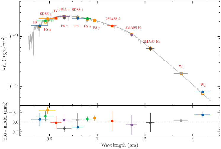
Figure 7: The SED fitting of J0419. The multiband photometric points are plotted in the top panel, and the filter information are displayed near the data points. The model data is also shown in top panel with orange open squares. The model template spectrum is plotted in top panel with gray. The residuals of $f_{\rm obs}-f_{\rm model}$ are plotted in bottom panel.

We collect multi-band photometric data of J0419. Because GALEX (Martin et al., 2005) and $Swift$ (Gehrels et al., 2004) did not observe J0419, we do not have the UV points. The photometric data flag of J0419 in SDSS survey (York et al., 2000) suggest that its magnitudes may have problems. We therefore use the APASS ($B$, $g$, $V$, $r$, and $i$ bands; Henden et al., 2015) data instead. Our photometric data also include Pan-STARRS ($g$, $r$, $i$, $z$, and $y$ bands; Chambers et al., 2016), 2MASS ($J$, $H$, and $K_{\mathrm{s}}$ bands; Skrutskie et al., 2006), and WISE ($\rm W_{1}$, $\rm W_{2}$ bands; Wright et al., 2010).

For the APASS survey, the DR9 data includes six detections, and DR10 includes four detections. We merge these two datasets using the inverse of the error as the weight. For the Pan-STARRS survey, the numbers of single epoch detections in each band are 8, 10, 22, 16, and 13, respectively. Considering that J0419 shows significant variations, we add systematic uncertainties caused by random sampling of the light curves to the errors of the photometric data. The systematic uncertainties in each band are estimated as $\sigma_{\mathrm{sys}}=\mathrm{std}/\sqrt{N}$, where $\mathrm{std}$ is the mean standard deviation of the light curves of J0419, $N$ is the number of observations in a band. 2MASS survey only observed J0419 once on 1999-12-07, 08:27:34.51, and the corresponding phase is 0.28. We assume that the IR band light curve has the same variation amplitude as the optical band to calculate the deviation between the observed magnitude and the mean magnitude and add 0.1 mag to 2MASS data to correct the deviation. Considering the time interval between 2MASS and other surveys (10 to 20 years) and possible light curve trend, we increase the magnitude uncertainties of 2MASS to 0.1 mag. All the photometric data are summarized in Table 3.

The visible star of J0419 has filled the Roche lobe (Section 3.3). In this case, the mean density is given by

$$\bar{\rho}=\frac{3M_{1}}{4\pi R_{1}^{3}}\cong 110P_{\mathrm{hr}}^{-2}\,\mathrm{g\,cm^{-3}},$$ (6)

where $M_{1}$ is the mass, $R_{1}$ is the equivalent radius of the Roche-filling star, the period, $P_{\mathrm{hr}}$, is in the unit of hours (Frank et al., 2002). Equation 6 shows that the mean density of Roche lobe only depends on the orbital period. Combining the radius derived from astroARIADNE fitting and the mean density of Roche lobe, we can calculate the mass and $\log g~{}$of the visible star.

We fit the SED in the following way. First, we use the distance measured by Gaia EDR3 as the prior of distance parameter, and other parameters are set to default values. Then we use the radius from the fitting result to calculate the mass and $\log g$ of the visible star (Equation 6). Second, we update the $\log g~{}$prior by using our calculation and re-fit the SED. $\log g~{}$and $\rm[Fe/H]$ only have little effect on the SED, so the fitting parameters converge quickly. The radius obtained from the SED fitting is $R_{1}=0.782_{-0.019}^{+0.021}\,R_{\odot}$, and the corresponding visible star mass is $M_{1}=0.176\pm 0.014\,M_{\odot}$. The effective temperature of the visible star is $T_{\mathrm{eff}}=5793_{-133}^{+124}\,\mathrm{K}$. The bolometric luminosity derived from the SED fitting is $L_{\mathrm{bol}}=4\pi R_{1}^{2}\,\sigma T_{\mathrm{eff}}^{4}=0.62_{-0.10}^{+0.11}\,L_{\odot}$. We summarize the SED fitting result in Table 2, and show the best fit model in Figure 7.

According to the mass function, $f(M_{2})=0.63\,M_{\odot}$ and the visible star mass $M_{1}=0.176\,M_{\odot}$, we obtain the minimum mass of the compact star, $M_{2}\geq 0.9\,M_{\odot}$. If we assume the compact star is a WD and estimate its radius using the mass-radius relation of Bédard et al. (2020), the corresponding WD radius is $R_{\mathrm{2,max}}<0.01R_{\odot}$. Even if the temperature of the compact star is 20,000 K, its flux contribution in total luminosity is less than 3% and is negligible. The flux contribution from the accretion disk is more complex and will be discussed in Section 4.2. Our analysis in that Section demonstrate that the flux contribution in optical band is dominated by the visible star.

3.7 The light curve fitting

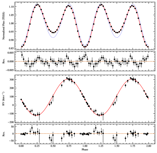
Figure 8: Best-fit light and RV curves. The top panel shows the rebinned TESS light curve (filled circles). The dashed blue curve represents the best-fitting ellipsoidal variability model, which cannot well match the observations. Hence, we add a star spot to the model and refit the TESS light curve, and the best-fitting result is shown as the solid red curve. Indeed, adding a spot improves the fit result greatly. The second panel indicates the residuals between the observed and model fluxes. Our model with a star spot well matches the observed data, and the reduced $\chi^{2}$ is 1.1 (close to 1.0). The third panel displays the RV curve, in which the circles are the observed data, and the solid curve is the best-fitting RV model (with a star spot). The bottom panel presents the residuals between the observed RV curve and the model RV curve.

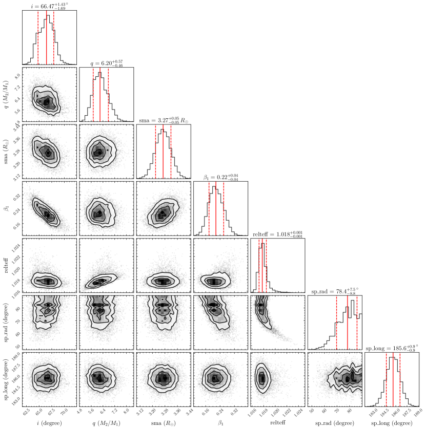
Figure 9: Parameter distributions from the joint fitting of light and RV curves. We only illustrate a fraction of parameters, and other parameters are summarized in Table 4.

J0419 exhibits ellipsoidal variability. The main parameters of modulating the ellipsoidal light curves are the inclination angle $i$, the mass ratio $q=M_{2}/M_{1}$, the filling factor $f_{\mathrm{fill}}$, the limb darkening factors, and the gravity darkening exponent $\beta_{1}$ (von Zeipel, 1924). To estimate the inclination of the binary, we use Phoebe 2.3 (Prša & Zwitter, 2005; Prša et al., 2016; Conroy et al., 2020) to model the light curve and RV curve of J0419, and inversely solve the orbital parameters. Phoebe is an open-source software package, which is based on the Wilson-Devinney software (Wilson & Devinney, 1971), for computing light and RV curves of binaries using a superior surface discretization algorithm. Main physical effects in a binary system have been considered, including eclipse, the distortion of star shape due to the Roche potential, radiative properties (atmosphere intensities, gravity darkening, limb darkening, mutual irradiation), and spots.

In the light curve fitting, we set the temperature of the donor to 5793 K derived from the SED fitting (Section 3.6) with the Phoenix atmosphere model. We adopt the logarithmic limb darkening law and obtain the coefficient values self-consistently from the Phoebe atmosphere model. The gravity darkening law states that, $T_{\mathrm{eff}}^{4}\propto g_{\mathrm{eff}}^{\beta_{1}}$, where $\beta_{1}$ is the gravity darkening exponent. It is generally assumed that, for stars in hydrostatic and radiative equilibrium ($T_{\mathrm{eff}}\gtrsim 8000$ K), $\beta_{1}=1$ (von Zeipel, 1924), and for stars with convective envelopes ($T_{\mathrm{eff}}\lesssim 6300$ K), $\beta_{1}=0.32$ (Lucy, 1967). The theoretical dependence of $\beta_{1}$ upon $T_{\mathrm{eff}}$ is obtained by Claret & Bloemen (2011, see their Figure 2). J0419 appears to be in the temperature range where the transition from convection to equilibrium occurs, therefore we set $\beta_{1}$ as a free parameter and adopt a common normal distribution, $\beta_{1}\sim\mathcal{N}(0.32,0.1)$, as its prior, just similar to El-Badry et al. (2021b).

Because the visible star of J0419 is filling the Roche lobe, we set the model to be semi-detached ($f_{\mathrm{fill}}=1$). We use an equivalent radius of $R_{1}\sim\mathcal{N}(0.78,0.02)\,R_{\odot}$ obtained from the SED fitting as the prior of the radius parameter. The free parameters in our fit are $i$, $q$, $\beta_{1}$, $\gamma$, and sma, where sma is the semi-major axis of a binary orbit.

Except for the second TESS observation data, the folded light curves show larger scatters than the measurement errors. We, therefore, only fit the second TESS data. To reduce the calculation efforts of the model, we rebin the light curve of TESS to 40 points. The errors of the rebinned light curve include both the measurement errors and a systematic error that is estimated using a median filter method (Zhang et al., 2019).

We find that a pure ellipsoidal model cannot well explain the observed data. Indeed, the residuals between the observed and model fluxes depend upon the phases (see Figure 8). Thus, we add a spot to the model to compensate for the phase-dependent residuals. The spot component is defined with four parameters, relteff, radius, colatitude, and longitude. The relteff parameter is the ratio of the spot temperature to the local intrinsic temperature of the star. The radius parameter represents the spot angular radius. The remaining two parameters, colatitude and longitude, indicate the colatitude and longitude of the spot on the stellar surface, respectively. We only set relteff, radius, and longitude to be free parameters. The colatitude is fixed to be 90 degrees. We use the Akaike Information Criterion (AIC) and Bayesian Information Criterion (BIC) to compare the pure ellipsoidal model with the one with a spot. For the model without spot, the AIC and BIC of the best fitting result are -105 and -85, respectively. For the model with a spot, the AIC and BIC of the best fitting result are -282 and -255, respectively. Hence, adding a spot improves the fitting result greatly. Figure 8 illustrates the best fit model with a spot, which is in good agreement with the observed light curve. The residuals between the TESS light curve and the model with a spot are much smaller than the variability amplitude. The light curve residuals in Figure 8 show a weak periodic structure. Considering that the reduced $\chi^{2}$ is 1.1 (close to 1.0), the above structure is statistically insignificant. The fitting yields an inclination angle of $i={66.5}_{-1.7}^{+1.4}$ degrees and a mass of the compact object of $M_{2}={1.09}_{-0.05}^{+0.05}\,M_{\odot}$. Figure 9 illustrates the distributions of the model parameters (see also Table 4). We stress that the inferred inclination angle would not significantly change if we omit the spot component.

Table 4: Parameters from the joint fit of light and RV curves.

Parameter	Value	Parameter	Value
$i$ (deg)	${66.5}_{-1.7}^{+1.4}$	$q$ ($M_{2}/M_{1}$)	${6.2}_{-0.5}^{+0.6}$
sma ($R_{\odot}$)	${3.27}_{-0.05}^{+0.05}$	$\gamma$ ($\mathrm{km\,s^{-1}}$)	${87.5}_{-3.6}^{+3.6}$
$\beta_{1}$	${0.22}_{-0.04}^{+0.04}$	spot relteff	${1.018}_{-0.001}^{+0.001}$
spot radius (deg)	${78}_{-9}^{+8}$	spot long (deg)	${186}_{-1}^{+1}$
t0_rv (minutes)	${11.7}_{-2.8}^{+2.7}$	$R_{1}\,(R_{\odot})$	${0.771}_{-0.022}^{+0.020}$
$M_{1}\,(M_{\odot})$	${0.177}_{-0.015}^{+0.014}$	$M_{2}\,(M_{\odot})$	${1.094}_{-0.049}^{+0.053}$
$K_{1}$ ($\mathrm{km\,s^{-1}}$)	${214.8}_{-3.4}^{+3.4}$

Note. — The spot long is the longitude of the spot, where 0 means that the spot points towards the companion of the binary. The t0_rv parameter accounts for the small phase offset.

4 Discussion

4.1 The properties of the emission lines

J0419 has nine nights of observations, and most of the nights have taken multiple spectra. We normalize each single exposure spectrum and measure the EW of $\rm H\alpha$ emission line after subtracting the continuum component, where we generate the continuum template by using The_Payne with the stellar parameters obtained in Section 3.5. We obtain the EW of the $\rm H\alpha$ emission line by integrating each residual spectrum from 6520 Å to 6610 Å. The EWs of $\rm H\alpha$ are listed in Table 1. As can be seen from Figure 1, the EWs of the $\rm H\alpha$ emission line have changed greatly from night to night. But at the same night, or two nearby observation nights, the EWs change little. These show that the timescale of the variations of emission lines is from several days to tens of days. Some works found the flickering timescale of the emission lines is similar to the continuum in CVs (e.g. Ribeiro & Diaz, 2009), ranging from minutes to hours. The mechanisms of the flicker could be condensations in the matter stream (Stockman & Sargent, 1979), non-uniform mass accretion, or turbulence in the accretion disk (Elsworth & James, 1982). The longer variability timescale of the emission lines of J0419 may be due to the low mass transfer rate.

According to the mass function (Equation 3) and visible star mass, the mass ratio is $q=M_{2}/M_{1}>5.3$. If we assume that the emission lines originate from the accretion disk, the RV semi-amplitude of the emission lines will be $K_{\mathrm{em}}<41.3$ $\mathrm{km\,s^{-1}}$. The resolution and SNR of the J0419 spectra are not enough to measure the RVs of the emission lines. However, we find that the wavelength shift of the emission lines is much smaller than the continuum component, which disfavors the stellar origin of the emission lines.

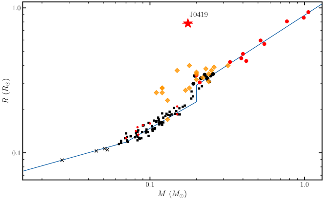
Figure 10: The mass-radius distribution of CVs and pre-ELMs. The red and black points are normal CVs from Patterson et al. (2005). The orange diamond points are pre-ELMs from El-Badry et al. (2021a), and the red star is J0419. The solid line is the mass-radius relation of CVs adopted from Knigge et al. (2011).

4.2 Possible flux from the compact star or disk

The radiation from the companion star or disk for an accreting binary system will lead to an overestimation of the radius and mass of the donor. For J0419, as we mentioned in Section 3.6, due to the large mass of the compact star, its flux contribution in total luminosity is negligible. The radiation from the accretion disk is more complicated. Most normal CVs have strong radiation from disks in the optical band. However, for the evolved donors with higher temperatures, their mass transfer rate is very low (El-Badry et al., 2021a, b) and the donors dominate the luminosities. The spectra of J0419 are also clearly dominated by the donor. We list the reasons below:

1. The SED is well fitted by a pure stellar model;

2. The template spectrum matches well with the observation spectra;

3. The light curves of J0419 show ellipsoidal variability, and no CV characteristics were found, such as violent variability in a short timescale, outburst events.

4.3 Comparison to CVs

Most CVs have low mass donors whose orbital periods are several hours (Section 1). The donors show characteristics similar to main-sequence stars with the same mass as they have the same chemical composition and structure. Unlike normal CVs, the pre-ELMs in CV stage have evolved and do not follow the donor sequence. Evolved donors generally have higher temperatures and possibly more bloated radii than normal CVs with similar donor masses.

We collect the mass and radius data of normal CVs from Patterson et al. (2005), and pre-ELM from El-Badry et al. (2021a), and plot them in Figure 10. The red and black points in Figure 10 are normal CVs; the orange diamond points are pre-ELMs. The solid line is the empirical mass-radius relation of normal CVs from Knigge et al. (2011). J0419 is labeled by the red star for comparison. We can see that J0419 completely deviates from the empirical mass-radius relation of normal CVs. Objects of El-Badry et al. (2021a) either fall on the mass-radius relation or slightly deviate from it, although their temperatures are significantly higher than the normal CV donors with the same mass. These show that the visible star of J0419 is very bloated and more evolved than the objects of El-Badry et al. (2021a).

Compared with normal CVs, the SED of J0419 is dominated by the donor star, and emission lines in the spectra are weaker. No outburst events were detected in 15 years of monitoring. We do not find random variability in a short timescale from hours to days in the high cadence TESS light curves, which is different from the light curves of most normal CVs (Bruch, 2021). The objects of El-Badry et al. (2021a) exhibit similar properties. These indicate that the mass transfer rate of pre-ELM is very low compared with normal CVs.

4.4 Comparison to other pre-ELMs

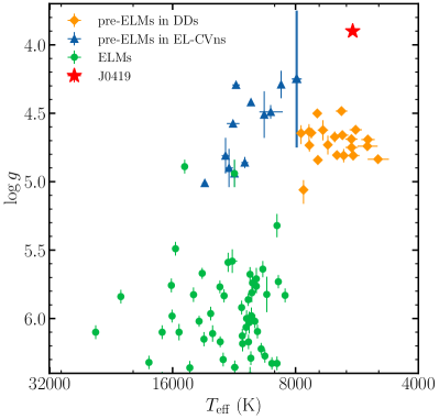
Figure 11: $T_{\mathrm{eff}}-\log g$ diagram of ELMs and pre-ELMs. The meaning of different points is labeled in top left of the panel.

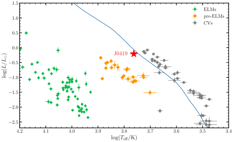
Figure 12: HR diagram. The green points are the ELMs from Brown et al. (2020). The orange diamond points are pre-ELMs from El-Badry et al. (2021a). The gray points are CVs from Knigge (2006). The solid line is the main sequence obtained from isochrones (Morton, 2015). The red star is J0419.

Several works have reported the pre-ELMs. These objects are stripped stars with burning hydrogen envelopes that more bloated and cooler than ELMs. Most of the reported pre-ELMs are found in EL CVns. Their companions are main-sequence A or F stars. We collect ELMs/pre-ELMs to compare their properties. The EL CVn-type stars are from Maxted et al. (2013, 2014a); Córsico et al. (2016); Corti et al. (2016); Gianninas et al. (2016); Zhang et al. (2017); Wang et al. (2020); Lee et al. (2020), the pre-ELMs in DDs are from El-Badry et al. (2021a), and the ELMs are from Brown et al. (2020).

The pre-ELMs in EL-CVns are hotter than pre-ELMs in DDs (see Figure 11), which should be due to the selection effect. Most of the reported EL CVns are detached binaries selected from the eclipse systems. Their radii have been shrinking after the detachment, accompanied by the increase of surface temperatures. The reported pre-ELMs (including J0419 and the sources of El-Badry et al. 2021a) in DDs all have distinct ellipsoidal variability. They are filling or close filling the Roche lobe with lower temperatures. Hence, the pre-ELMs in EL-CVns are at the latter stage of the evolution than the reported pre-ELMs in DDs.

For J0419, its mass and temperature are similar to the sources of El-Badry et al. (2021a). They are all in the transition from mass transfer to detached. Compared with the sources in El-Badry et al. (2021a), J0419 has the smallest surface gravity (see Figure 11), which is due to its far longer orbital period. According to the evolution model of ELMs (Sun & Arras, 2018; Li et al., 2019), pre-ELMs with longer initial periods will be more evolved before the mass transfer begins, resulting in smaller $\log g$ and longer periods. Long-period pre-ELMs like J0419 are rarely reported in previous works.

Similar to El-Badry et al. (2021a, b), we show the position of J0419 on the HR diagram in Figure 12. For comparison, we plot the ELMs obtained from Brown et al. (2020) and the pre-ELM objects obtained from El-Badry et al. (2021a). We also show the CV sample using the data from Ritter & Kolb (2003); Knigge (2006). The solid line in Figure 12 is the main sequence obtained from isochrones (Morton, 2015) with an age of $\rm\log age=8.3$. Most CVs in Figure 12 are fall on the main sequence. Both the ELMs and pre-ELMs are well below the main sequence, showing that they are evolved stripped stars.

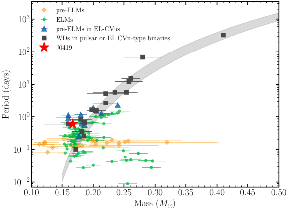
Figure 13: $M_{\mathrm{WD}}-P_{\mathrm{orb}}$ relation. The black squares are helium WDs orbiting pulsars or pre-WDs orbiting an A-type MS star (see Tauris & van den Heuvel, 2014), and the data are obtained from Antoniadis et al. (2012, 2013); van Kerkwijk et al. (2000, 2005, 2010); Maxted et al. (2013); Corongiu et al. (2012); Jacoby et al. (2005); Ransom et al. (2014); Breton et al. (2012); Verbiest et al. (2008); Splaver et al. (2005); Pietrzyński et al. (2012). The blue triangles are pre-ELMs in EL CVns referred to Section 4.4. The green circle points are ELMs reported in Brown et al. (2020). The orange diamonds points are pre-ELMs from El-Badry et al. (2021a). The red star is J0419. The shadow is the $M_{\mathrm{WD}}-P_{\mathrm{orb}}$ relation calculated according to the analytical formula in Tauris & Savonije (1999). The upper and lower limits of the shadow correspond to the metallicities of $\rm Z=0.001-0.02$.

While the pre-ELMs of El-Badry et al. (2021a) deviate significantly from the main sequence, J0419 almost falls on the main sequence, which makes the method of selecting J0419 analogs via HR diagram ineffective. For the J0419 analogs, we can only search for these objects by combining the variation features along with the SED fitting and spectroscopic information, which significantly limits their sample size. The multiple exposure strategy of LAMOST is beneficial to search for such long-period pre-ELMs and binary systems consisting of a visible star and a compact star (Yi et al., 2019).

4.5 The evolutionary properties

According to Sun & Arras (2018); Li et al. (2019), the orbit of J0419 will continue to shrink with angular momentum loss due to the magnetic braking until the convective envelope becomes too thin. After the orbital contraction ends, the accretion process will stop, and the radius of the visible star begins to shrink with increasing temperature and $\log g$. The visible star will gradually evolve into an ELM WD.

The typical temperature of the transition from mass-transferring CVs to detached ELMs is about 6500 K (Sun & Arras, 2018), which is related to the Kraft break (Kraft, 1967). When the temperature is higher than this value, stars will lack the convective envelopes to generate the magnetic field, so that the magnetic braking is no longer effective. The sample of El-Badry et al. (2021a) well verifies this statement. In their sample, the emission lines only occur in the sources with $T_{\mathrm{eff}}<6600$ K, and the sources with higher temperatures have no emission lines found. J0419 with the donor temperature of $T_{\mathrm{eff}}=5793$ K seems also obey the law.

The evolution of ELMs mainly depends on the initial mass of the visible star and the initial orbital period. The stars in WD + MS binaries with sufficiently long initial periods will ascend to the red giant branch when the mass transfer begins. The orbits of such systems will expand with the mass transfer (above the bifurcation period, see Figure 6 of Li et al. 2019). For the donors just leaving the main sequence when mass transfer begins, their orbits will shrink due to the magnetic braking. Both the mass and period of J0419 appear to be in between these two cases.

For WDs in binaries beyond the bifurcation period, there is a tight relationship between the core mass of a low mass giant and the radius of its envelope, resulting in a good correlation between the period and the core mass at the termination of mass transfer (Rappaport et al., 1995). For systems below the bifurcation period ($P_{\mathrm{orb}}\lesssim 16-22$ h, $M_{\mathrm{core}}\lesssim 0.18M_{\odot}$), the correlation between the radius and mass of the donors is unclear.

Figure 13 shows the mass—period distribution of helium stars. The long-period systems are radio pulsar binaries or EL CVn-type systems, and most of the short-period objects are ELM/pre-ELMs reported in recent years. J0419 is just at the junction of the upper and the lower systems. With a mass of $M_{1}=0.176\pm 0.014M_{\odot}$ and a period of $P_{\mathrm{orb}}=0.607189$ days, J0419 appears to follow the $M_{\mathrm{WD}}-P_{\mathrm{orb}}$ relation. The proprieties of closing to the bifurcation period and ongoing mass transfer make J0419 a unique source to connect ELM/pre-ELM systems, wide binaries, and CVs. The systems with periods longer than 14 hours well follow the $M_{\mathrm{WD}}-P_{\mathrm{orb}}$ relation. But for short period targets, the correlation becomes diffuse. The sources with short periods and relatively large mass at the bottom of Figure 13 are thought to be generated through CE channel (Li et al., 2019).

5 Summary

We report a pre-ELM, J0419, consisting of a visible star and a compact star selected from the LAMOST medium-resolution survey with a period of $P_{\mathrm{orb}}=0.607189$ days. The follow-up spectroscopic observations provide a RV semi-amplitude of the visible star, $K_{1}=216\pm 3$ $\mathrm{km\,s^{-1}}$, yielding a mass function of $f(M_{2})=0.63\pm 0.03M_{\odot}$. Both the large-amplitude ellipsoidal variability and the emission lines in the spectra indicate that the visible star has filled the Roche lobe. We use the mean density of the Roche lobe (only depending on the orbital period) and the radius of the visible star obtained from the SED fitting to calculate the mass of the visible star, which yields a mass of $M_{1}=0.176\pm 0.014\,M_{\odot}$. The visible star mass is significantly lower than the expected mass of a star with a G-type spectrum, indicating that the donor of J0419 is an evolved star, i.e., a pre-ELM. By fitting both the light and RV curves using Phoebe, we obtain an inclination angle of $i=66.5_{-1.7}^{+1.4}$ degrees, corresponding to the compact object mass of $M_{2}=1.09\pm 0.05\,M_{\odot}$. We find that J0419 has many features that are similar to the pre-ELM sample in El-Badry et al. (2021a), such as the visible star mass, temperature, the low mass transfer rate. However, the orbital period of J0419 is about three times the mean period of the sample in El-Badry et al. (2021a). We list the main properties of J0419 below:

• J0419 has a more evolved donor than the objects of El-Badry et al. (2021a). The surface gravity of the visible star, $\log g=3.9$, is smaller than known pre-ELM systems, showing that the visible star of J0419 is very bloated (see Section 4.4 and Figure 11).

• J0419 shows clear signatures of mass transfer. With a temperature of $T_{\mathrm{eff}}=5793_{-133}^{+124}$K, J0419 seems to obey the empirical relation in El-Badry et al. (2021a) that the low-temperature pre-ELMs ($T_{\mathrm{eff}}<6500\sim 7000$ K) have mass transfer, but the pre-ELMs with higher temperature have no mass transfer. The phenomenon is generally considered to be caused by the magnetic braking becoming inefficient to take away the angular momentum, and the donors shrink inside their Roche lobe (see Section 4.5).

• According to the evolutionary model of Li et al. (2019), we suspect that J0419 may be a rare source close to the bifurcation period of orbit evolution and therefore did not shrink or expand its orbit significantly (see Section 4.5 and Figure 13).

• J0419 is close to the main sequence, which makes the selection of the long-period pre-ELMs like J0419 based on the HR diagram inefficient. Our work demonstrates a unique way to select such pre-ELMs by combining time-domain photometric and spectroscopic observations (see Figure 12).

6 Acknowledgements

We thank Fan Yang, Honggang Yang, and Weikai Zong for beneficial discussions, and thank the anonymous referee for constructive suggestions that improved the paper. This work was supported by the National Key R&D Program of China under grant 2021YFA1600401, and the National Natural Science Foundation of China under grants 11925301, 12103041, 12033006, 11973002, 11988101, 11933004, 12090044, 11833006, U1831205, and U1938105. This paper uses the LAMOST spectra. We also acknowledge the support of the staff of the Xinglong 2.16-meter telescope and Lijiang 2.4-meter telescope.

References

- Amaro-Seoane et al. (2012) Amaro-Seoane, P., Aoudia, S., Babak, S., et al. 2012, Classical and Quantum Gravity, 29, 124016, doi: 10.1088/0264-9381/29/12/124016
- Antoniadis et al. (2012) Antoniadis, J., van Kerkwijk, M. H., Koester, D., et al. 2012, MNRAS, 423, 3316, doi: 10.1111/j.1365-2966.2012.21124.x
- Antoniadis et al. (2013) Antoniadis, J., Freire, P. C. C., Wex, N., et al. 2013, Science, 340, 448, doi: 10.1126/science.1233232
- Bédard et al. (2020) Bédard, A., Bergeron, P., Brassard, P., & Fontaine, G. 2020, ApJ, 901, 93, doi: 10.3847/1538-4357/abafbe
- Beuermann et al. (1998) Beuermann, K., Baraffe, I., Kolb, U., & Weichhold, M. 1998, A&A, 339, 518. https://arxiv.org/abs/astro-ph/9809233
- Bohlin et al. (2017) Bohlin, R. C., Mészáros, S., Fleming, S. W., et al. 2017, AJ, 153, 234, doi: 10.3847/1538-3881/aa6ba9
- Breton et al. (2012) Breton, R. P., Rappaport, S. A., van Kerkwijk, M. H., & Carter, J. A. 2012, ApJ, 748, 115, doi: 10.1088/0004-637X/748/2/115
- Brickhill (1991) Brickhill, A. J. 1991, MNRAS, 251, 673, doi: 10.1093/mnras/251.4.673
- Brown et al. (2016) Brown, W. R., Gianninas, A., Kilic, M., Kenyon, S. J., & Allende Prieto, C. 2016, ApJ, 818, 155, doi: 10.3847/0004-637X/818/2/155
- Brown et al. (2013) Brown, W. R., Kilic, M., Allende Prieto, C., Gianninas, A., & Kenyon, S. J. 2013, ApJ, 769, 66, doi: 10.1088/0004-637X/769/1/66
- Brown et al. (2010) Brown, W. R., Kilic, M., Allende Prieto, C., & Kenyon, S. J. 2010, ApJ, 723, 1072, doi: 10.1088/0004-637X/723/2/1072
- Brown et al. (2012) —. 2012, ApJ, 744, 142, doi: 10.1088/0004-637X/744/2/142
- Brown et al. (2011) Brown, W. R., Kilic, M., Hermes, J. J., et al. 2011, ApJ, 737, L23, doi: 10.1088/2041-8205/737/1/L23
- Brown et al. (2020) Brown, W. R., Kilic, M., Kosakowski, A., et al. 2020, ApJ, 889, 49, doi: 10.3847/1538-4357/ab63cd
- Bruch (2021) Bruch, A. 2021, MNRAS, 503, 953, doi: 10.1093/mnras/stab516
- Carter et al. (2011) Carter, J. A., Rappaport, S., & Fabrycky, D. 2011, ApJ, 728, 139, doi: 10.1088/0004-637X/728/2/139
- Chambers et al. (2016) Chambers, K. C., Magnier, E. A., Metcalfe, N., et al. 2016, arXiv e-prints, arXiv:1612.05560. https://arxiv.org/abs/1612.05560
- Chen et al. (2017) Chen, X., Maxted, P. F. L., Li, J., & Han, Z. 2017, MNRAS, 467, 1874, doi: 10.1093/mnras/stx115
- Claret & Bloemen (2011) Claret, A., & Bloemen, S. 2011, A&A, 529, A75, doi: 10.1051/0004-6361/201116451
- Conroy et al. (2020) Conroy, K. E., Kochoska, A., Hey, D., et al. 2020, ApJS, 250, 34, doi: 10.3847/1538-4365/abb4e2
- Corongiu et al. (2012) Corongiu, A., Burgay, M., Possenti, A., et al. 2012, ApJ, 760, 100, doi: 10.1088/0004-637X/760/2/100
- Córsico et al. (2016) Córsico, A. H., Althaus, L. G., Serenelli, A. M., et al. 2016, A&A, 588, A74, doi: 10.1051/0004-6361/201528032
- Corti et al. (2016) Corti, M. A., Kanaan, A., Córsico, A. H., et al. 2016, A&A, 587, L5, doi: 10.1051/0004-6361/201527458
- Cui et al. (2012) Cui, X.-Q., Zhao, Y.-H., Chu, Y.-Q., et al. 2012, Research in Astronomy and Astrophysics, 12, 1197, doi: 10.1088/1674-4527/12/9/003
- Czesla et al. (2019) Czesla, S., Schröter, S., Schneider, C. P., et al. 2019, PyA: Python astronomy-related packages, Astrophysics Source Code Library, record ascl:1906.010. http://ascl.net/1906.010
- Deming et al. (2015) Deming, D., Knutson, H., Kammer, J., et al. 2015, ApJ, 805, 132, doi: 10.1088/0004-637X/805/2/132
- Drake et al. (2009) Drake, A. J., Djorgovski, S. G., Mahabal, A., et al. 2009, ApJ, 696, 870, doi: 10.1088/0004-637X/696/1/870
- Drake et al. (2014) Drake, A. J., Graham, M. J., Djorgovski, S. G., et al. 2014, ApJS, 213, 9, doi: 10.1088/0067-0049/213/1/9
- Efron et al. (1979) Efron, R., Yund, E. W., & Divenyi, P. L. 1979, Acoustical Society of America Journal, 66, 75, doi: 10.1121/1.382974
- El-Badry et al. (2021a) El-Badry, K., Rix, H.-W., Quataert, E., Kupfer, T., & Shen, K. J. 2021a, MNRAS, doi: 10.1093/mnras/stab2583
- El-Badry et al. (2021b) El-Badry, K., Quataert, E., Rix, H.-W., et al. 2021b, MNRAS, 505, 2051, doi: 10.1093/mnras/stab1318
- Elsworth & James (1982) Elsworth, Y. P., & James, J. F. 1982, MNRAS, 198, 889, doi: 10.1093/mnras/198.4.889
- Fan et al. (2016) Fan, Z., Wang, H., Jiang, X., et al. 2016, PASP, 128, 115005, doi: 10.1088/1538-3873/128/969/115005
- Foreman-Mackey et al. (2013) Foreman-Mackey, D., Hogg, D. W., Lang, D., & Goodman, J. 2013, PASP, 125, 306, doi: 10.1086/670067
- Frank et al. (2002) Frank, J., King, A., & Raine, D. J. 2002, Accretion Power in Astrophysics: Third Edition
- Gaia Collaboration et al. (2021) Gaia Collaboration, Brown, A. G. A., Vallenari, A., et al. 2021, A&A, 649, A1, doi: 10.1051/0004-6361/202039657
- Gehrels et al. (2004) Gehrels, N., Chincarini, G., Giommi, P., et al. 2004, ApJ, 611, 1005, doi: 10.1086/422091
- Gianninas et al. (2016) Gianninas, A., Curd, B., Fontaine, G., Brown, W. R., & Kilic, M. 2016, ApJ, 822, L27, doi: 10.3847/2041-8205/822/2/L27
- Gianninas et al. (2014) Gianninas, A., Dufour, P., Kilic, M., et al. 2014, ApJ, 794, 35, doi: 10.1088/0004-637X/794/1/35
- Gianninas et al. (2015) Gianninas, A., Kilic, M., Brown, W. R., Canton, P., & Kenyon, S. J. 2015, ApJ, 812, 167, doi: 10.1088/0004-637X/812/2/167
- Han & Podsiadlowski (2004) Han, Z., & Podsiadlowski, P. 2004, MNRAS, 350, 1301, doi: 10.1111/j.1365-2966.2004.07713.x
- Henden et al. (2015) Henden, A. A., Levine, S., Terrell, D., & Welch, D. L. 2015, in American Astronomical Society Meeting Abstracts, Vol. 225, American Astronomical Society Meeting Abstracts #225, 336.16
- Huang et al. (2021) Huang, Y., Yuan, H., Li, C., et al. 2021, ApJ, 907, 68, doi: 10.3847/1538-4357/abca37
- Hussain (2002) Hussain, G. A. J. 2002, Astronomische Nachrichten, 323, 349
- Istrate et al. (2014a) Istrate, A. G., Tauris, T. M., & Langer, N. 2014a, A&A, 571, A45, doi: 10.1051/0004-6361/201424680
- Istrate et al. (2014b) Istrate, A. G., Tauris, T. M., Langer, N., & Antoniadis, J. 2014b, A&A, 571, L3, doi: 10.1051/0004-6361/201424681
- Jacoby et al. (2005) Jacoby, B. A., Hotan, A., Bailes, M., Ord, S., & Kulkarni, S. R. 2005, ApJ, 629, L113, doi: 10.1086/449311
- Kalomeni et al. (2016) Kalomeni, B., Nelson, L., Rappaport, S., et al. 2016, ApJ, 833, 83, doi: 10.3847/1538-4357/833/1/83
- Kepler et al. (2015) Kepler, S. O., Pelisoli, I., Koester, D., et al. 2015, MNRAS, 446, 4078, doi: 10.1093/mnras/stu2388
- Kesseli et al. (2017) Kesseli, A. Y., West, A. A., Veyette, M., et al. 2017, ApJS, 230, 16, doi: 10.3847/1538-4365/aa656d
- Kilic et al. (2011) Kilic, M., Brown, W. R., Allende Prieto, C., et al. 2011, ApJ, 727, 3, doi: 10.1088/0004-637X/727/1/3
- Kilic et al. (2012) —. 2012, ApJ, 751, 141, doi: 10.1088/0004-637X/751/2/141
- Kilic et al. (2015) Kilic, M., Hermes, J. J., Gianninas, A., & Brown, W. R. 2015, MNRAS, 446, L26, doi: 10.1093/mnrasl/slu152
- Knigge (2006) Knigge, C. 2006, MNRAS, 373, 484, doi: 10.1111/j.1365-2966.2006.11096.x
- Knigge et al. (2011) Knigge, C., Baraffe, I., & Patterson, J. 2011, ApJS, 194, 28, doi: 10.1088/0067-0049/194/2/28
- Kochanek et al. (2017) Kochanek, C. S., Shappee, B. J., Stanek, K. Z., et al. 2017, PASP, 129, 104502, doi: 10.1088/1538-3873/aa80d9
- Kosakowski et al. (2020) Kosakowski, A., Kilic, M., Brown, W. R., & Gianninas, A. 2020, ApJ, 894, 53, doi: 10.3847/1538-4357/ab8300
- Kraft (1967) Kraft, R. P. 1967, ApJ, 150, 551, doi: 10.1086/149359
- Lee et al. (2020) Lee, J. W., Koo, J.-R., Hong, K., & Park, J.-H. 2020, AJ, 160, 49, doi: 10.3847/1538-3881/ab9621
- Li et al. (2019) Li, Z., Chen, X., Chen, H.-L., & Han, Z. 2019, ApJ, 871, 148, doi: 10.3847/1538-4357/aaf9a1
- Lightkurve Collaboration et al. (2018) Lightkurve Collaboration, Cardoso, J. V. d. M., Hedges, C., et al. 2018, Lightkurve: Kepler and TESS time series analysis in Python, Astrophysics Source Code Library. http://ascl.net/1812.013
- Lindegren et al. (2021) Lindegren, L., Bastian, U., Biermann, M., et al. 2021, A&A, 649, A4, doi: 10.1051/0004-6361/202039653
- Liu et al. (2020) Liu, C., Fu, J., Shi, J., et al. 2020, arXiv e-prints, arXiv:2005.07210. https://arxiv.org/abs/2005.07210
- Lomb (1976) Lomb, N. R. 1976, Ap&SS, 39, 447, doi: 10.1007/BF00648343
- Lu et al. (2019) Lu, K.-X., Bai, J.-M., Zhang, Z.-X., et al. 2019, ApJ, 887, 135, doi: 10.3847/1538-4357/ab5790
- Lucy (1967) Lucy, L. B. 1967, ZAp, 65, 89
- Luger et al. (2016) Luger, R., Agol, E., Kruse, E., et al. 2016, AJ, 152, 100, doi: 10.3847/0004-6256/152/4/100
- Luger et al. (2018) Luger, R., Kruse, E., Foreman-Mackey, D., Agol, E., & Saunders, N. 2018, AJ, 156, 99, doi: 10.3847/1538-3881/aad230
- Luo et al. (2016a) Luo, A. L., Zhao, Y. H., Zhao, G., et al. 2016a, VizieR Online Data Catalog, V/149
- Luo et al. (2016b) Luo, J., Chen, L.-S., Duan, H.-Z., et al. 2016b, Classical and Quantum Gravity, 33, 035010, doi: 10.1088/0264-9381/33/3/035010
- Majewski et al. (2011) Majewski, S. R., Zasowski, G., & Nidever, D. L. 2011, ApJ, 739, 25, doi: 10.1088/0004-637X/739/1/25
- Martin et al. (2005) Martin, D. C., Fanson, J., Schiminovich, D., et al. 2005, ApJ, 619, L1, doi: 10.1086/426387
- Masci et al. (2019) Masci, F. J., Laher, R. R., Rusholme, B., et al. 2019, PASP, 131, 018003, doi: 10.1088/1538-3873/aae8ac
- Maxted et al. (2014a) Maxted, P. F. L., Serenelli, A. M., Marsh, T. R., et al. 2014a, MNRAS, 444, 208, doi: 10.1093/mnras/stu1465
- Maxted et al. (2011) Maxted, P. F. L., Anderson, D. R., Burleigh, M. R., et al. 2011, MNRAS, 418, 1156, doi: 10.1111/j.1365-2966.2011.19567.x
- Maxted et al. (2013) Maxted, P. F. L., Serenelli, A. M., Miglio, A., et al. 2013, Nature, 498, 463, doi: 10.1038/nature12192
- Maxted et al. (2014b) Maxted, P. F. L., Bloemen, S., Heber, U., et al. 2014b, MNRAS, 437, 1681, doi: 10.1093/mnras/stt2007
- Morris & Naftilan (1993) Morris, S. L., & Naftilan, S. A. 1993, ApJ, 419, 344, doi: 10.1086/173488
- Morton (2015) Morton, T. D. 2015, isochrones: Stellar model grid package, Astrophysics Source Code Library, record ascl:1503.010. http://ascl.net/1503.010
- Mu et al. (2022) Mu, H.-J., Gu, W.-M., Yi, T., et al. 2022, Science China Physics, Mechanics, and Astronomy, 65, 229711, doi: 10.1007/s11433-021-1809-8
- Patterson (1984) Patterson, J. 1984, ApJS, 54, 443, doi: 10.1086/190940
- Patterson et al. (2005) Patterson, J., Kemp, J., Harvey, D. A., et al. 2005, PASP, 117, 1204, doi: 10.1086/447771
- Peterson et al. (1998) Peterson, B. M., Wanders, I., Bertram, R., et al. 1998, ApJ, 501, 82, doi: 10.1086/305813
- Pietrzyński et al. (2012) Pietrzyński, G., Thompson, I. B., Gieren, W., et al. 2012, Nature, 484, 75, doi: 10.1038/nature10966
- Podsiadlowski et al. (2003) Podsiadlowski, P., Han, Z., & Rappaport, S. 2003, MNRAS, 340, 1214, doi: 10.1046/j.1365-8711.2003.06380.x
- Prša & Zwitter (2005) Prša, A., & Zwitter, T. 2005, ApJ, 628, 426, doi: 10.1086/430591
- Prša et al. (2016) Prša, A., Conroy, K. E., Horvat, M., et al. 2016, ApJS, 227, 29, doi: 10.3847/1538-4365/227/2/29
- Ransom et al. (2014) Ransom, S. M., Stairs, I. H., Archibald, A. M., et al. 2014, Nature, 505, 520, doi: 10.1038/nature12917
- Rappaport et al. (2015) Rappaport, S., Nelson, L., Levine, A., et al. 2015, ApJ, 803, 82, doi: 10.1088/0004-637X/803/2/82
- Rappaport et al. (1995) Rappaport, S., Podsiadlowski, P., Joss, P. C., Di Stefano, R., & Han, Z. 1995, MNRAS, 273, 731, doi: 10.1093/mnras/273.3.731
- Reinhold et al. (2013) Reinhold, T., Reiners, A., & Basri, G. 2013, A&A, 560, A4, doi: 10.1051/0004-6361/201321970
- Ribeiro & Diaz (2009) Ribeiro, F. M. A., & Diaz, M. P. 2009, PASJ, 61, 137, doi: 10.1093/pasj/61.1.137
- Ricker et al. (2015) Ricker, G. R., Winn, J. N., Vanderspek, R., et al. 2015, Journal of Astronomical Telescopes, Instruments, and Systems, 1, 014003, doi: 10.1117/1.JATIS.1.1.014003
- Ritter & Kolb (2003) Ritter, H., & Kolb, U. 2003, A&A, 404, 301, doi: 10.1051/0004-6361:20030330
- Roulston et al. (2020) Roulston, B. R., Green, P. J., & Kesseli, A. Y. 2020, ApJS, 249, 34, doi: 10.3847/1538-4365/aba1e7
- Scargle (1982) Scargle, J. D. 1982, ApJ, 263, 835, doi: 10.1086/160554
- Shappee et al. (2014) Shappee, B. J., Prieto, J. L., Grupe, D., et al. 2014, ApJ, 788, 48, doi: 10.1088/0004-637X/788/1/48
- Sheets et al. (2007) Sheets, H. A., Thorstensen, J. R., Peters, C. J., Kapusta, A. B., & Taylor, C. J. 2007, PASP, 119, 494, doi: 10.1086/518698
- Skrutskie et al. (2006) Skrutskie, M. F., Cutri, R. M., Stiening, R., et al. 2006, AJ, 131, 1163, doi: 10.1086/498708
- Smith & Dhillon (1998) Smith, D. A., & Dhillon, V. S. 1998, MNRAS, 301, 767, doi: 10.1046/j.1365-8711.1998.02065.x
- Splaver et al. (2005) Splaver, E. M., Nice, D. J., Stairs, I. H., Lommen, A. N., & Backer, D. C. 2005, ApJ, 620, 405, doi: 10.1086/426804
- Stockman & Sargent (1979) Stockman, H. S., & Sargent, T. A. 1979, ApJ, 227, 197, doi: 10.1086/156719
- Sun & Arras (2018) Sun, M., & Arras, P. 2018, ApJ, 858, 14, doi: 10.3847/1538-4357/aab9a4
- Tauris & Savonije (1999) Tauris, T. M., & Savonije, G. J. 1999, A&A, 350, 928. https://arxiv.org/abs/astro-ph/9909147
- Tauris & van den Heuvel (2014) Tauris, T. M., & van den Heuvel, E. P. J. 2014, ApJ, 781, L13, doi: 10.1088/2041-8205/781/1/L13
- Ting et al. (2019) Ting, Y.-S., Conroy, C., Rix, H.-W., & Cargile, P. 2019, ApJ, 879, 69, doi: 10.3847/1538-4357/ab2331
- Tody (1986) Tody, D. 1986, in Society of Photo-Optical Instrumentation Engineers (SPIE) Conference Series, Vol. 627, Instrumentation in astronomy VI, ed. D. L. Crawford, 733, doi: 10.1117/12.968154
- Tody (1993) Tody, D. 1993, in Astronomical Society of the Pacific Conference Series, Vol. 52, Astronomical Data Analysis Software and Systems II, ed. R. J. Hanisch, R. J. V. Brissenden, & J. Barnes, 173
- Unno et al. (1989) Unno, W., Osaki, Y., Ando, H., Saio, H., & Shibahashi, H. 1989, Nonradial oscillations of stars
- van der Sluys et al. (2005) van der Sluys, M. V., Verbunt, F., & Pols, O. R. 2005, A&A, 431, 647, doi: 10.1051/0004-6361:20041777
- van Kerkwijk et al. (2005) van Kerkwijk, M. H., Bassa, C. G., Jacoby, B. A., & Jonker, P. G. 2005, in Astronomical Society of the Pacific Conference Series, Vol. 328, Binary Radio Pulsars, ed. F. A. Rasio & I. H. Stairs, 357. https://arxiv.org/abs/astro-ph/0405283
- van Kerkwijk et al. (2000) van Kerkwijk, M. H., Bell, J. F., Kaspi, V. M., & Kulkarni, S. R. 2000, ApJ, 530, L37, doi: 10.1086/312478
- van Kerkwijk et al. (2010) van Kerkwijk, M. H., Rappaport, S. A., Breton, R. P., et al. 2010, ApJ, 715, 51, doi: 10.1088/0004-637X/715/1/51
- Verbiest et al. (2008) Verbiest, J. P. W., Bailes, M., van Straten, W., et al. 2008, ApJ, 679, 675, doi: 10.1086/529576
- Vines & Jenkins (2022) Vines, J. I., & Jenkins, J. S. 2022, MNRAS, doi: 10.1093/mnras/stac956
- von Zeipel (1924) von Zeipel, H. 1924, MNRAS, 84, 665, doi: 10.1093/mnras/84.9.665
- Wang et al. (2018) Wang, K., Luo, C., Zhang, X., et al. 2018, AJ, 156, 187, doi: 10.3847/1538-3881/aade52
- Wang et al. (2020) Wang, K., Zhang, X., & Dai, M. 2020, ApJ, 888, 49, doi: 10.3847/1538-4357/ab584c
- Wilson & Devinney (1971) Wilson, R. E., & Devinney, E. J. 1971, ApJ, 166, 605, doi: 10.1086/150986
- Wright et al. (2010) Wright, E. L., Eisenhardt, P. R. M., Mainzer, A. K., et al. 2010, AJ, 140, 1868, doi: 10.1088/0004-6256/140/6/1868
- Xiang et al. (2019) Xiang, M., Ting, Y.-S., Rix, H.-W., et al. 2019, ApJS, 245, 34, doi: 10.3847/1538-4365/ab5364
- Yi et al. (2019) Yi, T., Sun, M., & Gu, W.-M. 2019, ApJ, 886, 97, doi: 10.3847/1538-4357/ab4a75
- York et al. (2000) York, D. G., Adelman, J., Anderson, John E., J., et al. 2000, AJ, 120, 1579, doi: 10.1086/301513
- Zahn (1977) Zahn, J. P. 1977, A&A, 57, 383
- Zhang et al. (2017) Zhang, X. B., Fu, J. N., Liu, N., Luo, C. Q., & Ren, A. B. 2017, ApJ, 850, 125, doi: 10.3847/1538-4357/aa9577
- Zhang et al. (2019) Zhang, Z.-X., Du, P., Smith, P. S., et al. 2019, ApJ, 876, 49, doi: 10.3847/1538-4357/ab1099
- Zhao et al. (2012) Zhao, G., Zhao, Y.-H., Chu, Y.-Q., Jing, Y.-P., & Deng, L.-C. 2012, Research in Astronomy and Astrophysics, 12, 723, doi: 10.1088/1674-4527/12/7/002
- Zong et al. (2018) Zong, W., Fu, J.-N., De Cat, P., et al. 2018, ApJS, 238, 30, doi: 10.3847/1538-4365/aadf81