Numerical Study of S=1/2 Heisenberg Antiferromagnet
on the Floret Pentagonal Lattice

Abstract

The $S=1/2$ Heisenberg antiferromagnet on the floret-pentagonal lattice with two kinds of interaction strength is studied by the numerical-diagonalization method. It is known that, near the five-ninth of the saturation magnetization, this system shows a magnetization jump that is not accompanied by magnetization plateaux. We focus our attention on the behavior of this system around the five-ninth of the saturation magnetization; the changes of the magnetization jump and plateau at and around this magnetization are clarified from the diagonalization data for finite-size systems up to 45 sites.

1 Introduction

Frustration in magnetic materials has attracted much attention of many condensed-matter physicists. The frustration is typically caused by a local structure of antiferromagnetic interactions forming a polygon with an odd number of sides – an odd-gon – . The simplest case is the triangular structure; magnetism on various lattices including such triangular structure, for example, the triangular lattice and the kagome lattice, have been extensively and intensively studied. The next possibility for the odd-gon is a pentagon. However, a relatively much smaller number of investigations have been carried out for the magnetism of a system on a pentagonal lattice. As such a two-dimensional pentagonal lattice, the Cairo-pentagonal-lattice Heisenberg antiferromagnet was studied and the system shows the characteristic magnetization process with magnetization plateaux and jumps[1, 2, 3]. Note here that candidate materials for the Cairo-pentagonal-lattice antiferromagnet were studied recently[4, 5, 6, 7, 8]. As systems including local pentagonal structure, studies concerning spherical kagome cluster[9], dodecahedral cluster[10, 11], and icosidodecahedron cluster [12, 13] are also known.

Recently, the floret-pentagonal-lattice (FPL) antiferromagnet was investigated[14] as the second two-dimensional case among pentagonal lattices. The FPL Heisenberg antferromagnet shows magnetization plateaux in its magnetization process at one-ninth, one-third, and seven-ninth of the saturation magnetization. The magnetization plateaux are related to the number of spin sites in each unit cell of this lattice, namely, nine. Spin sites of the FPL are divided into two groups; a coordination number of sites on one group is six and that on the other group is three. Let us consider antiferromagnetic interaction bonding a site of coordination number to be six ($J_{1}$) and antiferromagnetic interaction not bonding such sites ($J_{2}$). Reference References reported that the magnetization plateaux at one-third and seven-ninth of the saturation magnetization get smaller and close when $J_{2}/J_{1}$ is increased.

Let us we focus our attention on the behavior of the FPL antiferromagnet at and near the five-ninth of the saturation magnetization. In the uniform case, the FPL antiferromagnet does not show a magnetization plateau at this magnetization; on the other hand, the system shows a peculiar magnetization jump near this magnetization. Under these circumstances, the purpose of this study is to clarify the behavior near this magnetization during the variation of $J_{2}/J_{1}$ by the Lanczos-diagonalization method for finite-size clusters of this system. We successfully capture the appearance the magnetization jump near this magnetization in a specific range of $J_{2}/J_{1}$. We also find that the magnetization plateau at five-ninth of the saturation appears for $J_{2}/J_{1}$ that is larger than a specific value of this ratio.

This paper is organized as follows. In the next section, the model Hamiltonian will be introduced. The method of calculations will also be explained. The third section is devoted to the presentation and discussion of our results concerning the magnetization jump near the five-ninth of the saturation. In the fourth section, we discuss the appearance of the magnetization plateau at this magnetization. In the final section, a summary of our results and some remarks will be given.

2 Model and calculation

We investigate the $S=1/2$ Heisenberg antiferromagnet on the FPL. The Hamiltonian of the investigated model is described by ${\cal H}={\cal H}_{0}+{\cal H}_{\mathrm{zeeman}}$ where

$${\cal H}_{0} = \sum_{\rm{solid\hskip 2.0ptbonds}}J_{1}\mbox{\boldmath$S$}_{i}\cdot\mbox{\boldmath$S$}_{j}+\sum_{\rm{dotted\hskip 2.0ptbonds}}J_{2}\mbox{\boldmath$S$}_{i}\cdot\mbox{\boldmath$S$}_{j},\ {\cal H}_{\rm zeeman}=-h\sum_{j}S_{j}^{z}.$$ (1)

Here, $\mbox{\boldmath$S$}_{i}$ denotes the $S=1/2$ spin operator at site $i$ illustrated by the closed circle at a vertex in Fig. 1(a). In the first term of Eq. (1), the sum is taken for the bonds depicted by the solid line in Fig. 1(a), and in the second term, the sum is taken for the bonds depicted by the dotted line. Energies are measured in units of $J_{1}$ in Eq. (1). Since we examine the case of antiferromagnetic interaction, we put $J_{1}=1$, $J_{2}>0$ hereafter. We define $\eta=J_{2}/J_{1}$ as the ratio of these interactions. In the case $\eta=1$, all interactions are equivalent, when the behavior of this system was studied in Ref. References. In that case, some nontrivial phenomena due to frustration were reported. In the present study, we investigate what happens when $\eta$ is varied concerning the phenomena that were observed in Ref. References.

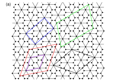
Figure 1: Panel (a) shows the floret-pentagonal lattice and finite-size clusters treated in this study. Solid and broken lines denote interaction with amplitude $J_{1}$ and $J_{2}$, respectively. Violet, blue, black, red, and green solid lines correspond to the finite-size clusters for $N=9$, $18$, $27$, $36$, and $45$, respectively. Panel (b) shows groups of vertices: $\alpha$, $\beta$, and $\gamma$.

Figure 1(a) also shows the shape of finite size clusters treated in the present study. The number of spin sites is denoted as $N$. Note that the finite-size clusters for $N=9$, $27$, and $36$ are rhombic, whereas those for $N=18$ and $45$ are not rhombic. Although these nonrhombic clusters therefore show symmetries that are different from the FPL, calculations of $N=18$ and $45$ contribute to deepen our understanding of the FPL antiferromagnet. In all the finite-size clusters, the periodic boundary condition is employed. Note also that the magnetization process for a 45-site cluster was first reported in the case of the kagome-lattice antiferromagnet[15] and that the present study for the FPL antiferromagnet is the second report of a 45-site magnetization process to the best of our knowledge.

The FPL has originally been known in the tiling problem[16]. Figure 1(b) shows the grouping of vertices of this lattice. A unit cell of the FPL contains nine vertices, which are divided into two groups at first. One is a group of vertices of the type characterized by the coordination number $z=6$ and the other group consists of vertices with $z=3$. The former vertex is called $\alpha$ sites, and the latter is further divided into two groups: those linked by a bond with $\alpha$ are called $\beta$ sites, and those not linked are called $\gamma$ sites.

In this study, the ground-state energy of ${\cal H}_{0}$ is calculated in the subspace characterized by $M$ defined by $\sum_{j}S_{j}^{z}$. The calculation to obtain the energy by diagonalizing ${\cal H}_{0}$ is based on the Lanczos algorithm and/or the Householder algorithm. The energy is denoted by $E(N,M)$. The saturation value of $M$ is defined as $M_{\rm s}(=SN)$, until which $M$ increases discretely with $\delta M=1$. The magnetization process is determined so that the magnetization increases from $M$ to $M+1$ at magnetic field $h=E(N,M+1)-E(N,M)$ when the magnetization monotonically increases with $h$. When the monotonic increase disappears, there appears a jump; the Maxwell construction should be carried out to capture the behavior of the jump. We evaluate local magnetization $m_{\rm loc}$ defined as $(1/N_{\xi})\sum_{j\in\xi}\langle S_{j}^{z}\rangle$, where $\xi$ takes $\alpha$, $\beta$, and $\gamma$; $\langle{\cal O}\rangle$ represents the expectation value of an operator ${\cal O}$ with respect to the lowest-energy state within the subspace with a fixed $M$ of interest. For simplicity, here, we define $m=M/M_{\rm{s}}$ as the normalized magnetization. Part of Lanczos diagonalizations has been performed using the MPI-parallelized code, which was originally developed in the research of the Haldane gaps[17]. The usefulness of our program was demonstrated in several large-scale parallelized calculations[18, 19, 20, 21].

3 Magnetization jump

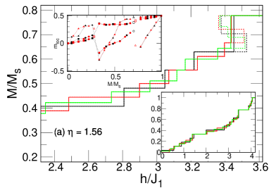
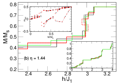
Figure 2: Panels (a) and (b) show the magnetization process and local magnetization for $\eta=1.56$ and $1.44$, respectively. The green, red, and black lines and dots represent results for $N=45$, $36$, and $27$ systems, respectively. The main panel shows a magnified view around the magnetization jump; the solid lines depict the magnetization process after the Maxwell construction is applied. The dashed lines depict the results before the Maxwell construction is applied, which explicitly show unrealized states. The lower-right inset depicts the magnetization process in the entire range up to the saturation. The upper-left inset shows the averaged local magnetization in each system for the rhombic clusters for $N=36$ and 27. The averaging is carried out among each of groups, $\alpha$, $\beta$, and $\gamma$ sites that are represented by triangles, squares, and circles, respectively. Open symbols indicate skipped states because these states do not become a ground state even under any magnetic fields although closed symbols indicate realized states.

Recall here that in the system with $\eta=1$, a jump for the $N=36$ cluster appears as a skipped case of $m=11/18$[14]. This jump is significantly different from jumps that have been reported in many other frustrate systems. Such magnetization jumps are associated with a specific magnetization plateau. However, the jump of the $N=36$ FPL-antiferromagnetic cluster at $m=11/18$ appears away from both the plateaux at $m=1/3$ and 7/9. In this section, we clarify what happens in the magnetization process of this model by observing the change of this jump when $\eta$ is varied.

Now, let us consider the cases for larger $\eta$; results of magnetization processes for $N=27$, $36$, and $45$ are depicted in Fig. 2 for $\eta=1.56$ and 1.44 in panel (a) and (b), respectively. Figure 2 presents the magnetization processes in the entire range in the lower-right inset and a zoom-in view near the jump in the main panel. Let us examine the change of the magnetization process when $\eta$ is decreased. Recall before observing Fig. 2 that the $m=7/9$ plateau begins to open around $\eta\sim 1.6$[14]. For $\eta=1.56$, there appears a magnetization jump at the lower-edge of the $m=7/9$ plateau in Fig. 2(a). For $\eta=1.44$, next, the magnetization jump departs from the $m=7/9$ plateau.

Next, let us observe the relationship between the change of the magnetization jump and averaged local magnetizations $m_{\rm loc}$ in the upper-left insets of Fig. 2. In particular, a marked behavior appears in the results of $m_{\rm loc}$ for $\alpha$ sites. For $\eta=1.56$, the clear discontinuous behavior of $m_{\rm loc}$ in $\alpha$-site results is observed between data at $m=7/9$ and those for $0.6<m<0.7$. For $\eta=1.44$, on the other hand, states for $m\sim 0.6$ actually are realized as the ground states under a specific magnetic field. The results of $m_{\rm loc}$ of $\alpha$ sites in these states and $m_{\rm loc}$ at $m=7/9$ show a continuous behavior. At the same time, there still exists a discontinuous behavior across the jump around $m\sim 0.6$. On the other hand, there are no significant changes in the spin states around $m\sim 0.5$.

From observing the behavior of this system in Fig. 2, the jump originally begins to appear in an association with the opening of the plateau at $m=7/9$ when $\eta$ is decreased from a large-$\eta$ side. In even smaller $\eta$, there appear new states between the jump and the $m=7/9$ plateau under the situation that the jump still survives. Therefore, the new states play an essential role in the formation of the magnetization jump away from any magnetization plateaux.

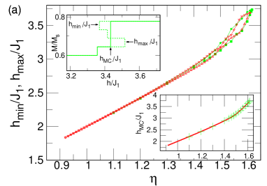
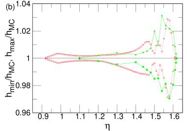
Figure 3: The $\eta$-dependence of the magnetic fields before and after the Maxwell construction ($h_{\rm{min}}$, $h_{\rm{max}}$, and $h_{\rm{MC}}$) for the appearing target jump, where the upper-left inset of panel (a) illustrates $h_{\rm{min}}$, $h_{\rm{max}}$, and $h_{\rm{MC}}$. Main panel (a) shows the $\eta$-dependence of $h_{\rm{min}}/J_{1}$ by open triangles and closed squares and $h_{\rm{max}}/J_{1}$ by open inverted triangles and closed diamonds; the lower-right inset shows that of $h_{\rm{MC}}/J_{1}$ by closed circles and crosses. Green and red symbols represent results for $N=45$ and $36$ systems, respectively. Panel (b) shows the $\eta$-dependence of $h_{\rm{min}}/h_{\rm{MC}}$ and $h_{\rm{max}}/h_{\rm{MC}}$.

To clarify the range of $\eta$ where the magnetization jump discussed in the previous paragraph, let us present the $\eta$-dependence of magnetic fields at the jump before and after the Maxwell construction, where the fields are denoted by $h_{\rm{min}}$, $h_{\rm{max}}$, and $h_{\rm{MC}}$ illustrated in the upper-left inset of Fig. 3(a); results are depicted in Fig. 3(a). When we focus our attention on the edges of this range, there appears the jump in the region of $\eta$ up to $\eta=1.618$ for the $N=45$ and $\eta=1.611$ for the $N=36$. The size difference of this value of $\eta$ is quite small. On the other hand, the jump appears in the region down to $\eta\sim 1.1$ for the $N=45$ and $\eta=0.92$ for the $N=36$; the size dependence is relatively larger than the other edge.

Next, let us observe the behavior inside the range in Fig. 3. One can find a change around $\eta\sim 1.5$ concerning the moving of these fields characterizing the jump $h_{\rm{min}}/J_{1}$, $h_{\rm{max}}/J_{1}$, and $h_{\rm{MC}}/J_{1}$. Note markedly that there is no significant difference in $\eta\sim 1.5$ of the change among $h_{\rm{min}}/J_{1}$, $h_{\rm{max}}/J_{1}$, and $h_{\rm{MC}}/J_{1}$. In particular, $h_{\rm{MC}}/J_{1}$ clearly shows the difference between the regions $\eta<1.5$ and $\eta>1.5$, namely, the gradient in $\eta<1.5$ differs from that in $\eta>1.5$. To clarify the differenece, let us observe $h_{\rm{max}}/h_{\rm{MC}}$ and $h_{\rm{min}}/h_{\rm{MC}}$ show in Fig. 3(b). These behaviors observed in Fig. 3 suggest that the properties of the magnetization jump are different between $\eta>1.5$ and $\eta<1.5$. It is reasonable that the change of $h_{\rm{min}}$ around $\eta\sim 1.5$ comes from the appearance of the new states between the jump and the $m=7/9$ plateau; however, there also appears the change of $h_{\rm{max}}$ almost at the same $\eta$, which suggests that the properties of the magnetization jump change. It is still unclear at the present why the change of the jump appears only in the present model; the reason should be studied in future studies.

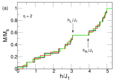
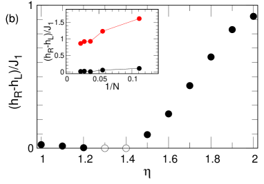
Figure 4: Panel (a) depicts the magnetization process for $\eta=2$ where the green, red, and black lines represent results for $N=45$, $36$, and $27$ systems respectively. In the main panel (b), $\eta$-dependence of the width of $m=5/9$ in the magnetization process of $N=36$ cluster is depicted. Closed and open circles correspond to the cases when the $m=5/9$ states to be realized and unrealized under a specific magnetic field, respectively. Namely, the cases of the open circles indicate the appearance of the magnetization jump. Inset of panel (b) depicts size-dependence of the $m=5/9$ widths. The red (black) lines and symbols represent the results for $\eta=1$ ($\eta=2$).

4 Appearance of the $m=5/9$ plateau

Let us review the appearance of plateaux in the case of all the interactions are equivalent, namely $\eta=1$. Reference References reported that for $\eta=1$, no indication is detected for the plateau at $m=5/9$ although there appear plateaux at $m=7/9$, 1/3, and 1/9.

Now, let us consider the behavior at $m=5/9$ when $\eta$ is varied. First, we present the magnetization process for $\eta=2$; results for $N=45$, 36, and 27 are depicted in Fig. 4(a). One easily finds an existing plateau at $m=5/9$. We define $h_{\rm L}$ ($h_{\rm R}$) as the lower-field (higher-field) edge of $m=5/9$. In the following, let us examine the width of $m=5/9$ namely, $h_{\rm L}-h_{\rm R}$.

In the inset of Fig. 4(b), next, the $N$-dependence of this width for $\eta=2$ together with the case of $\eta=1$. Although the width for $\eta=2$ gradually decreases as $N$ is increased, an extrapolated value of the width to the thermodynamic limit seems nonzero, which suggests the $m=5/9$ plateau certainly opens. For $\eta=1$, in contrast, finite-size widths are much smaller than those for $\eta=2$; an extrapolated value of these finite-size results seems to vanish. These different situations from $\eta=2$ and 1 suggest that the $m=5/9$ plateau closes in a value of intermediate $\eta$ when $\eta$ is decreased from $\eta=2$.

In order to observe the behavior, let us observe results of the width for $N=36$ between $\eta=1$ and 2 in the main panel of Fig. 4(b). With decreasing $\eta$, the width gradually deceases down to $\eta\sim 1.5$. At $\eta\sim 1.4$, finally, the case of $m=5/9$ encounters the magnetization jump moving from higher $m$ and becomes skipped in the magnetization process. Below $\eta\sim 1.2$, the case of $m=5/9$ recovers its width; however, the width still shows a small value due to a finite-size effect. It is noticeable that the magnetization plateau at $m=5/9$ appears for large $\eta$ whereas it disappears for small $\eta$ and that the situation of $m=5/9$ is clearly different from those of $m=7/9$ and 1/3 reported in Ref. References.

5 Summary

We have studied the $S=1/2$ Heisenberg antiferromagnet on the floret-pentagonal lattice by using the numerical diagonalization method. The model is controlled by the ratio of two interactions, each of which is determined by the different coordination numbers of spin sites. Our numerical-diagonalization calculations up to the 45-site cluster have clarified the behavior around the five-ninth of the saturation magnetization. Further investigations concerning the system on various pentagonal lattices will contribute much to our understanding frustration effects in magnetic materials.

References

- [1] I. Rousochatzakis, A. M. Luchli, and R. Moessner, Phys. Rev. B 85, 104415 (2012).
- [2] H. Nakano, M. Isoda, and T. Sakai, J. Phys. Soc. Jpn. 83, 053702 (2014).
- [3] M. Isoda, H. Nakano, and T. Sakai, J. Phys. Soc. Jpn. 83, 084710 (2014).
- [4] A. M. Abakumov, D. Batuk, A. A. Tsirlin, C. Prescher, L. Dubrovinsky, D. V. Sheptyakov, W. Schnelle, J. Hadermann, and G. Van Tendeloo, Phys. Rev. B 87, 024423 (2013).
- [5] A. A. Tsirlin, I. Rousochatzakis, D. Filimonov, D. Batuk, M. Frontzek, and A. M. Abakumov, Phys. Rev. B 96, 094420 (2017).
- [6] S. Chattopadhyay, S. Petit, E. Ressouche, S. Raymond, V. Baldent, G. Yahia, W. Peng, J. Robert, M.-B. Lepetit, M. Greenblatt, and P. Foury-Leylekian, Sci. Rep. 7, 14506 (2017).
- [7] J. Cumby, R. D. Bayliss, F. J. Berry, and C. Greaves, Dalton Trans. 45, 11801 (2016).
- [8] K. Beauvois, V. Simonet, S. Petit, J. Robert, F. Bourdarot, M. Gospodinov, A. A. Mukhin, R. Ballou, V. Skumryev, E. Ressouche, Phys. Rev. Lett. 124, 127202 (2020).
- [9] N. Kunisada and Y. Fukumoto, Prog. Theor. Exp. Phys. 2014, 041I01 (2014).
- [10] N. P. Konstantinidis, Phys. Rev. B 72, 064453 (2005).
- [11] N. P. Konstantinidis, J. Phys.: Condens. Matter 28, 016001 (2016).
- [12] M. Exler and J. Schnack, Phys. Rev. B 67, 094440 (2003).
- [13] C. Schroder, H. Nojiri, J. Schnack, P. Hage, M. Luban, and P. Kogerler, Phys. Rev. Lett. 94, 017205 (2005).
- [14] R. Furuchi, H. Nakano, N. Todoroki, and T. Sakai, J. Phys. Commun. 5, 125008 (2021).
- [15] H. Nakano and T. Sakai, J. Phys. Soc. Jpn. 87, 063706 (2018).
- [16] D. Schattschneider, Mathematics Magazine 51, 29 (1978).
- [17] H. Nakano and A. Terai, J. Phys. Soc. Jpn. 78, 014003 (2009).
- [18] H. Nakano and T. Sakai, J. Phys. Soc. Jpn. 80, 053704 (2011). [Errata 90, 038002 (2021)]
- [19] H. Nakano and T. Sakai, J. Phys. Soc. Jpn. 87, 123702 (2018).
- [20] H. Nakano, N. Todoroki, and T. Sakai, J. Phys. Soc. Jpn. 88, 114702 (2019).
- [21] H. Nakano, H. Tadano, N. Todoroki, and T. Sakai, J. Phys. Soc. Jpn. 91, 074701 (2022).