Variance Tolerance Factors For Interpreting All Neural Networks
Abstract
Black box models only provide results for deep learning tasks, and lack informative details about how these results were obtained. Knowing how input variables are related to outputs, in addition to why they are related, can be critical to translating predictions into laboratory experiments, or defending a model prediction under scrutiny. In this paper, we propose a general theory that defines a variance tolerance factor (VTF) inspired by influence function, to interpret features in the context of black box neural networks by ranking the importance of features, and construct a novel architecture consisting of a base model and feature model to explore the feature importance in a Rashomon set that contains all well-performing neural networks. Two feature importance ranking methods in the Rashomon set and a feature selection method based on the VTF are created and explored. A thorough evaluation on synthetic and benchmark datasets is provided, and the method is applied to two real world examples predicting the formation of noncrystalline gold nanoparticles and the chemical toxicity 1793 aromatic compounds exposed to a protozoan ciliate for 40 hours.
Index Terms:
black box model, feature importance, Rashomon sets, influence functionI Introduction
Machine learning is a powerful tool that can learn and describe the patterns behind data, enabling researchers to make predictions and improve decisions [1]. This advanced technology has been widely employed in scientific disciplines, e.g. psychology, physics and genomics, but many problems are solved using box machine learning models and big datasets that are not representative [2]. Knowing the prediction results or a single metric, such as classification accuracy, is insufficient for describing tasks [3] and inappropriate for studies in the sciences where predictions must be accountable. For example, the effectiveness of a medical treatment for a patient may be predictable, but how and why the prediction was made is also an important part of the patient record. Interpretability and unambiguous explanations of the model can be crucial.
The definition of interpretability is hard to be established. Miller [4] and Kim [5] described the interpretability “the degree to which a human can comprehend the cause of a decision”. Humans can understand the behavior and predictions of machine learning by using transparent methods or interpretable methods. Feature importance rankings that measure the contribution of the input variables to the prediction hava become an important tool in interpretable machine learning [6]. These ranking methods are often associated with feature selection, as features can be selected or eliminated based on the rankings to provide an optimal subset [7]. Intuitively, if a model can “tell” which features are important to itself, the machine learning system would benefit from a subset of optimal features by reducing the dimensionality (improving efficiency), improving the generalizability of the learning system [8, 9, 10] and simplifying accountability. It was argued that focusing solely on explaining a pre-specific black box model is unjustifiable according to recent research [2, 11], and it would be more appropriate to explore the feature importance in all well-performing models. These are the primary motivations of this study.
In this paper, we defined the variance tolerance factor (VTF) that evaluates model’s tolerance to features’ variance in a Rashomon set that contains accurate neural networks, and proposed a novel model-agnostic framework based on it to address the lack of interpretability in neural networks [12, 13], where the contribution of the input variables (features) in predicting the output (target) is opaque. Two model-agnostic methods are devised; one from data-driven perspective and one based on mathematical principles. Our architecture consists of a “base model” and a “feature model”, where the base model can be constructed in any format based on the type of task (classification or regression). The two models are trained sequentially and the feature model is systematically re-trained until it achieves the same performance as the base task. After training, the base model is fixed and the weights of a mask layer in the feature model provides the general feature importance recognised by the model. These weights can be further processed as the basis for fast feature selection and interpretable ranking methods using domain knowledge. Each method is thoroughly evaluated on synthetic, benchmark and real datasets via representative machine learning models (e.g. Linear Regression, Logistic Regression, Multilayer Perceptron, Convolutional Neural Network and Recurrent Neural Network) and the study demonstrates the flexibility and interpretability of our framework 111The Supporting Information with code can be found in https://github.com/Sichao-Li/Variance-Tolerance-Factors-for-Interpreting-All-Good-Neural-Networks.
II Related Work
Interpretable machine learning methods are normally categorized as model-specific interpretation methods and model-agnostic interpretation methods [14]. It’s easy to achieve interpretability by using algorithms that create interpretable models, e.g. linear regression, logistic regression and decision trees. The great advantage of model-agnostic interpretation methods that separate the explanations from the machine learning mode is their flexibility [15]. Model-agnostic interpretation methods can be further categorized as global interpretation methods and local interpretation methods. Global methods describe the average behavior of a machine learning model, such as permutation feature importance [16], the partial dependence plot [17], functional decomposition and global surrogate. In contrast, local interpretation methods explain individual predictions. Shapley values from game theory are an example of a method used to explain individual predictions [18]. These methods report models’ interpretations through feature importance ranking. The importance of features are defined differently based on various algorithms: filter-based methods, e.g. SPEC [19] and Fisher Score [20], feature discriminative capability, e.g. ReliefF [21] and statistics-based methods , e.g. T-Score [22]. The wrapper-based methods depend on the accuracy of specific models and evaluate all the possible combinations of features against the evaluation criterion, which usually suffer the problem of high computation complexity [23]. Embedded methods are model-specific and use their own built-in feature selection methods, similar to model-specific methods discussed above. Learning attention used to indicate the feature importance is proved successful in the past [24]. To obtain a more complete understanding of feature importance for a set of different models with equally accurate predictive power, defined as Rashomon set [25], researchers started exploring the set where all models with loss below a threshold [26, 11]. In this paper, our aim is to propose a new view of exploring the Rashomon set for neural networks and interpret the feature importance using information from the set.
III Theorems and methods
III-1 Rashomon set
Given a model class F, the black box model with the minimum loss and the pre-defined tolerance , the Rashomon set is defined as:
| (1) |
III-2 Variance Tolerance Factor (VTF)
VTF measures the sensitivity of a model to changes in the features space by exploring the model class of the Rashomon set . The idea behind the searching method is to explore the feature space by modifying the distributions, instead of model space like conventional methods, as the structure and parameters of black box remain unknown in this context. Details are discussed in section III-B.
By scaling all features simultaneously and quantifying the impact without influencing the model performance, we can find a Rashomon set without prior knowledge of the model information. Then we defined VTF, inspired by the influence function, as the influence of scaling training feature on the parameters.
| (2) |
Where is the notation of VTF and is the scaling factor. The logic behind why influence function can be used in features is roughly reasoned here: researchers [27, 28] have proved the success in application of influence function on a group of instances. When the group contains all instances in the dataset and perturbing all instances in the same way, the process can be seen as perturbing features, evidence provided in the Supporting Information.
Then we can conclude that if the model performance is unaffected by large scaling factors, the model can’t tolerate much variance in such features and then these features are consequentially important. As the parameters are always changing from , the VTF can be further simplified as . If the VTF tends to 0, the feature importance tends to 1; i.e. the model is less tolerant to change in this dimension.
III-3 Feature Selection
Based on the VTF, unimportant features can be selected such that the deviation between the factor of a feature and 1 is greater than 1, , and eliminated in linear time, . Specific tasks might apply different thresholds rather than 1.
| (3) |
III-4 Auxiliary mask
To find the VTF, an auxiliary mask is introduced, which enables the feature set to achieve the similar performance on the same model , where and is a dictionary of features. Each can be seen as a neural network in . Then the following performance equivalence equation can be obtained:
| (4) |
where denotes the element-wise product.
III-A Problem Formulation
The problem then becomes ranking the importance of features in through an auxiliary mask . Suppose is a feature set of features and is the corresponding target set. The performance equivalence equation Eqn.4 can be solved as an optimization problem.
| (5) |
is an L2-norm that helps to speed up the optimization process and controls the strength of penalty.
III-B Model Description
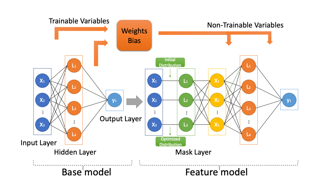
To obtain the mask stated in Eqn.5, we propose a framework consisting of a base model and a feature model, as shown in Fig.1. The base model is selected and employed to accomplish a supervised learning task, e.g., classification or regression, while the feature model is designated to discover the feature importance through a systematic retraining process. The feature model follows the trained base model and fixes the model parameters, while adding an extra mask layer to learn. The feature model is retrained to achieve the loss retrieved from base model and the weights of mask layer are extracted as the output.
Due to the randomness of weights during initialisation, learning rate and other factors, the value of is contingent to a certain extent. Weights can also be misleading with regards to performance. In the case where an unimportant feature is assigned to a high weight, the overall performance is not affected because its contribution to the outcome is virtually insignificant. The weight list in is the final parameter used for the feature selection and feature importance ranking.
III-B1 The choice of initial mask
It is observed that these final mask values depend on the initials used for starting the training process in Supporting Information Proof of learning algorithm. The choice of the initial weights follows 3 principles.
-
•
The weight of each feature must be approximately 0, making sure no initial feature contributions.
-
•
Each feature equally contributes to the model.
-
•
The weight is randomly chosen so that each iteration commences differently.
In summation, the initial weights are distributed as , so that the contribution of each feature is not identical but minor differences can be ignored and the final weight accumulates the effect of all connection weights across all hidden neurons in the network.
Two model-agnostic methods are devised based on VTF for interpreting the model with domain knowledge in the Rashomon set.
III-C Recursive Variance Tolerance Weight (RVTW)
From a VTF point of view, the scaling factors (weights) of the important features tends to 1 as the model restricts the change of the feature instances in training at global level. On the other hand, important features statistically generate greater weights, for example in linear regression, where increasing the value of a feature by one unit changes the estimated outcome by its weight.
To be more convincing we use a data processing strategy that averages a list of weights from repeatedly retraining of the feature model until the average of the weights reaches a stable point. The weight is also scaled with its standard error to mitigate the uncertainty, because if the model performance is unaffected by large variations in the scaling factors, then the feature is consequentially unimportant.
| (6) |
where the value of is the measurement of feature importance, is the number of training times, is the coefficient of the feature at training time . is the standard error .
III-D Contribution Factor (CF)
Considering the equivalence of Eqn.4, another way to approach it is to solve this as an equation system. For any feature set (number of features is greater or equal to 1) contributing to a model, the contribution can be accumulated, such that:
| (7) |
where is a contribution function.
The idea of CF is to treat each feature contribution as an unknown in an equation and construct a solvable equation system. After the feature retraining, we can immediately derive Eqn.8 based on Eqn.7. A factor is introduced to represent the relationship between the weight and the contribution , and can be derived through experiments. The general case is formulated in Eqn.9. A detailed proof of algorithm is shown in Supporting Information Derive of Contribution Factor.
| (8) |
To construct the equation system the number of retrain attempts must be equal or greater than the number of features, which might result in an overdetermined system. Theoretically, it is enough to solve unknowns in an equation system, given the exact same number of equations, but we need more equations to reduce the effect of bias introduced from unimportant features (discussed above), so that with unknowns and equations: . Matrix reduction is necessary to solve this overdetermined system and Gaussian elimination can be applied. With reduced row echelon form, the equation system can be solved, and the contribution of each feature to the performance can be derived.
| (9) |
IV Proof of Concept
To demonstrate the basic feasibility and reliability of the theory, a linear regressor and logistic classifier are selected as a baseline test. The framework is applied to benchmarks and a real-world dataset to evaluate it against practical problems. All datasets used herein are publicly available and were split into 80% training set and 20% testing set prior to optimization with the same random seed. All models and experiments are conducted using TensorFlow software and their details are tabulated to provide the greatest opportunity for experimental control and reproductivity. Training results are tabulated, or included in learning curves which also quantify any under-fitting or over-fitting. Feature importances are ranked using histograms to give intuitive insights of their effects. To test the reliability and accuracy of the proposed methods, we compare their performance with other well-established methods.
IV-1 Model-agnostic methods
-
•
Fisher Score: selects features based on similarities.
-
•
ReliefF: selects features based on the identification of near-hit and near-miss instances.
-
•
Permutation method: gives another feature importance profile by measuring the increase in the base model prediction error after permuting a feature.
-
•
AFS: attention-based supervised feature selection.
-
•
KernelShap: computes the Shapley values that fairly distributes the prediction to each individual feature.
IV-2 Model-specific methods
-
•
Random Forest (RF): regressor provides feature importance based on Gini impurity.
-
•
Connection weights: calculates the sum of products over all hidden layers and ranks the relative importance by the outputs.
IV-3 Evaluation Protocols
To evaluate the performance of feature selection method, the traditional recursive feature elimination (RFE) method is applied to the same model and dataset, with the same feature importance rankings.
Unimportant features are selected according to their importance by percentage, from 10% to 90% and a new model independent from previous training and outputs is used to fit the selected subset. The loss or accuracy of the feature subset indicates the importance of dropped features as the performance metric. For MNIST dataset, we followed the evaluation protocols of [24] to provide a fair comparison.
IV-A Linear Regression and Logistic Regression
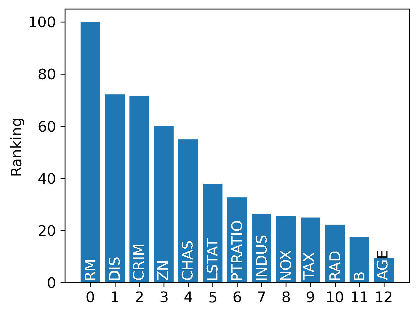
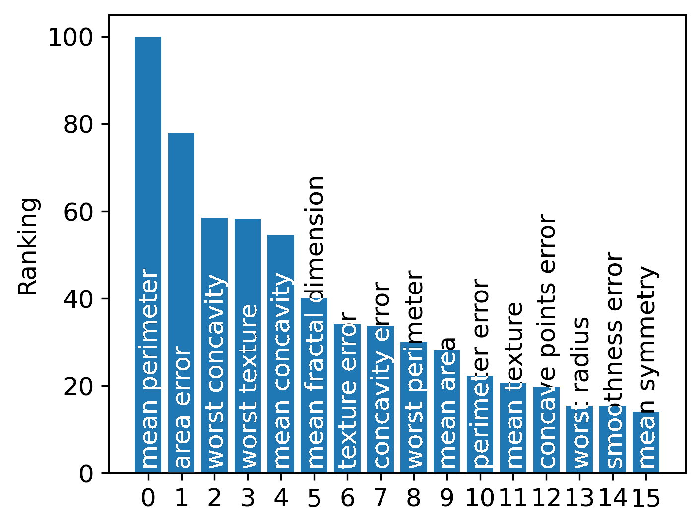
The dataset used in the linear regression is The Boston Housing Dataset [29], which was collected in 1978 and contains information about houses from various suburbs in Boston, Massachusetts. The dataset can be accessed from the scikit-learn library [30], including 506 samples and 13 feature variables. The dataset used in the logistic regression is Breast Cancer Wisconsin (Diagnostic) Dataset [31], which was collected in 1955 and contains information about characteristics of the cell nuclei present in the image of a fine needle aspirate (FNA) of a breast mass. The dataset can be accessed from the scikit-learn library [30], including 569 samples and 30 features.
A linear regressor and a logistic classifier are built to model the relationship between independent variables and one dependent variable. The model and training details are in Supporting Information Table.2. The base model was first trained with all features to make the decision for 1000 epochs, achieving low testing errors and high accuracies, with no over-fitting and no under-fitting, shown in Supporting Information Fig.2.
IV-A1 Baseline Recursive Variance Tolerance Weight
Based on the outputs of the base model, including its structure and weights, the feature model was constructed with the exact same settings except for one mask layer on the top of the base model. Then the feature model was trained and optimised using all features to predict the target until the loss achieved the same number as base model, which training and details are summarized in Supporting Information Fig.2. According to the theory, the retraining process was conducted numerous times and visualised in the learning curve to provide an insight into the process, from which it is noted that to achieve the same performance the feature model requires a relatively small number of epochs, illustrated in Supporting Information Fig.2. The linear regressor achieves the loss target in 175 epochs and the logistic regressor achieves the loss target in 300 epochs with no over-fitting and no under-fitting.
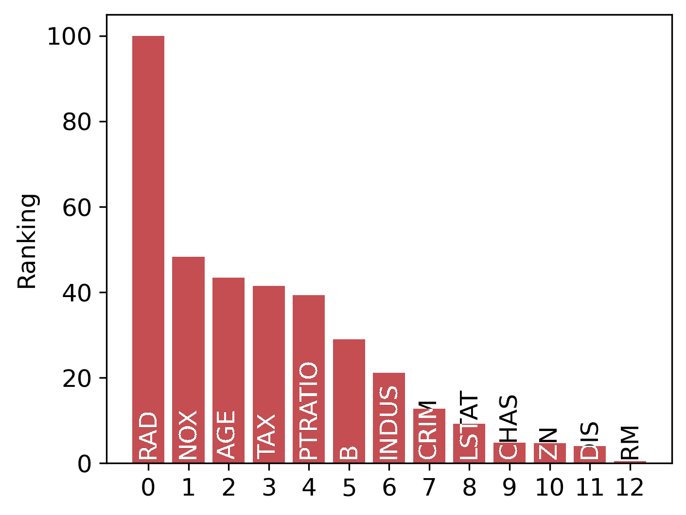
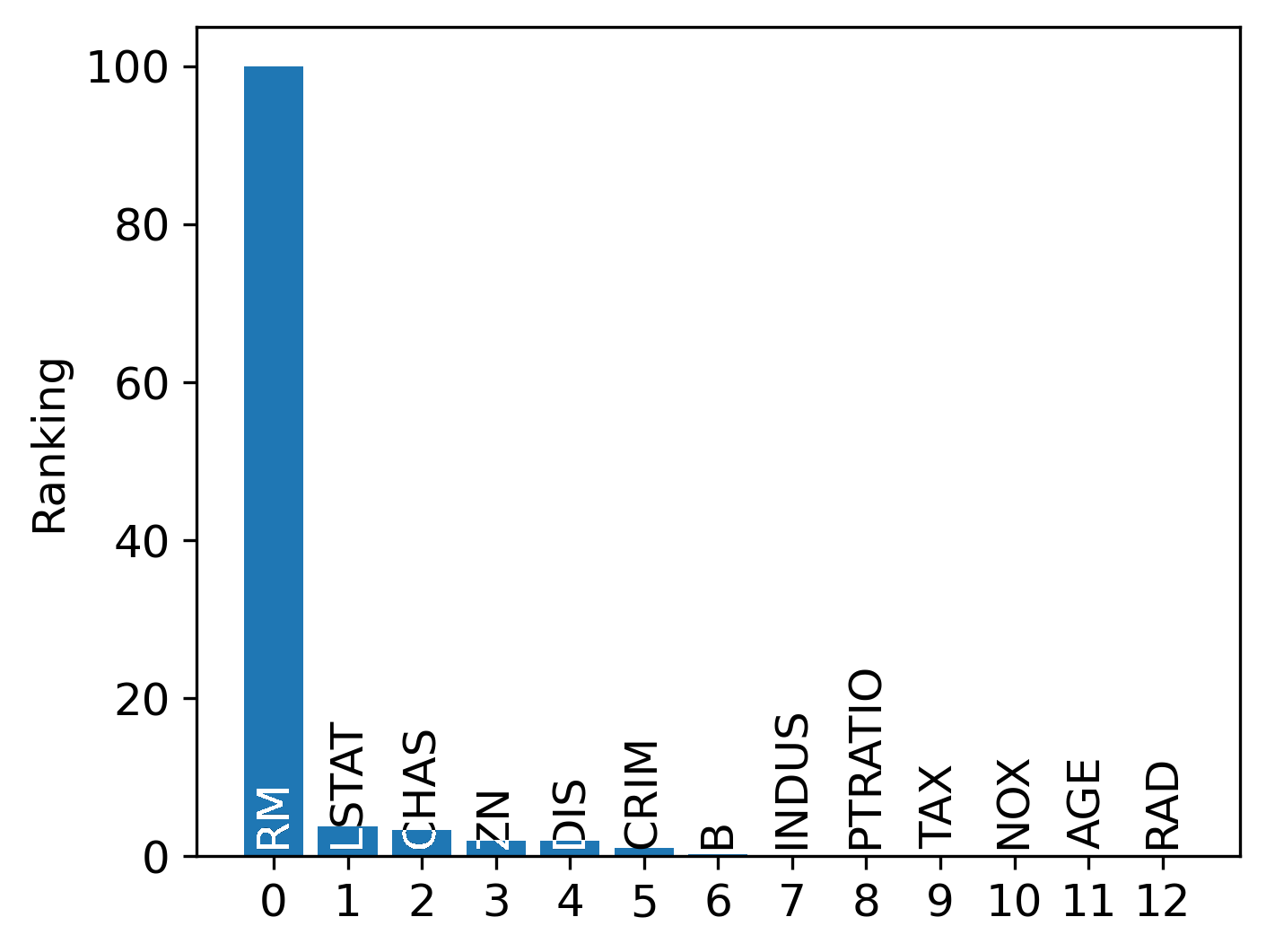
In both cases, the feature model is retrained 250 times and the weight information (weight and variance) retrieved from training iterations are visualized in a weight plot in Supporting Information Fig.1. The feature importance is ranked based on the RVTW and to compare the difference with the effect of the VTF, we applied both methods in the feature set, resulting a feature importance profile and a feature unimportance profile, as depicted in the histogram in Fig.3. The feature importance profile varies as the number of retrain times increasing and becomes stable after some iterations, shown in Supporting Information Fig.4.
IV-A2 Baseline Contribution Factor
Given the results from feature model retraining, an equation system was constructed as described in Eqn.9, where remains unknown. To obtain this parameter, the base model was used to evaluate various settings of the feature set according to the procedure in Supporting Information and the loss change was then used to simulate the relationship between weights and contributions .
Two equation systems of more than 13 equations with 13 unknowns, and more than 30 equations with 30 unknowns were solved with Gaussian reduction algorithm, where the unknowns represent the contribution of each single feature in the feature set. To capture the relationship of the distribution of each feature, the results of the equation system are divided by one of the features’ distribution. Fig.3 (c) presents an overview of the contribution of each feature and detailed contributions are also provided in Supporting Information Fig.5. With the more equations included, the change in the contribution distribution is shown in Supporting Information Fig.6.
IV-A3 Baseline Evaluation
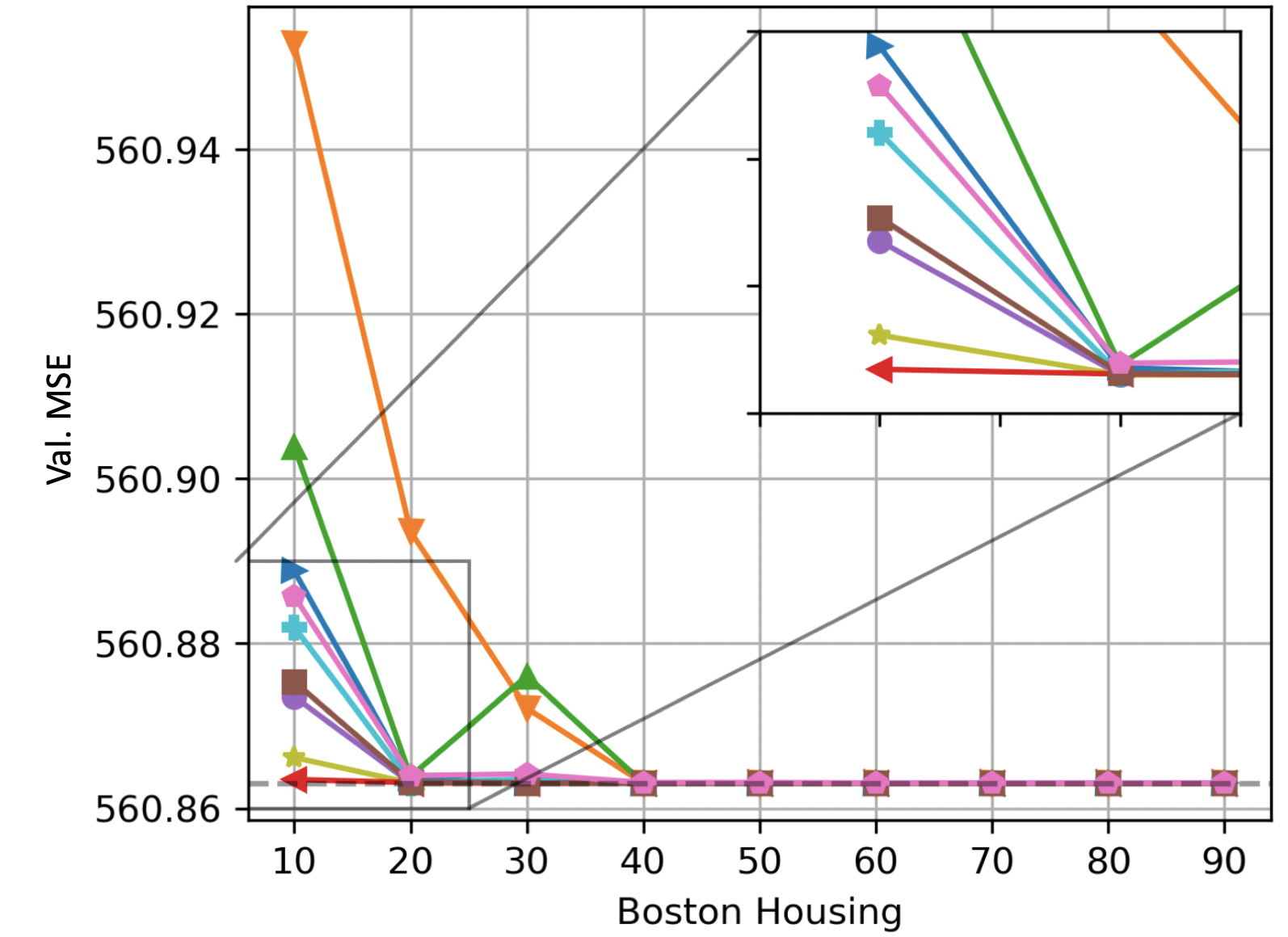
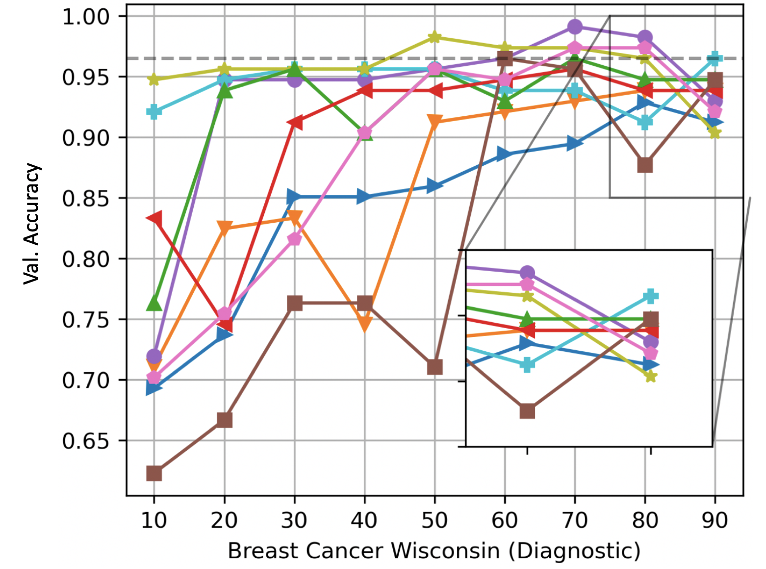
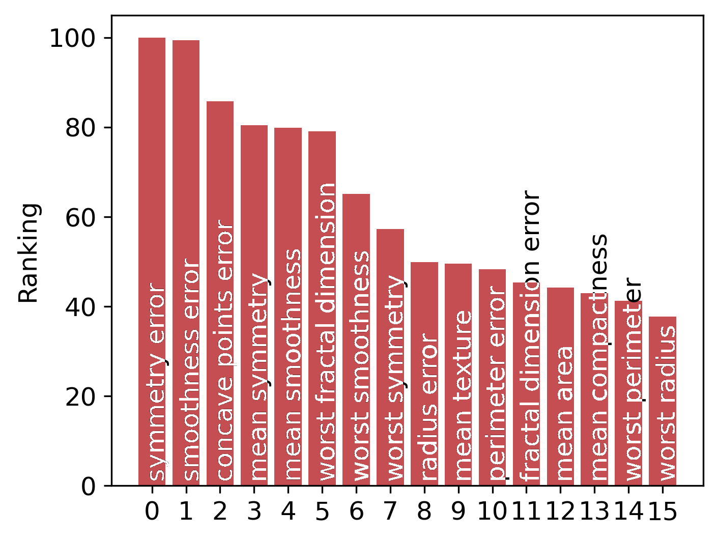
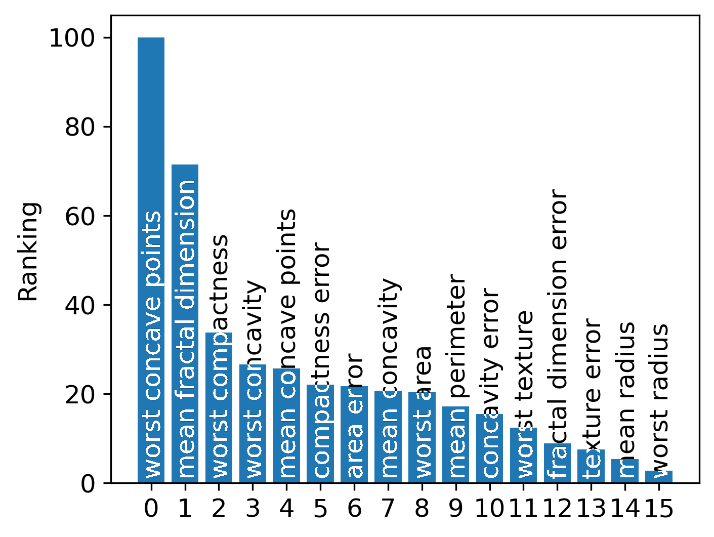
From Table.I, it shows that our feature selection method can achieve similar performance in much shorter time. The permutation method, connection weights, RF, KernelSHAP, Fisher Score, ReliefF and AFS are used as a benchmark to evaluate the performance of the theory applied in the linear regressor. All feature importance profiles are provided in Supporting Information Fig.7. From the importance profile, we can see that LSTAT and RM occurs most among important features in all rankings, and AGE and NOX occurs most among least features in all rankings for Boston Housing Dataset. From Fig.2 (a) we can observe that the model performance drops more with 80% and 90% important features extracted from RVTW and CF than others except RF, while our methods still accurately detect the important features. In the case of 70% important features removed, CF outperforms others and from 60% important features removal, all methods perform similarly. In terms of logistic regression case, mean perimeter, worst area and worst concave points occurs most among important features in all rankings, and symmetry error, worst error and mean fractal dimension occurs most among least features in all rankings. Fig.2 (b) shows that accuracy gaps between baseline and results from RVTW are wider than most methods, while CF performs in average.
V Application
The framework is also applied to widely-used neural networks, convolutional neural network (CNN), recurrent neural network (RNN) and multilayer perceptron (MLP). Training details and network structures are tabulated in Supporting Information Table.10.
V-A Convolutional Neural Network
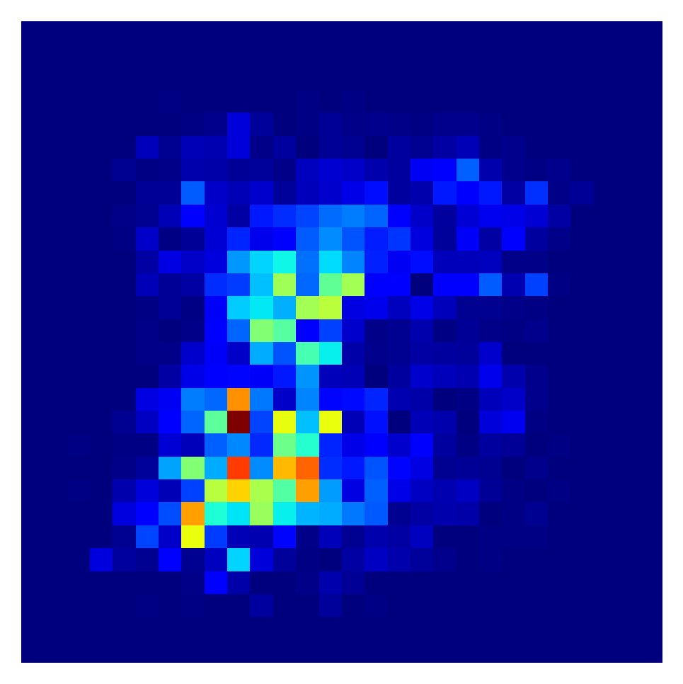
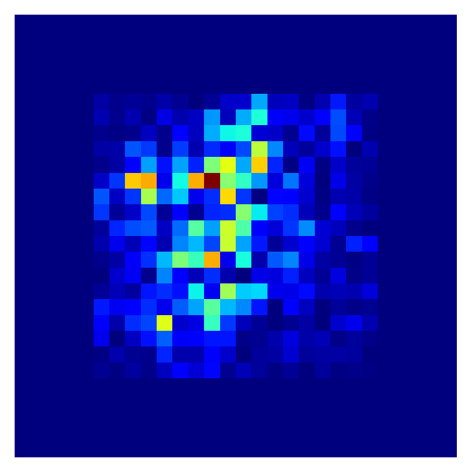
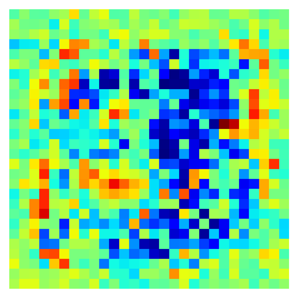
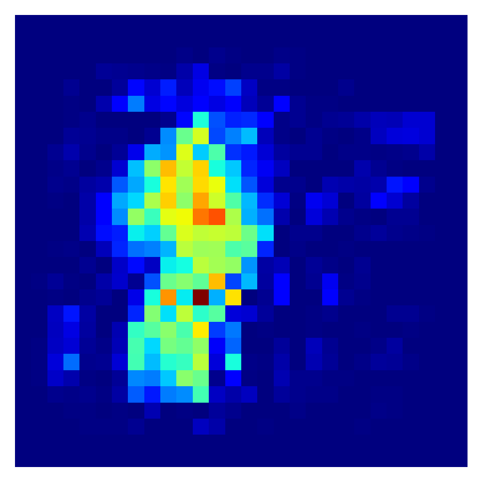
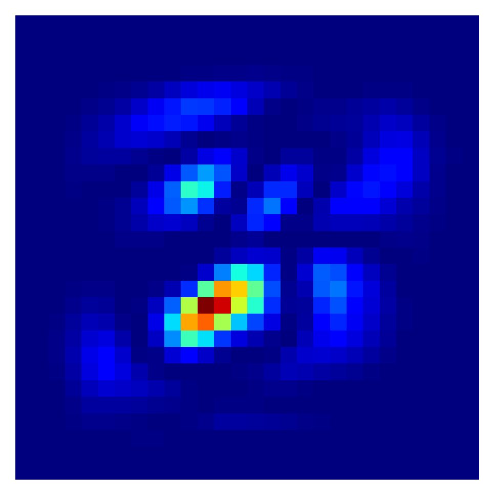
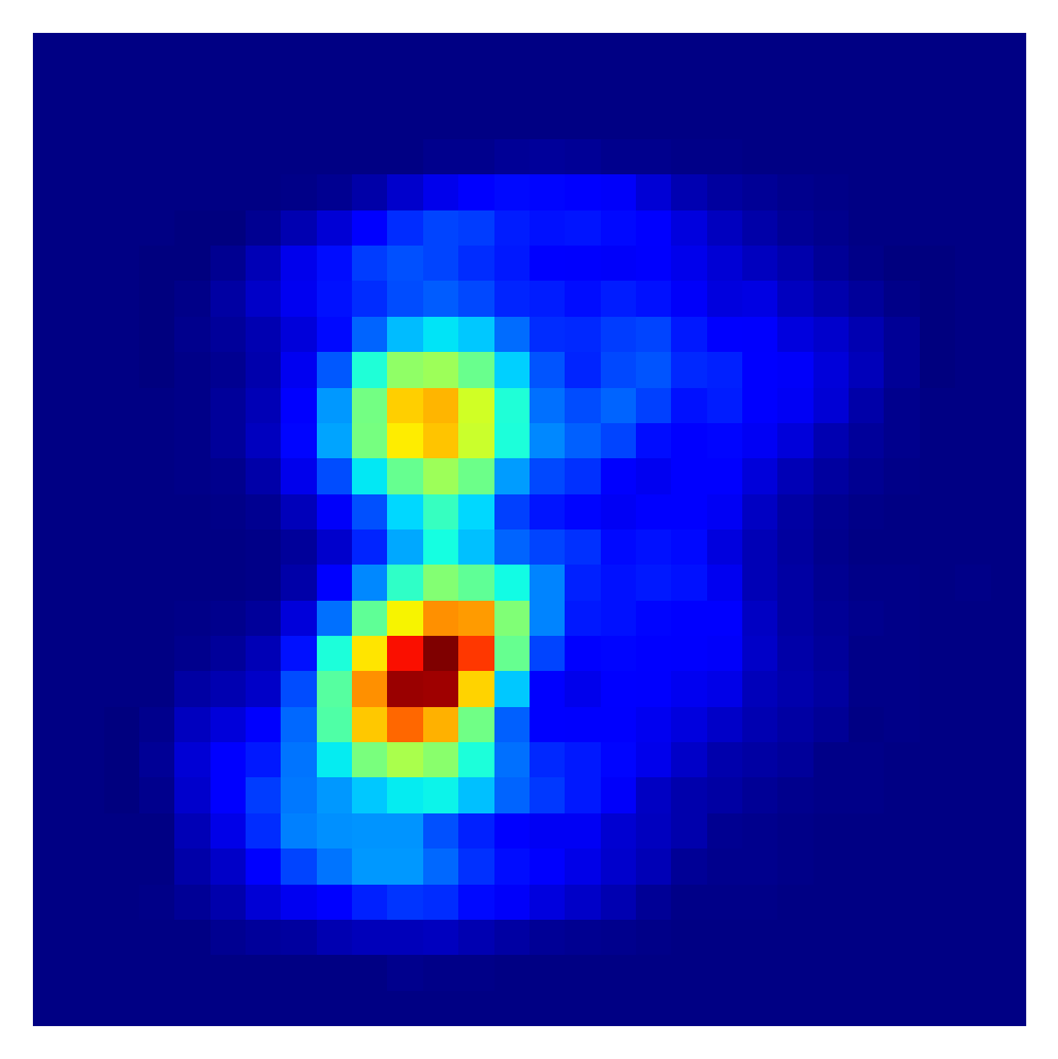
To demonstrate the interpretability of the methods via visual inspection, we employ a CNN to classify the MNIST well-known benchmark dataset [32], focusing on the hard-to-distinguish digits “3” and “8”. The subset is a dataset of 13966 grayscale images, and can be accessed from TensorFlow library [33], with 784 features and 2 classes, where each pixel can be treated as a feature. The base model was first trained for 1000 epochs, achieving 100% accuracy with low loss.
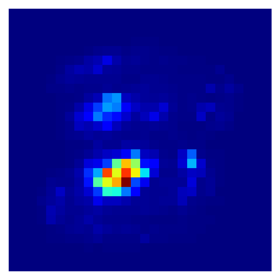
The feature model was trained and optimised using all images to classify the output until the loss achieved the same number as base model. The retraining process was conducted 800 times, which is greater than the number of features (784) needed for the CF. The feature model also achieves the same loss with 100% accuracy. The feature importance is ranked based on RVTW and CF, the pixel importances as shown in Fig.4. Fig.4(c) presents an overview of the contribution of each feature.
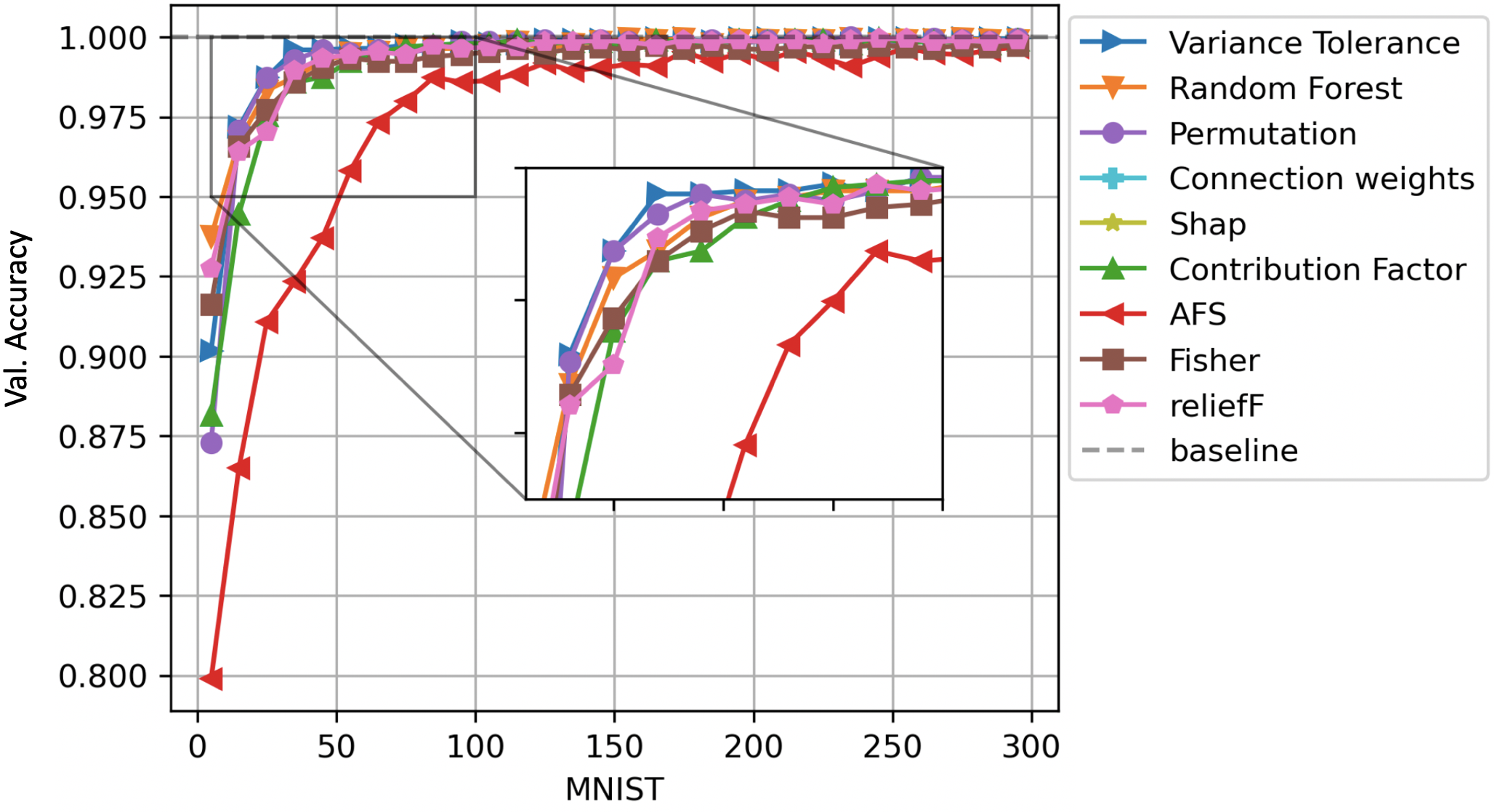
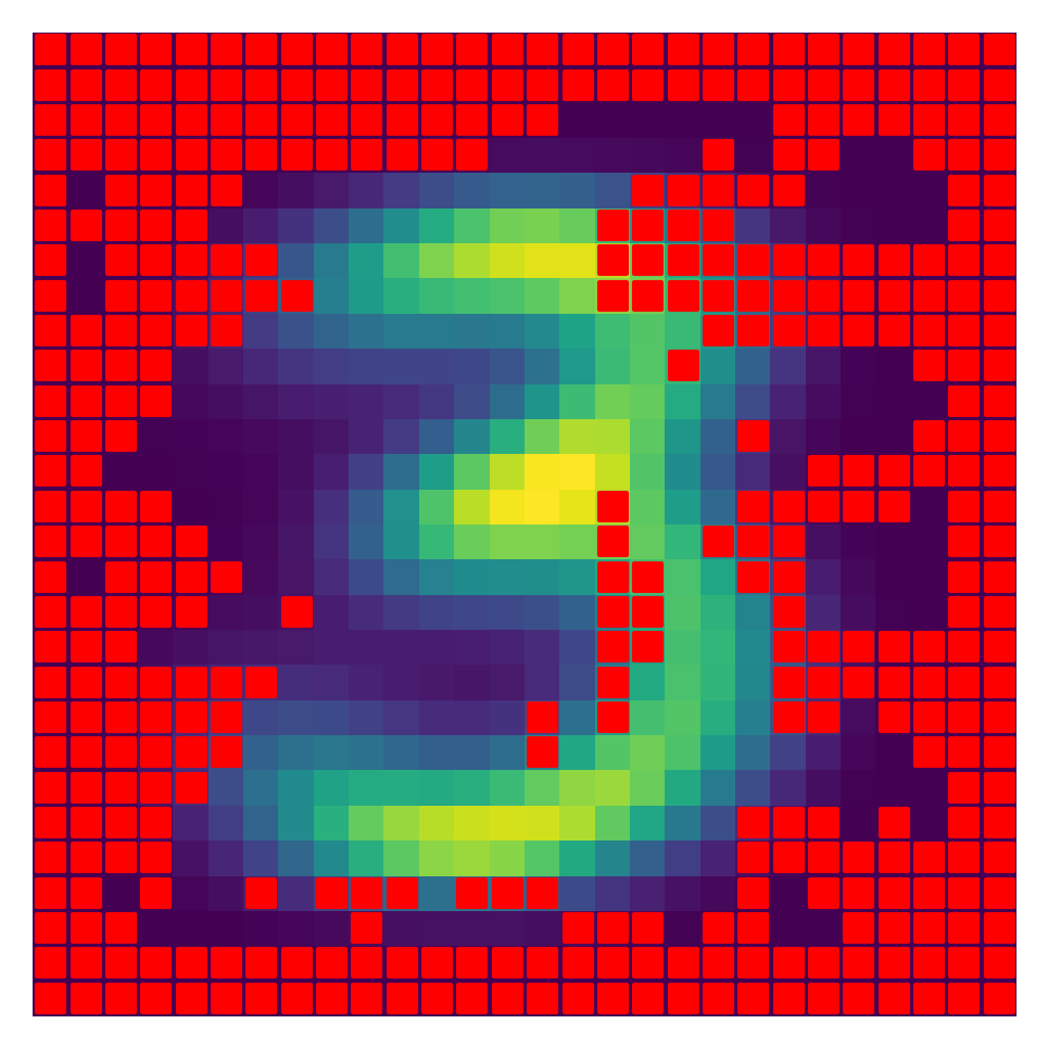
The AFS, Fisher Score, ReliefF, permutation method and RF are used as a benchmark. The permutation method results in a feature importance map after permuting pixels across all images in Fig.4(a). The RF regressor fitted the relationship between 784 features and the class, with 98.89% accuracy, and the feature importance based on Gini impurity is ranked in Fig.4(b). We can see from Fig.4(a-g) that the RVTW and ReliefF produce more interpretable and meaningful maps than other methods for human. From the Fig.2 (c), we can observe that RVTW achieves the best accuracy on almost all feature selection ranges. The CF method yields a map similar to the permutation method. Unimportant pixels are marked Fig.4 (h). Overall, our proposed methods can produce promising outcomes.
V-B Recurrent Neural Network
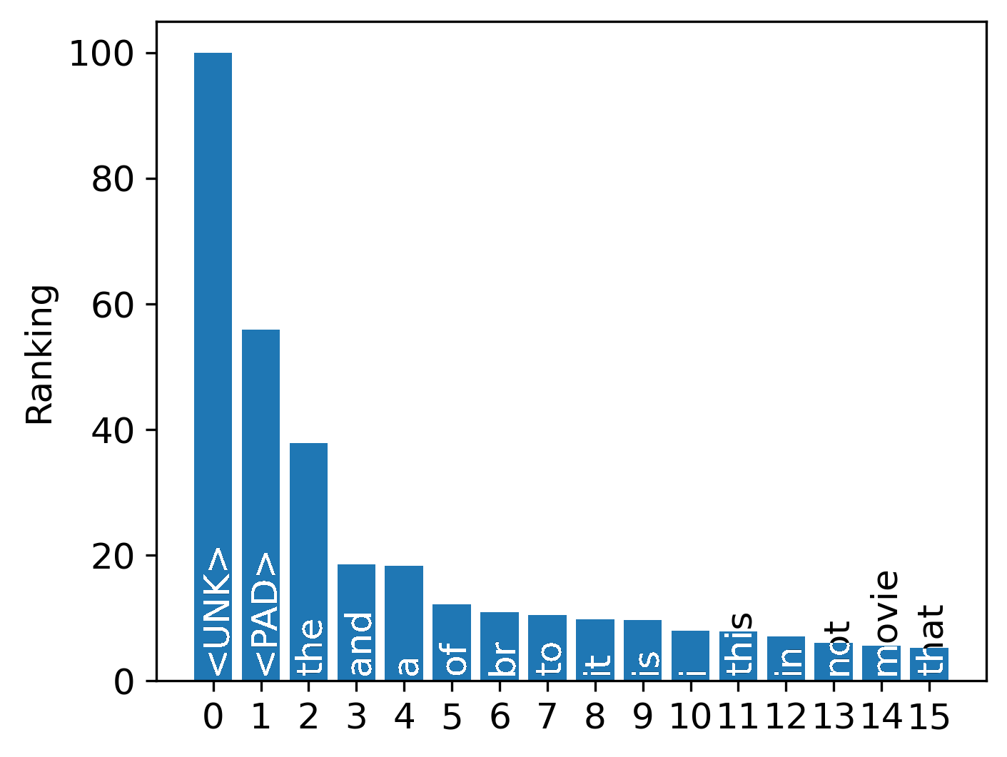
To demonstrate the interpretability of the methods in sentiment analysis, we employ the RVTW and CF in a RNN on IMDB movie reviews [34], to classify the overall review as positive or negative, where each word is considered as a feature. For the purpose of demonstration, the dataset is loaded from TensorFlow library [33], where each review is encoded as a list of integers. For convenience, only the top 2,000 most common words are considered and actual words are indexed from 3. An RNN base model is constructed following the structure and trained for 500 epochs, achieving 88.24% accuracy with low loss.
The feature model was constructed based on the outputs of the base model, however, the length of sentence is fixed and a sentence can’t contain all words. To update the weight of each word in each iteration and rank all words in a library, the mask layer is located between a one-hot layer and an LSTM layer. The feature model was retrained 2000 times since 2000 features were needed to demonstrate the CF method. The feature model also achieves the similar loss with 88% accuracy. The feature importance is ranked and visualised in Fig.5(a-e).
As mentioned above, due to the large scale of the word bank, we constructed an equation system with 2000 unknowns and 2000 equations to demonstrate the success in RNN. The contribution of top 30 words are ranked and shown in Fig.5(c), where is impossible to present all words.
Considering the computing complexity, only permutation method and RF are used as a benchmark to evaluate the performance of the VTF-based methods applied to an RNN. To fit all sentences and rank their feature importance, all sentences are encoded using one-hot format and fitted using a RF regressor based on Gini impurity. The accuracy is 82.94 % results and importances are illustrated in Fig.5(a). By permuting each word in the library in each sentence, the feature importance profile can be obtained according to their loss change, shown in Fig.5(b).
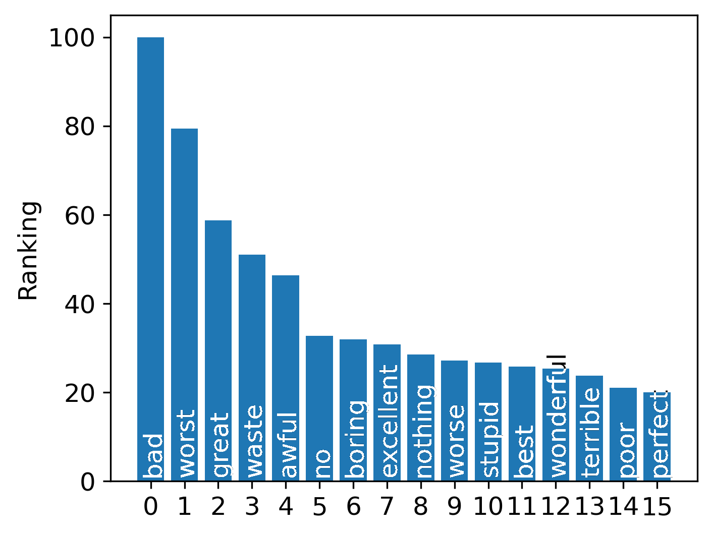
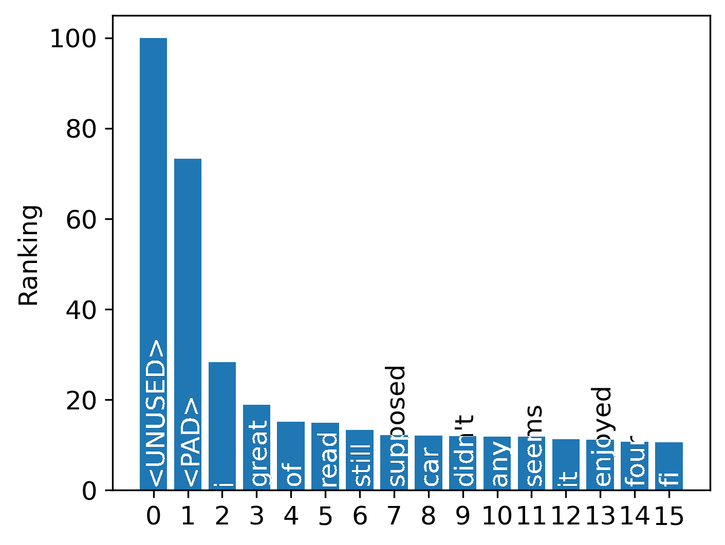
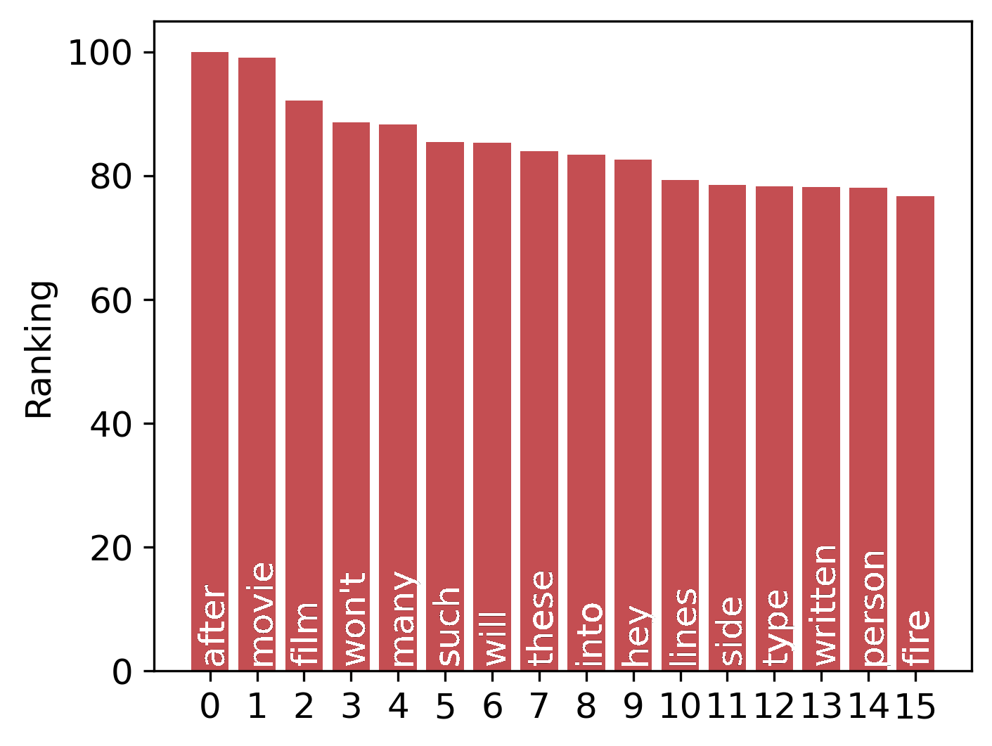
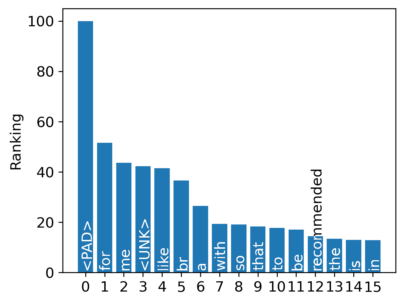
Semantic analysis using RNN is an example showing the feasibility and flexibility of the framework, but when the corpus (each representing a feature) is large, it becomes impractical. Unimportant feature profile from the VTF treats most of the unimportant features equally, so the CF and RVTW capture the most frequently occurring words, like the permutation method, even if some of them are uninformative.
| Linear regression | |||
|---|---|---|---|
| Our method | RFE | Base model | |
| Time complexity | - | ||
| MSE | 3.4014 | 3.4097 | 3.4003 |
| Logistic regression | |||
| Time complexity | - | ||
| Loss | 0.0866 | 0.0834 | 0.0812 |
| Convolutional Neural Network | |||
| Time complexity | - | ||
| Accuracy | 99.76% | - | 100% |
| Recurrent Neural Network | |||
| Time complexity | - | ||
| Accuracy | 87.96% | - | 88% |
V-C Real-world Applications
In this study, we implemented our proposed framework on real-world datasets, tackling two difficult tasks. The first task involved predicting the formation of highly disordered nanoparticles based on their physical properties, while the second task involved predicting the chemical property from aromatic compounds [35]. Further information regarding the datasets and experimental procedures are provided in the subsequent sections.
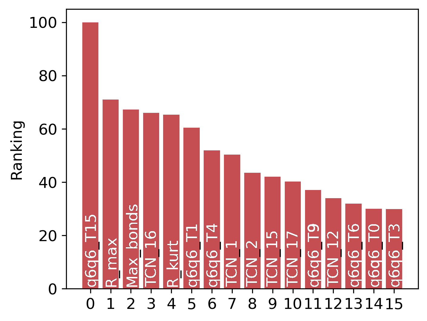
V-C1 Gold Nanoparticles
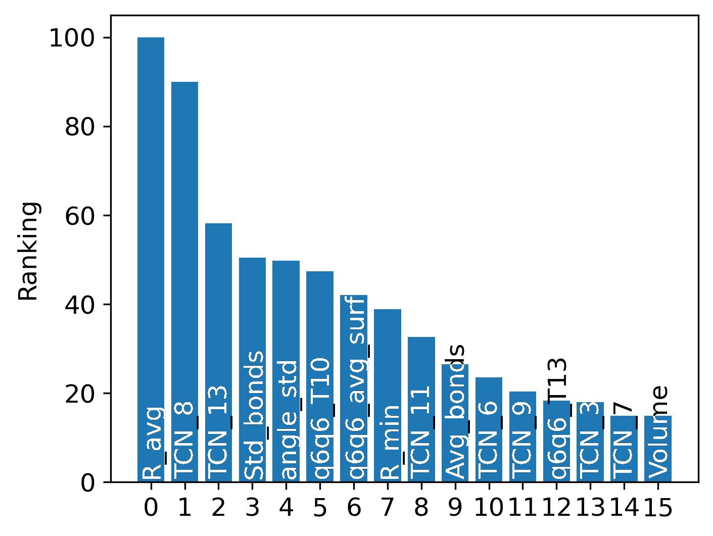
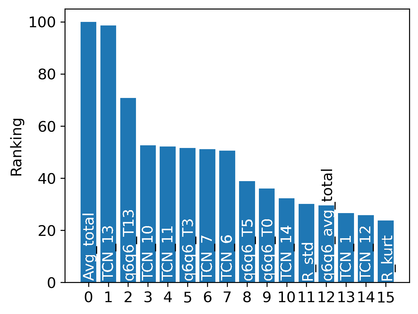
The dataset used for this study contains 4000 gold (Au) nanoparticles generated using molecular dynamics at various temperatures, growth rates and times, which is available online [36]. Atomistic, molecular, topological and crystallographic descriptors are characterised as features and the formation energies are assigned as the target property labels. Based on different types of information about the nanoparticles the features are grouped into 5 different feature sets, referred as Bulk (B), Surface (S), Totals (T), Condensed (C) and Expanded (E). A comprehensive evaluation of different machine learning models on these feature sets has been previously reported [37]. In the present study T feature set is used to train a MLP and all 5 feature sets are used to train individually linear regressors. The model structures are listed in Supporting Information Table.9. A total of 5 linear regressors reproduced the reported LR results [37] in Supporting Information Table.1, while MLP achieved better performance in T set, with a MAE of 0.0282.
According to the number of features, the feature model is retrained from 35 to 150 times. The feature importance is ranked based on the VTF, RVTW and CF, and the feature unimportance and importance maps for the MLP are visualised in Fig.5 (f-h). Feature importance profiles extracted from 5 linear regressors are provided in Supporting Information Fig.8. We can observe our histograms differs from the reported Extra-trees outcomes [37], which is to be expected. Different machine learning models trained on same task lead to different rankings.
V-C2 Chemical Toxicity
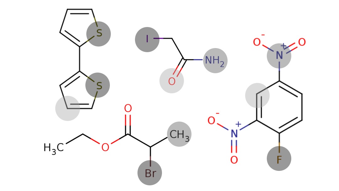
The dataset shows the 50% growth inhibitory concentration of the Tetrahymena pyriformis organism (a protozoan ciliate) when exposed for 40 hours and contains 1793 aromatic compounds. The SMILES2vec model [38] is a mixed CNN-GRU architecture that automatically learns features from SMILES strings [39] to predict chemical properties [40]. The main architecture consists of an embedding layer, convolutional layer with RELU activation and Gated Recurrent Units (GRU). The model is trained for 200 epochs and achieved a faithful validation MSE of 0.31 based on the previous report [35]. The training setting can be found in the Appendix. The explanation mask takes the embedded SMILES representation as input and generates a character-level importance profile. The feature model was trained and optimised until the MSE achieved the same number as base model, or slightly better.
To test the model interpretability, we calculated RVTW and CF in this application. Some SMILES samples are converted to structures for visualizing. In Fig 6, we highlight the important character based on the extracted feature importance profile, darker circles indicating more importance from the mask. From the result, we can observe that the model is more sensitive to atoms from hydrophilic groups, such as F, I, Br and S, deeming them more important. Considering the fact that many halogenated compounds are toxic, these atoms play a critical role in such compounds. The results from data-driven are consistent domain knowledge.
VI Conclusion
In general, the aim of present work is to provide human-readable interpretability to black box models in the Rashomon set by measuring the tolerance of the model to the change of features. The present approach is motivated by linear regression [41] and Shapley values, and the way to accomplish the idea comes from transformer [42], fixing the parameters from the base model and training a feature model. Weights of the mask layer on feature model are completely data-driven feature importances and we proposed two methods based on VTF, RVTW and CF, to endow interpretability at a global level in the Rashomon set, which can be combined with human understanding. More importantly, other possibilities for interpretability still exist. The universality of this approach is demonstrated by deploying in linear regressor, logistic regressor for general cases; CNN for image-related tasks; RNN for semantic analysis and two real-world applications are provided to show the importance and usage of interpretability for physicochemical systems.
Our method is fast and flexible in model selection, feature selection and feature representation, such as visualising individual words and image pixels in the experiments. It can easily make use of any advanced neural networks to be our component-base model in the framework by separating interpretability from models [43], meaning it is not limited to certain models that might lose predictive performance. The model is applicable to all neural networks, irrespective of their performance, however, neural networks with poor performance hold no value. In the language processing case, the random forest classifies the words with accuracy 82.94%, while RNN can achieve 88% accuracy. The feature unimportance profile is not exactly the reverse of important feature profile extracted from VTF, same features ranked at different positions, like AGE and NOX in Fig.3. With more factors taken into consideration, the outcome of the RVFW ranking is different from other feature importance profiles, but top important features are always selected, although their positions vary as different approaches being applied. It is not fair to judge the performance of a ranking over another, as the interpretability is subjective, but if a feature is selected as important by different approaches, it informs the importance of that feature. The performance of feature selection methods based on the result from Fig.2 demonstrate the reliability and accuracy of our methods. CF provides more detailed interpretability for machine learning models by calculating contribution of each feature through solving equation systems. In addition to ranking the feature importance profile, the method also calculates specific contribution values for features. More importantly, the method opens a new field for interpretable methods for further investigation and the potential for directly measuring the impact of ”domain-driven” interventions by researchers.
Several comparative and classic methods are used to provide insights from different perspectives, including model-agnostic methods and model-specific methods: connection weights, random forest, KernelShap, permutation method, AFS, ReliefF and Fisher Score. Olden [13] found that the connection weight approach achieves the best performance for accurately quantifying variable importance among 8 approaches. The performance of the connection weight approach highly depends on the initial weights used for starting the training process [12], whereas the retraining strategy in our method mitigates the dependence on initial weights. Tree-based methods, such as random forests, are interpretable models but fail to deal with linear relationships and are impossible to extend to neural networks, while our new method is extensible to all machine learning methods and data types. Unlike permuting instances for a feature, all instances are perturbed in a constant way to compare the effect of a feature. The two well-accepted ReliefF and Fisher Score have comparably stable performance, but not accurate as RVFW. AFS performed poorly in MNIST setting and the reason might be the choice of CNN.
There are other machine learning models that can theoretically be used to extend to this work, such as support vector machines or Gaussian process models that are widely used in science and technology, and even unsupervised models. Further application to complex models and huge datasets would help address the scalability, but the above experiments demonstrate the general feasibility and opportunities. As the number of features and model layers increase, it is still feasible to re-train the feature models as suggested, but the computational cost rises correspondingly. Mathematically, the time complexity of a forward pass of a trained MLP depends on the input, number of layers and the size of each layer, and the feature model is trainable as long as the base model can be trained. Discovering the specific relationship between the size, complexity and feature model training will be the topic of future work.
References
- [1] T. Hastie, R. Tibshirani, and J. Friedman, “The elements of statistical learning,” Cited on, p. 33, 2009.
- [2] C. Rudin, “Stop explaining black box machine learning models for high stakes decisions and use interpretable models instead,” Nature Machine Intelligence, vol. 1, no. 5, pp. 206–215, 2019.
- [3] F. Doshi-Velez and B. Kim, “Towards a rigorous science of interpretable machine learning,” arXiv preprint arXiv:1702.08608, 2017.
- [4] T. Miller, “Explanation in artificial intelligence: Insights from the social sciences,” Artificial intelligence, vol. 267, pp. 1–38, 2019.
- [5] B. Kim, R. Khanna, and O. O. Koyejo, “Examples are not enough, learn to criticize! criticism for interpretability,” Advances in neural information processing systems, vol. 29, 2016.
- [6] W. Samek, T. Wiegand, and K.-R. Müller, “Explainable artificial intelligence: Understanding, visualizing and interpreting deep learning models,” arXiv preprint arXiv:1708.08296, 2017.
- [7] I. Guyon and A. Elisseeff, “An introduction to variable and feature selection,” Journal of machine learning research, vol. 3, no. Mar, pp. 1157–1182, 2003.
- [8] I. Guyon, J. Weston, S. Barnhill, and V. Vapnik, “Gene selection for cancer classification using support vector machines,” Machine learning, vol. 46, no. 1, pp. 389–422, 2002.
- [9] L. Song, A. Smola, A. Gretton, K. M. Borgwardt, and J. Bedo, “Supervised feature selection via dependence estimation,” in Proceedings of the 24th international conference on Machine learning, 2007, pp. 823–830.
- [10] M. Wojtas and K. Chen, “Feature importance ranking for deep learning,” arXiv preprint arXiv:2010.08973, 2020.
- [11] A. Fisher, C. Rudin, and F. Dominici, “All models are wrong, but many are useful: Learning a variable’s importance by studying an entire class of prediction models simultaneously.” J. Mach. Learn. Res., vol. 20, no. 177, pp. 1–81, 2019.
- [12] O. Ibrahim, “A comparison of methods for assessing the relative importance of input variables in artificial neural networks,” Journal of applied sciences research, vol. 9, no. 11, pp. 5692–5700, 2013.
- [13] J. D. Olden, M. K. Joy, and R. G. Death, “An accurate comparison of methods for quantifying variable importance in artificial neural networks using simulated data,” Ecological modelling, vol. 178, no. 3-4, pp. 389–397, 2004.
- [14] C. Molnar, “A guide for making black box models explainable,” URL: https://christophm. github. io/interpretable-ml-book, 2018.
- [15] X. Liu, X. Wang, and S. Matwin, “Improving the interpretability of deep neural networks with knowledge distillation,” in 2018 IEEE International Conference on Data Mining Workshops (ICDMW). IEEE, 2018, pp. 905–912.
- [16] T. K. Ho, “Random decision forests,” in Proceedings of 3rd international conference on document analysis and recognition, vol. 1. IEEE, 1995, pp. 278–282.
- [17] J. H. Friedman, “Greedy function approximation: a gradient boosting machine,” Annals of statistics, pp. 1189–1232, 2001.
- [18] S. M. Lundberg and S.-I. Lee, “A unified approach to interpreting model predictions,” in Proceedings of the 31st international conference on neural information processing systems, 2017, pp. 4768–4777.
- [19] K. A. Gallagher, Z.-J. Liu, M. Xiao, H. Chen, L. J. Goldstein, D. G. Buerk, A. Nedeau, S. R. Thom, O. C. Velazquez et al., “Diabetic impairments in no-mediated endothelial progenitor cell mobilization and homing are reversed by hyperoxia and sdf-1,” The Journal of clinical investigation, vol. 117, no. 5, pp. 1249–1259, 2007.
- [20] Q. Gu, Z. Li, and J. Han, “Generalized fisher score for feature selection,” arXiv preprint arXiv:1202.3725, 2012.
- [21] M. Robnik-Šikonja and I. Kononenko, “Theoretical and empirical analysis of relieff and rrelieff,” Machine learning, vol. 53, no. 1, pp. 23–69, 2003.
- [22] J. C. Davis and R. J. Sampson, Statistics and data analysis in geology. Wiley New York, 1986, vol. 646.
- [23] J. Tang, S. Alelyani, and H. Liu, “Data classification: algorithms and applications,” Data Mining and Knowledge Discovery Series, pp. 37–64, 2014.
- [24] N. Gui, D. Ge, and Z. Hu, “Afs: An attention-based mechanism for supervised feature selection,” in Proceedings of the AAAI conference on artificial intelligence, vol. 33, 2019, pp. 3705–3713.
- [25] L. Breiman, “Statistical modeling: The two cultures (with comments and a rejoinder by the author),” Statistical science, vol. 16, no. 3, pp. 199–231, 2001.
- [26] J. Dong and C. Rudin, “Exploring the cloud of variable importance for the set of all good models,” Nature Machine Intelligence, vol. 2, no. 12, pp. 810–824, 2020.
- [27] P. W. W. Koh, K.-S. Ang, H. Teo, and P. S. Liang, “On the accuracy of influence functions for measuring group effects,” Advances in neural information processing systems, vol. 32, 2019.
- [28] S. Basu, X. You, and S. Feizi, “On second-order group influence functions for black-box predictions,” in International Conference on Machine Learning. PMLR, 2020, pp. 715–724.
- [29] A. Asuncion and D. Newman, “Uci machine learning repository,” 2007.
- [30] F. Pedregosa, G. Varoquaux, A. Gramfort, V. Michel, B. Thirion, O. Grisel, M. Blondel, P. Prettenhofer, R. Weiss, V. Dubourg, J. Vanderplas, A. Passos, D. Cournapeau, M. Brucher, M. Perrot, and E. Duchesnay, “Scikit-learn: Machine learning in Python,” Journal of Machine Learning Research, vol. 12, pp. 2825–2830, 2011.
- [31] W. H. Wolberg, W. N. Street, and O. L. Mangasarian, “Breast cancer wisconsin (diagnostic) data set,” UCI Machine Learning Repository [http://archive. ics. uci. edu/ml/], 1992.
- [32] L. Deng, “The mnist database of handwritten digit images for machine learning research,” IEEE Signal Processing Magazine, vol. 29, no. 6, pp. 141–142, 2012.
- [33] M. Abadi, A. Agarwal, P. Barham, E. Brevdo, Z. Chen, C. Citro, G. S. Corrado, A. Davis, J. Dean, M. Devin, S. Ghemawat, I. Goodfellow, A. Harp, G. Irving, M. Isard, Y. Jia, R. Jozefowicz, L. Kaiser, M. Kudlur, and …Xiaoqiang Zheng, “TensorFlow: Large-scale machine learning on heterogeneous systems,” 2015, software available from tensorflow.org. [Online]. Available: https://www.tensorflow.org/
- [34] A. Maas, R. E. Daly, P. T. Pham, D. Huang, A. Y. Ng, and C. Potts, “Learning word vectors for sentiment analysis,” in Proceedings of the 49th annual meeting of the association for computational linguistics: Human language technologies, 2011, pp. 142–150.
- [35] A. Karim, V. Riahi, A. Mishra, M. H. Newton, A. Dehzangi, T. Balle, and A. Sattar, “Quantitative toxicity prediction via meta ensembling of multitask deep learning models,” ACS omega, vol. 6, no. 18, pp. 12 306–12 317, 2021.
- [36] Barnard, Amanda; Opletal, George, “Gold Nanoparticle Data Set. v1. CSIRO. Data Collection.” https://doi.org/10.25919/5d395ef9a4291, 2019.
- [37] A. S. Barnard and G. Opletal, “Selecting machine learning models for metallic nanoparticles,” Nano Futures, vol. 4, no. 3, p. 035003, 2020.
- [38] G. B. Goh, N. O. Hodas, and A. Vishnu, “Deep learning for computational chemistry,” Journal of computational chemistry, vol. 38, no. 16, pp. 1291–1307, 2017.
- [39] D. Weininger, “Smiles, a chemical language and information system. 1. introduction to methodology and encoding rules,” Journal of chemical information and computer sciences, vol. 28, no. 1, pp. 31–36, 1988.
- [40] G. B. Goh, N. O. Hodas, C. Siegel, and A. Vishnu, “Smiles2vec: An interpretable general-purpose deep neural network for predicting chemical properties,” arXiv preprint arXiv:1712.02034, 2017.
- [41] I. Goodfellow, Y. Bengio, and A. Courville, “Machine learning basics,” Deep learning, vol. 1, no. 7, pp. 98–164, 2016.
- [42] M. Ji, B. Heo, and S. Park, “Show, attend and distill: Knowledge distillation via attention-based feature matching,” in Proceedings of the AAAI Conference on Artificial Intelligence, vol. 35, 2021, pp. 7945–7952.
- [43] M. T. Ribeiro, S. Singh, and C. Guestrin, ““why should i trust you?” explaining the predictions of any classifier,” in Proceedings of the 22nd ACM SIGKDD international conference on knowledge discovery and data mining, 2016, pp. 1135–1144.