Multi-Sample Training for Neural Image Compression

Abstract

This paper considers the problem of lossy neural image compression (NIC). Current state-of-the-art (sota) methods adopt uniform posterior to approximate quantization noise, and single-sample pathwise estimator to approximate the gradient of evidence lower bound (ELBO). In this paper, we propose to train NIC with multiple-sample importance weighted autoencoder (IWAE) target, which is tighter than ELBO and converges to log likelihood as sample size increases. First, we identify that the uniform posterior of NIC has special properties, which affect the variance and bias of pathwise and score function estimators of the IWAE target. Moreover, we provide insights on a commonly adopted trick in NIC from gradient variance perspective. Based on those analysis, we further propose multiple-sample NIC (MS-NIC), an enhanced IWAE target for NIC. Experimental results demonstrate that it improves sota NIC methods. Our MS-NIC is plug-and-play, and can be easily extended to other neural compression tasks.

1 Introduction

Latent variable-based lossy neural image compression (NIC) has witnessed significant success. The majority of NIC follows the framework proposed by Ballé et al. [2017]: For encoding, the original image $\bm{x}$ is transformed into $\bm{y}$ by the encoder. Then $\bm{y}$ is scalar-quantized into integer $\bm{\bar{y}}$, estimated with an entropy model $p(\bm{\bar{y}})$ and coded. For decoding, $\bm{\bar{y}}$ is transformed back by the decoder to obtain reconstructed $\bm{\bar{x}}$. The optimization target of NIC is R-D cost: $R+\lambda D$. $R$ denotes the bitrate of $\bm{\bar{y}}$, $D$ denotes the distortion between $\bm{x}$ and $\bm{\bar{x}}$, and $\lambda$ denotes the hyper-parameter controlling their trade-off. During training, the quantization $\bm{\bar{y}}=\lfloor\bm{y}\rceil$ is relaxed with $\bm{\tilde{y}}=\bm{y}+\bm{\epsilon}$ to simulate the quantization noise. And $\bm{\epsilon}$ is fully factorized uniform noise $\bm{{\epsilon}}\sim p(\bm{\epsilon})=\prod\mathcal{U}(-\frac{1}{2},+\frac{1}{2})$.

Ballé et al. [2017] further recognises that such training framework is closely related to variational inference. Indeed, the above process can be formulated as a graphic model $\bm{x}\leftarrow\bm{\tilde{y}}$. During encoding, $\bm{x}$ is transformed into variational parameter $\bm{y}$ by inference model (encoder), and $\bm{\tilde{y}}$ is sampled from variational posterior $q(\bm{\tilde{y}}|\bm{x})$, which is a unit unifrom distribution centered in $\bm{y}$. The prior likelihood $p(\bm{\tilde{y}})$ is computed, and $\bm{\tilde{y}}$ is transformed back by the generative model (decoder) to compute the likelihood $p(\bm{x}|\bm{\tilde{y}})$. Under such formulation, the prior is connected to the bitrate, the likelihood is connected to the distortion, and the posterior likelihood is connected to the bits-back bitrate (See Appendix. A.1), which is $0$ in NIC. Finally, the evidence lower bound (ELBO) is the negative $R+\lambda D$ target (Eq. 1). Denote the transform function $\bm{\tilde{y}}(\bm{\epsilon};\phi)=\bm{y}+\bm{\epsilon}$, and sampling $\bm{\tilde{y}}\sim q(\bm{\tilde{y}}|\bm{x})$ is equivalent to transforming $\bm{\epsilon}$ through $\bm{\tilde{y}}(\bm{\epsilon};\phi)$. Then the gradient of ELBO is estimated via pathwise estimator with single-sample Monte Carlo (Eq. 2). This is the same as SGVB-1 [Kingma and Welling, 2013].

$$\begin{array}[]{l}\mathcal{L}=-(R+\lambda D)=\mathbb{E}_{q(\bm{\tilde{y}}|\bm{x})}[\underbrace{\log p(\bm{x}|\bm{\tilde{y}})}_{\textrm{\scriptsize{- distortion}}}+\underbrace{\log p(\bm{\tilde{y}})}_{\textrm{\scriptsize{- rate}}}\underbrace{-\log q(\bm{\tilde{y}}|\bm{x})}_{\textrm{\scriptsize{bits-back rate: 0}}}]\end{array}$$ (1)

$$\begin{array}[]{l}\nabla_{\phi}\mathcal{L}=\mathbb{E}_{p(\bm{\epsilon})}[\nabla_{\phi}(\log\frac{p(\bm{x},\bm{\tilde{y}}(\bm{\epsilon};\phi))}{q(\bm{\tilde{y}}(\bm{\epsilon};\phi)|\bm{x})})]\approx\nabla_{\phi}\log\frac{p(\bm{x},\bm{\tilde{y}}(\bm{\epsilon};\phi))}{q(\bm{\tilde{y}}(\bm{\epsilon};\phi)|\bm{x})}\end{array}$$ (2)

Ballé et al. [2018] further extends this framework into a two-level hierarchical structure, with graphic model $\bm{x}\leftarrow\bm{\tilde{y}}\leftarrow\bm{\tilde{z}}$. The variational posterior is fully factorized uniform distribution $\mathcal{U}(\bm{y}-\frac{1}{2},\bm{y}+\frac{1}{2})\mathcal{U}(\bm{z}-\frac{1}{2},\bm{z}+\frac{1}{2})$ To simulate the quantization noise. And $\bm{y},\bm{z}$ denote outputs of their inference networks.

$$\begin{array}[]{l}\mathcal{L}=\mathbb{E}_{q(\bm{\tilde{y}},\bm{\tilde{z}}|\bm{x})}[\underbrace{\log p(\bm{x}|\bm{\tilde{y}})}_{\textrm{\scriptsize{- distortion}}}+\underbrace{\log p(\bm{\tilde{y}}|\bm{\tilde{z}})+\log p(\bm{\tilde{z}})}_{\textrm{\scriptsize{- rate}}}\underbrace{-\log q(\bm{\tilde{y}}|\bm{x})-\log q(\bm{\tilde{z}}|\bm{\tilde{y}})}_{\textrm{\scriptsize{bits-back rate: 0}}}]\end{array}$$ (3)

The majority of later NIC follows this hierarchical latent framework [Minnen et al., 2018, Cheng et al., 2020]. Some focus on more expressive network architectures [Zhu et al., 2021, Xie et al., 2021], some stress better context models [Minnen and Singh, 2020, He et al., 2021, Guo et al., 2021a], and some emphasize semi-amortization inference [Yang et al., 2020]. However, there is little research on multiple-sample methods, or other techniques for a tighter ELBO.

On the other hand, IWAE [Burda et al., 2016] has been successful in density estimation. Specifically, IWAE considers a multiple-sample lowerbound $\mathcal{L}_{k}$ (Eq. 4), which is tighter than its single-sample counterpart. The benefit of such bound is that the implicit distribution defined by IWAE approaches true posterior as $k$ increases [Cremer et al., 2017]. This suggests that its variational posterior is less likely to collapse to a single mode of true posterior, and the learned representation is richer. The gradient of $\mathcal{L}_{k}$ is computed via pathwise estimator. Denote the exponential ELBO sample as $w_{i}$, its reparameterization as $w(\bm{\epsilon}_{i};\phi)$, and its weight $\tilde{w}_{i}=\frac{w_{i}}{\sum w_{j}}$. Then $\nabla_{\phi}\mathcal{L}_{k}$ has the form of importance weighted sum (Eq. 5).

$$\begin{array}[]{l}\mathcal{L}_{k}=\mathbb{E}_{q(\bm{\tilde{y}}_{1:k}|\bm{x})}[\log\frac{1}{k}\overset{k}{\underset{i}{\sum}}\underbrace{\frac{p(\bm{x},\bm{\tilde{y}}_{i})}{q(\bm{\tilde{y}}_{i}|\bm{x})}}_{w_{i}}]=\mathbb{E}_{p(\bm{\epsilon}_{1:k})}[\log\frac{1}{k}\overset{k}{\underset{i}{\sum}}\underbrace{\frac{p(\bm{x},\bm{\tilde{y}}(\bm{\epsilon}_{i};\phi))}{q(\bm{\tilde{y}}(\bm{\epsilon}_{i};\phi)|\bm{x})}}_{w(\bm{\epsilon}_{i};\phi)}]\end{array}$$ (4)

$$\begin{array}[]{l}\nabla_{\phi}\mathcal{L}_{k}=\mathbb{E}_{p(\bm{\epsilon}_{1:k})}[\overset{k}{\underset{i}{\sum}}\tilde{w}_{i}\nabla_{\phi}\log w(\bm{\epsilon}_{i};\phi)]\approx\overset{k}{\underset{i}{\sum}}\tilde{w}_{i}\nabla_{\phi}\log w(\bm{\epsilon}_{i};\phi)\end{array}$$ (5)

In this paper, we consider the problem of training NIC with multiple-sample IWAE target (Eq. 4), which allows us to learn a richer latent space. First, we recognise that NIC’s factorized uniform variational posterior has impacts on variance and bias properties of gradient estimators. Specifically, we find NIC’s pathwise gradient estimator equivalent to an improved STL estimator [Roeder et al., 2017], which is unbiased even for the IWAE target. However, NIC’s IWAE-DReG estimator [Tucker et al., 2018] has extra bias, which causes performance decay. Moreover, we provide insights on a commonly adopted but little explained trick of training NIC from gradient variance perspective. Based on those analysis and observations, we further propose MS-NIC, a novel improvement of multiple-sample IWAE target for NIC. Experimental results show that it improves sota NIC methods [Ballé et al., 2018, Cheng et al., 2020] and learns richer latent representation. Our method is plug-and-play, and can be extended into neural video compression.

To wrap up, our contributions are as follows:

• We provide insights on the impact of the uniform variational posterior upon gradient estimators, and a commonly adopted but little discussed trick of NIC training from gradient variance perspective.

• We propose multiple-sample neural image compression (MS-NIC). It is a novel enhancement of hierarchical IWAE [Burda et al., 2016] for neural image compression. To the best of our knowledge, we are the first to consider a tighter ELBO for training neural image compression.

• We demonstrate the efficiency of MS-NIC through experimental results on sota NIC methods. Our method is plug-and-play for neural image compression and can be easily applied to neural video compression.

2 Gradient Estimation for Neural Image Compression

The common NIC framework (Eq. 1, Eq 3) adopts fully factorized uniform distribution $q(\bm{\tilde{y}},\bm{\tilde{z}}|\bm{x})=\prod\mathcal{U}(y^{i}-\frac{1}{2},y^{i}+\frac{1}{2})\prod\mathcal{U}(z^{j}-\frac{1}{2},z^{j}+\frac{1}{2})$ to simulate the quantization noise. Such formulation has the following special properties:

• Property I: $q(\bm{\tilde{z}}|\bm{\tilde{y}})$ and $q(\bm{\tilde{y}}|\bm{x})$’s support depends on the parameter.

• Property II: $\log q(\bm{\tilde{z}}|\bm{\tilde{y}})=\log q(\bm{\tilde{y}}|\bm{x})=0$ on their support.

The impacts of these two properties are frequently neglected in previous works, which does not influence the results for single-sample pathwise gradient estimators (a.k.a. reparameterization trick in Kingma and Welling [2013]). In this section, we discuss the impacts of these two properties upon the variance and biasness of gradient estimators. Our analysis is based on single level latent (Eq. 1) instead of hierarchical latent (Eq. 3) to simplify notations.

2.1 Impact on Pathwise Gradient Estimators

First, let’s consider the single-sample case. We can expand the pathwise gradient of ELBO in Eq. 2 into Eq. 6. As indicated in the equation, $\phi$ contributes to $\mathcal{L}$ in two ways. The first way is through the reparametrized $\bm{\tilde{y}}(\bm{\epsilon};\phi)$ (pathwise term), and the other way is through the parameter of $\log q(\bm{\tilde{y}}|\bm{x})$ (parameter score term). Generally, the parameter score term has higher variance than the pathwise term. The STL [Roeder et al., 2017] reduces the gradient by dropping the score. It is unbiased since the dropped term’s expectation $\mathbb{E}_{q(\bm{\tilde{y}}|\bm{x})}[\nabla_{\phi}\log q_{\phi}(\bm{\tilde{y}}|\bm{x})]$ is $0$.

$$\begin{array}[]{l}\nabla_{\phi}\mathcal{L}=\mathbb{E}_{p(\bm{\epsilon})}[\underbrace{\nabla_{\bm{\tilde{y}}}(\log\frac{p(\bm{x}|\bm{\tilde{y}})p(\bm{\tilde{y}})}{q(\bm{\tilde{y}}|\bm{x})})\nabla_{\phi}\bm{\tilde{y}}(\bm{\epsilon};\phi)}_{\textrm{\scriptsize{pathwise term}}}-\underbrace{\nabla_{\phi}\log q_{\phi}(\bm{\tilde{y}}|\bm{x})}_{\textrm{\scriptsize{parameter score term}}}]\end{array}$$ (6)

Now let’s consider the STL estimator of multiple-sample IWAE bound (Eq. 4). As shown in Tucker et al. [2018], the STL estimation of IWAE bound gradient is biased. To reveal the reason, consider expanding the gradient Eq. 5 into partial derivatives as we expand Eq. 2 into Eq. 6. Unlike single-sample case, the dropped parameter score term $\mathbb{E}_{p(\bm{\epsilon}_{1:k})}[\sum\tilde{w}_{i}(-\nabla_{\phi}\log q_{\phi}(\bm{\tilde{y}}|\bm{x}))]$ is no longer $0$ due to the importance weight $\tilde{w}_{i}$. This means that STL loses its unbiasness in general IWAE cases.

Regarding NIC, however, the direct pathwise gradient for IWAE bound is automatically an unbiased STL estimator. Property II means that variational posterior has constant entropy, which further means that the parameter score gradient is $0$. So, NIC’s pathwise gradient of IWAE bound is equvailent to an extended, unbiased STL estimator.

2.2 Impact on Score Function Gradient Estimators

In previous section, we show the bless of NIC’s special properties on pathwise gradient estimators. In this section, we show their curse on score function gradient estimators. Sepcifically, Property I implies that $q(\bm{\tilde{z}}|\bm{\tilde{y}})$ and $q(\bm{\tilde{y}}|\bm{\tilde{x}})$ are not absolute continuous, and hence the score function gradient estimators of those distributions are biased.

For example, consider a univariate random variable $x\sim p_{\theta}(x)=\mathcal{U}(\theta-\frac{1}{2},\theta+\frac{1}{2})$. Our task is to estimate the gradient of a differentiable function $f(x)$. And consider the $\theta$-independent random variable $\epsilon\sim p(\epsilon)=\mathcal{U}(-\frac{1}{2},+\frac{1}{2})$, the transform $x(\epsilon;\theta)=\theta+\epsilon$. Under such conditions, the Monte Carlo estimated pathwise gradient and score function gradient are:

$$\begin{array}[]{l}\textrm{pathwise gradient: }\nabla_{\theta}\mathbb{E}_{p_{\theta}(x)}[f(x)]=\nabla_{\theta}\mathbb{E}_{p(\epsilon)}[f(x(\epsilon;\theta))]\approx\frac{1}{N}\overset{N}{\underset{i}{\sum}}\nabla_{\theta}f(\theta+\epsilon_{i})\end{array}$$ (7)

$$\begin{array}[]{l}\textrm{score function gradient: }\nabla_{\theta}\mathbb{E}_{p_{\theta}(x)}[f(x)]=\mathbb{E}_{p_{\theta}(x)}[\nabla_{\theta}\log p_{\theta}(x)f(x)]=0\end{array}$$ (8)

Eq. 7 does not equal to Eq. 8, and Eq.8 is wrong. The score function gradient is only unbiased when the distribution satisfies the absolute continuity condition of [Mohamed et al., 2020]. This reflects that under the formulation of NIC, the equivalence between the score function gradient (a.k.a. REINFORCE [Williams, 1992]) and pathwise gradient (a.k.a reparameterization trick in [Kingma and Welling, 2013]) no longer holds.

Table 1: Effect of DReG gradient estimator in NIC.

	Sample Size	bpp	MSE	PSNR (db)	R-D cost
Single-sample
Baseline [Ballé et al., 2018]	-	0.5273	32.61	33.28	1.017
Multiple-sample
MS-NIC-MIX(pathwise gradient)	5	0.5259	31.84	33.38	1.003
MS-NIC-MIX(DReG gradient)	5	0.5316	35.09	32.90	1.058

Such equivalence is the cornerstone of many gradient estimators, and IWAE-DReG [Tucker et al., 2018] is one of them. IWAE-DReG is a popular gradient estimator for IWAE target (Eq. 4) as it resolves the vanish of inference network gradient SNR (signal to noise ratio). However, the correctness of IWAE-DReG depends on the equivalence between the score function gradient and pathwise gradient, which does not hold for NIC. Specifically, IWAE-DReG expand the total derivative of IWAE target as Eq. 9 and perform another round of reparameterization on the score function term as Eq. 10 to further reduce the gradient variance. However, Eq. 10 requires the equivalence of pathwise gradient and score function gradient.

$$\nabla_{\phi}\mathbb{E}_{q_{\phi}(\bm{\tilde{y}}_{1:k}|\bm{x})}[\log\frac{1}{k}\sum_{i=1}^{k}w_{i}]=\mathbb{E}_{p(\bm{\epsilon}_{1:k})}[\sum_{i=1}^{k}\underbrace{\frac{w_{i}}{\sum_{j=1}^{k}w_{j}}(-\frac{\partial\log q_{\phi}(\bm{\tilde{y}}_{i}|\bm{x})}{\partial\phi}}_{\textrm{score function term}}+\frac{\partial\log w(\bm{\epsilon}_{i};\phi)}{\partial\bm{\tilde{y}}_{i}}\frac{\partial\bm{\tilde{y}}(\bm{\epsilon}_{i};\phi)}{\partial\phi})]$$ (9)

$$\mathbb{E}_{q(\bm{\tilde{y}}_{i}|\bm{x})}[\frac{w_{i}}{\sum_{j=1}^{k}w_{j}}\frac{\partial\log q_{\phi}(\bm{\tilde{y}}_{i}|\bm{x})}{\partial\phi}]=\mathbb{E}_{p(\bm{\epsilon_{i}})}[\frac{\partial}{\partial\bm{\tilde{y}}_{i}}(\frac{w_{i}}{\sum_{j=1}^{k}w_{j}})\frac{\partial\bm{\tilde{y}}(\bm{\epsilon}_{i};\phi)}{\partial\phi_{i}}]$$ (10)

As we show empirically in Tab. 1, blindly adopting IWAE-DReG estimator for multiple-sample NIC brings evident performance decay. Other than IWAE-DReG, many other graident estimators such as NVIL [Mnih and Gregor, 2014], VIMCO [Mnih and Rezende, 2016] and GDReG [Bauer and Mnih, 2021] do not apply to NIC. They either bring some extra bias or are totally wrong.

2.3 The direct-y Trick in Training NIC

In NIC, we feed deterministic parameter $\bm{y}$ into z inference model instead of noisy samples $\bm{\tilde{y}}$. This implies that $\bm{\tilde{z}}$ is sampled from $q(\bm{\tilde{z}}|\bm{y})$ instead of $q(\bm{\tilde{z}}|\bm{\tilde{y}})$. This trick is initially adopted in Ballé et al. [2018] and followed by most of the subsequent works. However, it is little discussed. In this paper, we refer it to direct-y trick. Yang et al. [2020] observes that feeding $\bm{\tilde{y}}$ instead of $\bm{y}$ causes severe performance decay. We confirm this result in Tab. 2. Thus, direct-y trick is essential to train hierarchical NIC.

Table 2: Effects of direct-y on R-D performance. 2-level VAE is equivalent to Ballé et al. [2018] without direct-y.

	bpp	MSE	PSNR	R-D cost
2-level VAE	0.9968	33.08	33.22	1.493
[Ballé et al., 2018]	0.5273	32.61	33.28	1.017

Table 3: Effects of direct-y on gradient SNR of different parts of the model. 2-level VAE is equivalent to Ballé et al. [2018] without direct-y. "early" is $5\times 10^{4}$ iterations, "mid" is $5\times 10^{5}$ iterations and "late" is $1\times 10^{6}$ iterations. "infer" is the abbreviation for "inference model", and "gen" is the abbreviation for "generative model".

		gradient SNR of #
Iteration	Method	y infer	y gen	z infer	z gen	z prior
early	2-level VAE	2.287	0.5343	0.3419	0.4099	0.9991
	Ballé et al. [2018]	2.174	0.5179	0.5341	0.3813	1.069
mid	2-level VAE	1.350	0.4793	0.2414	0.3583	0.8861
	Ballé et al. [2018]	1.334	0.4813	0.4879	0.3761	0.9693
late	2-level VAE	1.217	0.4746	0.2863	0.3439	0.8691
	Ballé et al. [2018]	1.206	0.4763	0.5506	0.3707	0.9339

One explanation is to view $q(\bm{\tilde{z}}|\bm{y})$ as $q(\bm{\tilde{z}}|\bm{x})$, and $q(\bm{\tilde{y}},\bm{\tilde{z}}|\bm{\tilde{x}})$ factorized as $q(\bm{\tilde{y}}|\bm{x})q(\bm{\tilde{z}}|\bm{x})$ (See Fig.1 (a)-(c)). A similar trick of feeding mean parameter can be traced back to the Helmholtz machine [Dayan et al., 1995]. However, this provides a rationale why direct-y is fine to be adopted but does not explain why samping $\bm{\tilde{z}}$ from $q(\bm{\tilde{z}}|\bm{\tilde{y}})$ fails. We provide an alternative explanation from the gradient variance perspective. Specifically, $q(\bm{\tilde{z}}|\bm{\tilde{y}})$ has two stochastic arguments that could cause high variance in the gradient of z inference model, and make its convergence difficult. To verify this, we follow Rainforth et al. [2018] to compare the gradient SNR, which is the absolute value of the empirical mean divided by standard deviation. We trace the gradient SNR during different training stages as model converges (See Sec. 5.1 for detailed setups).

As demonstrated in Tab. 3, the gradient SNR of z inference model of standard 2-level VAE (without direct y) is indeed significantly lower than Ballé et al. [2018] (with direct y) during all 3 stage of training. This result reveals that the z inference model is more difficult to train without direct-y. And such difficulty could be the source of the failure of NIC without direct-y trick.

3 Multiple-sample Neural Image Compression

In this section, we consider the multiple-sample approach based on the 2-level hierarchical framework by Ballé et al. [2018], which is the de facto NIC architecture adopted by many sota methods. To simplify notations, $\log q(\bm{\tilde{z}}|\bm{\tilde{y}})$ and $\log q(\bm{\tilde{y}}|\bm{x})$ in ELBO are omitted as they are $0$.

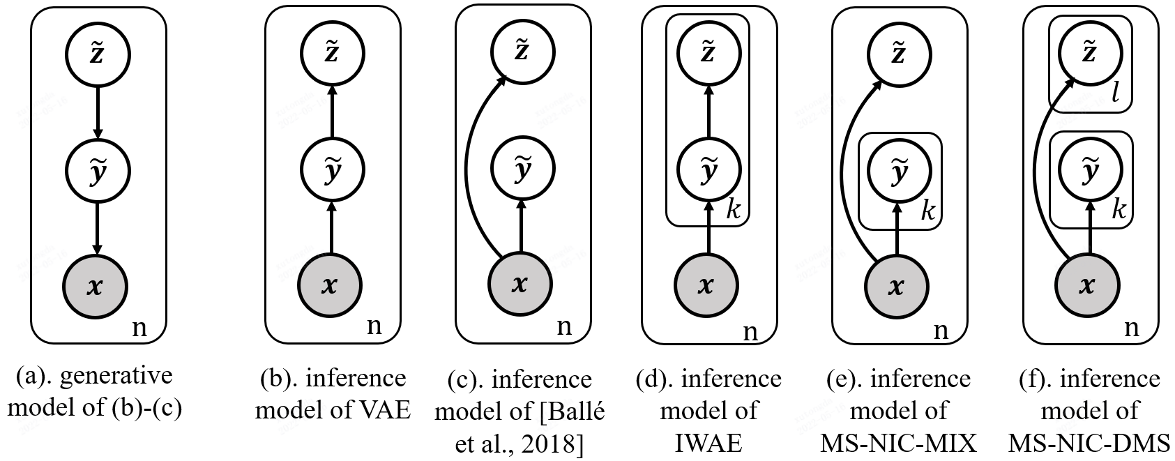
Figure 1: The plate notation of different NIC methods. $\bm{x}$ is the observed image, $\bm{\tilde{y}}$ and $\bm{\tilde{z}}$ are latent. The inference models show how we sample from variational posterior duing training. $n$ is the number of data points in dataset, $k,l$ is the sample size of multiple-sample approaches. The generative model of (b), (c) is (a). The generative model of (d)-(f) is shown in Appendix. A.2. For clarity, we omit the parameters.

First, let’s consider directly applying 2-level IWAE to NIC without direct-y trick (See Fig. 1 (d)). Regarding a $k$ sample IWAE, we first compute parameter $\bm{y}$ of $q(\bm{\tilde{y}}|\bm{x})$ and sample $\bm{\tilde{y}}_{1:k}$ from it. Then, we compute parameter $\bm{z}_{1:k}$ of $q(\bm{\tilde{z}}_{1:k}|\bm{\tilde{y}}_{1:k})$ and samples $\bm{\tilde{z}}_{1:k}$ from it. Afterward, $\bm{\tilde{y}}_{1:k}$ and $\bm{\tilde{z}}_{1:k}$ are fed into the generative model and compute $w_{1:k}$. Finally, we follow Eq 5 to compute the gradient and update parameters. In fact, this is the standard 2-level IWAE in the original IWAE paper.

However, the vanilla 2-level IWAE becomes a problem for NIC with direct-y trick. Concerning a $k$ sample IWAE, we sample $\bm{\tilde{y}}_{1:k}$ from $q(\bm{\tilde{y}}|x)$. Due to the direct-y trick, we feed $\bm{y}$ instead of $\bm{\tilde{y}}_{1:k}$ into z inference network, and our $q(\bm{\tilde{z}}|\bm{y})$ has only one parameter $\bm{z}$ other than $k$ parameter $\bm{z}_{1:k}$. If we follow the 2-level IWAE approach, only one sample $\bm{\tilde{z}}$ is obtained, and $w_{1:k}$ can not be computed. One method is to limit the multiple-sample part to $\bm{\tilde{y}}$ related term only and optimize other parts via single-sample SGVB-1, which produces our MS-NIC-MIX (See Fig 1 (e)). Another method is to sample another $l$ samples of $\bm{\tilde{z}}_{j}$ from $q(\bm{\tilde{z}}|\bm{y})$ and nest it with MS-NIC-MIX, which generates our MS-NIC-DMS (See Fig 1 (f)).

3.1 MS-NIC-MIX: Multiple-sample NIC with Mixture

One way to optimize multiple-sample IWAE target of NIC with direct-y trick is to sample $\bm{\tilde{y}}$ $k$ times to obtain $\bm{\tilde{y}}_{1:k}$ and $\bm{\tilde{z}}$ only $1$ time. Then we perform $k$ sample log mean of $p(\bm{x}|\bm{\tilde{y}}_{i})p(\bm{\tilde{y}}_{i}|\bm{\tilde{z}})$ to obtain a multiple-sample estimated $\log p(\bm{x}|\bm{\tilde{z}})$, add it with single-sample $\log p(\bm{\tilde{z}})$. This brings a $\mathcal{L}^{MIX}_{k}$ with the form of a mixture of 1-level VAE and 1-level IWAE ELBO:

$$\begin{array}[]{l}\mathcal{L}_{k}^{MIX}=\mathbb{E}_{q_{\phi}(\bm{\tilde{z}}|\bm{x})}[\mathbb{E}_{q_{\phi}(\bm{\tilde{y}}_{1:k}|\bm{x})}[\log\frac{1}{k}\overset{k}{\underset{i}{\sum}}p(\bm{x}|\bm{\tilde{y}}_{i})p(\bm{\tilde{y}}_{i}|\bm{\tilde{z}})|\bm{\tilde{z}}]+\log p(\bm{\tilde{z}})]\end{array}$$ (11)

Moreover, $\mathcal{L}^{MIX}_{k}$ is a reasonably preferable target over ELBO as it satisfies the following properties (See Appendix. A.3 for proof):

1. $\log p(x)\geq\mathcal{L}^{MIX}_{k}$

2. $\mathcal{L}^{MIX}_{k}\geq\mathcal{L}^{MIX}_{m}$ for $k\geq m$

Although $\mathcal{L}^{MIX}_{k}$ does not converge to true $\log p(\bm{x})$ as $k$ grows, it is still a lower bound of $\log p(\bm{x})$ and tighter than ELBO (as $\mathcal{L}^{MIX}_{1}=$ ELBO). Its gradient can be computed via pathwise estimator. Denote the per-sample integrand $p(\bm{x}|\bm{\tilde{y}}_{i})p(\bm{\tilde{y_{i}}}|\bm{\tilde{z}})$ as $w^{MIX}_{i}$, and its relative weight as $\tilde{w}^{MIX}_{i}$, then the gradient $\nabla_{\phi}\mathcal{L}_{k}^{MIX}$ can be estimated as Eq. 13.

$$\begin{array}[]{l}\mathcal{L}_{k}^{MIX}=\mathbb{E}_{p(\bm{\epsilon}^{y}_{1:k},\bm{\epsilon}^{z})}[\log\frac{1}{k}\overset{k}{\underset{i}{\sum}}p(\bm{x}|\bm{\tilde{y}}(\bm{\epsilon}^{y}_{i};\phi))p(\bm{\tilde{y}}(\bm{\epsilon}^{y}_{i};\phi)|\bm{\tilde{z}}(\bm{\epsilon}^{z};\phi))+\log p(\bm{\tilde{z}}(\bm{\epsilon}^{z};\phi))]\\ \hskip 30.00005pt\approx\log\frac{1}{k}\overset{k}{\underset{i}{\sum}}\underbrace{p(\bm{x}|\bm{\tilde{y}}(\bm{\epsilon}^{y}_{i};\phi))p(\bm{\tilde{y}}(\bm{\epsilon}^{y}_{i};\phi)|\bm{\tilde{z}}(\bm{\epsilon}^{z};\phi))}_{w^{MIX}(\bm{\epsilon}_{1:k}^{y},\bm{\epsilon}^{z};\phi)}+\log p(\bm{\tilde{z}}(\bm{\epsilon}^{z};\phi))\par\end{array}$$ (12)

$$\begin{array}[]{l}\nabla_{\phi}\mathcal{L}_{k}^{MIX}\approx\overset{k}{\underset{i}{\sum}}\tilde{w}_{i}^{MIX}\nabla_{\phi}\log w^{MIX}(\bm{\epsilon}_{1:k}^{y},\bm{\epsilon}^{z};\phi)+\nabla_{\phi}\log p(\bm{\tilde{z}}(\bm{\epsilon}^{z};\phi))\end{array}$$ (13)

Another way to understand MS-NIC-MIX is to view the y inference/generative model as a single level IWAE, and the z inference/generative model as a large prior of $\bm{\tilde{y}}$ which is optimized via SGVB-1. This perspective is often taken by works in NIC context model [Minnen et al., 2018, He et al., 2021], as the context model of NIC is often limited to $\bm{\tilde{y}}$.

3.2 MS-NIC-DMS: Multiple-sample NIC with Double Multiple Sampling

An intuitive improvement over MS-NIC-MIX is to add another round of multiple-sample over $\bm{\tilde{z}}$. Specifically, we sample $\bm{\tilde{z}}$ $l$ times, nest it with $\mathcal{L}^{MIX}_{k}$ to obtain $\mathcal{L}_{k,l}^{DMS}$:

$$\begin{array}[]{l}\mathcal{L}_{k,l}^{DMS}=\mathbb{E}_{q_{\phi}(\bm{\tilde{z}}_{1:l}|\bm{x})}[\log\frac{1}{l}\overset{l}{\underset{j}{\sum}}\exp{(\mathbb{E}_{q_{\phi}(\bm{\tilde{y}}_{1:k}|\bm{x})}[\log\frac{1}{k}\overset{k}{\underset{i}{\sum}}p(\bm{x}|\bm{\tilde{y}}_{i})p(\bm{\tilde{y}}_{i}|\bm{\tilde{z}}_{j})|\bm{\tilde{z}}_{j}])}p(\bm{\tilde{z}}_{j})]\end{array}$$ (14)

And we name it MS-NIC-DMS as it adopts multiple sampling twice. Moreover, $\mathcal{L}_{k,l}^{DMS}$ is a reasonably better target for optimizaion over ELBO and $\mathcal{L}_{k}^{MIX}$, as it satisfies the following properties (See proof in Appendix. A.3):

1. $\log p(\bm{x})\geq\mathcal{L}^{DMS}_{k,l}$

2. $\mathcal{L}^{DMS}_{k,l}\geq\mathcal{L}^{DMS}_{m,n}$ for $k\geq m,l\geq n$

3. $\mathcal{L}^{DMS}_{k,l}\geq\mathcal{L}^{MIX}_{k}$

4. $\mathcal{L}^{DMS}_{k,l}\rightarrow\log p(\bm{x})$ as $k,l\rightarrow\infty$, under the assumption that $\log\frac{p(\bm{x}|\bm{\tilde{y}}_{i})p(\bm{\tilde{y}}_{i}|\bm{\tilde{z}}_{j})}{q(\bm{\tilde{y}}_{i}|\bm{x})}$ and $\log\frac{p(\bm{x}|\bm{\tilde{z}}_{j})p(\bm{\tilde{z}}_{j})}{q(\bm{\tilde{z}}_{j}|\bm{x})}$ are bounded.

In other words, the target $\mathcal{L}_{k,l}^{DMS}$ is a lowerbound of $\log p(\bm{x})$, converging to $\log p(\bm{x})$ as $k,l\rightarrow\infty$, tighter than $\mathcal{L}_{k}^{MIX}$ and tighter than ELBO (as $\mathcal{L}^{DMS}_{1,1}=$ ELBO). However, its Monte Carlo estimation is biased due to the nested transformation and expectation. Empirically, we find that directly adopting biased pathwise estimator works fine. And its gradient can be estimated by pathwise estimator similar to original IWAE target (See Eq. 5).

$$\begin{array}[]{l}\mathcal{L}_{k,l}^{DMS}=\mathbb{E}_{q(\bm{\epsilon}^{z}_{1:l})}[\log\frac{1}{l}\overset{l}{\underset{j}{\sum}}\exp(\mathbb{E}_{q(\bm{\epsilon}^{y}_{k:l})}[\log\frac{1}{k}\overset{k}{\underset{i}{\sum}}p(\bm{x}|\bm{\tilde{y}}(\bm{\epsilon}^{y}_{i};\phi))p(\bm{\tilde{y}}(\bm{\epsilon}^{y}_{i};\phi)|\bm{\tilde{z}}(\bm{\epsilon}^{z}_{j};\phi))])p(\bm{\tilde{z}}(\bm{\epsilon}^{z}_{j};\phi))]\\ \hskip 30.00005pt\approx\log\frac{1}{l}\overset{l}{\underset{j}{\sum}}\frac{1}{k}\overset{k}{\underset{i}{\sum}}\underbrace{p(\bm{x}|\bm{\tilde{y}}(\bm{\epsilon}^{y}_{i};\phi))p(\bm{\tilde{y}}(\bm{\epsilon}^{y}_{i};\phi)|\bm{\tilde{z}}(\bm{\epsilon}^{z}_{j};\phi))p(\bm{\tilde{z}}(\bm{\epsilon}^{z}_{j};\phi))}_{w^{DMS}(\bm{\epsilon}_{1:k}^{y},\bm{\epsilon}_{1:l}^{z};\phi)}\end{array}$$ (15)

Another interpretation of MS-NIC-DMS is to view it as a multiple level IWAE with repeated local samples. The $\mathcal{L}_{k,l}^{DMS}$ Monte Carlo pathwise estimator has the form of IWAE with $k\times l$ samples. However, there are multiple repeated samples that contain the same $\bm{\tilde{y}}_{i}$ and $\bm{\tilde{z}}_{j}$. For example, the samples $w^{IWAE}_{1:6}$ of 2 level IWAE with sample size 6 look like Eq. 16. While the samples $w^{DMS}_{1:2,1:3}$ of MS-NIC-DMS with $2\times 3$ samples look like Eq. 17. We can see that in IWAE, we have 6 pairs of independently sampled $\bm{\tilde{y}}$ and $\bm{\tilde{z}}$, while in MS-NIC-DMS, we have 2 independent $\bm{\tilde{y}}$ and 3 independent $\bm{\tilde{z}}$, they are paired to generate 6 samples in total. Note that this is only applicable to NIC as $\bm{\tilde{y}}$ and $\bm{\tilde{z}}$ are conditionally independent given $\bm{\tilde{x}}$ due to direct-y trick.

$$\begin{array}[]{l}{w^{IWAE}_{1:6}}=\{p(\bm{x}|\bm{\tilde{y}}_{1})p(\bm{\tilde{y}}_{1}|\bm{\tilde{z}}_{1})p(\bm{\tilde{z}}_{1}),\\ \hskip 50.00008ptp(\bm{x}|\bm{\tilde{y}}_{2})p(\bm{\tilde{y}}_{2}|\bm{\tilde{z}}_{2})p(\bm{\tilde{z}}_{2}),\\ \hskip 50.00008ptp(\bm{x}|\bm{\tilde{y}}_{3})p(\bm{\tilde{y}}_{3}|\bm{\tilde{z}}_{3})p(\bm{\tilde{z}}_{3}),\\ \hskip 50.00008ptp(\bm{x}|\bm{\tilde{y}}_{4})p(\bm{\tilde{y}}_{4}|\bm{\tilde{z}}_{4})p(\bm{\tilde{z}}_{4}),\\ \hskip 50.00008ptp(\bm{x}|\bm{\tilde{y}}_{5})p(\bm{\tilde{y}}_{5}|\bm{\tilde{z}}_{5})p(\bm{\tilde{z}}_{5}),\\ \hskip 50.00008ptp(\bm{x}|\bm{\tilde{y}}_{6})p(\bm{\tilde{y}}_{6}|\bm{\tilde{z}}_{6})p(\bm{\tilde{z}}_{6})\}\end{array}$$ (16)

$$\begin{array}[]{l}{w^{DMS}_{1:2,1:3}}=\{p(\bm{x}|\bm{\tilde{y}}_{1})p(\bm{\tilde{y}}_{1}|\bm{\tilde{z}}_{1})p(\bm{\tilde{z}}_{1}),\\ \hskip 48.00009ptp(\bm{x}|\bm{\tilde{y}}_{1})p(\bm{\tilde{y}}_{1}|\bm{\tilde{z}}_{2})p(\bm{\tilde{z}}_{2}),\\ \hskip 48.00009ptp(\bm{x}|\bm{\tilde{y}}_{1})p(\bm{\tilde{y}}_{1}|\bm{\tilde{z}}_{3})p(\bm{\tilde{z}}_{3}),\\ \hskip 48.00009ptp(\bm{x}|\bm{\tilde{y}}_{2})p(\bm{\tilde{y}}_{2}|\bm{\tilde{z}}_{1})p(\bm{\tilde{z}}_{1}),\\ \hskip 48.00009ptp(\bm{x}|\bm{\tilde{y}}_{2})p(\bm{\tilde{y}}_{2}|\bm{\tilde{z}}_{2})p(\bm{\tilde{z}}_{2}),\\ \hskip 48.00009ptp(\bm{x}|\bm{\tilde{y}}_{2})p(\bm{\tilde{y}}_{2}|\bm{\tilde{z}}_{3})p(\bm{\tilde{z}}_{3})\}\end{array}$$ (17)

4 Related Work

4.1 Lossy Neural Image and Video Compression

Ballé et al. [2017] and Ballé et al. [2018] formulate lossy neural image compression as a variational inference problem, by interpreting the additive uniform noise (AUN) relaxed scalar quantization as a factorized uniform variational posterior. After that, the majority of sota lossy neural image compression methods adopt this formulation [Minnen et al., 2018, Minnen and Singh, 2020, Cheng et al., 2020, Guo et al., 2021a, Gao et al., 2021, He et al., 2022]. And Yang et al. [2020], Guo et al. [2021b] also require a AUN trained NIC as base. Moreover, the majority of neural video compression also adopts this formulation [Lu et al., 2019, 2020, Agustsson et al., 2020, Hu et al., 2021, Li et al., 2021], implying that MS-NIC can be extended to video compression without much pain.

Other approaches to train NIC include random rounding [Toderici et al., 2015, 2017] and straight through estimator (STE) [Theis et al., 2017]. Another promising approach is the VQ-VAE [Van Den Oord et al., 2017]. By the submission of this manuscript, one unarchived work [Zhu et al., 2022] has shown the potential of VQ-VAE in practical NIC. Our MS-NIC does not apply to the approaches mentioned in this paragraph, as the formulation of variational posterior is different.

4.2 Tighter Lower Bound for VAE

IWAE [Burda et al., 2016] stirs up the discussion of adopting tighter lower bound for training VAEs. However, at the first glance it is not straightforward why it might works. Cremer et al. [2018] decomposes the inference suboptimality of VAE into two parts: 1) The limited expressiveness of interence model. 2) The gap between ELBO and log likelihood. However, this gap refers to inference not training. The original IWAE paper empirically shows that IWAE can learn a richer latent representation. And Cremer et al. [2017] shows that the IWAE target converges to ELBO under the expectation of true posterior. And thus the posterior collapse is avoided.

From the information preference [Chen et al., 2017] perspective, VAE prefers to distribute information in generative distribution than autoencoding information in the latent. This preference formulates another view of posterior collapse. And it stems from the gap between ELBO and true log likelihood. There are various approaches alleviating it, including soft free bits [Theis et al., 2017] and KL annealing [Serban et al., 2017]. In our opinion, IWAE also belongs to those methods, and it is asymptotically optimal. However, we have not found many works comparing IWAE with those methods. Moreover, those approaches are rarely adopted in NIC community.

Many follow-ups of IWAE stress gradient variance reduction [Roeder et al., 2017, Tucker et al., 2018, Rainforth et al., 2018], discrete latent [Mnih and Rezende, 2016] and debiasing IWAE target [Nowozin, 2018]. Although the idea of tighter low bound training has been applied to the field of neural joint source channel coding [Choi et al., 2018, Song et al., 2020], to the best of our knowledge, no work in NIC consider it yet.

4.3 Multi-Sample Inference for Neural Image Compression

Theis and Ho [2021] considers the similar topic of importance weighted NIC. However, it does not consider training of NIC. Instead, it focuses on achieving IWAE target with an entropy coding technique named softmin, just like BB-ANS [Townsend et al., 2018] achieving ELBO. It is alluring to apply softmin to MS-NIC, as it closes the multiple-sample training and inference gap. However, it requires large number of samples (e.g. $4096$) to achieve slight improvement for 64$\times$64 images. The potential sample size required for practical NIC is forbidding. Moreover, we believe the stochastic lossy encoding scheme [Agustsson and Theis, 2020] that Theis and Ho [2021] is not yet ready to be applied (See Appendix. A.8 for details).

5 Experimental Results

5.1 Experimental Settings

Following He et al. [2022], we train all the models on the largest 8000 images of ImageNet [Deng et al., 2009], followed by a downsampling according to Ballé et al. [2018]. And we use Kodak [Kodak, 1993] for evaluation. For the experiments based on Ballé et al. [2018] (include Tab. 1, Tab. 2), we follows the setting of the original paper except for the selection of $\lambda$s, For the selection of $\lambda$s, we set $\lambda\in\{0.0016,0.0032,0.0075,0.015,0.03,0.045,0.08\}$ as suggested in Cheng et al. [2020]. And for the experiments based on Cheng et al. [2020], we follows the setting of original paper. More detailed experimental settings can be found in Appendix. A.5.

And when comparing the R-D performance of models trained on multiple $\lambda$s, we use Bjontegaard metric (BD-Metric) and Bjontegaard bitrate (BD-BR) [Bjontegaard, 2001], which is widely applied when comparing codecs. More detailed experimental results can be found in Appendix. A.6.

Table 4: Results based on Ballé et al. [2018].

	PSNR		MS-SSIM
	BD-BR (%)	BD-Metric	BD-BR (%)	BD-Metric
Single-sample
Baseline [Ballé et al., 2018]	0.000	0.000	0.000	0.0000
Multiple-sample
IWAE [Burda et al., 2016]	64.23	-2.318	68.67	-0.01648
MS-NIC-MIX	-3.847	0.1877	-4.743	0.001618
MS-NIC-DMS	-4.929	0.2405	-5.617	0.001976

Table 5: Results based on Cheng et al. [2020]. The BD Metrics of IWAE can not be computed as its R-D is not monotonously increasing.

	PSNR		MS-SSIM
	BD-BR (%)	BD-Metric	BD-BR (%)	BD-Metric
Single-sample
Baseline [Cheng et al., 2020]	0.0000	0.0000	0.0000	0.0000
Multiple-sample
IWAE [Burda et al., 2016]	-	-	-	-
MS-NIC-MIX	-1.852	0.0805	2.238	-0.0006764
MS-NIC-DMS	-2.378	0.1046	1.998	-0.0006054

5.2 R-D Performance

We evaluate the performance of MS-NIC-MIX and MS-NIC-DMS based on sota NIC methods [Ballé et al., 2018, Cheng et al., 2020]. Empirically, we find that MS-NIC-MIX works best with sample size 8, and MS-NIC-DMS with sample size 16. The experimental results on sample size selection can be found in Appendix. A.4. Without special mention, we set the sample size of MS-NIC-MIX to 8 and MS-NIC-DMS to 16.

For Ballé et al. [2018], MS-NIC-MIX saves around $4\%$ of bitrate compared with single-sample baseline (See Tab. 4). And MS-NIC-DMS saves around $5\%$ of bitrate. On the other hand, the original IWAE suffers performance decay as it is not compatible with direct-y trick. For Cheng et al. [2020], we find that both MS-NIC-MIX and NS-NIC-DMS suppress baseline in PSNR. However, it is not as evident as Ballé et al. [2018]. Moreover, the MS-SSIM is slightly lower than the baseline. This is probably due to the auto-regressive context model. Besides, the original IWAE without direct-y trick suffers from severe performance decay in both cases. The BD metric of IWAE on Cheng et al. [2020] can not be computed as its R-D is not monotonous increasing, we refer interested readers to Appendix. A.6 for details.

5.3 Latent Space Representation of MS-NIC

To better understand the latent learned by MS-NIC, we evaluate the variance and coefficient of variation (Cov) of per-dimension latent distribution mean parameter $\bm{y}^{(i)},\bm{z}^{(i)}$, with regard to input distribution $p(\bm{x})$. As we are also interested in the discrete representation, we provide statistics of rounded mean $\bm{\bar{y}}^{(i)},\bm{\bar{z}}^{(i)}$. These metrics show how much do latents vary when input changes, and a large variation in latents means that there are useful information encoded. A really small variation indicates that the latent is "dead" in that dimension.

As shown in Tab. 10 of Appendix. A.7, the latent of multiple-sample approaches has higher variance than those of single-sample approach. Moreover, the Cov$(\bm{y})$ of multiple-sample approaches is around $4-5$ times higher than single-sample approach. Although the Cov$(\bm{z})$ of multiple-sample approaches is around $2$ times lower, the main contributor of image reconstruction is $\bm{y}$, and $\bm{z}$ only serves to predict $\bm{y}$’s distribution. Similar trend can be concluded from quantized latents $\bm{\bar{y}},\bm{\bar{z}}$. From the variance and Cov perspective, the latent learned by MS-NIC is richer than single-sample approach. It is also noteworthy that although the variance and Cov of $\bm{y},\bm{\bar{y}}$ of MS-NIC is significantly higher than single-sample approach, the bpp only varies slightly.

Table 6: The average of per-dimension latent variance and Cov across Kodak test images. The model is trained with $\lambda=0.015$.

	Var(#)		Cov(#)		bpp of #
Method	$\bm{\bar{y}}$	$\bm{\bar{z}}$	$\bm{\bar{y}}$	$\bm{\bar{z}}$	$\bm{\bar{y}}$	$\bm{\bar{z}}$
Single-sample
Ballé et al. [2018]	1.499	0.3255	19.70	9.944	0.5136	0.01342
Multiple-sample
MS-NIC-MIX	1.906	0.7594	111.1	7.425	0.5108	0.01521
MS-NIC-DMS	1.919	0.7648	95.51	7.243	0.5092	0.01634

6 Limitation & Discussion

A major limitation of our method is that the improvement in R-D performance is marginal, especially when based on Cheng et al. [2020]. Moreover, evaluations on more recent sota methods are also helpful to strengthen the claims of this paper. In general, we think that the performance improvement of our approach is bounded by how severe the posterior collapse is in neural image compression. We measure the variance in latent dimension according to data in Fig. 3. And from that figure it might be observed that the major divergence of IWAE and VAE happens when the variance is very small. And for the area where variance is reasonably large, the gain of IWAE is not that large. This probably indicates that the posterior collapse in neural image compression is only alleviated to a limited extend.

See more discussion in why the result on Cheng et al. [2020] is negative in Appendix. A.10

7 Conclusion

In this paper we propose MS-NIC, a multiple-sample importance weighted target for training NIC. It improves sota NIC methods and learns richer latent representation. A known limitation is that its R-D performance improvement is limited when applied to models with spatial context models (e.g. Cheng et al. [2020]). Despite the somewhat negative result, this paper provides insights to the training of NIC models from VAE perspective. Further work could consider improving the performance and extend it into neural video compression.

Appendix A Appendix

A.1 ELBO and Bits-Back Coding

It is well known that the ELBO $\mathcal{L}$ is the minus overall bitrate for bits-back coding in compression [Hinton and Van Camp, 1993, Hinton et al., 1995, Chen et al., 2017], and the entropy of variational posterior is exactly the bits-back rate itself. For this reason, earlier works [Townsend et al., 2018, Yang et al., 2020] point out that [Ballé et al., 2018, Minnen et al., 2018] waste bits for not using bits-back coding on $\bm{z}$. However, during training the $\mathbb{E}_{q(\bm{\tilde{z}}|\bm{\tilde{y}})}[\log q(\bm{\tilde{z}}|\bm{\tilde{y}})]$ is constant. And this means that this term does not have impact on the optimization procedure. And due to the deterministic inference, the $\log q(\bar{\bm{z}}|\bar{\bm{y}})$ is $0$, which means that the bitrate saved by bits-back coding is $0$. In this sense, [Ballé et al., 2018, Minnen et al., 2018] is also optimal in bits-back coding perspective, although no actual bits-back coding is performed. In fact, there is no space for bits-back coding so long as encoder is deterministic. Since we can view deterministic encoder as a posterior distribution with mass $1$ on a single point. And then the posterior’s entropy is always $0$.

A.2 Plate Notations of Generative Models

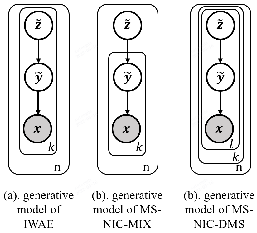
Figure 2: The generative model of Fig. 1 (d)-(f). The generative models show how we compute data likelihood for multiple-sample approaches, not how the image is actually generated in nature. For clarity, we omit the parameters.

Fig. 2 shows the generative models of Fig. 1 (d)-(f). Note that we have only one unique sample of $\bm{x}$ inside the $n$ plate, but it is repeated $k$ times for IWAE, MS-NIC-MIX and $k\times l$ times for MS-NIC-DMS. Similarly, k samples of $\bm{\tilde{y}}$ is repeated $l$ times and $l$ samples of $\bm{\tilde{z}}$ is repeated $k$ times for MS-NIC-DMS.

A.3 Proof on the Properties of MS-NIC-MIX and MS-NIC-DMS

In this section, we add the $q(\bm{\tilde{z}}|\bm{\tilde{y}}),q(\bm{\tilde{y}}|\bm{x})$ back to equations for clarity of the proof. This makes the notations slightly different from Eq. 12 and Eq. 14. Note that divide by $q(\bm{\tilde{z}}|\bm{\tilde{y}}),q(\bm{\tilde{y}}|\bm{x})$ does not effect the value of equation, and add $\log q(\bm{\tilde{z}}|\bm{\tilde{y}}),\log q(\bm{\tilde{y}}|\bm{x})$ does not effect the value of equation.

For MS-NIC-MIX to be a reasonably better approach to apply over [Ballé et al., 2018], we show that $\mathcal{L}^{MIX}_{k}$ satisfies following properties:

1. $\log p(x)\geq\mathcal{L}^{MIX}_{k}$

2. $\mathcal{L}^{MIX}_{k}\geq\mathcal{L}^{MIX}_{m}$ for $k\geq m$

We can show 1. $\log p(x)\geq\mathcal{L}^{MIX}_{k}$ by applying Jensen’s inequality twice:

$$\begin{array}[]{l}\mathcal{L}_{k}^{MIX}=\mathbb{E}_{q_{\phi}(\bm{\tilde{z}}|\bm{x})}[\mathbb{E}_{q_{\phi}(\bm{\tilde{y}}_{1:k}|\bm{x})}[\log\frac{1}{k}\overset{k}{\underset{i}{\sum}}\frac{p(\bm{x}|\bm{\tilde{y}}_{i})p(\bm{\tilde{y}}_{i}|\bm{\tilde{z}})}{q(\bm{\tilde{y}}_{i}|\bm{x})}|\bm{\tilde{z}}]+\log p(\bm{\tilde{z}})-\log q(\bm{\tilde{z}}|\bm{x})]\\ \hskip 30.00005pt\leq\mathbb{E}_{q_{\phi}(\bm{\tilde{z}}|\bm{x})}[\log(\frac{1}{k}\overset{k}{\underset{i}{\sum}}\mathbb{E}_{q_{\phi}(\bm{\tilde{y}}_{1:k}|\bm{x})}[\frac{p(\bm{x}|\bm{\tilde{y}}_{i})p(\bm{\tilde{y}}_{i}|\bm{\tilde{z}})}{q(\bm{\tilde{y}}_{i}|\bm{x})}|\bm{\tilde{z}}])+\log p(\bm{\tilde{z}})-\log q(\bm{\tilde{z}}|\bm{x})]\\ \hskip 30.00005pt=\mathbb{E}_{q_{\phi}(\bm{\tilde{z}}|\bm{x})}[\log p(\bm{x}|\bm{\tilde{z}})+\log p(\bm{\tilde{z}})-\log q(\bm{\tilde{z}}|\bm{x})]\\ \hskip 30.00005pt\leq\log(\mathbb{E}_{q_{\phi}(\bm{\tilde{z}}|\bm{x})}[\frac{p(\bm{x}|\bm{\tilde{z}})p(\bm{\tilde{z}})}{q(\bm{\tilde{z}}|\bm{x})}])\\ \hskip 30.00005pt=\log p(x)\end{array}$$ (18)

We can show 2. $\mathcal{L}^{MIX}_{k}\geq\mathcal{L}^{MIX}_{m}$ for $k\geq m$ by borrowing the Theorem 1 from IWAE paper:

$$\begin{array}[]{l}k\geq m\Rightarrow\mathbb{E}_{q(\bm{h}_{i}|\bm{x})}[\log\frac{1}{k}\overset{k}{\underset{i}{\sum}}\frac{p(\bm{h}_{i}|\bm{x})p(\bm{h}_{i})}{q(\bm{h}_{i}|\bm{x})}]\geq\mathbb{E}_{q(\bm{h}_{i}|\bm{x})}[\log\frac{1}{m}\overset{m}{\underset{i}{\sum}}\frac{p(\bm{h}_{i}|\bm{x})p(\bm{h}_{i})}{q(\bm{h}_{i}|\bm{x})}]\end{array}$$ (19)

Applying Eq. 19 to the internal part of $\mathcal{L}^{MIX}_{k}$, when $k\geq m$, we have:

$$\begin{array}[]{l}\mathcal{L}_{k}^{MIX}=\mathbb{E}_{q_{\phi}(\bm{\tilde{z}}|\bm{x})}[\mathbb{E}_{q_{\phi}(\bm{\tilde{y}}_{1:k}|\bm{x})}[\log\frac{1}{k}\overset{k}{\underset{i}{\sum}}\frac{p(\bm{x}|\bm{\tilde{y}}_{i})p(\bm{\tilde{y}}_{i}|\bm{\tilde{z}})}{q(\bm{\tilde{y}}_{i}|\bm{x})}|\bm{\tilde{z}}]+\log p(\bm{\tilde{z}})-\log q(\bm{\tilde{z}}|\bm{x})]\\ \hskip 30.00005pt\geq\mathbb{E}_{q_{\phi}(\bm{\tilde{z}}|\bm{x})}[\mathbb{E}_{q_{\phi}(\bm{\tilde{y}}_{1:m}|\bm{x})}[\log\frac{1}{m}\overset{m}{\underset{i}{\sum}}\frac{p(\bm{x}|\bm{\tilde{y}}_{i})p(\bm{\tilde{y}}_{i}|\bm{\tilde{z}})}{q(\bm{\tilde{y}}_{i}|\bm{x})}|\bm{\tilde{z}}]+\log p(\bm{\tilde{z}})-\log q(\bm{\tilde{z}}|\bm{x})]\\ \hskip 30.00005pt=\mathcal{L}^{MIX}_{m}\par\end{array}$$ (20)

For MS-NIC-DMS to be a reasonably better approach to apply over [Ballé et al., 2018] and MS-NIC-MIX, we show that $\mathcal{L}^{DMS}_{k,l}$ statisfies following properties:

1. $\log p(x)\geq\mathcal{L}^{DMS}_{k,l}$

2. $\mathcal{L}^{DMS}_{k,l}\geq\mathcal{L}^{DMS}_{m,n}$ for $k\geq m,l\geq n$

3. $\mathcal{L}^{DMS}_{k,l}\geq\mathcal{L}^{MIX}_{k}$

4. $\mathcal{L}^{DMS}_{k,l}\rightarrow\log p(x)$ as $k,l\rightarrow\infty$, under the assumption that $\log\frac{p(\bm{x}|\bm{\tilde{y}}_{i})p(\bm{\tilde{y}}_{i}|\bm{\tilde{z}}_{j})}{q(\bm{\tilde{y}}_{i}|\bm{x})}$ and $\log\frac{p(\bm{x}|\bm{\tilde{z}}_{j})p(\bm{\tilde{z}}_{j})}{q(\bm{\tilde{z}}_{j}|\bm{x})}$ are bounded.

Similar to MS-NIC-DMS, we can show 1.$\log p(x)\geq\mathcal{L}^{DMS}_{k,l}$ by applying Jensen’s inequality twice:

$$\begin{array}[]{l}\mathcal{L}_{k,l}^{DMS}=\mathbb{E}_{q_{\phi}(\bm{\tilde{z}}_{1:l}|\bm{x})}[\log\frac{1}{l}\overset{l}{\underset{j}{\sum}}\exp{(\mathbb{E}_{q_{\phi}(\bm{\tilde{y}}_{1:k}|\bm{x})}[\log\frac{1}{k}\overset{k}{\underset{i}{\sum}}\frac{p(\bm{x}|\bm{\tilde{y}}_{i})p(\bm{\tilde{y}}_{i}|\bm{\tilde{z}}_{j})}{q(\bm{\tilde{y}}_{i}|\bm{x})}|\bm{\tilde{z}}_{j}])}p(\bm{\tilde{z}}_{j})/q(\bm{\tilde{z}}_{j}|\bm{x})]\\ \hskip 30.00005pt\leq\mathbb{E}_{q_{\phi}(\bm{\tilde{z}}_{1:l}|\bm{x})}[\log\frac{1}{l}\overset{l}{\underset{j}{\sum}}\exp{\log(\frac{1}{k}\overset{k}{\underset{i}{\sum}}\mathbb{E}_{q_{\phi}(\bm{\tilde{y}}_{1:k}|\bm{x})}[p(\bm{x}|\bm{\tilde{y}}_{i})p(\bm{\tilde{y}}_{i}|\bm{\tilde{z}}_{j})|\bm{\tilde{z}}_{j}])}p(\bm{\tilde{z}}_{j})/q(\bm{\tilde{z}}_{j}|\bm{x})]\\ \hskip 30.00005pt=\mathbb{E}_{q_{\phi}(\bm{\tilde{z}}_{1:l}|\bm{x})}[\log\frac{1}{l}\overset{l}{\underset{j}{\sum}}\frac{p(\bm{x}|\bm{\tilde{z}}_{j})p(\bm{\tilde{z}}_{j})}{q(\bm{\tilde{z}}_{j}|\bm{x})}]\\ \hskip 30.00005pt\leq\log\frac{1}{l}\overset{l}{\underset{j}{\sum}}\mathbb{E}_{q_{\phi}(\bm{\tilde{z}}_{1:l}|\bm{x})}[\frac{p(\bm{x}|\bm{\tilde{z}}_{j})p(\bm{\tilde{z}}_{j})}{q(\bm{\tilde{z}}_{j}|\bm{x})}]\\ \hskip 30.00005pt=\log p(\bm{x})\end{array}$$ (21)

Also similar to MS-NIC-MIX, we can borrow conclusion from IWAE (Eq. 19) and apply it twice to show 2. $\mathcal{L}^{DMS}_{k,l}\geq\mathcal{L}^{DMS}_{m,n}$ for $k\geq m,l\geq n$:

$$\begin{array}[]{l}\mathcal{L}_{k,l}^{DMS}=\mathbb{E}_{q_{\phi}(\bm{\tilde{z}}_{1:l}|\bm{x})}[\log\frac{1}{l}\overset{l}{\underset{j}{\sum}}\exp{(\mathbb{E}_{q_{\phi}(\bm{\tilde{y}}_{1:k}|\bm{x})}[\log\frac{1}{k}\overset{k}{\underset{i}{\sum}}\frac{p(\bm{x}|\bm{\tilde{y}}_{i})p(\bm{\tilde{y}}_{i}|\bm{\tilde{z}}_{j})}{q(\bm{\tilde{y}}_{i}|\bm{x})}|\bm{\tilde{z}}_{j}])}p(\bm{\tilde{z}}_{j})/q(\bm{\tilde{z}}_{j}|\bm{x})]\\ \hskip 30.00005pt\geq\mathbb{E}_{q_{\phi}(\bm{\tilde{z}}_{1:l}|\bm{x})}[\log\frac{1}{l}\overset{l}{\underset{j}{\sum}}\exp{(\mathbb{E}_{q_{\phi}(\bm{\tilde{y}}_{1:m}|\bm{x})}[\log\frac{1}{m}\overset{m}{\underset{i}{\sum}}\frac{p(\bm{x}|\bm{\tilde{y}}_{i})p(\bm{\tilde{y}}_{i}|\bm{\tilde{z}}_{j})}{q(\bm{\tilde{y}}_{i}|\bm{x})}|\bm{\tilde{z}}_{j}])}p(\bm{\tilde{z}}_{j})/q(\bm{\tilde{z}}_{j}|\bm{x})]\\ \hskip 30.00005pt\geq\mathbb{E}_{q_{\phi}(\bm{\tilde{z}}_{1:n}|\bm{x})}[\log\frac{1}{n}\overset{n}{\underset{j}{\sum}}\exp{(\mathbb{E}_{q_{\phi}(\bm{\tilde{y}}_{1:m}|\bm{x})}[\log\frac{1}{m}\overset{m}{\underset{i}{\sum}}\frac{p(\bm{x}|\bm{\tilde{y}}_{i})p(\bm{\tilde{y}}_{i}|\bm{\tilde{z}}_{j})}{q(\bm{\tilde{y}}_{i}|\bm{x})}|\bm{\tilde{z}}_{j}])}p(\bm{\tilde{z}}_{j})/q(\bm{\tilde{z}}_{j}|\bm{x})]\\ \hskip 30.00005pt=\mathcal{L}^{DMS}_{m,n}\end{array}$$ (22)

With 2. $\mathcal{L}^{DMS}_{k,l}\geq\mathcal{L}^{DMS}_{m,n}$ for $k\geq m,l\geq n$ holds, we can show 3. $\mathcal{L}^{DMS}_{k,l}\geq\mathcal{L}^{MIX}_{k}$ immediately as $\mathcal{L}^{DMS}_{k,l}\geq\mathcal{L}^{DMS}_{k,1}=\mathcal{L}^{MIX}_{k}$.

To show 4. $\mathcal{L}^{DMS}_{k,l}\rightarrow\log p(x)$ as $k,l\rightarrow\infty$, we first define intermediate variables $W_{k},\tilde{M}_{k,l},M_{k,l}$:

$$\begin{array}[]{l}\hskip 5.0ptW_{k}=\frac{1}{k}\overset{k}{\underset{i}{\sum}}\frac{p(\bm{x}|\bm{\tilde{y}}_{i})p(\bm{\tilde{y}}_{i}|\bm{\tilde{z}}_{j})}{q(\bm{\tilde{y}}_{i}|\bm{x})}\\ \tilde{M}_{k,l}=\frac{1}{l}\overset{l}{\underset{j}{\sum}}\frac{p(\bm{x}|\bm{\tilde{z}}_{j})p(\bm{\tilde{z}}_{j})}{q(\bm{\tilde{z}}_{j}|\bm{x})}\\ M_{k,l}=\frac{1}{l}\overset{l}{\underset{j}{\sum}}\exp{(\mathbb{E}_{q_{\phi}(\bm{\tilde{y}}_{1:k}|\bm{x})}[\log W_{k}|\bm{\tilde{z}}_{j}])}p(\bm{\tilde{z}}_{j})/q(\bm{\tilde{z}}_{j}|\bm{x})\end{array}$$ (23)

Under the assumption that $\log p(\bm{x}|\bm{\tilde{y}}_{i})p(\bm{\tilde{y}}_{i}|\bm{\tilde{z}}_{j})/q(\bm{\tilde{y}}_{i}|\bm{x})$ is bounded, from the strong law of large number, we have $W_{k}\xrightarrow{a.s.}p(\bm{x}|\bm{\tilde{z}}_{j})$ (Eq. 24). Then we have $\mathbb{E}[\log W_{k}|\bm{\tilde{z}}_{j}]\rightarrow\log p(\bm{x}|\bm{\tilde{z}}_{j})$.

$$\begin{array}[]{l}W_{k}\xrightarrow{a.s.}\mathbb{E}_{q(\bm{\tilde{y}}_{i}|\bm{x})}[\frac{p(\bm{x}|\bm{\tilde{y}}_{i})p(\bm{\tilde{y}}_{i}|\bm{\tilde{z}}_{j})}{q(\bm{\tilde{y}}_{i}|\bm{x})}|\bm{\tilde{z}}_{j}]=\int q(\bm{\tilde{y}}_{i}|\bm{x})\frac{p(\bm{x}|\bm{\tilde{y}}_{i})p(\bm{\tilde{y}}_{i}|\bm{\tilde{z}}_{j})}{q(\bm{\tilde{y}}_{i}|\bm{x})}d\bm{\tilde{y}}_{i}=p(\bm{x}|\bm{\tilde{z}}_{j})\end{array}$$ (24)

Moreover, as $\mathbb{E}[\log W_{k}|\bm{\tilde{z}}_{j}]\rightarrow\log p(\bm{x}|\bm{\tilde{z}}_{j})$, we have $M_{k,l}\rightarrow\tilde{M}_{k,l}$. This means that $\forall\epsilon>0,\exists k,l,s.t.|M_{k,l}-\tilde{M}_{k,l}|<\epsilon$. And thus we have $|\mathbb{E}[M_{k,l}]-\mathbb{E}[\tilde{M}_{k,l}]|\leq\mathbb{E}[|M_{k,l}-\tilde{M}_{k,l}|]<\epsilon\rightarrow 0$. Then we have $|E[M_{k,l}]-p(\bm{x})|\leq|E[M_{k,l}]-E[\tilde{M}_{k,l}]|+|E[\tilde{M}_{k,l}]-p(\bm{x})|\rightarrow 0$, and thus $E[M_{k,l}]\rightarrow p(\bm{x})$. Finally we have $\mathbb{E}[\log M_{k,l}]=L^{DMS}_{k,l}\rightarrow\log p(\bm{x})$.

A.4 Effects of Sample Size

When comparing the R-D performance of models trained with a single $\lambda$, we use R-D cost as our metric. The R-D cost is simply computed as bpp $+\lambda$ MSE, where bpp is a short of bits-per-pixel, and MSE is a short of mean square error. The lower the R-D cost is, the better the R-D performance is. Another way to interpret R-D cost is to view it as the ELBO with constant offset. Then the $\lambda$ MSE is connected to the log likelihood of a Gaussian distribution whose mean is the output of decoder and sigma is determined by $\lambda$. Note that R-D cost is only comparable when $\lambda$ is the same.

Tab. 7 shows the effect of sample size to MS-NIC. Moreover, we compare the naïve increase of batch size versus multiple importance weighted samples. As shown by the table, increasing the batch size $\times 3-16$ only slightly affects the R-D cost (from $1.017$ to $1.013$). However, the MS-NIC-MIX can achieve R-D cost of $0.9988$ with sample size 8, and MS-NIC-DMS can achieve $0.9954$ with sample size 16. This means that MS-NIC is effective over the baseline and vanilla batch size increases. It is also noteworthy that we have not observed inference model training failure as sample size increase. While MS-NIC also suffers from gradient SNR vanishing problem, a sample size of $16$ is probably not large enough to make it evident. Limited by computational power, we can not raise sample size by several magnitudes as [Rainforth et al., 2018] does with small model.

Table 7: Effect of sample size in MS-NIC.

	Sample/Batch Size	bpp	MSE	PSNR (db)	R-D cost
Baseline [Ballé et al., 2018]	-	0.5273	32.61	33.28	1.017
Baseline-BigBatch	$\times$3	0.5308	32.51	33.31	1.018
	$\times$5	0.5285	32.51	33.30	1.016
	$\times$8	0.5279	32.37	33.34	1.013
	$\times$16	0.5321	32.12	33.38	1.014
IWAE [Burda et al., 2016]	3	0.9128	32.46	33.28	1.400
	5	0.7903	31.73	33.40	1.266
	8	0.9477	31.48	33.44	1.420
	16	1.273	31.69	33.40	1.748
MS-NIC-MIX	3	0.5238	31.80	33.40	1.000
	5	0.5259	31.84	33.38	1.003
	8	0.5260	31.52	33.44	0.9988
	16	0.5256	32.48	33.29	1.013
MS-NIC-DMS	3, 3	0.5247	32.39	33.30	1.010
	5, 5	0.5230	31.84	33.39	1.001
	8, 8	0.5255	31.55	33.43	0.9989
	16, 16	0.5249	31.38	33.46	0.9954

A.5 Detailed Experimental Settings

All the experiments are conducted on a computer with Intel(R) Xeon(R) CPU E5-2620 v4 @ 2.10GHz and $8\times$ Nvidia(R) TitanXp. All the training scripts are implemented with Pytorch 1.7 and CUDA 9.0. For experiments with single-sample, we adopt Adam optimizer with $\beta_{1}=0.90,\beta_{2}=0.95,lr=1e^{-4}$. For experiments with multiple-sample/big batch, we scale $lr$ linearly with sample size. All the models are trained for $2000$ epochs with the settings in Sec. 5.1. For first $200$ epochs, we adopt cosine annealing [Loshchilov and Hutter, 2016] to schedule learning rate. It takes around $1-2$ days to train models based on Ballé et al. [2018], and $3-5$ days to train models on Cheng et al. [2020]. Note that our multiple-sample approaches’ training time does not scale linearly with sample size, as we perform sampling on posterior, and the variational encoder only computes parameter of posterior parameters once. Further, we provide the pytorch style sudo code for implementation guidance of MS-NIC-MIX and MS-NIC-DMS.

⬇

import torch

from torch.nn import functional as F

def IWAELoss(minus_elbo):

”’

args

—-

minus_elbo: tensor, [b, k], which is R + \lambda D

return

——

local iwae loss

”’

# this is the minus ELBO related to y part,

# to get the real ELBO:

log_weights = - minus_elbo.detach()

# no gradient given to weights

weights = F.softmax(log_weights, dim=1) # B, K

loss_b = torch.sum(minus_elbo * weights, dim=1, keepdim=False)

loss_iwae = torch.mean(loss_b)

return loss_iwae

def DMSLoss(x, x_hat, y_likelihood, z_likelihood, lam):

”’

args

—-

x: original image: [b, c, h, w]

x_hat: reconstructed image: [b, k, c, h, w], k is the

number of samples

y_likelihood: [b, 192/320, h//8, w//8, k^2],

as original paper of [Balle et al. 2018], the number of

channels 192/320 is determined by lambda, k^2 is the

number of samples in DMS setting, with MS-NIC-MIX,

this k^2 is k

z_likelihood: [b, 128/192, h//64, w//64, k], as original

paper of [Balle et al. 2018], the number of channels

128/192 is determined by lambda,

k is the number of samples

return

——

total iwae loss

”’

b, c, h, w = x.shape

k = x_hat.shape[0] // x.shape[0]

x = torch.repeat_interleave(x, repeats=k, dim=0)

x = x.reshape(b, k, c, h, w)

x_hat = x_hat.reshape(b, k, c, h, w)

d_loss = torch.mean(lam * 65025 * (x - x_hat)**2, dim=(2,3,4),

keepdim=False)

yz_loss = -torch.sum(torch.log2(y_likelihood), dim=(1,2,3)).\

reshape(b, -1) / (h * w)

z_loss = -torch.sum(torch.log2(z_likelihood), dim=(1,2,3)).\

reshape(b, -1) / (h * w)

local_d = IWAELoss(d_loss)

local_yz = IWAELoss(yz_loss)

local_z = IWAELoss(z_loss)

loss_total = local_d + local_yz + local_z

return loss_total

A.6 Detailed Experimental Results

In this section we present more detailed experimental results in Tab. 8 and Tab. 5. Note that without direct-y trick, the IWAE for Cheng et al. [2020] totally fails and we can not produce a valid BD metric from it.

Table 8: Detailed results based on [Ballé et al., 2018].

	$\lambda$	bpp	MSE	PSNR (db)	MS-SSIM
Baseline [Ballé et al., 2018]	0.0016	0.1205	138.4	27.23	0.9111
	0.0032	0.1990	91.52	28.95	0.9384
	0.0075	0.3492	52.68	31.28	0.9624
	0.015	0.5270	32.78	33.28	0.9766
	0.03	0.7626	19.90	35.37	0.9847
	0.045	0.9249	15.69	36.39	0.9883
	0.08	1.211	10.04	38.27	0.9919
IWAE [Burda et al., 2016]	0.0016	0.2559	144.7	27.12	0.9134
	0.0032	0.3478	90.65	29.03	0.9389
	0.0075	0.5931	51.40	31.38	0.9642
	0.015	0.7902	31.73	33.40	0.9765
	0.03	1.135	19.41	35.47	0.9850
	0.045	1.886	14.70	36.65	0.9885
	0.08	1.753	9.898	38.32	0.9919
MS-NIC-MIX	0.0016	0.1132	146.4	27.08	0.9121
	0.0032	0.1967	88.44	29.15	0.9409
	0.0075	0.3496	51.27	31.39	0.9632
	0.015	0.5260	31.52	33.43	0.9773
	0.03	0.7591	19.33	35.49	0.9851
	0.045	0.9248	14.43	36.72	0.9885
	0.08	1.201	9.694	38.40	0.9919
MS-NIC-DMS	0.0016	0.1173	135.1	27.38	0.9145
	0.0032	0.1967	86.07	29.26	0.9413
	0.0075	0.3495	49.98	31.51	0.9647
	0.015	0.5250	31.36	33.46	0.9771
	0.03	0.7546	19.81	35.37	0.9846
	0.045	0.9220	14.74	36.61	0.9883
	0.08	1.196	9.637	38.43	0.9920

Table 9: Detailed results based on [Cheng et al., 2020].

	$\lambda$	bpp	MSE	PSNR (db)	MS-SSIM
Baseline [Cheng et al., 2020]	0.0016	0.1205	138.4	27.23	0.9111
	0.0032	0.1990	91.52	28.95	0.9384
	0.0075	0.3492	52.68	31.28	0.9624
	0.015	0.5270	32.78	33.28	0.9766
	0.03	0.6424	19.48	35.54	0.9855
	0.045	0.7846	15.48	36.53	0.9885
	0.08	1.026	11.41	37.87	0.9916
IWAE [Burda et al., 2016]	0.0016	3.226	109.1	28.32	0.9182
	0.0032	3.407	78.07	29.74	0.9414
	0.0075	3.555	47.19	31.84	0.9652
	0.015	3.445	31.84	33.56	0.9779
	0.03	3.534	23.66	34.92	0.9849
	0.045	3.545	20.63	35.59	0.9878
	0.08	3.157	16.40	36.62	0.9908
MS-NIC-MIX	0.0016	0.1068	109.7	28.30	0.9171
	0.0032	0.1636	78.07	29.71	0.9404
	0.0075	0.2861	47.29	31.85	0.9651
	0.015	0.4309	31.88	33.55	0.9777
	0.03	0.6586	19.11	35.60	0.9853
	0.045	0.8007	14.65	36.76	0.9889
	0.08	1.034	10.93	38.00	0.9916
MS-NIC-DMS	0.0016	0.1043	109.8	28.30	0.9163
	0.0032	0.1644	77.44	29.74	0.9412
	0.0075	0.2849	47.30	31.85	0.9656
	0.015	0.4306	32.22	33.51	0.9775
	0.03	0.6432	18.94	35.65	0.9856
	0.045	0.7926	14.84	36.67	0.9886
	0.08	1.039	10.48	38.18	0.9918

A.7 Distribution of Latent Variance

We show the histogram of latent variance in log space in Fig. 3. From the histogram we can observe that for latent $\bm{y}$, the variance distribution of two MS-NIC approaches is similar and single-sample approach is quite different. MS-NIC has more latent dimensions that have high variance (the right mode), and less with low variance (the left mode). Moreover, the low variance mode of MS-NIC has less variance than single-sample approach, which indicates that MS-NIC does a better job in separating active and inactive latent dimensions. Similarly, the low variance mode of $\bm{\tilde{z}}$ in MS-NIC approaches is lower than single-sample approach.

Table 10: The average of per-dimension latent variance and Cov across Kodak test images. The model is trained with $\lambda=0.015$.

	Var(#)		Cov(#)
Method	$\bm{y}$	$\bm{z}$	$\bm{y}$	$\bm{z}$
Single-sample
Ballé et al. [2018]	1.512	0.3356	20.36	14.48
Multiple-sample
MS-NIC-MIX	1.909	0.7705	114.4	7.234
MS-NIC-DMS	1.908	0.7522	93.67	7.024

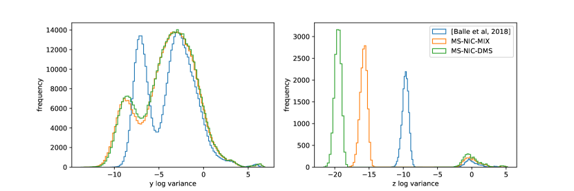
Figure 3: The histogram of log space per-dimension latent variance across Kodak test images. The model is trained with $\lambda=0.015$.

A.8 Tighter ELBO for Inference Time

A.8.1 Inference time ELBO and Softmin Coding [Theis and Ho, 2021]

The inference time tighter ELBO is another under-explored issue. In fact, the training time tighter ELBO and inference time ELBO is independent. We can train a model with tighter ELBO, infer with single sample ELBO. Or we can also conduct multiple sample infer on a model trained with single sample. The general idea is:

• The training time tighter ELBO benefits the performance in terms of avoiding posterior collapse. As we state and empirically verify in Sec. 5.3. We adopt deterministic rounding during inference time, and there is no direct connection between the training time tighter ELBO and inference time R-D cost. However, we indeed end up with a richer latent space (Sec. 5.3), which means more active latent dimensions and less bitrate waste.

• The inference time tighter ELBO sounds really alluring for compression community. However, there remains two pending issue to be resolved prior to the application of the inference time tighter ELBO: 1) How this inference time multiple-sample ELBO is related to R-D cost remains under-explored. In other words, whether the entropy coding itself can achieve the R-D cost defined by multiple-sample ELBO is a question. 2) The inference time multiple-sample ELBO only makes sense with stochastic encoder (you can not importance weight the same deterministic ELBO), whose impact on lossy compression remains dubious.

For the first pending issue, the softmin coding [Theis and Ho, 2021] is proposed to achieve multiple sample ELBO based on Universal Quantization (UQ) [Agustsson and Theis, 2020]. However, it is not a general method and is tied to UQ. Moreover, as we stated in Sec 4.3, its computational cost is forbiddingly high and its improvement is marginal. But those are not the real problem of softmin coding. Instead, the real problem is the second pending issue: stochastic lossy encoder. The softmin coding relies on UQ, and UQ relies on stochastic lossy encoder. And the stochastic lossy encoder is exactly the second issue that we want to discuss.

A.8.2 Stochastic Lossy Encoder and Universal Quantization

It is known to lossless compression community that stochastic lossy encoder benefits compression performance [Ryder et al., 2022] with the aid of bits-back coding [Townsend et al., 2018]. While the bits-back coding is not applicable to lossy compression. For lossy compression, currently we know that the stochastic encoder degrades R-D performance especially when distortion is measured in MSE [Theis and Agustsson, 2021]. In the original UQ paper, the performance decay of vanilla UQ over deterministic rounding is obvious ($\approx 1$db). When we writing this paper, we also find the performance decay of UQ is quite high. As shown in Tab. 11, the R-D cost of UQ is significantly higher than deterministic rounding. This negative result makes softmin coding less promising than it seems as it only obtains a marginal gain over UQ.

	y bpp	z bpp	MSE	RD Cost
Deterministic Rounding	0.3347	0.01418	26.86	0.7552
Universal Quantization	0.5379	0.01431	23.94	0.9080

Table 11: The R-D performance of UQ vs deterministic rounding on the first image of Kodak dataset.

In our humble opinion, this performance decay of UQ is partially brought by stochastic encoder itself. For lossless compression, the deterministic encoder and stochastic encoder are just two types of bit allocation preference:

• The deterministic encoder allocate less bitrate to $\log p(y)$, more to $\log p(x|y)$ and $0$ to $\log q(y|x)$.

• The stochastic encoder allocate more bitrate to $\log p(y)$, less to $\log p(x|y)$ and minus bitrate to $\log q(y|x)$

Therefore, for lossless compression, it is reasonable that the bitrate increase to $\log p(y)$ and $\log p(x|y)$ can be offset by bits-back coding bitrate $\log q(y|x)$. While for lossy compression, there is no way to bits-back $\log q(y|x)$ (as we can not reconstruct $q(y|x)$ without $x$). If the bitrate increase in $\log p(y)$ and $\log p(x|y)$, the R-D cost just increases for lossy compression. Prior to other entropy coding bitrate that is able to achieve R-D cost equals to minus ELBO with $E_{q}[\log q]\neq 0$ becomes mature (such as relative entropy coding [Flamich et al., 2020]), we have no way to implement a stochastic lossy encoder with reasonable R-D performance. By now, we have no good way to achieve tighter ELBO during inference time.

A.8.3 Training-Testing Distribution Mismatch and Universal Quantization

Moreover, whether the quantization error is uniform distribution remains a question. And we think that is another reason why UQ does not work well. In fact, the real distribution of quantization noise is pretty much a highly concentrated distribution around $0$ (See Fig. 4). And it is quite far away from uniform distribution, which violates the assumption of Ballé et al. [2018]. We also find that this concentrated distribution is caused by that most of latent dimension is quite close to $0$. The evidence is, if we remove the latent dimension $y^{i}\in[-0.5,0.5]$, then the quantization noise looks similar to a uniform distribution (See Fig. 4). So, if we apply direct rounding, they are kept as $0$ and the latent is sparse. However, adding uniform noise to it loses this sparsity, which result in bitrate increase. And from Tab. 11, we can wee that the UQ reduce MSE while increase the bitrate. From total R-D cost perspective, the deterministic rounding outperforms UQ. As a matter of fact, the assumption of UQ that resolving training-testing distribution mismatch improves R-D performance does not hold well. To wrap up, we find that there is some pending issues to be resolved prior to the practical solution of tighter ELBO for inference time.

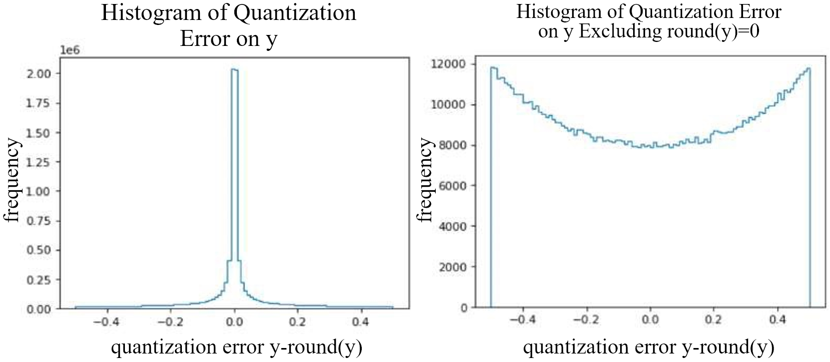
Figure 4: The histogram of $\bm{y}-\bar{\bm{y}}$ of first image of Kodak dataset.

A.9 The Effect on Training Time

The MS-NIC-MIX and MS-NIC-DMS is more time efficient than simply increase batchsize. For MS-NIC-MIX with $k$ samples, the $y$ encoder $q(y|x)$ is inferred with only 1 sample, and the $z$ encoder, decoder and entropy model $q(z|x),p(y|z),p(z)$ is inferred with only 1 sample. And only the $y$ decoder $p(x|y)$ is inferred $k$ times. This sample efficiency makes the training time grows slowly with $k$. In our experiment, the MS-NIC-MIX with 8 samples only increases the training time by $\times 1.5$, the MS-NIC-MIX with $16$ samples only increases the training time by $\times 3$. The MS-NIC-DMS is slightly slower, as the $z$ entropy model and decoder $p(z),p(y|z)$ also requires $k$ times inference. However, it is still much more efficient than batchsize $\times k$ as all the encoders $q(y|x),q(z|x)$ requires only 1 inference. In fact, sampling from posterior is much cheaper than inferring the posterior parameters. Similar spirit has also been adopted in improving the efficiency of sampling from Gumbel-Softmax relaxed posterior [Paulus et al., 2020].

The trade-off between batchsize and sample number is a more subtle issue. As stated in Rainforth et al. [2018], the gradient SNR of encoder (inference model) scales with $\Theta(M/K)$, and the gradient SNR of decoder (generative model) scales with $\Theta(M/K)$, where M is the batchsize and K is the sample size. Another assumption required prior to further discussion is that the suboptimality of VAE mainly comes from inference model [Cremer et al., 2018], which means that the encoder is harder to train than the decoder. This means that an infinitely large $K$ ruins the convergence of encoder, and solemnly increasing sample number frustrates training. In practice the overall performance is determined by both inference suboptimality and ELBO-likelihood gap. In a word, we believe there is no general answer for all problem. But a reasonable balance between sample size and batchsize is the golden rule to maximize performance (as $T(M)$ and $T(K)$ grow linearly with batchsize/sample size). And the obvious case is that neither setting batchsize to $M=1$ and give all resources to $K$, nor setting sample size $K=1$ and give all resources to $M$ is optimal.

A.10 More Limitation and Discussion

The cause of negative results on MS-SSIM of Cheng et al. [2020] is more complicated. One possible explanation is that the gradient property of Cheng et al. [2020] is not as good as Ballé et al. [2018]. As a reference, the training of [Burda et al., 2016] totally fails on Cheng et al. [2020] and produces garbage R-D results (See Tab. 9). This bad gradient property might account for the bad results of MS-SSIM on Cheng et al. [2020], as the gradient of IWAE and MS-NIC is certainly trickier than the gradient of single sample approaches.

As evidence, when we are studying the stability of the network in Cheng et al. [2020], we find that without limitation of entropy model (imagine setting $\lambda$ to $\infty$) and quantization, Cheng et al. [2020] produces PSNR of $43.27$db, while Ballé et al. [2018] produces PSNR of $48.54$db. This means that Cheng et al. [2020] is not as good as Ballé et al. [2018] as an auto-encoder. Moreover, when we finetune these pre-trained model into a lossy compression model, Cheng et al. [2020] produces $nan$ results while Ballé et al. [2018] converges. This result indicates that the backbone of Cheng et al. [2020]’s gradient is probably more difficult to deal with than Ballé et al. [2018].

A.11 Broader Impact

Improving the R-D performance of NIC methods is valuable itself. It is beneficial to reducing the carbon emission by reducing the resources required to transfer and store images. And NIC has potential of saving network channel bandwidth and disk storage over traditional codecs. Moreover, for traditional codecs, usually dedicated hardware accelerators are required for efficient decoding. This codec-hardware bondage hinders the wide adaptation of new codecs. Despite the sub-optimal R-D performance of old codecs such as JPEG, H264, they are still prevalent due to broad hardware support. While modern codecs such as H266 [Bross et al., 2021] can not be widely adopted due to limited hardware decoder deployment. However, for NIC, the general purpose neural processors are able to fit to all codecs. Thus the neural decoders have better hardware flexibility, and the cost to update neural decoder only involves software, which encourages the adoption of newer methods with better R-D performance.

References

- Agustsson and Theis [2020] E. Agustsson and L. Theis. Universally quantized neural compression. Advances in neural information processing systems, 33:12367–12376, 2020.
- Agustsson et al. [2020] E. Agustsson, D. Minnen, N. Johnston, J. Balle, S. J. Hwang, and G. Toderici. Scale-space flow for end-to-end optimized video compression. In Proceedings of the IEEE/CVF Conference on Computer Vision and Pattern Recognition, pages 8503–8512, 2020.
- Ballé et al. [2017] J. Ballé, V. Laparra, and E. P. Simoncelli. End-to-end optimized image compression. In International Conference on Learning Representations, 2017.
- Ballé et al. [2018] J. Ballé, D. Minnen, S. Singh, S. J. Hwang, and N. Johnston. Variational image compression with a scale hyperprior. In International Conference on Learning Representations, 2018.
- Bauer and Mnih [2021] M. Bauer and A. Mnih. Generalized doubly reparameterized gradient estimators. In International Conference on Machine Learning, pages 738–747. PMLR, 2021.
- Bjontegaard [2001] G. Bjontegaard. Calculation of average psnr differences between rd-curves. VCEG-M33, 2001.
- Bross et al. [2021] B. Bross, J. Chen, J.-R. Ohm, G. J. Sullivan, and Y.-K. Wang. Developments in international video coding standardization after avc, with an overview of versatile video coding (vvc). Proceedings of the IEEE, 109(9):1463–1493, 2021.
- Burda et al. [2016] Y. Burda, R. B. Grosse, and R. Salakhutdinov. Importance weighted autoencoders. In ICLR (Poster), 2016.
- Chen et al. [2017] X. Chen, D. P. Kingma, T. Salimans, Y. Duan, P. Dhariwal, J. Schulman, I. Sutskever, and P. Abbeel. Variational lossy autoencoder. In International Conference on Learning Representations, 2017.
- Cheng et al. [2020] Z. Cheng, H. Sun, M. Takeuchi, and J. Katto. Learned image compression with discretized gaussian mixture likelihoods and attention modules. In Proceedings of the IEEE/CVF Conference on Computer Vision and Pattern Recognition, pages 7939–7948, 2020.
- Choi et al. [2018] K. Choi, K. Tatwawadi, T. Weissman, and S. Ermon. Necst: neural joint source-channel coding. 2018.
- Cremer et al. [2017] C. Cremer, Q. Morris, and D. Duvenaud. Reinterpreting importance-weighted autoencoders. 2017.
- Cremer et al. [2018] C. Cremer, X. Li, and D. Duvenaud. Inference suboptimality in variational autoencoders. In International Conference on Machine Learning, pages 1078–1086. PMLR, 2018.
- Dayan et al. [1995] P. Dayan, G. E. Hinton, R. M. Neal, and R. S. Zemel. The helmholtz machine. Neural computation, 7(5):889–904, 1995.
- Deng et al. [2009] J. Deng, W. Dong, R. Socher, L.-J. Li, K. Li, and L. Fei-Fei. Imagenet: A large-scale hierarchical image database. In 2009 IEEE conference on computer vision and pattern recognition, pages 248–255. Ieee, 2009.
- Flamich et al. [2020] G. Flamich, M. Havasi, and J. M. Hernández-Lobato. Compressing images by encoding their latent representations with relative entropy coding. Advances in Neural Information Processing Systems, 33:16131–16141, 2020.
- Gao et al. [2021] G. Gao, P. You, R. Pan, S. Han, Y. Zhang, Y. Dai, and H. Lee. Neural image compression via attentional multi-scale back projection and frequency decomposition. In Proceedings of the IEEE/CVF International Conference on Computer Vision, pages 14677–14686, 2021.
- Guo et al. [2021a] Z. Guo, Z. Zhang, R. Feng, and Z. Chen. Causal contextual prediction for learned image compression. IEEE Transactions on Circuits and Systems for Video Technology, 2021a.
- Guo et al. [2021b] Z. Guo, Z. Zhang, R. Feng, and Z. Chen. Soft then hard: Rethinking the quantization in neural image compression. In International Conference on Machine Learning, pages 3920–3929. PMLR, 2021b.
- He et al. [2021] D. He, Y. Zheng, B. Sun, Y. Wang, and H. Qin. Checkerboard context model for efficient learned image compression. In Proceedings of the IEEE/CVF Conference on Computer Vision and Pattern Recognition, pages 14771–14780, 2021.
- He et al. [2022] D. He, Z. Yang, W. Peng, R. Ma, H. Qin, and Y. Wang. Elic: Efficient learned image compression with unevenly grouped space-channel contextual adaptive coding. arXiv preprint arXiv:2203.10886, 2022.
- Hinton and Van Camp [1993] G. E. Hinton and D. Van Camp. Keeping the neural networks simple by minimizing the description length of the weights. In Proceedings of the sixth annual conference on Computational learning theory, pages 5–13, 1993.
- Hinton et al. [1995] G. E. Hinton, P. Dayan, B. J. Frey, and R. M. Neal. The" wake-sleep" algorithm for unsupervised neural networks. Science, 268(5214):1158–1161, 1995.
- Hu et al. [2021] Z. Hu, G. Lu, and D. Xu. Fvc: A new framework towards deep video compression in feature space. In Proceedings of the IEEE/CVF Conference on Computer Vision and Pattern Recognition, pages 1502–1511, 2021.
- Kingma and Welling [2013] D. P. Kingma and M. Welling. Auto-encoding variational bayes. arXiv preprint arXiv:1312.6114, 2013.
- Kodak [1993] E. Kodak. Kodak lossless true color image suite. http://r0k.us/graphics/kodak/, 1993.
- Li et al. [2021] J. Li, B. Li, and Y. Lu. Deep contextual video compression. Advances in Neural Information Processing Systems, 34, 2021.
- Loshchilov and Hutter [2016] I. Loshchilov and F. Hutter. Sgdr: Stochastic gradient descent with warm restarts. arXiv preprint arXiv:1608.03983, 2016.
- Lu et al. [2019] G. Lu, W. Ouyang, D. Xu, X. Zhang, C. Cai, and Z. Gao. Dvc: An end-to-end deep video compression framework. In Proceedings of the IEEE/CVF Conference on Computer Vision and Pattern Recognition, pages 11006–11015, 2019.
- Lu et al. [2020] G. Lu, X. Zhang, W. Ouyang, L. Chen, Z. Gao, and D. Xu. An end-to-end learning framework for video compression. IEEE transactions on pattern analysis and machine intelligence, 43(10):3292–3308, 2020.
- Minnen and Singh [2020] D. Minnen and S. Singh. Channel-wise autoregressive entropy models for learned image compression. In 2020 IEEE International Conference on Image Processing (ICIP), pages 3339–3343. IEEE, 2020.
- Minnen et al. [2018] D. Minnen, J. Ballé, and G. D. Toderici. Joint autoregressive and hierarchical priors for learned image compression. Advances in neural information processing systems, 31, 2018.
- Mnih and Gregor [2014] A. Mnih and K. Gregor. Neural variational inference and learning in belief networks. In International Conference on Machine Learning, pages 1791–1799. PMLR, 2014.
- Mnih and Rezende [2016] A. Mnih and D. Rezende. Variational inference for monte carlo objectives. In International Conference on Machine Learning, pages 2188–2196. PMLR, 2016.
- Mohamed et al. [2020] S. Mohamed, M. Rosca, M. Figurnov, and A. Mnih. Monte carlo gradient estimation in machine learning. J. Mach. Learn. Res., 21(132):1–62, 2020.
- Nowozin [2018] S. Nowozin. Debiasing evidence approximations: On importance-weighted autoencoders and jackknife variational inference. In International conference on learning representations, 2018.
- Paulus et al. [2020] M. B. Paulus, C. J. Maddison, and A. Krause. Rao-blackwellizing the straight-through gumbel-softmax gradient estimator. arXiv preprint arXiv:2010.04838, 2020.
- Rainforth et al. [2018] T. Rainforth, A. Kosiorek, T. A. Le, C. Maddison, M. Igl, F. Wood, and Y. W. Teh. Tighter variational bounds are not necessarily better. In International Conference on Machine Learning, pages 4277–4285. PMLR, 2018.
- Roeder et al. [2017] G. Roeder, Y. Wu, and D. K. Duvenaud. Sticking the landing: Simple, lower-variance gradient estimators for variational inference. Advances in Neural Information Processing Systems, 30, 2017.
- Ryder et al. [2022] T. Ryder, C. Zhang, N. Kang, and S. Zhang. Split hierarchical variational compression. In Proceedings of the IEEE/CVF Conference on Computer Vision and Pattern Recognition, pages 386–395, 2022.
- Serban et al. [2017] I. Serban, A. Sordoni, R. Lowe, L. Charlin, J. Pineau, A. Courville, and Y. Bengio. A hierarchical latent variable encoder-decoder model for generating dialogues. In Proceedings of the AAAI Conference on Artificial Intelligence, volume 31, 2017.
- Song et al. [2020] Y. Song, M. Xu, L. Yu, H. Zhou, S. Shao, and Y. Yu. Infomax neural joint source-channel coding via adversarial bit flip. In Proceedings of the AAAI Conference on Artificial Intelligence, volume 34, pages 5834–5841, 2020.
- Theis and Agustsson [2021] L. Theis and E. Agustsson. On the advantages of stochastic encoders. arXiv preprint arXiv:2102.09270, 2021.
- Theis and Ho [2021] L. Theis and J. Ho. Importance weighted compression. In Neural Compression: From Information Theory to Applications–Workshop@ ICLR 2021, 2021.
- Theis et al. [2017] L. Theis, W. Shi, A. Cunningham, and F. Huszár. Lossy image compression with compressive autoencoders. arXiv preprint arXiv:1703.00395, 2017.
- Toderici et al. [2015] G. Toderici, S. M. O’Malley, S. J. Hwang, D. Vincent, D. Minnen, S. Baluja, M. Covell, and R. Sukthankar. Variable rate image compression with recurrent neural networks. arXiv preprint arXiv:1511.06085, 2015.
- Toderici et al. [2017] G. Toderici, D. Vincent, N. Johnston, S. Jin Hwang, D. Minnen, J. Shor, and M. Covell. Full resolution image compression with recurrent neural networks. In Proceedings of the IEEE conference on Computer Vision and Pattern Recognition, pages 5306–5314, 2017.
- Townsend et al. [2018] J. Townsend, T. Bird, and D. Barber. Practical lossless compression with latent variables using bits back coding. In International Conference on Learning Representations, 2018.
- Tucker et al. [2018] G. Tucker, D. Lawson, S. Gu, and C. J. Maddison. Doubly reparameterized gradient estimators for monte carlo objectives. 2018.
- Van Den Oord et al. [2017] A. Van Den Oord, O. Vinyals, et al. Neural discrete representation learning. Advances in neural information processing systems, 30, 2017.
- Williams [1992] R. J. Williams. Simple statistical gradient-following algorithms for connectionist reinforcement learning. Machine learning, 8(3):229–256, 1992.
- Xie et al. [2021] Y. Xie, K. L. Cheng, and Q. Chen. Enhanced invertible encoding for learned image compression. In Proceedings of the 29th ACM International Conference on Multimedia, pages 162–170, 2021.
- Yang et al. [2020] Y. Yang, R. Bamler, and S. Mandt. Improving inference for neural image compression. Advances in Neural Information Processing Systems, 33:573–584, 2020.
- Zhu et al. [2022] X. Zhu, J. Song, L. Gao, F. Zheng, and H. T. Shen. Unified multivariate gaussian mixture for efficient neural image compression. arXiv preprint arXiv:2203.10897, 2022.
- Zhu et al. [2021] Y. Zhu, Y. Yang, and T. Cohen. Transformer-based transform coding. In International Conference on Learning Representations, 2021.