Label Distribution Learning via Implicit Distribution Representation

Abstract

In contrast to multi-label learning, label distribution learning characterizes the polysemy of examples by a label distribution to represent richer semantics. In the learning process of label distribution, the training data is collected mainly by manual annotation or label enhancement algorithms to generate label distribution. Unfortunately, the complexity of the manual annotation task or the inaccuracy of the label enhancement algorithm leads to noise and uncertainty in the label distribution training set. To alleviate this problem, we introduce the implicit distribution in the label distribution learning framework to characterize the uncertainty of each label value. Specifically, we use deep implicit representation learning to construct a label distribution matrix with Gaussian prior constraints, where each row component corresponds to the distribution estimate of each label value, and this row component is constrained by a prior Gaussian distribution to moderate the noise and uncertainty interference of the label distribution dataset. Finally, each row component of the label distribution matrix is transformed into a standard label distribution form by using the self-attention algorithm. In addition, some approaches with regularization characteristics are conducted in the training phase to improve the performance of the model.

1 Introduction

Label distribution learning (LDL) (Geng (2016)) is a novel learning paradigm that characterizes the polysemy of examples. In LDL, the relevance of each label to an example is given by an exact numerical value between 0 and 1 (also known as description degree), and the description degree of all labels forms a distribution to fully characterize the polysemy of an example. Compared with traditional learning paradigms, LDL is a more generalizable and representational learning paradigm that provides richer semantic information.

LDL has been successful in several application domains (Gao et al. (2018); Zhao et al. (2021); Chen et al. (2021a); Si et al. (2022)). To obtain the label distribution for learning, there are mainly two ways: one is expert labeling, but labeling is expensive and there is no objective labeling criterion, and the resulting label distribution is highly subjective and ambiguous. The other is to convert a multi-label dataset into a label distribution dataset through a label enhancement algorithm (Xu et al. (2019; 2020); Zheng et al. (2021a); Zhao et al. (2022)). However, label enhancement lacks a reliable theory to ensure that the label distribution recovered from logical labels converges to the true label distribution, because logical labels provide a very loose solution space for the label distribution, making the solution less stable and less accurate.

In summary, the label distribution dataset used for training has a high probability of inaccuracy and uncertainty, which significantly limits the performance of LDL algorithms. To characterize and mitigate the uncertainty of the label distribution, we propose a novel LDL method based on the implicit label distribution representation. Our work is inspired by recent work on implicit neural representation in 2D image reconstruction (Sitzmann et al. (2020)). The key idea of implicit neural representation is to represent an object as a function that maps a sequence of coordinates to the corresponding signal, where the function is de-parameterized by a deep neural network. In this paper, we start with a deep network to extract the latent features of input information. Then, the latent features are looked up against the encoded coordinate matrix to generate a label distribution matrix (implicit distribution representation). Finally, the label distribution matrix is computed by a self-attention module to yield a standard label distribution. Note that the goal of the proposed implicit distribution representation is to generate a label distribution matrix with Gaussian distribution constraints as a customized representation pattern.

To efficiently generate latent features around the coordinate, we design a deep spiking neural network (Yamazaki et al. (2022)) with an MLP as an executor to extract latent features in the input information. The architecture of the whole network consists of multiple layers of linear spiking neurons, and the neurons of different layers conduct a shortcut between them. Notably, spiking neural networks have two key properties that are different from the representation of artificial neural networks. First, a standard spiking neural network considers the time characteristics $T$ (taking the image as an example, the input tensor $X\in$ ${\mathbb{R}}^{T\times C\times W\times H}$.) at a multi-step inference mechanism. Here, we create several pseudo-feature spaces on the native feature space by setting different strategies with data augmentation (Ucar et al. (2021)). These pseudo-features and the native feature are stacked in the time dimension $T$ to achieve the multi-step inference mechanism. Second, the representation capability of the spiking neural network is underpowered, since the output space is a binarized sequence ({0 $\cdots$ 1}). Therefore, we place a standard MLP in the last layer of the spiking neural network, which projects the features into the real number space. Our model saves about 30$\sim$40$\%$ of energy consumption over ANNs with the same network structure on embedded devices such as lynxi HP300, Raspberry Pi, or Apple smartphones (PyTorch 1.2 support M1 Mac).

[capbesideposition=right,top,capbesidewidth=5.3cm]figure[]

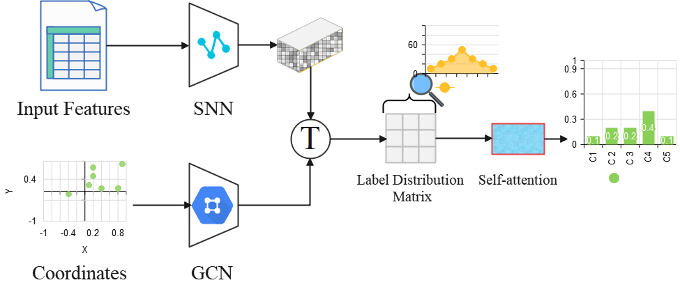
Figure 1: Our architecture. This figure shows the architecture of the proposed deep implicit function, which consists of two parts. The first part starts with a latent feature prediction stream (SNN with an MLP) that learns the input information to predict the feature maps. The second part learns a label distribution matrix to regress a label distribution.

The extraction of latent features provides material for the coordinates to generate the label distribution matrix. First, the initialized coordinate matrix (the size is $L\times 64$, where $L$ denotes the number of labels, and 64 denotes features of the nodes) is reconstructed by using a GCN. Note that the features of the nodes meet the Gaussian distribution since the deep network needs to reconstruct the data from a fixed distribution. Then the coordinate matrix is repeated in $N$ copies, and $N$ denotes the number of samples. Next, the coordinate matrix computes a label distribution matrix (the size is $N\times L\times 2L$) in the latent feature space by looking up the table. Each component of the label distribution matrix represents the distribution of each label value, and the components are constrained by a priori Gaussian distributions. Finally, the label distribution matrix leverages a self-attention mechanism to obtain the corresponding label distribution of the samples.

Yet, deep learning-based approaches are prone to overfitting manually extracted features. To alleviate the problem, we propose some regularization approaches to boost the performance of the model, and a new dataset based on the image comprehension task is released. Our contribution includes: (i) For LDL, this is a novel method to obtain the label distribution of a sample through the implicit distribution representation. (ii) Spiking neural network with an MLP is developed to save energy consumption of mobile devices, and correlations between labels are deeply mined by a graph convolutional network. (iii) Facing the LDL task, some regularization techniques are designed to boost the performance of the model and a new LDL dataset is released.

2 Proposed Method

As shown in Figure 1, our architecture is a two-stage scheme, which is based on an implicit representation approach. In the first stage (latent feature extraction), the raw features $\mathcal{X}$ are fed into the encoder for encoding to construct a latent feature space $F_{f}\in$ ${\mathbb{R}}^{L\times H\times W}$. In the second stage (label distribution matrix learning), the coordinate tensor (coordinate matrix is reshaped after GCN) $C_{r}\in$ ${\mathbb{R}}^{L\times L\times 2)}$ is looked up in the latent feature space $F_{f}$ to generate a label distribution matrix $\mathcal{M}\in$ ${\mathbb{R}}^{L\times 2L}$, and finally a label distribution $\mathcal{D}$ is obtained by using self-attention algorithm. Furthermore, some regularization terms are introduced to our model to boost its performance.

Latent Feature Extraction. Our model starts with a latent feature extraction task, which is based on a spiking neural network. Spiking neural networks have a high potential value as a 3rd deep model and are efficient and interpretable. In the LDL task, we develop a non-fixed Network Architecture and a Network Implementation due to the diversity of LDL dataset formats.

Network Architecture: Our network consists of 17 layers of function units, which include 8 linear units, 8 nonlinear units, and a transformation layer (including an MLP, a mean operator, and a reshape operator). Essentially, this is a residual network and the transformation layer at the tail of the network. Except for the first layer (the number of neurons is the dimensionality of the input features), each linear unit contains 1024 neurons, followed closely by a ReLU non-linearity, and the last layer is a reshape function to generate the feature space $F_{f}$. On datasets with a smaller feature space $\mathcal{X}$ (e.g., Gene dataset has only 36 features), each linear layer includes 64 neurons. We also attempted to use other activation functions than ReLU, such as PReLU, Swish, and Sigmoid, but without any advantage. Besides, since the spiking network involves a time dimension, the time dimension $T$ is squeezed in the output space of the spiking network by using a mean operator. The network’s tailgate should notice that the feature map is reshaped as $F_{f}$ using a reshape operator and the MLP (the number of neurons is $L\times W\times H$.), where $H$ and $W$ are 32.

Network Implementations: The simplified residual network is implemented as an ANN in two frameworks: PyTorch 1.12 (a standard deep network training library) and SpikingJelly 0.0.13 (a library for deep learning applications that is part of the PyTorch ecosystem). The SpikingJelly implementation can be run in spiking or non-spiking modes. To train the spiking network, we use an ANN-SNN conversion training approach. The conversion is simple, we convert the trained model on PyTorch with the help of an ann2snn.Converter (SpikingJelly) to obtain an SNN model. Note that the conversion method defines six modes (max, $99.9\%$, $1.0\backslash 2$, $1.0\backslash 3$, $1.0\backslash 4$, $1.0\backslash 5$) to obtain SNN with different accuracy, and in this paper, we chose $99.9\%$. The literature (Patel et al. (2021)) provides a theoretical basis for analyzing the conversion of ANN to SNN.

Label Distribution Matrix Learning. Inspired by confident learning (Northcutt et al. (2021)), we develop a matrix of label distribution with a Gaussian before estimating the uncertainty of the labels. For the data distribution of each label value, we use a Gaussian distribution to delimit the distribution rather than other multi-peaked distribution priors, and numerous kinds of literature have verified that this approach can eliminate the uncertainty (Liu et al. (2021); Zheng et al. (2021b); Ghosh et al. (2021); Li et al. (2022)). Furthermore, to capture the global correlation between labels to generate a standard label distribution, we employ a self-attention mechanism to model the label distribution matrix. To obtain a label distribution matrix $\mathcal{M}$, we need a latent feature $F_{f}$ from the SNN and a coordinate matrix $C_{b}:\text{GCN}(C_{r})$ (GCN denotes the graph convolution network) that passes through the graph convolution network. Specifically, first, we initialize a matrix of coordinates $C_{r}\in$ ${\mathbb{R}}^{L\times 64}$ based on the functions (torch.randn) provided by PyTorch. $L$ denotes the number of nodes and $64$ denotes that we assign one feature vector to each node, with each feature vector sampled in a Gaussian distribution. To build a graph structure the data needs information about the edges, where there is an edge with no direction between the nodes. So far, we built the node with the edge information and have the ability to integrate it into a graph to input into the GCN. Our GCN includes four graph convolution layers and four activation layers, where the activation function uses ReLU. These four graph convolutions include 64, 128, 256, and $L\times L\times 2$ neurons respectively. There is one key message to note, the output matrix $C_{b}$ of the GCN is filled (torch.repeat) with the same number of samples as the latent feature space $F_{f}$. Then, we use $C_{b}$ to look up the table in $F_{f}$ to obtain a matrix by using flatten operations. The $L$ label distribution values include a $1\times 2L$ vector to form a label distribution matrix $\mathcal{M}$. Each vector is constrained by a designated Gaussian distribution $\bar{\mathcal{M}}$ with parameters whose mean is the value of the label distribution and variance of 0.5. Finally, this matrix is squeezed by using a self-attention algorithm (Vaswani et al. (2017)) to obtain the corresponding label distribution for the samples.

Regularization Techniques. We propose two techniques (Linear Normalization Function, Data Augmentation) to boost the performance of our model.

Linear Normalization Function: Currently, most existing LDL algorithms use Softmax to output a vector in the tail of the model.

$$\text{Softmax}(d_{i}^{y_{i}})=\frac{\exp^{d_{i}^{y_{i}}}}{\sum_{c=1}^{C}\exp^{d_{c}^{y_{c}}}},$$ (1)

where $d_{i}^{y_{i}}$ denotes a label value in the vector and $C$ denotes the number of elements. Since the complexity of exponential operations is much higher than linear operations, especially in the training phase of the model (e.g. Gamma correction (Ju et al. (2019))). Several algorithms (such as cosFormer (Qin et al. (2022))) seek to replace exponential operations. Here, we develop a linear function Lnf to replace Softmax to output a label distribution vector. Then predicted label distribution $\widehat{\mathbf{d}_{i}}=$ $\left\{\widehat{d_{i}^{y_{1}}},\widehat{d_{i}^{y_{2}}},\ldots,\widehat{d_{i}^{y_{c}}}\right\}$ can be obtained by:

$$\text{Lnf}(\widehat{d_{i}^{y_{i}}})=\frac{d_{i}^{y_{i}}+|\mathcal{D}_{\text{min}}|}{\sum_{c=1}^{C}(d_{c}^{y_{c}}+|\mathcal{D}_{\text{min}}|)},$$ (2)

where $|\mathcal{D}_{\text{min}}|$ denotes the absolute value of the minimum of the predicted label distribution values. Essentially, our method offsets the values of the label distribution to the positive domain of the x-axis. We evaluate both Softmax and linear normalization function on 12 datasets, and our network with the linear normalization function converges 2.1 $\times$ faster than the model with Softmax.

Data Augmentation: Most LDL datasets are difficult to augment the samples with expert knowledge since the input features are extracted manually. To overcome this challenge, we introduce a simple and data-agnostic data augmentation routine, termed mixup (Zhang et al. (2018)). In a nutshell, mixup constructs virtual training examples:

$$\tilde{x}=\lambda x_{i}+(1-\lambda)x_{j},\quad\text{ where }x_{i},x_{j}\text{ are raw input vectors }$$ (3)

$$\tilde{y}=\lambda y_{i}+(1-\lambda)y_{j},\quad\text{ where }y_{i},y_{j}\text{ are label distribution vectors }$$

$\left(x_{i},y_{i}\right)$ and $\left(x_{j},y_{j}\right)$ are two examples drawn at random from our training data, and $\lambda\in[0,1]$. However, a deep network may still be over-fitted during the training phase, which leads to poor generalization. We use the random masking scheme endowed on mixup, formally expressed as:

$$\tilde{x}=\lambda x_{i}\times\text{mask}+(1-\lambda)x_{j}\times\text{mask},\quad\text{ where }x_{i},x_{j}\text{ are raw input vectors }$$ (4)

$$\tilde{y}=\text{Lnf}(\lambda y_{i}+(1-\lambda)y_{j}),\quad\text{ where }y_{i},y_{j}\text{ are label distribution vectors }$$

the mask is a vector represented by 1 or 0. In this paper, a mask contains 80% of the scalar 1 and the rest is 0. Moreover, to solidify the definition of the label distribution, we use Lnf to normalize the synthesized label vectors. We also tried using other regularization schemes, such as random cropping, and the results do not improve significantly.

Loss Function.

We optimize the weights and biases of the proposed network by minimizing the $L_{1}$, KullbackLeibler (K-L) divergence, and regularization of the label distribution matrix on the training set,

$$\mathcal{L}=\frac{1}{N}\sum_{i=1}^{N}\left\|\widehat{d_{i}}-d_{i}\right\|+\lambda\mathcal{L}_{kl}+\beta\sum_{i=1}^{N}\sum_{i=1}^{L}\mathcal{L}_{2}(\mathcal{M}_{ii},\bar{\mathcal{M}_{ii}}),$$ (5)

where $N$ is the number of training samples, $d_{i}$ is the label distribution vector by our model, and $\widehat{d}$ is the corresponding ground truth. The weight $\lambda$ of the loss term $\mathcal{L}_{kl}$ (K-L) is set to 0.01 in our experiments. In addition, the weight $\beta$ of the loss term (label distribution matrix) is set to 0.1 in our experiments. Since it is difficult to capture useful information by encoding a small number of tokens, encoding for sequences of long tokens can extract higher-order semantics, such as perceptual loss (Johnson et al. (2016)). Therefor, we used the above-mentioned learning strategy on the datasets with several labels less than 20. On the datasets with the number of labels greater than 20, we used $L_{1}$, K-L divergence, perceptual loss, and regularization of the label distribution matrix on the training set,

$$\mathcal{L}=\frac{1}{N}\sum_{i=1}^{N}\left\|\widehat{d_{i}}-d_{i}\right\|+\lambda_{1}\mathcal{L}_{kl}+\lambda_{2}\mathcal{L}_{p}+\beta\sum_{i=1}^{N}\sum_{i=1}^{L}\mathcal{L}_{2}(\mathcal{M}_{ii},\bar{\mathcal{M}_{ii}}),$$ (6)

we use MLPs as the pre-trained model for the perceptual loss function ($\mathcal{L}_{p}$). The weight $\lambda_{1}$, $\lambda_{2}$, and $\beta$ are set to 0.01, 0.01, 0.08 in our experiments, respectively. These MLPs consist of three linear layers with fixed neurons and three activation layers (ReLU), where the number of neurons is the same as the number of labels, using Kaiming initialization (He et al. (2015)).

3 Experiments

Algorithm Configurations.

We conduct experiments on 12 datasets, the characteristics of the datasets are reported in Table 1. Except for dataset wc-LDL, the configuration of all other datasets is referenced to (Wang & Geng (2021)). This new release dataset (wc-LDL) has 500 watercolor images and corresponding label distribution (12 emotions). wc-LDL is constructed with a thorough discussion in the supplementary material. We develop the SNN with configurations on different datasets also summarized in Table 1. To evaluate the performance of LDL models, we use the six metrics proposed by (Geng (2016)), including Chebyshev distance $\downarrow$, Clark distance $\downarrow$, Canberra distance $\downarrow$, KL divergence $\downarrow$, Cosine similarity $\uparrow$, and Intersection similarity $\uparrow$. LF and DA denote the loss function and data augmentation method, respectively. $\downarrow$ represents the indicator’s performance favoring low values and $\uparrow$ represents the indicator’s performance favoring high values. $\mathscr{L}_{1,2:end}$ denotes the number of neurons in the head layer and the rest of the layers of the SNN.

Table 1: Statistics of the experimental datasets with models.

ID	Dataset	Examples	Features	Labels	Number of neurons of the SNN	LF	DA
1	wc-LDL	500	243	12	$\mathscr{L}_{1,2:end}$ $\rightarrow$ [243, 1024]	Eq.5	✓
2	SJAFFE	213	243	6	$\mathscr{L}_{1,2:end}$ $\rightarrow$ [243, 1024]	Eq.5	✓
3	SBU-3DFE	2500	243	6	$\mathscr{L}_{1,2:end}$ $\rightarrow$ [243, 1024]	Eq.5	✗
4	Scene	2000	294	9	$\mathscr{L}_{1,2:end}$ $\rightarrow$ [294, 1024]	Eq.5	✗
5	Gene	17892	36	68	$\mathscr{L}_{1,2:end}$ $\rightarrow$ [36, 64]	Eq.6	✗
6	Movie	7755	1869	5	$\mathscr{L}_{1,2:end}$ $\rightarrow$ [1869, 1024]	Eq.5	✗
7	M2B	1240	250	5	$\mathscr{L}_{1,2:end}$ $\rightarrow$ [256, 1024]	Eq.5	✓
8	SCUT	1500	300	5	$\mathscr{L}_{1,2:end}$ $\rightarrow$ [300, 1024]	Eq.5	✓
9	fbp5500	5500	512	5	$\mathscr{L}_{1,2:end}$ $\rightarrow$ [512, 1024]	Eq.5	✗
10	RAF-ML	4908	200	6	$\mathscr{L}_{1,2:end}$ $\rightarrow$ [200, 1024]	Eq.5	✗
11	Twitter	10040	200	8	$\mathscr{L}_{1,2:end}$ $\rightarrow$ [200, 1024]	Eq.5	✗
12	Flickr	11150	200	8	$\mathscr{L}_{1,2:end}$ $\rightarrow$ [200, 1024]	Eq.5	✗

Experimental Setting.

We conduct comparative experiments with five LDL algorithms (BFGS-LLD (Geng (2016)), LDL-LRR (Jia et al. (2021a)), LDL-LCLR (Ren et al. (2019b)), LDLSF (Ren et al. (2019a)) and LALOT (Zhao & Zhou (2018))) which also used data augmentation schemes on 12 datasets. BFGS-LLD is based on a linear model, the loss function is K-L divergence, and the optimization method is the quasi-Newton approach. LDL-LRR and LDL-LCLR both consider label correlations in the learning process, with the former considering the order relationship of the labels and the latter capturing global relationships between labels. For LDL-LRR, the parameters $\lambda$ and $\beta$ are selected from $10^{\{-6,-5,\ldots,-2,-1\}}$ and $10^{\{-3,-2,\ldots,1,2\}}$, respectively. For LDL-LCLR, the parameters $\lambda_{1},\lambda_{2},\lambda_{3},\lambda_{4}$ and $k$ are set to $0.0001,0.001,0.001,0.001$ and 4, respectively. LDLSF leverages label-specific features and common features simultaneously, whose parameters $\lambda_{1},\lambda_{2}$ and $\lambda_{3}$ are selected from $10^{\{-6,-5,\ldots,-2,-1\}}$, respectively, and $\rho$ is set to $10^{-3}$. LALOT adopts optimal transport distance as the loss function, the trade-off parameter $C$ and the regularization coefficient $\lambda$ is set to $200$ and $0.2$, respectively. Our approach for experimental settings is reported in Table 2. It is worth noting that Early stopping and Greed soup (Wortsman et al. (2022)) are also used on all the datasets where the comparison algorithm is executed.

Table 2: Training configuration of our model.

ID	Dataset	Batch size	Epoch	Learning rate	Weight decay	Early stopping	Greed soup
1	wc-LDL	500	200	$2\times 10^{-3}$	$1\times 10^{-4}$	✓	✓
2	SJAFFE	213	200	$2\times 10^{-2}$	$1\times 10^{-4}$	✓	✓
3	SBU-3DFE	1000	200	$1\times 10^{-3}$	$1\times 10^{-4}$	✓	✓
4	Scene	1000	120	$1\times 10^{-3}$	$1\times 10^{-4}$	✓	✓
5	Gene	5000	150	$2\times 10^{-3}$	$1\times 10^{-4}$	✓	✓
6	Movie	2000	100	$2\times 10^{-3}$	$1\times 10^{-4}$	✓	✓
7	M2B	500	150	$2\times 10^{-3}$	$1\times 10^{-4}$	✓	✓
8	SCUT	500	150	$1\times 10^{-2}$	$1\times 10^{-4}$	✓	✓
9	fbp5500	1500	300	$2\times 10^{-2}$	$1\times 10^{-4}$	✓	✓
10	RAF-ML	2000	100	$1\times 10^{-3}$	$1\times 10^{-4}$	✓	✓
11	Twitter	5000	200	$1\times 10^{-3}$	$1\times 10^{-4}$	✗	✗
12	Flickr	5000	200	$1\times 10^{-2}$	$1\times 10^{-4}$	✓	✓

Table 3: The performance of our proposed method with the comparison algorithms on 12 datasets. All algorithms enforce techniques such as early stopping, data augmentation, and greedy-soup to evaluate 12 datasets on the GPU. Our method is marked as gray.

Dataset	Algorithm	Chebyshev $\downarrow$	Clark $\downarrow$	Canberra $\downarrow$	K-L $\downarrow$	Cosine $\uparrow$	Intersection $\uparrow$
	Ours	0.0779 $\pm$ 0.0021	0.3980 $\pm$ 0.0051	0.7779 $\pm$ 0.0030	0.04040 $\pm$ 0.0020	0.9883 $\pm$ 0.0009	0.8778 $\pm$ 0.0014
	LDL-LRR	0.1122 $\pm$ 0.0030	0.4772 $\pm$ 0.0036	0.8802 $\pm$ 0.0024	0.05533 $\pm$ 0.0049	0.9510 $\pm$ 0.0022	0.8555 $\pm$ 0.0047
	LDL-LCLR	0.1057 $\pm$ 0.0019	1.0569 $\pm$ 0.0039	0.7890 $\pm$ 0.0039	0.05045 $\pm$ 0.0037	0.9668 $\pm$ 0.0049	0.8383 $\pm$ 0.0018
	LDLSF	0.1009 $\pm$ 0.0038	0.4199 $\pm$ 0.0044	0.9008 $\pm$ 0.0015	0.05199 $\pm$ 0.0040	0.9779 $\pm$ 0.0018	0.8660 $\pm$ 0.0022
	LALOT	0.0989 $\pm$ 0.0019	0.6689 $\pm$ 0.0019	0.8089 $\pm$ 0.0049	0.04778 $\pm$ 0.0018	0.9476 $\pm$ 0.0020	0.8700 $\pm$ 0.0033
wc-LDL	BFGS-LLD	0.1229 $\pm$ 0.0039	1.5657 $\pm$ 0.0021	0.7998 $\pm$ 0.0020	0.04998 $\pm$ 0.0051	0.9704 $\pm$ 0.0036	0.8611 $\pm$ 0.0016
	Ours	0.0854 $\pm$ 0.0018	0.4008 $\pm$ 0.0030	0.7955 $\pm$ 0.0023	0.04100 $\pm$ 0.0012	0.9799 $\pm$ 0.0014	0.8809 $\pm$ 0.0015
	LDL-LRR	0.1122 $\pm$ 0.0030	0.4772 $\pm$ 0.0036	0.8802 $\pm$ 0.0024	0.05533 $\pm$ 0.0049	0.9510 $\pm$ 0.0022	0.8555 $\pm$ 0.0047
	LDL-LCLR	0.1057 $\pm$ 0.0019	1.0569 $\pm$ 0.0039	0.7890 $\pm$ 0.0039	0.05045 $\pm$ 0.0037	0.9668 $\pm$ 0.0049	0.8383 $\pm$ 0.0018
	LDLSF	0.1009 $\pm$ 0.0038	0.4199 $\pm$ 0.0044	0.9008 $\pm$ 0.0015	0.05199 $\pm$ 0.0040	0.9779 $\pm$ 0.0018	0.8660 $\pm$ 0.0022
	LALOT	0.0989 $\pm$ 0.0019	0.6689 $\pm$ 0.0019	0.8089 $\pm$ 0.0049	0.04778 $\pm$ 0.0018	0.9476 $\pm$ 0.0020	0.8700 $\pm$ 0.0033
SJAFFE	BFGS-LLD	0.1229 $\pm$ 0.0039	1.5657 $\pm$ 0.0021	0.7998 $\pm$ 0.0020	0.04998 $\pm$ 0.0051	0.9711 $\pm$ 0.0036	0.8611 $\pm$ 0.0016
	Ours	0.0833 $\pm$ 0.0020	0.3994 $\pm$ 0.0010	0.7611 $\pm$ 0.0020	0.03650 $\pm$ 0.0014	0.9811 $\pm$ 0.0015	0.8900 $\pm$ 0.0017
	LDL-LRR	0.1109 $\pm$ 0.0036	0.4477 $\pm$ 0.0039	0.8666 $\pm$ 0.0026	0.05344 $\pm$ 0.0028	0.9597 $\pm$ 0.0029	0.8592 $\pm$ 0.0033
	LDL-LCLR	0.1100 $\pm$ 0.0025	0.9660 $\pm$ 0.0039	0.7897 $\pm$ 0.0033	0.05101 $\pm$ 0.0021	0.9677 $\pm$ 0.0056	0.8555 $\pm$ 0.0032
	LDLSF	0.1009 $\pm$ 0.0038	0.4199 $\pm$ 0.0044	0.9008 $\pm$ 0.0015	0.05199 $\pm$ 0.0040	0.9780 $\pm$ 0.0029	0.8660 $\pm$ 0.0022
	LALOT	0.0989 $\pm$ 0.0019	0.6689 $\pm$ 0.0019	0.8089 $\pm$ 0.0049	0.04778 $\pm$ 0.0018	0.9476 $\pm$ 0.0020	0.8700 $\pm$ 0.0033
SBU	BFGS-LLD	0.1119 $\pm$ 0.0030	1.4657 $\pm$ 0.0022	0.7700 $\pm$ 0.0025	0.04932 $\pm$ 0.0053	0.9753 $\pm$ 0.0036	0.8710 $\pm$ 0.0019
	Ours	0.2998 $\pm$ 0.0020	2.3374 $\pm$ 0.0018	6.5163 $\pm$ 0.0018	0.8111 $\pm$ 0.0029	0.7890 $\pm$ 0.0049	0.5691 $\pm$ 0.0010
	LDL-LRR	0.3889 $\pm$ 0.0111	3.1698 $\pm$ 0.0031	6.8777 $\pm$ 0.0025	0.8999 $\pm$ 0.0069	0.7044 $\pm$ 0.0077	0.5444 $\pm$ 0.0049
	LDL-LCLR	0.3740 $\pm$ 0.0066	2.4986 $\pm$ 0.0066	6.8600 $\pm$ 0.0067	0.8559 $\pm$ 0.0039	0.7119 $\pm$ 0.0122	0.5119 $\pm$ 0.0081
	LDLSF	0.3441 $\pm$ 0.0249	2.9884 $\pm$ 0.0055	6.6900 $\pm$ 0.0055	0.8391 $\pm$ 0.0044	0.7336 $\pm$ 0.0088	0.8660 $\pm$ 0.0041
	LALOT	0.3129 $\pm$ 0.0152	2.3999 $\pm$ 0.0044	6.6666 $\pm$ 0.0078	0.8226 $\pm$ 0.0033	0.7390 $\pm$ 0.0100	0.5224 $\pm$ 0.0066
Scene	BFGS-LLD	0.3598 $\pm$ 0.0020	2.4998 $\pm$ 0.0033	6.7999 $\pm$ 0.0049	0.8400 $\pm$ 0.0033	0.7333 $\pm$ 0.0064	0.5199 $\pm$ 0.0055
	Ours	0.0488 $\pm$ 0.0012	2.1029 $\pm$ 0.0259	14.0888 $\pm$ 0.0551	0.2335 $\pm$ 0.0044	0.8395 $\pm$ 0.0032	0.7984 $\pm$ 0.0066
	LDL-LRR	0.0537 $\pm$ 0.0039	2.2887 $\pm$ 0.0860	14.3550 $\pm$ 0.0144	0.2559 $\pm$ 0.0077	0.8288 $\pm$ 0.0144	0.7789 $\pm$ 0.0040
	LDL-LCLR	0.0511 $\pm$ 0.0022	2.2201 $\pm$ 0.0444	14.2101 $\pm$ 0.0510	0.2566 $\pm$ 0.0047	0.8302 $\pm$ 0.0012	0.7722 $\pm$ 0.0060
	LDLSF	0.0513 $\pm$ 0.0030	2.2221$\pm$ 0.0036	14.3667 $\pm$ 0.0265	0.2445 $\pm$ 0.0077	0.8320 $\pm$ 0.0010	0.7701 $\pm$ 0.0026
	LALOT	0.0505 $\pm$ 0.0033	2.1989 $\pm$ 0.0194	14.1855 $\pm$ 0.0922	0.2443 $\pm$ 0.0088	0.8297 $\pm$ 0.0060	0.7888 $\pm$ 0.0013
Gene	BFGS-LLD	0.0578 $\pm$ 0.0066	2.3008 $\pm$ 0.0188	14.3559 $\pm$ 0.1556	0.2480 $\pm$ 0.0015	0.8300$\pm$ 0.0049	0.7786 $\pm$ 0.0070
	Ours	0.1089 $\pm$ 0.0018	0.5001 $\pm$ 0.0044	0.9722 $\pm$ 0.0040	0.0977 $\pm$ 0.0008	0.9485 $\pm$ 0.0061	0.8602 $\pm$ 0.0006
	LDL-LRR	0.1135 $\pm$ 0.0009	0.5244$\pm$ 0.0010	1.1551 $\pm$ 0.0061	0.1445 $\pm$ 0.0049	0.9510 $\pm$ 0.0022	0.8772 $\pm$ 0.0007
	LDL-LCLR	0.1177 $\pm$ 0.0086	0.5345 $\pm$ 0.0040	1.1533 $\pm$ 0.0111	0.1559 $\pm$ 0.0030	0.9360 $\pm$ 0.0049	0.8222 $\pm$ 0.0011
	LDLSF	0.1155 $\pm$ 0.0045	0.5339 $\pm$ 0.0062	1.1152$\pm$ 0.0050	0.1540 $\pm$ 0.0041	0.9445 $\pm$ 0.0020	0.8551 $\pm$ 0.0044
	LALOT	0.1221 $\pm$ 0.0110	0.5440 $\pm$ 0.0033	1.111 $\pm$ 0.0040	0.1503 $\pm$ 0.0008	0.9477 $\pm$ 0.0022	0.8559 $\pm$ 0.0002
Movie	BFGS-LLD	0.1310 $\pm$ 0.0032	0.5230 $\pm$ 0.0022	1.1170 $\pm$ 0.0024	0.1595 $\pm$ 0.0155	0.9400 $\pm$ 0.0003	0.8491 $\pm$ 0.0018
	Ours	0.3763 $\pm$ 0.0022	1.1560 $\pm$ 0.0102	2.0889 $\pm$ 0.0055	0.4880 $\pm$ 0.0023	0.7998 $\pm$ 0.0022	0.6703 $\pm$ 0.0033
	LDL-LRR	0.3993 $\pm$ 0.0010	1.4990 $\pm$ 0.0166	2.1884 $\pm$ 0.0034	0.5246 $\pm$ 0.0006	0.7531 $\pm$ 0.0023	0.6334 $\pm$ 0.0077
	LDL-LCLR	0.4040 $\pm$ 0.0082	1.2444 $\pm$ 0.0045	2.2000 $\pm$ 0.0009	0.4996 $\pm$ 0.0013	0.7760 $\pm$ 0.0079	0.6555 $\pm$ 0.0012
	LDLSF	0.4159 $\pm$ 0.0055	1.3105 $\pm$ 0.0041	2.2155 $\pm$ 0.0076	0.5002 $\pm$ 0.0006	0.7552 $\pm$ 0.0004	0.6234 $\pm$ 0.0033
	LALOT	0.3881 $\pm$ 0.0099	1.4883 $\pm$ 0.0012	2.1257 $\pm$ 0.0268	0.4990 $\pm$ 0.0008	0.7549 $\pm$ 0.0021	0.6620 $\pm$ 0.0053
M2B	BFGS-LLD	0.3811 $\pm$ 0.0044	1.3650 $\pm$ 0.0002	2.1992 $\pm$ 0.0095	0.4995 $\pm$ 0.0005	0.7699 $\pm$ 0.0040	0.6532 $\pm$ 0.0009
	Ours	0.3895 $\pm$ 0.0021	1.2640 $\pm$ 0.0111	2.1995 $\pm$ 0.0095	0.4911 $\pm$ 0.0030	0.6990 $\pm$ 0.0002	0.6004 $\pm$ 0.0001
	LDL-LRR	0.4159 $\pm$ 0.0010	1.6680 $\pm$ 0.0122	2.2006 $\pm$ 0.0039	0.5388 $\pm$ 0.0006	0.6531 $\pm$ 0.0023	0.5804 $\pm$ 0.0007
	LDL-LCLR	0.4240 $\pm$ 0.0042	1.3444 $\pm$ 0.0055	2.2450$\pm$ 0.0016	0.5131 $\pm$ 0.0022	0.6261 $\pm$ 0.0005	0.5500 $\pm$ 0.0012
	LDLSF	0.4360 $\pm$ 0.0015	1.2185 $\pm$ 0.0022	2.2159 $\pm$ 0.0076	0.5120 $\pm$ 0.0006	0.6261 $\pm$ 0.0004	0.5534 $\pm$ 0.0030
	LALOT	0.3999 $\pm$ 0.0009	1.4983 $\pm$ 0.0012	2.22007 $\pm$ 0.0158	0.4995 $\pm$ 0.0002	0.6549 $\pm$ 0.0020	0.6411 $\pm$ 0.0044
SCUT	BFGS-LLD	0.3992 $\pm$ 0.0055	1.5656 $\pm$ 0.0163	2.2832 $\pm$ 0.0080	0.4966 $\pm$ 0.0011	0.6491 $\pm$ 0.0040	0.6333 $\pm$ 0.0013
	Ours	0.1251 $\pm$ 0.0002	1.1890 $\pm$ 0.0120	2.0980 $\pm$ 0.0223	0.1053 $\pm$ 0.0009	0.9643 $\pm$ 0.0015	0.8501 $\pm$ 0.0025
	LDL-LRR	0.1313 $\pm$ 0.0031	1.2519 $\pm$ 0.0038	2.1992 $\pm$ 0.0095	0.1127 $\pm$ 0.0077	0.9533 $\pm$ 0.0021	0.8412 $\pm$ 0.0066
	LDL-LCLR	0.1277 $\pm$ 0.0016	1.1969 $\pm$ 0.0039	2.1194 $\pm$ 0.0046	0.1135 $\pm$ 0.0006	0.9588 $\pm$ 0.0044	0.8483 $\pm$ 0.0014
	LDLSF	0.1270 $\pm$ 0.0028	1.1909 $\pm$ 0.0164	2.1846 $\pm$ 0.0119	0.1193 $\pm$ 0.0041	0.9609 $\pm$ 0.0019	0.8460 $\pm$ 0.0007
	LALOT	0.1306 $\pm$ 0.0022	1.1921 $\pm$ 0.0015	2.1111 $\pm$ 0.0171	0.1120 $\pm$ 0.0015	0.9430 $\pm$ 0.0019	0.8400 $\pm$ 0.0004
fbp5500	BFGS-LLD	0.1299 $\pm$ 0.0049	1.4655 $\pm$ 0.0041	2.1675 $\pm$ 0.0024	0.1135 $\pm$ 0.0055	0.9595 $\pm$ 0.0030	0.8419 $\pm$ 0.0018
	Ours	0.1456 $\pm$ 0.0021	1.3651 $\pm$ 0.0441	2.6888 $\pm$ 0.0023	0.2017 $\pm$ 0.0012	0.9394 $\pm$ 0.0026	0.8247 $\pm$ 0.0077
	LDL-LRR	0.1526 $\pm$ 0.0033	1.5651 $\pm$ 0.0111	2.7594 $\pm$ 0.0422	0.2449 $\pm$ 0.0007	0.9251 $\pm$ 0.0003	0.8141 $\pm$ 0.0044
	LDL-LCLR	0.1515 $\pm$ 0.0022	1.592 $\pm$ 0.0117	2.7779 $\pm$ 0.0239	0.2244 $\pm$ 0.0030	0.9262 $\pm$ 0.0062	0.8189 $\pm$ 0.0098
	LDLSF	0.1488 $\pm$ 0.0024	1.3889$\pm$ 0.0086	2.7672 $\pm$ 0.0660	0.2302 $\pm$ 0.0044	0.9111 $\pm$ 0.0051	0.8117 $\pm$ 0.0022
	LALOT	0.1479 $\pm$ 0.0010	1.3659 $\pm$ 0.0099	2.6956 $\pm$ 0.0144	0.2221 $\pm$ 0.0064	0.9311 $\pm$ 0.0021	0.8107 $\pm$ 0.0008
RAF-ML	BFGS-LLD	0.1499 $\pm$ 0.0009	1.6656$\pm$ 0.0066	2.7101 $\pm$ 0.0211	0.2541 $\pm$ 0.0055	0.9204 $\pm$ 0.0023	0.8157 $\pm$ 0.0050
	Ours	0.2777 $\pm$ 0.0021	2.2374 $\pm$ 0.0110	5.1163 $\pm$ 0.0018	0.5111 $\pm$ 0.0029	0.8807 $\pm$ 0.0049	0.7891 $\pm$ 0.0014
	LDL-LRR	0.3129 $\pm$ 0.0021	3.2441 $\pm$ 0.0031	6.1454 $\pm$ 0.0023	0.6616 $\pm$ 0.0035	0.8002 $\pm$ 0.0042	0.7411 $\pm$ 0.0014
	LDL-LCLR	0.2994$\pm$ 0.0045	2.4900 $\pm$ 0.0012	6.9609 $\pm$ 0.0041	0.6056 $\pm$ 0.0031	0.7110 $\pm$ 0.0021	0.7110 $\pm$ 0.0088
	LDLSF	0.3007 $\pm$ 0.0002	2.7887 $\pm$ 0.0057	5.6101 $\pm$ 0.0118	0.6396 $\pm$ 0.0022	0.7939 $\pm$ 0.0098	0.7660 $\pm$ 0.0007
	LALOT	0.3133 $\pm$ 0.0021	2.3141 $\pm$ 0.0016	5.5336 $\pm$ 0.0241	0.5233 $\pm$ 0.0012	0.8595 $\pm$ 0.055	0.7214 $\pm$ 0.0049
Twitter	BFGS-LLD	0.3114 $\pm$ 0.0044	2.5511 $\pm$ 0.0028	5.7145 $\pm$ 0.0041	0.5461 $\pm$ 0.0153	0.8335 $\pm$ 0.0055	0.7744 $\pm$ 0.0020
	Ours	0.2816 $\pm$ 0.0031	2.3356 $\pm$ 0.0097	5.2222 $\pm$ 0.0159	0.5314 $\pm$ 0.0033	0.8406 $\pm$ 0.0041	0.7741 $\pm$ 0.0025
	LDL-LRR	0.3329 $\pm$ 0.0012	3.4400 $\pm$ 0.0174	6.3459 $\pm$ 0.0229	0.6516 $\pm$ 0.0031	0.8450$\pm$ 0.0040	0.7399 $\pm$ 0.0037
	LDL-LCLR	0.2970$\pm$ 0.0009	2.4444 $\pm$ 0.0063	6.1600 $\pm$ 0.0041	0.6222 $\pm$ 0.0013	0.7919 $\pm$ 0.0029	0.7090$\pm$ 0.0070
	LDLSF	0.3301 $\pm$ 0.0009	2.8888 $\pm$ 0.0459	5.9152 $\pm$ 0.0121	0.6100 $\pm$ 0.0021	0.8139 $\pm$ 0.0098	0.7360 $\pm$ 0.0037
	LALOT	0.3411 $\pm$ 0.0026	2.9140$\pm$ 0.0019	5.3333 $\pm$ 0.0243	0.5737 $\pm$ 0.0012	0.8225 $\pm$ 0.020	0.7144 $\pm$ 0.0004
Flickr	BFGS-LLD	0.3200$\pm$ 0.0041	2.7517 $\pm$ 0.0060	5.8149 $\pm$ 0.0048	0.5961 $\pm$ 0.0099	0.8131 $\pm$ 0.0011	0.7407 $\pm$ 0.0077

Results and Discussion.

We conduct 10 times 5-fold cross-validation on each dataset. The experimental results are presented in the form of “mean$\pm$std” in Table 3. Overall, our proposed method outperforms other comparison algorithms in all evaluation metrics. Each comparison algorithm employs some regularization techniques to expand the training sample as well as to prevent overfitting, however, three main factors contribute to the competitive results of our approach. i): Moderate noise, especially on the Gene dataset, due to the uncertainty that comes with manual annotation, our approach has a huge performance gain with the help of implicit distribution representation with Gaussian priors. ii): The ability to capture global features between labels with the help of a self-attentive mechanism. Also, LALOT performs sub-optimally probably because of global modeling. iii): The powerful representational capabilities of the deep network, especially on image datasets, give us a huge advantage.

Table 4: Ablation study (AS). Effectiveness of the loss functions and the modules on two datasets. Quantitative results demonstrate the effectiveness of each module.

AS	Algorithm	Chebyshev $\downarrow$	Clark $\downarrow$	Canberra $\downarrow$	K-L $\downarrow$	Cosine $\uparrow$	Intersection $\uparrow$	Dataset
	Ours	0.0488 $\pm$ 0.0012	2.1029 $\pm$ 0.0259	14.0888 $\pm$ 0.0551	0.2335 $\pm$ 0.0044	0.8395 $\pm$ 0.0032	0.7984 $\pm$ 0.0066
(a)	w/o $\mathcal{L}_{p}$	0.0497 $\pm$ 0.0021	2.1664 $\pm$ 0.0177	14.2651 $\pm$ 0.0155	0.2488 $\pm$ 0.0071	0.8290 $\pm$ 0.074	0.7884 $\pm$ 0.0037	Gene
	Ours	0.0779 $\pm$ 0.0021	0.3980 $\pm$ 0.0051	0.7779 $\pm$ 0.0030	0.04040 $\pm$ 0.0020	0.9883 $\pm$ 0.0009	0.8778 $\pm$ 0.0014
	w/o PRT	0.0877 $\pm$ 0.0009	0.4008 $\pm$ 0.0043	0.7881 $\pm$ 0.0014	0.04223 $\pm$ 0.0010	0.9779 $\pm$ 0.0008	0.8699 $\pm$ 0.0012
	SNN	0.0771 $\pm$ 0.0012	0.4006 $\pm$ 0.0047	0.7805 $\pm$ 0.0011	0.04118 $\pm$ 0.0016	0.9801 $\pm$ 0.0012	0.8664 $\pm$ 0.0029
(b,c,d)	GNN	0.0804 $\pm$ 0.0033	0.4133 $\pm$ 0.0017	0.7968 $\pm$ 0.0020	0.04991 $\pm$ 0.0052	0.9705 $\pm$ 0.0036	0.8612 $\pm$ 0.0016	wc-LDL

Ablation Study.

To demonstrate the effectiveness of the loss function and the module of our model, we conduct an ablation study involving the following four experiments: (a) w/o perceptual loss function $\mathcal{L}_{p}$: we remove the loss function on training Gene dataset, shown in Table 4. (b) w/o our proposed regularization techniques (PRT): we remove the linear normalization function and the data augmentation respectively on the training wc-LDL dataset, shown in Table 4. (c) The effectiveness of SNN: we use standard MLPs to replace SNNs in the same network architecture, shown in Table 4. (d) The effectiveness of GNN: for deep implicit function construction, we use standard MLPs to replace GNNs, as shown in Table 4. We conduct 10 times 5-fold cross-validation on the dataset of the ablation experiment.

Potential of Model and Network.

Our model can be extended to handle classification and semi-supervised tasks. We conduct some experiment reports to show the potential of the public datasets. In addition, there is a deep model (DLDL (Gao et al. (2017))) based on a label distribution learning framework as a training scheme being performed on several classification tasks. Since DLDL does not have an adapted network implementation on tabular data, to demonstrate the effectiveness of our proposed method, our approach battles with the DLDL algorithm in the age estimation dataset.

(1) Facial expression recognition (Zhao et al. (2021)): To evaluate the effectiveness of the proposed model, we conduct the experiments on the public in-the-wild facial expression datasets (RAF-DB, CAER-S, AffectNet). For images on all the datasets, the face region is detected and aligned by using Retinaface (Deng et al. (2020)). Then, the image is cropped to a fixed resolution (224 $\times$ 224) by bilinear interpolation. Our approach is pre-trained on the face recognition dataset MS-Celeb-1M, and the 50-layer Residual Network is used as the backbone network. For our network, parameters were optimized using the Adam optimizer with an initial learning rate of 0.01, a mini-batch size of 128, and an epoch is 50. Notably, our network architecture uses a model (both input and output layers are changed in the number of neurons and the rest are fixed) executed on the Gene dataset with a single RTX GPU, and the loss function uses cross-entropy. We compared it with the current SOTA model (Face2Exp) on three popular datasets. The recognition accuracy of Face2Exp in the three data sets (RAF-DB, CAER-S, AffectNet) is 88.54%, 86.16%, and 64.23% respectively. The recognition accuracy of our proposed model in three datasets is 88.52%, 86.36%, and 65.02% respectively. Our algorithm achieves competitive results on most of the face recognition datasets. (2) MedMNIST Classification Decathlon (Yang et al. (2021)): We evaluate the algorithm’s performance on the MedMNIST Classification Decathlon benchmark. The area under the ROC curve (AUC) and Accuracy (ACC) is used as the evaluation metrics. Our approach is pre-trained on the Gene dataset, the 18-layer Residual Network is adopted as the backbone network. Our model is trained for 100 epochs, using a cross-entropy loss and an Adam optimizer with a batch size of 128 and an initial learning rate of $1\times 10^{-3}$ The overall performance of the methods is reported in Table 5. Our model is pre-trained during the training phase and thus achieves competitive performance on most of the datasets. Literature (Yang et al. (2021)) includes the bibliography of the full comparison method.

Table 5: Overall performance of MedMNIST in metrics of AUC and ACC, using ResNet-18 / ResNet-50 with resolution $28$ and $224$, auto-sklearn , AutoKeras and Google AutoML Vision.

Methods	PathMNIST		ChestMNIST		DermaMNIST		OCTMNIST		PneumoniaMNIST
	AUC	ACC	AUC	ACC	AUC	ACC	AUC	ACC	AUC	ACC
ResNet-18 (28)	0.972	0.844	0.706	0.947	0.899	0.721	0.951	0.758	0.957	0.843
ResNet-18 (224)	0.978	0.860	0.713	0.948	0.896	0.727	0.960	0.752	0.970	0.861
ResNet-50 (28)	0.979	0.864	0.692	0.947	0.886	0.710	0.939	0.745	0.949	0.857
ResNet-50 (224)	0.978	0.848	0.706	0.947	0.895	0.719	0.951	0.750	0.968	0.896
auto-sklearn	0.500	0.186	0.647	0.642	0.906	0.734	0.883	0.595	0.947	0.865
AutoKeras	0.979	0.864	0.715	0.939	0.921	0.756	0.956	0.736	0.970	0.918
Google AutoML Vision	0.982	0.811	0.718	0.947	0.925	0.766	0.965	0.732	0.993	0.941
Ours	0.985	0.864	0.722	0.948	0.929	0.765	0.969	0.756	0.992	0.943
Methods	RetinaMNIST		BreastMNIST		OrganMNIST_A		OrganMNIST_C		OrganMNIST_S
	AUC	ACC	AUC	ACC	AUC	ACC	AUC	ACC	AUC	ACC
ResNet-18 (28)	0.727	0.515	0.897	0.859	0.995	0.921	0.990	0.889	0.967	0.762
ResNet-18 (224)	0.721	0.543	0.915	0.878	0.997	0.931	0.991	0.907	0.974	0.777
ResNet-50 (28)	0.719	0.490	0.879	0.853	0.995	0.916	0.990	0.893	0.968	0.746
ResNet-50 (224)	0.717	0.555	0.863	0.833	0.997	0.931	0.992	0.898	0.970	0.770
auto-sklearn	0.694	0.525	0.848	0.808	0.797	0.563	0.898	0.676	0.855	0.601
AutoKeras	0.655	0.420	0.833	0.801	0.996	0.929	0.992	0.915	0.972	0.803
Google AutoML Vision	0.762	0.530	0.932	0.865	0.988	0.818	0.986	0.861	0.964	0.706
Ours	0.760	0.570	0.931	0.890	0.996	0.933	0.990	0.917	0.971	0.810

(3) CIFAR-10, SVHN, CIFAR-100 (Hu et al. (2021)): Since our approach involves graph structure, it battles with other SOTAs on the semi-supervised task. We use ResNet-28-2 as our backbone and Adam with weight decay for optimization in all experiments. Our model is trained for 100 epochs, using a cross-entropy loss with a batch size of 128 and an initial learning rate of $1\times 10^{-2}$ Early-stopping and data augmentation (Mixup) are also adopted in the training phase. Two datasets (CIFAR-10, and SVHN) are used for us to evaluate the performance of the algorithm. The overall performance of the methods is reported in Table 6. Our model still selects MLPs pre-trained on the Gene dataset and performs competitively on the semi-supervised task. Literature (Hu et al. (2021)) includes the bibliography of the full comparison method.

Table 6: CIFAR-10, CIFAR-100, and SVHN Top-1 test accuracy.

Methods	CIFAR-10		SVHN		CIFAR-100		Backbone
	1000 labels	4000 labels	1000 labels	4000 labels	10000 labels	15000 labels
VAT	81.36	88.95	94.02	95.80	77.54	81.55	WRN-28-8
MeanTeacher	82.68	89.64	96.25	96.61	72.68	79.62	WRN-28-8
MixMatch	92.25	93.76	96.73	97.11	71.69	79.13	WRN-28-8
ReMixMatch	94.27	94.86	97.17	97.58	76.97	80.99	WRN-28-8
FixMatch	-	95.69	97.64	-	77.40	64.25	WRN-28-8
SimPLE	94.84	94.95	97.54	97.31	78.11	82.40	WRN-28-8
Ours	94.98	95.99	97.56	97.62	78.64	81.02	WRN-28-8

(4) Semi-supervised label distribution learning (Jia et al. (2021b)): To evaluate the capability of our model, our proposed algorithm is compared to the SOTA model (PGE-SLDL (Jia et al. (2021b))) in the Gene with a 50% missing rate. We conduct it 10 times on Gene and average the 10 results as the final result. PGE-SLDL yield 0.0059$\pm$0.0008, 0.4298$\pm$0.0006, 4.3899$\pm$0.0005, 0.09788$\pm$0.0005, 0.8911$\pm$0.0008 and 0.8789$\pm$0.0007 respectively on the data set with 6 evaluation metrics (Chebyshev$\downarrow$, Clark$\downarrow$, Canberra$\downarrow$, K-L divergence$\downarrow$, Intersection$\uparrow$, Cosine$\uparrow$). Our method yield 0.0053$\pm$0.0012, 0.4112$\pm$0.0005, 4.2990$\pm$0.0008, 0.09661$\pm$0.0005, 0.9001$\pm$0.0012 and 0.8797$\pm$0.0008 respectively on the data set with corresponding 6 evaluation metrics. Our method still shows competitiveness, where the model remains fixed, the learning rate and the number of iterations are not changed, and the $\lambda_{2}$ of Equation 6 is adjusted to 0.25. (5) Our approach vs. DLDL (Age estimation (Gao et al. (2017))): Two age estimation datasets are used in our experiments. The first is Morph (Ricanek & Tesafaye (2006)), which is one of the largest publicly available age datasets. The second dataset is from the apparent age estimation competition, the first competition track of the ICCV ChaLearn LAP 2015 workshop (Escalera et al. (2015)). We employ the DPM model to detect the main facial region. Then, the detected face is fed into a cascaded convolution network to get the five facial key points, including the left/right eye centers, nose tip, and left/right mouth corners. Finally, based on these facial points, we align the face to the upright pose. The implementation details of our method with the preprocessing unit are referenced in DLDL. We used MAE and $\epsilon$-error to evaluate the performance of our model and the comparison method, respectively. DLDL algorithm on Morph and ChaLearn with metrics MAE $\downarrow$ and $\epsilon$-error yields performance that is {2.42, 0.23; 3.51, 0.31}. Our algorithm achieves competitive results ({2.40, 0.20; 3.23, 0.27}).

Visualize of Label Distribution Matrix.

We conduct an experiment to verify the validity of our algorithm. We extract one sample (including features and labeled distributions) on Movie, and then visualize the matrix of label distribution ($5\times 10$) learned by the network and the corresponding label distribution. As shown in the Figure 2, we notice that the data distribution (means and variances) of the label distribution vector (each row of the label distribution matrix) is consistent with the corresponding label distribution.

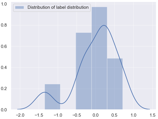
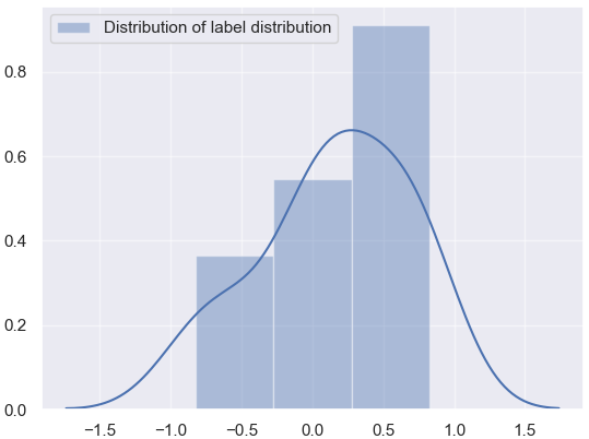
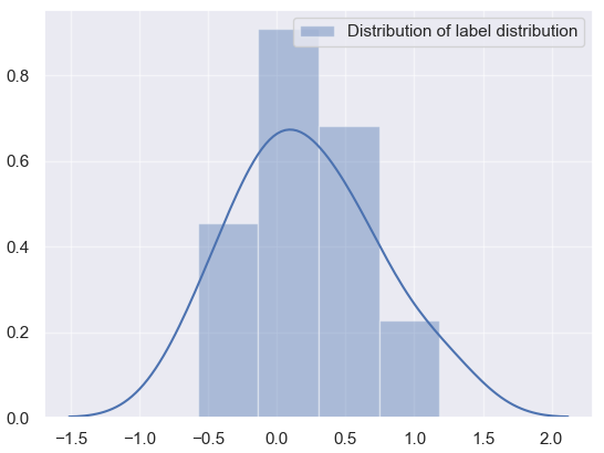
(a) L1 of the matrix	(b) L2 of the matrix	(c) L3 of the matrix
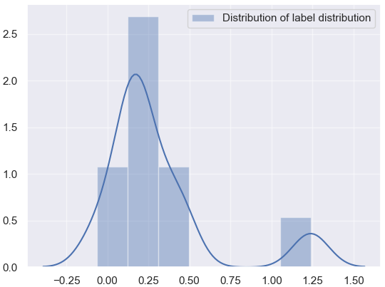
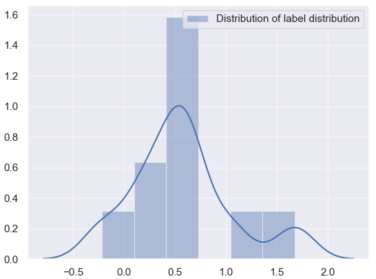
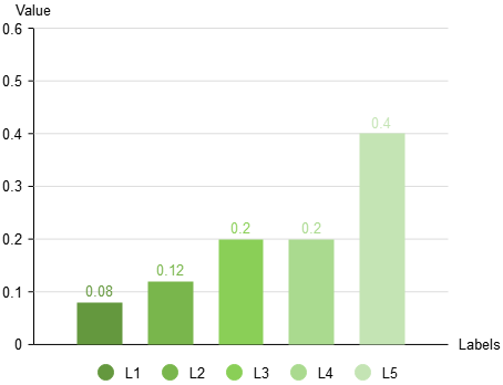
(d) L4 of the matrix	(e) L5 of the matrix	(f) Label distribution

Figure 2: This figure shows the distribution of data for each vector of the label distribution matrix and the corresponding label for this label distribution matrix.

4 Application and Energy Consumption

We select the algorithm executed on Gene as the evaluation model. The evaluation model is conducted on three platforms (lynxi HP300, Raspberry Pi, and Apple smartphones) to check the energy consumption with the same number of iterations (the power is evaluated thanks to the adb script (Dzhagaryan et al. (2016))). Specifically, our model is trained on Gene with the accuracy of float16. Then, the baseline model (MLP replaces SNN and GNN) and our model run inference on a mobile platform, each model executing 500 epochs with 32 batch sizes in the iteration. Experimental results show that our algorithm saves 34.6%, 41.2%, and 40.8% energy compared to the baseline algorithm on the three platforms, respectively.

5 Related Works

Label distribution Learning.

Label distribution learning has attracted several attention as a new learning paradigm. Label distribution learning comes from the scheme proposed by (Geng (2016)) to address the age estimation task. Since then a large number of approaches have been proposed, such as low-rank hypothesis-based (Jia et al. (2019); Ren et al. (2019b)), metric-based (Gao et al. (2018)), manifold-based (Wang & Geng (2021)), and label correlation-based (Teng & Jia (2021); Qian et al. (2022)). Among them, some approaches are executed in computer vision (Chen et al. (2021a)), and speech recognition (Si et al. (2022)) tasks to improve the performance of classifiers. In this paper, we try to build a distribution of label distributions to moderate noise and uncertainty.

Implicit Neural Representations. In implicit neural representation, an object is usually represented as a multi-layer perception (MLP) that maps coordinates to a signal. This idea has been widely applied in modeling 3D object shapes (Lin et al. (2020); Kohli et al. (2020)), 3D surfaces of the scene (Sitzmann et al. (2019); Yariv et al. (2020); Niemeyer et al. (2020); Jiang et al. (2020)), the appearance of the 3D structure as well as the 2D image enhancement (Skorokhodov et al. (2021); Chen et al. (2021b); Anokhin et al. (2021); Karras et al. (2021)). In this paper, we seek to explore this technique to address the label distribution learning issue.

6 Conclusion

In this paper, we design an implicit distribution representation algorithm to moderate the uncertainty of the label values, where the implicit function can be a good estimate of the continuous distribution space. Furthermore, Gaussian prior methods and self-attention mechanisms help the model learn both local signals and global information of the label distribution matrix. Numerous experiments have verified the effectiveness of our approach as well as the suitability of the regularization technique. The application session demonstrates the high efficiency of our proposed model.

References

- Anokhin et al. (2021) Ivan Anokhin, Kirill Demochkin, Taras Khakhulin, Gleb Sterkin, Victor Lempitsky, and Denis Korzhenkov. Image generators with conditionally-independent pixel synthesis. In CVPR, 2021.
- Chen et al. (2021a) Jingying Chen, Chen Guo, Ruyi Xu, Kun Zhang, Zongkai Yang, and Honghai Liu. Toward children’s empathy ability analysis: Joint facial expression recognition and intensity estimation using label distribution learning. IEEE Transactions on Industrial Informatics, 2021a.
- Chen et al. (2021b) Yinbo Chen, Sifei Liu, and Xiaolong Wang. Learning continuous image representation with local implicit image function. In CVPR, 2021b.
- Deng et al. (2020) Jiankang Deng, Jia Guo, Evangelos Ververas, Irene Kotsia, and Stefanos Zafeiriou. Retinaface: Single-shot multi-level face localisation in the wild. In CVPR, 2020.
- Dzhagaryan et al. (2016) Armen Dzhagaryan, Aleksandar Milenkovic, Mladen Milosevic, and Emil Jovanov. An environment for automated measuring of energy consumed by android mobile devices. In PECCS, 2016.
- Escalera et al. (2015) Sergio Escalera, Junior Fabian, Pablo Pardo, Xavier Baró, Jordi Gonzalez, Hugo J Escalante, Dusan Misevic, Ulrich Steiner, and Isabelle Guyon. Chalearn looking at people 2015: Apparent age and cultural event recognition datasets and results. In ICCVW, 2015.
- Gao et al. (2017) Bin-Bin Gao, Chao Xing, Chen-Wei Xie, Jianxin Wu, and Xin Geng. Deep label distribution learning with label ambiguity. IEEE TIP, 2017.
- Gao et al. (2018) Bin-Bin Gao, Hong-Yu Zhou, Jianxin Wu, and Xin Geng. Age estimation using expectation of label distribution learning. In IJCAI, 2018.
- Geng (2016) Xin Geng. Label distribution learning. IEEE TKDE, 2016.
- Ghosh et al. (2021) Aishik Ghosh, Benjamin Nachman, and Daniel Whiteson. Uncertainty-aware machine learning for high energy physics. Physical Review D, 2021.
- He et al. (2015) Kaiming He, Xiangyu Zhang, Shaoqing Ren, and Jian Sun. Delving deep into rectifiers: Surpassing human-level performance on imagenet classification. In ICCV, 2015.
- Hu et al. (2021) Zijian Hu, Zhengyu Yang, Xuefeng Hu, and Ram Nevatia. Simple: similar pseudo label exploitation for semi-supervised classification. In CVPR, 2021.
- Jia et al. (2019) Xiuyi Jia, Xiang Zheng, Weiwei Li, Changqing Zhang, and Zechao Li. Facial emotion distribution learning by exploiting low-rank label correlations locally. In CVPR, 2019.
- Jia et al. (2021a) Xiuyi Jia, Xiaoxia Shen, Weiwei Li, Yunan Lu, and Jihua Zhu. Label distribution learning by maintaining label ranking relation. IEEE TKDE, 2021a.
- Jia et al. (2021b) Xiuyi Jia, Tao Wen, Weiping Ding, Huaxiong Li, and Weiwei Li. Semi-supervised label distribution learning via projection graph embedding. Information Sciences, 2021b.
- Jiang et al. (2020) Chiyu Jiang, Avneesh Sud, Ameesh Makadia, Jingwei Huang, Matthias Nießner, Thomas Funkhouser, et al. Local implicit grid representations for 3D scenes. In CVPR, 2020.
- Johnson et al. (2016) Justin Johnson, Alexandre Alahi, and Li Fei-Fei. Perceptual losses for real-time style transfer and super-resolution. In ECCV, 2016.
- Ju et al. (2019) Mingye Ju, Can Ding, Y Jay Guo, and Dengyin Zhang. Idgcp: Image dehazing based on gamma correction prior. IEEE TIP, 2019.
- Karras et al. (2021) Tero Karras, Miika Aittala, Samuli Laine, Erik Härkönen, Janne Hellsten, Jaakko Lehtinen, and Timo Aila. Alias-free generative adversarial networks. In NeurIPS, 2021.
- Kohli et al. (2020) Amit Kohli, Vincent Sitzmann, and Gordon Wetzstein. Inferring semantic information with 3D neural scene representations. arXiv preprint arXiv:2003.12673, 2020.
- Li et al. (2022) Qiang Li, Jingjing Wang, Zhaoliang Yao, Yachun Li, Pengju Yang, Jingwei Yan, Chunmao Wang, and Shiliang Pu. Unimodal-concentrated loss: Fully adaptive label distribution learning for ordinal regression. In CVPR, 2022.
- Lin et al. (2020) Chen-Hsuan Lin, Chaoyang Wang, and Simon Lucey. SDF-SRN: Learning signed distance 3D object reconstruction from static images. In NeurIPS, 2020.
- Liu et al. (2021) Tingting Liu, Jixin Wang, Bing Yang, and Xuan Wang. Ngdnet: Nonuniform gaussian-label distribution learning for infrared head pose estimation and on-task behavior understanding in the classroom. Neurocomputing, 2021.
- Niemeyer et al. (2020) Michael Niemeyer, Lars Mescheder, Michael Oechsle, and Andreas Geiger. Differentiable volumetric rendering: Learning implicit 3D representations without 3D supervision. In CVPR, 2020.
- Northcutt et al. (2021) Curtis Northcutt, Lu Jiang, and Isaac Chuang. Confident learning: Estimating uncertainty in dataset labels. Journal of Artificial Intelligence Research, 2021.
- Patel et al. (2021) Kinjal Patel, Eric Hunsberger, Sean Batir, and Chris Eliasmith. A spiking neural network for image segmentation. arXiv preprint arXiv:2106.08921, 2021.
- Qian et al. (2022) Wenbin Qian, Yinsong Xiong, Jun Yang, and Wenhao Shu. Feature selection for label distribution learning via feature similarity and label correlation. Information Sciences, 2022.
- Qin et al. (2022) Zhen Qin, Weixuan Sun, Hui Deng, Dongxu Li, Yunshen Wei, Baohong Lv, Junjie Yan, Lingpeng Kong, and Yiran Zhong. cosformer: Rethinking softmax in attention. In ICLR, 2022.
- Ren et al. (2019a) Tingting Ren, Xiuyi Jia, Weiwei Li, Lei Chen, and Zechao Li. Label distribution learning with label-specific features. In IJCAI, 2019a.
- Ren et al. (2019b) Tingting Ren, Xiuyi Jia, Weiwei Li, and Shu Zhao. Label distribution learning with label correlations via low-rank approximation. In IJCAI, 2019b.
- Ricanek & Tesafaye (2006) Karl Ricanek and Tamirat Tesafaye. Morph: A longitudinal image database of normal adult age-progression. In FGR06, 2006.
- Si et al. (2022) Shijing Si, Jianzong Wang, Junqing Peng, and Jing Xiao. Towards speaker age estimation with label distribution learning. In ICASSP, 2022.
- Sitzmann et al. (2019) Vincent Sitzmann, Michael Zollhöfer, and Gordon Wetzstein. Scene representation networks: Continuous 3D-structure-aware neural scene representations. In NeurIPS, 2019.
- Sitzmann et al. (2020) Vincent Sitzmann, Julien Martel, Alexander Bergman, David Lindell, and Gordon Wetzstein. Implicit neural representations with periodic activation functions. In NeurIPS, 2020.
- Skorokhodov et al. (2021) Ivan Skorokhodov, Savva Ignatyev, and Mohamed Elhoseiny. Adversarial generation of continuous images. In CVPR, 2021.
- Teng & Jia (2021) Qifa Teng and Xiuyi Jia. Incomplete label distribution learning by exploiting global sample correlation. In Multimedia Understanding with Less Labeling on Multimedia Understanding with Less Labeling. 2021.
- Ucar et al. (2021) Talip Ucar, Ehsan Hajiramezanali, and Lindsay Edwards. Subtab: Subsetting features of tabular data for self-supervised representation learning. In NeurIPS, 2021.
- Vaswani et al. (2017) Ashish Vaswani, Noam Shazeer, Niki Parmar, Jakob Uszkoreit, Llion Jones, Aidan N Gomez, Łukasz Kaiser, and Illia Polosukhin. Attention is all you need. In NeurIPS, 2017.
- Wang & Geng (2021) Jing Wang and Xin Geng. Label distribution learning by exploiting label distribution manifold. IEEE TNNLS, 2021.
- Wortsman et al. (2022) Mitchell Wortsman, Gabriel Ilharco, Samir Ya Gadre, Rebecca Roelofs, Raphael Gontijo-Lopes, Ari S Morcos, Hongseok Namkoong, Ali Farhadi, Yair Carmon, Simon Kornblith, et al. Model soups: averaging weights of multiple fine-tuned models improves accuracy without increasing inference time. In ICML, 2022.
- Xu et al. (2019) Ning Xu, Yun-Peng Liu, and Xin Geng. Label enhancement for label distribution learning. IEEE TKDE, 2019.
- Xu et al. (2020) Ning Xu, Jun Shu, Yun-Peng Liu, and Xin Geng. Variational label enhancement. In ICML, 2020.
- Yamazaki et al. (2022) Kashu Yamazaki, Viet-Khoa Vo-Ho, Darshan Bulsara, and Ngan Le. Spiking neural networks and their applications: A review. Brain Sciences, 2022.
- Yang et al. (2021) Jiancheng Yang, Rui Shi, and Bingbing Ni. Medmnist classification decathlon: A lightweight automl benchmark for medical image analysis. In ISBI, 2021.
- Yariv et al. (2020) Lior Yariv, Yoni Kasten, Dror Moran, Meirav Galun, Matan Atzmon, Basri Ronen, and Yaron Lipman. Multiview neural surface reconstruction by disentangling geometry and appearance. 2020.
- Zhang et al. (2018) Hongyi Zhang, Moustapha Cisse, Yann N Dauphin, and David Lopez-Paz. Mixup: Beyond empirical risk minimization. In ICLR, 2018.
- Zhao & Zhou (2018) Peng Zhao and Zhi-Hua Zhou. Label distribution learning by optimal transport. In AAAI, 2018.
- Zhao et al. (2022) Xingyu Zhao, Yuexuan An, Ning Xu, and Xin Geng. Fusion label enhancement for multi-label learning. In IJCAI, 2022.
- Zhao et al. (2021) Zengqun Zhao, Qingshan Liu, and Feng Zhou. Robust lightweight facial expression recognition network with label distribution training. In AAAI, 2021.
- Zheng et al. (2021a) Qinghai Zheng, Jihua Zhu, Haoyu Tang, Xinyuan Liu, Zhongyu Li, and Huimin Lu. Generalized label enhancement with sample correlations. IEEE TKDE, 2021a.
- Zheng et al. (2021b) Rui Zheng, Shulin Zhang, Lei Liu, Yuhao Luo, and Mingzhai Sun. Uncertainty in bayesian deep label distribution learning. Applied Soft Computing, 2021b.