Online Multi Camera-IMU Calibration

Abstract

Visual-inertial navigation systems are powerful in their ability to accurately estimate localization of mobile systems within complex environments that preclude the use of global navigation satellite systems. However, these navigation systems are reliant on accurate and up-to-date temporospatial calibrations of the sensors being used. As such, online estimators for these parameters are useful in resilient systems. In this paper, we present an extension to existing Kalman Filter based frameworks for estimating and calibrating the extrinsic parameters of IMU and multi-camera systems. In addition to extended the filter framework to include multiple camera sensors, we reformulate the measurement model to make use of measurement data that is typically available in fiducial detection software. Finally, we include a secondary set of filters that estimate the time translation parameters without closed-loop feedback. Experimental calibration results, including cameras with non-overlapping fields of view. Finally the code has been open-sourced and made available.

I Introduction

For any mobile robotic system, localization is key to the success of a mission. The ability for a vehicle or robot to precisely determine its location within a local reference frame is paramount to the subsequent problems of navigation, path planning, and control. Historically, high accuracy localization was achieved using a combination of an Inertial Measurement Unit (IMU) and a Global Navigation Satellite System (GNSS), colloquially referred to as GPS. The success of this combination of sensors came from the high update rates achievable by IMUs with relatively good accuracy over short time periods, and the zero drift corrections coming from the GPS.

Unfortunately, GPS aided navigation is often unavailable or inaccurate due to environmental factors. Any system that is indoors, underwater, or surrounded by tall buildings would be unable to reliably use GPS for localization. Additionally, high accuracy GPS receivers are often too large and expensive to deploy in large numbers for small robotics. Comparatively, cameras are lightweight, inexpensive, and provide rich environmental information. As such, Visual Inertial Navigation Systems (V-INS) have sought to leverage the robust information and combine these measurements with inertial sensors to provide high speed and high accuracy localization [1, 2].

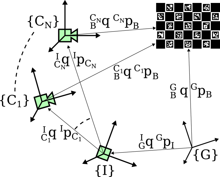
Figure 1: Relationship graph between frames of reference showing translations and rotations between the Global {$G$}, Board {$B$}, IMU {$I$}, and Camera {$C_{1}$…$C_{N}$} frames

For a V-INS to work properly, it is necessary to accurately calibrate camera IMU systems for high-accuracy localization. Methods for performing this calibration include the use of high accuracy 3D measurements using CAD models or 3D scanners. However, these methods can be prohibitive due to cost and resource constraints. Additionally, without further calibration of the physical sensor body with the produced measurements, these types of calibrations cannot fully calculate the extrinsic calibration parameters. Finally, due to shifts in sensor mounting, maintenance, or repair, calibrations cannot be assumed to be constant over the lifetime of a mobile system, further increasing the costs of calibration.

Because of these limitations, offline batch optimization has often been used to calibrate systems using measurement data in a defined environment. This method can produce accurate extrinsic and temporal calibration parameters of camera-IMU systems with very little cost [3, 4, 5]. However, this calibration must be done as a non-sequential batch process which would struggle with estimating parameters over a large time scale. Additionally, batch processes by their nature are unable to handle sudden changes to sensor extrinsics, such as a sensor shifts due to disturbance or vibration.

As such, online calibrations using Extended Kalman Filter (EKF) frameworks have been used to calibrate camera-IMU systems [6, 7, 8, 9, 10]. These Kalman filter based methods can perform online calibrations as well as handle step changes to sensor extrinsic parameters. In this paper, we present an update to the EKF-based algorithm for IMU-camera system calibration that incorporates multiple cameras. This framework adapts existing measurement models to take advantage of open source computer vision software for the detection of visual fiducials, which can lead to decreased developmental complexity and simplify the filter measurement update. We also provide an example of this framework through the open-sourced repository found at [11]. Finally, we consider temporal calibration through the development of a simple one way time translation filter that can be applied to any sensor measurement that does not utilize two-way clock synchronization.

II Related Work

The IMU and single camera calibration filter that this paper extends and adapts was originally proposed and implemented in [6]. Reformulations of this filter have been successfully implemented using unscented Kalman filters [12, 13] or a multi-state constraint Kalman filter [7]. We extend the results of what has been previously performed through the experimental use of multiple cameras with differing data transmission types and rates, as well as the use of quaternion measurements in the camera update function. This is done because ArUco markers can be assumed to be a 3D pose sensor with low error in both relative position and orientation [14]. This sensing model is used in place of the 2D projective model previously used in other online filter frameworks [6]. This was done to show how any fiducial marker that satisfies the simplifying assumption of being a robust 3D sensor could be used to quickly incorporate a camera into a localization filter.

Calibration checkerboards are often used for their subpixel accuracy when calibrating camera intrinsics. Combining checkerboards with fiducials such as ArUco markers these two in the form of ChArUco markers allows for subpixel accuracy as well as the discerning of 180 degree rotations. The added simplicity of using open source fiducial marker detection packages such as OpenCV allows for rapid development [15]. As such, we also show that it is possible to make use of more complex fiducials that can offer more accurate measurements than simple feature tracking. By taking any existing fiducial detector, the framework described in this work is capable of quickly adopting any number styles of marker and associated detectors.

The calibration of proprioceptive and exteroceptive sensors is often considered a spatial problem, where intrinsic properties are calculated separately from the extrinsic, and the main concern is in determining a translation vector and rotation matrix. This manifests in work where the goal is to determine these extrinsic parameters either through online or offline methods [16, 17]. However, the calibration problem is not purely spatial, but rather temporospatial inasmuch as it is necessary to know the location, orientation and time which a measurement was taken in order to properly include in a filter in an optimal way. As such, work has been done to more rigorously calibrate sensors temporally using both offline and online methods [13]. Additionally, the relative importance of accurate time measurements has been shown to have significant impacts on exteroceptive sensors such as cameras [18]. While others have solved this temporospatial calibration by including the time translation into the Kalman state vector, we propose a sub-filter methodology, that is not reliant on state updates to correct sensor timings. This can be applied to any sensor that cannot take advantage of closed loop synchronization systems such as Precision Time Protocol (PTP) or where hardware time synchronization is either difficult or impossible to achieve with given sensor hardware [19].

III Algorithm Description

The filter state is composed of a singular IMU state and multiple independent camera states represented by $\boldsymbol{x}_{imu}$ and $\boldsymbol{x}_{cam_{i}}$ respectively. The IMU state contains the rotation of the global frame in the IMU frame $\prescript{I}{G}{q}$, the gyroscope bias $\mathbf{}{\mathbf{b}}_{g}$, the imu velocity in the global frame $\prescript{G}{}{\mathbf{v}}_{I}$, the accelerometer bias $\mathbf{b}_{a}$, and the imu position in the global frame $\prescript{G}{}{\mathbf{p}}_{I}$. Additionally, each camera state is composed of the orientation in the IMU frame $\prescript{I}{C}{q}$, and the position in the IMU frame $\prescript{I}{}{\mathbf{p}}_{C}$. Shown in Figure 1 are the relative frames for the Global {$G$}, Calibration Board {$B$}, IMU {$I$}, and Cameras {$C_{1}$}…{$C_{N}$}. Additionally shown are the inter-frame translations and rotations $p$ and $q$, respectively. Therefore, the entire state matrix with $N$ cameras is

$$\boldsymbol{x}=\begin{bmatrix}\boldsymbol{x}_{imu}&\boldsymbol{x}_{cam_{1}}&...&\boldsymbol{x}_{cam_{N}}\end{bmatrix}^{T}$$ (1)

where

$$\boldsymbol{x}_{imu}=\begin{bmatrix}\prescript{I}{G}{q}&\mathbf{}{\mathbf{b}}_{g}&\prescript{G}{}{\mathbf{v}}_{I}&\mathbf{b}_{a}&\prescript{G}{}{\mathbf{p}}_{I}\end{bmatrix}$$ (2)

$$\boldsymbol{x}_{cam_{i}}=\begin{bmatrix}\prescript{I}{C}{q}&\prescript{I}{}{\mathbf{p}}_{C}\end{bmatrix}_{i}$$ (3)

III-A One-Way Time Translation

A one-way time translation filter was created using a first order translation model, similar to the formation in [18]. We assume the map from the measured sensor time $t_{s}$ to the computer time $t_{c}$ is linear with a skew $\alpha$ and offset $\beta$.

$$t_{c}=\alpha\cdot t_{s}+\beta$$ (4)

With this model, the filter state is composed of the translation equation coefficients

$$\mathbf{x}=\begin{bmatrix}\alpha&\beta\end{bmatrix}^{T}$$ (5)

We initialize the filter using the initial sensor time $t_{c_{0}}$ and initial main computer time $t_{c_{0}}$.

$$\mathbf{x}_{0}=\begin{bmatrix}1\\ t_{c_{0}}-t_{s_{0}}\end{bmatrix}$$ (6)

The measurement $z$ and measurement model $\hat{z}$ are simply

$$z=t_{c_{0}}-t_{s_{0}}$$ (7)

$$\hat{z}=\alpha\cdot t_{s}+\beta$$ (8)

Therefore, the observation matrix is

$$\mathbf{H}=\begin{bmatrix}t_{s}&1\end{bmatrix}$$ (9)

With these definitions, the typical EKF equations are used to update the filter state and covariance. Using the filter state values with Equation 4 gives an estimate of the measurement time translated to the main computer frame of reference.

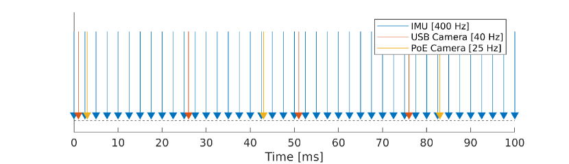
Figure 2: Sensor update rates used in the experimental work

These filters were created outside the main calibration filter in this work due to a number of reasons. First, because the highly uncorrelated nature of the timing measurements from different sensors, it would unnecessarily increase the complexity of the filter to include each $\alpha$ and $\beta$ parameter for every sensor using time translation. Additionally, this method allows for greater flexibility of the applied time-translation filter. In the case of this work, one camera utilized PTP while the other utilized a time-translation filter with update rates outlined in Figure 2. As such, the separation of the filters allows the extrinsic camera parameters to be vectorized in the main filter. Finally, because the time a sensor measurement is taken is relevant to the update it provides, this method provides updated sensor measurement time before it is used within the main calibration filter.

III-B Calibration State Initialization

The filter state is initialized using initial estimates of the extrinsic parameters and the first update. The initial extrinsic parameter estimates can come from any calibration source. The IMU pose is initialized upon the first successful camera measurement of $(\prescript{B}{}{\mathbf{p}}_{C},~{}\prescript{B}{C}{q})$ as follows

$$\begin{split}\prescript{I}{G}{\hat{q}}&=(\prescript{G}{B}{q}\otimes\prescript{B}{C}{q}\otimes\prescript{C}{I}{\hat{q}})^{-1}\\ \prescript{G}{}{\hat{\mathbf{p}}}_{I}&=\prescript{G}{}{\mathbf{p}}_{C}+\prescript{G}{}{\mathbf{p}}_{B}-\mathcal{C}(\prescript{I}{G}{\hat{q}})^{T}\prescript{I}{}{\mathbf{p}}_{C}\end{split}$$ (10)

where $\mathcal{C}(q)$ represents the rotation matrix corresponding to quaternion $q$ and $\otimes$ represents quaternion multiplication.

III-C Calibration State Propagation

As shown in [6], we can apply the expectation operator to the continuous-time dynamics of the system, and produce the following state propagation equations. The only notable difference is the expansion of these propagation equations to include multiple cameras, denoted by the subscript $N$ for each camera reference frame $C$.

$$\prescript{I}{G}{\dot{\hat{q}}}(t) =\frac{1}{2}\Omega(\hat{\boldsymbol{\omega}}(t))\prescript{I}{G}{\hat{q}}(t)$$ (11)

$$\dot{\hat{\mathbf{b}}}_{g}(t) =\mathbf{0}_{3\times 1}$$ (12)

$$\prescript{G}{}{\dot{\hat{\mathbf{v}}}}_{I}(t) =\boldsymbol{C}^{T}(\prescript{I}{G}{\hat{q}}(t))\prescript{G}{}{\hat{\mathbf{a}}}(t)+\prescript{G}{}{\mathbf{g}}$$ (13)

$$\dot{\hat{\mathbf{b}}}_{a}(t) =\mathbf{0}_{3\times 1}$$ (14)

$$\prescript{G}{}{\dot{\hat{\mathbf{p}}}}_{I}(t) =\prescript{G}{}{\hat{\mathbf{v}}}_{I}(t)$$ (15)

$$\prescript{I}{{C_{N}}}{\dot{\hat{q}}}(t) =\mathbf{0}_{3\times 1}$$ (16)

$$\prescript{I}{}{\dot{\mathbf{p}}}_{C_{N}}(t) =\mathbf{0}_{3\times 1}$$ (17)

By integrating Equations 11, 12, 13, 14, 15, 16 and 17, a propagated state estimate is produced in discrete time. However, in order to propagate the state covariance, an error state filter using multiple cameras is used where the error state is

$$\boldsymbol{\widetilde{x}}=\begin{bmatrix}\boldsymbol{\widetilde{x}}_{imu}&\boldsymbol{\widetilde{x}}_{cam_{1}}&...&\boldsymbol{\widetilde{x}}_{cam_{N}}\end{bmatrix}^{T}$$ (18)

where

$$\boldsymbol{\widetilde{x}}_{imu}=\begin{bmatrix}\prescript{I}{G}{\delta\theta}&\widetilde{\mathbf{b}}_{g}&\prescript{G}{}{\widetilde{\mathbf{v}}}_{I}&\widetilde{\mathbf{b}}_{a}&\prescript{G}{}{\widetilde{\mathbf{p}}}_{I}\end{bmatrix}$$ (19)

$$\boldsymbol{\widetilde{x}}_{cam_{i}}=\begin{bmatrix}\prescript{I}{C}{\delta\theta}&\prescript{G}{}{\widetilde{\mathbf{p}}}_{C}\end{bmatrix}_{i}$$ (20)

The linearized continuous-time error-state propagation is given by

$$\dot{\widetilde{\mathbf{x}}}=\mathbf{F}\widetilde{\mathbf{x}}+\mathbf{G}\mathbf{n}$$ (21)

where for N cameras

$$\mathbf{F}=\begin{bmatrix}-\left[\hat{\boldsymbol{\omega}}\times\right]&-\mathbf{I}_{3}&\mathbf{0}_{3\times 3}&\mathbf{0}_{3\times 3}&\mathbf{0}_{3\times 9}\\ \mathbf{0}_{3\times 3}&\mathbf{0}_{3\times 3}&\mathbf{0}_{3\times 3}&\mathbf{0}_{3\times 3}&\mathbf{0}_{3\times 9}\\ \mathcal{C}(\prescript{I}{G}{\hat{q}})\left[\hat{\mathbf{a}}\times\right]&\mathbf{0}_{3\times 3}&\mathbf{0}_{3\times 3}&-\mathcal{C}(\prescript{I}{G}{\hat{q}})^{T}&\mathbf{0}_{3\times 9}\\ \mathbf{0}_{3\times 3}&\mathbf{0}_{3\times 3}&\mathbf{0}_{3\times 3}&\mathbf{0}_{3\times 3}&\mathbf{0}_{3\times 9}\\ \mathbf{0}_{3\times 3}&\mathbf{0}_{3\times 3}&\mathbf{I}_{3}&\mathbf{0}_{3\times 3}&\mathbf{0}_{3\times 9}\\ \mathbf{0}_{6N\times 3}&\mathbf{0}_{6N\times 3}&\mathbf{0}_{6N\times 3}&\mathbf{0}_{6N\times 3}&\mathbf{0}_{6N\times 9}\\ \end{bmatrix}$$

$$\mathbf{G}=\begin{bmatrix}-\mathbf{I}_{3}&\mathbf{0}_{3\times 3}&\mathbf{0}_{3\times 3}&\mathbf{0}_{3\times 3}\\ \mathbf{0}_{3\times 3}&\mathbf{I}_{3}&\mathbf{0}_{3\times 3}&\mathbf{0}_{3\times 3}\\ \mathbf{0}_{3\times 3}&\mathbf{0}_{3\times 3}&-\mathcal{C}(\prescript{I}{G}{\hat{q}})&\mathbf{0}_{3\times 3}\\ \mathbf{0}_{3\times 3}&\mathbf{0}_{3\times 3}&\mathbf{0}_{3\times 3}&\mathbf{I}_{3}\\ \mathbf{0}_{3\times 3}&\mathbf{I}_{3}&\mathbf{0}_{3\times 3}&\mathbf{0}_{3\times 3}\\ \mathbf{0}_{6N\times 3}&\mathbf{0}_{6N\times 3}&\mathbf{0}_{6N\times 3}&\mathbf{0}_{6N\times 3}\\ \end{bmatrix},~{}\mathbf{n}=\begin{bmatrix}\mathbf{n}_{g}\\ \mathbf{n}_{wg}\\ \mathbf{n}_{a}\\ \mathbf{n}_{wa}\end{bmatrix}$$

and the cross product operator is defined as

$$\left[\boldsymbol{\omega}\times\right]\equiv\begin{bmatrix}0&-\omega_{z}&-\omega_{y}\\ \omega_{z}&0&-\omega_{x}\\ -\omega_{y}&\omega_{x}&0\end{bmatrix}$$ (22)

The remaining derivations are consistent with the typical development of an error state Kalman filter which is well described in [20].

III-D Measurement Model

The cameras, which are rigidly attached to the IMU, record images of a calibration target where the target frame has a known location and orientation within the global frame $\prescript{G}{}{\mathbf{p}}_{B}$ and $\prescript{B}{G}{q}$ respectively. Using a calibration target such as a grid board of April tags or a ChArUco board, it is possible to use the estimatePoseBoard() function from OpenCV to extract translation and rotation vectors in the target frame [15]. Therefore, the measurement model for each camera is simply

$$\mathbf{z}=\begin{bmatrix}\prescript{B}{}{\mathbf{p}}_{C}\\ \prescript{B}{C}{q}\end{bmatrix}$$ (23)

$$\hat{\mathbf{z}}=\begin{bmatrix}\mathcal{C}(\prescript{B}{G}{q})(\prescript{G}{}{\hat{\mathbf{p}}}_{I}-\prescript{G}{}{\mathbf{p}}_{B}+\mathcal{C}(\prescript{B}{G}{\hat{q}})\prescript{I}{}{\hat{\mathbf{p}}}_{C})\\ \prescript{I}{C}{\hat{q}}^{-1}\otimes\prescript{I}{G}{\hat{q}}\otimes\prescript{B}{G}{q}^{-1}\end{bmatrix}$$ (24)

The measurement matrix for the first camera is

$$\mathbf{H}=\begin{bmatrix}\mathbf{\prescript{p}{}{J}}_{\prescript{I}{G}{q},p}&\mathbf{0}_{3\times 9}&\mathbf{J}_{\prescript{G}{}{p}_{I}}&\mathbf{\prescript{p}{}{J}}_{\prescript{I}{C}{q}}&\mathbf{J}_{\prescript{I}{C}{p}}&\mathbf{0}_{3\times 6}\\ \mathbf{\prescript{q}{}{J}}_{\prescript{I}{G}{q},q}&\mathbf{0}_{3\times 9}&\mathbf{0}_{3\times 3}&\mathbf{\prescript{q}{}{J}}_{\prescript{i}{C}{q}}&\mathbf{0}_{3\times 3}&\mathbf{0}_{3\times 6}\end{bmatrix}$$ (25)

and for the second camera is

$$\mathbf{H}=\begin{bmatrix}\mathbf{\prescript{p}{}{J}}_{\prescript{I}{G}{q},p}&\mathbf{0}_{3\times 9}&\mathbf{J}_{\prescript{G}{}{p}_{I}}&\mathbf{0}_{3\times 6}&\mathbf{\prescript{p}{}{J}}_{\prescript{I}{C}{q}}&\mathbf{J}_{\prescript{I}{C}{p}}\\ \mathbf{\prescript{q}{}{J}}_{\prescript{I}{G}{q},q}&\mathbf{0}_{3\times 9}&\mathbf{0}_{3\times 3}&\mathbf{0}_{3\times 6}&\mathbf{\prescript{q}{}{J}}_{\prescript{i}{C}{q}}&\mathbf{0}_{3\times 3}\end{bmatrix}tem$$ (26)

where

$$\mathbf{\prescript{p}{}{J}}_{\prescript{I}{G}{q}} =-\mathcal{C}(\prescript{I}{C}{q})^{T}\mathcal{C}(\prescript{I}{G}{q})\left[\prescript{G}{}{p}_{B}-\prescript{G}{}{p}_{I}\times\right]\mathcal{J}(\prescript{I}{G}{q},)$$ (27)

$$\mathbf{J}_{\prescript{G}{}{p}_{I}} =-\mathcal{C}(\prescript{I}{C}{q})^{T}\mathcal{C}(\prescript{I}{G}{q})$$ (28)

$$\mathbf{\prescript{p}{}{J}}_{\prescript{I}{C}{q}} =-\mathcal{C}(\prescript{I}{C}{q})^{T}\left[\mathcal{C}(\prescript{I}{G}{q})*(\prescript{G}{}{p}_{B}-\prescript{G}{}{p}_{I})-\prescript{I}{}{p}_{C}\times\right]$$ (29)

$$\mathbf{J}_{\prescript{I}{C}{p}} =-\mathcal{C}(\prescript{I}{C}{q})^{T}$$ (30)

Note that the Jacobians $\mathbf{J}_{\prescript{I}{G}{q},p}$ and $\mathbf{J}_{\prescript{I}{C}{q},q}$ are not reproduced here due to the complexity of the analytical solution. In practice, the use of numerical solutions for these jacobians is simpler and computationally faster. Additionally, these Jacobians are not taken with respect to the measurement $\hat{z}$ due to the singularity at the 180 degree rotation mark. Rather, we take the Jacobian of the residual $\hat{z}-z$ which produces much smaller measurements, as is expected with an error state Kalman filter formulation. These smaller measurements produce more linear and stable results when the system experiences large rotations.

Moreover, the structure of this filter allows for N cameras by adjusting the column location of the measurement matrix as shown in Equations 25 and 26 and is therefore quite extensible in both analysis and in software.

III-E Calibration Measurement Update

Using the measurement model outlined in Section III-D, we apply the usual Kalman update equations

$$\mathbf{y}=\mathbf{z}-\hat{\mathbf{z}}$$ (31)

$$\mathbf{S}=\mathbf{H}\mathbf{P}\mathbf{H}^{T}+\mathbf{R}$$ (32)

$$\mathbf{K}=\mathbf{P}\mathbf{H}^{T}\mathbf{S}^{-1}$$ (33)

The Mahalanobis distance is calculated to reject outliers that exceed a probabilistic threshold

$$\chi^{2}=\mathbf{y}^{T}\mathbf{S}^{-1}\mathbf{y}$$ (34)

Measurements that pass the threshold test are used to update the state

$$\hat{\mathbf{x}}=\hat{\mathbf{x}}\oplus\mathbf{K}\mathbf{y}$$ (35)

Where the state composition $\oplus$ is defined as addition for vectors and quaternion multiplication for quaternions. Additionally, the covariance update is computed with the following

$$\mathbf{P}=(\mathbf{I}-\mathbf{K}\mathbf{H})\mathbf{P}(\mathbf{I}-\mathbf{K}\mathbf{H})^{T}+\mathbf{K}\mathbf{R}\mathbf{K}^{T}$$ (36)

Known as the Joseph form, it is used for it’s balance of improved numerical stability with computational complexity [21].

IV Experimental Results

IV-A One-Way Time Filtering

For both the VectorNav IMU and the Basler Ace camera, we implemented the one-way time translation filter in order to improve the inconsistent time measurements. The two-parameter filter converges quickly for both parameters. This led to rapid reduction in noise reported in the sensor measurements, with convergence to the expected measurement frequency, as shown in Figure 3. Similar convergence of the parameters and the measurement time step for the USB camera were observed. Specifically, the translated measurement period settled within 10 $\mu s$ of the reported sensor measurement period in 0.3 seconds for the IMU and 1.0 seconds for the USB camera. Compared to the convergence time on the order of seconds or even minutes seen in PTP filters, we believe this is a reasonable translation convergence time to see.

Due to the convergence in the differences of the sensor time output in each the USB IMU and camera, we find that the application of this one-way time filter to be useful in rejecting the noise that can appear when using non-networked sensors. Additionally, due to the low overhead of the calculations, even high rate sensors, such as IMUs, can use this filter without substantial reductions in throughput.

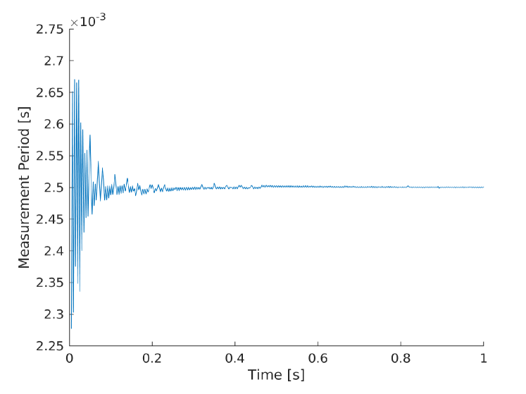
Figure 3: Measurement period translated from sensor time shown converging to 400 Hz ($2.5\times 10^{-3}$ seconds)

IV-B Multi-Camera EKF Results with Visual Overlap

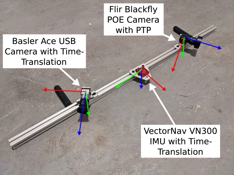
Figure 4: Mounting system used to test multi-camera IMU calibration with configuration showing non-overlapping fields of view

To validate the efficacy of the filter design, we used a multi-camera IMU rig that is capable of rigidly mounting cameras and an IMU in various setups shown in Figure 4. Using this rig, it was possible to test the filter using both PoE and USB 3.0 cameras and differing rates.

Using a stationary ChArUco calibration target, data was collected exciting all six degrees of freedom while keeping the calibration pattern in the field of view for both cameras. The time translation filter operated on the USB sensors, and the calibration filter was applied on the sensor output and camera detections using the OpenCV estimatePoseBoard function. We found that the filter consistently converged on sensor extrinsic parameters given the measurements and typically within 20 seconds of the initial detections of the calibration target.

Additionally, it was possible to run the filter with either one of the camera measurement streams. Shown is the convergence of the main axis of offset between the cameras in the IMU frame. In this case, that is the y-axis. Figures 5 and 6 show the convergence of the camera extrinsics when only a single camera is used in the filter. When both cameras are used, shown in Figure 7, the filter converges faster and more consistently. Similar results were seen in the remaining translation and rotation axes.

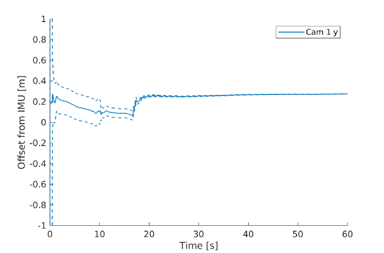
Figure 5: Camera 1 independent y-axis convergence plot

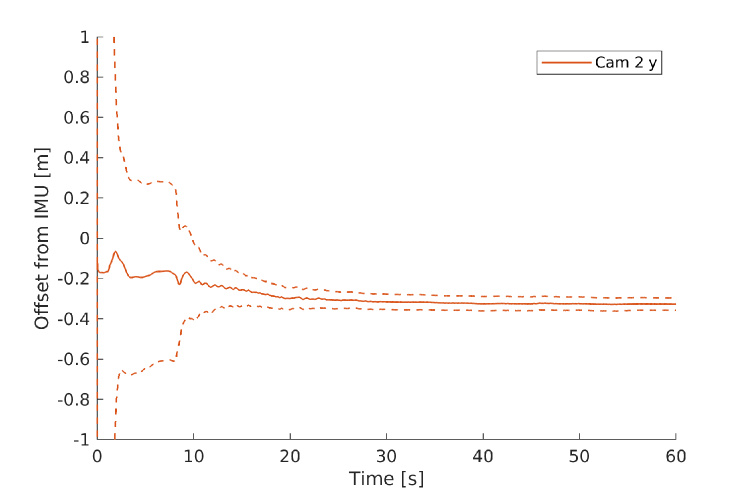
Figure 6: Camera 2 independent y-axis convergence plot

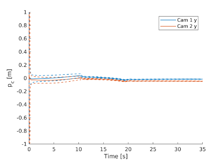
Figure 7: Dual camera y-axis convergence plot with overlapping fields of view

IV-C Filter Evaluation

In order to validate the implementation of our algorithm, we compare our experimental results of with the outputs the MatLab camera calibration toolbox [22]. Using synchronized captures from both cameras, a relative offset was found that could be compared to the output of the filter, shown in Table I. The relative difference between the calibration application and the EKF is quite low, especially with regards to the physical location. We note the Y offset (The direction into the camera frame) had higher error than the other dimensions, which we believe is attributable to the small calibration target used that limited the excitation possible in this direction. With this in mind, we believe the converged filter values to be validated.

TABLE I: Comparison of extrinsic parameters in IMU frame from MatLab Stereo Calibrator and the multi-camera IMU EKF with overlapping fields of view

Dimension	Units	MatLab	EKF
X	mm	500	497
Y	mm	-11.8	-30.8
Z	mm	-53.1	-56.9
$\alpha$	deg	0.80	2.06
$\beta$	deg	-6.29	-9.00
$\gamma$	deg	-3.21	-5.33

IV-D Multi-Camera EKF Results without Visual Overlap

A nice feature of this structure of Kalman filter for calibrating multiple cameras is that there is no presumption of overlapping fields of view or visibility of targets throughout the calibration procedure. In fact, we show experimentally that cameras facing opposing directions still lead to convergent calibrations to nominally correct values when at some point throughout the calibration procedure the cameras are shown the calibration target. A selection of the results of such an experiment are shown in Figure 8 where the y-axis shows convergence and each camera converges separately when the target is within its own field of view. Moreover, because the separate cameras are rigidly linked and are each correlated with the IMU, we see the interesting result that a camera not currently looking at the calibration target may still experience a reduction in uncertainty due to the measurements of a separate camera.

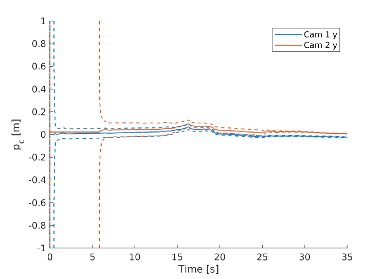
Figure 8: Dual camera y-axis convergence plot with non-overlapping fields of view

V Conclusions

In this paper, we have presented an extension to an EKF-based extrinsic parameter calibration for multiple camera and IMU systems that can be quickly implemented using a variety of existing software for fiducial detection as well as address the issue of time translation when closed loop or hardware synchronization is not possible.

The time translation estimator was tested for both IMU and camera sensors, and showed convergence in both cases. Fast convergence was seen from the sensors using the time translators, which overall reduced the timing noise.

The estimator was tested experimentally with single camera-IMU and dual camera-IMU setups with overlapping fields of view. The estimator converged for all extrinsic calibration parameters in both cases, and the values of one set of parameters was confirmed using a stereo camera calibration tool.

Additionally, experiments were made with non-overlapping fields of view to show the estimator is also capable of converging in these scenarios and is robust against periods without measurement data. The EKF framework showed additional advantages in this type of scenario as cameras not producing measurements still had a reduction in covariance due to the detections of other cameras.

References

- [1] P. Geneva, K. Eckenhoff, W. Lee, Y. Yang, and G. Huang, “OpenVINS: A research platform for visual-inertial estimation,” in Proc. of the IEEE International Conference on Robotics and Automation, Paris, France, 2020.
- [2] J. Delaune, D. S. Bayard, and R. Brockers, “xVIO: A Range-Visual-Inertial Odometry Framework,” oct 2020. [Online]. Available: http://arxiv.org/abs/2010.06677
- [3] P. Furgale, J. Rehder, and R. Siegwart, “Unified temporal and spatial calibration for multi-sensor systems,” in 2013 IEEE/RSJ International Conference on Intelligent Robots and Systems. IEEE, nov 2013, pp. 1280–1286.
- [4] J. Tan, X. An, X. Xu, and H. He, “Automatic extrinsic calibration for an onboard camera,” Proceedings - 2013 Chinese Automation Congress, CAC 2013, no. ii, pp. 340–343, 2013.
- [5] M. Fleps, E. Mair, O. Ruepp, M. Suppa, and D. Burschka, “Optimization based IMU camera calibration,” in 2011 IEEE/RSJ International Conference on Intelligent Robots and Systems. IEEE, sep 2011, pp. 3297–3304.
- [6] F. M. Mirzaei and S. I. Roumeliotis, “A kalman filter-based algorithm for imu-camera calibration,” in 2007 IEEE/RSJ International Conference on Intelligent Robots and Systems, 2007, pp. 2427–2434.
- [7] X. Hu, D. Olesen, and P. Knudsen, “Multistate Constrained Invariant Kalman Filter for Rolling Shutter Camera and Imu Calibration,” Proceedings - International Conference on Image Processing, ICIP, vol. 2020-Octob, pp. 56–60, 2020.
- [8] K. Eckenhoff, P. Geneva, and G. Huang, “MIMC-VINS: A Versatile and Resilient Multi-IMU Multi-Camera Visual-Inertial Navigation System,” IEEE Transactions on Robotics, vol. 37, no. 5, pp. 1360–1380, oct 2021. [Online]. Available: https://ieeexplore.ieee.org/document/9363450/
- [9] N. Parnian and F. Golnaraghi, “Integration of a Multi-Camera Vision System and Strapdown Inertial Navigation System (SDINS) with a Modified Kalman Filter,” Sensors, vol. 10, no. 6, pp. 5378–5394, may 2010. [Online]. Available: http://www.mdpi.com/1424-8220/10/6/5378
- [10] Guodong Chen, Zeyang Xia, Xie Ming, Sun Lining, Junhong Ji, and Zhijiang Du, “Camera calibration based on Extended Kalman Filter using robot’s arm motion,” in 2009 IEEE/ASME International Conference on Advanced Intelligent Mechatronics, no. July. IEEE, jul 2009, pp. 1839–1844.
- [11] J. Hartzer, “multi-cam-imu-cal: Extensible calibration and localization,” 2022. [Online]. Available: https://github.com/unmannedlab/multi-cam-imu-cal
- [12] K. Brink and A. Soloviev, “Filter-based calibration for an imu and multi-camera system,” in Proceedings of the 2012 IEEE/ION Position, Location and Navigation Symposium, 2012, pp. 730–739.
- [13] J. Kelly and G. S. Sukhatme, “Fast relative pose calibration for visual and inertial sensors,” in Experimental Robotics, O. Khatib, V. Kumar, and G. J. Pappas, Eds. Berlin, Heidelberg: Springer Berlin Heidelberg, 2009, pp. 515–524.
- [14] S. Garrido-Jurado, R. Muñoz-Salinas, F. J. Madrid-Cuevas, and M. J. Marín-Jiménez, “Automatic generation and detection of highly reliable fiducial markers under occlusion,” Pattern Recognition, vol. 47, no. 6, pp. 2280–2292, 2014.
- [15] G. Bradski, “The OpenCV Library,” Dr. Dobb’s Journal of Software Tools, 2000.
- [16] S. U. Park and M. J. Chung, “Extrinsic calibration between a 3D laser scanner and a camera using PCA method,” 2012 9th International Conference on Ubiquitous Robots and Ambient Intelligence, URAI 2012, pp. 527–528, 2012.
- [17] O. Kroeger, J. Huegle, and C. A. Niebuhr, “An automatic calibration approach for a multi-camera-robot system,” in 2019 24th IEEE International Conference on Emerging Technologies and Factory Automation (ETFA), vol. 2019-Septe. IEEE, sep 2019, pp. 1515–1518.
- [18] A. English, P. Ross, D. Ball, B. Upcroft, and P. Corke, “TriggerSync: A time synchronisation tool,” in 2015 IEEE International Conference on Robotics and Automation (ICRA), vol. 2015-June, no. June. IEEE, may 2015, pp. 6220–6226.
- [19] H. Sommer, R. Khanna, I. Gilitschenski, Z. Taylor, R. Siegwart, and J. Nieto, “A low-cost system for high-rate, high-accuracy temporal calibration for LIDARs and cameras,” in 2017 IEEE/RSJ International Conference on Intelligent Robots and Systems (IROS), vol. 2017-Septe. IEEE, sep 2017, pp. 2219–2226.
- [20] J. Solà, “Quaternion kinematics for the error-state kalman filter,” October 2015. [Online]. Available: http://arxiv.org/abs/1711.02508
- [21] B.-S. Yaakov, L. X. Rong, and K. Thiagalingam, Estimation with Applications to Tracking and Navigation : Theory Algorithms and Software. Wiley-Interscience, 2001.
- [22] I. The MathWorks, Camera Calibration Toolbox, Natick, Massachusetts, United State, 2021. [Online]. Available: https://www.mathworks.com/help/vision/camera-calibration.html