Revisiting Few-Shot Learning from a Causal Perspective

Abstract

Few-shot learning with $N$-way $K$-shot scheme is an open challenge in machine learning. Many approaches have been proposed to tackle this problem, e.g., the Matching Networks and CLIP-Adapter. Despite that these approaches have shown significant progress, the mechanism of why these methods succeed has not been well explored. In this paper, we interpret these few-shot learning methods via causal mechanism. We show that the existing approaches can be viewed as specific forms of front-door adjustment, which is to remove the effects of confounders. Based on this, we introduce a general causal method for few-shot learning, which considers not only the relationship between examples but also the diversity of representations. Experimental results demonstrate the superiority of our proposed method in few-shot classification on various benchmark datasets. Code is available in the supplementary material.

Introduction

When the available data is rare, few-shot learning (FSL) (Wang et al. 2020) has emerged as an appealing approach and has been widely used on various machine learning tasks (Fan et al. 2021; Liu et al. 2022). In this paper, we focus on $N$-way $K$-shot image classification (Vinyals et al. 2016; Snell, Swersky, and Zemel 2017), where there are $N$ classes and each class has only $K$ labeled training examples.

Many algorithms have been proposed for FSL. For example, metric-based methods (Li et al. 2019) make predictions based on the distance computations between test example and training examples in a learned metric space. Matching Networks (Vinyals et al. 2016) proposed a weighted nearest neighbour classifier given the training data. Prototypical Networks (Snell, Swersky, and Zemel 2017) performed classification by computing distances between test example and class prototypes of training examples. Recently, large-scale pre-trained vision-language models have also shown surprising results for few-shot learning. CLIP-Adapter (Gao et al. 2021) is based on the pre-trained model CLIP (Radford et al. 2021), which is used as a fixed feature extractor, and only fine-tunes the light-weight additional feature adapter for few-shot tasks. Tip-adapter (Zhang et al. 2021) further improves CLIP-Adapter by acquiring the weight of feature adapter from a cache model constructed by training data. Despite the success of these methods, our theoretical understanding of this success remains limited.

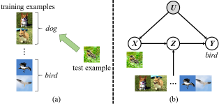
Figure 1: (a) The unobserved confounder such as background would mislead the training model to learn spurious correlation: the model would tend to classify test examples with grass as background as dogs after training. This is incorrect for examples of birds with grass as background. (b) Our proposed causal graph for few-shot learning methods, which are to remove the effects of confounder. $U$: unobserved confounder, $X$: example, $Z$: representation of the example, $Y$: label.

In this paper, we introduce causal mechanism (Glymour, Pearl, and Jewell 2016) to interpret these FSL methods, which provides a unified explanation. In few-shot learning tasks, one of the main challenges is the unobserved confounder (Glymour, Pearl, and Jewell 2016), which causes spurious correlations between the examples and labels. This problem is especially serious in the few-shot setting, since there are only a few training examples which can lead to data bias more easily. As illustrated in Figure 1 (a), the unobserved confounder, such as background “grass”/ “sky”, would mislead the training model to learn spurious correlation, which may lead to the misclassification of examples from a new distribution, e.g., a bird with grass as background. To block the paths from the confounder, back-door adjustment (Glymour, Pearl, and Jewell 2016) and front-door adjustment (Glymour, Pearl, and Jewell 2016) are two popular approaches. In this paper, we revisit the above few-shot learning methods and formalize a causal graph as illustrated in Figure 1 (b). In our proposed causal graph, we interpret the representation of example as the intermediate variable $Z$ between example $X$ and label $Y$. The unobserved confounder $U$ affects the distribution of $X$ and $Y$. We find that existing mainstream FSL methods like Matching Networks and Prototypical Networks can well fit the intervened causal framework in some special cases of the front-door criterion (Glymour, Pearl, and Jewell 2016) (please refer to Section Causal Interpretation for more details).

Based on our causal interpretation, we further propose a general causal method of FSL. We find that previous metric-based methods mainly focus on the way how examples interact while little attention has been paid to the diversity of the representations of examples. Therefore, we propose a general causal few-shot method which considers not only the interaction between examples but also the diversity of representations. In this paper, we propose to use diverse representations from CLIP (Radford et al. 2021) and BLIP (Li et al. 2022). The final prediction is the linear combination of intermediate predictions. Experimental results have shown that our proposed method can make significant improvements on various benchmark datasets. Our method improves 1-shot accuracy from 60.93% to 64.21% and 16-shot accuracy from 65.34% to 72.91% on ImageNet.

The contribution of our work is three-fold:

• We formalize a way of FSL in causal framework. We find that existing mainstream FSL methods can be well explained in the framework.

• We propose a general causal method to deal with FSL problems, which considers both the relationship between examples and the diversity of representations. We also give our method a causal interpretation.

• We evaluate our method on 10 benchmark few-shot image classification datasets and conduct ablation studies to explore its characteristics. Experimental results demonstrate the compelling performance of our method across the board.

Related Work

Metric-Based Few-Shot Learning

Metric-based FSL methods conduct few-shot learning by comparing examples in a learned metric space. Matching Networks (Vinyals et al. 2016) proposed to compare training examples and test examples in a learned metric space. Prototypical Networks (Snell, Swersky, and Zemel 2017) assign test example to the nearest class prototype. CLIP-Adapter (Gao et al. 2021) adopts a simple residual layer as feature adapter over the feature extracted by pre-trained vision-language model CLIP (Radford et al. 2021). Tip-Adapter (Zhang et al. 2021) improves CLIP-Adapter by effectively initializing the weight of feature adapter.

Nevertheless, the success of these methods still lacks a solid theoretical explanation. In this paper, we interpret the success of metric-based methods from the perspective of causal mechanism. Along with the interpretation, we propose a general causal method to deal with few-shot tasks.

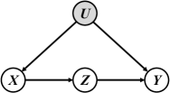
Figure 2: Illustration of front-door adjustment. $U$: unobserved confounder, $X$: example, $Z$: representation of the example, $Y$: label.

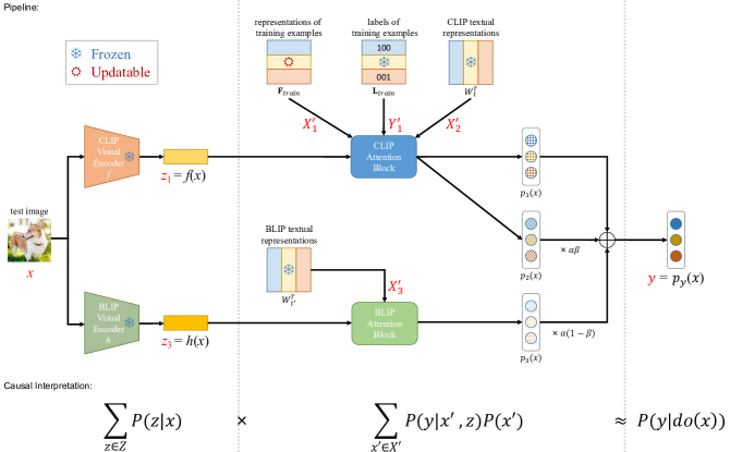
Figure 3: The pipeline of our method and its corresponding causal interpretation in Eq. (3). For a given test example $x$, we first obtain its representations $z_{1}=z_{2}=f(x)$ and $z_{3}=h(x)$ from diverse visual encoders. We then perform intermediate predictions via different Attention Blocks. The final prediction is the linear combination of intermediate predictions. Different parts of the pipeline and their corresponding causal interpretations are separated by dotted lines. Note that we only update representations ${\textbf{F}}_{train}$ as learnable parameters during training.

Causal Inference

Causal inference was recently introduced to machine learning and applied to various tasks, such as image captioning (Yang, Zhang, and Cai 2021), visual grounding (Huang et al. 2021), semantic segmentation (Zhang et al. 2020), representation learning (Mitrovic et al. 2021), and few-shot learning (Yue et al. 2020). A general approach in machine learning is to maximize the observational conditional probability $P(Y|X)$ given example $X$ and label $Y$. However, the existence of confounder (Glymour, Pearl, and Jewell 2016) will mislead the training model to learn spurious correlations between the cause $X$ and the effect $Y$. Causal inference proposes to deconfound (Glymour, Pearl, and Jewell 2016) the training by using a new objective $P(Y|do(X))$ instead of $P(Y|X)$, which aims to find what $X$ truly causes $Y$. The $do$-calculus denotes the pursuit of the causal effect of $X$ on $Y$ by intervening $X=x$. One useful deconfounding causal tool is front-door adjustment (Glymour, Pearl, and Jewell 2016).

Front-Door Adjustment.

Front-door adjustment is a deconfounding way in causal mechanism. Consider the causal graph in Figure 2, where $X$ is example, $Z$ is the representation of $X$, $Y$ is label. $X\rightarrow Z$ represents that $X$ causes $Z$. $U$ is an unobserved confounder that influences both $X$ and $Y$. Confounder $U$ can cause spurious correlation $X\leftarrow U\rightarrow Y$ when the example is irrelevant to the label.

For $x\in X$, $y\in Y$, and $z\in Z$, considering the partial effect of $X$ on $Z$, we have $P(z|do(x))=P(z|x)$ since there is no backdoor path from $X$ to $Z$. On the other side, considering the partial effect of $Z$ on $Y$, we have $P(y|do(z))={\mathbb{E}}_{P(x^{\prime})}P(y|x^{\prime},z)$ for $x^{\prime}\in X$. This is because the backdoor path from $Z$ to $Y$, namely $Z\leftarrow X\leftarrow U\rightarrow Y$, can be blocked by conditioning on $X$. Finally by chaining together the two partial effects $P(z|do(x))$ and $P(y|do(z))$, we have the following front-door adjustment formula:

$$P(y|do(x)) =\sum_{z\in Z}[P(z|do(x))P(y|do(z))]$$

$$=\sum_{z\in Z}[P(z|x){\mathbb{E}}_{P(x^{\prime})}P(y|x^{\prime},z)],$$ (1)

where $P(y|do(x))$ is the true effect of $x$ on $y$.

Pre-trained Vision-Language Models

Pre-trained vision-language models aim to improve the performance of downstream vision and language tasks by pre-training on large amounts of image-text pairs. Pre-trained vision-language models like ALBEF (Li et al. 2021), BLIP (Li et al. 2022), and CLIP (Gao et al. 2021) have shown amazing results on a wide range of downstream tasks even without fine-tuning. They learn the representations of images and texts in the way of contrastive representation learning (Gao et al. 2021), where an image and a text from the same pair are expected to have similar representations.

Causal Interpretation

We consider the traditional $N$-way $K$-shot classification in FSL, where we are asked to perform classification on $N$ classes while we only have access to $K$ training examples from each class.

In this paper, we formalize FSL methods using causal graph as illustrated in Figure 1 (b). Given example $X$, a common procedure in machine learning is to generate its representation $Z$ at first. Then we use the representation $Z$ to make prediction $Y$, i.e., the label of image $X$. $U$ is the unobserved confounder that affects the distribution of example $X$ and label $Y$. We observe that variable $Z$ satisfies the front-door criterion (Glymour, Pearl, and Jewell 2016) between variable $X$ and variable $Y$. For each example $x\in X$, we wish to identify its cause on label $y\in Y$. We adopt the front-door adjustment (Glymour, Pearl, and Jewell 2016) to derive the intervened FSL framework:

$$P(y|do(x))=\sum_{z\in Z}[P(z|x){\mathbb{E}}_{P(x^{\prime})}P(y|x^{\prime},z)],$$ (2)

where probability $P(y|x^{\prime},z)$ can be interpreted as the probability $P(Y=y)$ predicted by exploring the relationship between the representation of $x^{\prime}$ and the representation $z$.

In the following, we will show that the existing few-shot learning methods can be viewed as specific forms of front-door adjustment by setting different values for $P(x^{\prime})$. Let $X^{\prime}$ be a specific value, then we have the following approximation for $x^{\prime}\in X^{\prime}$:

$$P(y|do(x))\approx\sum_{z\in Z}[P(z|x)\sum_{x^{\prime}\in X^{\prime}}P(y|x^{\prime},z)P(x^{\prime})].$$ (3)

Interpretation for Matching Networks

In Matching Networks (MN) (Vinyals et al. 2016), the distance computation is performed for each pair of training example and test example. Let the labeled training set $S=\{(x_{i}^{\prime},y_{i}^{\prime})\}_{i=1}^{NK}$, given a test example $x$, MN computes a probability over $y$ as follows:

$$P_{\rm MN}(y|x,S)=\sum_{i=1}^{NK}a(x,x_{i}^{\prime})y_{i}^{\prime},$$ (4)

where $a$ is an attention mechanism that computes the similarity between two examples. This can be interpreted as a special case in Eq. (3) by letting the representation $z$ of test example $x$ be unique, then the cardinality of representation set $Z$ is exactly one and $P(z|x)=1$. Let $P(y|x^{\prime},z)P(x^{\prime})=a(z,x^{\prime})y^{\prime}$, where $P(x^{\prime})$ is to make sure the summing result is a valid conditional probability, we have:

$$P(y|do(x)) \approx P(z|x)\sum_{x^{\prime}\in X^{\prime}}P(y|x^{\prime},z)P(x^{\prime})$$

$$=1\times\sum_{i=1}^{NK}a(z,x_{i}^{\prime})y_{i}^{\prime}=P_{\rm MN}(y|x,S),$$ (5)

where $X^{\prime}$ is the training set and $a(z,x_{i}^{\prime})=a(x,x_{i}^{\prime})$ since $z$ is the representation of $x$.

According to Eq. (5), we can observe that MN is a method that aims to remove the effects of confounder by considering all examples in the training sets. For example, in Figure 1, if we have more training examples in the training set, e.g., a cat with grass as background, it is possible to remove the effects of confounder since grass is not the distinguishable feature.

Interpretation for Prototypical Networks

In Prototypical Networks(PN) (Snell, Swersky, and Zemel 2017), the representation of test example is also unique and the distance computation is performed between class prototypes of training examples and test example. Let the labeled training set be $S$ and the set of training examples of class $j\in Y$ be $c_{j}$. PN first computes the class prototype $\mu$ as follows:

$$\mu(c_{j})=\frac{1}{|c_{j}|}\sum_{x\in c_{j}}f(x),$$ (6)

where $f(x)$ is the representation of $x$. Given a test example $x$, PN computes probability as follows:

$$P_{\rm PN}(y|x,S) =\sum_{j=1}^{N}a(x,\mu(c_{j}))y_{c_{j}},$$ (7)

where $a$ is an attention mechanism that computes the similarity and $y_{c}$ is the label of examples $c$. This can be interpreted as a special case in Eq. (3):

$$P(y|do(x)) \approx P(z|x)\sum_{c\in C}P(y|c,z)P(c)$$

$$=1\times\sum_{j=1}^{N}a(z,\mu(c_{j}))y_{c_{j}}=P_{\rm PN}(y|x,S),$$ (8)

where $z=f(x)$, $c\in C=\{c_{1},\dots,c_{N}\}$ and $P(y|c,z)P(c)=a(z,\mu(c))y_{c}$.

Interpretation for CLIP/Tip-Adapter

In CLIP-Adapter (Gao et al. 2021), the representation $f(x)$ of an example $x$ is generated by a pre-trained CLIP visual encoder $f$. CLIP-Adapter freezes the CLIP backbone and explore the relationship between the representation $f(x)$ and textual representations $W_{t}$. The logits of CLIP-Adapter(Eq. (2) in  (Zhang et al. 2021)) can be rephrased as follows:

$${\rm logits_{CLIP}}(x)=\tau(f(x))W_{t}^{T},$$ (9)

where $\tau(f(x))$ is the updated representation of example $x$. This can be interpreted as a special case in Eq. (3):

$$P(y|do(x))\approx P(z|x)\sum_{w\in W_{t}}P(y|w,z)P(w),$$ (10)

where $z=\tau(f(x))$ and $\sum_{w\in W_{t}}P(y|w,z)P(w)=zW_{t}^{T}$.

In Tip-Adapter (Zhang et al. 2021), the representation $f(x)$ of an example $x$ is also generated by a pre-trained CLIP visual encoder $f$. Classification is then performed by summing the predictions from two classifiers given the generated representation. The weight of one classifier is derived from visual representations of training set while the weight of another classifier is derived from textual representations of the class names. The logits of Tip-Adapter(Eq. (6) in  (Zhang et al. 2021)) can be rephrased as follows:

$${\rm logits_{TIP}}(x)=\alpha{\rm exp}(-D(x,X^{\prime}))Y^{\prime}+f(x)W_{t}^{T},$$ (11)

where $\alpha>0$ is a hyper-parameter, $D$ is distance function, $Y^{\prime}$ is the one-hot label matrix of training set $X^{\prime}$ and $W_{t}$ is the textual representations. This can be interpreted as a special case in Eq. (3):

$$P(y|do(x))\approx P(z|x)\sum_{x^{\prime}\in X^{\prime}}P(y|x^{\prime},z)P(x^{\prime})$$

$$= P(z|x)[\frac{\alpha}{\alpha+1}\sum_{x^{\prime}\in X^{\prime}}P(y|x^{\prime},z)P(x^{\prime})+$$

$$\frac{1}{\alpha+1}\sum_{x^{\prime}\in X^{\prime}}P(y|x^{\prime},z)P(x^{\prime})]$$

$$= \frac{P(z|x)}{\alpha+1}[\alpha\sum_{x^{\prime}\in X^{\prime}}P(y|x^{\prime},z)P(x^{\prime})+$$

$$\sum_{w\in W_{t}}P(y|w,z)P(w)],$$ (12)

where $z=f(x)$. The same as CLIP-Adapter, Tip-Adapter uses the “class centroid” $w$ in the textual domain provided by the textual encoder given the class name.

Methods aforementioned mainly focus on the relationship between examples, i.e., the term $P(y|x^{\prime},z)$ in Eq. (3) but pay little attention to the diversity of representations, i.e., the term $\sum_{z\in Z}P(z|x)$. Though recent work  (Dvornik, Schmid, and Mairal 2019) has made some effort to improve the diversity of representations, their improvement is limited: 1) They need to fine-tune the whole model, which would lead to over-fitting on some datasets and the training is time-consuming for large-scale vision-language model (Gao et al. 2021; Zhang et al. 2021; Sung, Cho, and Bansal 2022). 2) They use the same backbone for representation learning while we use various backbones for representation learning, which improves the diversity of representations a lot.

Method

Here we propose a general causal method for FSL motivated by Eq. (3). As indicated by Eq. (3), we can design a method considering three aspects: 1) Taking the term $\sum_{z\in Z}P(z|x)$ into consideration, we can obtain diverse representations of example. 2) Taking the term $P(y|x^{\prime},z)$ into consideration, we can make predictions by exploring the relationship between examples such as computing distance in a learned metric space. 3) Taking the term $P(x^{\prime})$ into consideration, the importance of a training example should be relevant to its frequency of occurrence.

The pipeline of our method and its corresponding causal interpretation in Eq. (3) are illustrated in Figure 3. We obtain diverse representations of test example from CLIP (Radford et al. 2021) backbone and from BLIP (Li et al. 2022) backbone. Intermediate predictions are performed via CLIP Attention Block and BLIP Attention Block. The final prediction is the linear combination of intermediate predictions.

CLIP Attention Block.

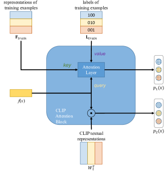
Figure 4: Illustration of CLIP Attention Block. $\odot$ is dot product.

We first consider the representations generated by CLIP backbone. CLIP backbone consists of two parts: visual encoder and textual encoder. For a test example $x$, we first get its L2-normalized $D$-dimension visual representation $f(x)\in{\mathbb{R}}^{1\times D}$ from CLIP visual encoder $f$:

$$f(x)={\rm CLIPVisualEncoder}(x).$$ (13)

Then, for all $NK$ training examples ${\textbf{I}}_{train}$, we obtain their L2-normalized $D$-dimension representations ${\textbf{F}}_{train}\in{\mathbb{R}}^{NK\times D}$ also by using CLIP visual encoder $f$ :

$${\textbf{F}}_{train}=f({\textbf{I}}_{train}).$$ (14)

We get the one-hot labels of training examples ${\textbf{I}}_{train}$, which are denoted as ${\textbf{L}}_{train}\in\{0,1\}^{NK\times N}$.

We now treat representation $f(x)$ as query, representations ${\textbf{F}}_{train}$ as keys, and one-hot labels ${\textbf{L}}_{train}$ as values. The intermediate prediction $p_{1}(x)\in{\mathbb{R}}^{1\times N}$ is performed by the Attention Layer formulated as follows:

$$p_{1}(x) ={\rm AttentionLayer}(f(x);{\textbf{F}}_{train},\textbf{L}_{train})$$

$$={\rm exp}(-(1-f(x){{\textbf{F}}^{T}_{train}})){{\textbf{L}}_{train}}.$$ (15)

Thanks to that query and keys are L2-normalized, the term $(1-f(x){{\textbf{F}}^{T}_{train}})$ is equivalent to computing the Euclidean distances between the representation $f(x)$ and the representations ${\textbf{F}}_{train}$. The exponential function serves as a non-negative transformation for computed distances.

On the other side, we get the L2-normalized $D$-dimension textual representations $W_{t}\in{\mathbb{R}}^{N\times D}$ for $N$ class names by CLIP textual encoder. The intermediate prediction $p_{2}(x)\in{\mathbb{R}}^{1\times N}$ is calculated as follows:

$$p_{2}(x)=f(x)W_{t}^{T}.$$ (16)

The generation of predictions $p_{1}(x)$ and $p_{2}(x)$ is illustrated in Figure 4. The term $p_{1}(x)$ serves as new knowledge from few-shot tasks while the term $p_{2}(x)$ preserves the prior knowledge from CLIP model.

BLIP Attention Block.

We then consider the representations generated by BLIP backbone. BLIP backbone consists of two parts: visual encoder and textual encoder. For a test example $x$, we first get its L2-normalized $D$-dimension visual representation $h(x)\in{\mathbb{R}}^{1\times D}$ from BLIP visual encoder $h$:

$$h(x)={\rm BLIPVisualEncoder}(x).$$ (17)

We then get the L2-normalized $D$-dimension textual representations $W_{t^{*}}\in{\mathbb{R}}^{N\times D}$ for $N$ class names by BLIP textual encoder. The intermediate prediction $p_{3}(x)\in{\mathbb{R}}^{1\times N}$ is calculated as follows:

$$p_{3}(x)=h(x)W_{t^{*}}^{T}.$$ (18)

Final Prediction.

The final prediction $p_{y}(x)\in{\mathbb{R}}^{1\times N}$ is the linear combination of intermediate predictions mentioned above:

$$p_{y}(x)=p_{1}(x)+\alpha[\beta p_{2}(x)+(1-\beta)p_{3}(x)],$$ (19)

where $\alpha$ and $\beta$ are hyper-parameters. Here $\alpha$ controls the trade-off between new knowledge from few-shot tasks and prior knowledge from pre-trained model while $\beta$ controls the trade-off between representations from CLIP backbone and BLIP backbone.

During fine-tuning, we only update representations ${\textbf{F}}_{train}$ as learnable parameters with few-shot training data using cross-entropy loss while other parameters remain fixed. We don’t fine-tune the whole model since fine-tuning large-scale vision-language model would lead to severe over-fitting (Gao et al. 2021; Zhang et al. 2021; Sung, Cho, and Bansal 2022). Besides, the one-hot labels serving as ground-truth annotations should be kept frozen for anti-forgetting. Owing to the good initialization of Attention Layer, our method can adapt to new tasks after a few epochs of updates on training set.

Causal Interpretation

As indicated by Eq. (3), our method considers not only the relationship between examples but also the diversity of representations. We can rephrase our method as follows:

$$P(y|x)= \sum_{z\in Z}[P(z|x)\sum_{x^{\prime}\in X^{\prime}}P(y|x^{\prime},z)P(x^{\prime})]$$

$$= P(z_{1}|x)\sum_{x^{\prime}\in X^{\prime}}P(y|x^{\prime},z_{1})P(x^{\prime})+$$

$$P(z_{2}|x)\sum_{w\in W_{t}}P(y|w,z_{2})P(w)+$$

$$P(z_{3}|x)\sum_{w_{*}\in W_{t^{*}}}P(y|w_{*},z_{3})P(w_{*}),$$ (20)

where $z_{1}$ and $z_{2}$ are both the representation $f(x)$ obtained from CLIP visual encoder, $z_{3}$ is the representation $h(x)$ obtained from BLIP visual encoder, $w$ is the “class centroid” in textual domain provided by CLIP textual encoder and $w_{*}$ is the “class centroid” in textual domain provided by BLIP textual encoder.

Experimental Results

In this section, we evaluate our method w.r.t. classification accuracy on various datasets compared with several state-of-the-art baselines including Zero-shot BLIP (Li et al. 2022), Zero-shot CLIP (Gao et al. 2021), Tip-Adapter (Zhang et al. 2021), and Tip-Adapter-F (Zhang et al. 2021). Besides, we also conduct ablation studies to explore the characteristics of our method.

Datasets and Implementation Detail

We conduct experiments on 10 benchmark image classification datasets: ImageNet (Deng et al. 2009), Caltech101 (Fei-Fei, Fergus, and Perona 2004), DTD (Cimpoi et al. 2014), EuroSAT (Helber et al. 2019), FGVCAircraft (Maji et al. 2013), Flowers102 (Nilsback and Zisserman 2008), Food101 (Bossard, Guillaumin, and Gool 2014), OxfordIIIPet (Parkhi et al. 2012), StanfordCars (Krause et al. 2013), and SUN397 (Xiao et al. 2010). For each dataset, we sample images to construct two disjoint sets: training set and test set. Each method is trained on training set and tested on test set.

For the pre-trained CLIP backbone, we use ResNet-50 (He et al. 2016) as the visual encoder and transformer (Vaswani et al. 2017) as the textual encoder. For the pre-trained BLIP backbone, we use ViT-Large (Dosovitskiy et al. 2020) with $16\times 16$ patch size as the visual encoder and BERT (Devlin et al. 2018) as the textual encoder. The prompt design of CLIP backbone and the way of image pre-processing follows  (Zhang et al. 2021).

During fine-tuning, we only update the representations ${\textbf{F}}_{train}$ in Eq. (15). We use AdamW (Loshchilov and Hutter 2018) as optimizer and the learning rate is set to $10^{-3}$. The batch size is set to 256 for the training set. The hyper-parameter $\alpha$ is set to 100 and $\beta$ to 0.6 in Eq. (19) by default. The number of shots, or the size of the training set, is set to 16 as default.

Models	ImageNet	Caltech101	DTD	EuroSAT	FGVCAircraft
Zero-shot BLIP	47.48	89.11	47.18	35.25	5.52
Zero-shot CLIP	60.32	83.96	41.33	23.50	16.20
Tip-Adapter	61.81	85.35	47.02	45.62	20.13
Tip-Adapter-F	65.34	90.89	67.29	78.25	32.76
Ours	72.91	96.14	69.84	82.75	31.14
Models	Flowers102	Food101	OxfordIIIPet	StanfordCars	SUN397
Zero-shot BLIP	57.11	71.81	59.80	71.06	45.57
Zero-shot CLIP	62.99	76.93	83.05	54.37	58.95
Tip-Adapter	68.87	78.08	84.08	60.45	64.11
Tip-Adapter-F	91.42	81.31	88.58	72.86	71.14
Ours	95.34	86.61	91.01	84.52	75.13

Table 1: Accuracy (%) of different models on various datasets. Methods are evaluated with 16 shots.

Comparison on Various Datasets

Table 1 shows the performance of our method on 10 benchmark image classification datasets. The CLIP visual backbone is ResNet-50 and the BLIP visual backbone is ViT-Large with $16\times 16$ patch size for all methods. As Table 1 shows, our method can greatly improve classification accuracies on various datasets, which are increased by at least 2.43% on ImageNet, Caltech 101, DTD, EuroSAT, Flowers102, Food101, OxfordIIIPet, StanfordCars, and SUN397. Accuracy of our method is marginally lower than that of Tip-Adapter-F on FGVCAircraft by 1.62%. We attribute the degraded performance on FGVCAircraft to the lack of generalization of BLIP on FGVCAircraft since Zero-shot BLIP only achieves 5.52% accuracy on FGVCAircraft.

Comparison on ImageNet

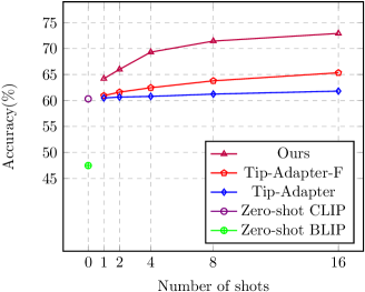
Figure 5: Accuracy(%) of different models with various shots on ImageNet. (Best viewed in color.)

As Figure 5 shows, our method can achieve significant improvement on ImageNet with various shots. Ours surpasses all previous methods in all few-shot settings on ImageNet, which demonstrates the superiority of using diverse representations.

We test our model with various CLIP visual encoders on ImageNet and the number of shots is set to 16. We adopt ResNet (He et al. 2016) and ViT (Dosovitskiy et al. 2020) for comparison. As Table 2 shows, ours can gain significant improvement with various CLIP visual encoders.

Models	RN50	RN101	ViT/32	ViT/16
Zero-shot CLIP	60.32	62.53	63.81	68.74
Tip-Adapter	61.81	64.00	65.31	70.29
Tip-Adapter-F	65.34	68.49	68.62	73.64
Ours	72.91	73.84	73.69	75.82

Table 2: Accuracy (%) of different models with various CLIP visual encoders. RN50 refers to ResNet-50 while ViT/32 refers to ViT-Base with 32 × 32 patch size. Methods are evaluated with 16 shots.

Ablation Studies

In this set of experiments, we conduct ablation studies on ImageNet to analyze the characteristics of our method. All experiments are tested with 16 shots.

Analysis of Different $\alpha$.

As indicated by Eq. (19), hyper-parameter $\alpha$ controls the trade-off between new knowledge from few-shot tasks and prior knowledge from pre-trained model. Therefore, as $\alpha$ becomes smaller, our model tends to learn more from the current few-shot task and less otherwise. $\alpha$ is varied from 1 to 10000 and $\beta$ is set to 0.6. As the top row of Table 3 shows, our model performs best when $\alpha$ is a moderate value 100. This implies that we should strike a good balance between new knowledge from few-shot tasks and prior knowledge from the pre-trained model.

Analysis of Different $\beta$.

As indicated by Eq. (19), hyper-parameter $\beta$ controls the trade-off between representations from CLIP backbone and BLIP backbone. Therefore, as $\beta$ becomes larger, our model tends to depend more on information provided by CLIP backbone and less otherwise. $\beta$ is varied from 0.3 to 0.9 and $\alpha$ is set to 100. As the bottom row of Table 3 shows, our model performs best when $\beta$ is a moderate value 0.6. This implies that the CLIP backbone and BLIP backbone contribute approximately equally to the final prediction.

Analysis of Different Intermediate Predictions.

We further study the effect of each intermediate prediction on the final prediction w.r.t. Eq. (19). We use a tick “$\checked$” to indicate that we adopt the intermediate prediction for the final prediction. Here we set $\alpha$ to 100 and $\beta$ to 0.6 if they appear as the coefficient for the final prediction. Note that during fine-tuning we only update the representations ${\textbf{F}}_{train}$ in Eq. (15) if possible. Prediction $p_{1}$ alone is essentially the same as Matching Networks while few parameters can be updated, prediction $p_{2}$ alone represents Zero-shot CLIP, and prediction $p_{3}$ alone represents Zero-shot BLIP. $p_{1}$ with $p_{2}$ represents Tip-Adapter-F under our hyper-parameter setting. $p_{1}$ along with $p_{2}$ and $p_{3}$ represents our proposed method. As Table 4 shows, prediction from diverse representations is always better than that from a single representation, which strongly demonstrates the necessity for considering the diversity of representations.

$\alpha$	1	10	100	1000	10000
Accuracy(%)	55.65	59.62	72.91	70.26	68.58
$\beta$	0.3	0.45	0.6	0.75	0.9
Accuracy(%)	71.38	72.47	72.91	71.93	69.02

Table 3: Ablation studies of our method varying $\alpha$ and $\beta$.

$p_{1}$	$p_{2}$	$p_{3}$	Accuracy(%)
✓			55.21
	✓		60.32
		✓	47.48
✓	✓		64.72
✓		✓	70.50
	✓	✓	63.19
✓	✓	✓	72.91

Table 4: Ablation studies of our method with different intermediate predictions. We use a tick “$\checked$” to indicate that the intermediate prediction is adopted for the final prediction.

Conclusion

In this paper, we interpreted existing mainstream few-shot learning methods from the perspective of causal mechanism. We interpreted these methods using causal graph. Based on the proposed causal graph, we deconfound the training by intervening the example via front-door adjustment. We observed that the intervened causal framework can well explain existing mainstream few-shot learning methods. Motivated by the intervened causal framework, we proposed a general causal method to tackle few-shot tasks considering not only the relationship between examples but also the diversity of representations. Conducted experimental results have demonstrated the superiority of our proposed method. In our future work, we aim to give a better theoretical explanation for more few-shot learning methods.

References

- Bossard, Guillaumin, and Gool (2014) Bossard, L.; Guillaumin, M.; and Gool, L. V. 2014. Food-101–mining discriminative components with random forests. In European conference on computer vision, 446–461. Springer.
- Cimpoi et al. (2014) Cimpoi, M.; Maji, S.; Kokkinos, I.; Mohamed, S.; and Vedaldi, A. 2014. Describing textures in the wild. In Proceedings of the IEEE conference on computer vision and pattern recognition, 3606–3613.
- Deng et al. (2009) Deng, J.; Dong, W.; Socher, R.; Li, L.-J.; Li, K.; and Fei-Fei, L. 2009. Imagenet: A large-scale hierarchical image database. In 2009 IEEE conference on computer vision and pattern recognition, 248–255. Ieee.
- Devlin et al. (2018) Devlin, J.; Chang, M.-W.; Lee, K.; and Toutanova, K. 2018. Bert: Pre-training of deep bidirectional transformers for language understanding. arXiv preprint arXiv:1810.04805.
- Dosovitskiy et al. (2020) Dosovitskiy, A.; Beyer, L.; Kolesnikov, A.; Weissenborn, D.; Zhai, X.; Unterthiner, T.; Dehghani, M.; Minderer, M.; Heigold, G.; Gelly, S.; et al. 2020. An image is worth 16x16 words: Transformers for image recognition at scale. arXiv preprint arXiv:2010.11929.
- Dvornik, Schmid, and Mairal (2019) Dvornik, N.; Schmid, C.; and Mairal, J. 2019. Diversity with cooperation: Ensemble methods for few-shot classification. In Proceedings of the IEEE/CVF international conference on computer vision, 3723–3731.
- Fan et al. (2021) Fan, Z.; Ma, Y.; Li, Z.; and Sun, J. 2021. Generalized few-shot object detection without forgetting. In Proceedings of the IEEE/CVF Conference on Computer Vision and Pattern Recognition, 4527–4536.
- Fei-Fei, Fergus, and Perona (2004) Fei-Fei, L.; Fergus, R.; and Perona, P. 2004. Learning generative visual models from few training examples: An incremental bayesian approach tested on 101 object categories. In 2004 conference on computer vision and pattern recognition workshop, 178–178. IEEE.
- Gao et al. (2021) Gao, P.; Geng, S.; Zhang, R.; Ma, T.; Fang, R.; Zhang, Y.; Li, H.; and Qiao, Y. 2021. Clip-adapter: Better vision-language models with feature adapters. arXiv preprint arXiv:2110.04544.
- Glymour, Pearl, and Jewell (2016) Glymour, M.; Pearl, J.; and Jewell, N. P. 2016. Causal inference in statistics: A primer. John Wiley & Sons.
- He et al. (2016) He, K.; Zhang, X.; Ren, S.; and Sun, J. 2016. Deep residual learning for image recognition. In Proceedings of the IEEE conference on computer vision and pattern recognition, 770–778.
- Helber et al. (2019) Helber, P.; Bischke, B.; Dengel, A.; and Borth, D. 2019. EuroSAT: A Novel Dataset and Deep Learning Benchmark for Land Use and Land Cover Classification. IEEE Journal of Selected Topics in Applied Earth Observations and Remote Sensing, 12(7): 2217–2226.
- Huang et al. (2021) Huang, J.; Qin, Y.; Qi, J.; Sun, Q.; and Zhang, H. 2021. Deconfounded visual grounding. arXiv preprint arXiv:2112.15324.
- Krause et al. (2013) Krause, J.; Stark, M.; Deng, J.; and Fei-Fei, L. 2013. 3D Object Representations for Fine-Grained Categorization. In Proceedings of the IEEE International Conference on Computer Vision (ICCV) Workshops.
- Li et al. (2019) Li, H.; Eigen, D.; Dodge, S.; Zeiler, M.; and Wang, X. 2019. Finding task-relevant features for few-shot learning by category traversal. In Proceedings of the IEEE/CVF conference on computer vision and pattern recognition, 1–10.
- Li et al. (2022) Li, J.; Li, D.; Xiong, C.; and Hoi, S. 2022. Blip: Bootstrapping language-image pre-training for unified vision-language understanding and generation. arXiv preprint arXiv:2201.12086.
- Li et al. (2021) Li, J.; Selvaraju, R.; Gotmare, A.; Joty, S.; Xiong, C.; and Hoi, S. C. H. 2021. Align before fuse: Vision and language representation learning with momentum distillation. Advances in neural information processing systems, 34: 9694–9705.
- Liu et al. (2022) Liu, J.; Bao, Y.; Xie, G.-S.; Xiong, H.; Sonke, J.-J.; and Gavves, E. 2022. Dynamic Prototype Convolution Network for Few-Shot Semantic Segmentation. In Proceedings of the IEEE/CVF Conference on Computer Vision and Pattern Recognition, 11553–11562.
- Loshchilov and Hutter (2018) Loshchilov, I.; and Hutter, F. 2018. Decoupled Weight Decay Regularization. In International Conference on Learning Representations.
- Maji et al. (2013) Maji, S.; Rahtu, E.; Kannala, J.; Blaschko, M.; and Vedaldi, A. 2013. Fine-grained visual classification of aircraft. arXiv preprint arXiv:1306.5151.
- Mitrovic et al. (2021) Mitrovic, J.; McWilliams, B.; Walker, J. C.; Buesing, L. H.; and Blundell, C. 2021. Representation Learning via Invariant Causal Mechanisms. In International Conference on Learning Representations.
- Nilsback and Zisserman (2008) Nilsback, M.-E.; and Zisserman, A. 2008. Automated flower classification over a large number of classes. In 2008 Sixth Indian Conference on Computer Vision, Graphics & Image Processing, 722–729. IEEE.
- Parkhi et al. (2012) Parkhi, O. M.; Vedaldi, A.; Zisserman, A.; and Jawahar, C. V. 2012. Cats and Dogs. In IEEE Conference on Computer Vision and Pattern Recognition.
- Radford et al. (2021) Radford, A.; Kim, J. W.; Hallacy, C.; Ramesh, A.; Goh, G.; Agarwal, S.; Sastry, G.; Askell, A.; Mishkin, P.; Clark, J.; et al. 2021. Learning transferable visual models from natural language supervision. In International Conference on Machine Learning, 8748–8763. PMLR.
- Snell, Swersky, and Zemel (2017) Snell, J.; Swersky, K.; and Zemel, R. 2017. Prototypical networks for few-shot learning. Advances in neural information processing systems, 30.
- Sung, Cho, and Bansal (2022) Sung, Y.-L.; Cho, J.; and Bansal, M. 2022. Vl-adapter: Parameter-efficient transfer learning for vision-and-language tasks. In Proceedings of the IEEE/CVF Conference on Computer Vision and Pattern Recognition, 5227–5237.
- Vaswani et al. (2017) Vaswani, A.; Shazeer, N.; Parmar, N.; Uszkoreit, J.; Jones, L.; Gomez, A. N.; Kaiser, Ł.; and Polosukhin, I. 2017. Attention is all you need. Advances in neural information processing systems, 30.
- Vinyals et al. (2016) Vinyals, O.; Blundell, C.; Lillicrap, T.; Wierstra, D.; et al. 2016. Matching networks for one shot learning. Advances in neural information processing systems, 29.
- Wang et al. (2020) Wang, Y.; Yao, Q.; Kwok, J. T.; and Ni, L. M. 2020. Generalizing from a few examples: A survey on few-shot learning. ACM computing surveys (csur), 53(3): 1–34.
- Xiao et al. (2010) Xiao, J.; Hays, J.; Ehinger, K. A.; Oliva, A.; and Torralba, A. 2010. Sun database: Large-scale scene recognition from abbey to zoo. In 2010 IEEE computer society conference on computer vision and pattern recognition, 3485–3492. IEEE.
- Yang, Zhang, and Cai (2021) Yang, X.; Zhang, H.; and Cai, J. 2021. Deconfounded image captioning: A causal retrospect. IEEE Transactions on Pattern Analysis and Machine Intelligence.
- Yue et al. (2020) Yue, Z.; Zhang, H.; Sun, Q.; and Hua, X.-S. 2020. Interventional few-shot learning. Advances in neural information processing systems, 33: 2734–2746.
- Zhang et al. (2020) Zhang, D.; Zhang, H.; Tang, J.; Hua, X.-S.; and Sun, Q. 2020. Causal intervention for weakly-supervised semantic segmentation. Advances in Neural Information Processing Systems, 33: 655–666.
- Zhang et al. (2021) Zhang, R.; Fang, R.; Gao, P.; Zhang, W.; Li, K.; Dai, J.; Qiao, Y.; and Li, H. 2021. Tip-adapter: Training-free clip-adapter for better vision-language modeling. arXiv preprint arXiv:2111.03930.