Asynchronous and Error-prone Longitudinal Data Analysis via Functional Calibration

Abstract

In many longitudinal settings, time-varying covariates may not be measured at the same time as responses and are often prone to measurement error. Naive last-observation-carried-forward methods incur estimation biases, and existing kernel-based methods suffer from slow convergence rates and large variations. To address these challenges, we propose a new functional calibration approach to efficiently learn longitudinal covariate processes based on sparse functional data with measurement error. Our approach, stemming from functional principal component analysis, calibrates the unobserved synchronized covariate values from the observed asynchronous and error-prone covariate values, and is broadly applicable to asynchronous longitudinal regression with time-invariant or time-varying coefficients. For regression with time-invariant coefficients, our estimator is asymptotically unbiased, root-n consistent, and asymptotically normal; for time-varying coefficient models, our estimator has the optimal varying coefficient model convergence rate with inflated asymptotic variance from the calibration. In both cases, our estimators present asymptotic properties superior to the existing methods. The feasibility and usability of the proposed methods are verified by simulations and an application to the Study of Women’s Health Across the Nation, a large-scale multi-site longitudinal study on women’s health during mid-life.

1 Introduction

In many decade-long longitudinal studies, participants’ heath information is repeatedly measured by diverse instruments, such as blood tests, physical examinations, nutritional evaluations and psychological assessments. These tests and assessments usually follow different schedules, and are not synchronized in time. The resulting data structures create an asynchronous issue where the response variable and covariates are not measured at the same time. For example, in our motivating Study of Women’s Health Across the Nation (SWAN; https://www.swanstudy.org/), a multi-site longitudinal study on women’s health during their mid-life years, a total of 3,302 women were followed from 1996 to 2008 to study their physical, biological, psychological, and social changes that occurred during the menopausal transition. These health-related metrics were grouped into physical, hormone, and cardiovascular measurements. Fig 1(a) shows the measurement times for hormone, physical and cardiovascular measurements for a random sample of SWAN participants. As seen, these measurements were taken following different schedules. During this important transition, of particular interest is the level of the follicle-stimulating hormone (FSH), our response variable. Two important physical and cardiovascular covariates, the body mass index (BMI) and triglycerides (TG), are also repeatedly measured but on different schedules. Another complication as manifested by Fig 1(b), a spaghetti plot for the longitudinal trajectories of these three variables from a randomly selected participant, is that these asynchronized variables also exhibit short term fluctuations, which need to be modeled as measurement error or nugget effect (Carroll et al., 2006).

There has been some literature on analyzing incomplete longitudinal data using missing data techniques such as the inverse probability weighting: Robins et al. (1995) assumed the response and time-varying covariates must be missing or present simultaneously; Cook et al. (2004) assumed that the repeated measurements within a subject are complete before the subject dropout from the study. These methods rely on parametric modeling of the missing data mechanism and are not designed for data that are asynchronous by design.

More recently, Cao et al. (2015) modeled asynchronous longitudinal data under generalized linear models with either time-invariant or time-varying coefficients, by proposing kernel-weighted estimating equation methods to down-weight covariates that are further away in time from the response. These kernel-weighted estimators are consistent and asymptotically normal, but with slow convergence rates. For time-invariant regression models, their estimated regression coefficients converge in a nonparametric kernel regression rate instead of the usual root-$n$ parametric rate; for time-varying coefficient models, their estimator converges in a bivariate nonparametric smoothing rate, which is much slower than classic convergence rate of varying coefficient models in Cai et al. (2000) and sensitive to bandwidth selection, as shown in our simulation studies. Also, none of the existing methods adequately address the measurement error issue arising from the asynchronous variables.

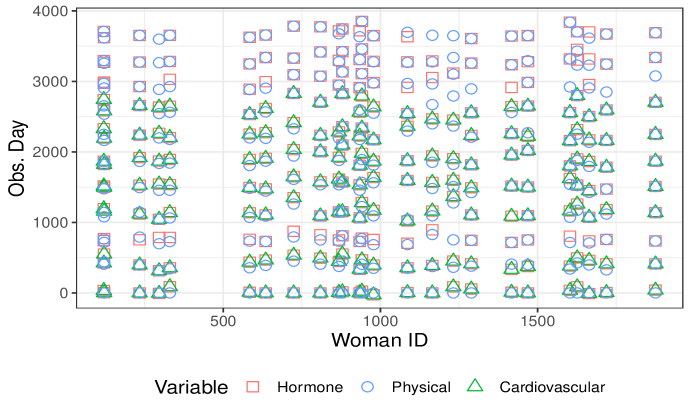
(a)

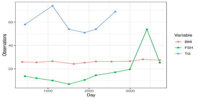
(b)

Figure 1: (a) Observation days for a randomly selected subset of SWAN participants. Each column corresponds to one woman, with points in different colors and shapes representing variables types: hormone, physical and cardiovascular measures. (b) Longitudinal trajectories of follicle-stimulating hormone (FSH), body mass index (BMI), and triglycerides (TG) from a randomly selected SWAN participant (ID = 13959).

To address these limitations, we propose to model the longitudinal trajectories of the covariates in the SWAN study as functional data (Ramsay and Silverman, 2005), and use the functional principal component analysis (FPCA) technique (Li and Hsing, 2010) to impute the missing synchronized covariate values from the observed asynchronous, error-prone covariate values. We then use the imputed values in second stage regression analyses. This method is similar in spirit to the regression calibration method in the measurement error literature (Carroll et al., 2006), but is completely nonparametric. We therefore term our proposed methodology Functional Calibration for Asynchronous Regression (FCAR). The proposed method can be easily implemented using existing software, such as the ‘fdapace’ package in R, and combined with other existing regression methodology such as the common linear regression with time-invariant regression coefficients and the time-varying coefficients (Hoover et al., 1998). We show that our estimators for time-invariant coefficient regression models are root-$n$ consistent and asymptotic normal, while our estimators for time-varying coefficient models enjoy the optimal convergent rate as Hoover et al. (1998), which is one order of magnitude faster than the existing methods such as Cao et al. (2015). We also show that our method can be extended to accommodate multiple asynchronous longitudinal covariate processes using multivariate FPCA (Happ and Greven, 2018; Dai et al., 2021).

We are aware of the related work on asynchronous longitudinal regression using functional data analysis approaches. For example, Şentürk and Müller (2010) and Şentürk et al. (2013) proposed to estimate the time-varying coefficient function by estimating the covariance function of the time-varying covariate and cross-covariance function between the covariate and response processes using bivariate kernel smoothing. However, their method is associated with the same slower bivariate smoothing convergence rate as Cao et al. (2015). Our simulation study shows our method outperforms Şentürk et al. (2013) and Cao et al. (2015) in efficiency and numerical stability.

The paper is organized as follows. We introduce our model assumptions in Section 2, propose the new functional calibration method and apply it to longitudinal regression models with time-invariant or time-varying coefficients in Section 3. The asymptotic properties of the proposed estimators are established in Section 4, while the practical performance of the proposed methods is illustrated by simulation studies in Section 5. We apply the proposed methods to analyze the SWAN data and investigate the potential effects of BMI and triglycerides on follicle-stimulating hormone changes during menopausal transition in Section 6. We provide concluding remarks in Section 7. We present technical proofs and additional numerical results (tables and graphs) and extend the proposed method to multivariate time-varying covariate processes in the Appendix.

2 Model Assumptions

Let $\{X_{i}(t),Y_{i}(t)\}$, $i=1,\ldots,n$, be independent and identically distributed (iid) bivariate longitudinal processes defined on a compact time interval $\mathcal{T}\subset\mathbb{R}$, where $Y_{i}(t)$ is the response of the $i$th subject at time $t$ and $X_{i}(t)$ is the time-varying covariate process. For simplicity, we focus on the case where $X_{i}(t)$ is a univariate process, and present its multivariate extension in Appendix B. We will consider both the time-invariant coefficient model

$$Y_{i}(t)=\beta_{0}+\beta_{1}X_{i}(t)+\epsilon_{i}(t),$$ (1)

and the time-varying coefficient model

$$Y_{i}(t)=\beta_{0}(t)+\beta_{1}(t)X_{i}(t)+\epsilon_{i}(t).$$ (2)

In Model (1), ${\boldsymbol{\beta}}=(\beta_{0},\beta_{1})^{\rm T}$ are the time-invariant intercept and slope parameters, while $\beta_{0}(\cdot)$ and $\beta_{1}(\cdot)$ are the time-varying counterparts in Model (2). In both models, we assume $\epsilon_{i}(t)$ are iid zero-mean error processes with covariance function $\Omega(s,t)={\rm Cov}\{\epsilon(s),\epsilon(t)\}$. We also assume that $X_{i}(t)$ and $\epsilon_{i}(t)$ are independent of each other.

Longitudinal variables are observed on discrete time points. Denote by ${\bf T}_{i}=(T_{i1},\ldots,T_{i{m_{y,i}}})^{\rm T}$ the time points when $Y_{i}(\cdot)$ is observed, and by ${\bf Y}_{i}=(Y_{i1},\ldots,Y_{i{m_{y,i}}})^{\rm T}$ the observed response vector, where $Y_{ij}=Y_{i}(T_{ij})$, $j=1,\ldots,{m_{y,i}}$. On the other hand, in an asynchronous longitudinal design, $X(t)$ are observed on time points ${\bf S}_{i}=(S_{i1},\ldots,S_{i{m_{x,i}}})^{\rm T}$. Let ${\bf X}_{i}=(X_{i1},\ldots,X_{i{m_{x,i}}})^{\rm T}$ where $X_{ij}=X_{i}(S_{ij})$, $j=1,\ldots,{m_{x,i}}$. As illustrated in our motivating example, ${\bf S}_{i}$ and ${m_{x,i}}$ can be completely different from ${\bf T}_{i}$ and ${m_{y,i}}$. In addition, these time-varying covariates are usually contaminated with measurement error (Liao et al., 2011). These measurement errors, not necessarily arising from instrument error, may be due to local variations. In the SWAN study, as the BMI and triglycerides level naturally fluctuate over days or even within the same day, it is reasonable to use their long-term or average values as the “true” values to predict the response; failing to take into account the measurement error can result in biased estimates and reduced statistical power (Carroll et al., 2006). To proceed, we relate $X_{ij}$, the “truth”, to its observed error-contaminated surrogates, $W_{ij}$, via an additive measurement error model:

$$W_{ij}=X_{ij}+U_{ij},\quad j=1,\ldots,{m_{x,i}},\quad i=1,\ldots,n,$$ (3)

where $U_{ij}$ are iid zero-mean measurement errors with variance $\sigma_{u}^{2}$ and independent of ${\bf X}_{i}$. Model (1) or (2), coupled with (3), is referred to as asynchronous longitudinal regression with measurement error.

Let ${\bf W}_{i}=(W_{i1},\ldots,W_{i{m_{x,i}}})^{\rm T}$ be the observed surrogate values that are asynchronous with ${\bf Y}_{i}$, whereas we denote by ${\bf X}_{*i}=\{X_{i}(T_{i1}),\ldots,X_{i}(T_{i{m_{y,i}}})\}^{\rm T}$ the unobserved true covariate values that are synchronized with ${\bf Y}_{i}$. In the measurement error literature (Carroll et al., 2006), a commonly used technique to impute ${\bf X}_{*i}$ from observed surrogate ${\bf W}_{i}$ is regression calibration, which ignores longitudinal correlations, does not capture the dynamic changes in the time-varying covariates and may incur efficiency loss. We instead propose to calibrate the value of ${\bf X}_{*i}$ using a more efficient functional data analysis approach. We assume that the time-varying covariate $X(t),t\in\mathcal{T}$ is a stochastic process defined on $\mathcal{T}$ with mean and covariance functions

$$\mu(t)={\rm E}\{X_{i}(t)\},\quad R(s,t)={\rm Cov}\{X_{i}(s),X_{i}(t)\},\quad s,t,\in\mathcal{T}.$$

The covariance function is a smooth, symmetric, positive semi-definite function with a spectral decomposition of $R(s,t)=\sum_{k=1}^{q}\omega_{k}\psi_{k}(s)\psi_{k}(t)$, where $\omega_{1}\geq\omega_{2}\geq\cdots\geq\omega_{q}>0$ are the eigenvalues, and $\psi_{k}(\cdot)$ are the corresponding eigenfunctions (or principal components) such that $\int_{\cal T}\psi_{k}(t)\psi_{k^{\prime}}(t)dt=I(k=k^{\prime})$. By the Karhunen–Loève theorem,

$$X_{i}(t)=\mu(t)+\hbox{$\sum_{k=1}^{q}$}\xi_{ik}\psi_{k}(t),\quad t\in\mathcal{T},$$ (4)

for $i=1,\ldots,n$, where $\xi_{ik}=\int_{\cal T}\{X_{i}(t)-\mu(t)\}\psi_{k}(t)dt$ are the principal component scores with mean zero and ${\rm Cov}(\xi_{ik},\xi_{ik^{\prime}})=\omega_{k}I(k=k^{\prime})$. The number of principal components $q$ can be infinity in theory, but it is common to assume that $X_{i}(t)$ has a reduced rank representation with a finite $q$ (Li and Hsing, 2010). This is suitable for longitudinal or sparse functional data, where the number of measurements on each trajectories is so small that one cannot realistically estimate a large number of principal components. In practice, $q$ is chosen in a data-driven fashion (Yao et al., 2005; Li et al., 2013), which is to be detailed in Section 3.1.

3 Functional Calibration for Asynchronous Regression

3.1 Calibration using Functional Principal Component Analysis

Let ${\boldsymbol{\mu}}_{i}=\{\mu(S_{i1}),\ldots,\mu(S_{i{m_{x,i}}})\}^{\rm T}$ and ${\boldsymbol{\psi}}_{ik}=\{\psi_{k}(S_{i1}),\ldots,\psi_{k}(S_{i{m_{x,i}}})\}^{\rm T}$, $k=1,\ldots,q$, be the mean and eigenfunctions interpolated on the observed time points, and put ${\bf\Psi}_{i}=[{\boldsymbol{\psi}}_{i1},\ldots,{\boldsymbol{\psi}}_{iq}]$. Under the reduced rank model (4) with a finite rank $q$, the within-subject covariance matrix for ${\bf W}_{i}$ is ${\bf\Sigma}_{i}={\rm Cov}({\bf W}_{i})={\bf\Psi}_{i}{\bf\Lambda}{\bf\Psi}_{i}^{\rm T}+\sigma_{u}^{2}I$, where ${\bf\Lambda}=\hbox{diag}(\omega_{1},\ldots,\omega_{q})$. If ${\boldsymbol{\mu}}_{i}$ and ${\bf\Lambda}$ were known, a roadmap for calibrating the unobserved, synchronized covariates ${\bf X}_{*i}$ would be as follows. First, the best linear unbiased predictors (BLUP) for the FPC scores would be

$$\widetilde{\boldsymbol{\xi}}_{i}=(\widetilde{\xi}_{i1},\ldots,\widetilde{\xi}_{iq})^{\rm T}={\bf\Lambda}{\bf\Psi}_{i}^{\rm T}{\bf\Sigma}_{i}^{-1}({\bf W}_{i}-{\boldsymbol{\mu}}_{i}).$$ (5)

Second, one could predict the functional trajectory of $X_{i}(t)$ by

$$\widetilde{X}_{i}(t)=\mu(t)+\hbox{$\sum_{k=1}^{q}$}\widetilde{\xi}_{ik}\psi_{k}(t).$$ (6)

Finally, interpolating these predicted trajectories on the observation times of $Y$, we could predict the unobserved, synchronized covariates ${\bf X}_{*i}$ by

$$\widetilde{\bf X}_{*i}={\boldsymbol{\mu}}_{*i}+\hbox{$\sum_{k=1}^{q}$}\widetilde{\xi}_{ik}{\boldsymbol{\psi}}_{*ik}={\boldsymbol{\mu}}_{*i}+{\bf\Psi}_{*i}\widetilde{\boldsymbol{\xi}}_{i},$$ (7)

where ${\boldsymbol{\mu}}_{*i}=\{\mu(T_{i1}),\ldots,\mu(T_{i{m_{y,i}}})\}^{\rm T}$, ${\bf\Psi}_{*i}=\{{\boldsymbol{\psi}}_{*i1},\ldots,{\boldsymbol{\psi}}_{*iq}\}$ and ${\boldsymbol{\psi}}_{*ik}=\{\psi_{k}(T_{i1}),\ldots,$ $\psi_{k}(T_{i{m_{y,i}}})\}^{\rm T}$, $k=1,\ldots,q$.

However, as ${\boldsymbol{\mu}}_{i}$ and ${\bf\Lambda}$ are unknown, and in order to complete this calibration roadmap, we need to estimate them based on the observed data $\{{\bf W}_{i},i=1,\ldots,n\}$. Let $K(\cdot)$ be a kernel function, and denote by $K_{h}(u)=K(u/h)/h$ where $h$ is the bandwidth. Following Yao et al. (2005) and Li and Hsing (2010), we use local linear smoothers to estimate mean and covariance functions. For any fixed $t$, we estimate $\mu(t)$ by $\widehat{\mu}(t)=\widehat{a}_{0}$, where

$$(\widehat{a}_{0},\widehat{a}_{1})=\underset{a_{0},a_{1}}{\mathrm{argmin\ }}\dfrac{1}{n}\sum_{i=1}^{n}\dfrac{1}{{m_{x,i}}}\sum_{j=1}^{{m_{x,i}}}\{W_{ij}-a_{0}-a_{1}(S_{ij}-t)\}^{2}K_{h_{\mu}}(S_{ij}-t),$$

with $h_{\mu}>0$ being the bandwidth. We then estimate $R(s,t)$ by $\widehat{R}(s,t)=\widehat{a}_{0}$ with

$$(\widehat{a}_{0},\widehat{a}_{1},\widehat{a}_{2}) = \underset{a_{0},a_{1},a_{2}}{\mathrm{argmin\ }}\dfrac{1}{n}\sum_{i=1}^{n}\bigg{[}\dfrac{1}{M_{x,i}}\sum_{j\neq l}\{L_{ij}L_{il}-a_{0}-a_{1}(S_{ij}-s)-a_{2}(S_{il}-t)\}^{2}$$

$$\hskip 85.35826pt\times K_{h_{R}}(S_{ij}-s)K_{h_{R}}(S_{il}-t)\bigg{]},$$

where $L_{ij}=W_{ij}-\widehat{\mu}(S_{ij})$, $M_{x,i}={m_{x,i}}({m_{x,i}}-1)$, and $h_{R}>0$ is the bandwidth. Similarly, we can estimate the variance function $V(t)={\rm Var}\{W(t)\}=R(t,t)+\sigma_{u}^{2}$ by $\widehat{V}(t)=\widehat{a}_{0}$ where

$$(\widehat{a}_{0},\widehat{a}_{1})=\underset{a_{0},a_{1}}{\mathrm{argmin\ }}\dfrac{1}{n}\sum_{i=1}^{n}\dfrac{1}{{m_{x,i}}}\sum_{j=1}^{{m_{x,i}}}\{L_{ij}^{2}-a_{0}-a_{1}(S_{ij}-t)\}^{2}K_{h_{V}}(S_{ij}-t).$$

Then we estimate $\sigma^{2}_{u}$ by

$$\widehat{\sigma}_{u}^{2}=\dfrac{1}{|\mathcal{T}|}\int_{\mathcal{T}}\{\widehat{V}(t,t)-\widehat{R}(t,t)\}dt.$$

To estimate the functional principal components, we take a spectral decomposition of $\widehat{R}(s,t)$

$$\widehat{R}(s,t)=\hbox{$\sum_{k}$}\widehat{\omega}_{k}\widehat{\psi}_{k}(s)\widehat{\psi}_{k}(t),$$

which can be solved numerically by discretizing the smoothed covariance.

Let $\widehat{\boldsymbol{\mu}}_{i}$, $\widehat{\boldsymbol{\psi}}_{ik}$, $\widehat{\bf\Psi}_{i}$, $\widehat{\bf\Lambda}$, and $\widehat{\bf\Sigma}_{i}$ be the estimated counterparts of ${\boldsymbol{\mu}}_{i}$, ${\boldsymbol{\psi}}_{ik}$, ${\bf\Psi}_{i}$, ${\bf\Lambda}$, and ${\bf\Sigma}_{i}$ using the kernel estimators described above. We adopt the PACE method of Yao et al. (2005) to estimate the principal component score $\xi_{ik}$ by a sample version of BLUP (5), i.e.,

$$\widehat{\boldsymbol{\xi}}_{i}=(\widehat{\xi}_{i1},\ldots,\widehat{\xi}_{iq})^{\rm T}=\widehat{\bf\Lambda}\widehat{\bf\Psi}_{i}^{\rm T}\widehat{\bf\Sigma}_{i}^{-1}\{{\bf W}_{i}-\widehat{\boldsymbol{\mu}}_{i}\}.$$ (8)

With (4), we can recover the covariate process by

$$\widehat{X}_{i}(t)=\widehat{\mu}(t)+\hbox{$\sum_{k=1}^{q}$}\widehat{\xi}_{ik}\widehat{\psi}_{k}(t),\quad t\in\mathcal{T}.$$ (9)

The number of components $q$ can be selected by minimizing the Akaike information criterion (AIC). There are two commonly used versions of AIC based on a marginal log-likelihood (Rice and Wu, 2001),

$$AIC_{marg}(q)=\sum_{i=1}^{n}\left\{m_{i}\log(2\pi)+\log(\det\widehat{\bf\Sigma}_{iq})+({\bf W}_{i}-\widehat{\boldsymbol{\mu}}_{i})^{\rm T}\widehat{\bf\Sigma}_{iq}^{-1}({\bf W}_{i}-\widehat{\boldsymbol{\mu}}_{i})\right\}+2q,$$ (10)

and a conditional log-likelihood (Li et al., 2013),

$$AIC_{cond}(q)=N\log\bigg{(}N^{-1}\sum_{i=1}^{n}||\widehat{\sigma}_{u}^{2}\widehat{\bf\Sigma}_{iq}^{-1}({\bf W}_{i}-\widehat{\boldsymbol{\mu}}_{i})||_{2}^{2}\bigg{)}+N+2nq,$$ (11)

where $N=\sum_{i=1}^{n}{m_{x,i}}$, $\widehat{\bf\Sigma}_{iq}=\widehat{\bf\Psi}_{iq}\widehat{\bf\Lambda}_{q}\widehat{\bf\Psi}_{iq}^{\rm T}+\widehat{\sigma}_{u}^{2}I$, $\widehat{\bf\Lambda}_{q}=\hbox{diag}(\widehat{\omega}_{1},\ldots,\widehat{\omega}_{q})$, $\widehat{\bf\Psi}_{iq}=[\widehat{\boldsymbol{\psi}}_{i1},\ldots,\widehat{\boldsymbol{\psi}}_{iq}]$, and the subscript ‘$q$’ emphasizes the dependence on the number of FPC’s.

3.2 Asynchronous Regression using Calibrated Covariates

With $\widehat{\boldsymbol{\mu}}_{*i}$, $\widehat{\boldsymbol{\psi}}_{*ik}$ and $\widehat{\bf\Psi}_{*i}$ (the kernel estimates interpolated at ${\bf T}_{i}$ instead of ${\bf S}_{i}$), the empirical version of the calibrated covariate $\widetilde{\bf X}_{*i}$ is $\widehat{\bf X}_{*i}=\widehat{\boldsymbol{\mu}}_{*i}+\widehat{\bf\Psi}_{*i}\widehat{\boldsymbol{\xi}}_{i}$, and the design matrices using calibrated covariates are $\mathbb{X}_{i}=({\bf 1},\widehat{\bf X}_{*i})$, $i=1,\ldots,n$. The regression coefficients in Model (1) can be estimated by

$$\widehat{\boldsymbol{\beta}}:=(\widehat{\beta}_{0},\widehat{\beta}_{1})^{\rm T}=({\mathbb{X}}^{\rm T}{\mathbb{X}})^{-1}{\mathbb{X}}^{\rm T}{\bf Y},$$ (12)

where ${\bf Y}=({\bf Y}_{1}^{\rm T},\ldots,{\bf Y}_{n}^{\rm T})^{\rm T}$ and ${\mathbb{X}}=({\mathbb{X}}_{1}^{\rm T},\ldots,{\mathbb{X}}_{n}^{\rm T})^{\rm T}$.

For Model (2), we estimate ${\boldsymbol{\beta}}(t):=\{\beta_{0}(t),\beta_{1}(t)\}^{\rm T}$ by using the local linear estimator of Hoover et al. (1998), with the unobserved $X_{i}(T_{ij})$ replaced by the calibrated value $\widehat{X}_{i}(T_{ij})$ as defined in (9). That is, we estimate ${\boldsymbol{\beta}}(t)$ by $\widehat{\bf b}_{0}$ from

$$(\widehat{\bf b}_{0},\widehat{\bf b}_{1})=\underset{{\bf b}_{0},{\bf b}_{1}}{\mathrm{argmin\ }}\sum_{i=1}^{n}\sum_{j=1}^{{m_{y,i}}}\{Y_{ij}-\mathbb{X}_{ij}^{\rm T}{\bf b}_{0}-\mathbb{X}_{ij}^{\rm T}{\bf b}_{1}(T_{ij}-t)\}^{2}K_{h}(T_{ij}-t),$$ (13)

where ${\mathbb{X}}_{ij}=\{1,\widehat{X}_{i}(T_{ij})\}^{\rm T}$ and $h>0$ is the bandwidth.

4 Asymptotic Theory

4.1 Preliminaries

For ease of exposition, we assume in the asymptotic theory that both $X(t)$ and $Y(t)$ have been centered, such that $\mu(t)\equiv 0$ in (4), $\beta_{0}=0$ in (1) and $\beta_{0}(t)=0$ in (2). We focus on estimating the slope parameter $\beta_{1}$ and the slope function $\beta_{1}(t)$ in Models (1) and (2), respectively; extensions to non-centered situations are straightforward but with more notation. For any positive constant sequences $\{a_{n}\}$ and $\{b_{n}\}$, denote by $a_{n}\prec b_{n}$ if $a_{n}/b_{n}\to 0$ as $n\to\infty$.

Recall ${\bf X}_{*i}$ is the unobserved covariate vector synchronized with the response ${\bf Y}_{i}$, $\widetilde{\bf X}_{*i}={\bf\Psi}_{*i}\widetilde{\boldsymbol{\xi}}_{i}$ is the best linear unbiased predictor of ${\bf X}_{*i}$ as defined in (7), and $\widehat{\bf X}_{*i}$ is the empirical version of $\widetilde{\bf X}_{*i}$ replacing the unknown functions with their kernel estimators. Let ${\boldsymbol{\epsilon}}_{i}=\{\epsilon_{i}(T_{i1}),\ldots,\epsilon_{i}(T_{i{m_{y,i}}})\}^{\rm T}$ be the vector of measurement error as defined in model (1) or (2), with the covariance matrix ${\boldsymbol{\Omega}}_{i}=\{\Omega(T_{ij},T_{ij^{\prime}})\}_{j,j^{\prime}=1}^{{m_{y,i}}}$.

We assume that the numbers of observations $({m_{x,i}},{m_{y,i}})$ are random with $P(2\leq{m_{x,i}},{m_{y,i}}\leq M)=1$ for a constant $M<\infty$. Given ${m_{x,i}}$, $S_{ij}$ are iid copies of the random variable $S$ with a density $f_{S}(\cdot)$; and given ${m_{y,i}}$, $T_{ij}$ are iid copies of the random variable $T$ with a density $f_{T}(\cdot)$. Both $f_{T}(\cdot)$ and $f_{S}(\cdot)$ are strictly greater than 0, with bounded derivatives on ${\cal T}$. Assume that $\{X_{i}(t),\epsilon_{i}(t),{m_{x,i}},{m_{y,i}},{\bf T}_{i},{\bf S}_{i}\}$ are iid tuples across $i$. In addition, we assume the following conditions hold.

1. The kernel function $K(\cdot)$ is a symmetric probability density function on $[-1,1]$ with

   $$\sigma_{K}^{2}:=\int_{-1}^{1}u^{2}K(u)du<\infty,\quad\nu_{0}:=\int_{-1}^{1}K^{2}(u)du<\infty.$$

2. All eigenfunctions $\psi_{k}(t)$, $k=1,\ldots,q$, are twice differentiable, and the second derivatives $\psi_{k}^{{}^{\prime\prime}}(t)$ are uniformly continuous on ${\cal T}$.

3. There exists a constant $C>4$ such that ${\rm E}(|U_{ij}|^{C})+{\rm E}\left\{\underset{t\in\mathcal{T}}{\sup}|X_{i}(t)|^{C}\right\}<\infty$.

4. Assume $h_{R}\to 0$, $h_{V}\rightarrow 0$ as $n\rightarrow\infty$, $(\log n/n)^{1/3}\prec h_{R}\prec n^{-1/4}$ and $(\log n)n^{-3/4}\prec h_{V}\prec n^{-1/4}$.

Remark 1. These conditions are common in functional data analysis. Under them, Li and Hsing (2010) proved that the FPCA estimators possess the following uniform convergence properties

$$\underset{s,t\in\mathcal{T}}{\sup}|\widehat{R}(s,t)-R(s,t)| = O\{h_{R}^{2}+\sqrt{\log n/(nh_{R}^{2})}\}\quad a.s.,$$

$$\widehat{\sigma}_{u}^{2}-\sigma_{u}^{2} = O\{h_{R}^{2}+\sqrt{\log n/(nh_{R})}+h_{V}^{2}+\log n/(nh_{V})\}\quad a.s.,$$

$$\underset{t\in\mathcal{T}}{\sup}|\widehat{\psi}_{k}(t)-\psi_{k}(t)| = O\{h_{R}^{2}+\sqrt{\log n/(nh_{R})}\}\quad a.s.,$$

$$\widehat{\omega}_{k}-\omega_{k} = O(\sqrt{\log n/n})\quad a.s.\quad k=1,\ldots,q.$$

Recall $\widetilde{X}_{i}(t)$ defined in (6) is the BLUP for $X_{i}(t)$ and $\widehat{X}_{i}(t)$ in (9) is its empirical counterpart. By straightforward calculations,

$$\underset{t\in\mathcal{T}}{\sup}|\widehat{X}_{i}(t)-\widetilde{X}_{i}(t)|=O\{h_{R}^{2}+\sqrt{\log n/(nh_{R})}+h_{V}^{2}+\log n/(nh_{V})\}\quad a.s.$$ (14)

It is well-known in the measurement error literature (Carroll et al., 2006), replacing $X_{i}(t)$ with the calibrated value ${\rm E}\{X_{i}(t)\mid{\bf W}_{i}\}$ will result in consistent but less efficient estimators. Equation (14) shows that our functional calibration $\widehat{X}_{i}(t)$ uniformly converges to the BLUP $\widetilde{X}_{i}(t)$, and hence our estimators in (12) and (13) are consistent; however, the derivation of their asymptotic distributions needs much involved analysis.

4.2 Asymptotic Properties of FCAR Estimator for the Time-Invariant Regression Model

The following theorem establishes the asymptotic property of the coefficient estimator (12) under the time-invariant regression model (1).

Theorem 4.1

Under the assumptions above, the estimated slope parameter for model (1) has the following asymptotic distribution

$$\sqrt{n}(\widehat{\beta}_{1}-\beta_{1})\buildrel d\over{\longrightarrow}\hbox{Normal}\{0,(\gamma_{1}+\beta_{1}^{2}\gamma_{2})/\gamma_{x}^{2}\},$$

where

$$\gamma_{x} = {\rm E}(\widetilde{\bf X}_{*i}^{\rm T}\widetilde{\bf X}_{*i})={\rm E}\left\{\mbox{tr}\left({{\bf\Psi}_{*}}_{i}{\bf\Lambda}{\bf\Psi}_{i}^{\rm T}{\bf\Sigma}_{i}^{-1}{\bf\Psi}_{i}{\bf\Lambda}{{\bf\Psi}_{*}}_{i}^{\rm T}\right)\right\},$$

$$\gamma_{1} = {\rm E}\bigg{\{}\mbox{tr}({\bf\Psi}_{*i}{\bf\Lambda}{\bf\Psi}_{i}^{\rm T}{\bf\Sigma}_{i}^{-1}{\bf\Psi}_{i}{\bf\Lambda}{\bf\Psi}_{*i}^{\rm T}{\boldsymbol{\Omega}}_{i})\bigg{\}},$$

$$\gamma_{2} = {\rm Var}\bigg{[}\sum_{j=1}^{m_{y,i}}\widetilde{X}_{i}(T_{ij})\{X_{i}(T_{ij})-\widetilde{X}_{i}(T_{ij})\}+\dfrac{1}{M_{x,i}}\sum_{j\neq j^{\prime}}u^{*}_{i,jj^{\prime}}{\cal A}(S_{ij},S_{ij^{\prime}})\bigg{]},$$ (15)

$u_{i,jj^{\prime}}^{*}=W_{ij}W_{ij^{\prime}}-R(S_{ij},S_{ij^{\prime}})$, ${\cal A}(s_{1},s_{2})$ is defined in Lemma 2 in the Appendix, and the expectations are taken over $({\bf X}_{i},{\boldsymbol{\epsilon}}_{i},{m_{x,i}},{m_{y,i}},{\bf T}_{i},{\bf S}_{i})$.

Remark 2. Under the special case that the BLUP $\widetilde{X}_{i}(t)$ is also the conditional mean ${\rm E}\{X_{i}(t)|{\bf W}_{i}\}$, for example when ${\boldsymbol{\xi}}_{i}$ and ${\bf U}_{i}$ are jointly Gaussian, $\{\widetilde{X}_{i}(t)-X_{i}(t),\ t\in{\cal T}\}$ is uncorrelated with any function of ${\bf W}_{i}$. One can show, under such an circumstance, $\gamma_{2}=\gamma_{21}+\gamma_{22}$, where $\gamma_{21}={\rm Var}[\sum_{j=1}^{m_{y,i}}\widetilde{X}_{i}(T_{ij})\{X_{i}(T_{ij})-\widetilde{X}_{i}(T_{ij})\}]$ and $\gamma_{22}={\rm Var}\{M_{x,i}^{-1}\sum_{j\neq j^{\prime}}u^{*}_{i,jj^{\prime}}{\cal A}(S_{ij},S_{i^{\prime}j^{\prime}})\}$. Under the additional Gaussian assumption on ${\boldsymbol{\xi}}_{i}$ and ${\bf U}_{i}$, we can also obtain

$$\gamma_{21}={\rm E}\left[\mbox{tr}\left\{{{\bf\Psi}_{*}}_{i}{\bf\Lambda}{\bf\Psi}_{i}^{\rm T}{\bf\Sigma}_{i}^{-1}{\bf\Psi}_{i}{\bf\Lambda}{{\bf\Psi}_{*}}_{i}^{\rm T}{{\bf\Psi}_{*}}_{i}{\bf\Lambda}({\bf I}-{\bf\Psi}_{i}^{\rm T}{\bf\Sigma}_{i}^{-1}{\bf\Psi}_{i}{\bf\Lambda}){{\bf\Psi}_{*}}_{i}^{\rm T}\right\}\right].$$

As in the classic regression calibration literature (Carroll et al., 2006), one can define $\widetilde{\boldsymbol{\beta}}$ to be the counterpart of $\widehat{\boldsymbol{\beta}}$ in (12) replacing $\widehat{X}_{i}(t)$ with $\widetilde{X}_{i}(t)$, as if all the functional and scalar parameters in (3) and (4) are known, then $(\gamma_{1}+\beta_{1}^{2}\gamma_{21})/\gamma_{x}^{2}$ is the asymptotic variance of $\widetilde{\beta}_{1}$. In our problem, $\beta_{1}^{2}\gamma_{22}/\gamma_{x}^{2}$ is the additional variation caused by the FPCA estimation errors, i.e. those caused by substituting $\mu(t)$, $\psi_{k}(t)$, $\omega_{k}$ and $\sigma_{u}^{2}$ with their functional estimators described in Section 3.1. .

While it is tempting to treat the calibrated values $\widehat{\bf X}_{*i}$ as the truth and use the naive standard error for linear regression to infer $\beta_{1}$, the decomposition of the asymptotic variance in Theorem 4.1 suggests that this approach ignores the extra variations caused by calibration of the covariate values as well as estimation errors from FPCA. As a result, the naive approach leads to an underestimated variation, a low coverage rate in confidence intervals and illegitimate inferences. We recommend estimating the standard error of $\widehat{\boldsymbol{\beta}}$ using bootstrap, where we resample the subjects and repeat the FPCA procedure to the bootstrap samples to properly account for these extra variations.

4.3 Asymptotic Properties of FCAR Estimator for the Time-Varying Regression Model

Again we assume both $X(t)$ and $Y(t)$ are centered so that $\beta_{0}(t)=0$ and we can focus on estimating $\beta_{1}(t)$ in Model (2). We also make the additional assumptions.

1. The slope function $\beta_{1}(t)$ is twice continuously differentiable on ${\cal T}$.

2. The kernel function in fitting the time-varying regression model in (13) is Lipschitz continuous and satisfies (C.1).

3. The bandwidth $h$ in (13) satisfies $h_{R}/h\to 0$, $\log(n)h^{5}/h_{R}\to 0$, $nh^{7}\to 0$ and $nh\to\infty$.

Theorem 4.2

Under the framework outlined in Section 4.1 and assumptions (C.1)—(C.7), the estimated slope function for model (2) has the following asymptotic distribution

$$\sqrt{nh}\Gamma_{0}(t)\{\widehat{\beta}_{1}(t)-\beta_{1}(t)-\dfrac{1}{2}\beta_{1}^{(2)}(t)\sigma_{K}^{2}h^{2}\}\buildrel d\over{\longrightarrow}\hbox{Normal}[0,\Gamma_{1}(t)+\beta_{1}^{2}(t)\{\Gamma_{2}(t)+\Gamma_{3}(t)\}],$$

for any $t\in\mathcal{T}$, where $\bar{m}_{y}={\rm E}({m_{y,i}})$, $\Gamma_{0}(t)=\bar{m}_{y}f_{T}(t)\Gamma_{x}(t)$,

$$\Gamma_{x}(t) = {\rm Var}\{\widetilde{X}_{i}(t)\}={\boldsymbol{\psi}}^{\rm T}(t){\bf\Lambda}{\rm E}({\bf\Psi}_{i}^{\rm T}{\bf\Sigma}_{i}^{-1}{\bf\Psi}_{i}){\bf\Lambda}{\boldsymbol{\psi}}(t),$$

$$\Gamma_{1}(t) = \bar{m}_{y}\Gamma_{x}(t)\Omega(t,t)f_{T}(t)\nu_{0},$$

$$\Gamma_{2}(t) = \bar{m}_{y}{\rm E}[\widetilde{X}^{2}(t)\{X(t)-\widetilde{X}(t)\}^{2}]\nu_{0},$$

$$\Gamma_{3}(t) = \bar{m}_{y}^{2}f_{S}(t)\nu_{0}\bigg{[}{\rm E}(M_{x,i}^{-1})\int\Pi(t,s_{2},s_{2}){\cal Q}^{2}(s_{2},t)f_{S}(s_{2})ds_{2}$$

$$+{\rm E}\{M_{x,i}^{-1}(m_{x,i}-2)\}\int\Pi(t,s_{2},s_{3}){\cal Q}(s_{2},t){\cal Q}(s_{3},t)f_{S}(s_{2})f_{S}(s_{3})ds_{2}ds_{3}\bigg{]},$$

${\cal Q}(s,t)={\boldsymbol{\psi}}^{\rm T}(t){\bf\Lambda}{\rm E}({\bf\Psi}_{i}^{\rm T}{\bf\Sigma}_{i}^{-1}{\bf\Psi}_{i}){\boldsymbol{\psi}}(s)f_{T}(t)/\{f_{S}(s)f_{S}(t)\}$, $\Pi(s_{1},s_{2},s_{3})={\rm E}\{X^{2}(s_{1})X(s_{2})X(s_{3})\}+R(s_{2},s_{3})\sigma_{u}^{2}-R(s_{1},s_{2})R(s_{1},s_{3})+I(s_{2}=s_{3})\{R(s_{1},s_{1})\sigma_{u}^{2}+\sigma_{u}^{4}\}$, and the expectations are taken over $({m_{x,i}},{m_{y,i}},{\bf T}_{i},{\bf S}_{i},{\bf X}_{i},{\boldsymbol{\epsilon}}_{i})$.

Remark 3. Theorem 4.2 suggests that our estimator enjoys the optimal convergence rate in varying coefficient models as established in Cai et al. (2000), which is much faster than those for the competing method of Cao et al. (2015) and Şentürk and Müller (2010). Analogous to Theorem 4.1, $\Gamma_{0}^{-2}(t)\{\Gamma_{1}(t)+\beta_{1}^{2}(t)\Gamma_{2}(t)\}$ is the asymptotic variance of $\widetilde{\beta}_{1}(t)$, obtained by using $\widetilde{\bf X}_{*i}$ as the predictors in the varying coefficient model (2), and $\Gamma_{0}^{-2}(t)\beta_{1}^{2}(t)\Gamma_{3}(t)$ is the extra variation caused by the FPCA errors. We therefore recommend to make inference on ${\boldsymbol{\beta}}(t)$ using a bootstrap procedure that accounts for the FPCA estimation error as described in Remark 2. Also Assumptions (C.4) and (C.7) require undersmoothing in the FPCA procedure; we need $h_{R}/h\to 0$ so that the biases caused by FPCA estimation are asymptotically negligible compared with the smoothing bias in varying coefficient models.

5 Simulation Studies

We conduct simulations to examine the finite sample performances of the time-invariant regression model (1) and time-varying coefficient model (2), and compare them with those of various exiting methods.

5.1 Simulation 1: FCAR for time-invariant coefficient model

Let the time domain be ${\cal T}=[0,10]$, $X_{i}(t)$ be iid copies of a stochastic process described by model (4) with $q=3$ principal components, and ${\boldsymbol{\xi}}_{i}\sim\hbox{Normal}\{\boldsymbol{0},\hbox{diag}(4,2,1)\}$. Set $n=200$ and generate $Y_{i}(t)$ from Model (1) with $\beta_{0}=1$ and $\beta_{1}=2$. Suppose there are $m=5$ discrete observations on $X_{i}(t)$ and $Y_{i}(t)$, respectively, where $\{S_{i1},\ldots,S_{im}\}$ and $\{T_{i1},\ldots,T_{im}\}$ are generated independently from a uniform distribution on ${\cal T}$. Error-contaminated discrete observations ${\bf W}_{i}$ are generated from Model (3) with $U_{ij}\sim\hbox{Normal}(0,1)$. We consider two settings for the mean and eigenfunctions of $X_{i}(t)$:

Setting I: $\mu(t)=t+\sin(t)$, $\psi_{k}(t)=(1/\sqrt{5})\sin(\pi kt/10)$, $t\in{\cal T}$, $k=1,2,3$;
Setting II: $\mu(t)=\sin(t)$, $\psi_{1}(t)=\sqrt{10}$, $\psi_{2}(t)=\sqrt{5}\sin(2\pi t/10)$, $\psi_{3}(t)=\sqrt{5}\cos(2\pi t/10)$.

We generate residual $\epsilon_{i}(t)$ from a zero-mean Gaussian process with covariance function $\Omega(s,t)={\rm Cov}\{\epsilon_{i}(s),\epsilon_{i}(t)\}$, and consider two different covariance structures: 1) independent (IE) with $\Omega(s,t)=1.5I(s=t)$ and 2) dependent (DE) with $\Omega(s,t)=2^{-|t-s|/5}$. As an ideal case, we also consider a measurement-error free (MEF) scenario under the DE structure, where $X_{ij}$’s in (3) are correctly observed and the covariate measurement error $U_{ij}=0$.

For each setting and each error correlation structure, we simulate 200 data sets and apply the proposed FCAR method to each simulated data set. Specifically, FPCA is performed using the fdapace package of R with its built-in bandwidth selector and $q$ is selected by the marginal likelihood AIC. In Table 1, we summarize the performance of $\widehat{\beta}_{1}$ under both settings and all three measurement error structures (IE, DE and MEF). The criteria include the bias, standard deviation, mean of the naive standard error pretending the calibrated values are the true covariates, coverage rate of a 95% confidence interval using the naive SE, mean of the bootstrap standard error, and coverage rate of a 95% confidence interval using the bootstrap SE. The results on $\widehat{\beta}_{0}$ are similar but less interesting and hence relegated to Appendix C. It appears that the bias of our estimator is much smaller than the standard deviation, corroborating Theorem 4.1 that $\widehat{\beta}_{1}$ is asymptotically unbiased. The results also support Remark 2 that the naive standard error estimator underestimates the standard error and results in confidence intervals with lower than nominal coverage rates. In contrast, bootstrap standard errors capture the extra variations caused by calibrating the covariate value and FPCA estimation errors, and as a result the confidence intervals based on bootstrap standard errors yield coverage rates close to the nominal ones. As noted in Remark 2, we perform FPCA to each bootstrap sample, and Table 1 is based on 500 bootstrap samples.

	Setting I			Setting II
Error type	IE	DE	MEF	IE	DE	MEF
Bias	0.007	0.004	-0.002	-0.008	-0.013	0.025
SD	0.028	0.029	0.017	0.127	0.122	0.060
Naive SE	0.019	0.017	0.012	0.064	0.058	0.034
Naive CP	0.830	0.770	0.820	0.670	0.640	0.725
Bootstrap SE	0.030	0.030	0.019	0.117	0.119	0.064
Bootstrap CP	0.955	0.950	0.965	0.925	0.930	0.940

Table 1: Simulation 1: performance of $\widehat{\beta}_{1}$ under the proposed FCAR method under Settings 1 and 2. SD: standard deviation; Naive SE: mean of the naive standard error; Naive CP: coverage rate of a 95% confidence interval using the naive SE; Bootstrap SE: mean of the bootstrap standard error; Bootstrap CP: coverage rate of a 95% confidence interval using the bootstrap SE; IE: independent errors; DE: dependent errors; MEF: model-error free with dependent errors.

Table 2 compares the proposed FCAR method with the kernel weighted (KW) method (Cao et al., 2015) on biases, Monte Carlo standard deviations, and the average estimated standard errors. For the KW method, we use the function asynchTI from the R package AsynchLong (Cao et al., 2015), which provides a built-in standard error estimator. For FCAR method, the standard error refers to the boostrap standard error in Table 1. It is noteworthy that, under the IE and DE covariance structures, the magnitude of the KW biases still dominates that of the standard errors, yielding confidence intervals with a coverage rate close to 0. In contrast, the proposed FCAR estimator incurs negligible biases and produces confidence intervals with a coverage rate close to the nominal level. The coverage rate of the KW confidence intervals improves much under the ideal MEF (no measurement errors) scenario, but is still lower than that of the FCAR confidence intervals. For the coefficient estimation, FCAR and KW are on par in computational intensity, taking 16.08 and 14.76 seconds respectively; the calculation of standard errors for FCAR takes 1.96 minutes in 10-cores parallel for each data set on average, a bit more than 0.13 seconds taken by KW. This is reasonable, as FCAR needs a bootstrap procedure to compute standard errors, while KW does not. Including an additional setting of $m_{i}=15$ per subject under the DE structure, we investigate the impact of the sparsity level on the performance and find that the performance is fairly robust; see Appendix C.

		IE		DE		MEF
		FCAR	KW	FCAR	KW	FCAR	KW
Setting I	Bias	0.007	-0.225	0.004	-0.213	-0.002	-0.024
	SD	0.028	0.067	0.029	0.067	0.017	0.045
	SE	0.030	0.049	0.030	0.051	0.019	0.032
	CP	0.955	0.060	0.950	0.065	0.965	0.830
Setting II	Bias	-0.008	-0.978	-0.013	-0.978	0.025	-0.060
	SD	0.127	0.097	0.122	0.092	0.060	0.108
	SE	0.117	0.076	0.119	0.077	0.064	0.069
	CP	0.925	0.000	0.930	0.000	0.940	0.735

Table 2: Simulation 1: comparison of $\widehat{\beta}_{1}$ using the proposed FCAR method with the kernel weighted (KW) method of (Cao et al., 2015) on bias, standard deviation (SD), mean of standard error (SE) and coverage rate of a 95% confidence interval using standard error (CP) under two settings and three error structures (IE: independent residuals; DE: dependent residuals; MEF: measurement error free with dependent residuals)

5.2 Simulation 2: FCAR for time-varying coefficient model

We simulate data from the time-varying coefficients regression model (2). As in Simulation 1, we set the time domain to be ${\cal T}=[0,10]$ and simulate $n=200$ subjects with $m_{i}=5$ repeated measures on $X_{i}(t)$ and $Y_{i}(t)$ allowing the measuring time points to be asynchronous between $X$ and $Y$. We simulate $X(t)$ using the Karhunen-Loève expansion (4), with mean function $\mu(t)=t+\sin(t)$, $q=3$, ${\boldsymbol{\xi}}_{i}\sim\hbox{Normal}\{\boldsymbol{0},\hbox{diag}(4,2,1)\}$ and $\psi_{k}(t)=(1/\sqrt{5})\sin(\pi kt/10)$, $k=1,2,3$. We simulate discrete observations $W_{ij}$ from (3) where $U_{ij}$ are iid standard normal, and simulate $Y_{ij}$ from (2), where the measurement error $\epsilon_{i}(t)$ is generated from a mean zero Gaussian process with covariance ${\rm Cov}\{\epsilon_{i}(s),\epsilon_{i}(t)\}=2^{-|t-s|/5}$. For each subject, the observation time points $\{S_{ij}\}$ and $\{T_{ij}\}$ are uniformly distributed on ${\cal T}$ and independent from each other. We consider the following two settings for the time-varying coefficients:

Setting I: $\beta_{0}(t)=0.2t+0.5$, $\beta_{1}(t)=\sin(\pi t/10)$;

Setting II: $\beta_{0}(t)=t^{1/2}$, $\beta_{1}(t)=\sin(\pi t/5)$.

We perform functional calibration using the fdapace package with $AIC$ as the principal component selection criterion. To fit a time-varying coefficients model after the functional calibration, we used the tvLM function in the R package tvReg which implements the kernel smoothing method in Hoover et al. (1998) and its built-in cross-validation procedure to choose the bandwidth. As a comparison, we consider the following estimators, i.e., the Oracle estimator with the known synchronized true values of $X$, the KW estimator (Cao et al., 2015), and the functional varying coefficients model (FVCM) (Şentürk et al., 2013). The Oracle estimator is implemented by using the tvReg package, and the KW method for time-varying coefficient model is implemented by using the authors’s own asynchTD function in the AsynchLong package. The FVCM method requires estimation of the covariance function of $X(t)$ and the cross-covariance function between $X(\cdot)$ and $Y(\cdot)$, which are calculated using the fdapace package. Bandwidths for all methods are selected using the built-in options of the packages mentioned above: generalized cross-validation of fdapace, cross-validation of tvReg and adaptive selection procedure of AsynchLong.

We repeat the simulation 200 times for both settings and apply the proposed and competing methods to each data set. Following Şentürk and Müller (2010), we compare different methods using two evaluation criteria: the mean absolute deviation error (MADE) and the weighted average squared error (WASE)

$$\text{MADE}=\dfrac{1}{2|\mathcal{T}|}\sum_{r=0}^{1}\dfrac{\int_{\mathcal{T}}|\widehat{\beta}_{r}(t)-\beta_{r}(t)|dt}{\text{range}(\beta_{r})},\quad\quad\text{WASE}=\dfrac{1}{2|\mathcal{T}|}\sum_{r=0}^{1}\dfrac{\int_{\mathcal{T}}\{\widehat{\beta}_{r}(t)-\beta_{r}(t)\}^{2}dt}{\text{range}^{2}(\beta_{r})},$$

where $\text{range}(\beta_{r})$ is the range of function $\beta_{r}(t)$, $r=0,1$.

	Method	Criterion	Mean(SD)	Median	25%	75%
Setting I	FCAR	MADE	0.319(0.151)	0.302	0.207	0.388
	FVCM		1.494(2.521)	0.948	0.756	1.418
	KW		1.452(3.533)	1.026	0.868	1.297
	Oracle		0.209(0.091)	0.192	0.142	0.269
	FCAR	WASE	0.345(0.395)	0.224	0.103	0.402
	FVCM		461.495(5235.731)	3.433	1.576	9.553
	KW		1057.299(14234.414)	3.830	1.716	15.221
	Oracle		0.216(0.242)	0.111	0.058	0.294
Setting II	FCAR	MADE	0.263(0.104)	0.246	0.186	0.321
	FVCM		0.944(1.551)	0.616	0.440	0.913
	KW		1.153(1.669)	0.720	0.605	1.115
	Oracle		0.180(0.062)	0.172	0.137	0.220
	FCAR	WASE	0.316(0.351)	0.200	0.093	0.394
	FVCM		299.501(3746.442)	1.464	0.613	5.921
	KW		204.128(1538.798)	2.709	1.196	15.833
	Oracle		0.287(0.347)	0.183	0.088	0.330

Table 3: Simulation 2: MADE and WASE of various methods. SD: standard deviation); 25%: 25% quantile; 75%: 75% quantile.

As summarized in Table 3, the proposed FCAR method yields MADE and WASE that are close to the Oracle estimator. The FVCM and KW methods equipped with built-in tuning parameter selectors perform worse than FCAR, likely because both of them, by evoking bivariate kernel smoothing while estimating univariate coefficient functions in Model (2), are numerically unstable. Both FVCM and KW present large mean WASEs (Fig 2), which are further magnified by the square operator.

MADE and WASE are overall numerical summaries combining $\widehat{\beta}_{0}(\cdot)$ and $\widehat{\beta}_{1}(\cdot)$; we also provide graphical summaries of $\widehat{\beta}_{0}(\cdot)$ and $\widehat{\beta}_{1}(\cdot)$ separately. In Figure 2, we summarize $\widehat{\beta}_{1}(t)$ under Setting I by all 4 methods mentioned above; a similar graph (Figure C.1) under Setting II is provided in the online Appendix. The proposed FCAR estimator for $\beta_{1}(t)$ has negligible biases and overall performance comparable to the Oracle estimator. In contrast, with slower convergence rates and numerical instability of bivariate kernel smoothing, the KW and FVCM estimators for $\beta_{1}(t)$ are highly variable and affected by the boundary effect. Graphical summaries of $\widehat{\beta}_{0}(t)$ allude to the same message. We therefore relegate the graphs on $\widehat{\beta}_{0}(t)$ under these two settings to Figures C.2 and C.3 in Appendix C. Across both settings, FCAR takes an average of 0.45 minutes to estimate the time-varying coefficient functions. A typical run of the bootstrap procedure takes an additional 8.47 minutes under a 10-core parallel. In contrast, KW takes a combined 5.18 minutes for estimation and inference. The FVCM takes an average of 1.93 minutes in estimation, and relies on a bootstrap procedure similar to ours to make inference.

As KW and FVCM are visually sensitive to the boundary effects, we furnish summary tables and plots with the 95% truncated domains in Appendix C for a more fair comparison. In addition, we consider the case of MEF with an added sparsity level of $m_{i}=15$, which again demonstrates the fine performance of the proposed FCAR estimator; see Appendix C.

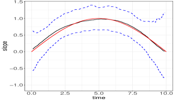
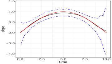
FCAR	Oracle
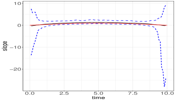
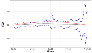
FVCM	KW

Figure 2: Summary of $\widehat{\beta}_{1}(t)$ under Simulation 2, Setting I using various methods. In each panel, black: median of $\widehat{\beta}_{1}(t)$; red: true $\beta_{1}(t)$; dashed blue: 0.975 and 0.025 quantiles.

6 Real Data Analysis

We apply the proposed FCAR method to the SWAN data described in Section 1. The study admitted 3,302 premenopausal or early perimenopausal women between 1996 and 1997, with the baseline age ranging from 42 to 53. These women were scheduled to have annual followups up to 10 years, although various hormonal, physical and cardiovascular biomarkers were measured according different schedules as illustrated in Figure 1 until the study ended in 2008. One of the most important biomarkers in menopausal studies is the follicle-stimulating hormone (FSH) level, the outcome variable of our primary interest.

As declining follicular reserve is the immediate cause of the perimenopausal and menopausal transitions (Richardson et al., 1987), an increase in the serum FSH level was one of the major endocrine changes associated with menopausal transitions (Burger et al., 1995). FSH levels rise progressively before the final menses and will continue for 2–4 years, before remaining elevated postmenopause (Burger et al., 1999). Changes in FSH levels have been linked to or are precursors of various medical conditions. For example, abnormal variations of FSH levels are related to the depressive symptoms during the menopausal transition (Bromberger et al., 2010), and may also increase women’s risk of developing cardiovascular disease after menopause (El Khoudary et al., 2016).

Therefore, studying the dynamic relationship between FSH and other physiological measurements is of great importance to understand women’s reproductive life and their midlife health (Bromberger et al., 2010). Following Wang et al. (2020), we study the association between FSH and triglycerides (TG) adjusting for age, income level and body mass index (BMI). FSH was measured every year for the SWAN participants following the hormone measurement schedule in Figure 1, whereas TG and BMI were following the cardiovascular and physical measurement schedules in Figure 1. Of note, TG was not collected in year 2 or beyond year 8, and 47.5% of BMI measurements were asynchronous with FSH. We also included the baseline age and income as time-invariant covariates, where the income was dichotomized (1 if annual income is more than $50k and 0 otherwise). After removing subjects with missing incomes, there are 1,634 high income subjects and 1,578 low income subjects in the data. We focus our analysis on the first 8 years of the study, when FSH, TG and BMI are all available. An added rationale behind this truncation is that all participants experienced the entire menopausal transition by year 8, becoming postmenopausal or late perimenopausal afterwards (Bromberger et al., 2010).

Existing works, such as Wang et al. (2020), assume the association between FSH and the covariates are time-invariant and ignore asynchronous issue in this data set, which may mask some intriguing time-varying associations. Instead, we apply the time-varying coefficients model to model the dynamic relationship between FSH and other time varying or invariant covariates. Among the competing methods described in Section 5.2, the kernel weighted estimator (KW) requires that all time-varying covariates are measured at the same time points, which is not applicable in our data since TG and BMI are measured on different time as well; the functional varying coefficient model (FVCM) of Şentürk and Müller (2010) was proposed for univariate time-varying covariates and is not readily applicable to multiple time-varying covariates in this data set.

To accommodate two time-varying covariates in our data, we slightly extend the proposed FPCA to a multivariate setting as described in Appendix B and implement it by using the fdapace package in R, where a built-in generalized cross-validation (GCV) procedure is used to select the bandwidths for mean and cross-covariance estimations. We then use the conditional AIC described in (11) to select the number of principal components for TG and BMI separately. To implement the undersmoothing scheme described in condition (C.7), we multiply the GCV selected bandwidths by a factor of $n^{-1/10}$, refit FPCA using the undersmoothing bandwidths, and use the FPCA calibrated values for the subsequent analyses.

We regress FSH against the calibrated TG and BMI values and adjust for time-invariant covariates age and income, using a multivariate time-varying coefficient model

$$Y_{i}(t)=\beta_{0}(t)+{\boldsymbol{\beta}}_{z}^{\rm T}(t){\bf Z}_{i}+{\boldsymbol{\beta}}_{x}^{\rm T}(t){\bf X}_{i}(t)+\epsilon_{i}(t).$$

Fig 3 shows the estimated coefficient functions for TG, BMI, age and income using FCAR, respectively, where the 95% pointwise confidence intervals are obtained using bootstrap. As commented in Remarks 2 and 3, we resample the subjects, perform FPCA using the same bandwidth as in real data to every bootstrap sample in order to properly take into account the FPCA estimation errors. The pointwise confidence intervals in Fig 3 are based on a normal approximation suggested by Theorem 4.2, where the pointwise standard error is estimated based on 200 bootstrap replicates.

The estimated time varying coefficients reveal that FSH is negatively associated with TG, which is consistent with the SWAN data analysis conducted in El Khoudary et al. (2016) using time-invariant regression models. Wang et al. (2020) studied the association between FSH and TG among postmenopausal and perimenopausal women separately using independent studies. The comparison between their results suggests a stronger negative association between FSH and TG among postmenopausal women than perimenopausal women, which supports our findings in Figure 3 (a) that the negative association between FSH and TG becomes stronger through the menopausal transition. Similarly, Figure 3(b) suggests that FSH is negatively associated with BMI. This is consistent with previous findings in the SWAN literature (Randolph Jr et al., 2004), which suggested that the negative association between FSH and BMI becomes stronger throughout the menopausal transition. This time-varying effect of BMI on FSH is not only confirmed by our study, but can be visualized as a continuous curve in Figure 3(b).

Time-invariant variables, such as age and income, are confounders, whose effects need to be adjusted for in the model. The effect of baseline age represents a cohort effect, reflecting different baseline FSH levels in different age cohorts. The positive association between age and FSH seen in Figure 3(c) is consistent with the literature that FSH is elevated as women age through the menopause transition (Burger et al., 1999). Also we find that lower income women are more likely to present higher FSH, agreeing to the literature that links low socioeconomic status to high FSH (Wise et al., 2002), possibly because of poor health awareness (Burger et al., 1995), risk behaviors (Haddad et al., 2008), and inadequate access to health care (Barut et al., 2016).

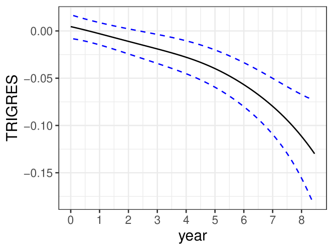
(a) Triglycerides

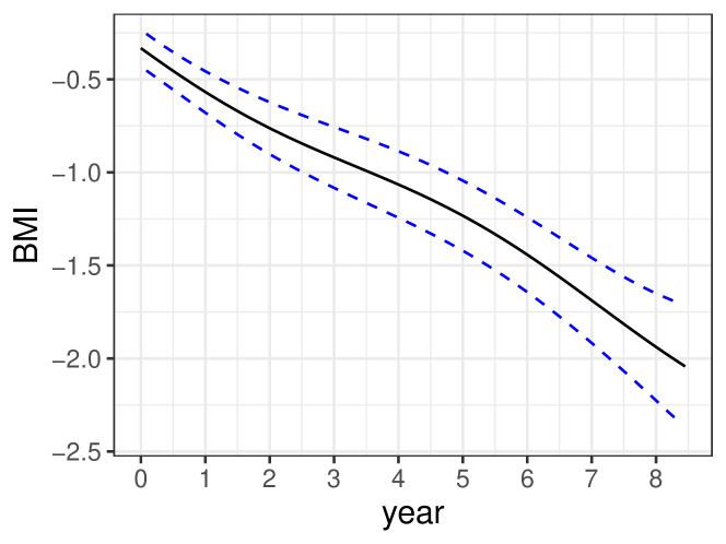
(b) BMI

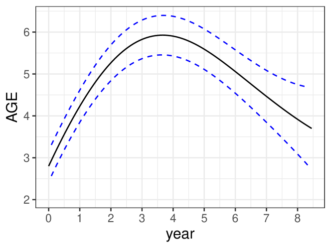
(c) Baseline Age

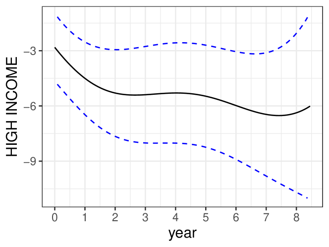
(d) Income

Figure 3: SWAN data analysis using FCAR: time-varying coefficient model on FSH against TG, BMI, age and income. In each panel, the solid curve is the estimated coefficient function and the dashed curves are 95% point-wise confidence intervals obtained using bootstrap.

7 Conclusions

We have proposed a new functional calibration method, termed Functional Calibration for Asynchronous Regression (FCAR), for learning sparse asynchronous longitudinal data. The key idea behind the approach is to calibrate the missing synchronized covariates by the functional principal component analysis (FPCA) approach, which can be easily implemented using existing software. More broadly, our method is applicable to asynchronous longitudinal regression with time-invariant or time-varying coefficients, and addresses a serious limitation of the existing literature. Indeed, our FCAR estimator in a time-invariant regression model enjoys nice asymptotic properties, such as root-$n$ consistency and asymptotic normality. By implementing an undersmoothing scheme in our functional calibration method, the FPCA estimation errors cause a negligible bias to the estimated model, but will inflate the asymptotic variance of the final estimator. Based on these theoretical findings, we recommend to use bootstrap standard error that takes into account FPCA errors, rather than using naive standard errors. Our theoretical analysis as well as our empirical studies show that our proposed method outperforms the existing methods, including the kernel weighted estimator of Cao et al. (2015) and the FVCM method of Şentürk and Müller (2010).

As a reviewer pointed out, the methods of Cao et al. (2015) and Şentürk et al. (2013) can handle generalized outcomes, whereas our investigation has been confined to Gaussian type responses. This extension requires substantial theoretical work and we defer it to future work. As demonstrated in Appendix B and our real data analysis, the proposed FCAR method can be easily implemented for multiple asynchronous time-varying covariates, when the number of time-varying covariates is not too high. When the number is high, the computational load of multivariate FPCA (mFPCA) can rapidly escalate, leading to an unmanageable number of cross-covariance functions to estimate and causing the mFPCA estimators to become unreliable. In these situations, choosing the pertinent time-varying covariates presents a formidable challenge of ‘model selection with error-in-variable,’ as the calibrated covariate values are subject to estimation errors, which are not independent and possess complex structures. These difficulties deserve further exploration.

Supporting Information

Web Appendices A–C, referenced in the main text, are available with this paper at the Biometrics website on Wiley Online Library.

References

- Barut et al. (2016) Barut, M. U., Agacayak, E., Bozkurt, M., Aksu, T., and Gul, T. (2016). There is a positive correlation between socioeconomic status and ovarian reserve in women of reproductive age. Medical science monitor: international medical journal of experimental and clinical research 22, 4386.
- Bromberger et al. (2010) Bromberger, J. T., Schott, L. L., Kravitz, H. M., Sowers, M., Avis, N. E., Gold, E. B., et al. (2010). Longitudinal change in reproductive hormones and depressive symptoms across the menopausal transition: results from the study of women’s health across the nation (swan). Archives of general psychiatry 67, 598–607.
- Burger et al. (1999) Burger, H. G., Dudley, E. C., Hopper, J. L., Groome, N., Guthrie, J. R., Green, A., et al. (1999). Prospectively measured levels of serum follicle-stimulating hormone, estradiol, and the dimeric inhibins during the menopausal transition in a population-based cohort of women. The Journal of Clinical Endocrinology & Metabolism 84, 4025–4030.
- Burger et al. (1995) Burger, H. G., Dudley, E. C., Hopper, J. L., Shelley, J. M., Green, A., Smith, A., et al. (1995). The endocrinology of the menopausal transition: a cross-sectional study of a population-based sample. The Journal of Clinical Endocrinology & Metabolism 80, 3537–3545.
- Cai et al. (2000) Cai, Z., Fan, J., and Li, R. (2000). Efficient estimation and inferences for varying-coefficient models. Journal of the American Statistical Association 95, 888–902.
- Cao et al. (2015) Cao, H., Zeng, D., and Fine, J. P. (2015). Regression analysis of sparse asynchronous longitudinal data. Journal of the Royal Statistical Society, Series B 77, 755–776.
- Carroll et al. (2006) Carroll, R. J., Ruppert, D., Stefanski, L. A., and Crainiceanu, C. M. (2006). Measurement Error in Nonlinear Models: A Modern Perspective. Chapman and Hall/CRC, Boca Raton, FL.
- Cook et al. (2004) Cook, R. J., Zeng, L., and Yi, G. Y. (2004). Marginal analysis of incomplete longitudinal binary data: a cautionary note on locf imputation. Biometrics 60, 820–838.
- Dai et al. (2021) Dai, X., Lin, Z., and Müller, H.-G. (2021). Modeling sparse longitudinal data on riemannian manifolds. Biometrics 77, 1328–1341.
- El Khoudary et al. (2016) El Khoudary, S. R., Santoro, N., Chen, H.-Y., Tepper, P. G., Brooks, M. M., Thurston, R. C., et al. (2016). Trajectories of estradiol and follicle-stimulating hormone over the menopause transition and early markers of atherosclerosis after menopause. European Journal of Preventive Cardiology 23, 694–703.
- Haddad et al. (2008) Haddad, R., Crum, C., Chen, Z., Krane, J., Posner, M., Li, Y., et al. (2008). Hpv16 transmission between a couple with hpv-related head and neck cancer. Oral oncology 44, 812–815.
- Happ and Greven (2018) Happ, C. and Greven, S. (2018). Multivariate functional principal component analysis for data observed on different (dimensional) domains. Journal of the American Statistical Association 113, 649–659.
- Hoover et al. (1998) Hoover, D. R., Rice, J. A., Wu, C. O., and Yang, L.-P. (1998). Nonparametric smoothing estimates of time-varying coefficient models with longitudinal data. Biometrika 85, 809–822.
- Li and Hsing (2010) Li, Y. and Hsing, T. (2010). Uniform convergence rates for nonparametric regression and principal component analysis in functional/longitudinal data. Annals of Statistics 38, 3321–3351.
- Li et al. (2013) Li, Y., Wang, N., and Carroll, R. J. (2013). Selecting the number of principal components in functional data. Journal of the American Statistical Association 108, 1284–1294.
- Liao et al. (2011) Liao, X., Zucker, D. M., Li, Y., and Spiegelman, D. (2011). Survival analysis with error-prone time-varying covariates: A risk set calibration approach. Biometrics 67, 50–58.
- Ramsay and Silverman (2005) Ramsay, J. O. and Silverman, B. W. (2005). Functional Data Analysis. Springer-Verlag,, New York, 2nd edition.
- Randolph Jr et al. (2004) Randolph Jr, J. F., Sowers, M., Bondarenko, I. V., Harlow, S. D., Luborsky, J. L., and Little, R. J. (2004). Change in estradiol and follicle-stimulating hormone across the early menopausal transition: effects of ethnicity and age. The Journal of Clinical Endocrinology & Metabolism 89, 1555–1561.
- Rice and Wu (2001) Rice, J. A. and Wu, C. O. (2001). Nonparametric mixed effects models for unequally sampled noisy curves. Biometrics 57, 253–259.
- Richardson et al. (1987) Richardson, S. J., Senikas, V., and Nelson, J. F. (1987). Follicular depletion during the menopausal transition: evidence for accelerated loss and ultimate exhaustion. The Journal of Clinical Endocrinology & Metabolism 65, 1231–1237.
- Robins et al. (1995) Robins, J. M., Rotnitzky, A., and Zhao, L. P. (1995). Analysis of semiparametric regression models for repeated outcomes in the presence of missing data. Journal of American Statistical Association 90, 106–121.
- Şentürk et al. (2013) Şentürk, D., Dalrymple, L. S., Mohammed, S. M., Kaysen, G. A., and Nguyen, D. V. (2013). Modeling time-varying effects with generalized and unsynchronized longitudinal data. Statistics in Medicine 32, 2971–2987.
- Şentürk and Müller (2010) Şentürk, D. and Müller, H.-G. (2010). Functional varying coefficient models for longitudinal data. Journal of the American Statistical Association 105, 1256–1264.
- Wang et al. (2020) Wang, X., Zhang, H., Chen, Y., Du, Y., Jin, X., and Zhang, Z. (2020). Follicle stimulating hormone, its association with glucose and lipid metabolism during the menopausal transition. Journal of Obstetrics and Gynaecology Research 46, 1419–1424.
- Wise et al. (2002) Wise, L., Krieger, N., Zierler, S., and Harlow, B. (2002). Lifetime socioeconomic position in relation to onset of perimenopause. Journal of Epidemiology & Community Health 56, 851–860.
- Yao et al. (2005) Yao, F., Müller, H.-G., and Wang, J.-L. (2005). Functional data analysis for sparse longitudinal data. Journal of the American Statistical Association 100, 577–590.