FedVeca: Federated Vectorized Averaging on Non-IID Data with Adaptive Bi-directional Global Objective

Abstract

Federated Learning (FL) is a distributed machine learning framework to alleviate the data silos, where decentralized clients collaboratively learn a global model without sharing their private data. However, the clients’ Non-Independent and Identically Distributed (Non-IID) data negatively affect the trained model, and clients with different numbers of local updates may cause significant gaps to the local gradients in each communication round. In this paper, we propose a Federated Vectorized Averaging (FedVeca) method to address the above problem on Non-IID data. Specifically, we set a novel objective for the global model which is related to the local gradients. The local gradient is defined as a bi-directional vector with step size and direction, where the step size is the number of local updates and the direction is divided into positive and negative according to our definition. In FedVeca, the direction is influenced by the step size, thus we average the bi-directional vectors to reduce the effect of different step sizes. Then, we theoretically analyze the relationship between the step sizes and the global objective, and obtain upper bounds on the step sizes per communication round. Based on the upper bounds, we design an algorithm for the server and the client to adaptively adjusts the step sizes that make the objective close to the optimum. Finally, we conduct experiments on different datasets, models and scenarios by building a prototype system, and the experimental results demonstrate the effectiveness and efficiency of the FedVeca method.

I Introduction

Federated learning is a paradigm of distributed machine learning that allows the decentralized clients to train a global model using their own local data, thus alleviating the problems of data silos and user privacy [1, 2]. In FL, the clients’ availability and decentralization bring great communication overhead to the network, and it can be reduced by increasing the local computing [3]. The local computing of FL generally adopts the optimization method of stochastic gradient descent (SGD) [4], which requires the independent and identically distributed (IID) data to ensure the unbiased estimation of the global gradient in the training process [5, 6, 7]. Since the clients’ local data are obtained from the local environment and usage habits, the generated datasets are usually Non-IID due to differences in size and distribution [8]. The Non-IID datasets and multiple local SGD iterations will bring a drift to the global model in each communication round, which significantly reduces the FL performance and stability in the training process, thus requiring more communication rounds to converge or even fail to converge [9, 10, 11]. Therefore, it becomes a key challenge to optimize the FL objective by reducing the negative impact of Non-IID data.

Intuitively, the negative impact is due to the fact that the client has Non-IID data, and the common strategy is to adjust the data distribution from an optimization perspective of the data, thus effectively improving the generalization performance of the global model [12]. Based on this strategy, there is a mean-augmented FL strategy [13] which is inspired by data augmentation methods [14] and allows each client to average the data after exchanging updated model parameters. And the averaged data are sent to each client and used to reduce the degree of local data distribution imbalance. Moreover, other related studies treat each client as a domain, and data augmentation is applied to each client’s data by selecting transformations related to the overall distribution to generate similar data distributions [15, 16]. Rather than modifying data directly, some schemes indirectly improve data distribution through client-side selection. For example, the FL process can be stabilized and sped up by describing the data distribution on the client through the uploaded model parameters, thus the best subsets of clients are intelligently selected in each communication round [17]. Similarly, there is a scheme to evaluate the class distribution without knowing the original data, which uses a client selection strategy oriented towards minimizing class imbalance [18]. And the method proposed in [19] creates a globally shared subset of data to obtain better learning performance in the case of Non-IID data distributions. Besides, there are some schemes that share part of local data to the central server for mitigating the negative impact of Non-IID data [20, 21].

In addition to the optimization of FL strategies by improving data distribution, the broader focus aims at adapting the model to local tasks. For adapting the model, some methods create a better initial model by local fine-tuning. The scheme proposed in [22] makes the local model have a better initial global model by using Model-Agnostic Meta-Learning (MAML) [23]. As an extension, [24] proposes a federated meta-learning formulation using Moreau envelopes. Besides, Multi-tasking is proposed to solve statistical challenges in FL environments by finding relationships between clients’ data such that similar clients learn similar models [25, 26, 27]. With the idea of extracting information from large models to small models, knowledge distillation has also been generalized to optimization strategies for FL [28]. For example, a distillation framework for model fusion with robustness is proposed in [29], using unlabeled data output from client models to train a central classifier that flexibly aggregates heterogeneous models of clients. [30] proposed a domain-adaptive federated optimization method that aligns the learned representations of different clients with the data distribution of the target nodes and uses feature decomposition to enhance knowledge transfer.

The above algorithms are based on the same number of local SGD iterations per client in the training process, and we abbreviate this setup as synchronous FL in the paper. In synchronous FL optimization, the training time always depends on the slowest training node [31]. Besides, some clients are unable to complete the training tasks within the specified time, and these clients will be discarded under normal circumstances, thus affecting the performance and accuracy of the trained model [3]. Since the synchronous FL does not conform to the update principles of clients in real-world environments, it is necessary for each client to have a different number of local SGD iterations. But on Non-IID data, clients with different numbers of local SGD iterations lead to a problem where the global model is biased in the direction of the local model with a higher number of local SGD iterations. To solve this problem, FedProx [32] introduces a regularization term in the local loss function to adjust the distance from the global model, so that there is no need to manually adjust the number of local SGD iterations. Moreover, [33] proposed a local SGD with reduced variance and can further reduce the communication complexity by removing the dependence of different clients on gradient variance, which has a significant performance on Non-IID datasets. Further, SCAFFOLD [34] corrects the direction of global model training by using a control variable (reduction variance), that solves the client-drift problem caused by local SGD iterations on Non-IID datasets. In the FedNova scheme [31], a regularization is introduced based on the contribution of the local gradients, limiting the bias problem for the global model caused by excessive local SGD iterations. However, no current study analyzes the optimal global model and there is no strategy to make the global model close to the optimal global model.

In this paper, we propose a Federated Vectorized Averaging (FedVeca) method to make the global model close to the optimal global model on Non-IID data. Specifically, we define the local gradient as a bi-directional vector with positive and negative. In addition to the direction, we define the step size for the bi-directional vector as the number of local SGD iterations. Then, we adaptively adjust the step size of the averaged bi-directional vector at each client to optimize aggregated global model. The main contributions of this paper are as follows:

• We set a novel objective for the global model of FedVeca. In a qualitative analysis of the relationship between the global objective and the bi-directional vector’s step size, we obtained an upper bound on the step size of each client in each communication round.

• Using the above theoretical upper bound, we propose an algorithm for FedVeca that adaptively balances the step size at each client to accelerate the speed of the global model convergence.

• We evaluate the general performance of the proposed algorithm via extensive experiments on general public datasets, which confirms that the FedVeca algorithm provides efficient performance in the Non-IID datasets.

This paper is organized as follows. The basics and definitions of FL are summarized in Section II. The convergence analysis and control algorithm are presented in Sections III. Experimentation results are shown in Section IV and the conclusion is presented in Section V.

II Preliminaries and Definitions

In this section, we introduce some related preliminaries and our definitions. For convenience, we assume that all vectors are column vectors in this paper and use $\boldsymbol{w}^{T}$ to denote the transpose of $\boldsymbol{w}$. We use “$\triangleq$” to denote “is defined to be equal to” and use $\left\|.\right\|$ to denote the $L$ norm.

II-A Generalized Update Rules of FL

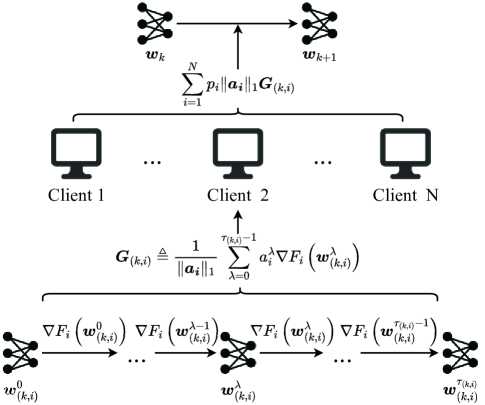
Figure 1: Generalized update rules in the $k$-th round.

Assume that we have $N$ clients with local train datasets $\mathcal{D}_{1},\mathcal{D}_{2},...,\mathcal{D}_{i},...,\mathcal{D}_{N}$, where $i$ denotes the client index. FL performs the training process on these local train datasets under generalized update rules [31]. In the generalized update rules, the training process has $K$ ($K\geq 1$) communication rounds and the server has global model parameters $\boldsymbol{w}_{k}$, where $k=0,1,2,...,K$ denotes the round index. In $k$ round, each client $i$ has $\tau_{(k,i)}$ ($\tau_{(k,i)}\geq 1$) local SGD iterations and its local model parameters $\boldsymbol{w}_{(k,i)}^{\lambda}$, where $\lambda=0,1,2,...,\tau_{(k,i)}$ denotes the local SGD iteration index. When FL begins ($k=0$), the server initializes the global model parameters $\boldsymbol{w}_{0}$ and sends it to all clients. At $\lambda=0$, the local model parameters for all clients are received from the server that $\boldsymbol{w}_{(k,i)}^{0}=\boldsymbol{w}_{k}$. For $0\leq\lambda\leq\tau_{(k,i)}-1$, the gradients $\nabla F_{i}\left(\boldsymbol{w}_{(k,i)}^{\lambda}\right)$ are computed according to the local loss function $F_{i}\left(\boldsymbol{w}\right)$ and the local model parameters $\boldsymbol{w}_{(k,i)}^{\lambda}$, and $\boldsymbol{w}_{(k,i)}^{\lambda}$ are updated by local SGD update rule which is

$$\boldsymbol{w}_{(k,i)}^{\lambda+1}-\boldsymbol{w}_{(k,i)}^{\lambda}=-\eta\nabla F_{i}\left(\boldsymbol{w}_{(k,i)}^{\lambda}\right),$$ (1)

where $\eta>0$ denotes the learning rate which is used in SGD. In this paper, $\eta$ is fixed with a pre-specified value and is equal across all clients.

For each node $i$, the total gradient on the collection of data samples at this node is

$$\boldsymbol{G}_{(k,i)}\triangleq\frac{1}{\|\boldsymbol{a_{i}}\|_{1}}\sum_{\lambda=0}^{\tau_{(k,i)}-1}a_{i}^{\lambda}\nabla F_{i}\left(\boldsymbol{w}_{(k,i)}^{\lambda}\right),$$ (2)

where $\boldsymbol{a}_{i}\in\mathbb{R}^{\tau_{(k,i)}}$ is a non-negative vector and defines how stochastic gradients are locally accumulated, and $a_{i}^{\lambda}$ is the element with index $\lambda$ in the vector $\boldsymbol{a}_{i}$. Under this rule, $\boldsymbol{G}_{(k,i)}$ denotes a locally normalized gradient at node $i$.

After one or multiple local SGD iterations, a global step is performed through the parameter server to update the global model parameters, which is

$$\boldsymbol{w}_{k+1}-\boldsymbol{w}_{k}=-\eta\sum_{i=1}^{N}p_{i}\|\boldsymbol{a_{i}}\|_{1}\boldsymbol{G}_{(k,i)}.$$ (3)

We define $D_{i}\triangleq\left|\mathcal{D}_{i}\right|$ and $D\triangleq\sum_{i=1}^{N}D_{i}$, where $\left|.\right|$ denotes the size of the set, and the weight $p_{i}$ is equal to $D_{i}/D$.

We define that each round $k$ includes one global update step and $\tau_{(k,i)}$ local SGD iterations at each node $i$. In the $k$-th round, the generalized update rules are shown in Fig. 1. Later in this section, we will present two algorithms that are based on these general update rules.

II-B FedAvg and FedNova Algorithms

In the FedAvg and FedNova algorithms, each client performs $E$ epochs (traversals of their local dataset) of local SGD with a mini-batch size $B$. Thus, if a client has $D_{i}$ local data samples, the number of local SGD iterations is $\tau_{(k,i)}=\lfloor E(D_{i}/B)\rfloor$, which can vary widely across clients.

II-B1 The FedAvg Algorithm

The FedAvg algorithm provided the basic principles for FL in the Non-IID datasets. As mentioned in [35], SGD can be seen as an approximation to DGD. Therefore, for convergence analysis of federated optimization, it is generally assumed that the number of local updates is the same across all clients (that is, $\tau_{(k,i)}=\tau$ for all clients i).

According to the definition in Section II-A, FedAvg has $\boldsymbol{a}_{i}=[1,1,...,1]$ and $\|\boldsymbol{a}_{i}\|_{1}=\tau$, the update rule specializes (2) and (3) and is as follows:

$$\left\{\begin{aligned} &\boldsymbol{G}_{(k,i)}\triangleq\sum_{\lambda=0}^{\tau-1}\nabla F_{i}\left(\boldsymbol{w}_{(k,i)}^{\lambda}\right)\\ &\boldsymbol{w}_{k+1}-\boldsymbol{w}_{k}=-\eta\sum_{i=1}^{N}p_{i}\boldsymbol{G}_{(k,i)}.\end{aligned}\right.$$ (4)

Therefore, FedAvg is a simplified special case of the generalized update rules. And next, we will introduce an algorithm that improves on the generalized update rules.

II-B2 The FedNova Algorithm

The FedNova algorithm has the same definition of $\boldsymbol{a}_{i}=[1,1,...,1]$ as the FedAvg algorithm, but FedNova does not impose a special constraint on the number of local SGD iterations, thus $\|\boldsymbol{a_{i}}\|_{1}=\tau_{(k,i)}=\lfloor E(D_{i}/B)\rfloor$. FedNova still uses the local SGD update rule of (1), the locally normalized gradient of (2) and the global aggregation rule is as follows:

$$\left\{\begin{aligned} &\boldsymbol{G}_{(k,i)}\triangleq\frac{1}{\tau_{(k,i)}}\sum_{\lambda=0}^{\tau_{(k,i)}-1}\nabla F_{i}\left(\boldsymbol{w}_{(k,i)}^{\lambda}\right)\\ &\boldsymbol{w}_{k+1}-\boldsymbol{w}_{k}=-\eta\tau_{k}\boldsymbol{d}_{k},\end{aligned}\right.$$ (5)

where $\tau_{k}\triangleq\sum_{i=1}^{N}p_{i}\tau_{(k,i)}$ is the aggregated value of the number of SGD iterations on each client and $\boldsymbol{d}_{k}\triangleq\sum_{i=1}^{N}p_{i}\boldsymbol{G}_{(k,i)}$ is the normalized averaging gradient.

Equation (5) can be seen as a decomposition of equation (3), where $-\boldsymbol{d}_{k}$ denotes the direction of global gradient descent and $\eta\tau_{k}$ denotes the step size of global gradient descent.

II-C Learning Objective and FedVeca Method

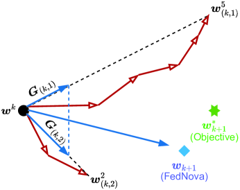
Figure 2: The learning problem in the $k$-th round.

In FL, for each global model $\boldsymbol{w}_{k}$ there is its corresponding loss function $F(\boldsymbol{w}_{k})$. The objective of learning is to find optimal global model $\boldsymbol{w}_{K}^{*}$ to minimize $F(\boldsymbol{w}_{K}^{*})$

$$\boldsymbol{w}_{K}^{*}\triangleq\arg\min F(\boldsymbol{w}_{K}),$$ (6)

thus the value of $F(\boldsymbol{w}_{k})$ should decrease as $k$ increases. In the $k$-th round, we simplify this objective to find an optimal global model $\boldsymbol{w}_{k+1}^{*}$ that is

$$\boldsymbol{w}_{k+1}^{*}\triangleq\arg\min\left\{F(\boldsymbol{w}_{k+1}^{*})-F(\boldsymbol{w}_{k})\right\}.$$ (7)

In FedVeca, we use the update rule (5) of FedNova and define the local gradient $\boldsymbol{G}_{(k,i)}$ as an averaged bi-directional vector whose step size is the value of $\tau_{(k,i)}$. The positive and negative of the bi-directional vector’s direction will be defined in Section III-A. In addition to that, we allow a heterogeneous value of step size at each client and analyze the relationship between our objective $\boldsymbol{w}_{k+1}^{*}$ and FedNova’s global model $\boldsymbol{w}_{k+1}$. As shown in Fig. 2, we assume that there are two clients, one with 5 local SGD iterations (step size of 5) and the other with 2 local SGD iterations (steo size of 2). In order to make the global model $\boldsymbol{w}_{k+1}$ close to our objective $\boldsymbol{w}_{k+1}^{*}$, two factors need to be controlled: direction and step size of the global gradient. According to the definition of $d_{k}$ and $\tau_{k}$ in Section II-B2, we know that the averaged bi-directional vector $\boldsymbol{G}_{(k,i)}$ and it’s step size $\tau_{(k,i)}$ control the direction and step size of the global gradient, respectively. Moreover, we can see in (5) that there is a certain connection between $\boldsymbol{G}_{(k,i)}$ and $\tau_{(k,i)}$, thus a certain connection between the global model $\boldsymbol{w}_{k+1}$ and the bi-directional vector’s step size $\tau_{(k,i)}$.

We set that $\tau_{(k,i)}$ satisfy $\tau_{(k,i)}\neq\lfloor E(D_{i}/B)\rfloor$ and can be different in each round $k$ and at each client $i$. Therefore, a natural question is how to determine the optimal values of $\tau_{(k,i)}$ at each node $i$, so that to get the global objective $\boldsymbol{w}_{k+1}^{*}$. Based on this, if we want to get the optimal $\boldsymbol{w}_{K}^{*}$, we need adaptive control of $\tau_{(k,i)}$ for each round $k$. And next, we will describe how our FedVeca algorithm achieves this objective.

III Convergence Analysis and FedVeca Algorithm

In this section, we first analyze the convergence of FedVeca and get an upper bound of $\tau_{(k,i)}$. Then, we use this upper bound to design our algorithm to adaptively control the value of $\tau_{(k,i)}$ in each round $k$ and at each word node $i$.

III-A Convergence Analysis

We analyze the convergence of FedVeca in this subsection and find an upper bound of $F(\boldsymbol{w}_{k+1})-F(\boldsymbol{w}_{k})$. To facilitate the analysis, we first introduce the definition of the global gradient $\nabla F(\boldsymbol{w}_{k})$ which is the optimal gradient of $\boldsymbol{w}^{*}_{k+1}-\boldsymbol{w}_{k}$ on all training datasets, and we have $\left\|\boldsymbol{d}_{k}\right\|\leq\left\|\nabla F\left(\boldsymbol{w}_{k}\right)\right\|$ by comparing (5) and (7). However, the global gradient $\nabla F(\boldsymbol{w}_{k})$ can not be calculated directly from all training datasets in the $k$-th round of FL. Thus, at the end of each round $k=1,2,...,K$, the server estimate the last global gradient that we define

$$\nabla F(\boldsymbol{w}_{k-1})\triangleq\sum_{i=1}^{N}p_{i}\nabla F_{i}\left(\boldsymbol{w}_{k-1}\right),$$ (8)

where $\nabla F_{i}\left(\boldsymbol{w}_{k-1}\right)$ is the local gradient of $\boldsymbol{w}_{k-1}$ at client $i$ (can be calculated directly from the local training dataset). We assume the global gradient $\nabla F(\boldsymbol{w}_{k-1})$ is convex and all the assumptions in this paper are as follows:

Assumption 1.

Each global gradient is convex and Lipschitz smooth for $k\in[0,k-1]$, that is,

$$\|\nabla F(\boldsymbol{w}_{k+1})-\nabla F(\boldsymbol{w}_{k})\|\leq L\|\boldsymbol{w}_{k+1}-\boldsymbol{w}_{k}\|.$$ (9)

Assumption 2.

For $k\in[0,k-1]$, we have

$$\left\|\boldsymbol{d}_{k}\right\|\leq\left\|\nabla F\left(\boldsymbol{w}_{k}\right)\right\|.$$ (10)

Assumption 3.

For any local gradient $\nabla F_{i}\left(\boldsymbol{w}_{(k,i)}^{\lambda}\right)$ and $\lambda\in[0,\tau_{(k,i)}-1]$, there exist constants $\beta_{(k,i)}\geq 0$ such that

$$\left\|\nabla F_{i}\left(\boldsymbol{w}_{k}\right)-\nabla F_{i}\left(\boldsymbol{w}_{(k,i)}^{\lambda}\right)\right\|\leq\beta_{(k,i)}\left\|\boldsymbol{w}_{k}-\boldsymbol{w}_{(k,i)}^{\lambda}\right\|.$$ (11)

Assumption 4.

For all local gradients, $s\in[0,\lambda]$ and $\lambda\in[1,\tau_{(k,i)}-1]$, there exist constants $\delta_{(k,i)}\geq 0$ such that

$$\left\|\sum_{s=0}^{\lambda-1}\nabla F_{i}\left(\boldsymbol{w}_{(k,i)}^{\lambda}\right)\right\|^{2}\leq\delta_{(k,i)}\sum_{s=0}^{\lambda-1}\left\|\nabla F(\boldsymbol{w}_{k})\right\|^{2}.$$ (12)

Under Assumptions 1 to 4 and the update rule of FedVeca, we get the upper bound of $F(\boldsymbol{w}_{k+1})-F(\boldsymbol{w}_{k})$.

Theorem 1.

In the $k$-th round for $k\in[0,k-1]$, when $\eta\tau_{k}L-1\geq 0$, we have

$$\frac{F\left(\boldsymbol{w}_{k+1}\right)-F\left(\boldsymbol{w}_{k}\right)}{\eta\tau_{k}}$$ (13)

$$\leq\left(\frac{1}{4}\eta\sum_{i=1}^{N}p_{i}\left(\tau_{(k,i)}\left(2L+A_{(k,i)}\right)-A_{(k,i)}\right)-1\right)\left\|\nabla F\left(\boldsymbol{w}_{k}\right)\right\|^{2},$$

where $A_{(k,i)}\triangleq\eta\beta_{(k,i)}^{2}\delta_{(k,i)}$ is a variable that varies with $\delta_{(k,i)}$ and $\beta_{(k,i)}^{2}$.

Proof.

We first perform an inequality transformation on $F\left(\boldsymbol{w}_{k+1}\right)-F\left(\boldsymbol{w}_{k}\right)$ and then convert the equation to contain only the similar items of $\left\|\nabla F\left(\boldsymbol{w}_{k}\right)\right\|^{2}$. For details, see Appendix A ∎

According to Theorem 1, if the model can converge under our method, then it should be consistent with $F\left(\boldsymbol{w}_{k+1}\right)-F\left(\boldsymbol{w}_{k}\right)<0$. It is equivalent to $\frac{1}{4}\eta\sum_{i=1}^{N}p_{i}\left(\tau_{(k,i)}\left(2L+A_{(k,i)}\right)-A_{(k,i)}\right)<1$, and this inequality is related to $\tau_{(k,i)}$. We can see from (13) that the parameters in $A_{(k,i)}$ (the effect of Non-IID) do not play a role when $\tau_{(k,i)}=1$. Therefore, we set the lower bound of $\tau_{(k,i)}>1$, and have another theorem to determine the upper bound on $\tau_{(k,i)}$.

Theorem 2.

In the $k$-th round for $k\in[0,k-1]$, the model converges when

$$\tau_{(k,i)}\leq\frac{A_{(k,i)}}{A_{(k,i)}-\alpha_{k}\min_{i}A_{(k,i)}}$$ (14)

for each client $i$, where $\alpha_{k}$ is a real number and has $\alpha_{k}\in(0,\frac{2L}{\min_{i}A_{(k,i)}})$ (when $\frac{2L}{\min_{i}A_{(k,i)}}<1$) and $\alpha_{k}\in(0,1)$ (when $\frac{2L}{\min_{i}A_{(k,i)}}>1$).

Proof.

For details, see Appendix A ∎

According to (14), we can define the positive and negative direction of the bid-irectional vector (in Section II-C) based on the gap between the value of $A_{(k,i)}$ and the value of $\alpha_{k}\min_{i}A_{(k,i)}$. Further, we can obtain the relationship between the bounds on the step size $\tau_{(k,i)}$ and the corresponding direction of the bi-directional vector. We next describe how our FedVeca algorithm adaptively controls $\tau_{(k,i)}$ to achieve our objective in Section II-C.

III-B FedVeca Algorithm

FL is required to perform more local computations in each communication round [3]. Thus, according to the convex assumption and Theorem 2, we predict that

$$\tau_{(k+1,i)}=\lfloor\frac{A_{(k,i)}}{A_{(k,i)}-\alpha_{k}\min_{i}A_{(k,i)}}\rfloor.$$ (15)

That is, we use the results of the previous round to predict the number of local SGD iterations on each node in the next round. When $\tau_{(k+1,i)}$ is calculated as $\tau_{(k+1,i)}=1$, to keep $\tau_{(k+1,i)}>1$, we reset $\tau_{(k+1,i)}=2$ in our algorithm. Moreover, when $\min_{i}A_{(k,i)}$ is determined in the $k$-th round, we can choose a suitable value of $\alpha_{k}$ to make the global model for the next round close to our global objective (which is mentioned in Section II-C).

As mentioned earlier, the local update runs on the clients and the global aggregation is performed with the assistance of the parameter server. The complete process of the parameter server and each client is presented in Algorithm 1 and Algorithm 2, respectively, where Lines 5-8 of Algorithm 2 are local updates and the rest are considered as part of initialization, global aggregation and computing the value of $\tau_{(k+1,i)}$. We assume that the server initiates the learning process, then initializes $\tau_{(0,i)}$, $\boldsymbol{w}_{0}$ and $\nabla F\left(\boldsymbol{w}_{0}\right)$ and sends it to all clients. The input consists of a given $K$, an $\alpha_{k}$ that transforms with round $k$, and a $\eta$ that is fixed for all rounds, and finally FedVeca algorithm gives the global model $\boldsymbol{w}_{K}$ obtained for the final round $K$.

Algorithm 1 Procedure at the server.

0:  Total round $K$, parameter $\alpha_{k}$ and learning rate $\eta$

0:  $\boldsymbol{w}_{K}$

1:  Initialize $k=0$, $\tau_{(k,i)}$ and $\boldsymbol{w}_{k}$;

2:  repeat

3:     Send $\tau_{(k,i)}$ and $\boldsymbol{w}_{k}$ to all clients;

4:     Receive $\nabla F_{i}(\boldsymbol{w}_{k})$ from each node $i$;

5:     Compute $\nabla F\left(\boldsymbol{w}_{k}\right)$ according to (8) ;

6:     Receive $\boldsymbol{G}_{(k,i)}$ from each node $i$;

7:     Compute $\boldsymbol{w}_{k+1}$ according to (5);

8:     if $k\geq 1$ then

9:        Send $\nabla F\left(\boldsymbol{w}_{k-1}\right)$ to all clients;

10:        Receive $\beta_{(k,i)}$ and $\delta_{(k,i)}$;

11:        if $k=1$ then

12:           Estimate $L_{k-1}\leftarrow\|\nabla F(\boldsymbol{w}_{k-1})\|/\|\boldsymbol{w}_{k-1}\|$;

13:        else

14:           Estimate $L_{k-1}\leftarrow\|\nabla F(\boldsymbol{w}_{k-1})-\nabla F(\boldsymbol{w}_{k-2})\|/$$\|\boldsymbol{w}_{k-1}-\boldsymbol{w}_{k-2}\|$;

15:        end if

16:        Estimate $L\leftarrow\max_{k}L_{k-1}$;

17:        Compute the value of $\tau_{(k+1,i)}$ according to (15);

18:        Compute $\tau_{k+1}$ according to (5);

19:        if $\tau_{(k+1,i)}\leq 1$ then

20:           Set $\tau_{(k+1,i)}=2$;

21:        end if

22:     end if

23:     $k\leftarrow k+1$;

24:     if $k=1$ then

25:        Set $\tau_{(k,i)}=\tau_{(k-1,i)}$;

26:     end if

27:     if $k=K$ then

28:        Set $STOP$ flag, and send it to all clients;

29:     end if

30:  until $STOP$ flag is set

Algorithm 2 Procedure at each client $i$.

1:  Initialize $\lambda\leftarrow 0$, $k=0$ and $\boldsymbol{w}_{(k,i)}^{\lambda}$;

2:  repeat

3:     Receive $\tau_{(k,i)}$ and $\boldsymbol{w}_{k}$ from the server;

4:     Set $\boldsymbol{w}_{(k,i)}^{\lambda}\leftarrow\boldsymbol{w}_{k}$;

5:     for $\lambda=0,1,2,...,\tau_{(k,i)}-1$ do

6:        Compute $\nabla F_{i}\left(\boldsymbol{w}_{(k,i)}^{\lambda}\right)$;

7:        Perform local update of $\boldsymbol{w}_{(k,i)}^{\lambda}$ according to (1);

8:     end for

9:     Compute $F_{i}\left(\boldsymbol{w}_{k}\right)$;

10:     Send $F_{i}\left(\boldsymbol{w}_{k}\right)$ to parameter server;

11:     Compute $\boldsymbol{G}_{(k,i)}$ according to (5);

12:     Send $\boldsymbol{G}_{(k,i)}$ to parameter server;

13:     if $k\geq 1$ then

14:        Receive $\nabla F\left(\boldsymbol{w}_{k-1}\right)$ from the server;

15:        Estimate $\beta_{(k,i)}^{\lambda}\leftarrow\left\|\nabla F_{i}\left(\boldsymbol{w}_{k}\right)-\nabla F_{i}\left(\boldsymbol{w}_{(k,i)}^{\lambda}\right)\right\|/$$\left\|\boldsymbol{w}_{k}-\boldsymbol{w}_{(k,i)}^{\lambda}\right\|$ for $\lambda\in[0,\tau_{(k,i)}-1]$;

16:        Estimate $\beta_{(k,i)}\leftarrow\max_{\lambda}\beta_{(k,i)}^{\lambda}$;

17:        Estimate $\delta_{(k,i)}^{\lambda}\leftarrow\left\|\sum_{s=0}^{\lambda}\nabla F_{i}\left(\boldsymbol{w}_{(k,i)}^{s}\right)\right\|^{2}/$ $\sum_{s=0}^{\lambda}\left\|\nabla F(\boldsymbol{w}_{k-1})\right\|^{2}$ for $\lambda\in[1,\tau_{(k,i)}-1]$;

18:        Estimate $\delta_{(k,i)}\leftarrow\max_{\lambda}\delta_{(k,i)}^{\lambda}$;

19:        Send $\beta_{(k,i)}$ and $\delta_{(k,i)}$ to parameter server;

20:     end if

21:     $k\leftarrow k+1$;

22:  until $STOP$ flag is received

III-B1 Handling of SGD

When using SGD with FedVeca algorithm at all clients, all their gradients are computed on mini-batches. Each SGD step corresponds to a model update step where the gradient is computed on a mini-batch of local training data in Line 6 of Algorithm 2. The mini-batch changes for every step of the local iteration, i.e., for each new local iteration, a new mini-batch of a given size is randomly selected from the local training data. After $\tau_{(k,i)}$ local update steps, we average the corresponding model gradient vectors on these training data and get obtain the direction vector $G_{(k,i)}$ of SGD at node $i$ (Line 11 of Algorithm 2).

When the parameter server receives $G_{(k,i)}$ from each client, it updates $\boldsymbol{w}_{k+1}$ (Line 7 of Algorithm 1) according to the second term in (5) where $\tau_{k}$ is calculated based on $\tau_{(k,i)}$ in Line 18 of Algorithm 1. When the program proceeds to the set number of rounds $k$, the final model parameter $\boldsymbol{w}_{K}$ is obtained at the server in Lines 27-29 of Algorithm 1. Then we set the $STOP$ flag to stop the server-side program and send the flag to all clients to stop the local program.

III-B2 Estimation of Parameters

According to Assumptions 1, 3 and 4, we have three parameters $L$, $\beta_{(k,i)}$ and $\delta_{(k,i)}$ that need to be estimated in real-time during the learning process. $L$ is the parameter describing the smooth of global gradients and should be ensured to satisfy Assumption 1, so we perform the estimation of its maximum value (in all rounds for $k>0$) on the server side in Lines 16 of Algorithm 1. Estimating $L$ requires the global gradient of the previous round, which does not exist when $k=0$, so we give this program a delay of one round in Lines 14 of Algorithm 1. We know that $L$ is not involved in the calculation of the new $\tau_{(k,i)}$ in (15) and used to satisfy that premise $\eta\tau_{k}L-1\geq 0$ of Theorem 1, so a delay of one round in its estimation $L_{k-1}$ has little effect on the final result.

Therefore FedVeca algorithm should estimate the value of $A_{(k,i)}$. The expression of $A_{(k,i)}$ includes parameters $\beta_{(k,i)}$ and $\delta_{(k,i)}$ which need to be estimated in practice on the client side. Before starting the estimation, we need to calculate $F_{i}\left(\boldsymbol{w}_{k}\right)$ on the local training dataset in Line 9 of Algorithm 2. Then, the estimation of $\beta_{(k,i)}$ is computed from $\lambda=0$ to $\lambda=\tau_{(k,i)}-1$ and the estimation of $\delta_{(k,i)}$ is computed from $\lambda=1$ to $\lambda=\tau_{(k,i)}-1$ in Lines 15 and 17 of Algorithm 2. Finally, the largest estimations of $\beta_{(k,i)}$ and $\delta_{(k,i)}$ from these iterations will be selected (Lines 16 and 18 of Algorithm 2) and sent to the parameter server when $k>0$ (Lines 19 of Algorithm 2).

III-B3 Computing $\tau_{(k+1,i)}$

When $k=0$, the server does not receive the relevant parameters ($\beta_{(k,i)}$ and $\delta_{(k,i)}$ ) from the clients to calculate the value of $\tau_{(k+1,i)}$. This is because the value of $L$ cannot be estimated at this point, and we have no way to choose the value of $\alpha_{k}$ to input. When $k\geq 1$, the value of $\tau_{(k+1,i)}$ can be computed according to (15) in Line 17 of Algorithm 1. Then, to satisfy $\tau_{(k+1,i)}>1$ in Section III-A, we set $\tau_{(k+1,i)}=2$ for $\tau_{(k+1,i)}\leq 1$ in Lines 19-21 of Algorithm 1.

After computing the value of $\tau_{(k+1,i)}$, we can compute the global step size $\tau_{k+1}$ for the next round ($k\leftarrow k+1$) of aggregation in Line 18 of Algorithm 1. Combining our obtained estimation of $L$, we can verify the premise $\eta\tau_{k}L-1\geq 0$ of Theorem 1. The verification results and the test results of FedVeca algorithm will be shown in Section IV.

IV Performance Analysis

To evaluate FedVeca algorithm, the experiments focused on the qualitative and quantitative analysis of general properties under the setup of our prototype system and the simulation of IID and Non-IID datasets.

IV-A Setup

We first evaluate the general performance of FedVeca algorithm, thus we conducted experiments on a networked prototype system with five clients. The prototype system consists of five Raspberry Pi (version 4B) devices and one laptop computer, which are all interconnected via Wi-Fi in an office building. The laptop computer has an aggregator and implements FedVeca algorithm of parameter server, and the Raspberry Pi device implements FedVeca algorithm of client. All of these five clients have model training with local datasets and different simulated dataset distributions of IID and Non-IID.

IV-A1 Baselines

We compare FedVeca method with the following baseline approaches:

• Centralized SGD where the entire training dataset is stored on a single device and the model is trained directly on that device using a standard (centralized) SGD procedure.

• Standard FL approach which uses FedAvg algorithm and has the fixed (non-adaptive) value of $\tau_{(k,i)}$ at all clients in all rounds.

• Novel FL approach which uses FedNova algorithm and has the same value of $\tau_{(k,i)}$ as FedAvg algorithm at all clients in all rounds.

For a fair comparison, we first run FedVeca algorithm and then record the total number of local iterations $\tau_{all}$ run by all nodes in all $K$ rounds. Then for the centralized SGD, we train $\tau_{all}$ iterations and each iteration randomly picks a batch of the same size $B$ (fixed) as FedVeca algorithm, then we use this model for evaluating the convergence of other trained models. When evaluating the FedAvg algorithm and FedNova algorithm, we compute the average epoch $E_{avg}=\tau_{all}/K\times B/D$ of all rounds, and assign a fixed $\tau_{(k,i)}=\lfloor E_{avg}(D_{i}/B)\rfloor$ to the clients for each round.

IV-A2 Model and Datasets

We evaluate the training of two different models on two different datasets, which represent both small and large models and datasets. The models include squared-SVM (we refer to as SVM in short in the following) and deep convolutional neural networks (CNN). Among them, the loss functions for SVM satisfy Assumption 1, whereas the loss functions for CNN are non-convex and thus do not satisfy Assumption 1.

SVM is trained on the original MNIST (which we refer to as MNIST in short in the following) dataset [36], which contains the gray-scale images of $7\times 10^{4}$ handwritten digits ($6\times 10^{4}$ for training and $10^{4}$ for testing).

CNN is trained using SGD on two different datasets: the MNIST dataset and the CIFAR-10 dataset [37], and the CIFAR-10 dataset includes $6\times 10^{4}$ color images ($5\times 10^{4}$ for training and $10^{4}$ for testing) associated with a label from 10 classes. A separate CNN model is trained on each dataset, to perform multi-class classification among the 10 different labels in the dataset.

IV-A3 Simulation of Dataset Distribution

To simulate the dataset distribution, we set up two different Non-IID cases and a standard IID case.

• Case 1 (IID): Each data sample is randomly assigned to a client, thus each client has a uniform (but not full) information.

• Case 2 (Non-IID): All the data samples in each client have the same label, which means that the dataset on each node has its unique features.

• Case 3 (Non-IID): Data samples with the first half of the labels are distributed to the first half of the clients as in Case 1, the other samples are distributed to the second half of the clients as in Case 2.

IV-A4 Training and Control Parameters

In all our experiments, we set the maximum $\tau_{(k,i)}$ value $\max\tau_{(k,i)}=50$ to reduce the impact of errors in the experiment. Unless otherwise specified, we set the control parameter $\alpha_{k}$ to a fixed value $\alpha_{k}=0.95$ for all rounds. And we manually select the total round $K=100$ and the learning rate fixed at $\eta=0.01$, which is acceptable for our learning process. Except for the instantaneous results, the others are the average results of 10 independent experiment runs.

IV-B Results

IV-B1 Loss and Accuracy Values

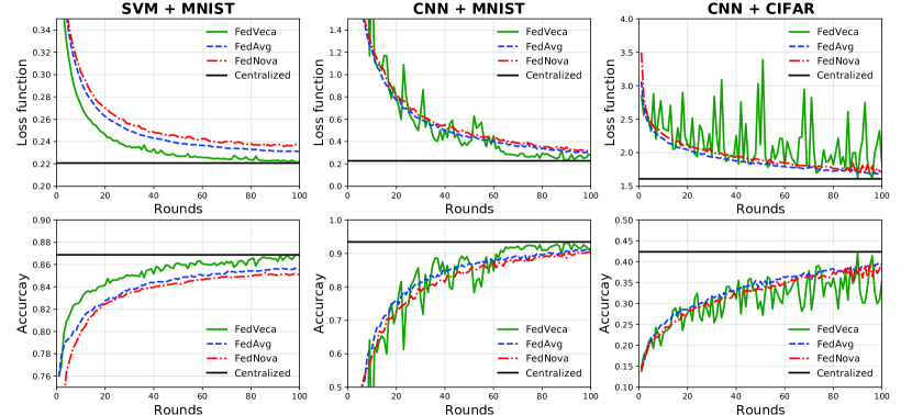
Figure 3: Loss function values and classification accuracy values in Case 3. The curves show the results from FedVeca algorithm and the baselines with the different models and datasets

In our first set of experiments, the SVM and CNN models were trained on the prototype system with Case 3, and the results $\boldsymbol{w}_{k}$ of each round will be calculated on the test dataset with the loss function values and prediction accuracy values which we refer to as loss and accuracy in short in the following.

We record the loss and accuracy on the SVM and CNN classifiers with FedVeca algorithm (with adaptive $\tau_{(k,i)}$), and compare them to baseline approaches, where the centralized case only has one optimal value as the training result and we show a flat line across different rounds for the ease of comparison, the results are shown in Fig. 3.

It can be observed from Fig. 3 that the curves of loss and accuracy values of FedVeca algorithm fluctuate less on the SVM model, while they have larger fluctuations on the CNN model. This is because the loss function of the SVM model satisfies Assumption 1 of a convex function and the loss function of the CNN model is non-convex, as we mentioned in Section IV-A2. Since the loss function of the CNN model is non-convex, the variation (orientation and size) of the local model parameters are unstable when making updates, so it is unreliable for us to describe the overall variation of global model parameters with the estimated values of $L$, $\beta_{(k,i)}$ and $\delta_{(k,i)}$. Further, it is less useful to predict the number of local SGD iterations for the next round based on the new value of $\tau_{(k,i)}$ calculated from these estimated values. However, within the specified number of rounds ($K=100$), FedVeca algorithm is the first to reach the loss and accuracy of the centralized SGD approach compared to FedAvg and FedNova on all models and datasets, demonstrating the convergence and faster convergence speed of FedVeca algorithm with Non-IID datasets.

IV-B2 Premise of Theorem 1

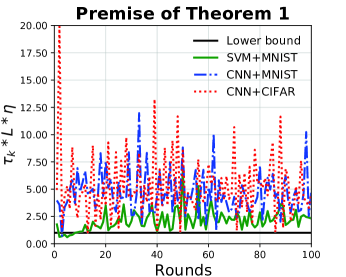
Figure 4: The value of $\eta\tau_{k}L$ in Case 3. The curves show the results from FedVeca algorithm with the different models and datasets

As described in Section III-A, the premise for Theorem 1 to be valid is that $\eta\tau_{k}L-1\geq 0$. Therefore, we record the value of $\eta\tau_{k}L$ for each round within the specified number of rounds ($K=100$) on all specified models and datasets in Case 3, the results are shown in Fig. 4.

In Fig. 4, we set the value ‘$1$’ as a lower bound on the value of $\eta\tau_{k}L$ and use a straight line to represent. Moreover, according to the discussion in Section III-B2, the estimated value of $L_{k}$ in Algorithm 1 is delayed by one round, so we make a blank for $k=0$ in Fig. 4. As we can see, the specified models and datasets satisfy the premise of Theorem 1 for all $K$ rounds, except for the SVM model whose the values of $\eta\tau_{k}L$ are slightly smaller than the lower bound for the first few rounds on the MNIST dataset (which is within the estimation margin of error). And the SVM model has the most stable $\eta\tau_{k}L$ values on the MNIST dataset compared to the other specified models and datasets, which is consistent with our conclusion that non-convex loss functions cannot be described accurately as discussed in Section IV-B1.

Due to the high complexity of evaluating CNN models, we focus on the SVM model in the following and provide further insights on the prototype system.

IV-B3 Dataset Distribution

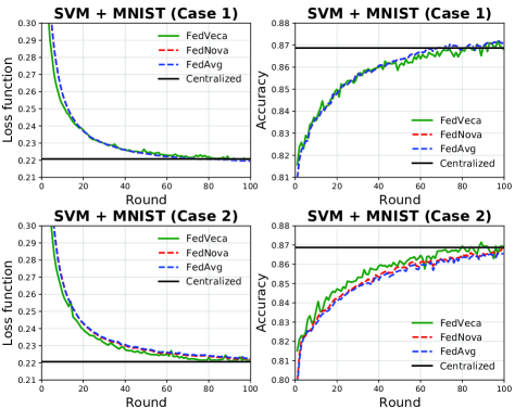
Figure 5: Loss function and classification accuracy on the SVM model and the MNIST dataset with dataset distriburion of Case 1 and Case 2.

We test the MNIST dataset distribution on the SVM model for the other two simulations which are Case 1 and Case 2, and the results of FedVeca algorithm and the baselines are shown in Fig. 5.

In Case 1, the curves of loss and accuracy values of FedVeca algorithm in each round overlap with those of FedAvg and FedNova, and both converge within $K=100$ rounds (compared to Centralized SGD), proving that FedVeca algorithm is applicable on the IID dataset. In Case 2, FedVeca algorithm has a smaller difference in loss values and a larger difference in accuracy values in each round compared to FedAvg and FedNova, and both loss and accuracy values are the first to reach the convergence point. Together with the results of Case 3 we obtained in Section IV-B1, we show that FedVeca algorithm is also applicable to the Non-IID dataset.

By comparing Fig. 5 and Fig. 3, we note that on the SVM model and the MNIST dataset (convex loss function), the convergence rate of the model obtained by FedVeca algorithm is essentially the same in Case 1, Case 2 and Case 3. Meanwhile, the models obtained by FedNova and FedAvg perform better in Case1 and Case2 and worse in Case3. This proves that FedVeca algorithm has good performance and stability on both IID and Non-IID datasets. Therefore, we focus on Case 3 in the following and provide further insights on the prototype system.

IV-B4 Instantaneous Behavior

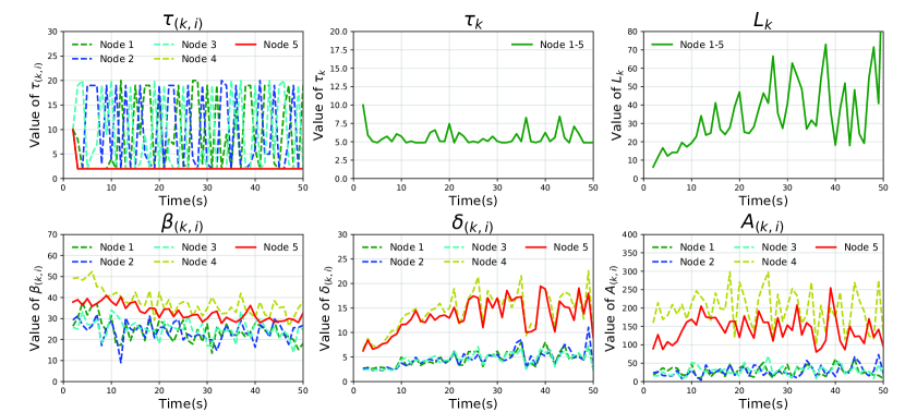
Figure 6: Instantaneous results of a single run (SVM + MNIST) with FedVeca algorithm in Case 3.

We study the instantaneous behavior of FedVeca algorithm for a single run on the prototype system. Results for SVM (MNIST) are shown in Fig. 6, where we record the amount of variation $\tau_{(k,i)}$, $\tau_{k}$, $L_{k}$ , $\beta_{(k,i)}$, $\delta_{(k,i)}$ and $A_{(k,i)}$ on the five clients, and represent only one curve for $\tau_{k}$ and $L_{k}$. To make the image clearer, we only captured the first 50 rounds of the show.

We can see that the value of $\tau_{(k,i)}$ fluctuates very much with round $k$, and the maximum number of SGD iterations in each round is uniformly distributed across clients, indicating that FedVeca algorithm can adaptively choose the optimal $\tau_{(k,i)}$ value according to the working conditions during the training process. $\tau_{k}$ represents the step size of global gradient descent in Section II-B2, and there is no large fluctuation in the curve of $\tau_{k}$, indicating that the model converges smoothly globally despite the large difference in $\tau_{(k,i)}$ values at each client under adaptive control. For the value of $L_{k}$ and Assumption 1, we know that as the number of rounds increases, the variation between the model parameters of adjacent rounds becomes smaller, which represents the convergence of the model.

According to Theorem 2, $A_{(k,i)}$ is the key variable for adaptive control of $\tau_{(k,i)}$ values and $A_{(k,i)}$ is composed of two variables, $\beta_{(k,i)}$ and $\delta_{(k,i)}$. In Fig. 6, we can see that the values of $A_{(k,i)}$ on Node 4 and Node 5 are widely spaced compared to those on the remaining three clients. This is related to the Case 3 we mentioned in Section IV-A3. The data distribution on Node 4 and Node 5 are similar but differ significantly from the remaining three clients, causing differences between the $\beta_{(k,i)}$ and $\delta_{(k,i)}$ values. Therefore, FedVeca algorithm accurately quantifies these differences and adaptively optimizes the FL training process by controlling the $\tau_{(k,i)}$ values.

IV-B5 Sensitivity of $\alpha_{k}$

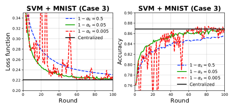
Figure 7: Loss function and classification accuracy (SVM + MNIST) with the different values of $\alpha_{k}$.

In the setup of Section IV-A4, the value of $\alpha_{k}$ is fixed for each round and we know that the maximum value of $\tau_{(k,i)}$ on all nodes in a round is related to $1-\alpha_{k}$ according to (14). Therefore, we choose three numbers 0.5, 0.05 and 0.005 for the values of $1-\alpha_{k}$ and record the variation of the model loss and accuracy values in these three scenarios, the results are shown in Fig. 7. We can see that when $1-\alpha_{k}=0.5$, the loss and accuracy curves of the model are smooth, but their convergence rate is slow. When $1-\alpha_{k}=0.005$, the loss and accuracy values of the model reach the convergence point first, but their curves are not smooth. Therefore, in our previous experiments, we chose $1-\alpha_{k}=0.05$ which means $\alpha_{k}=0.95$. In this setting, the loss and accuracy values of the model have both a fast convergence rate and a smooth curve.

IV-B6 Varying Number of clients

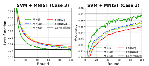
Figure 8: Loss function and classification accuracy (SVM + MNIST) with the different number of clients.

To simulate the case of multiple nodes, we let each Raspberry Pi 4B in the prototype system run multiple programs of Algorithm 2 in parallel and set the number of programs running on each Raspberry Pi 4B to be equal from 1 to 10, thus simulating the number of nodes from 5 to 50. We record the loss and accuracy values in Case 3, where the number of clients is chosen to be 5, 30 and 50 for FedVeca algorithm, FedNova and FedAvg selected the number of clients as 50, and the results are shown in Fig. 8.

We can observe that the loss and accuracy values of the model do not converge faster as the number of clients increases, which is consistent with the phenomenon of diminishing returns which is described in [3]. Also, since the size of our total training dataset is fixed, when the number of nodes increases, the number of samples on each node decreases and the data becomes more dispersed, thus reducing the speed of model convergence. However, even at 50 nodes, the model of FedVeca algorithm converges faster than FedAvg and FedNova approach, proving that FedVeca algorithm is applicable at multiple nodes.

Considering the overall experiments, we can conclude that FedVeca algorithm provides an efficient performance for FL, and provides a novel innovation with theory for FL optimization.

V Conclusion and The Future Work

In order to improve the efficiency of federated learning on the Non-IID dataset, this paper proposed an method that is based on FedNova algorithm and controls the number of local SGD iterations on clients to obtain the optimal global training models in each communication round. We analyze the mathematical relationships between the number of local SGD iterations and the global objective in a round, and design an adaptive control algorithm from this relationship to predict the number of local SGD iterations on each client for the next round. Our experimental results confirmed the effectiveness of FedVeca method. In the future, we will explore how FedVeca method performs on the models with no-convex loss functions, and assign more effective weights for updating the global model based on the number and feature of samples per client.

Appendix A Proof of Theorem 1

A-A Preliminaries

Because each global gradient is Lipschitz smooth according to the Assumption 1, and we have

$$f(\boldsymbol{x})-f(\boldsymbol{y})-\nabla f(\boldsymbol{y})^{T}(\boldsymbol{x}-\boldsymbol{y})\leq\frac{L}{2}\|\boldsymbol{x}-\boldsymbol{y}\|^{2}$$ (16)

for arbitrary $\boldsymbol{x}$ and $\boldsymbol{y}$ [38], where $\nabla f(\boldsymbol{.})^{T}$ is the transpose of $\nabla f(\boldsymbol{.})$. Thus, for $k\in[0,k-1]$, we have

$$F\left(\boldsymbol{w}_{k+1}\right)-F\left(\boldsymbol{w}_{k}\right)$$ (17)

$$\leq -\nabla F\left(\boldsymbol{w}_{k}\right)\left(\boldsymbol{w}_{k+1}-\boldsymbol{w}_{k}\right)+\frac{L}{2}\left\|\boldsymbol{w}_{k+1}-\boldsymbol{w}_{k}\right\|^{2}.$$

Substituting (5) into (17) yields

$$F\left(\boldsymbol{w}_{k+1}\right)-F\left(\boldsymbol{w}_{k}\right)$$ (18)

$$\leq -\eta\tau_{k}\left\langle\nabla F\left(\boldsymbol{w}_{k}\right),\boldsymbol{d}_{k}\right\rangle+\frac{\eta^{2}\tau_{k}^{2}L}{2}\left\|\boldsymbol{d}_{k}\right\|^{2}.$$

We solve for the inner product term of (18) to obtain

$$\left\langle\nabla F\left(\boldsymbol{w}_{k}\right),\boldsymbol{d}_{k}\right\rangle$$ (19)

$$= \frac{1}{2}\left\|\nabla F\left(\boldsymbol{w}_{k}\right)\right\|^{2}+\frac{1}{2}\left\|\boldsymbol{d}_{k}\right\|^{2}-\frac{1}{2}T_{k},$$

where $T_{k}\triangleq\left\|\nabla F\left(\boldsymbol{w}_{k}\right)-\boldsymbol{d}_{k}\right\|^{2}$ and the equation uses the fact $2\left\langle a,b\right\rangle=\left\|a\right\|^{2}+\left\|b\right\|^{2}-\left\|a-b\right\|^{2}$. Substituting (19) into (18) yields

$$\frac{F\left(\boldsymbol{w}_{k+1}\right)-F\left(\boldsymbol{w}_{k}\right)}{\eta\tau_{k}}$$ (20)

$$\leq -\frac{1}{2}\left(\left\|\nabla F\left(\boldsymbol{w}_{k}\right)\right\|^{2}+\left\|\boldsymbol{d}_{k}\right\|^{2}-T_{k}\right)+\frac{\eta\tau_{k}L}{2}\left\|\boldsymbol{d}_{k}\right\|^{2}$$

$$= -\frac{1}{2}\left\|\nabla F\left(\boldsymbol{w}_{k}\right)\right\|^{2}+\frac{\left(\eta\tau_{k}L-1\right)}{2}\left\|\boldsymbol{d}_{k}\right\|^{2}+\frac{1}{2}T_{k}$$

$$\leq (\frac{\eta\tau_{k}L}{2}-1)\left\|\nabla F\left(\boldsymbol{w}_{k}\right)\right\|^{2}+\frac{1}{2}T_{k}$$

$$\text{(when $\eta\tau_{k}L-1\geq 0$)},$$

where the last inequality is because $\left\|\boldsymbol{d}_{k}\right\|^{2}\leq\left\|\nabla F\left(\boldsymbol{w}_{k}\right)\right\|^{2}$ according to the Assumption 2. Next we will convert $T_{k}$ to contain only the similar items of $\left\|\nabla F\left(\boldsymbol{w}_{k}\right)\right\|^{2}$.

A-B Results for $T_{k}$

According to the definition of $T_{k}$ and $\boldsymbol{d}_{k}$ for $i\in[1,N]$ and $k\in[0,K-1]$, we always have

$$T_{k} =\left\|\nabla F\left(\boldsymbol{w}_{k}\right)-\sum_{i=1}^{N}p_{i}\boldsymbol{G}_{(k,i)}\right\|^{2}$$ (21)

$$=\left\|\sum_{i=1}^{N}p_{i}\left(\nabla F_{i}\left(\boldsymbol{w}_{k}\right)-\boldsymbol{G}_{(k,i)}\right)\right\|^{2}$$

(from the definition of $$\nabla F\left(\boldsymbol{w}_{k}\right)$$ in (8))

$$\leq\sum_{i=1}^{N}p_{i}\left\|\nabla F_{i}\left(\boldsymbol{x}_{k}\right)-\boldsymbol{G}_{(k,i)}\right\|^{2},$$

where the last inequality uses Jensen’s Inequality: $\left\|\sum_{i=1}^{N}\varphi_{i}\boldsymbol{z}\right\|^{2}\leq\sum_{i=1}^{N}\varphi_{i}\left\|\boldsymbol{z}\right\|^{2}$ for arbitrary $\boldsymbol{z}$ and $\sum_{i=1}^{N}\varphi_{i}=1$. Then, we solve for $\left\|\nabla F_{i}\left(\boldsymbol{x}_{k}\right)-\boldsymbol{G}_{(k,i)}\right\|^{2}$ and get

$$\left\|\nabla F_{i}\left(\boldsymbol{w}_{k}\right)-\boldsymbol{G}_{(k,i)}\right\|^{2}$$ (22)

$$=\left\|\nabla F_{i}\left(\boldsymbol{w}_{k}\right)-\frac{1}{\tau_{(k,i)}}\sum_{\lambda=0}^{\tau_{(k,i)}-1}\nabla F_{i}\left(\boldsymbol{w}_{(k,i)}^{\lambda}\right)\right\|^{2}$$

$$=\left\|\sum_{\lambda=0}^{\tau_{(k,i)}-1}\frac{1}{\tau_{(k,i)}}\left(\nabla F_{i}\left(\boldsymbol{w}_{k}\right)-\nabla F_{i}\left(\boldsymbol{w}_{(k,i)}^{\lambda}\right)\right)\right\|^{2}$$

$$\leq\sum_{\lambda=0}^{\tau_{(k,i)}-1}\frac{1}{\tau_{(k,i)}}\left\|\nabla F_{i}\left(\boldsymbol{w}_{k}\right)-\nabla F_{i}\left(\boldsymbol{w}_{(k,i)}^{\lambda}\right)\right\|^{2}$$

(from Jensen’s Inequality)

$$\leq\sum_{\lambda=0}^{\tau_{(k,i)}-1}\frac{\beta_{(k,i)}^{2}}{\tau_{(k,i)}}\left\|\boldsymbol{w}_{k}-\boldsymbol{w}_{(k,i)}^{\lambda}\right\|^{2}$$

(from the Assumption 3)

for $\lambda\in[0,\tau_{(k,i)}-1]$. According to our definition in Section II, we have $\boldsymbol{w}_{k}=\boldsymbol{w}_{(k,i)}^{\lambda}$ at $\lambda=0$, at this point the last term of the inequation in (22) has $\left\|\boldsymbol{w}_{k}-\boldsymbol{w}_{(k,i)}^{0}\right\|^{2}=0$. Therefore, we solve for $\left\|\boldsymbol{w}_{k}-\boldsymbol{w}_{(k,i)}^{\lambda}\right\|^{2}$ with $\lambda\in[1,\tau_{(k,i)}-1]$ and obtain

$$\left\|\boldsymbol{w}_{k}-\boldsymbol{w}_{(k,i)}^{\lambda}\right\|^{2}=\eta^{2}\left\|\sum_{s=0}^{\lambda-1}\nabla F_{i}\left(\boldsymbol{w}_{(k,i)}^{s}\right)\right\|^{2}$$ (23)

(from the SGD rule in (1))

$$\leq \eta^{2}\delta_{(k,i)}\sum_{s=0}^{\lambda-1}\left\|\nabla F\left(\boldsymbol{w}_{k}\right)\right\|^{2}$$

(from the Assumption 4)

$$= \eta^{2}\delta_{(k,i)}\lambda\left\|\nabla F\left(\boldsymbol{w}_{k}\right)\right\|^{2}.$$

Substituting (23) into (23), we get

$$\left\|\nabla F_{i}\left(\boldsymbol{w}_{k}\right)-\boldsymbol{G}_{(k,i)}\right\|^{2}$$ (24)

$$\leq \sum_{\lambda=0}^{\tau_{(k,i)}-1}\lambda\eta^{2}\frac{\beta_{(k,i)}^{2}\delta_{(k,i)}}{\tau_{(k,i)}}\left\|\nabla F\left(\boldsymbol{w}_{k}\right)\right\|^{2}$$

$$= \frac{\tau_{(k,i)}-1}{2}\eta^{2}\beta_{(k,i)}^{2}\delta_{(k,i)}\left\|\nabla F\left(\boldsymbol{w}_{k}\right)\right\|^{2}$$

$$= \frac{\tau_{(k,i)}-1}{2}\eta A_{(k,i)}\left\|\nabla F\left(\boldsymbol{w}_{k}\right)\right\|^{2}$$

(from the definition that $$A_{(k,i)}\triangleq\eta\beta_{(k,i)}^{2}\delta_{(k,i)})$$.

Substituting (24) into (21), we get

$$T_{k} \leq\sum_{i=1}^{N}p_{i}\frac{\tau_{(k,i)}-1}{2}\eta A_{(k,i)}\left\|\nabla F\left(\boldsymbol{w}_{k}\right)\right\|^{2}$$ (25)

$$=\frac{1}{2}\eta\left\|\nabla F\left(\boldsymbol{w}_{k}\right)\right\|^{2}\sum_{i=1}^{N}p_{i}(\tau_{(k,i)}-1)A_{(k,i)}.$$

Now, we are ready to derive the final result.

A-C Final Result

Plugging (25) back into (20), we have

$$\frac{F\left(\boldsymbol{w}_{k+1}\right)-F\left(\boldsymbol{w}_{k}\right)}{\eta\tau_{k}}$$ (26)

$$\leq (\frac{\eta\tau_{k}L}{2}-1)\left\|\nabla F\left(\boldsymbol{w}_{k}\right)\right\|^{2}+$$

$$\frac{1}{4}\eta\left\|\nabla F\left(\boldsymbol{w}_{k}\right)\right\|^{2}\sum_{i=1}^{N}p_{i}(\tau_{(k,i)}-1)A_{(k,i)}$$

$$= \left\|\nabla F\left(\boldsymbol{w}_{k}\right)\right\|^{2}\left(-1+\frac{1}{4}\eta(2\tau_{k}L+\sum_{i=1}^{N}p_{i}(\tau_{(k,i)}-1)A_{(k,i)})\right)$$

$$= \left(-1+\frac{1}{4}\eta(\sum_{i=1}^{N}p_{i}\tau_{(k,i)}2L+\sum_{i=1}^{N}p_{i}(\tau_{(k,i)}-1)A_{(k,i)})\right)$$

$$\left\|\nabla F\left(\boldsymbol{w}_{k}\right)\right\|^{2}$$

(from the defition of $$\tau_{k}$$ in (5))

$$= \left(\frac{1}{4}\eta\sum_{i=1}^{N}p_{i}\left(\tau_{(k,i)}\left(2L+A_{(k,i)}\right)-A_{(k,i)}\right)-1\right)\left\|\nabla F\left(\boldsymbol{w}_{k}\right)\right\|^{2}.$$

Appendix B Proof of Theorem

From Theorem 1 we get that $\eta\tau_{k}L-1\geq 0$ which means $\eta\sum_{i=1}^{N}p_{i}(\tau_{(k,i)}L\geq 1$ in the $k$-th round ($k\in[0,k-1]$). Thus, it exists a real number $\varepsilon_{k}$ such that

$$\frac{1}{4}\left(\varepsilon_{k}+2\right)\eta\sum_{i=1}^{N}p_{i}(\tau_{(k,i)}L<1.$$ (27)

Obviously, $\varepsilon_{k}<2$, because when $\varepsilon_{k}\geq 2$, we have a self-contradictory inequality $\frac{1}{4}\left(\varepsilon_{k}+2\right)\eta\sum_{i=1}^{N}p_{i}(\tau_{(k,i)}L\geq\eta\sum_{i=1}^{N}p_{i}(\tau_{(k,i)}L\geq 1$. And to ensure the model convergence in Theorem 1 we have

$$\frac{1}{4}\eta\sum_{i=1}^{N}p_{i}\left(\tau_{(k,i)}\left(2L+A_{(k,i)}\right)-A_{(k,i)}\right)$$ (28)

$$\leq \frac{1}{4}\left(\varepsilon_{k}+2\right)\eta\sum_{i=1}^{N}p_{i}(\tau_{(k,i)}L$$

$$= \frac{1}{4}\eta\sum_{i=1}^{N}p_{i}(\tau_{(k,i)}L\left(\varepsilon_{k}+2\right).$$

In order for the inequality (28) to hold, we have

$$\tau_{(k,i)}\left(2L+A_{(k,i)}\right)-A_{(k,i)}\leq\tau_{(k,i)}L\left(\epsilon_{k}+2\right)$$ (29)

$$\tau_{(k,i)}\left(A_{(k,i)}-\epsilon_{k}L\right)\leq A_{(k,i)}$$

(when $$A_{(k,i)}-\epsilon_{k}L>0$$)

$$\tau_{(k,i)}\leq\frac{A_{(k,i)}}{A_{(k,i)}-\epsilon_{k}L}.$$

Since we set the lower bound of $\tau_{(k,i)}>1$, we have $\frac{A_{(k,i)}}{A_{(k,i)}-\epsilon_{k}L}>1$ which is equivalent to $\epsilon_{k}>0$, and get $\varepsilon_{k}\in(0,2)$. Then, we define the existence of another real number $\alpha_{k}$ that

$$\epsilon_{k}L=\alpha_{k}\min_{i}A_{(k,i)}.$$ (30)

We know that $\alpha_{k}=\frac{\epsilon_{k}L}{\min_{i}A_{(k,i)}}$, thus $\alpha_{k}\in(0,\frac{2L}{\min_{i}A_{(k,i)}})$. To ensure that $A_{(k,i)}-\epsilon_{k}L>0$ is established, we impose further constraints on $\epsilon_{k}$ that $\alpha_{k}\in(0,\frac{2L}{\min_{i}A_{(k,i)}})$ (when $\frac{2L}{\min_{i}A_{(k,i)}}<1$) and $\alpha_{k}\in(0,1)$ (when $\frac{2L}{\min_{i}A_{(k,i)}}>1$). Substituting (29) into (30), we get

$$\tau_{(k,i)}\leq\frac{A_{(k,i)}}{A_{(k,i)}-\alpha_{k}\min_{i}A_{(k,i)}}.$$ (31)

References

- [1] J. Konečnỳ, H. B. McMahan, F. X. Yu, P. Richtárik, A. T. Suresh, and D. Bacon, “Federated learning: Strategies for improving communication efficiency,” arXiv preprint arXiv:1610.05492, 2016.
- [2] J. Liu, J. Huang, Y. Zhou, X. Li, S. Ji, H. Xiong, and D. Dou, “From distributed machine learning to federated learning: A survey,” Knowledge and Information Systems, pp. 1–33, 2022.
- [3] B. McMahan, E. Moore, D. Ramage, S. Hampson, and B. A. y Arcas, “Communication-efficient learning of deep networks from decentralized data,” in Artificial intelligence and statistics. PMLR, 2017, pp. 1273–1282.
- [4] J. Wang and G. Joshi, “Cooperative sgd: A unified framework for the design and analysis of local-update sgd algorithms,” Journal of Machine Learning Research, vol. 22, 2021.
- [5] P. Dvurechensky, A. Gasnikov, and A. Kroshnin, “Computational optimal transport: Complexity by accelerated gradient descent is better than by sinkhorn’s algorithm,” in International conference on machine learning. PMLR, 2018, pp. 1367–1376.
- [6] Y. Lei, T. Hu, G. Li, and K. Tang, “Stochastic gradient descent for nonconvex learning without bounded gradient assumptions,” IEEE transactions on neural networks and learning systems, vol. 31, no. 10, pp. 4394–4400, 2019.
- [7] N. J. Harvey, C. Liaw, Y. Plan, and S. Randhawa, “Tight analyses for non-smooth stochastic gradient descent,” in Conference on Learning Theory. PMLR, 2019, pp. 1579–1613.
- [8] M. Aledhari, R. Razzak, R. M. Parizi, and F. Saeed, “Federated learning: A survey on enabling technologies, protocols, and applications,” IEEE Access, vol. 8, pp. 140 699–140 725, 2020.
- [9] F. Sattler, S. Wiedemann, K.-R. Müller, and W. Samek, “Robust and communication-efficient federated learning from non-iid data,” IEEE transactions on neural networks and learning systems, vol. 31, no. 9, pp. 3400–3413, 2019.
- [10] M. Luo, F. Chen, D. Hu, Y. Zhang, J. Liang, and J. Feng, “No fear of heterogeneity: Classifier calibration for federated learning with non-iid data,” Advances in Neural Information Processing Systems, vol. 34, pp. 5972–5984, 2021.
- [11] P. Zhang, H. Sun, J. Situ, C. Jiang, and D. Xie, “Federated transfer learning for iiot devices with low computing power based on blockchain and edge computing,” Ieee Access, vol. 9, pp. 98 630–98 638, 2021.
- [12] H. Zhu, J. Xu, S. Liu, and Y. Jin, “Federated learning on non-iid data: A survey,” Neurocomputing, vol. 465, pp. 371–390, 2021.
- [13] T. Yoon, S. Shin, S. J. Hwang, and E. Yang, “Fedmix: Approximation of mixup under mean augmented federated learning,” in International Conference on Learning Representations, 2020.
- [14] H. Zhang, M. Cisse, Y. N. Dauphin, and D. Lopez-Paz, “mixup: Beyond empirical risk minimization,” in International Conference on Learning Representations, 2018.
- [15] K. Zhou, Z. Liu, Y. Qiao, T. Xiang, and C. C. Loy, “Domain generalization: A survey,” IEEE Transactions on Pattern Analysis and Machine Intelligence, 2022.
- [16] A. Back de Luca, G. Zhang, X. Chen, and Y. Yu, “Mitigating data heterogeneity in federated learning with data augmentation,” arXiv e-prints, pp. arXiv–2206, 2022.
- [17] H. Wang, Z. Kaplan, D. Niu, and B. Li, “Optimizing federated learning on non-iid data with reinforcement learning,” in IEEE INFOCOM 2020-IEEE Conference on Computer Communications. IEEE, 2020, pp. 1698–1707.
- [18] M. Yang, X. Wang, H. Zhu, H. Wang, and H. Qian, “Federated learning with class imbalance reduction,” in 2021 29th European Signal Processing Conference (EUSIPCO). IEEE, 2021, pp. 2174–2178.
- [19] Y. Zhao, M. Li, L. Lai, N. Suda, D. Civin, and V. Chandra, “Federated learning with non-iid data,” arXiv preprint arXiv:1806.00582, 2018.
- [20] T. Tuor, S. Wang, B. J. Ko, C. Liu, and K. K. Leung, “Overcoming noisy and irrelevant data in federated learning,” in 2020 25th International Conference on Pattern Recognition (ICPR). IEEE, 2021, pp. 5020–5027.
- [21] N. Yoshida, T. Nishio, M. Morikura, K. Yamamoto, and R. Yonetani, “Hybrid-fl: Cooperative learning mechanism using non-iid data in wireless networks,” arXiv preprint arXiv:1905.07210, 2019.
- [22] A. Fallah, A. Mokhtari, and A. Ozdaglar, “Personalized federated learning with theoretical guarantees: A model-agnostic meta-learning approach,” Advances in Neural Information Processing Systems, vol. 33, pp. 3557–3568, 2020.
- [23] C. Finn, P. Abbeel, and S. Levine, “Model-agnostic meta-learning for fast adaptation of deep networks,” in International conference on machine learning. PMLR, 2017, pp. 1126–1135.
- [24] C. T Dinh, N. Tran, and J. Nguyen, “Personalized federated learning with moreau envelopes,” Advances in Neural Information Processing Systems, vol. 33, pp. 21 394–21 405, 2020.
- [25] V. Smith, C.-K. Chiang, M. Sanjabi, and A. S. Talwalkar, “Federated multi-task learning,” Advances in neural information processing systems, vol. 30, 2017.
- [26] L. Corinzia, A. Beuret, and J. M. Buhmann, “Variational federated multi-task learning,” arXiv preprint arXiv:1906.06268, 2019.
- [27] F. Chen, M. Luo, Z. Dong, Z. Li, and X. He, “Federated meta-learning with fast convergence and efficient communication,” arXiv preprint arXiv:1802.07876, 2018.
- [28] Z. Zhu, J. Hong, and J. Zhou, “Data-free knowledge distillation for heterogeneous federated learning,” in International Conference on Machine Learning. PMLR, 2021, pp. 12 878–12 889.
- [29] T. Lin, L. Kong, S. U. Stich, and M. Jaggi, “Ensemble distillation for robust model fusion in federated learning,” Advances in Neural Information Processing Systems, vol. 33, pp. 2351–2363, 2020.
- [30] X. Peng, Z. Huang, Y. Zhu, and K. Saenko, “Federated adversarial domain adaptation,” arXiv preprint arXiv:1911.02054, 2019.
- [31] J. Wang, Q. Liu, H. Liang, G. Joshi, and H. V. Poor, “Tackling the objective inconsistency problem in heterogeneous federated optimization,” Advances in neural information processing systems, vol. 33, pp. 7611–7623, 2020.
- [32] T. Li, A. K. Sahu, M. Zaheer, M. Sanjabi, A. Talwalkar, and V. Smith, “Federated optimization in heterogeneous networks,” Proceedings of Machine Learning and Systems, vol. 2, pp. 429–450, 2020.
- [33] X. Liang, S. Shen, J. Liu, Z. Pan, E. Chen, and Y. Cheng, “Variance reduced local sgd with lower communication complexity,” arXiv preprint arXiv:1912.12844, 2019.
- [34] S. P. Karimireddy, S. Kale, M. Mohri, S. Reddi, S. Stich, and A. T. Suresh, “Scaffold: Stochastic controlled averaging for federated learning,” in International Conference on Machine Learning. PMLR, 2020, pp. 5132–5143.
- [35] S. Wang, T. Tuor, T. Salonidis, K. K. Leung, C. Makaya, T. He, and K. Chan, “Adaptive federated learning in resource constrained edge computing systems,” IEEE Journal on Selected Areas in Communications, vol. 37, no. 6, pp. 1205–1221, 2019.
- [36] Y. LeCun, L. Bottou, Y. Bengio, and P. Haffner, “Gradient-based learning applied to document recognition,” Proceedings of the IEEE, vol. 86, no. 11, pp. 2278–2324, 1998.
- [37] A. Krizhevsky et al., “Learning multiple layers of features from tiny images,” 2009.
- [38] S. Bubeck et al., “Convex optimization: Algorithms and complexity,” Foundations and Trends® in Machine Learning, vol. 8, no. 3-4, pp. 231–357, 2015.