Consensus Knowledge Graph Learning via Multi-view Sparse Low Rank Block Model

Abstract

Network analysis has been a powerful tool to unveil relationships and interactions among a large number of objects. Yet its effectiveness in accurately identifying important node-node interactions is challenged by the rapidly growing network size, with data being collected at an unprecedented granularity and scale. Common wisdom to overcome such high dimensionality is collapsing nodes into smaller groups and conducting connectivity analysis on the group level. Dividing efforts into two phases inevitably opens a gap in consistency and drives down efficiency. Consensus learning emerges as a new normal for common knowledge discovery with multiple data sources available. To this end, this paper features developing a unified framework of simultaneous grouping and connectivity analysis by combining multiple data sources. The algorithm also guarantees a statistically optimal estimator.

Key words: multi-view, consensus network, low-rank block model, sparse random effect

1 Introduction

Network analysis that unveils connectivity and interactions among a large number of objects is a problem of great importance with wide applications in social sciences, genomics, clinical medicine, and beyond [Goh et al., 2007, Nabieva et al., 2005, Luscombe et al., 2004, Scott, 1988, e.g.]. As data are being collected at an unprecedented granularity and scale, it is now possible to study the structure of large networks. However, it is challenging to accurately infer the network structure in the presence of high dimensionality, especially when many nodes represent highly similar entities and multiple data sources are available. A simple approach to overcome the high dimensionality and overlapping entities is to collapse similar nodes into groups. With groupings given as a priori, network connectivity analysis is subsequently performed on the group level to improve interpretability and reproducibility. For example, inferences for gene regulatory networks in genomics are often made on the pathway level that generally represents a group of functionally related genes [Kelley and Ideker, 2005, Xia et al., 2018, e.g]. Brain function network analyses are often performed on groups of voxels localized within a small region having a common neurological function [Shaw et al., 2007, Chen et al., 2017, Lu et al., 2017, e.g.]. However, for many applications, group structure is unknown and needs to be estimated together with the network structure. In natural language processing (NLP), synonymous terms should be grouped yet such grouping structure varies by context and is not generally available. In association studies linking current procedural terminology (CPT) codes to clinical outcomes, many procedures are clinically equivalent yet currently available grouping of CPT codes is extremely crude [Agency for Healthcare Research and Quality, 2019].

Despite the potential large sample size, network structure inferred from a single data source is susceptible to biases associated with the population or mechanism the data is generated from. As more data sources become available, it is highly desirable to synthesize information from multiple sources, often termed as views, to jointly infer about a consensus network structure. This debiasing for common knowledge discovery is particularly important when dealing with inherently heterogeneous data sources. A prime example comes from knowledge extraction using Electronic Health Records (EHR) data. The EHR system contains rich longitudinal phenotypic information from millions of patients. The EHR data is a valuable source to learn medical knowledge network linking each specific disease condition with co-morbidities, diagnostic laboratory measurements, procedures, and treatment. Constructing a consensus network using data from multiple EHR systems could potentially remove bias due to different patient populations, physician training and practices, as well as how or when the encodings are performed. However, the between view heterogeneity also imposes methodological challenges to accurately learning network structure.

To overcome these challenges, we propose in this paper a unified framework that can efficiently combine multi-view data to simultaneously group entities and infer about network structure. Specifically, we aim to learn a consensus network that reflects shared knowledge using a collection of $m$ independently-observed graphs on $n$ common vertex set ${\cal V}=\{v_{j}\}_{j\in[n]}$,

$${\cal G}_{[m]}=\Big{\{}{\cal G}_{s}=\{{\cal V},\mathbf{W}_{s}\}:{\cal V}=\{v_{j}\}_{j\in[n]},\mathbf{W}_{s}=\big{[}W_{s}(j_{1},j_{2})\big{]}_{j_{1}\in[n]}^{j_{2}\in[n]}\Big{\}}_{s\in[m]}\,,$$

where $[n]=\{1,\cdots,n\}$, and $W_{s}(j_{1},j_{2})$ is the observed edge weight between node $v_{j_{1}}$ and node $v_{j_{2}}$ from the $s^{\rm th}$ view. The vertex set ${\cal V}$ admits a latent grouping structure shared across $m$ views in that there exists a unique non-overlapping $K$-partition:

$${\cal V}=\cup_{k=1}^{K}{\cal V}_{k},{\cal V}_{k}\cap{\cal V}_{l}=\emptyset,\forall 1\leq k<l\leq K,$$

which can be equivalently represented by a 0/1 matrix $\mathbf{Z}=\big{[}Z(j,k)\big{]}_{j\in[n]}^{k\in[K]},\mbox{where }Z(j,k)=I(v_{j}\in{\cal V}_{k})$. To model the network structure while accommodating heterogeneity across views, we assume a flexible multi-view sparse low-rank model for $\{\mathbf{W}_{s}\}_{s=1}^{m}$ which shares a sparse consensus matrix $\mathbf{C}$ that captures the shared network structure and components capturing heterogeneity in both the network structure and information content. The consensus matrix $\mathbf{C}$ can be further decomposed into $\mathbf{C}=\mathbf{Z}\mathbf{\Omega}\mathbf{Z}^{\top}$, where $\mathbf{\Omega}$ is a group-level sparse and low rank weight matrix. Our goal is to simultaneously learn $\mathbf{Z}$ and $\mathbf{C}$ from ${\cal G}_{[m]}$ in the presence of heterogeneity.

The proposed framework is particularly appealing for knowledge graph modeling with multi-view data for several reasons. To illustrate this, consider our motivating example of knowledge extraction with multi-view EHR data where the nodes represent clinical concepts including disease conditions, signs/symptoms, diagnostic laboratory tests, procedures and treatments. First, nodes within a group can effectively represent stochastically equivalent and interchangeable medical terms. For example, the clinical concepts “coronary artery disease” and “coronary heart disease” are used interchangeably by physicians but are mapped to two separate clinical concept unique identifies in the unified medical language system (UMLS) [Bodenreider, 2004]. Second, the structure of the group level dependency captured by $\mathbf{\Omega}$ can be used to infer about clinical knowledge about a disease. The consensus graph is particularly appealing as it removes biases from individual healthcare systems. Third, the improved estimation of the low rank weight matrix $\mathbf{\Omega}$ and $\mathbf{Z}$ through consensus learning also leads to a more accurate embedding representation for the nodes.

In a special case that $\mathbf{\Omega}$ is full-rank and each entry is non-negative and upper bounded by $1$, $\mathbf{W}$ reduces to the well known stochastic block model (SBM) [Holland et al., 1983] since $\mathbf{W}$ characterizes the underlying Bernoulli distribution for entries in the observed adjacency matrix. More broadly, recovering $\mathbf{\Omega}$ shows a direct effort tapping into the network dynamics. For example, for clinical practices, complex diseases are often accompanied by a series of symptoms that may need multiple concurrent treatments. Therefore, learning a knowledge network of disease would greatly help support decision making toward precision medicine. Lastly, the decomposition on $\mathbf{W}$ embodies efficient vector representations that enable groups of nodes embeddings. This provides a new embedding technique applicable in many areas, such as proteins, DNA sequences, fMRI, to expand their existing embedding family serving for broader research needs [Asgari and Mofrad, 2015, Nguyen et al., 2016, Choi et al., 2016, Ng, 2017, Vodrahalli et al., 2018, e.g.].

With a single view, a simple approach to achieve this goal is to first perform grouping based on scalable clustering algorithms [Shi and Malik, 2000, Ng et al., 2002, Newman, 2006, Bickel and Chen, 2009, Zhao et al., 2012, e.g.] and then learn the network structure. However, dividing efforts into two phases inevitably opens a gap that could potentially create frictions in consistency and drive down efficiency with transmitting information. For the sole purpose of recovering $\mathbf{Z}$, SBM is perhaps one of the most developed frameworks that enjoys both straightforward interpretations and good statistical properties [Rohe et al., 2011, Lei and Rinaldo, 2015, Nielsen and Witten, 2018, Abbe, 2018, Gao et al., 2017, e.g.]. Central to SBM is the idea that the observed adjacency matrix is a noisy version of a rank-$K$ matrix with eigenvectors having exactly $K$ unique rows. Each unique row can be comprehended as a $K$-dimensional vector representation for nodes in the $K^{\rm th}$ group. However, this assumption becomes too restrictive requiring the embedding dimension $r$ be tied to the number of groups $K$. As $K$ grows (potentially with $n$), the embedding dimension desirably remains low. To this end, we generalize SBM by introducing a low-rank block model (LBM) on ${\cal W}$ to allow $\mathbf{\Omega}$ to be low-rank, thus decoupling $r$ from $K$. Extending to a multi-view setting, we further introduce a multi-view sparse low-rank block model (msLBM) to jointly model the faithfulness to the consensus and view-specific varying part. One theoretical contribution in our proposed msLBM model is to perform a low-rank and sparse matrix decomposition with overlapping subspace on multiple noisy data sources.

Recent years have witnessed an fast growing literature on multi-layer network analysis [Levin et al., 2017, Le et al., 2018, Tang et al., 2017, Wang et al., 2019b, Jones and Rubin-Delanchy, 2020, Paul et al., 2020, Lei et al., 2020, Jing et al., 2021, Arroyo et al., 2021, Levin et al., 2022, e.g.]. For example, Arroyo et al. [2021] considered multiple random dot product graphs sharing a common invariant subspace and Wang et al. [2019a] decomposed the logistic-transformed multi-view expected adjacency matrices to a common part and individual low-rank matrices. Levin et al. [2022] proposed the weighted adjacency spectral embedding under the assumption that multi-layer networks share a common connectivity probability with a potential low-rank structure, while the noise distributions of different layers can be heterogeneous. Recently, MacDonald et al. [2022] proposed a latent space multiplex networks models that part of the latent representation is shared across all layers while heterogeneity is allowed for the other part.

Our msLBM model differs from those prior works in three crucial aspects. First, our msLBM allows node-wise heterogeneity on the consensus graph of each view/layer while the existing literature assumes SBM on each layer. Secondly, what is more important, our method allows view-wise heterogeneity on the consensus graph across different views/layers. This additional flexibility enables us dealing with heterogeneous data collected from different sources. Finally, our msLBM model introduces additional sparse signal on each view/layer which is unexplainable by the low-rank consensus graph. Oftentimes, these sparse signal can capture uncommon network structure in each view/layer. These new ingredients in msLBM are motivated by the uniqueness of multi-view EHR data. Meanwhile, all these differences also make it more challenging to estimate the underlying consensus graph in our msLBM.

The rest of paper is organized as follows. In Section 2, we elaborate in more details on the proposed low-rank block model and its extension accounting for heterogeneity arising in a multi-view setting. We then propose an alternating minimization based approach in Section 3 to learn the consensus network that is easy and fast to implement in practice. Section 4 provides all theoretical justifications. Simulations are given in Section 5 to demonstrate the efficacy and robustness of the proposed method. In Section 6, we apply the proposed method to generate a new set of clinical concept embeddings and yield a very insightful Disease-Symptom-Treatment network on Coronary Artery Disease, by integrating information from a large digital repository of journal articles and three healthcare systems. Proofs on theories in Section 4 are relegated to Appendix.

2 Multi-view Sparse Low-rank Block Model

2.1 Notations

Throughout, we use a boldfaced uppercase letter to denote a matrix and the same uppercase letter in normal font to represent its entries. We use a boldfaced lowercase letter to denote a vector and the same lowercase letter in normal font to represent its entries. Let $\mathbf{I}_{r}$ denote the $r\times r$ identity matrix and $\mathbf{1}_{n}$ denote the $n$-dimensional all-one vector. We let $\|\cdot\|_{\ell_{2}}$ denote vector $\ell_{2}$-norm. For any matrix $\mathbf{A}$, let $\|\mathbf{A}\|,\|\mathbf{A}\|_{\rm F}$ denote its spectral norm and Frobenius norm respectively, $\|\mathbf{A}\|_{\ell_{1}}=\sum_{i,j}|A_{i,j}|$, $\|\mathbf{A}\|_{\ell_{\infty}}=\max_{i,j}|A_{i,j}|$, $\lambda_{j}(\mathbf{A})$ denote its $j^{\rm th}$ largest singular value, $\mathbf{A}_{i:}$ and $\mathbf{A}_{:j}$ respectively denote its $i^{\rm th}$ row and $j^{\rm th}$ column, ${\rm Vec}(\mathbf{A})$ denote vectorizing $\mathbf{A}$ column by column, $\kappa(\mathbf{A})=\lambda_{1}(\mathbf{A})/\lambda_{{\rm rank}(\mathbf{A})}(\mathbf{A})$ denote the condition number of $\mathbf{A}$. For a set ${\cal V}$, we use ${\rm Card}({\cal V})$ to denote its cardinality. We denote the set of $r\times r$ orthogonal matrices by

$${\mathscr{O}}_{r,r}:=\big{\{}\mathbf{O}\in\mathbb{R}^{r\times r}:\mathbf{O}\mathbf{O}^{\top}=\mathbf{O}^{\top}\mathbf{O}=\mathbf{I}_{r}\big{\}}.$$

If the entries of an orthogonal matrix $\mathbf{O}\in{\mathscr{O}}_{r,r}$ are either $0$ or $1$ such that each row and column contains one single nonzero entry, then we call $\mathbf{O}$ a permutation matrix. The set of all $r\times r$ permutation matrices is denoted by ${\mathscr{P}}_{r,r}\subset{\mathscr{O}}_{r,r}$. With slight abuse of notations, we denote the set of $n\times K$ matrices with orthonormal columns by

$${\mathscr{O}}_{n,K}:=\big{\{}\mathbf{X}\in\mathbb{R}^{n\times K}:\mathbf{X}^{\top}\mathbf{X}=\mathbf{I}_{K}\big{\}}\,.$$

Given any matrix $\mathbf{A}\in\mathbb{R}^{n\times r}$ with ${\rm rank}(\mathbf{A})=r$, let ${\cal P}_{\mathbf{A}}$ denote the orthogonal projection from $\mathbb{R}^{n}$ to the column space of $\mathbf{A}$, or more specifically ${\cal P}_{\mathbf{A}}(\mathbf{v})=\mathbf{A}(\mathbf{A}^{\top}\mathbf{A})^{-1}\mathbf{A}^{\top}\mathbf{v}$ for any $\mathbf{v}\in\mathbb{R}^{n}$. We denote $\mathbf{e}_{j}$ the $j$-th canonical basis vector, whose dimension might change at different appearances. Denote $\mathbf{A}\circ\mathbf{B}$ the Hadamard product of matrix $\mathbf{A}$ and $\mathbf{B}$.

2.2 Low-rank Block Model (LBM)

We first introduce the graph model for a single view. Let ${\cal G}=\{{\cal V},\mathbf{W}\}$ denote an undirected weighted graph with vertex set ${\cal V}=\{v_{j}\}_{j\in[n]}$ and symmetric weight matrix $\mathbf{W}=[W(j_{1},j_{2})]_{j_{1}\in[n]}^{j_{2}\in[n]}$ with $W(j_{1},j_{2})$ representing the connection intensity between the vertices $v_{j_{1}}$ and $v_{j_{2}}$. We assume that the graph ${\cal G}$ admits a latent network structure in the sense that there exits a unique (unknown) non-overlapping $K$-partition of the vertex set ${\cal V}$:

$${\cal V}=\cup_{k=1}^{K}{\cal V}_{k},\quad{\rm Card}({\cal V}_{k})=n_{k},\quad{\cal V}_{k}\cap{\cal V}_{l}=\emptyset,\quad\forall 1\leq k<l\leq K,$$

with $n=\sum_{k=1}^{K}n_{k}$, which can be equivalently represented by a group membership matrix

$$\mathbf{Z}=\big{[}Z(j,k)\big{]}_{j\in[n]}^{k\in[K]},\quad\mbox{where}\quad Z(j,k)={\bf 1}(v_{j}\in{\cal V}_{k})\in\{0,1\}.$$

We denote by ${\mathscr{Z}}_{n,K}$ the set of all possible $n\times K$ dimensional $K$-group membership matrices for $n$ nodes. Throughout, we assume $K$ is known that can grow with $n$ for high-dimensional cases for all theoretical analyses. Strategies of choosing an appropriate $K$ would be dicussed in Section 6. The set of orthornormalized membership matrices is denoted by

$${\mathscr{U}}_{n,K}=\Big{\{}\mathbf{U}:=\mathbf{Z}\left[\mathop{\rm diag}(\mathbf{1}_{n}^{\top}\mathbf{Z})\right]^{-1/2}:\mathbf{Z}\in{\mathscr{Z}}_{n,K}\Big{\}}\subset{\mathscr{O}}_{n,K}.$$

We assume the edge weight matrix $\mathbf{W}$ can be decomposed as

$$\mathbf{W}=\mathbf{H}\mathbf{Z}\mathbf{\Omega}\mathbf{Z}^{\top}\mathbf{H}=:\mathbf{H}\mathbf{C}\mathbf{H}$$ (2.1)

where the symmetric matrix $\mathbf{\Omega}\in\mathbb{R}^{K\times K}$ is the group-level correlation matrix that measures the strength of connectivity between groups with diagonal entries being 1 and other entries bounded by $1$, and the diagonal matrix $\mathbf{H}={\rm diag}(h_{1},\cdots,h_{n})$ indexes the information content for each node contained in the view. In a special case that each entry of $\mathbf{\Omega}$ is non-negative, and $\mathbf{H}$’s entries are upper bounded by $1$, model (2.1) reduces to the degree corrected stochastic block model (DCBM,Karrer and Newman [2011]) under which $W(j_{1},j_{2})$ represents the probability of $v_{j_{1}}$ and $v_{j_{2}}$ being connected, and the matrix $\mathbf{\Omega}$ is assumed to be full-rank to recover $\mathbf{Z}$ for community detection. However, this full-rank assumption is inappropriate for knowledge graph modeling where $K$ is often large but $\mathbf{\Omega}$ is low rank. We instead assume the following a low-rank block model (LBM) as a generalization of DCBM.

Assumption 2.1 (LBM).

The graph ${\cal G}=({\cal V},\mathbf{W})$ satisfies (2.1) with $r:={\rm rank}(\mathbf{\Omega})\ll K<n$.

Due to the additional heterogeneity $\mathbf{H}$, the correlation matrix $\mathbf{C}$ and the weight matrix $\mathbf{W}$ can have drastically different eigen-structures. By definition and Assumption 2.1, there exists a matrix $\mathbf{U}\in\mathbb{R}^{n\times r}$ such that $\mathbf{C}=\mathbf{U}\mathbf{U}^{\top}$. Since the diagonal entries of $\mathbf{C}$ are all ones, we have $\|\mathbf{e}_{j}^{\top}\mathbf{U}\|=1$ for all $j\in[n]$. The row-wise separability of $\mathbf{U}$ is immediately guaranteed by Lemma 2.1. We note that the columns of $\mathbf{U}$ are not orthonormal.

Lemma 2.1.

Under Assumption 2.1, for any $1\leq k_{1}<k_{2}\leq K$ and $j_{1}\in{\cal V}_{k_{1}}$ and $j_{2}\in{\cal V}_{k_{2}}$, we have

$$\|U(j_{1},:)-U(j_{2},:)\|_{\ell_{2}}\geq\delta_{\mathbf{\Omega}}\cdot\frac{\min_{k\in[K]}n_{k}^{1/2}}{\lambda_{1}^{1/2}(\mathbf{C})},$$

where $\delta_{\mathbf{\Omega}}:=\min_{1\leq k_{1}<k_{2}\leq K}\big{\|}\Omega(k_{1},:)-\Omega(k_{2},:)\big{\|}_{\ell_{2}}>0$.

Remark 2.1.

The condition $\delta_{\mathbf{\Omega}}>0$ is necessary since otherwise there exist $k_{1},k_{2}\in[K]$ such that $\Omega(k_{1},:)=\Omega(k_{2},:)$ implying that there are no differences between the $k_{1}$-th group and $k_{2}$-th group. In that case, it is more reasonable to merge these two groups.

We now study the eigenvectors of the matrix $\mathbf{W}$. Recall that

$$\mathbf{W}=\mathbf{H}\mathbf{Z}\mathbf{\Omega}\mathbf{Z}^{\top}\mathbf{H}=\big{(}\mathbf{H}\mathbf{Z}\mathbf{N}_{\mathbf{H}}^{-1}\big{)}\cdot(\mathbf{N}_{\mathbf{H}}\mathbf{\Omega}\mathbf{N}_{\mathbf{H}})\cdot(\mathbf{H}\mathbf{Z}\mathbf{N}_{\mathbf{H}}^{-1})^{\top}$$

where the diagonal matrix $\mathbf{N}_{\mathbf{H}}$ is defined by

$$\mathbf{N}_{\mathbf{H}}={\rm diag}(\tilde{h}_{1},\tilde{h}_{2},\cdots,\tilde{h}_{K})\quad{\rm where}\quad\tilde{h}_{k}^{2}=\sum\nolimits_{j\in{\cal V}_{k}}h_{j}^{2}\quad{\rm for}\ k=1,\cdots,K.$$ (2.2)

By definition, the matrix $\mathbf{H}\mathbf{Z}\mathbf{N}_{\mathbf{H}}^{-1}$ has orthonormal columns in that $(\mathbf{H}\mathbf{Z}\mathbf{N}_{\mathbf{H}}^{-1})^{\top}(\mathbf{H}\mathbf{Z}\mathbf{N}_{\mathbf{H}}^{-1})=\mathbf{I}_{K}$. Now, under Assumption 2.1, consider the eigen-decomposition of $\mathbf{N}_{\mathbf{H}}\mathbf{\Omega}\mathbf{N}_{\mathbf{H}}=\mathbf{L}\mathbf{D}\mathbf{L}^{\top}$ with the eigenvectors $\mathbf{L}\in\mathbb{R}^{K\times r}$ having orthonormal columns corresponding to the eigenvalues $\mathbf{D}={\rm diag}(d_{1},\cdots,d_{r})$ where $d_{1}=\lambda_{1}(\mathbf{D})\geq\cdots\geq d_{r}=\lambda_{r}(\mathbf{D})>0$. Then we may obtain the eigen-decomposition of $\mathbf{W}$ as

$$\mathbf{W}=\bar{\mathbf{U}}\mathbf{D}\bar{\mathbf{U}}^{\top},\quad\mbox{where }\bar{\mathbf{U}}=\mathbf{H}\mathbf{Z}\mathbf{N}_{\mathbf{H}}^{-1}\mathbf{L}.$$ (2.3)

The row-wise separability of $\bar{}\mathbf{U}$ is given by Lemma 2.2.

Lemma 2.2.

Under Assumption 2.1, for any $1\leq k_{1}<k_{2}\leq K$ and $j_{1}\in{\cal V}_{k_{1}}$ and $j_{2}\in{\cal V}_{k_{2}}$, we have

$$\|\bar{U}(j_{1},:)-\bar{U}(j_{2},:)\|_{\ell_{2}}\geq\frac{\delta_{\mathbf{H},\mathbf{\Omega}}}{\lambda_{1}(\mathbf{\Omega})}\cdot\frac{\tilde{h}_{\scriptscriptstyle\sf min}}{\tilde{h}_{\scriptscriptstyle\sf max}^{2}}$$

where $\delta_{\mathbf{H},\mathbf{\Omega}}:=\min_{1\leq j_{1}<j_{2}\leq n}\big{\|}(\mathbf{e}_{j_{1}}-\mathbf{e}_{j_{2}})^{\top}\mathbf{H}\mathbf{Z}\mathbf{\Omega}\big{\|}_{\ell_{2}}$, $\tilde{h}_{\scriptscriptstyle\sf min}=\min_{k}\tilde{h}_{k}$, and $\tilde{h}_{\scriptscriptstyle\sf max}=\max_{k}\tilde{h}_{k}$.

The row separability of $\bar{\mathbf{U}}$ is less explicit compared to $\mathbf{U}$. In addition to depending on the membership matrix $\mathbf{Z}$, it depends on the row separability of $\mathbf{\Omega}$ and the heterogeneity matrix $\mathbf{H}$. While $\delta_{\mathbf{\Omega}}>0$ of Lemma 2.1 seems natural, the condition $\delta_{\mathbf{H},\mathbf{\Omega}}>0$ of Lemma 2.2 might be untrue. For instance, we have $\delta_{\mathbf{H},\mathbf{\Omega}}=0$ if $h_{j_{1}}\Omega(k_{1},:)=h_{j_{2}}\Omega(k_{2},:)$ for two vertices $j_{1}\in{\cal V}_{k_{1}}$ and $j_{2}\in{\cal V}_{k_{2}}$ in which case the vertices $j_{1}$ and $j_{2}$ are indistinguishable by the eigenvectors of $\mathbf{W}$. Technically speaking, both $\mathbf{U}$ and $\bar{}\mathbf{U}$, under reasonable conditions, can be used for the clustering of vertices. Our method directly estimates $\mathbf{U}$ from multiple views of LBM data matrices.

Remark 2.2.

The matrix $\mathbf{\Omega}$ can be rank deficient under LBM while the DCBM assumes $\mathbf{\Omega}$ to be full rank. Under the DCBM, the eigenspace of $\mathbf{W}$ is equivalent to the eigenspace of $\mathbf{H}\mathbf{Z}$, which admits a much simpler separability property such that $\|\bar{U}(j_{1},:)-\bar{U}(j_{2},:)\|_{\ell_{2}}=\sqrt{h_{j_{1}}^{2}/\tilde{h}^{2}_{k_{1}}+h^{2}_{j_{2}}/\tilde{h}^{2}_{k_{2}}},\quad{\rm if}\ j_{1}\in{\cal V}_{k_{1}},j_{2}\in{\cal V}_{k_{2}}\ {\rm for}\ k_{1}\neq k_{2}.$

2.3 Multi-view Sparse LBM (msLBM)

We next describe the msLBM framework for learning a consensus knowledge graph using $m$ observed weighted graphs with a common vertex set ${\cal V}=\{v_{j}\}_{j\in[n]}$

$$\Big{\{}{\cal G}_{s}=\{{\cal V},\mathbf{W}_{s}\}:{\cal V}=\{v_{j}\}_{j\in[n]},\mathbf{W}_{s}=\big{(}W_{s}(j_{1},j_{2})\big{)}_{j_{1}\in[n]}^{j_{2}\in[n]}\Big{\}}_{s\in[m]}.$$ (2.4)

To learn the consensus graph while accounting for the between view heterogeneity, we propose the following msLBM

$$\mathbf{W}_{s}=\mathbf{H}_{s}(\mathbf{Z}\mathbf{\Omega}\mathbf{Z}^{\top})\mathbf{H}_{s}^{\top}+\mathbf{\Theta}_{s}+\mathbf{E}_{s},\quad s=1,...,m,$$ (2.5)

where both $\mathbf{\Theta}_{\scriptscriptstyle\bullet}\equiv\{\mathbf{\Theta}_{s}\}_{s\in[m]}$ and $\mathbf{\Omega}$ are assumed to be sparse, $\mathbf{E}_{s}$ represents the sampling error from the $s^{\rm th}$ view. Here $\mathbf{\Theta}_{\scriptscriptstyle\bullet}$ captures the heterogeneity between the views in knowledge graph structure while $\mathbf{C}=\mathbf{Z}\mathbf{\Omega}\mathbf{Z}^{\top}$ represents the consensus graph as in Section 2.2. The view-specific diagonal matrices $\mathbf{H}_{\scriptscriptstyle\bullet}=\{\mathbf{H}_{s}\}_{s\in[m]}$ in (2.5) allows the information content for the nodes to vary across views. Here and in the sequel, we use the subscript $``_{\scriptscriptstyle\bullet}"$ to index all views $s\in[m]$.

Rewriting the msLBM model (2.5) as

$$\mathbf{W}_{s}=\mathbf{L}_{s}+\mathbf{\Theta}_{s}+\mathbf{E}_{s}\ \mbox{with\ }\mathbf{L}_{s}=\mathbf{H}_{s}(\mathbf{Z}\mathbf{\Omega}\mathbf{Z}^{\top})\mathbf{H}_{s}^{\top},\quad s=1,\cdots,m,$$ (2.6)

we note that each $\mathbf{W}_{s}$ can be characterized by a noise-corrupted sum of a low-rank matrix and a sparse matrix. The $m$ views $\mathbf{W}_{\scriptscriptstyle\bullet}=\{\mathbf{W}_{s}\}_{s=1}^{m}$ share the common knowledge through the correlation matrix $\mathbf{C}=\mathbf{Z}\mathbf{\Omega}\mathbf{Z}^{\top}$ while the individual varying part goes into the sparse component. In a special case when $m=1$ (a single noisy matrix decomposition), the model (2.6) is analogous to the noisy version of robust PCA model [Candès et al., 2011, Zhou and Tao, 2011, e.g.]. The msLBM aims to leverage information from multiple resources, which is more challenging.

We impose the following assumption on the noise $\mathbf{E}_{s}$, which implies that its entries have zero means, equal variances, and have sub-Gaussian tails. This sub-Gaussian condition is mild, which easily holds under various special and useful distributions. For instance, in the case that $\mathbf{E}_{s}$ is also sparse but denser than $\mathbf{\Theta}_{s}$ and $\mathbf{\Omega}$, as shown in Section 6, we can assume $E_{s}(j_{1},j_{2})\stackrel{{\scriptstyle i.i.d.}}{{\sim}}(1-\pi_{s})\cdot{\bf 1}_{\{x=0\}}+\pi_{s}\cdot N(0,\sigma_{s}^{2})$ for a small $\pi_{s}\in(0,1)$.

Assumption 2.2.

For $s=1,\cdots,m$, there exists a $\sigma_{s}>0$ such that $E_{s}(j_{1},j_{2})$ are i.i.d. and

$$\mathbb{E}E_{s}(j_{1},j_{2})=0,\quad{\rm Var}\big{\{}E_{s}(j_{1},j_{2})\big{\}}=\sigma_{s}^{2},\quad{\rm and}\quad\mathbb{E}\exp\{t\cdot E_{s}(j_{1},j_{2})\}\leq\exp\{t^{2}\sigma_{s}^{2}\},\ \forall\;t\in\mathbb{R}$$

for all $1\leq j_{1}<j_{2}\leq n$.

Identifiability. It is well recognized in the low-rank plus sparse matrix/tensor literature [Candès et al., 2011, Cai et al., 2022] that the low-rank part $\mathbf{L}_{s}$ and sparse part $\mathbf{\Theta}_{s}$ are not identifiable if $\mathbf{L}_{s}$ is also very sparse. To ensure the identifiability of msLBM, we assume that the column space of $\mathbf{L}_{s}$ is incoherent for all $s=1,\cdots,m$. A matrix $\mathbf{V}\in\mathbb{R}^{d\times r}$ with $\mathbf{V}^{\top}\mathbf{V}=\mathbf{I}_{r}$ is said to be incoherent with constant $\mu_{0}$ if

$$\max_{1\leq j\leq n}\|\mathbf{e}_{j}^{\top}\mathbf{V}\|\leq\sqrt{\mu_{0}r/d},$$

where $\mathbf{e}_{j}$ denotes the $j$-th canonical basis vector in Euclidean space.

Assumption 2.3.

There exists a $\kappa_{0}>1$ so that $\lambda_{1}(\mathbf{C})/\lambda_{r}(\mathbf{C})\leq\kappa_{0}^{1/2}$ and $\lambda_{1}(\mathbf{H}_{s}^{2})/\lambda_{n}(\mathbf{H}_{s}^{2})\leq\kappa_{0}^{1/2}$ for all $s\in[m]$.

Basically, Assumption 2.3 requires the matrices $\mathbf{C}$ and $\mathbf{H}_{s}$ for $s\in[m]$ to be well-conditioned. Interestingly, incoherence can be automatically guaranteed by this assumption.

Lemma 2.3.

Under Assumption 2.3, let $\mathbf{U}_{s}$ be the top-$r$ left eigenvectors of $\mathbf{L}_{s}$, then $\mathbf{U}_{s}$ is incoherent with constant $\kappa_{0}^{2}$.

By Lemma 2.3, the low-rank part $\mathbf{L}_{s}$ is thus incoherent and distinguishable from the sparse matrix $\mathbf{\Theta}_{s}$. Our theoretical results in Section 4 indeed relies on specific bounds on the sparsity of $\mathbf{\Theta}_{s}$ to ensure sharp estimation for msLBM. In the presence of the noise $\mathbf{E}_{s}$, it is generally impossible to exactly recover $\mathbf{L}_{s}$ and $\mathbf{\Theta}_{s}$. Their estimation error is often related to the noise level, i.e., $\sigma_{s}^{2}$. Theorem 4.1 in Section 4 establishes the error bounds of estimating $\mathbf{L}_{s}$ and $\mathbf{\Theta}_{s}$, which are proportional to $\sigma_{s}^{2}$ implying that the low-rank and sparse parameters in msLBM are identifiable as $\sigma_{s}^{2}$ approaches to zero.

3 Multi-view Consensus Graph Learning

To estimate the model parameters under the msLBM (2.5) with observed $\mathbf{W}_{\scriptscriptstyle\bullet}$, we first assume the rank $r$ is known, and discuss the estimation of $r$ later. Denote

$${\cal F}_{n,r,\kappa_{1}}:=\{\mathbf{A}\in\mathbb{R}^{n\times r}:\|\mathbf{A}(i,:)\|=1,\ \forall i\in[n]\textrm{ and }\lambda_{1}(\mathbf{A})\leq\kappa_{1}^{1/4}\lambda_{r}(\mathbf{A})\}$$

the set of all rank-$r$ well-conditioned correlation matrix, and ${\cal D}_{n,\kappa_{1}}:=\{\mathbf{H}=\mathop{\rm diag}(H(1,1),...,H(n,n)):H(i,i)>0,\ \forall i\in[n]\textrm{ and }\lambda_{1}(\mathbf{H})\leq\kappa_{1}^{1/2}\lambda_{n}(\mathbf{H})\}$. The constraint on condition number enforces incoherent solutions just as implied by Lemma 2.3. We can treat $\kappa_{1}$ as a tuning parameter satisfying $\kappa_{1}>\kappa_{0}$. Our algorithm for estimating $\mathbf{Z},\mathbf{\Omega},\mathbf{\Theta}_{\scriptscriptstyle\bullet},\mathbf{H}_{\scriptscriptstyle\bullet}$ include two key steps. We first obtain estimates

$$(\widehat{}\mathbf{U},\widehat{}\mathbf{H}_{\scriptscriptstyle\bullet},\widehat{}\mathbf{\Theta}_{\scriptscriptstyle\bullet}) :=\mathop{\rm argmin}_{\mathbf{U}\in{\cal F}_{n,r,\kappa_{1}},\mathbf{H}_{s}\in{\cal D}_{n,\kappa_{1}},\mathbf{\Theta}_{s}\in\mathbb{R}^{n\times n}}{\cal L}(\mathbf{U},\mathbf{H}_{\scriptscriptstyle\bullet},\mathbf{\Theta}_{\scriptscriptstyle\bullet})$$

$$\textrm{with }\quad{\cal L}(\mathbf{U},\mathbf{H}_{\scriptscriptstyle\bullet},\mathbf{\Theta}_{\scriptscriptstyle\bullet}) :=\frac{1}{2}\sum_{s=1}^{m}\alpha_{s}\|\mathbf{W}_{s}-\mathbf{\Theta}_{s}-\mathbf{H}_{s}\mathbf{U}\mathbf{U}^{\top}\mathbf{H}_{s}\|_{\rm F}^{2}+\sum_{s=1}^{m}\lambda_{s}\|\mathbf{\Theta}_{s}\|_{\ell_{1}}.$$ (3.1)

Here $\widehat{}\mathbf{U}\widehat{}\mathbf{U}^{\scriptscriptstyle\sf T}$ is an estimate for $\mathbf{Z}\mathbf{\Omega}\mathbf{Z}^{\scriptscriptstyle\sf T}$. In the second step, we recover $\mathbf{Z}$ and $\mathbf{\Omega}$ based on $\widehat{\mathbf{U}}$ via clustering. Here the positive $\alpha_{s},\lambda_{s}$’s are tuning parameters with $\sum_{s=1}^{m}\alpha_{s}=1$ and $\|\cdot\|_{\ell_{1}}$ norm is used to promote sparse solutions for $\{\mathbf{\Theta}_{s}\}_{s=1}^{m}$. The weights $\alpha_{s}$ can be chosen to reflect the noise levels in $\{\mathbf{E}_{s}\}_{s\in[m]}$ and the information content levels $\mathbf{H}_{\scriptscriptstyle\bullet}$. For example, if the noise levels $\sigma_{s}$ for $s\in[m]$ are known, a natural choice of $\alpha_{s}$ is $\alpha_{s}=\sigma_{s}^{-2}/\sum_{l=1}^{m}\sigma_{l}^{-2}$, which is optimal as shown in Theorem 4.1.

The objective function (3) is highly non-convex, which is often solvable only locally. In Section 3.1 an alternating minimization algorithm to optimize for (3) assuming that good initializations $\widehat{}\mathbf{U}^{(0)},\widehat{}\mathbf{H}^{(0)}_{\scriptscriptstyle\bullet}$ and $\widehat{}\mathbf{\Theta}^{(0)}_{\scriptscriptstyle\bullet}$ have been obtained. In Section 3.2, we propose a procedure for obtaining a warm start. A data-driven approach for choosing $\alpha_{s}$ is discussed in Section 7. We detail the clustering algorithm for estimating $\mathbf{Z}$ and $\mathbf{\Omega}$ in Section 3.3.

3.1 Alternative Minimization

Suppose that we obtain reasonably good initializations $\widehat{}\mathbf{U}^{(0)},\widehat{}\mathbf{H}^{(0)}_{\scriptscriptstyle\bullet}$ and $\widehat{}\mathbf{\Theta}^{(0)}_{\scriptscriptstyle\bullet}$. In Section 3.2, we shall introduce computationally efficient method for obtaining these initializations. To solve (3), our algorithm iteratively updates $\widehat{}\mathbf{U},\widehat{}\mathbf{H}_{s},\widehat{}\mathbf{\Theta}_{s}$ by alternating minimization. The detailed implementations of these iterations are presented in Section 3.1.1, 3.1.2 and 3.1.3. In Section 3.1.4, we introduce a fast but inexact updating algorithm of $\widehat{}\mathbf{U}$ that scales smoothly to large datasets.

3.1.1 Estimate low-rank factor $\mathbf{U}$

Suppose that, at $t$-th iteration, provided with $\widehat{}\mathbf{\Theta}^{(t)}_{\scriptscriptstyle\bullet}$ and $\widehat{}\mathbf{H}^{(t)}_{\scriptscriptstyle\bullet}$, we update $\widehat{}\mathbf{U}^{(t+1)}$ by solving the following minimization problem:

$$\widehat{}\mathbf{U}^{(t+1)}=\mathop{\rm argmin}_{\mathbf{U}\in{\cal F}_{n,r,\kappa_{1}}}\sum_{s=1}^{m}\alpha_{s}\|\mathbf{W}_{s}-\widehat{}\mathbf{\Theta}_{s}^{(t)}-\widehat{}\mathbf{H}_{s}^{(t)}\mathbf{U}\mathbf{U}^{\top}\widehat{}\mathbf{H}_{s}^{(t)}\|_{\rm F}^{2},$$ (3.2)

which has no closed-form solution. However, problem (3.2) can be recast to a weighted low-rank approximation problem. Denoting by $\widehat{}\mathbf{h}_{s}^{(t)}\in\mathbb{R}^{n}$ the diagonal entries of $\widehat{}\mathbf{H}_{s}^{(t)}$, we then have

$$\sum_{s=1}^{m} \alpha_{s}\|\mathbf{W}_{s}-\widehat{}\mathbf{\Theta}_{s}^{(t)}-\widehat{}\mathbf{H}_{s}^{(t)}\mathbf{U}\mathbf{U}^{\top}\widehat{}\mathbf{H}_{s}^{(t)}\|_{\rm F}^{2}$$

$$= \Big{<}(\mathbf{U}\mathbf{U}^{\top})\circ(\mathbf{U}\mathbf{U}^{\top}),\sum_{s=1}^{m}\alpha_{s}(\widehat{}\mathbf{h}_{s}^{(t)}\widehat{}\mathbf{h}_{s}^{(t)\top})\circ(\widehat{}\mathbf{h}_{s}^{(t)}\widehat{}\mathbf{h}_{s}^{(t)\top})\Big{>}-2\Big{<}\mathbf{U}\mathbf{U}^{\top},\sum_{s=1}^{m}\alpha_{s}(\widehat{}\mathbf{h}_{s}^{(t)}\widehat{}\mathbf{h}_{s}^{(t)\top})\circ(\mathbf{W}_{s}-\widehat{}\mathbf{\Theta}_{s}^{(t)})\Big{>}.$$

Then

$$\widehat{}\mathbf{U}^{(t+1)}= \mathop{\rm argmin}_{\mathbf{U}\in{\cal F}_{n,r,\kappa_{1}}}\big{\|}(\mathbf{U}\mathbf{U}^{\top})\circ\mathbf{X}^{(t)}-\mathbf{Y}^{(t)}\big{\|}_{\rm F}^{2}.$$ (3.3)

where $\mathbf{X}^{(t)}\in\mathbb{R}_{+}^{n\times n}$ and $\mathbf{Y}^{(t)}\in\mathbb{R}^{n\times n}$ satisfy

$$\mathbf{X}^{(t)}\circ\mathbf{X}^{(t)}=\sum_{s=1}^{m}\alpha_{s}(\widehat{}\mathbf{h}_{s}^{(t)}\widehat{}\mathbf{h}_{s}^{(t)\top})\circ(\widehat{}\mathbf{h}_{s}^{(t)}\widehat{}\mathbf{h}_{s}^{(t)\top}),\quad\mbox{and}\quad\mathbf{X}^{(t)}\circ\mathbf{Y}^{(t)}=\sum_{s=1}^{m}\alpha_{s}(\widehat{}\mathbf{h}_{s}^{(t)}\widehat{}\mathbf{h}_{s}^{(t)\top})\circ(\mathbf{W}_{s}-\widehat{}\mathbf{\Theta}_{s}^{(t)}).$$

The optimization in (3.3) can be solved as a weighted low-rank approximation problem (WLRA) via existing algorithms including the gradient descent algorithm and EM procedure [Srebro and Jaakkola, 2003].

3.1.2 Estimate $\mathbf{H}_{s}$

Provided with $\widehat{}\mathbf{U}^{(t+1)}\widehat{}\mathbf{U}^{(t+1)\top}$ and $\widehat{}\mathbf{\Theta}_{s}^{(t)}$ at the $t$-th iteration, we can estimate $\mathbf{H}_{s}$ by minimizing (3), which is equivalent to

$$\widehat{}\mathbf{H}_{s}^{(t+1)}=\mathop{\rm argmin}_{\mathbf{H}\in{\cal D}_{n,\kappa_{1}}}\|\mathbf{W}_{s}-\widehat{}\mathbf{\Theta}_{s}^{(t)}-\mathbf{H}(\widehat{}\mathbf{U}^{(t+1)}\widehat{}\mathbf{U}^{(t+1)\top})\mathbf{H}\|_{\rm F}^{2}\quad\text{ for }\;s\in[m]\,.$$ (3.4)

The problem (3.4) is a weighted rank-$1$ approximation of $\mathbf{W}_{s}-\widehat{}\mathbf{\Theta}_{s}^{(t)}$, which generally has no closed-form solution. We propose to use an alternative direction method of multipliers (ADMM) type algorithm to solve problem (3.4). By decoupling the two $\mathbf{H}$’s in (3.4), we write

$$\min_{\mathbf{H}_{1},\mathbf{H}_{2}\in{\cal D}_{n,\kappa_{1}}} \;\|\mathbf{W}_{s}-\widehat{}\mathbf{\Theta}_{s}^{(t)}-\mathbf{H}_{1}(\widehat{}\mathbf{U}^{(t+1)}\widehat{}\mathbf{U}^{(t+1)\top})\mathbf{H}_{2}\|_{\rm F}^{2}\quad{\rm s.t.}\;\mathbf{H}_{1}=\mathbf{H}_{2}\,.$$ (3.5)

Problem (3.5) becomes easy when fixing either one of $\mathbf{H}_{1}$ and $\mathbf{H}_{2}$. Toward that end, we propose Algorithm 1 to solve the problem (3.5). Note that we set in Algorithm 1 the input $\widetilde{}\mathbf{W}=\mathbf{W}_{s}-\widehat{}\mathbf{\Theta}_{s}^{(t)}$, $\widetilde{}\mathbf{C}=\widehat{}\mathbf{U}^{(t+1)}\widehat{}\mathbf{U}^{(t+1)\top}$. The output of Alogorithm 3.5 is the estimate $\widehat{}\mathbf{H}_{s}^{(t+1)}$.

Algorithm 1 ${\rm ReH}(\widetilde{}\mathbf{W},\widetilde{}\mathbf{C},\mathbf{H}_{0})$

1:Input: $\widetilde{}\mathbf{W}=\mathbf{W}_{s}-\widehat{}\mathbf{\Theta}_{s}^{(t)}$, the estimated correlation matrix $\widetilde{}\mathbf{C}=\widehat{}\mathbf{U}^{(t+1)}\widehat{}\mathbf{U}^{(t+1)\top}$, an initialization $\mathbf{H}_{0}=\widehat{}\mathbf{H}_{s}^{(t)}$; the maximal iterations ${\rm iter}_{\max}$ and the tolerance parameter $\epsilon_{tol}>0$.

2:Set $\mathbf{H}_{1}=\mathbf{H}_{2}=\mathbf{H}_{0}$, $\lambda=1$ and $t=0$

3:while $t<{\rm iter}_{\max}$ do

4:     $t=t+1$

5:     ${\rm diag}(\mathbf{H}_{1})_{j}=\frac{\sum_{h=1}^{n}\widetilde{W}_{jh}\widetilde{C}_{jh}{\rm diag}(\mathbf{H}_{2})_{h}+\lambda{\rm diag}(\mathbf{H}_{2})_{j}}{\sum_{h=1}^{n}(\widetilde{C}_{jh}{\rm diag}(\mathbf{H}_{2})_{h})^{2}+\lambda}$

6:     ${\rm diag}(\mathbf{H}_{2})_{j}=\frac{\sum_{h=1}^{n}\widetilde{W}_{jh}\widetilde{C}_{jh}{\rm diag}(\mathbf{H}_{1})_{h}+\lambda{\rm diag}(\mathbf{H}_{1})_{j}}{\sum_{h=1}^{n}(\widetilde{C}_{jh}{\rm diag}(\mathbf{H}_{1})_{h})^{2}+\lambda}$

7:     If $\|\mathbf{H}_{1}-\mathbf{H}_{2}\|_{\rm F}\leq\epsilon_{tol}$ then break

8:     $\lambda=\lambda+1$

9:end while

10:Output: $\widehat{}\mathbf{H}_{s}^{(t+1)}=\frac{\mathbf{H}_{1}+\mathbf{H}_{2}}{2}$.

We remark that the parameter $\lambda$ in Algorithm 1 is for the purpose of regularization. It is empirically important because oftentimes some entries of $\mathbf{H}_{1}$ and $\mathbf{H}_{2}$ are small making the algorithm unstable on large-scale computations.

3.1.3 Estimate sparse individual component $\mathbf{\Theta}_{s}$

Finally, provided with $\widehat{}\mathbf{U}^{(t+1)}\widehat{}\mathbf{U}^{(t+1)\top}$ and $\widehat{}\mathbf{H}_{s}^{(t+1)}$ at the $t$-th iteration, we can estimate the sparse individual component $\mathbf{\Theta}_{s}$ by solving

$$\widehat{}\mathbf{\Theta}_{s}^{(t+1)}:=\mathop{\rm argmin}_{\mathbf{\Theta}\in\mathbb{R}^{n\times n}}\frac{\alpha_{s}}{2}\|\mathbf{W}_{s}-\mathbf{\Theta}-\widehat{}\mathbf{H}_{s}^{(t+1)}\widehat{}\mathbf{U}^{(t+1)}\widehat{}\mathbf{U}^{(t+1)\top}\widehat{}\mathbf{H}_{s}^{(t+1)}\|_{\rm F}^{2}+\lambda_{s}\|\mathbf{\Theta}\|_{\ell_{1}}\quad\text{ for }\;s\in[m]\,.$$ (3.6)

Problem (3.6) has a closed-form solution through a simple entry-wise soft-thresholding method. To this end, we propose Algorithm 2 to obtain $\widehat{}\mathbf{\Theta}_{s}^{(t+1)}$ where the threshold is set at $\tau_{s}=\lambda_{s}/\alpha_{s}$.

Algorithm 2 ${\rm Re}\Theta(\mathbf{W}_{s},\widehat{}\mathbf{H}_{s}^{(t+1)},\widehat{}\mathbf{C}^{(t+1)}=\widehat{}\mathbf{U}^{(t+1)}\widehat{}\mathbf{U}^{(t+1)\top},\tau_{s})$

1:Input: $\mathbf{W}_{s},\widehat{}\mathbf{H}_{s}^{(t+1)}$; the estimated correlation matrix $\widehat{}\mathbf{C}^{(t+1)}=\widehat{}\mathbf{U}^{(t+1)}\widehat{}\mathbf{U}^{(t+1)\top}$; the threshold $\tau_{s}=\lambda_{s}/\alpha_{s}$.

2:$\widetilde{}\mathbf{\Delta}_{s}=\mathbf{W}_{s}-\widehat{}\mathbf{H}_{s}^{(t+1)}\widehat{}\mathbf{C}^{(t+1)}\widehat{}\mathbf{H}_{s}^{(t+1)}$.

3:Get $\widehat{}\mathbf{\Theta}_{s}^{(t+1)}$ by $(\widehat{}\mathbf{\Theta}_{s}^{(t+1)})_{ij}=\begin{cases}(\widetilde{}\mathbf{\Delta}_{s})_{ij}-\tau_{s},&\textrm{ if }(\widetilde{}\mathbf{\Delta}_{s})_{ij}>\tau_{s}\\ 0,&\textrm{ if }(\widetilde{}\mathbf{\Delta}_{s})_{ij}\in[-\tau_{s},\tau_{s}]\\ (\widetilde{}\mathbf{\Delta}_{s})_{ij}+\tau_{s},&\textrm{ if }(\widetilde{}\mathbf{\Delta}_{s})_{ij}<-\tau_{s}\end{cases}$

4:Output: $\widehat{}\mathbf{\Theta}_{s}^{(t+1)}$

Putting together the iterative rules in Section 3.1.1, 3.1.2 and 3.1.3, we solve the problem (3) by Algorithm 3.

Algorithm 3 Alternating Minimization for Solving (3)

Input: $\mathbf{W}_{s}$, the weight and regularization parameters $\alpha_{s},\lambda_{s},s\in[m]$; the rank $r$; the maximal iterations ${\rm iter}_{\max}$ and the tolerance parameter $\epsilon_{tol}>0$.

2:Warm initialization: $\widehat{}\mathbf{C}^{(0)}=\widehat{}\mathbf{U}^{(0)}\widehat{}\mathbf{U}^{(0)\top}$, $\widehat{}\mathbf{\Theta}_{s}^{(0)},\widehat{}\mathbf{H}_{s}^{(0)},s\in[m]$.

Set the step counter $t=0$

4:while $t<{\rm iter}_{\max}$ do

     $t=t+1$

6:     Use weighted low-rank approximation of (3.3) to update $\widehat{}\mathbf{U}^{(t)}$ and set $\widehat{}\mathbf{C}^{(t)}=\widehat{}\mathbf{U}^{(t)}\widehat{}\mathbf{U}^{(t)\top}$;

     Use Algorithm 1 to update $\widehat{}\mathbf{H}_{s}^{(t)}={\rm ReH}\big{(}\mathbf{W}_{s}-\widehat{}\mathbf{\Theta}_{s}^{(t-1)},\widehat{}\mathbf{C}^{(t)},\widehat{}\mathbf{H}_{s}^{(t-1)}\big{)}$ for $s\in[m]$;

8:     Use Algorithm 2 to update $\widehat{}\mathbf{\Theta}_{s}^{(t)}={\rm Re}\Theta(\mathbf{W}_{s},\widehat{}\mathbf{C}^{(t)},\widehat{}\mathbf{H}_{s}^{(t)},\lambda_{s}/\alpha_{s})$ for $s\in[m]$;

     If $\|\widehat{}\mathbf{C}^{(t)}-\widehat{}\mathbf{C}^{(t-1)}\|_{\rm F}\leq\epsilon_{tol}$ then break

10:end while

Output: $\widehat{}\mathbf{C}^{(t)}$ and $\widehat{}\mathbf{\Theta}_{s}^{(t)},\widehat{}\mathbf{H}_{s}^{(t)},s\in[m]$.

3.1.4 Inexact but faster update of $\mathbf{U}$

While the proposed update of $\widehat{}\mathbf{U}^{(t+1)}$ via problem (3.2) is (at least locally) polynomial-time solvable by gradient descent, it is still quite slow on large-scale real datasets, e.g., the clinical knowledge graph example in Section 6. We observe that a simple but fast inexact update of $\widehat{}\mathbf{U}^{(t+1)}$ yields favorable performances.

The major computation bottleneck of problem (3.2) is the sum of matrix Frobenius norms which does not admit a closed-form solution. However, the optimization problem for each individual matrix Frobenius norm in (3.2) becomes easy. For a fixed single $s$ and given $\mathbf{W}_{s},\widehat{}\mathbf{\Theta}_{s}$, the solution of

$$(\widetilde{}\mathbf{H}_{s}^{(t)},\widehat{}\mathbf{U}_{s}^{(t)}):=\mathop{\rm argmin}_{\mathbf{U}\in{\cal F}_{n,r,\kappa_{1}},\mathbf{H}\in{\cal D}_{n,\kappa_{1}}}\|\mathbf{W}_{s}-\widehat{}\mathbf{\Theta}_{s}^{(t)}-\mathbf{H}\mathbf{U}\mathbf{U}^{\top}\mathbf{H}\|_{\rm F}^{2}$$ (3.7)

is attainable by a truncated eigenvalue decomposition. Indeed, observe that the solution to problem (3.7) amounts to a best rank-$r$ approximation of $\mathbf{W}_{s}-\widehat{}\mathbf{\Theta}_{s}$ by a positive semi-definite matrix, which is attainable by a truncated eigenvalue decomposition as described in Algorithm 4. As a result, we can simply obtain $(\widehat{}\mathbf{U}_{s}^{(t)}\widehat{}\mathbf{U}_{s}^{(t)\top},\widetilde{}\mathbf{H}_{s}^{(t)})={\rm ReC}(\mathbf{W}_{s}-\widehat{}\mathbf{\Theta}_{s}^{(t)},r)$.

Algorithm 4 ${\rm ReC}(\mathbf{W},r)$

Input: the symmetric matrix $\mathbf{W}$ and rank $r$.

Compute the eigen-decomposition: $\mathbf{W}=\sum_{i=1}^{n}\lambda_{i}\mathbf{u}_{i}\mathbf{u}_{i}^{\top}$ and denote $\tilde{\lambda}_{i}=\lambda_{i}\cdot\mathbbm{1}(\lambda_{i}>0)$.

2:Get the best rank-$r$ approximation of $\widetilde{}\mathbf{W}=\sum_{i=1}^{r}\tilde{\lambda}_{i}\mathbf{u}_{i}\mathbf{u}_{i}^{\top}$ $=:\mathbf{V}\mathbf{\Sigma}\mathbf{V}^{\top}$.

Get $\mathbf{U}=\mathbf{V}\mathbf{\Sigma}^{\frac{1}{2}}$ and its row normalization matrix $\tilde{\mathbf{U}}$. The $i$ row of $\tilde{\mathbf{U}}$ is $\tilde{\mathbf{U}}_{i:}=\frac{1}{\|\mathbf{U}_{i:}\|_{2}}\mathbf{U}_{i:}$.

4:$\mathbf{C}=\tilde{\mathbf{U}}\tilde{\mathbf{U}}^{\top}$; $\mathbf{H}={\rm diag}(\|\mathbf{U}_{1:}\|_{2},\dots,\|\mathbf{U}_{n:}\|_{2})$

Output: $\tilde{\mathbf{U}}\tilde{\mathbf{U}}^{\top}$ and $\mathbf{H}$

Unlike (3.7), problem (3.2) involves the sum of multiple low-rank approximations, which admits no closed-form solution. To speed up the update of $\widehat{}\mathbf{U}^{(t+1)}$, we turn to solve the individual problem (3.7) for each $s$ independently, and then to update $\widehat{}\mathbf{U}^{(t+1)}$ as a weighted average of the correlation matrix $\widehat{}\mathbf{U}_{s}^{(t)}\widehat{}\mathbf{U}_{s}^{(t)\top}$ estimated locally on each $\mathbf{W}_{s}$. Let $\widehat{}\mathbf{U}_{s}^{(t)}\widehat{}\mathbf{U}_{s}^{(t)\top}$ be the output of ${\rm ReC}(\mathbf{W}_{s}-\widehat{}\mathbf{\Theta}_{s}^{(t)},r)$ for each $s\in[m]$. Then, we calculate the weighted average

$$\widetilde{}\mathbf{C}^{(t)}=\sum_{s=1}^{m}\frac{\alpha_{s}}{\sum_{s}\alpha_{s}}\widehat{}\mathbf{U}_{s}^{(t)}\widehat{}\mathbf{U}_{s}^{(t)\top}.$$ (3.8)

Since all $\alpha_{s}>0$, it is easy to check that $\widetilde{}\mathbf{C}^{(t)}$ is indeed a correlation matrix, i.e., $\widetilde{}\mathbf{C}^{(t)}$ is positively semi-definite and all diagonal entries equal $1$. However, the rank of $\widetilde{}\mathbf{C}^{(t)}$ is larger than $r$. Finally, by applying Algorithm 4 on $\widetilde{}\mathbf{C}^{(t)}$, we obtain the final update by $\widehat{}\mathbf{C}^{(t+1)}=\widehat{}\mathbf{U}^{(t+1)}\widehat{}\mathbf{U}^{(t+1)\top}={\rm ReC}(\widetilde{}\mathbf{C}^{(t)},r)$.

Equipped with this fast and inexact update of $\widehat{}\mathbf{U}^{(t+1)}$, our estimating procedure on large-scale dataset is summarized in Algorithm 5.

Algorithm 5 Alternating minimization with inexact update

Input: $\mathbf{W}_{s}$, the weight and regularization parameters $\alpha_{s},\lambda_{s},s\in[m]$; the rank $r$; the maximal iterations ${\rm iter}_{\max}$ and the tolerance parameter $\epsilon_{tol}>0$.

Warm initialization: $\widehat{}\mathbf{C}_{s}^{(0)}=\widehat{}\mathbf{U}_{s}^{(0)}\widehat{}\mathbf{U}_{s}^{(0)\top}$, $\widehat{}\mathbf{\Theta}_{s}^{(0)},\widehat{}\mathbf{H}_{s}^{(0)},s\in[m]$.

3:Set the step counter $t=0$ and $q_{s}=\alpha_{s}(\sum_{s=1}^{m}\alpha_{s})^{-1}$;

while $t<{\rm iter}_{\max}$ do

     $t=t+1$

6:     Use Algorithm 4 to update

$$\widehat{}\mathbf{C}^{(t)}:=\widehat{}\mathbf{U}^{t}\widehat{}\mathbf{U}^{(t)\top}={\rm ReC}\Big{(}\sum_{s=1}^{m}q_{s}\widehat{}\mathbf{C}_{s}^{(t-1)},r\Big{)},\quad s\in[m]$$

     If $\|\widehat{}\mathbf{C}^{(t)}-\widehat{}\mathbf{C}^{(t-1)}\|_{\rm F}\leq\epsilon_{tol}$ then break

     Use Algorithm 1 to update

$$\widehat{}\mathbf{H}_{s}^{(t)}={\rm ReH}\big{(}\mathbf{W}_{s}-\widehat{}\mathbf{\Theta}_{s}^{(t-1)},\widehat{}\mathbf{C}^{(t)},\widehat{}\mathbf{H}_{s}^{(t-1)}\big{)},\quad s\in[m]$$

9:     Use Algorithm 2 to update

$$\widehat{}\mathbf{\Theta}_{s}^{(t)}={\rm Re}\Theta(\mathbf{W}_{s},\widehat{}\mathbf{C}^{(t)},\widehat{}\mathbf{H}_{s}^{(t)}),\quad s\in[m]$$

     Use Algorithm 4 to update

$$\widehat{}\mathbf{C}_{s}^{(t)}={\rm ReC}(\mathbf{W}_{s}-\widehat{}\mathbf{\Theta}_{s}^{(t)},r),\quad s\in[m]$$

end while

12:Output: $\widehat{}\mathbf{C}^{(t)}$ and $\widehat{}\mathbf{\Theta}_{s}^{(t)},\widehat{}\mathbf{H}_{s}^{(t)},s\in[m]$.

3.2 Warm Initialization

We next describe a procedure for obtaining $\widehat{}\mathbf{U}^{(0)}$, $\widehat{}\mathbf{H}^{(0)}_{\scriptscriptstyle\bullet}$, and $\widehat{}\mathbf{\Theta}^{(0)}_{\scriptscriptstyle\bullet}$ as warm initializations of the iterative algorithm discussed in Section 3.1. Recall the equation (2.6) that amounts to a low-rank plus sparse decomposition of each $\mathbf{W}_{s}$. We follow the penalized method in Tao and Yuan [2011] to estimate a low-rank $\mathbf{L}_{s}=\mathbf{H}_{s}\mathbf{U}\mathbf{U}^{\scriptscriptstyle\sf T}\mathbf{H}_{s}$ and sparse $\mathbf{\Theta}_{s}$:

$$\min_{\mathbf{L}_{s},\mathbf{\Theta}_{s}\in\mathbb{R}^{n\times n}}\;\frac{1}{2}\|\mathbf{W}_{s}-\mathbf{L}_{s}-\mathbf{\Theta}_{s}\|_{\rm F}^{2}+\mu\|\mathbf{L}_{s}\|_{\ast}+\tau\|\mathbf{\Theta}_{s}\|_{1},$$ (3.9)

where the nuclear norm $\|\cdot\|_{\ast}$ promotes low-rank solution and $\|\cdot\|_{\ell_{1}}$ norm promotes sparse solution. The parameters $\mu,\tau>0$ control the rank and sparsity. The problem (3.9) is convex and Tao and Yuan [2011] proposed an alternating splitting augmented Lagrangian method (ASALM) to solve it. Their key idea is to reformulate (3.9) into the following favorable form:

$$\begin{split}\min_{\mathbf{L}_{s},\mathbf{\Theta}_{s},\mathbf{E}_{s}\in\mathbb{R}^{n\times n}}&\;\frac{1}{2}\|\mathbf{E}_{s}\|_{\rm F}^{2}+\mu\|\mathbf{L}_{s}\|_{\ast}+\tau\|\mathbf{\Theta}_{s}\|_{\ell_{1}}\\ {\rm s.t.}\ &\;\mathbf{L}_{s}+\mathbf{\Theta}_{s}+\mathbf{E}_{s}=\mathbf{W}_{s}.\end{split}$$ (3.10)

The augmented Lagrangian function of (3.10) is

$$\begin{split}\mathcal{L}(\mathbf{L}_{s},\mathbf{\Theta}_{s},\mathbf{E}_{s},\mathbf{\Lambda},\beta)&:=\frac{1}{2}\|\mathbf{E}_{s}\|_{\rm F}^{2}+\mu\|\mathbf{L}_{s}\|_{\ast}+\tau\|\mathbf{\Theta}_{s}\|_{\ell_{1}}\\ &-\left\langle\mathbf{\Lambda},\mathbf{L}_{s}+\mathbf{\Theta}_{s}+\mathbf{E}_{s}-\mathbf{W}_{s}\right\rangle+\frac{\beta}{2}\|\mathbf{L}_{s}+\mathbf{\Theta}_{s}+\mathbf{E}_{s}-\mathbf{W}_{s}\|_{\rm F}^{2},\end{split}$$ (3.11)

where $\beta>0$ is a tuning parameter. The iterative scheme of ASALM then consists of the following updates with explicit solutions at the $k$-th iteration:

$$\left\{\begin{array}[]{l}\mathbf{E}_{s}^{(k+1)}\in\mathop{\rm argmin}_{\mathbf{E}_{s}\in\mathbb{R}^{n\times n}}\frac{1}{2}\|\mathbf{E}_{s}\|_{\rm F}^{2}+\frac{\beta}{2}\|\mathbf{E}_{s}+\mathbf{L}_{s}^{(k)}+\mathbf{\Theta}^{(k)}_{s}-\frac{1}{\beta}\mathbf{\Lambda}^{(k)}-\mathbf{W}_{s}\|_{\rm F}^{2}\\ \mathbf{\Theta}_{s}^{(k+1)}\in\mathop{\rm argmin}_{\mathbf{\Theta}_{s}\in\mathbb{R}^{n\times n}}\tau\|\mathbf{\Theta}_{s}\|_{\ell_{1}}+\frac{\beta}{2}\|\mathbf{\Theta}_{s}+\mathbf{L}_{s}^{(k)}+\mathbf{E}_{s}^{(k+1)}-\frac{1}{\beta}\mathbf{\Lambda}^{(k)}-\mathbf{W}_{s}\|_{\rm F}^{2}\\ \mathbf{L}_{s}^{(k+1)}\in\mathop{\rm argmin}_{\mathbf{L}_{s}\in\mathbb{R}^{n\times n}}=\mu\|\mathbf{L}_{s}\|_{\ast}+\frac{\beta}{2}\|\mathbf{L}_{s}+\mathbf{\Theta}_{s}^{(k+1)}+\mathbf{E}_{s}^{(k+1)}-\frac{1}{\beta}\mathbf{\Lambda}^{(k)}-\mathbf{W}_{s}\|_{\rm F}^{2}\\ \mathbf{\Lambda}^{(k+1)}=\mathbf{\Lambda}^{(k)}-\beta(\mathbf{L}_{s}^{(k+1)}+\mathbf{\Theta}_{s}^{(k+1)}+\mathbf{E}_{s}^{(k+1)}-\mathbf{W}_{s})\end{array}.\right.$$ (3.12)

It is straightforward to see that $\mathbf{E}_{s}^{(k+1)}$ has a closed-form solution and the solution $\mathbf{\Theta}_{s}^{(k+1)}$ is attainable by entry-wise thresholding. Explicit solutions for $\mathbf{\Theta}_{s}^{(k+1)}$ and $\mathbf{L}_{s}^{(k+1)}$ can be obtained as

$$\mathbf{\Theta}_{s}^{(k+1)} ={\cal S}_{\tau\beta^{-1}}(\mathbf{W}_{s}+\beta^{-1}\mathbf{\Lambda}^{(k)}-\mathbf{E}_{s}^{(k+1)}-\mathbf{L}_{s}^{(k)})$$

$$\mbox{and}\quad\mathbf{L}_{s}^{(k+1)} ={\cal Q}_{\mu\beta^{-1}}(\mathbf{W}_{s}+\beta^{-1}\mathbf{\Lambda}^{(k)}-\mathbf{E}_{s}^{(k+1)}-\mathbf{\Theta}_{s}^{(k+1)}),$$

respectively, where for any $a>0$ and matrix $\mathbf{M}$ with singular value decomposition (SVD) $\mathbf{U}\mathbf{\Sigma}\mathbf{V}^{\top}$,

$$(\mathcal{S}_{a}(\mathbf{M}))_{ij}:=\max\{|M_{ij}|-{\color[rgb]{1,0,0}a},0\}\cdot{\rm sign}(M_{ij}).$$ (3.13)

$$\mathcal{Q}_{a}(\mathbf{M}):=\mathbf{U}\mathcal{S}_{a}(\mathbf{\Sigma})\mathbf{V}^{\top}.$$ (3.14)

Therefore, ASALM for (3.10) updates $(\mathbf{L}_{s}^{(k+1)},\mathbf{\Theta}_{s}^{(k+1)},\mathbf{E}_{s}^{(k+1)})$ via the following computations in Algorithm 6.

Algorithm 6 The k-th iteration of the extended ASALM for (3.10):

Compute $\mathbf{E}_{s}^{(k+1)}=\frac{\beta}{1+\beta}(\mathbf{W}_{s}+\beta^{-1}\mathbf{\Lambda}^{(k)}-\mathbf{L}_{s}^{(k)}-\mathbf{\Theta}_{s}^{(k)})$.

2:Compute $\mathbf{\Theta}_{s}^{(k+1)}={\cal S}_{\tau\beta^{-1}}(\mathbf{W}_{s}+\beta^{-1}\mathbf{\Lambda}^{(k)}-\mathbf{E}_{s}^{(k+1)}-\mathbf{L}_{s}^{(k)})$.

Compute $\mathbf{L}_{s}^{(k+1)}={\cal Q}_{\mu\beta^{-1}}(\mathbf{W}_{s}+\beta^{-1}\mathbf{\Lambda}^{(k)}-\mathbf{E}_{s}^{(k+1)}-\mathbf{\Theta}_{s}^{(k+1)})$.

4:Update $\mathbf{\Lambda}^{(k+1)}=\mathbf{\Lambda}^{(k)}-\beta(\mathbf{L}_{s}^{(k+1)}+\mathbf{\Theta}_{s}^{(k+1)}+\mathbf{E}_{s}^{(k+1)}-\mathbf{W}_{s})$.

The initialization $\widehat{}\mathbf{L}_{s}^{(0)}$ is then passed to Algorithm 4 which outputs $\widehat{}\mathbf{H}_{s}^{(0)}$ and $\widehat{}\mathbf{U}_{s}^{(0)}$. Then we ensemble $\widehat{}\mathbf{U}_{s}^{(0)}$ via eq. (3.8) and Algorithm 4 to generate the initial estimate $\widehat{}\mathbf{U}^{(0)}$. Note that the ensemble (3.8) relies on the weight $\alpha_{s}$ assigned to the $s^{\rm th}$ view. We shall discuss the way to choose these weights in Section 7.

3.3 Clustering and Network Analysis

In the final step, we apply the K-means algorithm [Steinhaus, 1956] on $\widehat{}\mathbf{U}\in{\cal F}_{n,r}$ from the output of Algorithm 3 to recover $\mathbf{Z}$ and $\mathbf{\Omega}$. The K-means algorithm aims to solve the optimization problem

$$(\widehat{}\mathbf{Z},\widehat{}\mathbf{K})=\mathop{\rm argmin}_{\mathbf{Z}\in{\mathscr{Z}}_{n,K},\mathbf{K}\in\mathbb{R}^{K\times r}}\|\mathbf{Z}\mathbf{K}-\widehat{}\mathbf{U}\|_{\rm F}^{2}$$ (3.15)

where the $k$-th row of $\mathbf{K}$ represents the $k$-th centroid in the $r$-dimensional space. Even though the exact solution to the optimization problem in (3.15) is generally NP-hard [Mahajan et al., 2009], there exist efficient algorithms to find an approximate solution whose objective value is within a constant fraction of the global minimal value [Kumar et al., 2004, Awasthi et al., 2015]. Therefore, given $\varepsilon\in(0,1)$, we calculate the $(1+\varepsilon)$-approximate solution:

$$\quad(\widehat{}\mathbf{Z},\widehat{}\mathbf{K})\in{\mathscr{Z}}_{n,K}\times\mathbb{R}^{K\times r}$$

$${\rm s.t.}\quad \|\widehat{}\mathbf{Z}\widehat{}\mathbf{K}-\widehat{}\mathbf{U}\|_{\rm F}^{2}\leq(1+\varepsilon)\min_{\mathbf{Z}\in{\mathscr{Z}}_{n,K},\mathbf{K}\in\mathbb{R}^{K\times r}}\|\mathbf{Z}\mathbf{K}-\widehat{}\mathbf{U}\|_{\rm F}^{2}.$$ (3.16)

Although the solutions to (3.3) might not be unique, they all attain the same theoretical guarantees. We denote by $\widehat{}\mathbf{Z}$ any output from the optimization of (3.3). The group-level weight matrix $\mathbf{\Omega}$ can be naturally estimated by

$$\widehat{}\mathbf{\Omega}=(\widehat{}\mathbf{Z}^{\top}\widehat{}\mathbf{Z})^{-1}\widehat{}\mathbf{Z}^{\top}\widehat{}\mathbf{C}\widehat{}\mathbf{Z}(\widehat{}\mathbf{Z}^{\top}\widehat{}\mathbf{Z})^{-1}.$$ (3.17)

Remark 3.1.

Since the matrix $\widehat{}\mathbf{U}$ has rank $r$, $\widehat{}\mathbf{\Omega}$ has rank at most $r$. If the underlying graph is sparse, a hard thresholding procedure can be applied on $\widehat{}\mathbf{\Omega}$ to obtain its sparsified version. In Section 6, we will show the sparsity of $\widehat{}\mathbf{\Omega}$ in the real data analysis.

4 Theory

In this section, we provide theoretical analyses of the performance of the estimator (3) under msLBM model with Assumptions 2.1-2.3.

4.1 Joint Estimation Bounds for Weight and Heterogeneity Matrix

Let $\kappa_{1}>\kappa_{0}$ be the condition number used in (3) and $\widehat{}\mathbf{U}$, $\{\widehat{}\mathbf{H}_{s}\}_{s=1}^{m},\{\widehat{}\mathbf{\Theta}_{s}\}_{s=1}^{m}$ be the estimators. For $\forall s\in[m]$, denote $\widehat{}\mathbf{\Delta}_{s}=\widehat{}\mathbf{H}_{s}\widehat{}\mathbf{U}\widehat{}\mathbf{U}^{\top}\widehat{}\mathbf{H}_{s}-\mathbf{H}_{s}\mathbf{U}\mathbf{U}^{\top}\mathbf{H}_{s}$. Denote $\Psi_{s}={\rm supp}(\mathbf{\Theta}_{s})$ the support of $\mathbf{\Theta}_{s}$, i.e., the locations of non-zero entries of $\mathbf{\Theta}_{s}$. The joint estimation bounds for $\{\widehat{}\mathbf{\Delta}_{s}\}_{s=1}^{m}$ in both Frobenius and Sup norms are as follows.

Theorem 4.1.

Under Assumptions 2.1-2.3, there exist constants $C_{0},C_{1},\cdots,C_{8}>0$ depending only on $\kappa_{1}$ such that if $C_{0}r^{2}|\Psi_{s}|\leq n$ and $\lambda_{s}\asymp\alpha_{s}\sigma_{s}\log^{1/2}n$ is appropriately chosen, we get with probability at least $1-mn^{-2}$ that

$$\sum_{s=1}^{m}\alpha_{s}\|\widehat{}\mathbf{\Delta}_{s}\|_{\rm F}^{2}\leq C_{1}(r+m)n\cdot\big{(}\max_{s\in[m]}\alpha_{s}\sigma_{s}^{2}\big{)}+C_{2}\sum_{s=1}^{m}\alpha_{s}\sigma_{s}^{2}|\Psi_{s}|\log n$$

$$\sum_{s=1}^{m}\alpha_{s}\|\widehat{}\mathbf{\Delta}_{s}\|_{\ell_{\infty}}^{2}\leq C_{3}r^{2}(r+m)\cdot\big{(}\max_{s\in[m]}\alpha_{s}\sigma_{s}^{2}\big{)}+C_{4}\sum_{s=1}^{m}\alpha_{s}\sigma_{s}^{2}r^{2}\cdot\frac{|\Psi_{s}|\log n}{n}$$

and

$$\sum_{s=1}^{m}\alpha_{s}\|\widehat{}\mathbf{\Theta}_{s}-\mathbf{\Theta}_{s}\|_{\rm F}^{2}\leq \max_{s\in[m]}|\Psi_{s}|\cdot C_{5}r^{2}(r+m)\big{(}\max_{s\in[m]}\alpha_{s}\sigma_{s}^{2}\big{)}+\max_{s\in[m]}|\Psi_{s}|\cdot C_{6}\sum_{s=1}^{m}\alpha_{s}\sigma_{s}^{2}\log n$$

$$\sum_{s=1}^{m}\alpha_{s}\|\widehat{}\mathbf{\Theta}_{s}-\mathbf{\Theta}_{s}\|_{\ell_{\infty}}^{2}\leq C_{7}r^{2}(r+m)\cdot\big{(}\max_{s\in[m]}\alpha_{s}\sigma_{s}^{2}\big{)}+C_{8}\sum_{s=1}^{m}\alpha_{s}\sigma_{s}^{2}\log n.$$

The bounds established in Theorem 4.1 requires no conditions on the magnitudes of the non-zero entries of the heterogeneity matrices $\mathbf{\Theta}_{s}$’s. This is due to the penalty by the $\ell_{1}$-norm. On the other hand, in order to prove sharp bounds, we require that the support sizes of $\mathbf{\Theta}_{s}$ are upper bounded by $O(n)$. This is a mild condition since the matrix is indeed very sparse on EHR datasets. See the real data example in Section 6.

By choosing the weight $\alpha_{s}\asymp m^{-1}$, Theorem 4.1 implies that w.h.p.,

$$\sum_{s=1}^{m}\|\widehat{}\mathbf{\Delta}_{s}\|_{\rm F}^{2}=O\Big{(}(r+m)n\cdot\max_{s\in[m]}\sigma_{s}^{2}+\sum_{s=1}^{m}\sigma_{s}^{2}|\Psi_{s}|\log n\Big{)}.$$ (4.1)

The degrees of freedom of the parameters $\{\mathbf{H}_{s}\}_{s=1}^{m}$ and $\mathbf{U}\mathbf{U}^{\top}$ in msLBM model is $O\big{(}(r+m)n\big{)}$. It implies that the first term in the RHS of (4.1) is sharp if $\sigma_{s}^{2}\asymp\sigma^{2}$ for all $s\in[m]$. The second term in RHS of (4.1) is related to $\sum_{s=1}^{m}|\Psi_{s}|$, which is the model complexity of the heterogeneity matrices. Ignoring the logarithmic factor, the second term in RHS of (4.1) is also sharp w.r.t. the degrees of freedom.

4.2 Spectral Clustering Consistency

To investigate the error of $\widehat{}\mathbf{C}=\widehat{}\mathbf{U}\widehat{}\mathbf{U}^{\top}$, we denote $\mathbf{H}_{s}={\rm diag}(\mathbf{h}_{s})$ and $\widehat{}\mathbf{H}_{s}={\rm diag}(\widehat{}\mathbf{h}_{s})$ with $\mathbf{h}_{s},\widehat{}\mathbf{h}_{s}\in\mathbb{R}^{n}$ for all $s\in[m]$. For ease of exposition, we denote $h_{s}=\min_{i\in[n]}|\mathbf{h}_{s}(i)|$ for $\forall s\in[m]$. Denote $h_{\scriptscriptstyle\sf min}=\min_{s\in[m]}h_{s}$ and $h_{\scriptscriptstyle\sf max}=\max_{s\in[m]}h_{s}$.

Theorem 4.2.

Suppose the conditions of Theorem 4.1 hold, $h_{\scriptscriptstyle\sf min}^{4}\geq\max_{s}\sigma_{s}^{2}\cdot C_{0}^{\prime}(h_{\scriptscriptstyle\sf max}/h_{\scriptscriptstyle\sf min})^{4}r^{2}(r+m)$ and $C_{1}^{\prime}(h_{\scriptscriptstyle\sf max}/h_{\scriptscriptstyle\sf min})^{4}\sum_{s=1}^{m}h_{s}^{-4}\sigma_{s}^{2}r^{2}|\Psi_{s}|\log n\leq n$ for large but absolute constants $C_{0}^{\prime},C_{1}^{\prime}>0$ depending only on $\kappa_{1}$, if $\alpha_{s}\asymp h_{s}^{-4}$, the following bound holds with probability at least $1-mn^{-2}$,

$$\frac{\|\widehat{}\mathbf{C}-\mathbf{C}\|_{\rm F}^{2}}{n^{2}}\leq C_{2}\frac{r(r+m)}{nm}\cdot\big{(}\max_{s\in[m]}\alpha_{s}\sigma_{s}^{2}\big{)}+\frac{C_{3}r}{mn^{2}}\sum_{s=1}^{m}\alpha_{s}\sigma_{s}^{2}|\Psi_{s}|\log n,$$

where $C_{2},C_{3}>0$ are absolute constants depending on $\kappa_{1}$ only. Meanwhile, we have

$$\min_{\mathbf{O}\in\mathbb{O}_{r\times r}}\|\widehat{}\mathbf{U}-\mathbf{U}\mathbf{O}\|_{\rm F}^{2}\leq C_{4}\frac{r^{2}(r+m)}{m}\cdot\big{(}\max_{s\in[m]}\alpha_{s}\sigma_{s}^{2}\big{)}+\frac{C_{5}r^{2}}{mn}\sum_{s=1}^{m}\alpha_{s}\sigma_{s}^{2}|\Psi_{s}|\log n,$$

where $C_{4},C_{5}>0$ are absolute constants depending on $\kappa_{1}$ only

In the case $r,m=O(1)$ and $h_{\scriptscriptstyle\sf max}/h_{\scriptscriptstyle\sf min}=O(1)$, the first condition of Theorem 4.2 becomes $h_{\scriptscriptstyle\sf min}^{4}\gtrsim\max_{s\in[m]}\sigma_{s}^{2}$. This requires that the diagonal entries of $\mathbf{W}_{s}$ to be larger than the noise standard deviation. It is a very mild conditions in EHR where the observed diagonal entries are often significantly dominating.

Recall that $\|\mathbf{U}\|_{\rm F}=n^{1/2}$. For general $r$ and $m$ satisfying the conditions of Theorem 4.2, we have $\|\mathbf{C}\|_{\rm F}\asymp n/\sqrt{r}$. Theorem 4.2, together with the conditions of $h_{\scriptscriptstyle\sf min}$, implies that

$$\frac{\|\widehat{}\mathbf{C}-\mathbf{C}\|_{\rm F}^{2}}{\|\mathbf{C}\|_{\rm F}^{2}}=O\Big{(}\frac{1}{nm}\Big{)},$$

which holds with probability at least $1-mn^{-2}$. Interestingly, it suggests that the relative error decreases as either $n$ or $m$ or both increase. Thus, integrating more data sources can improve the estimation of the correlation matrix $\mathbf{C}$. Under similar conditions, we can also get

$$\min_{\mathbf{O}\in\mathbb{O}_{r\times r}}\frac{\|\widehat{}\mathbf{U}-\mathbf{U}\mathbf{O}\|_{\rm F}^{2}}{\|\mathbf{U}\|_{\rm F}^{2}}=O\Big{(}\frac{1}{nm}\Big{)}$$

implying that the factor $\mathbf{U}$ can be consistently recovered if $nm\to\infty$. The rows of $\mathbf{U}$ provide the information of cluster memberships of vertices. Now we study the clustering error based on its empirical counterpart $\widehat{}\mathbf{U}$.

We apply the K-means algorithm on $\widehat{}\mathbf{U}$ to get the approximate $(1+\varepsilon)$ solution as in (3.3). Let $\widehat{}\mathbf{Z}\in{\mathscr{Z}}_{n,K}$ denote the output membership matrix. In this section, we show that the proposed algorithm in Section 3 can consistently recover the latent membership matrix under the minimal SNR condition. For two membership matrices $\mathbf{Z}_{1},\mathbf{Z}_{2}\in{\mathscr{Z}}_{n,K}$, define the mis-clustering number as

$$e_{1}(\mathbf{Z}_{1},\mathbf{Z}_{2})=\min_{\mathbf{P}\in{\mathscr{P}}_{K,K}}\frac{\|\mathbf{Z}_{1}\mathbf{P}-\mathbf{Z}_{2}\|_{\ell_{1}}}{2}$$

where ${\mathscr{P}}_{K,K}$ denotes the set of all $K\times K$ permutation matrices.

Theorem 4.3.

Suppose the conditions of Theorem 4.2 holds and $mn_{\scriptscriptstyle\sf min}^{2}\delta_{\mathbf{\Omega}}^{2}\geq C_{0}r(r+m)n\max_{s}(\alpha_{s}\sigma_{s}^{2})+C_{1}r\sum_{s=1}^{m}\alpha_{s}\sigma_{s}^{2}|\Psi_{s}|\log n$ for large constants $C_{0},C_{1}$ depending on $\kappa_{1}$ only, the following bound holds with probability at least $1-mn^{-2}$,

$$\frac{e_{1}(\widehat{}\mathbf{Z},\mathbf{Z})}{n}\leq\frac{4(2+\varepsilon)^{2}}{n_{\scriptscriptstyle\sf min}\delta_{\mathbf{\Omega}}^{2}}\cdot\bigg{[}C_{2}\frac{r(r+m)}{m}\cdot\big{(}\max_{s\in[m]}\alpha_{s}\sigma_{s}^{2}\big{)}+\frac{C_{3}r}{mn}\sum_{s=1}^{m}\alpha_{s}\sigma_{s}^{2}|\Psi_{s}|\log n\bigg{]},$$

where $C_{2},C_{3}>0$ depends only on $\kappa_{1}$.

In the case that $n_{\scriptscriptstyle\sf min}\asymp nK^{-1}$ and $\varepsilon\leq 1$, together with the condition of $h_{\scriptscriptstyle\sf min}$ in Theorem 4.2, the mis-clustering relative error becomes

$$\frac{e_{1}(\widehat{}\mathbf{Z},\mathbf{Z})}{n}=O\Big{(}\frac{K}{mn\delta_{\mathbf{\Omega}}^{2}}\Big{)},$$ (4.2)

which converges to $0$ if $mn\delta_{\mathbf{\Omega}}^{2}/K\to\infty$ as $nm\to\infty$. The number of clusters $K$ in the motivating EHR application is large, e.g., around $O(n^{1/2})$ in as seen in Section 6. However, if $K$ is small such that $K=O(m)$, and moreover if $\delta_{\mathbf{\Omega}}\gtrsim 1$, we get $e_{1}(\widehat{}\mathbf{Z},\mathbf{Z})=O(Km^{-1})$ implying that $e_{1}(\widehat{}\mathbf{Z},\mathbf{Z})=O(1)$. This is interesting since it suggests that our algorithm can exactly recover nearly all of the vertices’ membership.

4.3 Consensus Graph Estimation

We next establish the error of

$$\widehat{}\mathbf{\Omega}=(\widehat{}\mathbf{Z}^{\top}\widehat{}\mathbf{Z})^{-1}\widehat{}\mathbf{Z}^{\top}(\widehat{}\mathbf{U}\widehat{}\mathbf{U}^{\top})\widehat{}\mathbf{Z}(\widehat{}\mathbf{Z}^{\top}\widehat{}\mathbf{Z})^{-1}$$ (4.3)

Theorem 4.4.

Suppose that the conditions of Theorem 4.3 hold such that $e_{1}(\widehat{}\mathbf{Z},\mathbf{Z})\leq n_{\scriptscriptstyle\sf min}/2$, there exist constants $C_{3},C_{4}>0$ depening only on $\kappa_{1}$ such that

$$\|\widehat{}\mathbf{\Omega}-\widehat{}\mathbf{P}\mathbf{\Omega}\widehat{}\mathbf{P}^{\top}\|_{\rm F}^{2}\leq(2+\varepsilon)^{2}\frac{\|\mathbf{\Omega}\|^{2}}{\delta_{\mathbf{\Omega}}^{2}}\cdot\frac{n_{\scriptscriptstyle\sf max}^{3}n}{n_{\scriptscriptstyle\sf min}^{5}}\cdot\bigg{[}C_{3}\frac{r(r+m)}{m}\cdot\big{(}\max_{s\in[m]}\alpha_{s}\sigma_{s}^{2}\big{)}+\frac{C_{4}r}{mn}\sum_{s=1}^{m}\alpha_{s}\sigma_{s}^{2}|\Psi_{s}|\log n\bigg{]}$$

where $\widehat{}\mathbf{P}$ is the $K\times K$ permutation matrix realizing $\min_{\mathbf{P}\in{\mathscr{P}}_{K,K}}\|\mathbf{Z}-\widehat{}\mathbf{Z}\mathbf{P}\|_{\ell_{1}}$.

The condition $e_{1}(\widehat{}\mathbf{Z},\mathbf{Z})\leq n_{\scriptscriptstyle\sf min}/2$ is mild. Indeed, by (4.2), this condition holds as long as $nm\delta_{\mathbf{\Omega}}^{2}\gtrsim K^{2}$ in the case $n_{\scriptscriptstyle\sf min}\asymp n_{\scriptscriptstyle\sf max}\asymp nK^{-1}$. If the $\delta_{\mathbf{\Omega}}$ is bounded away from $0$, then the number of clusters is allowed to grow as fast as $(nm)^{1/2}$. Together with the condition on $h_{\scriptscriptstyle\sf min}$ in Theorem 4.2, the bound in Theorem 4.4 implies that

$$\frac{\|\widehat{}\mathbf{\Omega}-\widehat{}\mathbf{P}\mathbf{\Omega}\widehat{}\mathbf{P}\|_{\rm F}^{2}}{\|\mathbf{\Omega}\|^{2}}=O\Big{(}\frac{K^{2}}{mn\delta_{\mathbf{\Omega}}^{2}}\Big{)},$$

which converges to zero as long as $mn\delta_{\mathbf{\Omega}}^{2}\to\infty$ as $mn\to\infty$.

5 Simulations

In this section we present simulation results to evaluate the finite sample performance of the proposed msLBM estimators obtained through Algorithm 3 and compare to existing methods. Throughout we set $m=3,n=500,r=25$. For simplicity, we considered a balanced underlying clustering structure such that $n_{k}\approx n/K,1\leq k\leq K$ under a range of $K=25,50,75,100$. For each configuration setting, we summarize results based on the average from 50 independent experiments.

To mimic a real-world sparse network, we first generate a sparse matrix $\mathbf{A}=[A(i,j)]_{K\times r}$ with normalized rows and then set $\mathbf{\Omega}=\mathbf{A}\mathbf{A}^{\top}$. Specifically, we generate $A_{i,j}\stackrel{{\scriptstyle i.i.d.}}{{\sim}}(1-\pi_{0})\cdot{\bf 1}_{\{x=0\}}+\pi_{0}\cdot\mbox{U}(0,1)$ for $i\in[K]$ and $j\in[r]$ where $\pi_{0}=0.2$ to be comparable to what we observed in the real data analysis. Then we normalize the rows of $\mathbf{A}$ to make all of its rows have unit $\ell_{2}$ norm. We then fix $\mathbf{\Omega}$ for all of the repetitions.

We consider two settings for generating $\mathbf{H}_{\scriptscriptstyle\bullet}$ and $\mathbf{\Theta}_{\scriptscriptstyle\bullet}$: setting (1) representing a heterogeneous view $\mathbf{H}_{s}$ and $\mathbf{\Theta}_{\scriptscriptstyle\bullet}\neq\mathbf{0}$ and setting (2) representing a more homogeneous scenario with $\mathbf{H}_{s}=\lambda\sqrt{s}\mathbf{I}_{n}$ and $\mathbf{\Theta}_{s}=\mathbf{0}$.

In the setting (1), we generate $\{\mathbf{\Theta}_{s}\}_{s\in[m]}$ by sampling its entries independently from the distribution $(1-\pi){\bf 1}_{\{x=0\}}+\pi\cdot N(0,\tau^{2})$ with $\pi=0.05$ and $\tau=5$ here. To show that our algorithm is useful for a wide range of $\mathbf{H}_{s}$, we generate the diagonal entries of $\mathbf{H}_{s}$ from $\mbox{Uniform}[0,d_{s}]$ where $(d_{1},d_{2},d_{3})=\lambda(1,\sqrt{2},\sqrt{3})$ and $\lambda$ is chosen between $1$ and $2$ to represent varying signal strengths. In the homogeneous setting (2), the three views share a common eigenspace but have different relative signal strength. We let $\lambda$ varying from $0.25$ to $1$ to reflect different levels of signal strengths. Finally, given $\mathbf{\Omega}$, $\mathbf{H}_{\scriptscriptstyle\bullet}$ and $\mathbf{\Theta}_{\scriptscriptstyle\bullet}$, we generate the sparse error matrix $\mathbf{E}_{s}$ by sampling its entries independently from $0.5{\bf 1}_{\{x=0\}}+0.5\cdot N(0,\tau^{2})$. For the setting (1), $\sigma_{s}=0.1$ for $s\in[m]$, and for the setting (2), $(\sigma_{1},\sigma_{2},\sigma_{3})=(0.3,0.2,0.1)$.

To evaluate the performance of our proposed and benchmark methods, we consider the ability of the methods in recovering $\mathbf{Z}$, $\mathbf{\Omega}$, $\mathbf{\Theta}_{s}$ and the eigenspace of $\mathbf{C}$, respectively. More specifically, the mis-clustering error (MCE) for $\mathbf{Z}$ is defined as

$${\sf MCE}(\widehat{}\mathbf{Z},\mathbf{Z})=\min_{\mathbf{P}\in{\mathscr{P}}_{K,K}}{1\over 2n}\|\widehat{\mathbf{Z}}\mathbf{P}-\mathbf{Z}\|_{\ell_{1}}$$

where ${\mathscr{P}}_{K,K}$ denotes the set of all $K\times K$ permutation matrices. We consider the $\ell_{2}$ for $\mathbf{\Omega}$ and the $\ell_{0}$ loss for the sparse matrices $\{\mathbf{\Theta}_{s}\}_{s\in[m]}$, defined as

$${\sf L}_{2}(\widehat{}\mathbf{S},\mathbf{S})=\frac{\|\widehat{}\mathbf{S}-\mathbf{S}\|_{\rm F}^{2}}{\|\mathbf{S}\|_{\rm F}^{2}}\quad\mbox{and}\quad{\sf L}_{0}(\widehat{}\mathbf{S},\mathbf{S})=\frac{\|{\rm supp}(\widehat{}\mathbf{S})-{\rm supp}(\mathbf{S})\|_{1}}{K^{2}},$$

for any matrix $\widehat{}\mathbf{S}$ and $\mathbf{S}$. In addition, given a pair of matrices with orthonormal columns $\mathbf{V}$ and $\widehat{\mathbf{V}}$ $\in{\mathscr{O}}_{n,r}$, we measure the distance between their invariant subspaces via the spectral norm of the difference between the projections, given by $\|\widehat{\mathbf{V}}\widehat{\mathbf{V}}^{\top}-\mathbf{V}\mathbf{V}^{\top}\|$.

Since no existing methods consider exactly the same model, we compare to some relevant methods that can be used to identify the group structure $\mathbf{Z}$. Specifically, we compare to (i) the Bhattacharyya and Chatterjee [2018] approach which uses the sum of adjacency matrices (SAM) to estimate eigenvectors and the group structures $\mathbf{Z}$; and (ii) MASE approach proposed in Arroyo et al. [2021] on multiple low-rank networks with common principal subspaces. After performing SVD on the sum of the adjacency matrices to obtain $\widehat{\mathbf{U}}$, the SAM algorithm identifies $\mathbf{Z}$ by either performing a K-means clustering algorithm on the row vectors of $\widehat{\mathbf{U}}$ (SAM-mean) or K-median clustering algorithm on the normalized row vectors of $\widehat{\mathbf{U}}$ (SAM-median). We only keep $\widehat{}\mathbf{U}$ to be rank $r$ since the full rank performs poorly in our settings. We include both MASE and the scaled version of MASE (MASE-scaled) as proposed in Arroyo et al. [2021]. In addition, we compare to the ASALM algorithm applied to a single source in recovering $\mathbf{\Omega}$ and $\mathbf{\Theta}_{s}$. To be specific, the estimated sparse matrix by ASALM is exactly the estimator of $\mathbf{\Theta}_{s}$ in each view. We then input the estimated low rank matrix by ASALM to the algorithm 4 to obtain the estimator of $\widehat{}\mathbf{U}$ for each view. Then we use the $\widehat{}\mathbf{U}$ to estimate $\widehat{}\mathbf{Z}$ by (3.3) and $\widehat{}\mathbf{\Omega}$ by (3.17).

For the setting (1), we only compare the clustering performance of SAM-mean, SAM-median, MASE and MASE-scaled to our algorithm since under the setting (1), these views do not share a common eigenspace and these competing methods assume a common eigenspace across different views. In addition, we compare the $\ell_{2}$ for $\mathbf{\Omega}$ and the $\ell_{0}$ loss for the sparse matrices $\{\mathbf{\Theta}_{s}\}_{s\in[m]}$ of msLBM and ASALM, averaged over the three views. For the setting (2), we compare the clustering performance of the four methods mentioned above as well as the eigenspace error of the leading $r$ eigenvectors from SAM, MASE and MASE-scaled.

We treat the rank $r$ is known since in real data analysis, people can use the eigen decay to decide the rank. For other tuning parameters such $\mu$ and $\tau$ in (3.10), we tune them using grid search by randomly sampling 500 entries from $\mathbf{C}$ plus normal noise $N(0,0.01^{2})$. This procedure mimics our real data example where we have several sets of human annotated similarity and relatedness of vertex pairs. See Section 6 for details. For the choice of the number of group $K$, when we do not have any group information, we recommend to use the elbow method which is the plot of within-cluster-sum of squared erors (WSS) versus different values of $K$ and the Silhouette method. However, if we have a small set of group labels, we can use the sum of the normalized mutual information (NMI) and adjusted Rand index (ARI). If we only have partial labels, such as the pairs within groups and between groups, we propose to use the composite score defined as the sum of sensitivity and specificity to choose the optimal $K$. To validate the method, we focus on the setting (1) with $\lambda=1.25$ and $K=100$, which is the almost most difficult task due to the lower signal to noise ratio and the large $K$. To be specific, we randomly sample $100$ positive pairs (100 pairs of vertices within groups) and 1000 negative pairs with correlation larger than $0.5$ (1000 pairs of vertices between groups). Then for each $K$, we can get $\widehat{}\mathbf{Z}$ from (3.3) and finally choose the $K$ achieving the optimal composite score. The procedure is repeated $50$ times, and the average optimal $K$ is $100.28$ with standard deviation $7.83$. Due to the effectiveness of the method, we decide to treat $K$ as known during the simulation.

We first compare the MCE of msLBM, SAM-mean, SAM-median, MASE and MASE-scaled. The result is shown in Figure 5.1. In general, the SAM-mean, MASE and MASE-scaled perform the worst while msLBM wins across all scenarios. In addition, SAM-mean performs better than the other three comparable methods. It is reasonable that the SAM-mean is designed for degree corrected model which is more suitable for the current case. In addition, SAM and MASE require a common eigenspace across all views but our model doesn’t necessarily satisfy the assumption. It is apparent that msLBM significantly outperforms other methods with even more advantage as $K$ becomes larger.

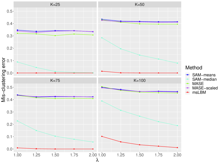
Figure 5.1: Comparison on clustering performance under the setting $1$.

Then, we evaluate the performance of $\widehat{}\mathbf{\Omega}$ and $\{\widehat{}\mathbf{\Theta}_{s}\}_{s\in[m]}$ estimated from msLBM and ASALM. Again, the msLBM performs much better than ASALM. The result is shown in Figure 5.2a and 5.2b. This is intuitive given that msLBM utilizes the information of all views while ASALM doesn’t.

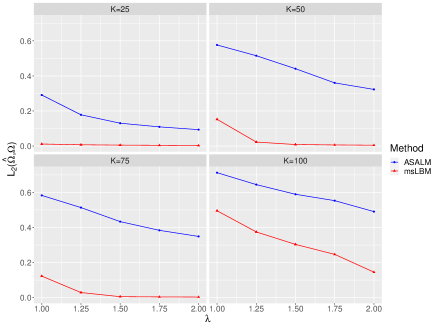
(a) ${\sf L}_{2}(\widehat{\mathbf{\Omega}},\mathbf{\Omega})$

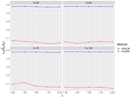
(b) ${\sf L}_{0}(\widehat{\mathbf{\Theta}_{s}},\mathbf{\Theta}_{s})$

Figure 5.2: Comparison on recovering $\mathbf{\Omega}$ and $\mathbf{\Theta}_{s}$ under the setting $1$.

Finally we present the mis-clustering error and the eigenspace of these methods under the setting $2$ in Figure 5.3a and 5.3b, when the three views share a common eigenspace. Even the current models also satisfy the assumption of the completing methods SAM and MASE, msLBM still performs much better than them because it can fully exploit the relative signal and noise strength of each views. On the contrary, SAM can not achieve an optimal weighted combination of all views by simple average. MASE-scaled can use the relative signal strength of each view by using the eigen values of each view. However, it is not robust when the signal strength is small compared to the noise level. So we observe than when $\lambda$ is small, it performs worst. But when $\lambda$ increases, it perform better than MASE. MASE performs worst when $\lambda$ is large because it is totally unweighted.

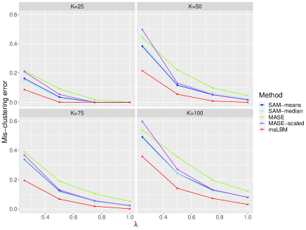
(a) Mis-clustering error

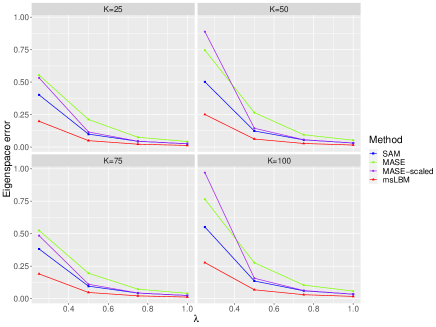
(b) Eigenspace error

Figure 5.3: Comparison on recovering $\mathbf{Z}$ and the eigenspace of $\mathbf{C}$ under the setting $2$.

6 Applications to learning clinical knowledge graph

We next apply the proposed msLBM methods to learn both embeddings for medical concepts and a consensus clinical knowledge graph by synthesizing a few sources of medical text data.

6.1 Data summary

The input data ensemble consists of three similarity matrices of $n=7,217$ clinical concepts, independently derived from three heterogeneous data sources: (i) 10 million clinical narrative notes of 62K patients at Partners Healthcare System (PHS); (ii) 20 million clinical notes from a Stanford hospital [Finlayson et al., 2014]; (iii) clinical notes from the MIMIC-III (Medical Information Mart for Intensive Care) database [Johnson et al., 2016] The clinical concepts were extracted from textual data via natural language processing by mapping clinical terms to Concept Unique Identifiers ($\rm CUI$s) from the Unified Medical Language System (UMLS) [Humphreys and Lindberg, 1993]. Heterogeneity inherently plays a role due to different natures of date sources.

For each source $s$, we construct $\mathbf{W}_{s}$ as the shifted-positive pointwise mutual information (SPPMI) matrix for all $n$ concepts. For a pair of concepts $x$ and $y$, the pointwise mutual information ($\rm PMI$) is a well-known information-theoretic association measure between $x$ and $y$, defined as

$$\rm PMI(x,y)=\log\frac{P(x,y)}{P(x)P(y)}$$

where $P(x,y)$ is the probability of $x$ and $y$ co-occurring and $P(x),P(y)$ are respective marginal occurence probabilities. Using $\rm PMI$ as a measure of association in NLP was introduced by Church and Hanks [1990] and has been widely adopted for word similarity tasks [Dagan et al., 1994, Turney and Pantel, 2010, e.g.]. However, the empirical $\rm PMI$ matrix is not computationally or statistically feasible to use since the PMI estimate would be $-\infty$ for a pair that never co-occurs and the matrix is also dense. The SPPMI matrix with $\rm SPPMI(x,y)=\max\{\widehat{\rm PMI}(x,y),0\}$ is a sparse and consistent alternative estimate of PMI widely used in the NLP literature [Levy and Goldberg, 2014]

We demonstrate below how Algorithm 3 can be used to optimally combine information from the four SPPMI matrices from four data sources to both improve the estimation of embeddings and construct sparse knowledge graph about coronary artery disease network. We aim to group the 7,217 CUIs into $K$ subgroups such that CUIs within the same subgroups are considered synonyms. We anticipate $K$ to be large in this particular application since CUIs were manually curated to represent distinct clinical concepts.

6.2 Clinical concept Embedding and Network

With the three $\rm SPPMI$ matrices as input, our algorithm 3 will output the clinical concept network $\widehat{\mathbf{C}}$. $\widehat{\mathbf{C}}$ has the expression $\widehat{\mathbf{C}}=\widehat{\mathbf{U}}\widehat{\mathbf{U}}^{\top}$ where $\widehat{\mathbf{U}}\in\mathbb{R}^{n\times r}$ is the spherical embedding of the $n$ clinical concepts. We will present that $\widehat{\mathbf{C}}$ (or equivalently $\widehat{\mathbf{U}}$) have better quality than using single source only or other comparable methods.

At first, we can compare the result of our algorithm 3 to the clinical concept learned from single source. Given a $\rm SPPMI$ matrix $\mathbf{W}_{s}$, we can apply our algorithm 4 to it to get the clinical concept network.

In addition, we can compare our method to SAM and MASE. For SAM, we get the $\widehat{\mathbf{V}}_{\textsf{SAM}}\in\mathbb{R}^{n\times r}$ consisting of the leading $r$ eigenvectors of the sum of the three $\rm SPPMI$ matrices. Then we normalize its row to get $\tilde{\mathbf{V}}_{\textsf{SAM}}$, the spherical embedding and the clinical concept network $\widehat{\mathbf{C}}_{\textsf{SAM}}=\tilde{\mathbf{V}}_{\textsf{SAM}}\tilde{\mathbf{V}}_{\textsf{SAM}}^{\top}$. For MASE (or MASE scale), when we get $\widehat{\mathbf{V}}_{\textsf{MASE}}$, we also normalize its rows to get $\tilde{\mathbf{V}}_{\textsf{MASE}}$ and get $\widehat{\mathbf{C}}_{\textsf{MASE}}=\tilde{\mathbf{V}}_{\textsf{MASE}}\tilde{\mathbf{V}}_{\textsf{MASE}}^{\top}$.

We have some parameters to be tuned for our algorithm and for SAM and MASE, we need to tune to rank $r$. To tune the parameters, we use a set of human annotated data. There are two sets of human assessment released by [Pakhomov et al., 2010] on semantic similarity and relatedness between clinical terms. By their definitions, similarity reflects the degree of semantic overlap between words on the level of psycholinguistic definition (e.g., arthritis vs joint pain), while relatedness refers to the probability that one word calls to mind another (e.g., diabetes vs metaformin). We quantify the concordance between human annotation and the learned clinical concept networks based on the rank correlation between human assessment of similarities between CUI pairs and correlation between CUI pairs of the network. These two sets of human annotations serve a great reference to evaluate the quality of the resultant embeddings. Here we use the set of relatedness to tune parameters.

In addition, we can evaluate the quality of the concept networks by its ability of detecting known relation pairs. To be specific, we have five sets of relation pairs of CUIs which are extracted from medical database. They are May Cause (MayCause), May Be Caused By (Causedby), Differential Diagnosis (Ddx), Belong(s) to the Category of (Bco) and May Treat (MayTreat). To be specific, we use the same procedure as Beam et al. [2019] and report the AUC and true positive rate (TPR) with false positive rate (FPR) fixed as 1%, 5% and 10% respectively.

Table 6.1 summarizes the Spearman rank correlation using each single data source and the output given by Algorithm 3 when $r=250$. Table 6.2, 6.3, 6.4 shows the AUC and TPR given FPR = 0.01,0.05,0.1 of relation detection, respectively. Synthesizing information from three data sources via Algorithm 3 yields higher quality embeddings compared to single source concept network as evidenced by the performance of all of these tasks. In addition, our method is obviously better than SAM, MASE and MASE-scaled. In fact, the three methods are even worse than single source in some cases. A possible reason may be that they can not impose suitable weights on different sources.

Method (Data Source)	Relatedness	Similarity
MIMIC	0.533	0.547
Biobank	0.539	0.605
Stanford	0.567	0.660
msLBM	0.635	0.686
SAM	0.588	0.640
MASE	0.577	0.590
MASE-scaled	0.517	0.577

Table 6.1: Spearman rank correlation under $r=250$.

Method (Data Source)	MayCause	Causedby	Ddx	Bco	MayTreat
MIMIC	0.752	0.782	0.789	0.720	0.777
Biobank	0.731	0.764	0.780	0.698	0.787
Stanford	0.757	0.786	0.818	0.741	0.819
msLBM	0.802	0.831	0.864	0.804	0.850
SAM	0.722	0.763	0.770	0.650	0.761
MASE	0.709	0.750	0.773	0.637	0.752
MASE-scaled	0.700	0.739	0.762	0.647	0.751

Table 6.2: AUC of Clinical Relation Detection

Method (Data Source)	MayCause	Causedby	Ddx	Bco	MayTreat
MIMIC	0.339	0.398	0.419	0.238	0.392
Biobank	0.332	0.403	0.399	0.238	0.456
Stanford	0.319	0.385	0.427	0.233	0.465
msLBM	0.429	0.495	0.562	0.374	0.559
SAM	0.371	0.439	0.474	0.239	0.472
MASE	0.333	0.398	0.450	0.205	0.432
MASE-scaled	0.336	0.396	0.448	0.221	0.444

Table 6.3: TPR of Clinical Relation Detection with fixed FPR=0.05

Method (Data Source)	MayCause	Causedby	Ddx	Bco	MayTreat
MIMIC	0.451	0.508	0.523	0.359	0.500
Biobank	0.443	0.511	0.515	0.356	0.558
Stanford	0.458	0.529	0.565	0.420	0.577
msLBM	0.540	0.604	0.672	0.516	0.661
SAM	0.451	0.515	0.542	0.330	0.542
MASE	0.417	0.480	0.538	0.275	0.514
MASE-scaled	0.409	0.473	0.531	0.309	0.514

Table 6.4: TPR of Clinical Relation Detection with fixed FPR=0.1

6.3 Coronary artery disease network

We next construct a disease network Coronary Artery Disease (CAD), a leading causes to deaths involving multiple progression states. We set $K=1000$ and Figure 6.1a suggests the disease network related to CAD is sparse since the magnitude of $\widehat{}\mathbf{\Omega}$ associated with the CAD CUI decays very fast. To further visualize the network, we focused on a subset of 371 CUIs that can have been previously identified from as potentially related to CAD from 5 publicly available knowledge sources – including Mayo, Medline, Medscape, Merck Manuals and Wikipedia–as in Yu et al. [2016]. Algorithm 3 grouped these CUIs into 86 groups. We present in Figures 6.1b the CUIs groups that are most important for CAD as measured by the magnitude of $\widehat{\Omega}_{kl}$ and in  6.1c the CUIs included in each of the CUI groups. Our method is able to yield a very insightful network that unearths the progression states: Hyperlipidemia $\gg$ Atherosclerosis $\gg$ Angina $\gg$ Myocardial Infarction (MI) $\gg$ Congestive Heart Failure (CHF). Associated symptoms such as chest pain are also identified. In addition, our network successfully identifies medications important for CAD including Nitrate: for Angina and Myocardial Infarction; Beta-Blocker for MI and CHF; Anti-platelet for CAD, Angina and MI. In addition to recovering the disease network, our method also successfully grouped near identical concepts into meaningful concept groups as shown in  6.1c. For example the CAD group consists of multiple synonymous concepts including “C0010068” for coronary heart disease, “C0010054” for coronary arteriosclerosis, “C0151744” for myocardial ischemia as well as “C0264694” for chronic myocardial ischemia. All these concepts are frequently used in clinical notes to describe CAD. We observe that CUIs indicative of chest pain have been split into two groups named as “Chest Pain” and “Chest Discomfort” respectively by our method. While it might be ideal from a clinical perspective to merge them together into a single chest pain concept group, such little defect is acceptable due to data quality and more importantly its data-driven nature that will not affect the quality of the overall learned network.

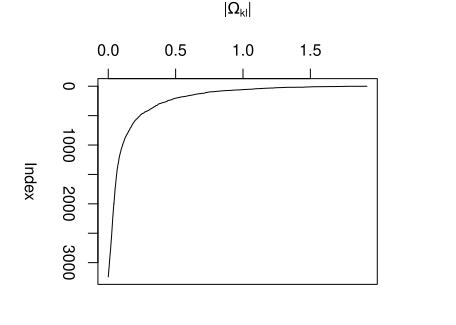
(a) $|\Omega_{kl}|$ decay

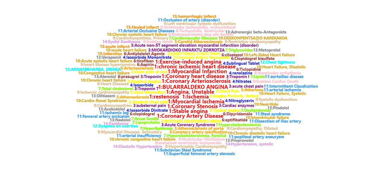
(b) CAD Disease network

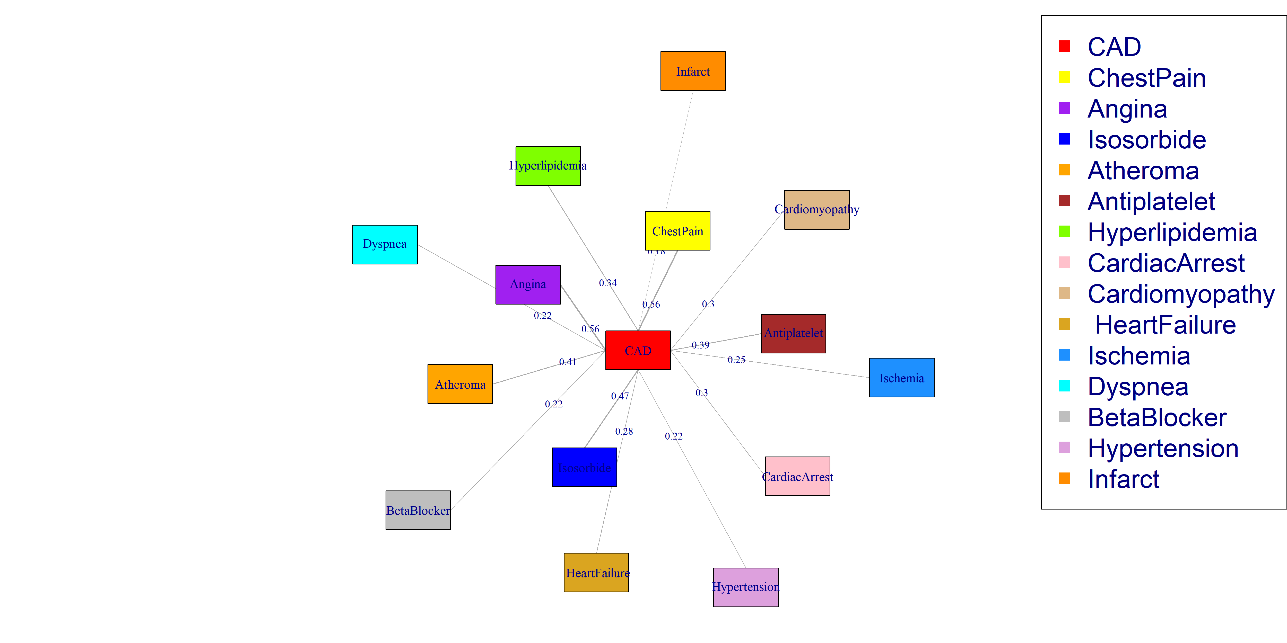
(c) CUIs in different CUI groups

Figure 6.1: Consensus CAD network.

7 Discussion

In this paper, we proposed an msLBM model to synthesize information to learn a consensus graph from multiple sources. Under the msLBM, we developed an alternating minimization algorithm to estimate the unknown parameters associated with the graph and provided convergence properties for the algorithm.

The tuning parameters $\alpha_{s}$, $\lambda_{s}$ and true rank $r$ play crucial roles in the performance of our algorithm. In practice, these parameters are all unknown and need to be estimated from data. The initialization procedure by (3.9) involves a convex optimization which does not rely on the information of the true rank $r$. Empirically, we observe that with properly chosen $\mu$ and $\tau$ (e.g., by cross validation), the solutions $\widehat{}\mathbf{L}_{s}$ and $\widehat{}\mathbf{\Theta}_{s}$ yielded by (3.9) are indeed low-rank and sparse, respectively. We then take the rank of $\widehat{}\mathbf{L}_{s}$ as the value for $r$ and pass it to the Algorithm 3. Meanwhile, the diagonal entries of $\widehat{}\mathbf{L}_{s}$ can be used as the initialization for the heterogeneity matrix $\mathbf{H}_{s}$. We use the $\widehat{\sigma}_{s}^{2}=\|\mathbf{W}_{s}-\widehat{}\mathbf{L}_{s}-\widehat{}\mathbf{\Theta}_{s}\|_{\rm F}^{2}/n^{2}$ as an estimate of $\sigma_{s}^{2}$. Then the tuning parameters are set as $\alpha_{s}=\widehat{h}_{s}^{-4}\widehat{\sigma}_{s}^{-2}$ where $\widehat{h}_{s}$ is the average of the diagonal entries of $\widehat{}\mathbf{L}_{s}$. Finally, the regularization parameter is set at $\lambda_{s}=\alpha_{s}\sigma_{s}\log^{1/2}n$.

References

- Abbe [2018] E. Abbe. Community detection and stochastic block models: Recent developments. Journal of Machine Learning Research, 18(177):1–86, 2018.
- Agency for Healthcare Research and Quality [2019] Agency for Healthcare Research and Quality. Clinical classifications software, 2019. URL http://www.ahcpr.gov/data/hcup/ccs.htm.
- Arroyo et al. [2021] J. Arroyo, A. Athreya, J. Cape, G. Chen, C. E. Priebe, and J. T. Vogelstein. Inference for multiple heterogeneous networks with a common invariant subspace. Journal of Machine Learning Research, 22(142):1–49, 2021.
- Asgari and Mofrad [2015] E. Asgari and M. R. Mofrad. Continuous distributed representation of biological sequences for deep proteomics and genomics. PloS one, 10(11):e0141287, 2015.
- Awasthi et al. [2015] P. Awasthi, M. Charikar, R. Krishnaswamy, and A. K. Sinop. The hardness of approximation of euclidean k-means. arXiv preprint arXiv:1502.03316, 2015.
- Beam et al. [2019] A. L. Beam, B. Kompa, A. Schmaltz, I. Fried, G. Weber, N. Palmer, X. Shi, T. Cai, and I. S. Kohane. Clinical concept embeddings learned from massive sources of multimodal medical data. In PACIFIC SYMPOSIUM ON BIOCOMPUTING 2020, pages 295–306. World Scientific, 2019.
- Bhattacharyya and Chatterjee [2018] S. Bhattacharyya and S. Chatterjee. Spectral clustering for multiple sparse networks: I. arXiv preprint arXiv:1805.10594, 2018.
- Bickel and Chen [2009] P. J. Bickel and A. Chen. A nonparametric view of network models and newman–girvan and other modularities. Proceedings of the National Academy of Sciences, 106(50):21068–21073, 2009.
- Bodenreider [2004] O. Bodenreider. The unified medical language system (UMLS): integrating biomedical terminology. Nucleic acids research, 32(suppl):D267–D270, 2004.
- Cai et al. [2022] J.-F. Cai, J. Li, and D. Xia. Generalized low-rank plus sparse tensor estimation by fast riemannian optimization. Journal of the American Statistical Association, pages 1–17, 2022.
- Candès et al. [2011] E. J. Candès, X. Li, Y. Ma, and J. Wright. Robust principal component analysis? Journal of the ACM (JACM), 58(3):11, 2011.
- Chen et al. [2017] J. Chen, Y. C. Leong, C. J. Honey, C. H. Yong, K. A. Norman, and U. Hasson. Shared memories reveal shared structure in neural activity across individuals. Nature neuroscience, 20(1):115, 2017.
- Choi et al. [2016] Y. Choi, C. Y.-I. Chiu, and D. Sontag. Learning low-dimensional representations of medical concepts. AMIA Summits on Translational Science Proceedings, 2016:41, 2016.
- Church and Hanks [1990] K. W. Church and P. Hanks. Word association norms, mutual information, and lexicography. Computational linguistics, 16(1):22–29, 1990.
- Dagan et al. [1994] I. Dagan, F. Pereira, and L. Lee. Similarity-based estimation of word cooccurrence probabilities. In Proceedings of the 32nd annual meeting on Association for Computational Linguistics, pages 272–278. Association for Computational Linguistics, 1994.
- Finlayson et al. [2014] S. G. Finlayson, P. LePendu, and N. H. Shah. Building the graph of medicine from millions of clinical narratives. Scientific data, 1:140032, 2014.
- Gao et al. [2017] C. Gao, Z. Ma, A. Y. Zhang, and H. H. Zhou. Achieving optimal misclassification proportion in stochastic block models. Journal of Machine Learning Research, 18(1):1980–2024, 2017.
- Goh et al. [2007] K.-I. Goh, M. E. Cusick, D. Valle, B. Childs, M. Vidal, and A.-L. Barabási. The human disease network. Proceedings of the National Academy of Sciences, 104(21):8685–8690, 2007.
- Holland et al. [1983] P. W. Holland, K. B. Laskey, and S. Leinhardt. Stochastic blockmodels: First steps. Social networks, 5(2):109–137, 1983.
- Humphreys and Lindberg [1993] B. L. Humphreys and D. Lindberg. The umls project: making the conceptual connection between users and the information they need. Bulletin of the Medical Library Association, 81(2):170, 1993.
- Jing et al. [2021] B.-Y. Jing, T. Li, Z. Lyu, and D. Xia. Community detection on mixture multilayer networks via regularized tensor decomposition. The Annals of Statistics, 49(6):3181–3205, 2021.
- Johnson et al. [2016] A. E. Johnson, T. J. Pollard, L. Shen, L.-w. H. Lehman, M. Feng, M. Ghassemi, B. Moody, P. Szolovits, L. Anthony Celi, and R. G. Mark. MIMIC-III, a freely accessible critical care database. Scientific Data, 3(1), May 2016. ISSN 2052-4463. doi: 10.1038/sdata.2016.35. URL http://dx.doi.org/10.1038/sdata.2016.35.
- Jones and Rubin-Delanchy [2020] A. Jones and P. Rubin-Delanchy. The multilayer random dot product graph. arXiv preprint arXiv:2007.10455, 2020.
- Karrer and Newman [2011] B. Karrer and M. E. Newman. Stochastic blockmodels and community structure in networks. Physical review E, 83(1):016107, 2011.
- Kelley and Ideker [2005] R. Kelley and T. Ideker. Systematic interpretation of genetic interactions using protein networks. Nature biotechnology, 23(5):561, 2005.
- Kumar et al. [2004] A. Kumar, Y. Sabharwal, and S. Sen. A simple linear time (1+ epsilon)-approximation algorithm for k-means clustering in any dimensions. In Annual Symposium on Foundations of Computer Science, volume 45, pages 454–462. IEEE COMPUTER SOCIETY PRESS, 2004.
- Le et al. [2018] C. M. Le, K. Levin, E. Levina, et al. Estimating a network from multiple noisy realizations. Electronic Journal of Statistics, 12(2):4697–4740, 2018.
- Lei and Rinaldo [2015] J. Lei and A. Rinaldo. Consistency of spectral clustering in stochastic block models. The Annals of Statistics, 43(1):215–237, 2015.
- Lei et al. [2020] J. Lei, K. Chen, and B. Lynch. Consistent community detection in multi-layer network data. Biometrika, 107(1):61–73, 2020.
- Levin et al. [2017] K. Levin, A. Athreya, M. Tang, V. Lyzinski, and C. E. Priebe. A central limit theorem for an omnibus embedding of multiple random dot product graphs. In 2017 IEEE International Conference on Data Mining Workshops (ICDMW), pages 964–967. IEEE, 2017.
- Levin et al. [2022] K. Levin, A. Lodhia, and E. Levina. Recovering shared structure from multiple networks with unknown edge distributions. Journal of Machine Learning Research, 23:3–1, 2022.
- Levy and Goldberg [2014] O. Levy and Y. Goldberg. Neural word embedding as implicit matrix factorization. In Advances in neural information processing systems, pages 2177–2185, 2014.
- Lu et al. [2017] J. Lu, M. Kolar, and H. Liu. Post-regularization inference for time-varying nonparanormal graphical models. The Journal of Machine Learning Research, 18(1):7401–7478, 2017.
- Luscombe et al. [2004] N. M. Luscombe, M. M. Babu, H. Yu, M. Snyder, S. A. Teichmann, and M. Gerstein. Genomic analysis of regulatory network dynamics reveals large topological changes. Nature, 431(7006):308, 2004.
- MacDonald et al. [2022] P. W. MacDonald, E. Levina, and J. Zhu. Latent space models for multiplex networks with shared structure. Biometrika, 109(3):683–706, 2022.
- Mahajan et al. [2009] M. Mahajan, P. Nimbhorkar, and K. Varadarajan. The planar k-means problem is np-hard. In International Workshop on Algorithms and Computation, pages 274–285. Springer, 2009.
- Nabieva et al. [2005] E. Nabieva, K. Jim, A. Agarwal, B. Chazelle, and M. Singh. Whole-proteome prediction of protein function via graph-theoretic analysis of interaction maps. Bioinformatics, 21(suppl_1):i302–i310, 2005.
- Newman [2006] M. E. Newman. Modularity and community structure in networks. Proceedings of the national academy of sciences, 103(23):8577–8582, 2006.
- Ng et al. [2002] A. Y. Ng, M. I. Jordan, and Y. Weiss. On spectral clustering: Analysis and an algorithm. In Advances in neural information processing systems, pages 849–856, 2002.
- Ng [2017] P. Ng. dna2vec: Consistent vector representations of variable-length k-mers. arXiv preprint arXiv:1701.06279, 2017.
- Nguyen et al. [2016] D. Nguyen, W. Luo, D. Phung, and S. Venkatesh. Control matching via discharge code sequences. arXiv preprint arXiv:1612.01812, 2016.
- Nielsen and Witten [2018] A. M. Nielsen and D. Witten. The multiple random dot product graph model. arXiv preprint arXiv:1811.12172, 2018.
- Pakhomov et al. [2010] S. Pakhomov, B. McInnes, T. Adam, Y. Liu, T. Pedersen, and G. B. Melton. Semantic similarity and relatedness between clinical terms: an experimental study. In AMIA annual symposium proceedings, volume 2010, page 572. American Medical Informatics Association, 2010.
- Paul et al. [2020] S. Paul, Y. Chen, et al. Spectral and matrix factorization methods for consistent community detection in multi-layer networks. The Annals of Statistics, 48(1):230–250, 2020.
- Rohe et al. [2011] K. Rohe, S. Chatterjee, B. Yu, et al. Spectral clustering and the high-dimensional stochastic blockmodel. The Annals of Statistics, 39(4):1878–1915, 2011.
- Scott [1988] J. Scott. Social network analysis. Sociology, 22(1):109–127, 1988.
- Shaw et al. [2007] P. Shaw, K. Eckstrand, W. Sharp, J. Blumenthal, J. Lerch, D. Greenstein, L. Clasen, A. Evans, J. Giedd, and J. Rapoport. Attention-deficit/hyperactivity disorder is characterized by a delay in cortical maturation. Proceedings of the National Academy of Sciences, 104(49):19649–19654, 2007.
- Shi and Malik [2000] J. Shi and J. Malik. Normalized cuts and image segmentation. IEEE Transactions on pattern analysis and machine intelligence, 22(8):888–905, 2000.
- Srebro and Jaakkola [2003] N. Srebro and T. Jaakkola. Weighted low-rank approximations. In Proceedings of the 20th International Conference on Machine Learning (ICML-03), pages 720–727, 2003.
- Steinhaus [1956] H. Steinhaus. Sur la division des corp materiels en parties. Bull. Acad. Polon. Sci, 1(804):801, 1956.
- Tang et al. [2017] R. Tang, M. Tang, J. T. Vogelstein, and C. E. Priebe. Robust estimation from multiple graphs under gross error contamination. arXiv preprint arXiv:1707.03487, 2017.
- Tao and Yuan [2011] M. Tao and X. Yuan. Recovering low-rank and sparse components of matrices from incomplete and noisy observations. SIAM Journal on Optimization, 21(1):57–81, 2011.
- Turney and Pantel [2010] P. D. Turney and P. Pantel. From frequency to meaning: Vector space models of semantics. Journal of artificial intelligence research, 37:141–188, 2010.
- Vodrahalli et al. [2018] K. Vodrahalli, P.-H. Chen, Y. Liang, C. Baldassano, J. Chen, E. Yong, C. Honey, U. Hasson, P. Ramadge, K. A. Norman, et al. Mapping between fmri responses to movies and their natural language annotations. Neuroimage, 180:223–231, 2018.
- Wang et al. [2019a] L. Wang, Z. Zhang, and D. Dunson. Common and individual structure of brain networks. The Annals of Applied Statistics, 13(1):85–112, 2019a.
- Wang et al. [2019b] S. Wang, J. Arroyo, J. T. Vogelstein, and C. E. Priebe. Joint embedding of graphs. IEEE transactions on pattern analysis and machine intelligence, 43(4):1324–1336, 2019b.
- Xia et al. [2018] Y. Xia, T. Cai, and T. T. Cai. Multiple testing of submatrices of a precision matrix with applications to identification of between pathway interactions. Journal of the American Statistical Association, 113(521):328–339, 2018.
- Yu et al. [2016] S. Yu, A. Chakrabortty, K. P. Liao, T. Cai, A. N. Ananthakrishnan, V. S. Gainer, S. E. Churchill, P. Szolovits, S. N. Murphy, I. S. Kohane, et al. Surrogate-assisted feature extraction for high-throughput phenotyping. Journal of the American Medical Informatics Association, 24(e1):e143–e149, 2016.
- Zhao et al. [2012] Y. Zhao, E. Levina, J. Zhu, et al. Consistency of community detection in networks under degree-corrected stochastic block models. The Annals of Statistics, 40(4):2266–2292, 2012.
- Zhou and Tao [2011] T. Zhou and D. Tao. Godec: Randomized low-rank & sparse matrix decomposition in noisy case. In International conference on machine learning. Omnipress, 2011.