One-loop calculations for $H\rightarrow f\bar{f}\gamma$ in the $U(1)_{B-L}$ extension for Standard Model

Abstract

In this paper, we present the calculations for $H\rightarrow f\bar{f}\gamma$ in the $U(1)_{B-L}$ extension for Standard Model. Analytic results for one-loop form factors in the decay process are expressed in terms of the scalar one-loop Passarino$-$Veltman functions in the conventions of LoopTools. Therefore, the decay rates can be evaluated numerically by using this package. In phenomenological results, we show the differential decay rates with respect to invariant mass of fermion pair $m_{ff}$, new neutral gauge mass $M_{Z^{\prime}}$ and the coupling $g^{\prime}$ of $U(1)_{B-L}$ gauge group. We find that the contributions of the $U(1)_{B-L}$ extension for Standard Model are visible effects and they must be taken into account at future colliders.

1 Introduction

The precise measurements for the properties of Standard Model like (SM-like) Higgs boson are one of the main targets at the High Luminosity Large Hadron Collider (HL-LHC) [1, 2] and future lepton colliders [3]. It means that all the Higgs productions and decay processes should be probed as accurately as possible. By analyzing these high-precision experimental data, one can verify the Higgs sector for answering the nature of electroweak symmetry breaking (EWSB). It is well-known that many of beyond the Standard Models (BSMs) have extended the Higgs sector as well as gauge sector. As a result, many of BSMs propose new heavy particles such as heavy gauge bosons, heavy fermions as well as heavy scalar particles. The mentioned particles may exchange in the loop of Feynman diagrams in Higgs productions and decay channels. Therefore, the accuracy of the Higgs production cross sections and decay rates are not only used for testing the SM at the high energy regions but also for constraining new parameters in many BSMs. Among Higgs decay channels, the decay processes $H\rightarrow f\bar{f}\gamma$ have been considerable interests recently at the HL-LHC [4, 5, 6, 7].

The computations for one-loop corrections to the decay channel $H\rightarrow f\bar{f}\gamma$ within the SM framework have reported in [11, 12, 13, 14, 15, 16, 17, 18]. While one-loop corrections to $H\rightarrow f\bar{f}\gamma$ in the minimal super-symmetric standard model have computed in [19]. In the current paper, we present the calculations for $H\rightarrow f\bar{f}\gamma$ in the $U(1)_{B-L}$ extension for Standard Model. Analytic results for one-loop form factors in this decay process are expressed in terms of the scalar one-loop Passarino-Veltman functions in the conventions of LoopTools. Therefore, the decay rates can be evaluated numerically by using this package. In phenomenological analyses, we present the differential decay rates with respect the to invariant mass of fermion pair $m_{ff}$, new gauge boson mass $M_{Z^{\prime}}$ and the coupling $g^{\prime}$ of the $U(1)_{B-L}$ gauge group. The contributions of the $U(1)_{B-L}$ extension for Standard Model are visible impacts and these should be taken into account at future colliders. We stress that the detailed of the phenomenological analyses for the decay channel in this model and in the two-Higgs-doublet model can be found in [24].

The outline of this paper is as follows. We review the $U(1)_{B-L}$ extension for Standard Model in section $2$. The evaluations for $H\rightarrow f\bar{f}\gamma$ in this model are also performed in this section. We then present phenomenological results for the decay process in this section. Conclusions and outlooks are shown in the section $3$.

2 Calculation

In this section, we first review the $U(1)_{B-L}$ extension for Standard Model. We then discuss the evaluations for $H\rightarrow f\bar{f}\gamma$ in $U(1)_{B-L}$ extension for standard model.

2.1 Review of the $U(1)_{B-L}$ extension for Standard Model

Reviewing briefly the $U(1)_{B-L}$ extension [20] is presented in this subsection. The model is based on gauge symmetry $SU(3)_{C}\otimes SU(2)_{L}\otimes U(1)_{Y}\otimes U(1)_{B-L}$. In the gauge sector we add new gauge boson $B_{\mu}^{\prime}$ with the coupling $g^{\prime}$. After the spontaneous electroweak symmetry breaking, one has $W^{\pm}$, $Z$ and $Z^{\prime}$ gauge bosons. In the Higgs sector, we include a complex scalar $S$. As a result, general scalar potential is given by

$$V(\Phi,S) = m^{2}\Phi^{{\dagger}}\Phi+\lambda_{1}(\Phi^{{\dagger}}\Phi)^{2}+\mu^{2}|S|^{2}+\lambda_{2}|S|^{4}+\lambda_{3}\Phi^{{\dagger}}\Phi|S|^{2}.$$ (1)

Expanding the scalar fields around their vacuum as follows:

$$\Phi=\begin{pmatrix}\phi^{+}\\ \dfrac{v_{\phi}+h+i\xi}{\sqrt{2}}\end{pmatrix},\quad S=\dfrac{v_{s}+h^{\prime}+i\xi^{\prime}}{\sqrt{2}},$$ (2)

We can observe the mass spectrum of the scalar sector. In detail, the Goldstone bosons $\phi^{\pm},\xi$ will give the masses of $W^{\pm}$ and $Z$ bosons. Working in the unitary gauge, the mass eigenvalues of neutral Higgs are obtained by applying the rotation

$$\begin{pmatrix}h_{1}\\ h_{2}\end{pmatrix}=\begin{pmatrix}c_{\alpha}&-s_{\alpha}\\ s_{\alpha}&c_{\alpha}\\ \end{pmatrix}\begin{pmatrix}h\\ h^{\prime}\end{pmatrix}.$$ (3)

Where the mixing angle is calculated as

$$s_{2\alpha}=\sin 2\alpha=\dfrac{\lambda_{3}v_{\phi}v_{s}}{\sqrt{(\lambda_{1}v_{\phi}^{2}-\lambda_{2}v_{s}^{2})^{2}+(\lambda_{3}v_{\phi}v_{s})^{2}}}.$$ (4)

With the help of the above transformation, we get the masses of scalar Higgs fields as follows:

$$M^{2}_{h_{1}} = \lambda_{1}v_{\phi}^{2}+\lambda_{2}v_{s}^{2}-\sqrt{(\lambda_{1}v_{\phi}^{2}-\lambda_{2}v_{s}^{2})^{2}+(\lambda_{3}v_{\phi}v_{s})^{2}},$$ (5)

$$M^{2}_{h_{2}} = \lambda_{1}v_{\phi}^{2}+\lambda_{2}v_{s}^{2}+\sqrt{(\lambda_{1}v_{\phi}^{2}-\lambda_{2}v_{s}^{2})^{2}+(\lambda_{3}v_{\phi}v_{s})^{2}}.$$ (6)

By expanding the kinematic terms in the scalar sector, we then obtain the masses of gauge bosons $W,Z$ and $Z^{\prime}$. Especially, from the following kinematic terms

$$\mathcal{L}_{\text{K}}\rightarrow(D^{\mu}\Phi)^{+}D_{\mu}\Phi,\quad(D^{\mu}S)^{+}D_{\mu}S.$$ (7)

one has the mass of $Z^{\prime}$ is $M_{Z^{\prime}}=2v_{s}g_{1}^{\prime}$.

In the model, we take into account three right-handed neutrinos. Thus, the Yukawa interaction with including the right-handed neutrinos is expressed as

$$\mathcal{L}_{Y} = -y^{d}_{jk}\bar{q}_{Lj}d_{Rk}\Phi-y^{u}_{jk}\bar{q}_{Lj}u_{Rk}i\sigma_{2}\Phi^{*}-y^{e}_{jk}\bar{l}_{Lj}e_{Rk}\Phi$$ (8)

$$-y^{\nu}_{jk}\bar{l}_{Lj}\nu_{Rk}i\sigma_{2}\Phi^{*}-y^{M}_{jk}\overline{(\nu_{R})}_{j}^{c}\nu_{Rk}\;S+\text{h.c}.$$

for $j,k=1,2,3$. The Majorana mass terms for right-handed neutrinos are corresponding to the last term in above equation. The mass matrix of neutrinos is given after the EWSB

$$M=\begin{pmatrix}0&m_{D}=\dfrac{(y^{\nu})^{*}}{\sqrt{2}}v_{\phi}\\ m_{D}^{T}&\sqrt{2}y^{(M)}\;v_{s}\\ \end{pmatrix}.$$ (9)

The diagonalization is obtained by the transformation

$$\text{diag}\Big{(}-\dfrac{(m^{i}_{D})^{2}}{M^{i}},M^{i}\Big{)}=\begin{pmatrix}\cos\alpha_{i}&-\sin\alpha_{i}\\ \sin\alpha_{i}&\cos\alpha_{i}\\ \end{pmatrix}\begin{pmatrix}0&m_{D}^{i}\\ m_{D}^{i}&M^{i}\\ \end{pmatrix}\begin{pmatrix}\cos\alpha_{i}&\sin\alpha_{i}\\ -\sin\alpha_{i}&\cos\alpha_{i}\\ \end{pmatrix}$$ (10)

for $i=1,2,3$ and $\alpha_{i}=\text{arcsin}(m_{D}^{i}/M^{i})$.

All relevant couplings in the decay under consideration are shown. In the limit of $\alpha_{i}\rightarrow 0$, all the couplings are presented in Table 1

Vertices	Couplings
$h_{1}(h_{2})f\bar{f}$	$-i\dfrac{c_{\alpha}(s_{\alpha})e\;m_{f}}{2M_{W}s_{W}}$
$Z^{\prime}_{\mu}f\bar{f}$	$iQ_{f}\;g^{\prime}_{1}\gamma_{\mu}$
$h_{1}(h_{2})W^{+}_{\mu}W^{-}_{\nu}$	$i\frac{eM_{W}}{s_{W}}\;c_{\alpha}(s_{\alpha})g_{\mu\nu}$
$h_{1}(h_{2})Z_{\mu}Z_{\nu}$	$i\frac{eM_{W}}{c_{W}^{2}\;s_{W}}\;c_{\alpha}(s_{\alpha})g_{\mu\nu}$
$h_{1}(h_{2})Z^{\prime}_{\mu}Z^{\prime}_{\nu}$	$-i4g^{\prime}_{1}M_{Z}^{\prime}\;s_{\alpha}(-c_{\alpha})g_{\mu\nu}$

Table 1: All the couplings involving the decay processes $H\rightarrow f\bar{f}\gamma$ in the $U(1)_{B-L}$ extension of the SM.

2.2 One-loop formulas for $H\rightarrow f\bar{f}\gamma$

General one-loop amplitude for $H\rightarrow f\bar{f}\gamma$ can be decomposed as follows [18]:

$$\mathcal{A}_{\text{loop}} = \sum\limits_{k=1}^{2}\Big{\{}[q_{3}^{\mu}q_{k}^{\nu}-g^{\mu\nu}q_{3}\cdot q_{k}]\bar{u}(q_{1})(F_{k,R}\gamma_{\mu}P_{R}+F_{k,L}\gamma_{\mu}P_{L})v(q_{2})\Big{\}}\varepsilon^{*}_{\nu}(q_{3}).$$ (11)

Where one-loop form factors are computed as follows:

$$F_{k,L/R} = F_{k,L/R}^{\text{$V_{k}^{0*}$-poles}}+F_{k,L/R}^{\text{Non-$V_{k}^{0*}$}}$$ (12)

for $k=1,2$. All related kinematic invariant variables are included: $q^{2}=q_{12}=(q_{1}+q_{2})^{2}$, $q_{13}=(q_{1}+q_{3})^{2}$ and $q_{23}=(q_{2}+q_{3})^{2}$. Here we also used $P_{L/R}=(1\mp\gamma_{5})/2$.

The calculations for this decay process are explained as follows. All one-loop Feynman diagrams for this process in the $U(1)_{B-L}$ extension for Standard Model are shown in [24]. Writing down the amplitudes for all Feynman diagrams in this channel, one then handles Dirac traces and Lorentz contractions in $d$ dimensions with the help of Package-X [21]. As a result, the decay amplitude is then expressed in terms of tensor one-loop integrals. These tensor one-loop integrals can be reduced into scalar one-loop Passarino-Veltman functions (PV-functions)  [22]. The PV-functions are written in the form of LoopTools [23]. As a result, we can perform numerical evaluations for the decay rates by using this program. Analytical results for one-loop form factors are presented in detail in [24]. The decay rates are computed in terms of the one-loop form factors as follows [18]:

$$\dfrac{d\Gamma}{dq_{12}q_{13}}=\dfrac{q_{12}}{512\pi^{3}M_{H}^{3}}\Big{[}q_{13}^{2}(|F_{1,R}|^{2}+|F_{2,R}|^{2})+q_{23}^{2}(|F_{1,L}|^{2}+|F_{2,L}|^{2})\Big{]}.$$ (13)

The integration region is $0\leq q_{12}\leq M_{H}^{2}$ and $0\leq q_{13}\leq M_{H}^{2}-q_{12}$.

2.3 Phenomenological results

We present the phenomenological results for the decay channel in the $U(1)_{B-L}$ extension of the SM. We use the following input parameters for numerical study: $\alpha=1/137.035999084$, $M_{Z}=91.1876$ GeV, $\Gamma_{Z}=2.4952$ GeV, $M_{W}=80.379$ GeV, $M_{H}=125.1$ GeV, $m_{\tau}=1.77686$ GeV, $m_{t}=172.76$ GeV, $m_{b}=4.18$ GeV, $m_{s}=0.93$ GeV and $m_{c}=1.27$ GeV. We include three more parameters such as the coupling $g^{\prime}$, boson mass $M_{Z^{\prime}}$ and the mixing angle $\alpha$ (or $c_{\alpha},s_{\alpha}$).

In the Fig. 1, differential decay rates with respect to $g^{\prime}$ for $M_{Z^{\prime}}=800$ GeV (left panel) and for $M_{Z^{\prime}}=1000$ GeV (right panel) are shown. In both Figures, we fix the mixing angle $c_{\alpha}=0.5$. We find that the decay rates are proportional to $g^{\prime}$. Furthermore, one can verify that decay rates are inversely proportional to $M_{Z^{\prime}}$.

$\begin{array}[]{cc}d\Gamma/dg^{\prime}[\textrm{GeV}]&d\Gamma/dg^{\prime}[\textrm{GeV}]\\ \includegraphics[width=219.08612pt,height=213.39566pt]{HFFG_U1_gBL_05_MZ1000.eps}&\includegraphics[width=219.08612pt,height=213.39566pt]{HFFG_U1_gBL_08_MZ1000.eps}\\ \hskip 199.16928ptg^{\prime}&\hskip 199.16928ptg^{\prime}\end{array}$

Figure 1: Differential decay rates with respect to $g^{\prime}$ for $M_{Z^{\prime}}=800$ GeV (left panel) and for $M_{Z^{\prime}}=1000$ GeV (right panel).

In the Fig. 2, differential decay rates with respect to the invariant mass of fermion pair $m_{ff}$ (left panel) and $M_{Z^{\prime}}$ (right panel) are plotted. In the left Figure, the solid line shows for the case of $c_{\alpha}=1$ (it is also corresponding to the SM case), the dashed line presents for the case of $c_{\alpha}=0.8$ and the dotted line is for for the case of $c_{\alpha}=0.5$, respectively. In the right Figure, we select the values of $c_{\alpha}=0.3,0.5,0.8$ and change $M_{Z^{\prime}}$ from $800$ GeV to $1500$ GeV. In this Figure, the dashed line presents for the case of $c_{\alpha}=0.3$, the dotted line is for the case of $c_{\alpha}=0.5$ and the dotted dashed line is for the case of $c_{\alpha}=0.8$. One observes the peak of the decay rates at $m_{ff}=M_{Z}=91.1876$ GeV which is corresponding to the resonance of $Z\rightarrow f\bar{f}$. We find that the decay rates are inversely proportional to the $M_{Z^{\prime}}$. It is interested to observe that the contributions from the $U(1)_{B-L}$ extension of the SM are visible impacts. These effects must be taken into account at future colliders.

$\begin{array}[]{cc}d\Gamma/dm_{ff}[\textrm{GeV}]&d\Gamma/dM_{Z^{\prime}}[\textrm{GeV}]\\ \includegraphics[width=219.08612pt,height=213.39566pt]{HFFG_U1_mll.eps}&\includegraphics[width=219.08612pt,height=210.55022pt]{HFFG_U1_MZBL.eps}\\ \hskip 170.71652ptm_{ff}[\textrm{GeV}]&\hskip 170.71652ptm_{Z^{\prime}}[\textrm{GeV}]\end{array}$

Figure 2: Differential decay rates with respect to the invariant mass of fermion pair $m_{ff}$ (left panel) and $M_{Z^{\prime}}$ (right panel).

In the Fig. 3, differential decay rates with respect to $M_{Z^{\prime}}$ and $g^{\prime}$ are shown. We vary the coupling $0.01\leq g^{\prime}\leq 0.5$ and boson mass $600$ GeV $\leq M_{Z^{\prime}}\leq 1500$ GeV. We have the same conclusions as previous cases that the decay rates are proportional to $g^{\prime}$ and inversely proportional to the $M_{Z^{\prime}}$. Full analyses for the decay channel in this model and in the two-Higgs-doublet model can be found in [24].

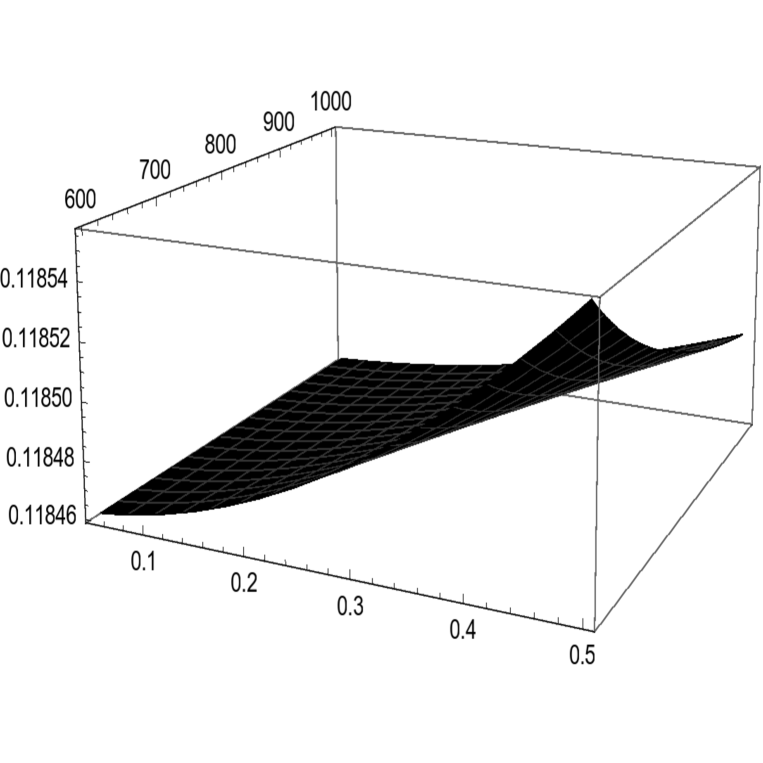
Figure 3: Differential decay rates with respect to $M_{Z^{\prime}}$ and $g^{\prime}$.

3 Conclusions

In the current paper, we have presented the calculations for $H\rightarrow f\bar{f}\gamma$ in the $U(1)_{B-L}$ extension for Standard Model. Analytic results for one-loop form factors in this decay process are expressed in terms of the scalar one-loop Passarino-Veltman functions in the conventions of LoopTools. Therefore, the decay rates can be evaluated numerically by using this package. In phenomenological results, we have shown differential decay rates with respect to $m_{ff}$, $M_{Z^{\prime}}$ and $g^{\prime}$. We find that the contributions of the $U(1)_{B-L}$ extension for Standard Model are visible effects and they must be taken into account at future colliders.

Acknowledgment:  This research is funded by Vietnam National University, Ho Chi Minh City (VNU-HCM) under grant number C$2022$-$18$-$14$.

References

References

• [1] Liss A et al. [ATLAS] 2013 [arXiv:1307.7292 [hep-ex]]
• [2] [CMS] Collaboration 2013 [arXiv:1307.7135 [hep-ex]]
• [3] Baer H, Barklow T, Fujii K, Gao Y, Hoang A, Kanemura S, et al. 2013
• [4] Khachatryan V et al. [CMS] 2016 Phys. Lett. B 753 341-362
• [5] Sirunyan A et al. [CMS] 2018 JHEP 09 148
• [6] Sirunyan A et al. [CMS] 2018 JHEP 11 152
• [7] Aad G et al. [ATLAS] 2021 Phys. Lett. B 819 136412
• [8] Chen L, Qiao C and Zhu R 2013 Phys. Lett. B 726 306-311
• [9] Gainer J, Keung W, Low I and Schwaller P 2012 Phys. Rev. D 86 033010
• [10] Korchin A and Kovalchuk V 2014 Eur. Phys. J. C 74 no.11, 3141
• [11] Abbasabadi A, Bowser-Chao D, Dicus D and Repko W 1995 Phys. Rev. D 52 3919-3928.
• [12] Djouadi A, Driesen V, Hollik W and Rosiek J 1997 Nucl. Phys. B 491 68-102
• [13] Abbasabadi A and Repko W 2000 Phys. Rev. D 62 054025
• [14] Dicus D and Repko W 2013 Phys. Rev. D 87 no.7, 077301
• [15] Sun Y, Chang H and Gao D 2013 JHEP 05 061
• [16] Passarino G 2013 Phys. Lett. B 727 424-431
• [17] Dicus D, Kao C and Repko W 2014 Phys. Rev. D 89 no.3, 033013
• [18] Kachanovich A, Nierste U and NiΕ‘andΕΎiΔ‡ I 2020 Phys. Rev. D 101 no.7, 073003
• [19] Li C, Qiao C and Zhu S 1998 Phys. Rev. D 57 6928-6933
• [20] Basso L, Belyaev A, Moretti S and Shepherd-Themistocleous C 2009 Phys. Rev. D 80 055030
• [21] Patel H 2015 Comput. Phys. Commun. 197 276-290
• [22] Denner A and Dittmaier S 2006 Nucl. Phys. B 734 62-115
• [23] Hahn T and Perez-Victoria M 1999 Comput. Phys. Commun. 118 153-165
• [24] On V, Tran D, Nguyen C and Phan K, 2022 Eur. Phys. J. C 82 (2022)