Inspiral gravitational waveforms from compact binary systems in Horndeski gravity

Abstract

In a subclass of Horndeski theories with the speed of gravity equivalent to that of light, we study gravitational radiation emitted during the inspiral phase of compact binary systems. We compute the waveform of scalar perturbations under a post-Newtonian expansion of energy-momentum tensors of point-like particles that depend on a scalar field. This scalar mode not only gives rise to breathing and longitudinal polarizations of gravitational waves, but it is also responsible for scalar gravitational radiation in addition to energy loss associated with transverse and traceless tensor polarizations. We calculate the Fourier-transformed gravitational waveform of two tensor polarizations under a stationary phase approximation and show that the resulting waveform reduces to the one in a parametrized post-Einsteinian (ppE) formalism. The ppE parameters are directly related to a scalar charge in the Einstein frame, whose existence is crucial to allow the deviation from General Relativity (GR). We apply our general framework to several concrete theories and show that a new theory of spontaneous scalarization with a higher-order scalar kinetic term leaves interesting deviations from GR that can be probed by the observations of gravitational waves emitted from neutron star-black hole binaries. If the scalar mass exceeds the order of typical orbital frequencies $\omega\simeq 10^{-13}$ eV, which is the case for a recently proposed scalarized neutron star with a self-interacting potential, the gravitational waveform practically reduces to that in GR.

I Introduction

The discovery of gravitational waves (GWs) Abbott et al. (2016) opened up a new window for probing the physics in strong gravity regimes Berti et al. (2015); Barack et al. (2019); Berti et al. (2018). Up to now, there have been many observed events of the coalescence of two black holes (BHs) Abbott et al. (2019, 2021). The merger of two neutron stars (NSs) was first detected as the event GW170817 Abbott et al. (2017a), together with an electromagnetic counterpart Goldstein et al. (2017). This latter event constrained the speed of gravity to be very close to that of light Abbott et al. (2017b). There was also a possible NS-BH coalescence event GW190426-152155, albeit its highest false alarm rate Abbott et al. (2020); Broekgaarden et al. (2021); Li et al. (2020); Niu et al. (2021). The increasing sensitivity in future GW observations will allow one to detect more promising events of the NS-BH coalescence.

General Relativity (GR) is a fundamental theory of gravity consistent with submillimeter laboratory tests Hoyle et al. (2001); Adelberger et al. (2003), solar system constraints Will (2014), and binary pulsar measurements Taylor and Weisberg (1982); Stairs (2003); Antoniadis et al. (2013). However, there are several cosmological problems like the origins of inflation, dark energy, and dark matter, which are difficult to be resolved within the framework of GR and standard model of particle physics Lyth and Riotto (1999); Copeland et al. (2006); Bertone et al. (2005). To address these problems, one usually introduces additional degrees of freedom beyond those appearing in GR (two tensor polarizations). The simplest example is a scalar field $\phi$ minimally or nonminimally coupled to gravity. If there is a nonminimal coupling with the Ricci scalar $R$ of the form $F(\phi)R$, the gravitational interaction is generally modified from that in GR. Brans-Dicke (BD) theories Brans and Dicke (1961) with a scalar potential $V(\phi)$ belong to such a class, which accommodates $f(R)$ gravity Starobinsky (1980) as a special case. The applications of BD theories and $f(R)$ gravity to inflation and dark energy have been extensively performed in the literature (see the reviews Sotiriou and Faraoni (2010); De Felice and Tsujikawa (2010)).

In BD theories, the NS can have a scalar hair through the coupling between the scalar field and matter mediated by gravity. On the other hand, the no-hair property of BHs was proven in BD theories Hawking (1972); Bekenstein (1995); Sotiriou and Faraoni (2012). This means that the binary system containing at least one scalarized NS may leave some signatures for the deviation from GR in inspiral gravitational waveforms. In massless BD theories, Eardley Eardley (1975) estimated the change of an orbital period induced by dipole gravitational radiation in a compact binary system. In the same theories, Will Will (1994) computed gravitational waveforms radiated during an inspiral phase of the compact binary up to the Newtonian quadrupole order (see also Refs. Shibata et al. (1994); Harada et al. (1997); Brunetti et al. (1999); Berti et al. (2005); Scharre and Will (2002); Chatziioannou et al. (2012) for related works). Under a so-called post-Newtonian (PN) approximation Blanchet (2014) based on slow velocities of the binary system relative to the speed of light $c$, the gravitational radiation was also calculated up to 2PN Lang (2014); Mirshekari and Will (2013); Lang (2015); Sennett et al. (2016) and 2.5PN Bernard et al. (2022) orders, with the equations of motion up to 3PN order Bernard (2018).

In massless BD theories given by the Lagrangian $L=(1/2)\phi R+\omega_{\rm BD}X/\phi$, where $X=-(1/2)\nabla^{\mu}\phi\nabla_{\mu}\phi$ is a field kinetic term with the covariant derivative operator $\nabla^{\mu}$, the solar-system tests of gravity put a tight bound on the BD parameter, $\omega_{\rm BD}>4.0\times 10^{4}$ Will (2014). With this constraint, the deviation from GR in strong gravity regimes is limited to be small. In other words, the GW measurements need to reach high sensitivities to distinguish between BD theories and GR from the observed gravitational waveform. If the scalar field has a potential $V(\phi)$ with a heavy mass inside a nonrelativistic star, while having a light mass outside the star, it is possible to suppress the propagation of fifth forces in the solar system through a so-called chameleon mechanism Khoury and Weltman (2004a, b). In such cases the constraint on $\omega_{\rm BD}$ is loosened Faulkner et al. (2007); Hu and Sawicki (2007); Capozziello and Tsujikawa (2008); Tsujikawa et al. (2008); Berti et al. (2012), so there is more freedom to probe signatures of the modification of gravity in strong gravity environments. The gravitational radiation and tensor waves emitted from a compact binary have been computed in massive BD theories Alsing et al. (2012); Berti et al. (2012); Sagunski et al. (2018); Liu et al. (2020) and screened modified gravity in the Einstein frame Zhang et al. (2017); Liu et al. (2018); Niu et al. (2019).

In the presence of a nonminimal coupling of the form $F(\phi)R$, there is yet the other scenario dubbed spontaneous scalarization of NSs Damour and Esposito-Farese (1993, 1996) in which the modification of gravity manifests itself only on the strong gravity background. Provided that $F(\phi)$ contains even power-law functions of $\phi$, the theory admits the existence of a nonvanishing field branch besides the GR branch ($\phi=0$). Since the Ricci scalar $R$ coupled to the scalar field is large inside the NS, the GR branch can be unstable to trigger tachyonic growth of $\phi$ toward the other nontrivial branch. For the nonminimal coupling $F(\phi)=e^{-\beta\phi^{2}/(2M_{\rm Pl}^{2})}$ chosen by Damour and Esposito-Farese Damour and Esposito-Farese (1993), spontaneous scalarization can occur for the coupling constant $\beta\leq-4.35$ Harada (1998); Novak (1998); Sotani and Kokkotas (2004); Silva et al. (2015); Barausse et al. (2013). On the other hand, the presence of a scalar charge for the scalarized solution leads to an energy loss through dipolar gravitational radiation. This results in time variation of the orbital period of binary systems. Indeed, binary-pulsar observations put the bound $\beta\geq-4.5$ Freire et al. (2012); Shao et al. (2017); Anderson et al. (2019), so the coupling constant $\beta$ is confined in a limited range. Since the gravitational waveform emitted from compact binaries containing a NS should give an independent constraint on the scalar charge, it remains to be seen how the future GW observations place the bound on $\beta$. In Ref. Niu et al. (2021), the authors started to derive constraints on $\beta$ by using the possible NS-BH coalescence event GW190426-152155.

Theory of spontaneous scalarization does not belong to a framework of BD theories, but it can be accommodated as a generalized class of BD theories by promoting the BD parameter $\omega_{\rm BD}$ to a scalar-field dependent function $\omega(\phi)$. Indeed, the gravitational radiation and waveforms in theories given by the Lagrangian $L=(1/2)\phi R+\omega(\phi)X/\phi$ have been investigated in Refs. Alsing et al. (2012); Yunes et al. (2012); Berti et al. (2018); Liu et al. (2020). Such theories belong to a scheme of Horndeski theories Horndeski (1974)– most general scalar-tensor theories with second-order Euler-Lagrange equations of motion Deffayet et al. (2011); Kobayashi et al. (2011); Charmousis et al. (2012). The subclass of Horndeski theories with the speed of gravity equivalent to that of light is given by the Lagrangian $L=G_{2}(\phi,X)-G_{3}(\phi,X)\square\phi+G_{4}(\phi)R$ Kobayashi et al. (2011); De Felice and Tsujikawa (2012); Kase and Tsujikawa (2019), where $G_{2}$ and $G_{3}$ are functions of $\phi$ and $X$, and $G_{4}$ is a function of $\phi$. This class of theories automatically evades the observational bound on the speed of gravity constrained by the GW170817 event Abbott et al. (2017b).

Theories with the Lagrangian $L=G_{2}(\phi,X)+G_{4}(\phi)R$ accommodate not only the generalized massive BD theories with $L=(1/2)\phi R+\omega(\phi)X/\phi-V(\phi)$ but also nonminimally coupled k-essence Armendariz-Picon et al. (1999); Chiba et al. (2000); Armendariz-Picon et al. (2000); Arkani-Hamed et al. (2004); Piazza and Tsujikawa (2004); ter Haar et al. (2021); Bezares et al. (2022) containing higher-order kinetic terms like $\mu_{2}X^{2}$ in $G_{2}$. When spontaneous scalarization occurs inside the NS, higher-order derivatives can be as large as the linear kinetic term around the surface of star. Indeed, we will propose a new scenario of spontaneous scalarization where the scalar charge is reduced by an additional term $\mu_{2}X^{2}$. This allows a possibility for alleviating the tension of the coupling constant $\beta$ mentioned above. The modified scalar-field solution also affects the gravitational waveform radiated from the binary system containing a NS. Thus, it is convenient to provide a general scheme for confronting such theories with future GW observations of the NS-BH or NS-NS coalescence.

In this paper, we compute the gravitational waveform emitted during the inspiral phase of compact binary systems in a subclass of Horndeski theories given by the Lagrangian $L=G_{2}(\phi,X)-G_{3}(\phi,X)\square\phi+G_{4}(\phi)R$. For this purpose, we perform the PN expansion of a source energy-momentum tensor and neglect nonlinear derivative terms arising from the cubic coupling $G_{3}(X)\square\phi$ outside the source. This amounts to neglecting nonlinear Galileon-type self-interactions Nicolis et al. (2009); Deffayet et al. (2009) relative to the linear kinetic term. Hence it is difficult to accommodate the case in which the field derivative is suppressed in the exterior region of NSs by the Vainshtein mechanism Vainshtein (1972); Burrage and Seery (2010); De Felice et al. (2012); Kimura et al. (2012); Koyama et al. (2013), unless some specific scaling methods McManus et al. (2016); Renevey et al. (2020, 2022) are employed. However, if the Vainshtein radius $r_{V}$ is of the same order as the NS radius $r_{s}$ ($\sim 10$ km), the PN analysis used for the derivation of solutions to scalar perturbations from $r=r_{s}$ to an observer does not lose its validity. In such a case, the field derivative and scalar charge can be suppressed by the Vainshtein screening inside the NS, analogous to the findings in Ref. Chagoya et al. (2014); Ogawa et al. (2020). Thus, the gravitational waveform derived in this paper can be applied to the case $r_{V}\lesssim r_{s}$.

This paper is organized as follows. In Sec. II, we review the field equations of motion and the matter action of two point-like sources in the subclass of Horndeski theories. In Sec. III, we perform the weak-field expansions of metric and scalar field to study the propagation of GWs from the binary system of a quasicircular orbit to the observer and derive solutions to tensor GWs. In Sec. IV, we obtain the time-domain gravitational waveforms corresponding to two transverse and longitudinal tensor polarizations as well as breathing and longitudinal modes. In Sec. V, we study the energy loss induced by the GW emission and derive the Fourier-transformed gravitational waveforms by using a stationary phase approximation. We show that the resulting waveform reduces to the one in a parameterized post-Einsteinian (ppE) framework Yunes and Pretorius (2009); Cornish et al. (2011); Chatziioannou et al. (2012); Tahura and Yagi (2018) and derive the ppE parameters in our theory. In Sec. VI, we apply our general results to several concrete theories and clarify the relations between ppE parameters and the scalar charge in the Einstein frame. In particular, we show that a new theory of spontaneous scalarization with the higher-order derivative term $\mu_{2}X^{2}$ in $G_{2}$ allows an interesting possibility for reducing the scalar charge in comparison to the case $\mu_{2}=0$, whose property can be probed in future GW observations. Sec. VII is devoted conclusions.

Throughout the paper, we use the metric signature $(-,+,+,+)$ and natural units $c=\hbar=1$, where $\hbar$ is the reduced Planck constant.

II Subclass of Horndeski theories and field equations of motion

We consider a subclass of Horndeski theories Horndeski (1974) given by the action

$${\cal S}=\int{\rm d}^{4}x\sqrt{-g}\left[G_{2}(\phi,X)-G_{3}(\phi,X)\square\phi+G_{4}(\phi)R\right]+{\cal S}_{m}(g_{\mu\nu},\Psi_{m})\,,$$ (1)

where $g$ is the determinant of metric tensor $g_{\mu\nu}$, $X=-(1/2)\nabla^{\mu}\phi\nabla_{\mu}\phi$ is the kinetic term of a scalar field $\phi$, and $\square\equiv g^{\mu\nu}\nabla_{\mu}\nabla_{\nu}$ is the d’Alembertian. The action ${\cal S}_{m}$ contains matter fields $\Psi_{m}$ minimally coupled to gravity. In theories (1), there are no asymptotically flat spherically symmetric and static BH solutions with a scalar hair Hawking (1972); Bekenstein (1995); Sotiriou and Faraoni (2012); Graham and Jha (2014); Faraoni (2017); Minamitsuji et al. (2022). On the other hand, NSs can have scalar charges in the presence of nonminimal couplings $G_{4}(\phi)R$ Eardley (1975).

Our aim is to compute a gravitational waveform emitted from inspiraling compact binaries containing at least one NS. If the NS has a scalar hair, the waveform is subject to modifications in comparison to GR. This allows us to probe signatures for the possible existence of a scalar field nonminimally coupled to gravity. In theories given by the action (1), the speed of gravity on the cosmological background is identical to that of light Kobayashi et al. (2011); De Felice and Tsujikawa (2012); Kase and Tsujikawa (2019). We note that the equivalence principle can be generally violated in scalar-tensor theories including the action (1). However, in concrete models discussed in Sec. VI, we are interested in the case where the fifth force induced by scalar-gravitational couplings is suppressed on weak gravity backgrounds for the consistency with solar-system constraints. For the derivation of gravitational waveforms, we do not restrict the analysis to some specific models by the end of Sec. V.

We deal with the binary system of a quasicircular orbit as a collection of two point-like particles with masses $m_{I}(\phi)$, where $I=A,B$ for each particle. Since the existence of $\phi$ affects matter through gravitational field equations of motion, there is the $\phi$-dependence in $m_{I}$. The matter sector is expressed by the action Eardley (1975)

$${\cal S}_{m}=-\sum_{I=A,B}\int m_{I}(\phi){\rm d}\tau_{I}\,,$$ (2)

where $\tau_{I}$ is the proper time along the world line $x_{I}^{\mu}$ of particle $I$. The infinitesimal line element is given by

$${\rm d}s^{2}=-{\rm d}\tau^{2}=g_{\mu\nu}{\rm d}x^{\mu}{\rm d}x^{\nu}\,.$$ (3)

Then, the matter action (2) can be written as

$${\cal S}_{m}=-\sum_{I=A,B}\int{\rm d}^{4}x\,m_{I}(\phi)\sqrt{-g_{\mu\nu}{\rm d}x_{I}^{\mu}{\rm d}x_{I}^{\nu}}\,\delta^{(4)}(x^{\mu}-x_{I}^{\mu})\,,$$ (4)

where $\delta^{(4)}(x^{\mu}-x_{I}^{\mu})$ is the four dimensional delta function. Varying (4) with respect to $g_{\mu\nu}$, it follows that

$$\frac{\delta{\cal S}_{m}}{\delta g_{\mu\nu}}=\sum_{I=A,B}\frac{1}{2}\int{\rm d}^{4}x\,\int{\rm d}\tau_{I}\,m_{I}(\phi)u_{I}^{\mu}u_{I}^{\nu}\,\delta^{(4)}(x^{\mu}-x_{I}^{\mu})\,,$$ (5)

where $u_{I}^{\mu}={\rm d}x_{I}^{\mu}/{\rm d}\tau_{I}$ is the four velocity of particle $I$. The matter energy-momentum tensor $T^{\mu\nu}$ is defined by

$$\delta{\cal S}_{m}=\frac{1}{2}\int{\rm d}^{4}x\sqrt{-g}\,T^{\mu\nu}\delta g_{\mu\nu}\,.$$ (6)

Comparing Eq. (6) with Eq. (5), we obtain

$$T^{\mu\nu} = \frac{1}{\sqrt{-g}}\sum_{I=A,B}\int{\rm d}\tau_{I}\,m_{I}(\phi)u_{I}^{\mu}u_{I}^{\nu}\delta^{(4)}(x^{\mu}-x_{I}^{\mu})$$ (7)

$$= \frac{1}{\sqrt{-g}}\sum_{I=A,B}m_{I}(\phi)\frac{u_{I}^{\mu}u_{I}^{\nu}}{u_{I}^{0}}\delta^{(3)}({\bm{x}}-{\bm{x}}_{I}(t))\,.$$ (8)

In the second line, we used ${\rm d}\tau_{I}={\rm d}x_{I}^{0}/u_{I}^{0}$ and integrated Eq. (7) with respect to $x_{I}^{0}$. Note that $\delta^{(3)}({\bm{x}}-{\bm{x}}_{I}(t))$ is a three dimensional delta function and that the time $t$ is determined by $t=x_{I}^{0}$.

On using the property $g_{\mu\nu}u_{I}^{\mu}u_{I}^{\nu}=-1$, the trace of Eq. (8) yields

$$T\equiv g_{\mu\nu}T^{\mu\nu}=-\frac{1}{\sqrt{-g}}\sum_{I=A,B}m_{I}(\phi)\frac{1}{u_{I}^{0}}\delta^{(3)}({\bm{x}}-{\bm{x}}_{I}(t))\,.$$ (9)

On the other hand, the action (2) can be written in the form

$${\cal S}_{m}=-\sum_{I=A,B}\int{\rm d}^{4}x\,m_{I}(\phi)\frac{1}{u_{I}^{0}}\delta^{(3)}({\bm{x}}-{\bm{x}}_{I}(t))\,.$$ (10)

Comparing Eq. (9) with Eq. (10), it follows that

$${\cal S}_{m}=\int{\rm d}^{4}x\sqrt{-g}\,T(\phi)\,,$$ (11)

whose form is used for the variation of ${\cal S}_{m}$ with respect to $\phi$.

Varying the action (1) with respect to $g^{\mu\nu}$, we obtain the covariant gravitational field equations of motion Kobayashi et al. (2011)

$$-G_{2,X}\nabla_{\mu}\phi\nabla_{\nu}\phi-G_{2}g_{\mu\nu}+G_{3,X}\square\phi\nabla_{\mu}\phi\nabla_{\nu}\phi+\nabla_{\mu}G_{3}\nabla_{\nu}\phi+\nabla_{\nu}G_{3}\nabla_{\mu}\phi-g_{\mu\nu}\nabla^{\lambda}G_{3}\nabla_{\lambda}\phi$$

$$+2G_{4}G_{\mu\nu}+2g_{\mu\nu}\left(G_{4,\phi}\square\phi-2XG_{4,\phi\phi}\right)-2G_{4,\phi}\nabla_{\mu}\nabla_{\nu}\phi-2G_{4,\phi\phi}\nabla_{\mu}\phi\nabla_{\nu}\phi=T_{\mu\nu}\,,$$ (12)

where we used the notations like $G_{2,X}=\partial G_{2}/\partial X$, $G_{4,\phi\phi}=\partial^{2}G_{4}/\partial\phi^{2}$, etc. The variation of (1) with respect to $\phi$ leads to the scalar-field equation of motion

$$\nabla^{\mu}J_{\mu}={\cal P}_{\phi}\,,$$ (13)

where

$$J_{\mu} = -G_{2,X}\nabla_{\mu}\phi+G_{3,X}\square\phi\nabla_{\mu}\phi+G_{3,X}\nabla_{\mu}X+2G_{3,\phi}\nabla_{\mu}\phi\,,$$ (14)

$${\cal P}_{\phi} = G_{2,\phi}+\nabla^{\mu}G_{3,\phi}\nabla_{\mu}\phi+G_{4,\phi}R+T_{,\phi}\,.$$ (15)

The $\phi$ dependence in $T(\phi)$ influences the scalar-field equation through the last term in Eq. (15). The Ricci scalar $R$ in ${\cal P}_{\phi}$ is affected by the presence of matter through the gravitational Eq. (12). Taking the trace of Eq. (12), we obtain

$$2G_{4}R=2XG_{2,X}-4G_{2}-2XG_{3,X}\square\phi-2\nabla^{\mu}G_{3}\nabla_{\mu}\phi+6\left(G_{4,\phi}\square\phi-2XG_{4,\phi\phi}\right)-T\,.$$ (16)

Then, we can express ${\cal P}_{\phi}$ in the following form

$${\cal P}_{\phi} = G_{2,\phi}+\nabla^{\mu}G_{3,\phi}\nabla_{\mu}\phi+\frac{G_{4,\phi}}{G_{4}}\left(XG_{2,X}-2G_{2}-XG_{3,X}\square\phi-\nabla^{\mu}G_{3}\nabla_{\mu}\phi+3G_{4,\phi}\square\phi-6XG_{4,\phi\phi}\right)$$ (17)

$$+T_{,\phi}-\frac{G_{4,\phi}}{2G_{4}}T\,.$$

The last two contributions to Eq. (17) work as matter source terms for the scalar-field equation.

The matter action (2) can be also expressed in the form

$${\cal S}_{m}=-\sum_{I=A,B}\int m_{I}(\phi(x_{I}^{\lambda}))\sqrt{-g_{\mu\nu}(x_{I}^{\lambda})u_{I}^{\mu}u_{I}^{\nu}}\,{\rm d}\tau_{I}\,.$$ (18)

Varying this action with respect to $x_{I}^{\lambda}$ and integrating it by parts, we obtain

$$\delta{\cal S}_{m}=-\sum_{I=A,B}\int\left[\frac{{\rm d}}{{\rm d}\tau}\left(m_{I}g_{\mu\lambda}u_{I}^{\mu}\right)-\frac{1}{2}m_{I}\frac{\partial g_{\mu\nu}}{\partial x_{I}^{\lambda}}u_{I}^{\mu}u_{I}^{\nu}+m_{I,\phi}\frac{\partial\phi}{\partial x_{I}^{\lambda}}\right]\delta x_{I}^{\lambda}{\rm d}\tau\,.$$ (19)

Then, the equation of motion for the $I$-th particle is given by

$$\frac{{\rm d}}{{\rm d}\tau}\left(m_{I}g_{\mu\lambda}u_{I}^{\mu}\right)-\frac{1}{2}m_{I}\frac{\partial g_{\mu\nu}}{\partial x_{I}^{\lambda}}u_{I}^{\mu}u_{I}^{\nu}+m_{I,\phi}\frac{\partial\phi}{\partial x_{I}^{\lambda}}=0\,.$$ (20)

Multiplying Eq. (20) by $g^{\alpha\lambda}$ and using ${\rm d}m_{I}/{\rm d}\tau=m_{I,\phi}u^{\beta}\nabla_{\beta}\phi$ and ${\rm d}g_{\mu\lambda}/{\rm d}\tau=(\partial g_{\mu\lambda}/\partial x_{I}^{\nu})u_{I}^{\nu}/2+(\partial g_{\lambda\mu}/\partial x_{I}^{\nu})u_{I}^{\nu}/2$, it follows that

$$m_{I}\left(\frac{{\rm d}u_{I}^{\alpha}}{{\rm d}\tau}+\Gamma^{\alpha}_{\mu\nu}u_{I}^{\mu}u_{I}^{\nu}\right)+m_{I,\phi}\left(\nabla^{\alpha}\phi+u_{I}^{\alpha}u_{I}^{\beta}\nabla_{\beta}\phi\right)=0\,,$$ (21)

where $\Gamma^{\alpha}_{\mu\nu}$ is the Christoffel symbol. The $\phi$ dependence in $m_{I}$ modifies the standard geodesic equation. One can express Eq. (21) in a simple form Eardley (1975)

$$u_{I}^{\beta}\nabla_{\beta}\left(m_{I}u_{I}^{\alpha}\right)=-m_{I,\phi}\nabla^{\alpha}\phi\,.$$ (22)

In terms of the matter energy-momentum tensor given by Eq. (7), Eq. (22) is equivalent to the continuity equation $\nabla_{\beta}T^{\alpha\beta}=T_{,\phi}\nabla^{\alpha}\phi$. This latter equation coincides with the one derived in Ref. Will and Zaglauer (1989) in BD theories.

Equations (12), (13), and (21) are the master equations used to describe the dynamics of gravity, scalar-field, and point-like particles, respectively.

III Weak field expansion

To compute the gravitational waveform emitted from the inspiraling compact binary, we need to study the propagation of GWs from the binary to an observer. For this purpose, we expand the metric $g_{\mu\nu}$ about a Minkowski background and the scalar field $\phi$ around a constant asymptotic cosmological value $\phi_{0}$, as Will (1994)

$$g_{\mu\nu}=\eta_{\mu\nu}+h_{\mu\nu}\,,\qquad\phi=\phi_{0}+\varphi\,,$$ (23)

where $\eta_{\mu\nu}={\rm diag}(-1,1,1,1)$, and $h_{\mu\nu}$ and $\varphi$ are the perturbed quantities. We would like to calculate the gravitational waveform associated with $h_{\mu\nu}$ and $\varphi$ up to quadrupole order. We perform the expansions of Eqs. (12) and (13) with respect to the perturbations $h_{\mu\nu}$ and $\varphi$ and derive a quadrupole formlula for tensor GWs in this section.

The scalar-field equation (17) contains the matter source term $T_{,\phi}-G_{4,\phi}T/(2G_{4})$. The trace $T$ acquires the $\phi$ dependence through the mass term $m_{I}(\phi)$ in Eq. (9). We expand $m_{I}(\phi)$ and $G_{4}(\phi)$ around the background field value $\phi=\phi_{0}$, respectively, as

$$m_{I}(\phi) = m_{I}(\phi_{0})\left[1+\alpha_{I}\left(\frac{\varphi}{M_{\rm Pl}}\right)+\frac{1}{2}\left(\alpha_{I}^{2}+\beta_{I}\right)\left(\frac{\varphi}{M_{\rm Pl}}\right)^{2}\right]\,,$$ (24)

$$G_{4}(\phi) = G_{4}(\phi_{0})\left[1+g_{4}\left(\frac{\varphi}{M_{\rm Pl}}\right)+\frac{1}{2}\left(g_{4}^{2}+\gamma_{4}\right)\left(\frac{\varphi}{M_{\rm Pl}}\right)^{2}\right]\,,$$ (25)

where $M_{\rm Pl}=2.4354\times 10^{18}$ GeV is the reduced Planck mass, and

$$\alpha_{I} \equiv M_{\rm Pl}\frac{{\rm d}\ln m_{I}(\phi)}{{\rm d}\phi}\biggr{|}_{\phi=\phi_{0}}\,,\qquad\beta_{I}\equiv M_{\rm Pl}^{2}\frac{{\rm d}^{2}\ln m_{I}(\phi)}{{\rm d}\phi^{2}}\biggr{|}_{\phi=\phi_{0}}\,,$$ (26)

$$g_{4} \equiv M_{\rm Pl}\frac{{\rm d}\ln G_{4}(\phi)}{{\rm d}\phi}\biggr{|}_{\phi=\phi_{0}}\,,\qquad\gamma_{4}\equiv M_{\rm Pl}^{2}\frac{{\rm d}^{2}\ln G_{4}(\phi)}{{\rm d}\phi^{2}}\biggr{|}_{\phi=\phi_{0}}\,.$$ (27)

On using Eq. (9), the matter source terms in Eq. (17) evaluated on the Minkowski background are expressed as

$$T_{,\phi}-\frac{G_{4,\phi}}{2G_{4}}T\biggr{|}_{\phi=\phi_{0}}=-\frac{1}{M_{\rm Pl}}\sum_{I=A,B}\hat{\alpha}_{I}m_{I}(\phi_{0})\frac{1}{u_{I}^{0}}\delta^{(3)}({\bm{x}}-{\bm{x}}_{I}(t))\,,$$ (28)

where

$$\hat{\alpha}_{I}\equiv\alpha_{I}-\frac{g_{4}}{2}\,.$$ (29)

As we will show in Sec. VI, the quantity $\hat{\alpha}_{I}$ is directly related to a scalar charge. In this sense, $\hat{\alpha}_{I}$ is a more fundamental physical quantity than $\alpha_{I}$. It is known that the theory (1) does not have hairy BH solutions, in which case $\hat{\alpha}_{I}=0$. On the other hand, the NS can have scalar hairs, in which case $\hat{\alpha}_{I}\neq 0$. As we will see in Sec. V, the scalar charge $\hat{\alpha}_{I}$ appears in the gravitational waveform as a quantity charactering the deviation from GR. One can also consider the following sensitivity parameter Eardley (1975)

$$s_{I}\equiv\frac{{\rm d}\ln m_{I}(\phi)}{{\rm d}\ln\phi}\biggr{|}_{\phi=\phi_{0}}=\frac{\phi_{0}}{M_{\rm Pl}}\alpha_{I}\,.$$ (30)

In BD theories given by $G_{4}=\phi/(16\pi)$, we have $g_{4}=M_{\rm Pl}/\phi_{0}$ and hence $\hat{\alpha}_{I}=(M_{\rm Pl}/\phi_{0})(s_{I}-1/2)$. Then, the no-hair BH in BD theories corresponds to the sensitivity parameter $s_{I}=1/2$. Depending on the theories under consideration, however, $s_{I}$ defined in Eq. (30) can be affected by an ambiguity of the asymptotic value of $\phi_{0}$. In the following we will use $\hat{\alpha}_{I}$ instead of $s_{I}$, as the former has a direct relation with the scalar charge.

III.1 Perturbation equations up to second order

We expand the field equations of motion up to second order in metric and scalar-field perturbations. In doing so, we use the properties $\nabla_{\mu}\phi=\partial_{\mu}\varphi$ and $\delta X=-\eta^{\mu\nu}\partial_{\mu}\varphi\partial_{\nu}\varphi/2$ up to quadratic order, where $\partial_{\mu}\equiv\partial/\partial x^{\mu}$. We also exploit the following relation

$$\square\phi=(\eta^{\mu\nu}-h^{\mu\nu})\nabla_{\mu}\partial_{\nu}\phi=\square_{\rm M}\varphi-h^{\mu\nu}\partial_{\mu}\partial_{\nu}\varphi-\left(\partial_{\mu}h^{\mu\alpha}-\frac{1}{2}\eta^{\alpha\beta}\partial_{\beta}h\right)\partial_{\alpha}\varphi+{\cal O}(\varepsilon^{3})\,,$$ (31)

where ${\cal O}(\varepsilon^{3})$ means the third-order perturbations, and

$$\square_{\rm M}\equiv\eta^{\mu\nu}\partial_{\mu}\partial_{\nu}=-\frac{\partial^{2}}{\partial t^{2}}+\nabla^{2}\,,$$ (32)

with $\nabla^{2}$ being the three dimensional Laplacian in Minkowski spacetime. Expanding Eqs. (12) and (13) up to second order in perturbations, it follows that Hou and Gong (2018)

$$-G_{2}\eta_{\mu\nu}-G_{2}h_{\mu\nu}-G_{2,\phi}\varphi\eta_{\mu\nu}-G_{2,\phi}\varphi h_{\mu\nu}+\frac{1}{2}G_{2,X}\partial^{\mu}\varphi\partial_{\mu}\varphi\,\eta_{\mu\nu}-\frac{1}{2}G_{2,\phi\phi}\varphi^{2}\eta_{\mu\nu}-G_{2,X}\partial_{\mu}\varphi\partial_{\nu}\varphi$$

$$+2G_{3,\phi}\partial_{\mu}\varphi\partial_{\nu}\varphi-\eta_{\mu\nu}G_{3,\phi}\partial^{\lambda}\varphi\partial_{\lambda}\varphi+2(G_{4}+G_{4,\phi}\varphi)\delta G_{\mu\nu}^{(1)}+2G_{4}\delta G_{\mu\nu}^{(2)}+2h_{\mu\nu}G_{4,\phi}\square_{\rm M}\varphi-2\eta_{\mu\nu}G_{4,\phi}h^{\alpha\beta}\partial_{\alpha}\partial_{\beta}\varphi$$

$$+2\eta_{\mu\nu}\left(G_{4,\phi}\square_{\rm M}\varphi+G_{4,\phi\phi}\varphi\square_{\rm M}\varphi+G_{4,\phi\phi}\partial^{\lambda}\varphi\partial_{\lambda}\varphi\right)-\eta_{\mu\nu}G_{4,\phi}\partial_{\alpha}\varphi\left(2\partial_{\beta}h^{\alpha\beta}-\eta^{\alpha\beta}\partial_{\beta}h\right)-2G_{4,\phi}\partial_{\mu}\partial_{\nu}\varphi$$

$$+G_{4,\phi}\left(2\partial_{\mu}{h_{\nu}}^{\alpha}-\eta^{\alpha\beta}\partial_{\beta}h_{\mu\nu}\right)\partial_{\alpha}\varphi-2G_{4,\phi\phi}\varphi\partial_{\mu}\partial_{\nu}\varphi-2G_{4,\phi\phi}\partial_{\mu}\varphi\partial_{\nu}\varphi=T_{\mu\nu}^{(1)}+T_{\mu\nu}^{(2)}\,,$$ (33)

$$\left(G_{2,X}-2G_{3,\phi}\right)\left[\square_{\rm M}\varphi-h^{\mu\nu}\partial_{\mu}\partial_{\nu}\varphi-\left(\partial_{\mu}h^{\mu\alpha}-\frac{1}{2}\eta^{\alpha\beta}\partial_{\beta}h\right)\partial_{\alpha}\varphi\right]+\left(G_{2,\phi X}-2G_{3,\phi\phi}\right)\left(\varphi\square_{\rm M}\varphi+\partial^{\mu}\varphi\partial_{\mu}\varphi\right)$$

$$-G_{3,X}\left[(\square_{\rm M}\varphi)^{2}-\partial^{\mu}\partial^{\nu}\varphi\partial_{\mu}\partial_{\nu}\varphi\right]+G_{2,\phi}+G_{2,\phi\phi}\varphi+\frac{1}{2}G_{2,\phi\phi\phi}\varphi^{2}-\left(\frac{1}{2}G_{2,\phi X}-2G_{3,\phi\phi}\right)\partial^{\mu}\varphi\partial_{\mu}\varphi$$

$$+\left(G_{4,\phi}+G_{4,\phi\phi}\varphi\right)\delta R^{(1)}+G_{4,\phi}\delta R^{(2)}=-T_{,\phi}^{(1)}-T_{,\phi}^{(2)}\,,$$ (34)

where $\delta G_{\mu\nu}$ and $\delta R$ are the perturbed Einstein tensor and Ricci scalar, respectively, $h\equiv\eta^{\mu\nu}h_{\mu\nu}$ is the trace of $h_{\mu\nu}$, and the upper subscripts “$(1)$” and “$(2)$” represent the first- and second-order perturbations, respectively. The explicit forms of $\delta G_{\mu\nu}^{(1)}$ and $\delta R^{(1)}$ are given, respectively, by

$$\delta G_{\mu\nu}^{(1)} = -\frac{1}{2}\left(\square_{\rm M}h_{\mu\nu}-\eta_{\mu\nu}\square_{\rm M}h-2\partial_{\mu}\partial^{\alpha}h_{\nu\alpha}+\partial_{\mu}\partial_{\nu}h+\eta_{\mu\nu}\partial_{\alpha}\partial_{\beta}h^{\alpha\beta}\right)\,,$$ (35)

$$\delta R^{(1)} = \partial_{\mu}\partial_{\nu}h^{\mu\nu}-\square_{\rm M}h\,.$$ (36)

In Eqs. (33) and (34), the quantities $G_{2,3,4}$ and their $\phi$, $X$ derivatives should be evaluated on the Minkowski background with the field value $\phi=\phi_{0}$, e.g., $G_{4}=G_{4}(\phi_{0})$. For the consistency of Eq. (33), the background term $-G_{2}\eta_{\mu\nu}$ needs to vanish. Similarly, the term $G_{2,\phi}$ in Eq. (34) must vanish, so that

$$G_{2}(\phi_{0})=0\,,\qquad G_{2,\phi}(\phi_{0})=0\,.$$ (37)

We introduce the following quantity

$$\theta_{\mu\nu}\equiv h_{\mu\nu}-\frac{1}{2}\eta_{\mu\nu}h-\eta_{\mu\nu}g_{4}\frac{\varphi}{M_{\rm Pl}}\,.$$ (38)

Taking the trace of Eq. (38) and defining $\theta\equiv\eta^{\mu\nu}\theta_{\mu\nu}$, we find

$$h=-\theta-4g_{4}\frac{\varphi}{M_{\rm Pl}}\,,$$ (39)

so that $h_{\mu\nu}$ is expressed as

$$h_{\mu\nu}=\theta_{\mu\nu}-\frac{1}{2}\eta_{\mu\nu}\theta-\eta_{\mu\nu}g_{4}\frac{\varphi}{M_{\rm Pl}}\,.$$ (40)

Substituting Eqs. (39) and (40) into Eq. (33), we obtain

$$-\square_{\rm M}\theta_{\mu\nu}+2\partial_{\mu}\partial^{\alpha}\theta_{\nu\alpha}-\eta_{\mu\nu}\partial^{\alpha}\partial^{\beta}\theta_{\alpha\beta}=\tau_{\mu\nu}\,,$$ (41)

where

$$\tau_{\mu\nu}=\frac{T_{\mu\nu}^{(1)}}{G_{4}}+{\cal O}\left(\theta^{2},\varphi^{2},\theta\varphi,T_{\mu\nu}^{(2)},\cdots\right)\,.$$ (42)

In the following, we choose the Lorentz gauge condition

$$\partial^{\nu}\theta_{\mu\nu}=0\,.$$ (43)

Under this gauge choice, Eq. (41) is simplified to

$$\square_{\rm M}\theta_{\mu\nu}=-\tau_{\mu\nu}\,,$$ (44)

with $\tau_{\mu\nu}$ satisfying

$$\partial^{\nu}\tau_{\mu\nu}=0\,.$$ (45)

We note that the leading-order contribution to $\tau_{\mu\nu}$ is the first-order perturbation $T_{\mu\nu}^{(1)}/G_{4}(\phi_{0})$.

III.2 Linear perturbations and quadrupole formula of tensor waves

Let us first derive the solutions to $h_{\mu\nu}$ and $\varphi$ at linear order. At first order in perturbations, Eqs. (33) and (34) reduce, respectively, to

$$2G_{4}\delta G_{\mu\nu}^{(1)}+2\eta_{\mu\nu}G_{4,\phi}\square_{\rm M}\varphi-2G_{4,\phi}\partial_{\mu}\partial_{\nu}\varphi=T_{\mu\nu}^{(1)}\,,$$ (46)

$$\left(G_{2,X}-2G_{3,\phi}\right)\square_{\rm M}\varphi+G_{2,\phi\phi}\varphi+G_{4,\phi}\delta R^{(1)}=-T_{,\phi}^{(1)}\,.$$ (47)

Taking the trace of Eq. (46), defining $T^{(1)}\equiv\eta^{\mu\nu}T_{\mu\nu}^{(1)}$, and using the property $\eta^{\mu\nu}\delta G_{\mu\nu}^{(1)}=-\delta R^{(1)}$, we obtain

$$\delta R^{(1)}=\frac{6G_{4,\phi}\square_{\rm M}\varphi-T^{(1)}}{2G_{4}}\,.$$ (48)

Substituting Eq. (48) into Eq. (47), we find

$$\left(\square_{\rm M}-m_{s}^{2}\right)\varphi=-\frac{1}{\zeta_{0}}\left[T_{,\phi}^{(1)}-\frac{g_{4}}{2M_{\rm Pl}}T^{(1)}\right]\,,$$ (49)

where

$$\zeta_{0}\equiv G_{2,X}-2G_{3,\phi}+\frac{3G_{4,\phi}^{2}}{G_{4}}\biggr{|}_{\phi=\phi_{0}}\,,\qquad m_{s}^{2}\equiv-\frac{G_{2,\phi\phi}(\phi_{0})}{\zeta_{0}}\,.$$ (50)

The quantity $m_{s}$ corresponds to the mass of the scalar field. In the presence of a scalar potential $V(\phi)$ appearing as the term $-V(\phi)$ in $G_{2}(\phi,X)$, the mass squared is given by $V_{,\phi\phi}/\zeta_{0}$. From Eqs. (42) and (44), the linear-order perturbation $\theta_{\mu\nu}$ obeys

$$\square_{\rm M}\theta_{\mu\nu}=-\frac{T_{\mu\nu}^{(1)}}{G_{4}(\phi_{0})}\,.$$ (51)

To solve Eq. (51) for $\theta_{\mu\nu}$, we consider the Green function satisfying $\square_{\rm M}\,{\cal G}(x-x^{\prime})=\delta^{(4)}(x-x^{\prime})$, where $x$ represents the four dimensional coordinate $x^{\mu}=(t,{\bm{x}})$ and $\delta^{(4)}(x)$ is the four dimensional delta function. We exploit the fact that the integrated solution to this equation is expressed in the form

$${\cal G}(x-x^{\prime})=-\frac{1}{4\pi|{\bm{x}}-{\bm{x}}^{\prime}|}\delta(t_{\rm ret}-t^{\prime})\,,$$ (52)

where $t_{\rm ret}=t-|{\bm{x}}-{\bm{x}}^{\prime}|$ is the retarded time. Then, the solution to Eq. (51) at spacetime point $x$ is given by

$$\theta_{\mu\nu}(x)=\frac{1}{4\pi G_{4}(\phi_{0})}\int{\rm d}^{4}x^{\prime}\frac{\delta(t_{\rm ret}-t^{\prime})}{|{\bm{x}}-{\bm{x}}^{\prime}|}T_{\mu\nu}^{(1)}(x^{\prime})=\frac{1}{4\pi G_{4}(\phi_{0})}\int{\rm d}^{3}x^{\prime}\frac{T_{\mu\nu}^{(1)}(t-|{\bm{x}}-{\bm{x}}^{\prime}|,{\bm{x}}^{\prime})}{|{\bm{x}}-{\bm{x}}^{\prime}|}\,.$$ (53)

Since the metric components $\theta_{0\mu}$ do not correspond to the dynamical degrees of freedom of GWs, we will study the propagation of spatial components $\theta_{ij}$ in the following discussion. We would like to compute $\theta_{ij}(x)$ at an observer position ${\bm{x}}=D{\bm{n}}$ far away from a binary source, where ${\bm{n}}$ is a unit vector. For $|{\bm{x}}^{\prime}|$ at most of order a typical radius of the source $d$, we have $|{\bm{x}}-{\bm{x}}^{\prime}|=D-{\bm{x}}^{\prime}\cdot{\bm{n}}+{\cal O}(d^{2}/D)$ and hence $t-|{\bm{x}}-{\bm{x}}^{\prime}|\simeq t-D+{\bm{x}}^{\prime}\cdot{\bm{n}}$. Provided that typical velocities of the source are much smaller than the speed of light, we can expand $T_{\mu\nu}(t-|{\bm{x}}-{\bm{x}}^{\prime}|,{\bm{x}}^{\prime})$ about the retarded time $t-D$. For $D\gg d$, the denominator of Eq. (53) can be approximated as $|{\bm{x}}-{\bm{x}}^{\prime}|\simeq D$. Then, it follows that

$$\theta_{ij}(x)=\frac{1}{4\pi G_{4}(\phi_{0})D}\sum_{\ell=0}^{\infty}\frac{1}{\ell!}\frac{\partial^{\ell}}{\partial t^{\ell}}\int{\rm d}^{3}x^{\prime}\,T_{ij}^{(1)}\left(t-D,{\bm{x}}^{\prime}\right)\left({\bm{x}}^{\prime}\cdot{\bm{n}}\right)^{\ell}\,.$$ (54)

On using the continuity equation $\partial^{\nu}T_{\mu\nu}^{(1)}=0$ arising from Eq. (45), there is the relation Maggiore (2007)

$$\int{\rm d}^{3}x^{\prime}\,T_{ij}^{(1)}(t,{\bm{x}}^{\prime})=\frac{1}{2}\frac{\partial^{2}}{\partial t^{2}}\int{\rm d}^{3}x^{\prime}\,T_{00}^{(1)}(t,{\bm{x}}^{\prime})x_{i}^{\prime}x_{j}^{\prime}\,.$$ (55)

Then, the leading-order term of Eq. (54) (i.e., $\ell=0$) yields

$$\theta_{ij}(x)=\frac{1}{8\pi G_{4}(\phi_{0})D}\frac{\partial^{2}}{\partial t^{2}}\int{\rm d}^{3}x^{\prime}\,T_{00}^{(1)}\left(t-D,{\bm{x}}^{\prime}\right)x_{i}^{\prime}x_{j}^{\prime}\,.$$ (56)

Under the low-velocity approximation of point sources, the leading-order contribution to the (00) component of Eq. (8) on the Minkowski background is given by

$${T^{00}}^{(1)}(x)=\sum_{I=A,B}m_{I}\delta^{(3)}({\bm{x}}-{\bm{x}}_{I}(t))\,.$$ (57)

From Eqs. (56) and (57), we obtain the following quadrupole formula

$$\theta^{ij}(x)=\frac{1}{8\pi G_{4}(\phi_{0})D}\frac{\partial^{2}}{\partial t^{2}}\sum_{I=A,B}m_{I}x_{I}^{i}x_{I}^{j}\,.$$ (58)

Since $\theta^{ij}(x)$ depends on the motion of sources, we derive the geodesic equations of motion at Newtonian order in Sec. III.3.

III.3 Geodesic equations at Newtonian order

Under the approximation that the typical velocities of sources are much smaller than the speed of light ($|u_{I}^{i}|\ll 1$ with $\tau\simeq t$), the spatial components of Eq. (21) translate to

$$\frac{{\rm d}^{2}x_{I}^{i}}{{\rm d}t^{2}}-\frac{1}{2}\partial^{i}h_{00}+\alpha_{I}\frac{\partial^{i}\varphi}{M_{\rm Pl}}=0\,,$$ (59)

where we used $\Gamma^{i}_{00}\simeq-\partial^{i}h_{00}/2$. The particle motion is affected by the spatial derivatives of $h_{00}$ and $\varphi$, so we compute these terms in the following. At leading order in the PN approximation, the only nonvanishing component of $T_{\mu\nu}$ is given by

$$T_{00}=T_{00}^{(1)}=\sum_{I=A,B}m_{I}\delta^{(3)}\left({\bm{x}}-{\bm{x}}_{I}\right)\,.$$ (60)

In the Newtonian limit the background spacetime is stationary, so the $(00)$ component of Eq. (51) yields

$$\nabla^{2}\theta_{00}({\bm{x}})=-\frac{1}{G_{4}(\phi_{0})}\sum_{I=A,B}m_{I}\delta^{(3)}\left({\bm{x}}-{\bm{x}}_{I}\right)\,.$$ (61)

This is integrated to give

$$\theta_{00}({\bm{x}})=\frac{U({\bm{x}})}{4\pi G_{4}(\phi_{0})}\,,$$ (62)

where

$$U({\bm{x}})\equiv\sum_{I=A,B}\frac{m_{I}}{|{\bm{x}}-{\bm{x}}_{I}|}\,,$$ (63)

with the trace $\theta({\bm{x}})=-U({\bm{x}})/[4\pi G_{4}(\phi_{0})]$.

At linear order, the scalar-field perturbation obeys Eq. (49) with $T^{(1)}=-T_{00}^{(1)}$. In the stationary Newtonian limit, this equation yields

$$\left(\nabla^{2}-m_{s}^{2}\right)\varphi({\bm{x}})=\sum_{I=A,B}\frac{\hat{\alpha}_{I}m_{I}}{\zeta_{0}M_{\rm Pl}}\delta^{(3)}\left({\bm{x}}-{\bm{x}}_{A}\right)\,,$$ (64)

which is integrated to give

$$\varphi({\bm{x}})=\frac{U_{s}({\bm{x}})}{8\pi\zeta_{0}M_{\rm Pl}}\,,$$ (65)

where

$$U_{s}({\bm{x}})\equiv-2\sum_{I=A,B}\hat{\alpha}_{I}m_{I}\frac{e^{-m_{s}|{\bm{x}}-{\bm{x}}_{I}|}}{|{\bm{x}}-{\bm{x}}_{I}|}\,.$$ (66)

Substituting Eqs. (62) and (65) into Eq. (40), the leading-order components of $h_{\mu\nu}$ are given by

$$h_{00}=\frac{1}{8\pi}\left[\frac{U}{G_{4}(\phi_{0})}+\frac{g_{4}U_{s}}{\zeta_{0}M_{\rm Pl}^{2}}\right]\,,\qquad h_{0i}=0\,,\qquad h_{ij}=\frac{1}{8\pi}\left[\frac{U}{G_{4}(\phi_{0})}-\frac{g_{4}U_{s}}{\zeta_{0}M_{\rm Pl}^{2}}\right]\delta_{ij}\,.$$ (67)

On using the solutions (65) and (67) for a binary system, the equations of motion of particles $A$ and $B$ following from Eq. (59) are

$$\frac{{\rm d}^{2}x_{A}^{i}}{{\rm d}t^{2}}=-\frac{\tilde{G}m_{B}r^{i}}{r^{3}}\,,\qquad\frac{{\rm d}^{2}x_{B}^{i}}{{\rm d}t^{2}}=\frac{\tilde{G}m_{A}r^{i}}{r^{3}}\,,$$ (68)

where $r^{i}=x_{A}^{i}-x_{B}^{i}$, $r=|r^{i}|$, and

$$\tilde{G}\equiv\frac{1}{16\pi G_{4}(\phi_{0})}\left[1+\frac{4G_{4}(\phi_{0})}{\zeta_{0}M_{\rm Pl}^{2}}\hat{\alpha}_{A}\hat{\alpha}_{B}\left(1+m_{s}r\right)e^{-m_{s}r}\right]\,.$$ (69)

The quantity $\tilde{G}$ corresponds to an effective gravitational coupling between two point-like particles, which contains the product of $\hat{\alpha}_{A}$ and $\hat{\alpha}_{B}$. The relative displacement of two sources obeys the differential equation

$$\mu\ddot{r}^{i}=-\frac{\tilde{G}m_{A}m_{B}}{r^{3}}r^{i}\,,$$ (70)

where a dot represents the derivative with respect to $t$, and $\mu$ is the reduced mass defined by

$$\mu\equiv\frac{m_{A}m_{B}}{m_{A}+m_{B}}\,.$$ (71)

III.4 Tensor waves at quadrupole order from a quasicircular orbit

For a quasicircular orbit of a binary system, we will simplify the quadrupole formula (58). Introducing the center of mass

$$x^{i}_{\rm CM}=\frac{m_{A}x^{i}_{A}+m_{B}x^{i}_{B}}{m}\,,\qquad{\rm with}\qquad m\equiv m_{A}+m_{B}\,,$$ (72)

we can express Eq. (58) in the form

$$\theta^{ij}(x)=\frac{1}{8\pi G_{4}(\phi_{0})D}\frac{\partial^{2}}{\partial t^{2}}\left(mx_{\rm CM}^{i}x_{\rm CM}^{j}+\mu r^{i}r^{j}\right)\,,$$ (73)

For an isolated binary system the center of mass is not accelerating, so it does not contribute to the generation of GWs. Then, we can choose the frame $x_{\rm CM}^{i}=0$, i.e.,

$$m_{A}x^{i}_{A}+m_{B}x^{i}_{B}=0\,,$$ (74)

without loss of generality. Then, Eq. (73) reduces to

$$\theta^{ij}(x)=\frac{\mu}{8\pi G_{4}(\phi_{0})D}\left(2\dot{r}^{i}\dot{r}^{j}+\ddot{r}^{i}r^{j}+r^{i}\ddot{r}^{j}\right)\,.$$ (75)

Substituting Eq. (70) into Eq. (75), we obtain

$$\theta^{ij}(x)=\frac{\mu}{4\pi G_{4}(\phi_{0})D}\left(v^{i}v^{j}-\tilde{G}m\frac{r^{i}r^{j}}{r^{3}}\right)\,,$$ (76)

where $v^{i}\equiv\dot{r}^{i}=\dot{x}_{A}^{i}-\dot{x}_{B}^{i}$. The relative velocity and displacement between two point-like particles affect the value of $\theta^{ij}$ at the observed point $x$.

Let us consider a relative circular orbit around the center of mass. From Eq. (70), the Newtonian equation along the radial direction is given by

$$\mu\frac{v^{2}}{r}=\frac{\tilde{G}m_{A}m_{B}}{r^{2}}\,,$$ (77)

and hence $v^{2}=\tilde{G}m/r$. We introduce the unit vectors $\hat{v}^{i}$ and $\hat{r}^{i}$ such that $v^{i}=v\hat{v}^{i}$ and $r^{i}=r\hat{r}^{i}$. Then, Eq. (76) reduces to

$$\theta^{ij}(x)=\frac{\tilde{G}\mu m}{4\pi G_{4}(\phi_{0})rD}\left(\hat{v}^{i}\hat{v}^{j}-\hat{r}^{i}\hat{r}^{j}\right)\,.$$ (78)

This is the leading-order solution to $\theta^{ij}(x)$ for the quasicircular orbit. Note that the positions of particles $A$ and $B$ can be expressed as

$$x_{A}^{i}=\frac{\mu}{m_{A}}r^{i}\,,\qquad x_{B}^{i}=-\frac{\mu}{m_{B}}r^{i}\,,$$ (79)

together with their velocities $\dot{x}_{A}^{i}=\mu v^{i}/m_{A}$ and $\dot{x}_{B}^{i}=-\mu v^{i}/m_{B}$.

IV Gravitational waves from compact binary systems

IV.1 Solutions to scalar-field perturbations

Since we derived the quadrupole formula (78) for tensor waves, the next procedure is to obtain solutions to the scalar-field perturbation $\varphi$. For this purpose, we perform the PN expansion up to quadrupole order for the scalar-field perturbation equation. We first express the derivative term $\square\phi$ by using the d’Alembertian $\square_{\rm M}$ in Minkowski spacetime as

$$\square\phi=\left(1+\frac{1}{2}\theta+g_{4}\frac{\varphi}{M_{\rm Pl}}\right)\square_{\rm M}\phi-\theta^{\mu\nu}\partial_{\mu}\partial_{\nu}\varphi-\frac{g_{4}}{M_{\rm Pl}}\partial_{\mu}\varphi\partial^{\mu}\varphi+{\cal O}(\varepsilon^{3})\,,$$ (80)

where $\theta$ is a trace of the metric tensor $\theta_{\mu\nu}$. Up to second order in perturbations $\varphi$ and $\theta$, the scalar-field Eq. (13) is given by

$$\left(\square_{\rm M}-m_{s}^{2}\right)\varphi = -\frac{1}{\zeta_{0}}\left(1-\frac{1}{2}\theta-g_{4}\frac{\varphi}{M_{\rm Pl}}-\frac{\zeta_{1}}{\zeta_{0}}\varphi\right)\left(T_{,\phi}-\frac{G_{4,\phi}}{2G_{4}}T\right)$$ (81)

$$+{\cal O}\left(\varphi^{2},\partial_{\mu}\varphi\partial^{\mu}\varphi,(\square_{\rm M}\varphi)^{2},\partial^{\mu}\partial^{\nu}\varphi\partial_{\mu}\partial_{\nu}\varphi,\theta\varphi,\theta^{\mu\nu}\partial_{\mu}\partial_{\nu}\varphi\right)\,,$$

where $\zeta_{0}$ is defined in Eq. (50), and

$$\zeta_{1}\equiv G_{2,\phi X}-2G_{3,\phi\phi}+\frac{6G_{4,\phi}G_{4,\phi\phi}}{G_{4}}-\frac{3G_{4,\phi}^{3}}{(G_{4})^{2}}\biggr{|}_{\phi=\phi_{0}}\,.$$ (82)

We perform a PN expansion of the source term corresponding to the first term on the right hand-side of Eq. (81). In the expression of the trace $T$ given by Eq. (9), we pick up terms up to the orders of $U$, $U_{s}$, and $v_{I}^{2}$. We also exploit the expansions

$$\frac{1}{\sqrt{-g}}=1-\frac{1}{2}h=1-\frac{1}{8\pi}\left[\frac{U}{G_{4}(\phi_{0})}-\frac{2g_{4}U_{s}}{\zeta_{0}M_{\rm Pl}^{2}}\right]\,,$$ (83)

$$\frac{1}{u_{I}^{0}}=1-\frac{1}{2}h_{00}-\frac{1}{2}v_{I}^{2}=1-\frac{1}{16\pi}\left[\frac{U}{G_{4}(\phi_{0})}+\frac{g_{4}U_{s}}{\zeta_{0}M_{\rm Pl}^{2}}\right]-\frac{1}{2}v_{I}^{2}\,,$$ (84)

as well as Eqs. (24) and (25). Then, it follows that

$$T_{,\phi}-\frac{G_{4,\phi}}{2G_{4}}T=-\sum_{I=A,B}\frac{m_{I}(\phi_{0})}{M_{\rm Pl}}\left[\hat{\alpha}_{I}\left(1-\frac{3U}{16\pi G_{4}(\phi_{0})}-\frac{1}{2}v_{I}^{2}\right)+\frac{U_{s}}{16\pi\zeta_{0}M_{\rm Pl}^{2}}\left(2\hat{\alpha}_{I}^{2}+4g_{4}\hat{\alpha}_{I}+2\beta_{I}-\gamma_{4}\right)\right]\delta^{(3)}({\bm{x}}-{\bm{x}}_{A}(t)).$$ (85)

Terms in the second line of Eq. (81) are at most of order $U^{2}$, $U_{s}^{2}$, $UU_{s}$. Since they are higher than quadrupole order in the PN expansion, we neglect them in the following discussion. In the presence of a cubic derivative interaction $G_{3}(X)\square\phi$, nonlinear terms like $(\square_{\rm M}\varphi)^{2}$ and $\partial^{\mu}\partial^{\nu}\varphi\partial_{\mu}\partial_{\nu}\varphi$ can dominate over the left hand-side of Eq. (81) within a Vainshtein radius $r_{V}$ Vainshtein (1972); Burrage and Seery (2010); De Felice et al. (2012); Kimura et al. (2012); Koyama et al. (2013). In the following we assume that $r_{V}$ is at most of order the radius $r_{s}$ of the star ($r_{V}\lesssim r_{s}$), so that the PN expansion given below is valid outside the source. In other words, our analysis loses its validity for $r_{V}\gg r_{s}$ due to the dominance of nonlinear derivative terms in the scalar-field equation inside the Vainshtein radius.

On using Eq. (85), the scalar-wave Eq. (81) up to quadrupole order can be expressed as

$$\left(\square_{\rm M}-m_{s}^{2}\right)\varphi=-16\pi S\,,$$ (86)

where the source term is

$$S = -\frac{1}{16\pi\zeta_{0}M_{\rm Pl}}\sum_{I=A,B}m_{I}(\phi_{0})\delta^{(3)}({\bm{x}}-{\bm{x}}_{I}(t))\biggl{[}\hat{\alpha}_{I}\left(1-\frac{U}{16\pi G_{4}(\phi_{0})}-\frac{1}{2}v_{I}^{2}\right)$$ (87)

$$+\frac{U_{s}}{16\pi\zeta_{0}M_{\rm Pl}^{2}}\left(2\hat{\alpha}_{I}^{2}+2g_{4}\hat{\alpha}_{I}+2\beta_{I}-\gamma_{4}-2\hat{\alpha}_{I}\frac{M_{\rm Pl}\zeta_{1}}{\zeta_{0}}\right)\biggr{]}\,.$$

At spatial point ${\bm{x}}={\bm{x}}_{A}$ of the source $A$, we have $U({\bm{x}}_{A})=m_{B}/r$ and $U_{s}({\bm{x}}_{A})=-2\hat{\alpha}_{B}m_{B}e^{-m_{s}r}/r$. Similarly, at ${\bm{x}}={\bm{x}}_{B}$, $U({\bm{x}}_{B})=m_{A}/r$ and $U_{s}({\bm{x}}_{B})=-2\hat{\alpha}_{A}m_{A}e^{-m_{s}r}/r$. The solution to Eq. (86) measured by an observer at the position vector ${\bm{D}}=D{\bm{n}}$ and time $t$ is expressed by the sum of a “massless” solution $\varphi_{B}$ and “massive” solution $\varphi_{m}$ Alsing et al. (2012); Liu et al. (2020), such that

$$\varphi=\varphi_{B}+\varphi_{m}\,,$$ (88)

where

$$\varphi_{B}(t,{\bm{D}}) = 4\int{\rm d}^{3}{\bm{x}}^{\prime}{\rm d}t^{\prime}\frac{S(t^{\prime},{\bm{x}}^{\prime})}{|{\bm{D}}-{\bm{x}}^{\prime}|}\delta(t-t^{\prime}-|{\bm{D}}-{\bm{x}}^{\prime}|)\,,$$ (89)

$$\varphi_{m}(t,{\bm{D}}) = -4\int{\rm d}^{3}{\bm{x}}^{\prime}{\rm d}t^{\prime}\frac{m_{s}S(t^{\prime},{\bm{x}}^{\prime})J_{1}(m_{s}\sqrt{(t-t^{\prime})^{2}-|{\bm{D}}-{\bm{x}}^{\prime}|^{2}})}{\sqrt{(t-t^{\prime})^{2}-|{\bm{D}}-{\bm{x}}^{\prime}|^{2}}}\Theta(t-t^{\prime}-|{\bm{D}}-{\bm{x}}^{\prime}|)\,,$$ (90)

where $J_{1}$ is a Bessel function of the first kind, and $\Theta$ is a Heaviside function. Far away from the source ($D\gg|{\bm{x}}^{\prime}|$), we exploit the approximation $|{\bm{D}}-{\bm{x}}^{\prime}|=D-{\bm{x}}^{\prime}\cdot{\bm{n}}$ and replace the $t^{\prime}$ dependence in $S$ with $t^{\prime}=t-D+{\bm{x}}^{\prime}\cdot{\bm{n}}$. Performing multipole expansions for the time-dependent part of $S$, it follows that

$$\varphi_{B}(t,{\bm{D}}) = \frac{4}{D}\sum_{\ell=0}^{\infty}\frac{1}{\ell!}\frac{\partial^{\ell}}{\partial t^{\ell}}\int{\rm d}^{3}{\bm{x}}^{\prime}S(t-D,{\bm{x}}^{\prime})({\bm{x}}^{\prime}\cdot{\bm{n}})^{\ell}\,,$$ (91)

$$\varphi_{m}(t,{\bm{D}}) = -\frac{4}{D}\sum_{\ell=0}^{\infty}\frac{1}{\ell!}\frac{\partial^{\ell}}{\partial t^{\ell}}\int{\rm d}^{3}{\bm{x}}^{\prime}({\bm{x}}^{\prime}\cdot{\bm{n}})^{\ell}\int_{0}^{\infty}{\rm d}z\frac{S(t-Du,{\bm{x}}^{\prime})J_{1}(z)}{u^{\ell+1}}\,,$$ (92)

where

$$u\equiv\sqrt{1+\frac{z^{2}}{m_{s}^{2}D^{2}}}\,,\qquad z\equiv m_{s}\sqrt{(t-t^{\prime})^{2}-|{\bm{D}}-{\bm{x}}^{\prime}|^{2}}\,.$$ (93)

We consider a quasicircular orbit of the binary system given by the point-like particle equations of motion (68) with Eq. (79). We pick up the contributions up to quadrupole ($\ell=2$) terms in Eqs. (91) and (92). For the dipole and quadrupole contributions, we use the following relations

$$\sum_{I=A,B}m_{I}(\phi_{0})\hat{\alpha}_{I}\frac{\partial}{\partial t}({\bm{x}}_{I}\cdot{\bm{n}})=\mu\left(\hat{\alpha}_{A}-\hat{\alpha}_{B}\right){\bm{v}}\cdot{\bm{n}}\,,$$ (94)

$$\sum_{I=A,B}m_{I}(\phi_{0})\hat{\alpha}_{I}\frac{1}{2!}\frac{\partial^{2}}{\partial t^{2}}({\bm{x}}_{I}\cdot{\bm{n}})^{2}=-\frac{1}{2}\mu\Gamma({\bm{v}}\cdot{\bm{n}})^{2}+\frac{\tilde{G}\mu m}{2r^{3}}\Gamma({\bm{r}}\cdot{\bm{n}})^{2}\,,$$ (95)

where ${\bm{v}}=\dot{{\bm{x}}}_{A}-\dot{{\bm{x}}}_{B}$, $\mu$ and $m$ are defined in Eqs. (71) and (72) respectively, and

$$\Gamma\equiv-2\frac{m_{B}\hat{\alpha}_{A}+m_{A}\hat{\alpha}_{B}}{m}\,.$$ (96)

There are time-independent contributions to $\varphi_{B}$ and $\varphi_{m}$ (i.e., those without containing the dependence of ${\bm{r}}$ and ${\bm{v}}$) irrelevant to the gravitational radiation power. Dropping such terms, we obtain the following solution far away from the source

$$\varphi_{B} = \frac{\mu}{4\pi\zeta_{0}M_{\rm Pl}D}\biggl{\{}\frac{\hat{\alpha}_{A}+\hat{\alpha}_{B}}{16\pi G_{4}(\phi_{0})}\frac{m}{r}-\frac{1}{4}\Gamma v^{2}-\frac{{\cal F}_{s}}{16\pi\zeta_{0}M_{\rm Pl}^{2}}\frac{me^{-m_{s}r}}{r}$$ (97)

$$\qquad\qquad\qquad-\left(\hat{\alpha}_{A}-\hat{\alpha}_{B}\right){\bm{v}}\cdot{\bm{n}}+\frac{1}{2}\Gamma({\bm{v}}\cdot{\bm{n}})^{2}-\frac{\Gamma}{2}\frac{\tilde{G}m}{r^{3}}({\bm{r}}\cdot{\bm{n}})^{2}\biggr{\}}\biggr{|}_{t-D}\,,$$

$$\varphi_{m} = -\frac{\mu}{4\pi\zeta_{0}M_{\rm Pl}D}\biggl{\{}\frac{\hat{\alpha}_{A}+\hat{\alpha}_{B}}{16\pi G_{4}(\phi_{0})}I_{1}\left[\frac{m}{r}\right]-\frac{1}{4}\Gamma I_{1}\left[v^{2}\right]-\frac{{\cal F}_{s}}{16\pi\zeta_{0}M_{\rm Pl}^{2}}I_{1}\left[\frac{me^{-m_{s}r}}{r}\right]$$ (98)

$$\qquad\qquad\qquad-\left(\hat{\alpha}_{A}-\hat{\alpha}_{B}\right)I_{2}\left[{\bm{v}}\cdot{\bm{n}}\right]+\frac{1}{2}\Gamma I_{3}\left[({\bm{v}}\cdot{\bm{n}})^{2}\right]-\frac{\Gamma}{2}I_{3}\biggl{[}\frac{\tilde{G}m}{r^{3}}({\bm{r}}\cdot{\bm{n}})^{2}\biggr{]}\biggr{\}}\biggr{|}_{t-Du}\,,$$

where

$${\cal F}_{s} \equiv -2\hat{\alpha}_{B}\left(2\hat{\alpha}_{A}^{2}+2g_{4}\hat{\alpha}_{A}+2\beta_{A}-\gamma_{4}-2\hat{\alpha}_{A}\frac{M_{\rm Pl}\zeta_{1}}{\zeta_{0}}\right)-2\hat{\alpha}_{A}\left(2\hat{\alpha}_{B}^{2}+2g_{4}\hat{\alpha}_{B}+2\beta_{B}-\gamma_{4}-2\hat{\alpha}_{B}\frac{M_{\rm Pl}\zeta_{1}}{\zeta_{0}}\right)\,,$$ (99)

$$I_{n}[f(t)] \equiv \int_{0}^{\infty}{\rm d}z\frac{f(t-Du)J_{1}(z)}{u^{n}}\,.$$ (100)

Terms proportional to ${\bm{v}}\cdot{\bm{n}}$ correspond to the dipole mode, whereas terms proportional to $({\bm{v}}\cdot{\bm{n}})^{2}$ and $({\bm{r}}\cdot{\bm{n}})^{2}$ represent the quadrupole contributions. Terms in the first lines of Eqs. (97) and (98) correspond to the monopole mode. Since we are interested in the wavelike behavior of scalar-field perturbations, we will drop the monopole terms in the discussion below. We note that $\varphi_{B}$ and $\varphi_{m}$ acquire the time dependence through the changes of ${\bm{r}}$ and ${\bm{v}}$ induced by the energy loss of gravitational radiation. We will discuss this issue in Sec. V.

IV.2 Solutions to GW fields

The observed GWs at the detector can be quantified by the deviation from a geodesic equation. The distance $\xi^{i}$ between freely moving test particles is modified by the propagation of GWs. As long as the test particles move slowly and $\xi^{i}$ is smaller than the wavelength of GWs, the geodesic deviation equation reduces to ${\rm d}^{2}\xi^{i}/{\rm d}t^{2}=-R_{0i0j}\xi^{j}$ Maggiore (2007), where $R_{0i0j}$’s are components of the Riemann tensor. The GW field ${\bm{h}}_{ij}$ is defined by

$$\partial_{0}^{2}{\bm{h}}_{ij}=-2R_{0i0j}\,.$$ (101)

At linear order in $h_{\mu\nu}$, we have $R_{0i0j}=-(\partial_{0}^{2}h_{ij}+\partial_{i}\partial_{j}h_{00})/2$. We choose the traceless-transverse (TT) gauge

$$\partial^{j}\theta_{ij}=0\,,\qquad\theta=0\,,$$ (102)

under which $h_{00}=g_{4}\varphi/M_{\rm Pl}$. Then, Eq. (101) yields

$$\partial_{0}^{2}{\bm{h}}_{ij}=\partial_{0}^{2}\theta_{ij}^{\rm TT}-\delta_{ij}g_{4}\frac{\partial_{0}^{2}\varphi}{M_{\rm Pl}}+g_{4}\frac{\partial_{i}\partial_{j}\varphi}{M_{\rm Pl}}\,,$$ (103)

where “TT” represents the TT gauge. The solution to $\varphi$ without the monopole terms is expressed as

$$\varphi=\varphi_{B}(t-D,{\bm{n}})+\varphi_{m}(t-Du,{\bm{n}})\,,$$ (104)

where

$$\varphi_{B}(t-D,{\bm{n}}) = -\frac{\mu}{4\pi\zeta_{0}M_{\rm Pl}D}\biggl{\{}\left(\hat{\alpha}_{A}-\hat{\alpha}_{B}\right){\bm{v}}\cdot{\bm{n}}-\frac{1}{2}\Gamma({\bm{v}}\cdot{\bm{n}})^{2}+\frac{\Gamma}{2}\frac{\tilde{G}m}{r^{3}}({\bm{r}}\cdot{\bm{n}})^{2}\biggr{\}}\,,$$ (105)

$$\varphi_{m}(t-Du,{\bm{n}}) = \frac{\mu}{4\pi\zeta_{0}M_{\rm Pl}D}\int_{0}^{\infty}{\rm d}zJ_{1}(z)\psi_{m}\,,$$ (106)

where

$$\psi_{m}=\left(\hat{\alpha}_{A}-\hat{\alpha}_{B}\right)\frac{{\bm{v}}\cdot{\bm{n}}}{u^{2}}-\frac{1}{2}\Gamma\frac{({\bm{v}}\cdot{\bm{n}})^{2}}{u^{3}}+\frac{\Gamma}{2}\frac{\tilde{G}m}{r^{3}}\frac{({\bm{r}}\cdot{\bm{n}})^{2}}{u^{3}}\biggr{|}_{t-Du}\,.$$ (107)

To compute the last term of Eq. (103), we exploit the following properties Liu et al. (2018)

$$\partial_{i}\partial_{j}\varphi_{B}(t-D,{\bm{n}})=n_{i}n_{j}\partial_{0}^{2}\varphi_{B}(t-D,{\bm{n}})\,,$$ (108)

$$\partial_{i}\partial_{j}\psi_{m}(t-Du,{\bm{n}})=\frac{n_{i}n_{j}}{u^{2}}\partial_{0}^{2}\psi_{m}(t-Du,{\bm{n}})\,,$$ (109)

where $n_{i}=x_{i}/D$, and we ignored the next-to-leading order contributions to $\partial_{i}\partial_{j}\varphi_{B}$ arising from the spatial derivative of the term proportional to $1/D$ in Eq. (105) (and likewise for $\partial_{i}\partial_{j}\psi_{m}$). Then, Eq. (103) reduces to

$$\partial_{0}^{2}{\bm{h}}_{ij}=\partial_{0}^{2}\left[\theta_{ij}^{\rm TT}-\left(\delta_{ij}-n_{i}n_{j}\right)g_{4}\frac{\varphi}{M_{\rm Pl}}+n_{i}n_{j}\frac{g_{4}\mu}{4\pi\zeta_{0}M_{\rm Pl}^{2}D}\int_{0}^{\infty}{\rm d}zJ_{1}(z)\left(\frac{1}{u^{2}}-1\right)\psi_{m}\right]\,.$$ (110)

In the three dimensional Cartesian coordinate $(x_{1},x_{2},x_{3})$, we consider the GWs propagating along the $x_{3}$ direction, in which case $n_{x_{1}}=n_{x_{2}}=0$ and $n_{x_{3}}=1$. We express the GW field in the form

$${\bm{h}}_{ij}=\left(\begin{array}[]{ccc}h_{+}+h_{b}&h_{\times}&0\\ h_{\times}&-h_{+}+h_{b}&0\\ 0&0&h_{L}\\ \end{array}\right)\,.$$ (114)

From Eq. (110), it follows that

$$h_{+}=\theta_{11}^{\rm TT}=-\theta_{22}^{\rm TT}\,,\qquad h_{\times}=\theta_{12}^{\rm TT}=\theta_{21}^{\rm TT}\,,$$ (115)

$$h_{b}=-g_{4}\frac{\varphi}{M_{\rm Pl}}\,,$$ (116)

$$h_{L}=\frac{g_{4}\mu}{4\pi\zeta_{0}M_{\rm Pl}^{2}D}\int_{0}^{\infty}{\rm d}zJ_{1}(z)\left(\frac{1}{u^{2}}-1\right)\psi_{m}\,.$$ (117)

Besides the TT polarizations $h_{+}$ and $h_{\times}$, the presence of a nonminimally coupled scalar field ($g_{4}\neq 0$) gives rise to a breathing mode $h_{b}$ and a longitudinal mode $h_{L}$ Eardley et al. (1973); Maggiore and Nicolis (2000). The longitudinal mode, which has a polarization along the propagating direction of GWs, arises from the nonvanishing mass $m_{s}$ of the scalar field.

In the Cartesian coordinate system $(x_{1},x_{2},x_{3})$ whose origin O coincides with the center of mass of the binary system, we choose the unit vector field ${\bm{n}}$ from O to the observer in the $(x_{2},x_{3})$ plane with an angle $\gamma$ inclined from the $x_{3}$ axis. The quasicircular motion of the binary system, which is characterized by the relative vector ${\bm{r}}$, is confined on the $(x_{1},x_{2})$ plane with an angle $\Phi$ inclined from the $x_{1}$ axis. Then, we can express the unit vectors ${\bm{n}}$, $\hat{{\bm{r}}}$, and $\hat{{\bm{v}}}$ as

$${\bm{n}}=(0,\sin\gamma,\cos\gamma)\,,\qquad\hat{{\bm{r}}}=(\cos\Phi,\sin\Phi,0)\,,\qquad\hat{{\bm{v}}}=(-\sin\Phi,\cos\Phi,0)\,,$$ (118)

with ${\bm{r}}=r\hat{{\bm{r}}}$ and ${\bm{v}}=v\hat{{\bm{v}}}$.

From Eq. (78), the TT components of $\theta_{ij}$ for the GWs propagating along the $x_{3}$ axis are $\theta_{x_{1}x_{1}}=-\theta_{x_{2}x_{2}}=-A_{\theta}\cos(2\Phi)$ and $\theta_{x_{1}x_{2}}=\theta_{x_{2}x_{1}}=-A_{\theta}\sin(2\Phi)$, where $A_{\theta}=\tilde{G}\mu m/[4\pi G_{4}(\phi_{0})rD]$. After rotation of the angle $\gamma$, the GWs propagating along the direction of ${\bm{n}}$ have the components $\tilde{\theta}_{11}=\theta_{x_{1}x_{1}}$, $\tilde{\theta}_{12}=\tilde{\theta}_{21}=\theta_{x_{1}x_{2}}\cos\gamma$, and $\tilde{\theta}_{22}=\theta_{x_{2}x_{2}}\cos^{2}\gamma$. The TT components $\theta_{ij}^{\rm TT}$ are derived by using a Lambda tensor $\Lambda_{ij,kl}$ Maggiore (2007), as $\theta_{ij}^{\rm TT}=\Lambda_{ij,kl}\tilde{\theta}_{kl}$. Since $\theta_{11}^{\rm TT}=-\theta_{22}^{\rm TT}=(\tilde{\theta}_{11}-\tilde{\theta}_{22})/2$ and $\theta_{12}^{\rm TT}=\theta_{21}^{\rm TT}=\tilde{\theta}_{12}$, we obtain the following TT components

$$h_{+} = -(1+\delta)^{2/3}\frac{4(G_{*}M_{c})^{5/3}\omega^{2/3}}{D}\frac{1+\cos^{2}\gamma}{2}\cos(2\Phi)\,,$$ (119)

$$h_{\times} = -(1+\delta)^{2/3}\frac{4(G_{*}M_{c})^{5/3}\omega^{2/3}}{D}\cos\gamma\sin(2\Phi)\,,$$ (120)

where $\omega=v/r$ is an orbital frequency, $M_{c}=\mu^{3/5}m^{2/5}$ is a chirp mass, and

$$G_{*}\equiv\frac{1}{16\pi G_{4}(\phi_{0})}\,,\qquad\delta\equiv 4\kappa_{4}\hat{\alpha}_{A}\hat{\alpha}_{B}\left(1+m_{s}r\right)e^{-m_{s}r}\,,\qquad\kappa_{4}\equiv\frac{G_{4}(\phi_{0})}{\zeta_{0}M_{\rm Pl}^{2}}\,,$$ (121)

with $\tilde{G}=G_{*}(1+\delta)$. From Eqs. (105), (106), (116), and (117), the breathing and longitudinal modes of ${\bm{h}}_{ij}$ are expressed as

$$h_{b} = \frac{g_{4}\mu}{4\pi\zeta_{0}M_{\rm Pl}^{2}D}\biggl{\{}(\hat{\alpha}_{A}-\hat{\alpha}_{B})v\sin\gamma\cos\Phi-\frac{1}{2}\Gamma v^{2}\sin^{2}\gamma\cos(2\Phi)$$ (122)

$$-\int_{0}^{\infty}{\rm d}z\,J_{1}(z)\left[\frac{1}{u^{2}}(\hat{\alpha}_{A}-\hat{\alpha}_{B})v\sin\gamma\cos\Phi-\frac{1}{2u^{3}}\Gamma v^{2}\sin^{2}\gamma\cos(2\Phi)\right]\biggl{\}}\,,$$

$$h_{L} = \frac{g_{4}\mu}{4\pi\zeta_{0}M_{\rm Pl}^{2}D}\int_{0}^{\infty}{\rm d}z\,J_{1}(z)\left(\frac{1}{u^{2}}-1\right)\left[\frac{1}{u^{2}}(\hat{\alpha}_{A}-\hat{\alpha}_{B})v\sin\gamma\cos\Phi-\frac{1}{2u^{3}}\Gamma v^{2}\sin^{2}\gamma\cos(2\Phi)\right]\,,$$ (123)

where we used the relation $v^{2}=\tilde{G}m/r$. Performing the integrals in Eqs. (122) and (123) with the limit $D\to\infty$, one can show that both $h_{b}$ and $h_{L}$ are nonvanishing only for high frequency modes with $\omega\gtrsim m_{s}$ Liu et al. (2018, 2020). The longitudinal mode $h_{L}$ is about $m_{s}^{2}/\omega^{2}$ times as large as the breathing mode $h_{b}$. We note that both $h_{b}$ and $h_{L}$ vanish in the limit $\hat{\alpha}_{I}\to 0$ (where $I=A,B$). For the scalar charge in the range $|\hat{\alpha}_{I}|\ll 1$, $h_{b}$ and $h_{L}$ are generally suppressed in comparison to $h_{+}$ and $h_{\times}$.

V Fourier-transformed gravitational waveforms

The inspiraling compact binary loses the energy through gravitational radiation. This leads to the time variation of the orbital frequency $\omega$. In this section, we derive gravitational waveforms of TT polarizations in the frequency domain under a stationary phase approximation.

V.1 Time variation of orbital frequency

In Refs. Hou and Gong (2018); Chowdhuri and Bhattacharyya (2022), the effective GW stress-energy tensor $t_{\mu\nu}$ in Horndeski theories was derived under a short-wavelength approximation. This is based on the approximation that the wavelength of GWs is much smaller than a typical background curvature scale Isaacson (1968). In the TT gauge, the explicit form of $t_{\mu\nu}$ is given by

$$t_{\mu\nu}=\bigg{\langle}\frac{1}{2}G_{4}(\phi_{0})\partial_{\mu}\theta_{\alpha\beta}^{\rm TT}\partial_{\nu}\theta^{\alpha\beta}_{\rm TT}+\zeta_{0}\partial_{\mu}\varphi\partial_{\nu}\varphi+m_{s}^{2}G_{4,\phi}(\phi_{0})\varphi\,\theta_{\mu\nu}^{\rm TT}\bigg{\rangle}\,,$$ (124)

where the symbol $\langle\cdots\rangle$ represents the time average over an orbital period. The conservation of $t^{\mu\nu}$ inside a volume $V$ implies that $\int_{V}{\rm d}^{3}x\,(\partial_{0}t^{00}+\partial_{i}t^{0i})=0$. Thus, the time derivative of the GW energy $E_{\rm GW}=\int_{V}{\rm d}^{3}x\,t^{00}$ is

$$\frac{{\rm d}E_{\rm GW}}{{\rm d}t}=-\int_{V}{\rm d}^{3}x\,\partial_{i}t^{0i}=-\int_{S}{\rm d}A\,\hat{N}_{i}t^{0i}\,,$$ (125)

where $\hat{N}_{i}$ is an outer normal to the surface, and the last term represents a surface integral. Taking the surface of a sphere with the radius $D$ and using the property $\partial_{0}\theta^{\rm TT}_{\alpha\beta}(t-D)=-\partial_{D}\theta^{\rm TT}_{\alpha\beta}(t-D)$ with Eq. (115), it follows that

$$\frac{{\rm d}E_{\rm GW}}{{\rm d}t}=-\int_{S}{\rm d}A\,t^{0D}=-\int{\rm d}\Omega\,D^{2}\left[G_{4}(\phi_{0})\langle\dot{h}_{+}^{2}+\dot{h}_{\times}^{2}\rangle-\zeta_{0}\langle\partial_{0}\varphi\partial_{D}\varphi\rangle\right]\,,$$ (126)

where $\Omega$ is the solid angle element. On using Eqs. (119) and (120) with $\Phi=\omega(t-D)$, we obtain

$$-\int{\rm d}\Omega\,D^{2}G_{4}(\phi_{0})\langle\dot{h}_{+}^{2}+\dot{h}_{\times}^{2}\rangle=-\frac{512}{5}\pi G_{4}(\phi_{0})(1+\delta)^{4/3}(G_{*}M_{c}\omega)^{10/3}\,.$$ (127)

The scalar-field perturbation $\varphi$ is the sum of $\varphi_{B}$ and $\varphi_{m}$ given by Eqs. (105) and (106), respectively. From Eqs. (70) and (77) as well as the relation ${\rm d}(Du)/{\rm d}D=1/u$, we obtain

$$\partial_{0}\varphi = \frac{\tilde{G}\mu m}{4\pi\zeta_{0}M_{\rm Pl}D}\left\{(\hat{\alpha}_{A}-\hat{\alpha}_{B})\left(\frac{{\bm{r}}\cdot{\bm{n}}}{r^{3}}-I_{2}\left[\frac{{\bm{r}}\cdot{\bm{n}}}{r^{3}}\right]\right)-2\Gamma\left(\frac{({\bm{r}}\cdot{\bm{n}})({\bm{v}}\cdot{\bm{n}})}{r^{3}}-I_{3}\left[\frac{({\bm{r}}\cdot{\bm{n}})({\bm{v}}\cdot{\bm{n}})}{r^{3}}\right]\right)\right\}\,,$$ (128)

$$\partial_{D}\varphi = -\frac{\tilde{G}\mu m}{4\pi\zeta_{0}M_{\rm Pl}D}\left\{(\hat{\alpha}_{A}-\hat{\alpha}_{B})\left(\frac{{\bm{r}}\cdot{\bm{n}}}{r^{3}}-I_{3}\left[\frac{{\bm{r}}\cdot{\bm{n}}}{r^{3}}\right]\right)-2\Gamma\left(\frac{({\bm{r}}\cdot{\bm{n}})({\bm{v}}\cdot{\bm{n}})}{r^{3}}-I_{4}\left[\frac{({\bm{r}}\cdot{\bm{n}})({\bm{v}}\cdot{\bm{n}})}{r^{3}}\right]\right)\right\}\,,$$ (129)

where ${\bm{r}}\cdot{\bm{n}}=r\sin\gamma\sin\Phi$ and ${\bm{v}}\cdot{\bm{n}}=v\sin\gamma\cos\Phi$. For the quantities like ${\bm{r}}\cdot{\bm{n}}/r^{3}$, the angle $\Phi$ has the dependence $\Phi=\omega(t-D)$, while, for the quantities like $I_{2}[{\bm{r}}\cdot{\bm{n}}/r^{3}]$, $\Phi=\omega(t-Du)$. Taking the time average of $\partial_{0}\varphi\partial_{D}\varphi$ over the orbital period, it follows that

$$\langle\partial_{0}\varphi\partial_{D}\varphi\rangle = -\left(\frac{\tilde{G}\mu m}{4\pi\zeta_{0}M_{\rm Pl}D}\right)^{2}\biggl{\langle}(\hat{\alpha}_{A}-\hat{\alpha}_{B})^{2}\left(\frac{{\bm{r}}\cdot{\bm{n}}}{r^{3}}-I_{2}\left[\frac{{\bm{r}}\cdot{\bm{n}}}{r^{3}}\right]\right)\left(\frac{{\bm{r}}\cdot{\bm{n}}}{r^{3}}-I_{3}\left[\frac{{\bm{r}}\cdot{\bm{n}}}{r^{3}}\right]\right)$$ (130)

$$+4\Gamma^{2}\left(\frac{({\bm{r}}\cdot{\bm{n}})({\bm{v}}\cdot{\bm{n}})}{r^{3}}-I_{3}\left[\frac{({\bm{r}}\cdot{\bm{n}})({\bm{v}}\cdot{\bm{n}})}{r^{3}}\right]\right)\left(\frac{({\bm{r}}\cdot{\bm{n}})({\bm{v}}\cdot{\bm{n}})}{r^{3}}-I_{4}\left[\frac{({\bm{r}}\cdot{\bm{n}})({\bm{v}}\cdot{\bm{n}})}{r^{3}}\right]\right)\biggr{\rangle}\,.$$

For the computation on the right hand-side of Eq. (130), we introduce the following integrals

$$C_{n}=\int_{0}^{\infty}{\rm d}z\,\cos(\omega Du)\frac{J_{1}(z)}{u^{n}}\,,\qquad S_{n}=\int_{0}^{\infty}{\rm d}z\,\sin(\omega Du)\frac{J_{1}(z)}{u^{n}}\,,$$ (131)

$$\tilde{C}_{n}=\int_{0}^{\infty}{\rm d}z\,\cos(2\omega Du)\frac{J_{1}(z)}{u^{n}}\,,\qquad\tilde{S}_{n}=\int_{0}^{\infty}{\rm d}z\,\sin(2\omega Du)\frac{J_{1}(z)}{u^{n}}\,.$$ (132)

Then, the last integral in Eq. (126) reads

$$\int{\rm d}\Omega\,D^{2}\zeta_{0}\langle\partial_{0}\varphi\partial_{D}\varphi\rangle = -\frac{(\tilde{G}\mu m)^{2}}{12\pi\zeta_{0}M_{\rm Pl}^{2}r^{4}}\biggl{[}(\hat{\alpha}_{A}-\hat{\alpha}_{B})^{2}\left\{1-\cos(\omega D)(C_{2}+C_{3})-\sin(\omega D)(S_{2}+S_{3})+C_{2}C_{3}+S_{2}S_{3}\right\}$$ (133)

$$+\frac{4}{5}\Gamma^{2}v^{2}\left\{1-\cos(2\omega D)(\tilde{C}_{3}+\tilde{C}_{4})-\sin(2\omega D)(\tilde{S}_{3}+\tilde{S}_{4})+\tilde{C}_{3}\tilde{C}_{4}+\tilde{S}_{3}\tilde{S}_{4}\right\}\biggr{]}\,.$$

In the large-distance limit $D\to\infty$, the asymptotic forms of $C_{n}$ and $S_{n}$ are given, respectively, by

$$C_{n} \simeq \cos(\omega D)-\left(1-\frac{m_{s}^{2}}{\omega^{2}}\right)^{(n-1)/2}\cos\left(D\sqrt{\omega^{2}-m_{s}^{2}}\right)\Theta(\omega-m_{s})\,,$$ (134)

$$S_{n} \simeq \sin(\omega D)-\left(1-\frac{m_{s}^{2}}{\omega^{2}}\right)^{(n-1)/2}\sin\left(D\sqrt{\omega^{2}-m_{s}^{2}}\right)\Theta(\omega-m_{s})\,.$$ (135)

As for $\tilde{C}_{n}$ and $\tilde{S}_{n}$ in the limit $D\to\infty$, we only need to change $\omega$ in Eqs. (134) and (135) to $2\omega$, respectively. Then, at large $D$, the energy loss of GWs induced by the stress-energy tensor $t_{\mu\nu}$ yields

$$\frac{{\rm d}E_{\rm GW}}{{\rm d}t} = -\frac{512}{5}\pi G_{4}(\phi_{0})(1+\delta)^{4/3}(G_{*}M_{c}\omega)^{10/3}$$ (136)

$$-\frac{(\tilde{G}\mu m)^{2}}{12\pi\zeta_{0}M_{\rm Pl}^{2}r^{4}}\left[(\hat{\alpha}_{A}-\hat{\alpha}_{B})^{2}\left(1-\frac{m_{s}^{2}}{\omega^{2}}\right)^{3/2}\Theta(\omega-m_{s})+\frac{4}{5}\Gamma^{2}v^{2}\left(1-\frac{m_{s}^{2}}{4\omega^{2}}\right)^{5/2}\Theta(2\omega-m_{s})\right]\,,$$

where the terms on the second line arise from scalar radiation. For the frequency in the range $\omega<m_{s}/2$ there is no scalar radiation, but, for $\omega>m_{s}$, the two terms in the square bracket of (136) are nonvanishing.

The energy $E$ associated with the binary system is given by

$$E=\frac{1}{2}\mu v^{2}-\tilde{G}\frac{\mu m}{r}=-\frac{\tilde{G}\mu m}{2r}=-\frac{1}{2}\mu\left(\tilde{G}m\omega\right)^{2/3}\,.$$ (137)

The orbital frequency $\omega$ changes in time due to the decrease of $E$ induced by the energy loss $E_{\rm GW}$. Since ${\rm d}E/{\rm d}t={\rm d}E_{\rm GW}/{\rm d}t$, we obtain the time variation of $\omega$, as

$$\dot{\omega} = \frac{96}{5}(G_{*}M_{c})^{5/3}\omega^{11/3}\biggl{[}\left(1+\delta\right)^{2/3}$$ (138)

$$+\frac{5}{24}\kappa_{4}\biggl{\{}(\hat{\alpha}_{A}-\hat{\alpha}_{B})^{2}\left(1-\frac{m_{s}^{2}}{\omega^{2}}\right)^{3/2}\frac{\Theta(\omega-m_{s})}{(G_{*}m\omega)^{2/3}}+\frac{4}{5}\Gamma^{2}(1+\delta)^{2/3}\left(1-\frac{m_{s}^{2}}{4\omega^{2}}\right)^{5/2}\Theta(2\omega-m_{s})\biggr{\}}\biggr{]}\,,$$

where we used the relation

$$\frac{\mu\omega^{3}}{4\pi\zeta_{0}M_{\rm Pl}^{2}}=4\kappa_{4}\frac{(G_{*}M_{c})^{5/3}\omega^{11/3}}{(G_{*}m\omega)^{2/3}}\,.$$ (139)

We recall that $G_{*}$, $\delta$, and $\kappa_{4}$ are defined in Eq. (121).

V.2 Gravitational waveforms

When we confront the gravitational waveform with observations, it is common to perform a Fourier transformation of $h_{+}$, $h_{\times}$, $h_{b}$, and $h_{L}$ with a frequency $f$. Since the amplitudes of $h_{+}$ and $h_{\times}$ are typically much larger than those of $h_{b}$ and $h_{L}$ Liu et al. (2018, 2020), we will estimate the deviation from GR for the two polarizations $h_{+}$ and $h_{\times}$ in Fourier space. Let us perform the Fourier transformation

$$\tilde{h}_{\lambda}(f)=\int{\rm d}t\,h_{\lambda}(t)e^{i\cdot 2\pi ft}\,,$$ (140)

where $\lambda=+,\times$. For the $\lambda=+$ mode, using Eq. (119) with $\Phi=\omega(t-D)$ leads to

$$\tilde{h}_{+}(f)=-(1+\delta)^{2/3}\frac{(G_{*}M_{c})^{5/3}}{D}(1+\cos^{2}\gamma)\,e^{i\cdot 2\pi fD}\int{\rm d}t\,\omega(t)^{2/3}\left[e^{i(2\Phi(t)+2\pi ft)}+e^{i(-2\Phi(t)+2\pi ft)}\right]\,.$$ (141)

There is a stationary phase point for the second term in the square bracket of Eq. (141), such that

$$\frac{{\rm d}}{{\rm d}t}\left[-2\Phi(t)+2\pi ft\right]\biggr{|}_{t=t_{*}}=0\qquad\to\qquad\omega(t_{*})=\pi f\,.$$ (142)

Since the first term in the square bracket of Eq. (141) exhibits fast oscillations, we ignore such a contribution in the following discussion. Expanding $\Phi(t)$ around $t=t_{*}$ as $\Phi(t)=\Phi(t_{*})+\pi f(t-t_{*})+\dot{\omega}(t_{*})(t-t_{*})^{2}/2+{\cal O}((t-t_{*})^{3})$, it follows that

$$\tilde{h}_{+}(f)=-(1+\delta)^{2/3}\frac{(G_{*}M_{c})^{5/3}}{D}(1+\cos^{2}\gamma)\,e^{i[2\pi fD-2\Phi(t_{*})+2\pi ft_{*}]}\int{\rm d}t\,\omega(t)^{2/3}e^{-i\dot{\omega}(t_{*})(t-t_{*})^{2}}\,.$$ (143)

Since $\int{\rm d}t\,\omega(t)^{2/3}e^{-i\dot{\omega}(t_{*})(t-t_{*})^{2}}\simeq\omega(t_{*})^{2/3}\sqrt{\pi/\dot{\omega}(t_{*})}\,e^{-i\pi/4}$, we obtain

$$\tilde{h}_{+}(f)=-(1+\delta)^{2/3}\frac{(G_{*}M_{c})^{5/3}}{D}(1+\cos^{2}\gamma)\,\omega(t_{*})^{2/3}\sqrt{\frac{\pi}{\dot{\omega}(t_{*})}}e^{i\Psi_{+}}\,,$$ (144)

where

$$\Psi_{+}=2\pi ft_{*}-2\Phi(t_{*})+2\pi fD-\frac{\pi}{4}\,.$$ (145)

Similarly, the Fourier-transformed mode of $h_{\times}(f)$ is given by

$$\tilde{h}_{\times}(f)=-2(1+\delta)^{2/3}\frac{(G_{*}M_{c})^{5/3}}{D}(\cos\gamma)\,\omega(t_{*})^{2/3}\sqrt{\frac{\pi}{\dot{\omega}(t_{*})}}e^{i\Psi_{\times}}\,,$$ (146)

where

$$\Psi_{\times}=\Psi_{+}+\frac{\pi}{2}\,.$$ (147)

The orbital frequency $\omega$ increases according to Eq. (138). At a critical time $t_{c}$, $\omega$ grows sufficiently large, such that $\omega(t_{c})\to\infty$. Then, the time $t_{*}$ can be expressed as

$$2\pi ft_{*}-2\Phi(t_{*})=2\pi ft_{c}-2\Phi_{c}+\int_{\infty}^{\pi f}{\rm d}\omega\frac{2\pi f-2\omega}{\dot{\omega}}\,,$$ (148)

where $\Phi_{c}=\Phi(t_{c})$. Substituting this relation into Eq. (145), it follows that

$$\Psi_{+}=2\pi f\left(D+t_{c}\right)-2\Phi_{c}-\frac{\pi}{4}+\int_{\infty}^{\pi f}{\rm d}\omega\frac{2\pi f-2\omega}{\dot{\omega}}\,,$$ (149)

where the last integral should be performed after the substitution of Eq. (138).

It is important to recognize that terms in the second line of Eq. (138) vanish for $\omega<m_{s}/2$, whereas this is not the case for $\omega>m_{s}/2$. Moreover, $\dot{\omega}$ contains the term $\delta$, whose behavior is different dependent on whether the mass is in the range $m_{s}r\ll 1$ or $m_{s}r\gg 1$. Using the quasicircular equation of motion $v^{2}=\tilde{G}m/r$ with $v=r\omega$ and $\omega=2\pi f$, the relative distance between the binary system is given by

$$r=\left(\frac{c^{2}r_{g}}{8\pi^{2}f^{2}}\right)^{1/3}=(1.7\times 10^{5}\,{\rm m})\left(\frac{f}{50\,{\rm Hz}}\right)^{-2/3}\left(\frac{r_{g}}{10^{4}\,{\rm m}}\right)^{1/3}\,\,,$$ (150)

where $r_{g}=2\tilde{G}m/c^{2}$ and we restored the speed of light $c$ for the numerical computation. The critical scalar mass $\tilde{m}_{s}$ corresponding to $\tilde{m}_{s}r=1$ can be estimated as

$$\tilde{m}_{s}=\frac{1}{r}\simeq 10^{-12}~{}{\rm eV}\left(\frac{f}{50\,{\rm Hz}}\right)^{2/3}\left(\frac{r_{g}}{10^{4}\,{\rm m}}\right)^{-1/3}\,,$$ (151)

so that $\tilde{m}_{s}\simeq 10^{-12}$ eV for the typical frequency $f=50$ Hz during the inspiral phase with $r_{g}=10^{4}$ m. In the heavy mass range $m_{s}\gg\tilde{m}_{s}$, we have $\delta\simeq 0$ due to the suppression arising from the exponential factor $e^{-m_{s}r}$. For $m_{s}\ll\tilde{m}_{s}$, $\delta$ has a constant value

$$\delta_{0}=4\kappa_{4}\hat{\alpha}_{A}\hat{\alpha}_{B}\,.$$ (152)

We note that the frequency $f=50$ Hz corresponds to the order $\omega=2\pi f\simeq 10^{-13}$ eV. Provided the mass $m_{s}$ is in the range $m_{s}<\omega\simeq 10^{-13}$ eV, we have $m_{s}r<0.1$ and hence $\delta$ can be approximated as $\delta_{0}$. In the following, we will first consider the light mass region $m_{s}\ll\omega$ and then proceed to the discussion in the massive limit $m_{s}\gg\omega$.

V.2.1 $m_{s}\ll\omega$

For $m_{s}<\omega$, terms in the second line of Eq. (138), which correspond to scalar radiation, are nonvanishing. In the limit that $m_{s}\ll\omega$, we have

$$\dot{\omega}=\frac{96}{5}(G_{*}M_{c})^{5/3}\omega^{11/3}\left[(1+\delta_{0})^{2/3}\left(1+\frac{\kappa_{4}}{6}\Gamma^{2}\right)+\frac{5\kappa_{4}(\hat{\alpha}_{A}-\hat{\alpha}_{B})^{2}}{24(G_{*}m\omega)^{2/3}}\right]\,.$$ (153)

If $\omega$ is not much different from $m_{s}$, there are corrections arising from the terms $(1-m_{s}^{2}/\omega^{2})^{3/2}$ and $[1-m_{s}^{2}/(4\omega^{2})]^{5/2}$. We ignored such higher-order corrections to the right hand-side of Eq. (153). Under the conditions

$$|\delta_{0}|\ll 1\,,\qquad|\kappa_{4}\Gamma^{2}|\ll 1\,,$$ (154)

Eq. (153) can be approximated as

$$\dot{\omega}\simeq\frac{96}{5}(G_{*}M_{c})^{5/3}\omega^{11/3}\left[1+\frac{2}{3}\delta_{0}+\frac{\kappa_{4}}{6}\Gamma^{2}+\frac{5\kappa_{4}(\hat{\alpha}_{A}-\hat{\alpha}_{B})^{2}}{24(G_{*}m\omega)^{2/3}}\right]\,,$$ (155)

where $\delta_{0}$ and $\kappa_{4}\Gamma^{2}$ are at most of order $\kappa_{4}\hat{\alpha}_{I}^{2}$. Since $(G_{*}m\omega)^{2/3}\approx v^{2}$, the last term in the square bracket of Eq. (155) is at most of order $\kappa_{4}\hat{\alpha}_{I}^{2}(c^{2}/v^{2})$, where we restored the speed of light $c$. Then, under the PN expansion, the leading-order correction to $\dot{\omega}$ arising from the modification to gravity is the last term in the square bracket of Eq. (155). As long as the condition

$$\epsilon\equiv\frac{5\kappa_{4}(\hat{\alpha}_{A}-\hat{\alpha}_{B})^{2}}{24(G_{*}m\omega)^{2/3}}\ll 1$$ (156)

is satisfied together with inequalities (154), we have $1/\dot{\omega}\simeq(5/96)(G_{*}M_{c})^{-5/3}\omega^{-11/3}(1-2\delta_{0}/3-\kappa_{4}\Gamma^{2}/6-\epsilon)$ approximately. Then, the phase terms are integrated to give

$$\Psi_{+}=\Psi_{\times}-\frac{\pi}{2}=2\pi f\left(D+t_{c}\right)-2\Phi_{c}-\frac{\pi}{4}+\frac{3}{128}(G_{*}M_{c}\pi f)^{-5/3}\left[1-\frac{2}{3}\delta_{0}-\frac{\kappa_{4}}{6}\Gamma^{2}-\frac{5\kappa_{4}(\hat{\alpha}_{A}-\hat{\alpha}_{B})^{2}}{42(G_{*}m\pi f)^{2/3}}\right]\,,$$ (157)

where we ignored corrections higher than the orders $\kappa_{4}\hat{\alpha}_{I}^{2}(c^{2}/v^{2})$ and $\kappa_{4}\hat{\alpha}_{I}^{2}$. We also obtain

$$\tilde{h}_{+}(f) = -\frac{(G_{*}M_{c})^{5/6}}{D}(1+\cos^{2}\gamma)\,\sqrt{\frac{5\pi}{96}}\,(\pi f)^{-7/6}\left[1+\frac{1}{3}\delta_{0}-\frac{\kappa_{4}}{12}\Gamma^{2}-\frac{5\kappa_{4}(\hat{\alpha}_{A}-\hat{\alpha}_{B})^{2}}{48(G_{*}m\pi f)^{2/3}}\right]e^{i\Psi_{+}}\,,$$ (158)

$$\tilde{h}_{\times}(f) = -2\frac{(G_{*}M_{c})^{5/6}}{D}(\cos\gamma)\,\sqrt{\frac{5\pi}{96}}\,(\pi f)^{-7/6}\left[1+\frac{1}{3}\delta_{0}-\frac{\kappa_{4}}{12}\Gamma^{2}-\frac{5\kappa_{4}(\hat{\alpha}_{A}-\hat{\alpha}_{B})^{2}}{48(G_{*}m\pi f)^{2/3}}\right]e^{i\Psi_{\times}}\,.$$ (159)

If we take higher-order PN corrections into account, they appear as the form $1+{\cal O}(v^{2}/c^{2})+\cdots$ in the square brackets of Eqs. (157)-(159). Unlike the $\delta_{0}$ and $\kappa_{4}\Gamma^{2}$ terms, such PN corrections depend on the frequency $f$.

V.2.2 $m_{s}\gg\omega$

For $\omega<m_{s}/2$ we have $\Theta(\omega-m_{s})=0$ and $\Theta(2\omega-m_{s})=0$, so there is no scalar radiation in Eq. (138). For the orbital frequency $\omega\simeq 10^{-13}$ eV with the distance $r\simeq 10^{12}$ eV^-1, we have $\omega r\simeq 0.1$. Then, in the mass range $m_{s}\gtrsim 10^{2}\omega=10^{-11}$ eV, we have $\delta\ll 1$ and hence $\dot{\omega}\simeq(96/5)(G_{*}M_{c})^{5/3}\omega^{11/3}$. For such heavy scalar masses, $\Psi_{+},\Psi_{\times}$ and $\tilde{h}_{+},\tilde{h}_{\times}$ reduce to the values in GR as

$$\Psi_{+}^{\rm GR}=\Psi_{\times}^{\rm GR}-\frac{\pi}{2}=2\pi f\left(D+t_{c}\right)-2\Phi_{c}-\frac{\pi}{4}+\frac{3}{128}(G_{*}M_{c}\pi f)^{-5/3}\,,$$ (160)

and

$$\tilde{h}_{+}^{\rm GR}(f) = -\frac{(G_{*}M_{c})^{5/6}}{D}(1+\cos^{2}\gamma)\,\sqrt{\frac{5\pi}{96}}\,(\pi f)^{-7/6}e^{i\Psi_{+}^{\rm GR}}\,,$$ (161)

$$\tilde{h}_{\times}^{\rm GR}(f) = -2\frac{(G_{*}M_{c})^{5/6}}{D}(\cos\gamma)\,\sqrt{\frac{5\pi}{96}}\,(\pi f)^{-7/6}e^{i\Psi_{\times}^{\rm GR}}\,.$$ (162)

The reduction to the gravitational waveforms in GR is attributed to the absence of scalar radiation besides the exponential suppression of fifth forces outside compact objects in the mass range $m_{s}\gtrsim 10^{-11}$ eV.

V.3 ppE parameters

In the light mass regime $m_{s}\ll\omega$, the gravitational waveforms deviate from those in GR. Since the last terms in the square brackets of Eqs. (157)-(159) are the dominant terms arising from the modification of gravity, we ignore other correction terms such as $\delta_{0}$ and $\kappa_{4}\Gamma^{2}$. Then, one can express Eqs. (158) and (159) in the forms

$$\tilde{h}_{\lambda}(f)\simeq\tilde{h}_{\lambda}^{\rm GR}(f)\left[1-\frac{5\kappa_{4}(\hat{\alpha}_{A}-\hat{\alpha}_{B})^{2}}{48(G_{*}m\pi f)^{2/3}}\right]e^{i\hat{\Psi}_{\lambda}}\,,$$ (163)

where $\tilde{h}_{\lambda}^{\rm GR}(f)$ (with $\lambda=+,\times$) are given in Eqs. (161)-(162), and

$$\hat{\Psi}_{\lambda} \equiv \Psi_{\lambda}-\Psi_{\lambda}^{\rm GR}\simeq-\frac{5\kappa_{4}(\hat{\alpha}_{A}-\hat{\alpha}_{B})^{2}}{1792(G_{*}M_{c}\pi)^{5/3}(G_{*}m\pi)^{2/3}f^{7/3}}\,.$$ (164)

These waveforms can be encompassed in the ppE framework Yunes and Pretorius (2009); Cornish et al. (2011); Chatziioannou et al. (2012); Tahura and Yagi (2018) given by

$$\tilde{h}_{\lambda}(f)=\tilde{h}_{\lambda}^{\rm GR}(f)\left[1+\sum_{j=1}\alpha_{j}\left(G_{*}M_{c}\pi f\right)^{a_{j}/3}\right]\exp\left[i\sum_{j=1}\beta_{j}\left(G_{*}M_{c}\pi f\right)^{b_{j}/3}\right]\,,$$ (165)

where $\alpha_{j}$, $a_{j}$, $\beta_{j}$, and $b_{j}$ are constants parametrizing the deviation from GR. Comparing Eqs. (163)-(164) with Eq. (165), the ppE parameters in the light mass limit $m_{s}\ll\omega$ are given by

$$\alpha_{1}=-\frac{5}{48}\kappa_{4}\left(\hat{\alpha}_{A}-\hat{\alpha}_{B}\right)^{2}\eta^{2/5}\,,\qquad a_{1}=-2\,,\qquad\beta_{1}=-\frac{5}{1792}\kappa_{4}\left(\hat{\alpha}_{A}-\hat{\alpha}_{B}\right)^{2}\eta^{2/5}\,,\qquad b_{1}=-7\,,$$ (166)

where

$$\eta\equiv\frac{\mu}{m}=\left(\frac{M_{c}}{m}\right)^{5/3}\,.$$ (167)

In massless BD theories, the above ppE parameters reproduce those derived in Refs. Chatziioannou et al. (2012); Liu et al. (2020). For $\hat{\alpha}_{A}\neq\hat{\alpha}_{B}$, there are frequency-dependent corrections to the waveforms arising from the modification of gravity.

For the mass $m_{s}$ which is not much smaller than $\omega$, there are corrections to $\tilde{h}_{\lambda}(f)$ arising from the terms $m_{s}^{2}/\omega^{2}$. In this case, the second term in the square bracket of Eq. (155) is multiplied by the factor $(1-m_{s}^{2}/\omega^{2})^{3/2}\simeq 1-3m_{s}^{2}/(2\omega^{2})$. Then, the GW solution (163) with the phase (164) is modified to

$$\tilde{h}_{\lambda}(f) = \tilde{h}_{\lambda}^{\rm GR}(f)\left[1-\frac{5\kappa_{4}(\hat{\alpha}_{A}-\hat{\alpha}_{B})^{2}}{48(G_{*}m\pi f)^{2/3}}\left(1-\frac{3m_{s}^{2}}{2\pi^{2}f^{2}}\right)\right]e^{i\hat{\Psi}_{\lambda}}\,,$$ (168)

$$\hat{\Psi}_{\lambda} = -\frac{5\kappa_{4}(\hat{\alpha}_{A}-\hat{\alpha}_{B})^{2}}{1792(G_{*}M_{c}\pi)^{5/3}(G_{*}m\pi)^{2/3}f^{7/3}}\left(1-\frac{105m_{s}^{2}}{208\pi^{2}f^{2}}\right)\,.$$ (169)

The leading-order ppE parameters are the same as those given in Eq. (166). The light scalar mass $m_{s}$ gives rise to the following correction terms

$$\alpha_{2}=\frac{5}{32}\kappa_{4}\left(\hat{\alpha}_{A}-\hat{\alpha}_{B}\right)^{2}(G_{*}M_{c}m_{s})^{2}\eta^{2/5}\,,\qquad a_{2}=-8\,,\qquad\beta_{2}=\frac{15}{1664}\alpha_{2}\,,\qquad b_{2}=-13\,.$$ (170)

In the limit that $m_{s}\ll\pi f$, these corrections are negligibly small compared to the leading-order ppE contributions given in Eq. (166). In massive BD theories, the ppE parameters (170) coincide with those derived in Ref. Liu et al. (2020).

VI Application to concrete theories

As we showed in the previous section, the ppE parameters crucially depend on $\hat{\alpha}_{I}$. In this section, we compute $\hat{\alpha}_{I}$ in concrete theories where the NS can have scalar hairs. In doing so, we first discuss an explicit relation between $\hat{\alpha}_{I}$ and a scalar charge by transforming the theory to an Einstein frame. The calculations of $\hat{\alpha}_{I}$ are important to probe the modification of gravity in strong gravity regimes in future observations of GWs emitted from compact binaries.

VI.1 Nonminimally coupled theories and Einstein frame

Let us consider theories given by the action (1) with the nonminimal coupling $G_{4}(\phi)=M_{\rm Pl}^{2}F(\phi)/2$, i.e.,

$${\cal S}=\int{\rm d}^{4}x\sqrt{-g}\left[\frac{M_{\rm Pl}^{2}}{2}F(\phi)R+G_{2}(\phi,X)-G_{3}(\phi,X)\square\phi\right]+{\cal S}_{m}(g_{\mu\nu},\Psi_{m})\,,$$ (171)

which is known as the action in the Jordan frame where the matter fields $\Psi_{m}$ are minimally coupled to gravity. To compute the quantities like $\hat{\alpha}_{I}$, it is convenient to perform a conformal transformation of the metric tensor as Fujii and Maeda (2007); De Felice and Tsujikawa (2010); Wald (1984)

$$\hat{g}_{\mu\nu}=\Omega^{2}(\phi)g_{\mu\nu}\,,$$ (172)

where $\Omega^{2}(\phi)$ is a field-dependent conformal factor, and a hat represents quantities in the transformed frame. To obtain the action in the Einstein frame, we use the following transformation properties

$$\sqrt{-g}=\Omega^{-4}\sqrt{-\hat{g}}\,,\qquad R=\Omega^{2}\left(\hat{R}+6\hat{\square}\omega-6\hat{g}^{\mu\nu}\nabla_{\mu}\omega\nabla_{\nu}\omega\right)\,,\qquad X=\Omega^{2}\hat{X}\,,\qquad\square\phi=\Omega^{2}\left(\hat{\square}\phi-2\hat{g}^{\mu\nu}\nabla_{\mu}\omega\nabla_{\nu}\phi\right)\,,$$ (173)

where $\omega=\ln\Omega$. To transform the action (171) to that in the Einstein frame, we choose the conformal factor to be $\Omega^{2}(\phi)=F(\phi)$. Dropping boundary terms, the action in the Einstein frame is given by

$$\hat{S}=\int{\rm d}^{4}x\sqrt{-\hat{g}}\left[\frac{M_{\rm Pl}^{2}}{2}\hat{R}+\hat{G}_{2}(\phi,\hat{X})-\hat{G}_{3}(\phi,\hat{X})\hat{\square}\phi\right]+{\cal S}_{m}\left(F^{-1}(\phi)\hat{g}_{\mu\nu},\Psi_{m}\right)\,,$$ (174)

where $\hat{X}=F^{-1}X$, and

$$\hat{G}_{2}=\frac{1}{F^{2}}\left[G_{2}+F_{,\phi}\hat{X}\left(\frac{3}{2}M_{\rm Pl}^{2}F_{,\phi}-2G_{3}\right)\right]\,,\qquad\hat{G}_{3}=\frac{G_{3}}{F}\,.$$ (175)

After the transformation, the matter fields $\Psi_{m}$ are coupled to the scalar field $\phi$ through the metric tensor $\hat{g}_{\mu\nu}$.

We will consider theories in which a standard kinetic term $\hat{X}$ is present in the Einstein frame. This is realized for the coupling function Kase et al. (2020); Minamitsuji and Tsujikawa (2022a)

$$G_{2}=\left(1-\frac{3M_{\rm Pl}^{2}F_{,\phi}^{2}}{2F^{2}}\right)F(\phi)X+K(\phi,X)\,,$$ (176)

where $K$ is a function of $\phi$ and $X$. Then, it follows that

$$\hat{G}_{2}=\hat{X}+\frac{K}{F^{2}}-\frac{2F_{,\phi}}{F^{2}}G_{3}\hat{X}\,,\qquad\hat{G}_{3}=\frac{G_{3}}{F}\,.$$ (177)

We can further specify theories containing a quadratic kinetic term $\mu_{2}X^{2}$ and a scalar potential $V(\phi)$ in $K$, such that $K=\mu_{2}X^{2}-V(\phi)$. Taking the cubic Galileon term $G_{3}=\mu_{3}X$ into account as well, the coupling functions in the Jordan frame yield

$$G_{2}=\left(1-\frac{3M_{\rm Pl}^{2}F_{,\phi}^{2}}{2F^{2}}\right)F(\phi)X+\mu_{2}X^{2}-V(\phi)\,,\qquad G_{3}=\mu_{3}X\,,\qquad G_{4}(\phi)=\frac{M_{\rm Pl}^{2}}{2}F(\phi)\,,$$ (178)

where $\mu_{2}$ and $\mu_{3}$ are constants. In the Einstein frame, the coupling functions $\hat{G}_{2}$ and $\hat{G}_{3}$ yield

$$\hat{G}_{2}=\hat{X}+\mu_{2}\hat{X}^{2}-\frac{2F_{,\phi}}{F}\mu_{3}\hat{X}^{2}-\frac{V}{F^{2}}\,,\qquad\hat{G}_{3}=\mu_{3}\hat{X}\,.$$ (179)

In the following, we present theories that belong to the action (171) with the coupling functions (178).

• (i) BD theories with a scalar potential $V(\phi)$ Brans and Dicke (1961):

  $$G_{2}=(1-6Q^{2})e^{-2Q\phi/M_{\rm Pl}}X-V(\phi)\,,\qquad G_{3}=0\,,\qquad G_{4}=\frac{M_{\rm Pl}^{2}}{2}e^{-2Q\phi/M_{\rm Pl}}\,,$$ (180)

  where the nonminimal coupling corresponds to $F(\phi)=e^{-2Q\phi/M_{\rm Pl}}$, and $Q$ is a constant characterizing the coupling strength between the scalar field and gravity sector. Setting $\chi=F=e^{-2Q\phi/M_{\rm Pl}}$ with $M_{\rm Pl}=1$, it follows that the above theory is equivalent to the action ${\cal S}=\int{\rm d}^{4}x\sqrt{-g}\,[\chi R/2-\omega_{\rm BD}\nabla^{\mu}\chi\nabla_{\mu}\chi/(2\chi)-V]+{\cal S}_{m}$ originally propsed by Brans and Dicke Brans and Dicke (1961). Here, the BD parameter $\omega_{\rm BD}$ is related to the coupling $Q$ according to Khoury and Weltman (2004b); Tsujikawa et al. (2008)

  $$3+2\omega_{\rm BD}=\frac{1}{2Q^{2}}\,.$$ (181)

  GR corresponds to the limit $\omega_{\rm BD}\to\infty$, i.e., $Q\to 0$. Metric $f(R)$ gravity with the action ${\cal S}=\int{\rm d}^{4}x\sqrt{-g}\,M_{\rm Pl}^{2}f(R)/2$ belongs to a subclass of BD theories given by the coupling functions (180), with the correspondence $Q=-1/\sqrt{6}$, $V(\phi)=M_{\rm Pl}^{2}(FR-f)/2$, and $F=\partial f/\partial R=e^{-2Q\phi/M_{\rm Pl}}$ Amendola et al. (2007); De Felice and Tsujikawa (2010). If the mass of $\phi$ is as light as today’s Hubble constant $H_{0}$ at low redshifts, the scalar field $\phi$ can be also the source for dark energy Amendola (1999); Bartolo and Pietroni (2000); Boisseau et al. (2000); Tsujikawa et al. (2008); Tsujikawa (2019).

• (ii) Theories with spontaneous scalarization Damour and Esposito-Farese (1993, 1996):

  $$G_{2}=\left(1-\frac{3M_{\rm Pl}^{2}F_{,\phi}^{2}}{2F^{2}}\right)F(\phi)X\,,\qquad G_{3}=0\,,\qquad G_{4}=\frac{M_{\rm Pl}^{2}}{2}F(\phi)\,,$$ (182)

  where $F$ is a function containing the even power-law dependence of $\phi$. The nonminimal coupling chosen by Damour and Esposite-Farase is given by $F(\phi)=e^{-\beta\phi^{2}/(2M_{\rm Pl}^{2})}$, where $\beta$ is a constant. On the static and spherically symmetric background, there is a nonvanishing scalar-field branch $\phi(r)\neq 0$ besides the GR branch $\phi(r)=0$, where $r$ is the distance from the center of symmetry. For strong gravitational stars like the NS, the necessary condition for the occurrence of spontaneous scalarization from the GR branch to the other branch is given by $F_{,\phi\phi}(0)>0$, which translates to the condition $\beta<0$. If we apply this model to cosmology, there is tachyonic growth of $\phi$ that can violate the dynamics of successful cosmic expansion history Damour and Nordtvedt (1993a, b). This problem is circumvented by the presence of a coupling $g^{2}\phi^{2}\chi^{2}/2$ between $\phi$ and an inflaton field $\chi$ Anson et al. (2019); Nakarachinda et al. (2022), in which case $\phi$ is exponentially suppressed during inflation. Note that this coupling does not affect the mechanism of spontaneous scalarization because of the decay of $\chi$ by the end of reheating.

• (iii) Scalarized NSs with a scalar potential $V(\phi)$ and a positive nonminimal coupling constant $\beta>0$ Minamitsuji and Tsujikawa (2022a):

  $$G_{2}=\left(1-\frac{3\beta^{2}\phi^{2}}{2M_{\rm Pl}^{2}}\right)e^{-\beta\phi^{2}/(2M_{\rm Pl}^{2})}X-V(\phi)\,,\qquad G_{3}=0\,,\qquad G_{4}=\frac{M_{\rm Pl}^{2}}{2}e^{-\beta\phi^{2}/(2M_{\rm Pl}^{2})}\,.$$ (183)

  The difference from original spontaneous scalarization is that there is a self-interacting potential of the type

  $$V(\phi)=m_{s}^{2}f_{B}^{2}\left[1+\cos\left(\frac{\phi}{f_{B}}\right)\right]\,,$$ (184)

  where $m_{s}$ and $f_{B}$ are constants. Far away from the NS, the scalar field sits at the vacuum expectation value $\phi_{v}=\pi f_{B}$. Inside the NS, a nonminimal coupling with $\beta>0$ can dominate over a negative mass squared of the bare potential $-m_{s}^{2}$. This leads to the symmetry restoration with the central field value $\phi_{c}$ close to $0$. Then, there are scalarized NS solutions connecting $\phi_{v}$ with $\phi_{c}$ whose difference is significant on strong gravitational backgrounds (see Ref. Babichev et al. (2022) for a model of scalarized BHs based on a scalar-Gauss-Bonnet coupling). In this scenario, the scalar field is not subject to tachyonic instability during inflation and it finally approaches a vacuum expectation value without spoiling a successful cosmological evolution Minamitsuji and Tsujikawa (2022a).

In Refs. Chagoya et al. (2014); Ogawa et al. (2020), the authors took into account the cubic Galileon coupling $G_{3}=\mu_{3}X$ for the theories of types (i) and (ii) and showed that the deviation from GR is suppressed even for relativistic stars through the Vainshtein mechanism. If the Vainshtein radius $r_{V}$ is much larger than the radius $r_{s}$ of star, nonlinear scalar derivative terms like $(\square_{\rm M}\varphi)^{2}$ and $\partial^{\mu}\partial^{\nu}\varphi\partial_{\mu}\partial_{\nu}\varphi$ dominate over $\square_{\rm M}\varphi$ at the distance $r<r_{V}$. For $r_{V}\gg r_{s}$, the computation of the gravitational waveform based on the PN expansion (86) outside the star loses its validity inside the Vainshtein radius. If $r_{V}$ is at most of order $r_{s}$, i.e., $r_{V}\lesssim r_{s}$, the PN solutions outside the star are still valid. In this latter situation, the screening of fifth forces should occur only inside the star. In this case, the cubic coupling constant $\mu_{3}$ needs to be tuned to realize $r_{V}$ same order as $r_{s}={\cal O}(10~{}{\rm km})$. We will not address such a specific case in this paper.

Instead, we study the effect of the $\mu_{2}X^{2}$ term on $\hat{\alpha}_{I}$ by setting $\mu_{3}=0$ in Eq. (178). We also consider the case in which the scalar potential is absent, so that the coupling functions in the Jordan frame are

$$G_{2}=\left(1-\frac{3M_{\rm Pl}^{2}F_{,\phi}^{2}}{2F^{2}}\right)F(\phi)X+\mu_{2}X^{2}\,,\qquad G_{3}=0\,,\qquad G_{4}(\phi)=\frac{M_{\rm Pl}^{2}}{2}F(\phi)\,.$$ (185)

In the Einstein frame, the action is given by Eq. (174) with

$$\hat{G}_{2}=\hat{X}+\mu_{2}\hat{X}^{2}\,,\qquad\hat{G}_{3}=0\,.$$ (186)

In this class of theories, there are no asymptotically flat hairy BH solutions known in the literature Hawking (1972); Bekenstein (1995); Sotiriou and Faraoni (2012); Graham and Jha (2014); Faraoni (2017); Minamitsuji et al. (2022). Thus, we only consider a static and spherically symmetric NS to compute the quantities appearing in Eq. (166).

VI.2 How to compute $\hat{\alpha}_{I}$

The line element corresponding to the static and spherically symmetric background in the Jordan frame is given by

$${\rm d}s^{2}=-f(r){\rm d}t^{2}+h^{-1}(r){\rm d}r^{2}+r^{2}{\rm d}\Omega^{2}\,,$$ (187)

where $f(r)$ and $h(r)$ are functions of the radial coordinate $r$. For the matter fields $\Psi_{m}$ inside the NS, we consider a perfect fluid given by the energy-momentum tensor ${T^{\mu}}_{\nu}={\rm diag}[-\rho(r),P(r),P(r),P(r)]$ minimally coupled to gravity, where $\rho$ is the density and $P$ is the pressure. On the background given by the line element (187), the field equations of motion are Kobayashi et al. (2012, 2014); Kase et al. (2020); Minamitsuji and Silva (2016); Kase and Tsujikawa (2022)

$$\frac{f^{\prime}}{f}=-\frac{F^{2}[4M_{\rm Pl}^{2}(h-1)-2hr^{2}\phi^{\prime 2}]+3M_{\rm Pl}^{2}r^{2}h\phi^{\prime 2}F_{,\phi}^{2}+rF[h\phi^{\prime}(8F_{,\phi}M_{\rm Pl}^{2}+3\mu_{2}rh\phi^{\prime 3})-4rP]}{2F(2F+F_{,\phi}r\phi^{\prime})M_{\rm Pl}^{2}rh}\,,$$ (188)

$$\frac{h^{\prime}}{h}-\frac{f^{\prime}}{f}=-r\frac{2F^{2}h\phi^{\prime 2}+2F[hM_{\rm Pl}^{2}(F_{,\phi\phi}\phi^{\prime 2}+F_{,\phi}\phi^{\prime\prime})-\mu_{2}h^{2}\phi^{\prime 4}+\rho+P]-3M_{\rm Pl}^{2}F_{,\phi}^{2}h\phi^{\prime 2}}{F(2F+F_{,\phi}r\phi^{\prime})M_{\rm Pl}^{2}h}\,,$$ (189)

$$\frac{1}{r^{2}}\sqrt{\frac{h}{f}}\left(r^{2}\sqrt{\frac{f}{h}}J^{r}\right)^{\prime}+{\cal P}_{\phi}=0\,,$$ (190)

$$P^{\prime}+\frac{f^{\prime}}{2f}(\rho+P)=0\,,$$ (191)

where a prime represents the derivative with respect to $r$, and

$$J^{r} = h\phi^{\prime}\left(F-\frac{3M_{\rm Pl}^{2}F_{,\phi}^{2}}{2F}-\mu_{2}h\phi^{\prime 2}\right)\,,$$ (192)

$${\cal P}_{\phi} = \frac{F_{,\phi}}{4}\left[\frac{M_{\rm Pl}^{2}\{r^{2}hf^{\prime 2}-4f^{2}(rh^{\prime}+h-1)-rf(2rhf^{\prime\prime}+rf^{\prime}h^{\prime}+4hf^{\prime})\}}{r^{2}f^{2}}-\frac{h\phi^{\prime 2}\{2F^{2}+3M_{\rm Pl}^{2}(F_{,\phi}^{2}-2FF_{,\phi\phi})\}}{F^{2}}\right].$$ (193)

The Arnowitt-Deser-Misner (ADM) mass $m$ of the star is related to the metric component $h$ as

$$m=4\pi M_{\rm Pl}^{2}r\left[1-h(r)\right]|_{r\to\infty}\,.$$ (194)

At $r=0$, we impose the regular boundary conditions $f(0)=f_{c}$, $h(0)=1$, $\phi(0)=\phi_{c}$, $\rho(0)=\rho_{c}$, $P(0)=P_{c}$, and $f^{\prime}(0)=h^{\prime}(0)=\phi^{\prime}(0)=\rho^{\prime}(0)=P^{\prime}(0)=0$. Then, the solutions expanded around the center of star consistent with these boundary conditions are

$$f = f_{c}+\frac{f_{c}}{6F(\phi_{c})M_{\rm Pl}^{2}}\left[\rho_{c}+3P_{c}+\frac{M_{\rm Pl}^{2}F_{,\phi}^{2}(\phi_{c})(\rho_{c}-3P_{c})}{2F^{2}(\phi_{c})}\right]r^{2}+{\cal O}(r^{4})\,,$$ (195)

$$h = 1-\frac{1}{3F(\phi_{c})M_{\rm Pl}^{2}}\left[\rho_{c}-\frac{M_{\rm Pl}^{2}F_{,\phi}^{2}(\phi_{c})(\rho_{c}-3P_{c})}{2F^{2}(\phi_{c})}\right]r^{2}+{\cal O}(r^{4})\,,$$ (196)

$$\phi = \phi_{c}-\frac{F_{,\phi}(\phi_{c})(\rho_{c}-3P_{c})}{12F^{2}(\phi_{c})}r^{2}+{\cal O}(r^{4})\,,$$ (197)

$$P = P_{c}-\frac{(\rho_{c}+P_{c})[2F^{2}(\phi_{c})(\rho_{c}+3P_{c})+F_{,\phi}^{2}(\phi_{c})M_{\rm Pl}^{2}(\rho_{c}-3P_{c})]}{24F^{3}(\phi_{c})M_{\rm Pl}^{2}}r^{2}+{\cal O}(r^{4})\,.$$ (198)

From Eq. (197) it is clear that the hairy NS solution arises through the coupling between the scalar field and matter mediated by the nonminimal coupling $F(\phi)R$. For larger values of $|F_{,\phi}(\phi_{c})|$ and $|\rho_{c}-3P_{c}|$, the derivative $|\phi^{\prime}(r)|$ tends to be larger. The contribution of the term $\mu_{2}X^{2}$ appears at the order of $r^{4}$ in Eqs. (195)-(198). Since $|\phi^{\prime}(r)|$ grows as a function of $r$ inside the star, the higher-order term $\mu_{2}X^{2}$ can also contribute to the solutions around $r=r_{s}$.

We define the radius of star $r_{s}$ according to the condition $P(r_{s})=0$ and assume that $\rho=0=P$ in the exterior region of star. To study the scalar-field solution for $r>r_{s}$, it is convenient to transform the metric to that in the Einstein frame such that

$${\rm d}\hat{s}^{2}=F(\phi){\rm d}s^{2}=-\hat{f}(\hat{r}){\rm d}t^{2}+\hat{h}^{-1}(\hat{r}){\rm d}\hat{r}^{2}+\hat{r}^{2}{\rm d}\Omega^{2}\,,$$ (199)

where $\hat{r}$, $\hat{f}$, and $\hat{h}$ are related to those in the Jordan frame as

$$\hat{r}=\sqrt{F}\,r\,,\qquad\hat{f}=Ff\,,\qquad\hat{h}=\left(1+\frac{F_{,\phi}\phi^{\prime}}{2F}r\right)^{2}h\,.$$ (200)

The fluid density $\hat{\rho}$, pressure $\hat{P}$, and ADM mass $\hat{m}_{I}$ of the NS (labeled by $I$) in the Einstein frame are expressed as

$$\hat{\rho}=\frac{\rho}{F^{2}}\,,\qquad\hat{P}=\frac{P}{F^{2}}\,,\qquad\hat{m}_{I}=\frac{m_{I}}{\sqrt{F}}\,.$$ (201)

In the Einstein frame, the scalar-field equation of motion is written in the form

$$\frac{1}{\hat{r}^{2}}\sqrt{\frac{\hat{h}}{\hat{f}}}\frac{{\rm d}}{{\rm d}\hat{r}}\left\{\left[1-\mu_{2}\hat{h}\left(\frac{{\rm d}\phi}{{\rm d}\hat{r}}\right)^{2}\right]\hat{r}^{2}\sqrt{\hat{f}\hat{h}}\frac{{\rm d}\phi}{{\rm d}\hat{r}}\right\}=-\frac{F_{,\phi}}{2F}\left(\hat{\rho}-3\hat{P}\right)\,.$$ (202)

Since $\hat{\rho}=0=\hat{P}$ outside the NS, Eq. (202) is integrated to give

$$\left[1-\mu_{2}\hat{h}\left(\frac{{\rm d}\phi}{{\rm d}\hat{r}}\right)^{2}\right]\frac{{\rm d}\phi}{{\rm d}\hat{r}}=\frac{q_{s}}{\hat{r}^{2}\sqrt{\hat{f}\hat{h}}}\,,$$ (203)

where $q_{s}$ is a constant corresponding to a scalar charge. At spatial infinity ($\hat{r}\to\infty$), we impose the asymptotically flat boundary conditions ${\rm d}\phi/{\rm d}\hat{r}\to 0$, $\hat{f}\to 1$, and $\hat{h}\to 1$. Then, far away from the star, the scalar field has the following asymptotic behavior

$$\frac{{\rm d}\phi}{{\rm d}\hat{r}}=\frac{q_{s}}{\hat{r}^{2}}\,,\qquad\phi(\hat{r})=\phi_{0}-\frac{q_{s}}{\hat{r}}\,,$$ (204)

where $\phi_{0}$ is the asymptotic value of $\phi$. The higher-order kinetic term $\mu_{2}\hat{X}^{2}$ is suppressed in this regime, so that the canonical kinetic term $\hat{X}$ gives a dominant contribution to the ADM mass $\hat{m}_{I}$ in the Einstein frame. In other words, $\hat{m}_{I}$ acquires the $\phi$ dependence through the Lagrangian $L_{\phi}=\hat{X}=-(1/2)\hat{g}^{ij}\partial_{i}\phi\partial_{j}\phi$, where $L_{\phi}$ does not contain the time dependence of $\phi$ on the static background (199). Since $L_{\phi}$ contributes to $\hat{m}_{I}(\phi)$ through the three dimensional volume integral $-\int{\rm d}^{3}x\,L_{\phi}$, varying $\hat{m}_{I}(\phi)$ with respect to $\phi$ leads to Damour and Esposito-Farese (1992)

$$\delta\hat{m}_{I}(\phi)=-\int{\rm d}^{3}x\,\delta L_{\phi}=-\int{\rm d}^{3}x\,\partial_{i}\left[\frac{\partial L}{\partial(\partial_{i}\phi)}\delta\phi\right]=-\int{\rm d}^{2}S_{i}\frac{\partial L}{\partial(\partial_{i}\phi)}\delta\phi=\int{\rm d}^{2}S_{i}\,\partial^{i}\phi\,\delta\phi\,,$$ (205)

where in the second equality we used the Euler-Lagrange equation, and in the third equality the volume integral is changed to the surface integral upon using the Gauss’s theorem. Then, it follows that

$$\hat{m}_{I,\phi}=\int{\rm d}^{2}S_{i}\partial^{i}\phi=4\pi\hat{r}^{2}\frac{q_{s}}{\hat{r}^{2}}=4\pi q_{s}\,.$$ (206)

On using the correspondence $\hat{m}_{I}=m_{I}/\sqrt{F}$, the quantity $\hat{\alpha}_{I}$ defined in Eq. (29) can be expressed as

$$\hat{\alpha}_{I}=M_{\rm Pl}\frac{{\rm d}\ln\hat{m}_{I}(\phi)}{{\rm d}\phi}\biggr{|}_{\phi=\phi_{0}}\,.$$ (207)

Then, we obtain the following relation

$$q_{s}=\frac{\hat{m}_{I}}{4\pi M_{\rm Pl}}\hat{\alpha}_{I}\,,$$ (208)

which shows that $\hat{\alpha}_{I}$ is directly related to the scalar charge $q_{s}$. It is worth mentioning that the quantity $\alpha_{I}$ defined in the Jordan frame does not correspond the scalar charge due to the presence of the nonminimal coupling $G_{4}(\phi)R$. At large distances, the scalar-field solution (204) is expressed as

$$\phi(\hat{r})=\phi_{0}-\frac{\hat{m}_{I}\hat{\alpha}_{I}}{4\pi M_{\rm Pl}\hat{r}}\,.$$ (209)

On using Eqs. (200)-(201), we can write Eq. (209) in terms of the quantities in the Jordan frame as

$$\phi(r)=\phi_{0}-\frac{m_{I}\hat{\alpha}_{I}}{4\pi F(\phi_{0})M_{\rm Pl}r}\,.$$ (210)

To estimate the values of $\hat{\alpha}_{I}$, we extrapolate the two asymptotic solutions (197) and (210) up to the distance $r=r_{s}$ and match the $r$ derivatives of them at $r=r_{s}$, i.e.,

$$-\frac{F_{,\phi}(\phi_{c})\rho_{c}(1-3w_{c})}{6F^{2}(\phi_{c})}r_{s}\simeq\frac{m_{I}\hat{\alpha}_{I}}{4\pi F(\phi_{0})M_{\rm Pl}r_{s}^{2}}\,,$$ (211)

where $w_{c}=P_{c}/\rho_{c}$ is the fluid equation of state (EOS) parameter at $r=0$. For a star with a nearly constant density $\rho_{c}$, we can use the approximation $m_{I}\simeq 4\pi r_{s}^{3}\rho_{c}/3$. Exploiting the approximation $F(\phi_{c})\simeq F(\phi_{0})$ further, the order of $\hat{\alpha}_{I}$ can be estimated as

$$\hat{\alpha}_{I}\simeq-\frac{g_{4}(\phi_{c})}{2}(1-3w_{c})\,,$$ (212)

where

$$g_{4}(\phi_{c})=\frac{M_{\rm Pl}F_{,\phi}(\phi_{c})}{F(\phi_{c})}\,.$$ (213)

This shows that $\hat{\alpha}_{I}$ is related to the $\phi$ dependence of nonminimal couplings at $r=0$. In the limit of point-like sources, i.e., $r_{s}\to 0$, the relation (212) becomes exact. For nonrelativistic stars ($w_{c}\ll 1$), we have $\hat{\alpha}_{I}\simeq-g_{4}(\phi_{c})/2$. For NSs, $w_{c}$ can be of order 0.1 and hence the approach to the value $w_{c}=1/3$ tends to suppress $\hat{\alpha}_{I}$.

The approximate formula (212) is valid for both relativistic and nonrelativistic stars, but it cannot be applied to BHs. Indeed, it is known that there are no asymptotically flat hairy BH solutions with $\hat{\alpha}_{I}\neq 0$ in theories under consideration. Then, for the BH-BH binary system, we have $\hat{\alpha}_{A}=0=\hat{\alpha}_{B}$ and hence the ppE parameters are not modified in comparison to GR. On the other hand, the NS can have scalar hairs for theories like (i)-(ii) mentioned in Sec. VI.1. As we will see in Sec. VI.3 in concrete theories, the values of $\hat{\alpha}_{I}$ are different depending on the ADM mass of NSs. Provided that there are some mass difference between two NSs, it is possible to place constraints on the difference $\hat{\alpha}_{A}-\hat{\alpha}_{B}$ from the gravitational waveform emitted from the NS-NS binary.

For the NS-BH binary system, the difference between the scalarized NS ($\hat{\alpha}_{A}\neq 0$) and the no-hair BH ($\hat{\alpha}_{B}=0$) can be generally larger than that of the NS-NS binary. We will focus on such a case in the following discussion. The ppE parameter $\beta_{1}$ can be constrained from the phase of observed gravitational waveforms emitted from the NS-BH binary. If the GW observations give the bound $|\beta_{1}|\leq|\beta_{1}|^{\rm max}$, it translates to

$$|\hat{\alpha}_{A}|\leq 16\sqrt{\frac{7}{5}|\beta_{1}|^{\rm max}}\left(\frac{m}{\mu}\right)^{1/5}\sqrt{\frac{\zeta_{0}M_{\rm Pl}^{2}}{G_{4}(\phi_{0})}}\,.$$ (214)

In this way, we can constrain $\hat{\alpha}_{A}$ from the GW observations.

Before computing $\hat{\alpha}_{A}$ in concrete theories, we discuss the stability of NSs against odd- and even-parity perturbations on the static and spherically symmetric background. For theories given by the coupling functions (185) in the Jordan frame, there are neither ghost nor Laplacian instabilities under the following three conditions Kase and Tsujikawa (2022)

$$G_{4}>0\,,\qquad G_{2,X}G_{4}+3G_{4,\phi}^{2}>0\,,\qquad G_{2,X}G_{4}+3G_{4,\phi}^{2}+2XG_{2,XX}G_{4}>0\,,$$ (215)

which translate, respectively, to

$$F>0\,,\qquad\mu_{2}h\phi^{\prime 2}<F\,,\qquad 3\mu_{2}h\phi^{\prime 2}<F\,.$$ (216)

The first inequality is ensured for the choices of nonminimal couplings like $F=e^{-2Q\phi/M_{\rm Pl}}$ and $F=e^{-\beta\phi^{2}/(2M_{\rm Pl}^{2})}$. For $\mu_{2}<0$, the second and third conditions are automatically satisfied. For $\mu_{2}>0$, the second and third inequalities give the condition

$$3\mu_{2}h\phi^{\prime 2}<F\,,$$ (217)

so that the positive coupling $\mu_{2}$ is bounded from above. With the condition $F>0$, Eq. (217) translates to

$$3\mu_{2}\hat{h}\left(\frac{{\rm d}\phi}{{\rm d}\hat{r}}\right)^{2}<1\,,$$ (218)

which corresponds to the stability condition in the Einstein frame.

VI.3 Concrete theories

VI.3.1 BD theories with $G_{2}\supset\mu_{2}X^{2}$

Let us first consider theories given by the nonminimal coupling

$$F(\phi)=e^{-2Q\phi/M_{\rm Pl}}\,,$$ (219)

with the coupling functions (185). For $\mu_{2}=0$, this is equivalent to massless BD theory, where the BD parameter $\omega_{\rm BD}$ is related to the coupling $Q$ as Eq. (181). As in the case of solutions (197) and (210) derived for NSs, stars on the weak gravity background acquire the scalar charge through the nonminimal coupling as well. This mediates fifth forces in the solar system, which are constrained by local gravity experiments. The solar-system tests of gravity have placed the bound $\omega_{\rm BD}>4.0\times 10^{4}$ Will (2014), which translates to the upper limit

$$|Q|<2.5\times 10^{-3}\,.$$ (220)

For the nonminimal coupling (219), the NS has a scalar charge given by Eq. (212), i.e.,

$$\hat{\alpha}_{A}\simeq Q(1-3w_{c})\qquad\quad({\rm for}~{}\mu_{2}=0).$$ (221)

If we consider nonrelativistic point-like sources ($w_{c}\to 0$ and $r_{s}\to 0$), Eq. (221) gives the exact relation $\hat{\alpha}_{A}=Q$. In this case, Eq. (69) yields

$$\tilde{G}=\frac{G}{F}\left(1+2Q^{2}\right)=\frac{G}{F}\frac{4+2\omega_{\rm BD}}{3+2\omega_{\rm BD}}\qquad\quad({\rm for}~{}\mu_{2}=0,~{}w_{c}\to 0,~{}r_{s}\to 0),$$ (222)

where $G=(8\pi M_{\rm Pl}^{2})^{-1}$, and we used the relation (181) in the second equality. Thus, in massless BD theories, the effective gravitational coupling between two nonrelativistic point-like sources is given by Eq. (222).

For NSs, $w_{c}$ can be of order 0.1. To compute $\hat{\alpha}_{A}$ for NSs with finite radius $r_{s}$, we also need to consider realistic EOSs inside the star ($0\leq r\leq r_{s}$) without approximating it as a point particle. We numerically integrate Eqs. (188)-(191) from a central region of the star to a sufficiently large distance by specifying a NS EOS and compute $\hat{\alpha}_{A}$ by comparing numerical solutions of $\phi$ with the asymptotic solution (210). For $\mu_{2}=0$ the similar analysis was already performed in the literature Niu et al. (2021), so we will not repeat it here. Numerically, we confirmed that the approximate formula (221) gives a good criterion for the estimation of $\hat{\alpha}_{A}$ with the EOS parameter $w_{c}$ in the range $w_{c}<1/3$. From the solar-system constraint (220), the parameter $\hat{\alpha}_{A}$ should be in the range $|\hat{\alpha}_{A}|<0.0025(1-3w_{c})$. If we consider a NS-BH binary with the masses $m_{A}=1.7M_{\odot}$ and $m_{B}=2.5M_{\odot}$, for example, the scalar charge $|\hat{\alpha}_{A}|=0.002$ corresponds to the ppE parameter $|\beta_{1}|$ of order $10^{-9}$. If the future GW observations can pin down the value $|\beta_{1}|^{\rm max}$ to the order $10^{-9}$, it is possible to obtain tighter bounds on $|Q|$ than those constrained from the solar-system tests of gravity.

For $\mu_{2}\neq 0$, the higher-order derivative term $\mu_{2}X^{2}$ can contribute to solutions of $\phi$, $f$, and $h$ around the surface of star. We are interested in the case where the effect of $\mu_{2}X^{2}$ becomes important in strong gravity regimes, while it is suppressed relative to $X$ in the solar system. In other words, we search for the possibility for enhancing $|\hat{\alpha}_{A}|$ by the derivative term $\mu_{2}X^{2}$ relative to (221), while respecting the bound (220). For this purpose, we write the scalar-field Eq. (202) explicitly as

$$\left(1-3\mu_{2}\hat{h}\hat{\phi}^{\prime 2}\right)\hat{h}\hat{\phi}^{\prime\prime}+\left(1-\mu_{2}\hat{h}\hat{\phi}^{\prime 2}\right)\hat{h}\left(\frac{2}{\hat{r}}+\frac{\hat{f}^{\prime}}{2\hat{f}}+\frac{\hat{h}^{\prime}}{2\hat{h}}\right)\hat{\phi}^{\prime}-\mu_{2}\hat{h}\hat{h}^{\prime}\hat{\phi}^{\prime 3}=-\frac{F_{,\phi}}{2F}\left(\hat{\rho}-3\hat{P}\right)\,,$$ (223)

where we used the notations $\hat{\phi}^{\prime}={\rm d}\phi/{\rm d}\hat{r}$ and $\hat{\phi}^{\prime\prime}={\rm d}^{2}\phi/{\rm d}\hat{r}^{2}$. A prime here represents the derivative with respect to $\hat{r}$. A positive coupling $\mu_{2}$ gives the coefficient $1-3\mu_{2}\hat{h}\hat{\phi}^{\prime 2}$ smaller than 1, so it may be possible to enhance the overall amplitude of $|\hat{\phi}^{\prime}|$. Unless the term $1-3\mu_{2}\hat{h}\hat{\phi}^{\prime 2}$ is very close to 0 or is negative, however, we numerically find that $\hat{\alpha}_{A}$ is practically the same as that for $\mu_{2}=0$. Since the stability of NSs requires the condition (218), the coupling $\mu_{2}$ with $1-3\mu_{2}\hat{h}\hat{\phi}^{\prime 2}<0$ is excluded. When the term $1-3\mu_{2}\hat{h}\hat{\phi}^{\prime 2}$ is very close to 0, there is a strong coupling problem associated with a small coefficient of the second derivative $\hat{\phi}^{\prime\prime}$ in Eq. (223). Hence it is not possible to realize a value of $|\hat{\alpha}_{A}|$ whose order is larger than (221). We note that the negative coupling $\mu_{2}$ tends to suppress $|\hat{\phi}^{\prime}|$, so $|\hat{\alpha}_{A}|$ does not exceed the value for $\mu_{2}=0$.

VI.3.2 Spontaneous scalarization with $G_{2}\supset\mu_{2}X^{2}$

For $\mu_{2}=0$, spontaneous scalarization of NSs can be realized by nonminimal couplings containing the even power-law dependence of $\phi$. A typical example is given by the coupling function Damour and Esposito-Farese (1993, 1996)

$$F(\phi)=e^{-\beta\phi^{2}/(2M_{\rm Pl}^{2})}\,,$$ (224)

which allows the existence of a nontrivial branch $\phi(r)\neq 0$ besides the GR branch $\phi(r)=0$. On the strong gravitational background, the GR branch can be subject to tachyonic instability for $\beta<0$, which is triggered by spontaneous growth of $\phi$ toward the other nontrivial branch. Spontaneous scalarization of NSs is a nonperturbative phenomenon which can occur for largely negative couplings in the range $\beta\leq-4.35$ Harada (1998); Novak (1998); Sotani and Kokkotas (2004); Silva et al. (2015); Barausse et al. (2013).

From Eq. (212), the scalar charge can be estimated as

$$\hat{\alpha}_{I}\simeq\frac{\beta\phi_{c}}{2M_{\rm Pl}}(1-3w_{c})\,.$$ (225)

Since $\phi_{c}$ is nonvanishing for the scalarized branch, NSs acquire the scalar charge. The asymptotic field value $\phi_{0}$ at spatial infinity is constrained by solar-system tests of gravity. Since the parametrized PN parameter in the current theory is $\gamma_{\rm PPN}-1=-2\beta^{2}\phi^{2}/(2M_{\rm Pl}^{2}+\beta^{2}\phi^{2})$ Damour and Esposito-Farese (1992), the constraint $\gamma_{\rm PPN}-1=(2.1\pm 2.3)\times 10^{-5}$ arising from the Shapiro time delay experiment Will (2014) gives the upper limit

$$|\phi_{0}|\leq 1.4\times 10^{-3}M_{\rm Pl}|\beta|^{-1}\,.$$ (226)

For given model parameters, we iteratively search for a central field value $\phi_{c}$ consistent with the bound (226). To describe realistic nuclear interactions inside NSs, we exploit an analytic representation of the SLy EOS given in Ref. Haensel and Potekhin (2004). For the numerical purpose, we introduce the following constants

$$\rho_{0}=1.6749\times 10^{14}~{}{\rm g/cm}^{3}\,,\qquad r_{0}=\sqrt{\frac{8\pi M_{\rm Pl}^{2}}{\rho_{0}}}=89.664~{}{\rm km}\,,$$ (227)

which are used to normalize $\rho$ and $r$, respectively.

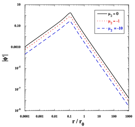
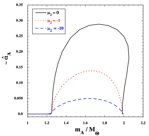
Figure 1: (Left) Field derivative $|\phi^{\prime}(r)|$ normalized by $M_{\rm Pl}/r_{0}$ in models of spontaneous scalarization with $\beta=-5$ for the SLy EOS with $\rho_{c}=8\rho_{0}$. Each line corresponds to $\mu_{2}=0,-1,-10$, respectively, where $\mu_{2}$ is normalized by $r_{0}^{2}/M_{\rm Pl}^{2}$. (Right) $-\hat{\alpha}_{A}$ versus $m_{A}/M_{\odot}$ for $\beta=-5$ and $\mu_{2}=0,-1,-10$. In this plot, the central matter density is in the range $\rho_{c}\leq 12\rho_{0}$. The negative coupling $\mu_{2}$ leads to the suppression of $-\hat{\alpha}_{A}$ in comparison to standard spontaneous scalarization ($\mu_{2}=0$).

In the left panel of Fig. 1, we plot the field derivative $|\phi^{\prime}(r)|$ (normalized by $M_{\rm Pl}/r_{0}$) with the central density $\rho_{c}=8\rho_{0}$ for $\beta=-5$ and $\mu_{2}=0$ (black line). In this case, the radius of NS is $r_{s}\simeq 0.13r_{0}=11.7$ km with the ADM mass $m_{A}\simeq 1.74M_{\odot}$, where $M_{\odot}$ is the solar mass. Deep inside the star ($r\ll r_{s}$), the scalar field varies according to Eq. (197), i.e., $\phi^{\prime}\simeq\beta\phi_{c}\rho_{c}(1-3w_{c})r/[6M_{\rm Pl}^{2}F(\phi_{c})]<0$ with $w_{c}=0.239$ and $\phi_{c}>0$. For $r\gg r_{s}$, the solution to $\phi$ is given by Eq. (210), i.e., $\phi^{\prime}(r)\simeq m_{A}\hat{\alpha}_{A}/[4\pi F(\phi_{0})M_{\rm Pl}r^{2}]<0$ with $\hat{\alpha}_{A}<0$. As we observe in Fig. 1, the two solutions smoothly join each other around $r=r_{s}$. The scalar field continuously decreases from the central value $\phi_{c}\simeq 0.2835M_{\rm Pl}$ to the asymptotic value $\phi_{0}$ close to 0 [which is in the range (226)]. In this case, the numerical value of $\hat{\alpha}_{A}$ is $-0.29$. The approximate analytic formula (225) gives the value $\hat{\alpha}_{A}\simeq-0.20$, so it is sufficient to estimate the order of the scalar charge.

The black line in the right panel of Fig. 1 shows $-\hat{\alpha}_{A}$ versus $m_{A}/M_{\odot}$ for $\beta=-5$ and $\mu_{2}=0$. With the central density in the range $\rho_{c}\lesssim 5.25\rho_{0}$, the scalar-field solution is close to the GR one ($\phi(r)=0$) and hence $|\hat{\alpha}_{A}|$ is much smaller than 1. For $\rho_{c}\gtrsim 5.25\rho_{0}$, which corresponds to the ADM mass $m_{A}\gtrsim 1.25M_{\odot}$, the scalarized branch starts to appear. With the increase of $\rho_{c}$, $-\hat{\alpha}_{A}$ grows to reach the maximum value $0.29$ around $\rho_{c}=8\rho_{0}$. As $\rho_{c}$ increases further, $-\hat{\alpha}_{A}$ starts to decrease and approaches 0 for $\rho_{c}\gtrsim 12\rho_{0}$. This is attributed to the fact that $w_{c}$ approaches $1/3$ in the analytic estimation of Eq. (225). For $\mu_{2}=0$, the observed orbital decay of binary pulsars put a stringent limit $\beta\geq-4.5$ Freire et al. (2012); Shao et al. (2017); Anderson et al. (2019). This bound arises from the scalar radiation of GWs induced by a large scalar charge. Note that the coupling constant $\beta=-5$, which corresponds to the black line shown in the right panel of Fig. 1, has been already excluded by binary pulsar measurements.

In the presence of the higher-order derivative term $\mu_{2}X^{2}$ with $\mu_{2}<0$, it is possible to reduce $|\hat{\alpha}_{A}|$. The scalar-field equation in the Einstein frame is given by Eq. (223), where the right hand-side is $\beta\phi(\hat{\rho}-3\hat{P})/(2M_{\rm Pl}^{2})$. When $\mu_{2}<0$, the stability condition (218) is always satisfied. Since the term $(1-3\mu_{2}\hat{h}\hat{\phi}^{\prime 2})\hat{h}$ gets larger for decreasing negative values of $\mu_{2}$, this leads to the suppression of $|\hat{\phi}^{\prime}|$ especially around the surface of star. Then, the scalar field decreases slowly around $r=r_{s}$. Hence we need to choose smaller values of $\phi_{c}$ to realize $\phi_{0}$ consistent with (226). In the left panel of Fig. 1, we plot $|\phi^{\prime}(r)|$ versus $r/r_{0}$ for $\beta=-5$ and $\mu_{2}=-1,-10$, where $\mu_{2}$ is normalized by $r_{0}^{2}/M_{\rm Pl}^{2}$. Since $\phi_{c}$ tends to be smaller for decreasing $\mu_{2}$, the term $\beta\phi_{c}(\hat{\rho}-3\hat{P})/(2M_{\rm Pl}^{2})$ is subject to suppression, which results in overall decrease of $|\phi^{\prime}(r)|$ both inside and outside the NS.

The suppression of $\phi_{c}$ induced by the negative coupling constant $\mu_{2}$ leads to the decrease of $|\hat{\alpha}_{A}|$ through Eq. (225). In the right panel of Fig. 1, we can confirm that, as $\mu_{2}$ decreases, $|\hat{\alpha}_{A}|$ gets smaller. For $\mu_{2}=-1$ and $\mu_{2}=-10$, the maximum numerical values of $|\hat{\alpha}_{A}|$ are 0.14 and 0.05, respectively. Thus, even when $\beta=-5$, it is possible to realize small values of $|\hat{\alpha}_{A}|$ that can be consistent with binary pulsar constraints. For the NS-BH binary with $m_{A}=1.7M_{\odot}$ and $m_{B}=2.5M_{\odot}$, the scalar charge with $|\hat{\alpha}_{A}|=0.05$ corresponds to the ppE parameter $\beta_{1}$ of order $|\beta_{1}|={\cal O}(10^{-6})$. If the future GW observations were to put limits on $\beta_{1}$ at this level, it is possible to probe the signature of spontaneous scalarization in the coupling ranges $\beta<-4.5$ and $\mu_{2}<0$.

VI.3.3 Massive theories with $m_{s}\neq 0$

Finally, we comment on theories with a nonvanishing scalar-field mass $m_{s}$. If $m_{s}$ is larger than the typical orbital frequency $\omega\simeq 10^{-13}$ eV during the inspiral phase of compact binaries, we showed in Sec. V.2 that the gravitational waveforms reduce to those in GR. For example, let us consider scalarized NSs realized by the coupling functions (183) with the potential (184) Minamitsuji and Tsujikawa (2022a). In this setup, the scalar field is in a state of symmetry restoration deep inside the NS due to the dominance of a positive nonminimal coupling ($\beta>0$) over a negative mass squared of the potential. Away from the star, the field settles down at its vacuum expectation value $\phi_{v}=\pi f_{B}$ with a positive mass squared $m_{s}^{2}$. In this scenario, the Compton radius $m_{s}^{-1}$ of the scalar field is of order the typical size of NS, i.e., $m_{s}^{-1}={\cal O}(10\,{\rm km})$, so that $m_{s}={\cal O}(10^{-11}~{}{\rm eV})$. Since $m_{s}$ is larger than the typical orbital frequency $\omega\simeq 10^{-13}$ eV, this model evades constraints from the observed gravitational waveform emitted during the inspiral phase.

There are also chameleon theories Khoury and Weltman (2004a, b) in which the effective mass of $\phi$ is large inside the star, while the field is light outside the star. If the mass $m_{s}$ outside the NS is smaller than the order $\omega\simeq 10^{-13}$ eV, there are next-to-leading order ppE parameters (170) arising from the correction term $m_{s}^{2}/\omega^{2}$ besides the leading-order ppE parameters (166). The gravitational waveforms in massive BD theories Alsing et al. (2012); Berti et al. (2012); Sagunski et al. (2018); Liu et al. (2020) and screened modified gravity in the Einstein frame Zhang et al. (2017); Liu et al. (2018); Niu et al. (2019) have been already studied in the literature. Our formulation in this paper can accommodate more general k-essence theories.

VII Conclusions

In this paper, we studied the gravitational waveform emitted during the inspiral phase of quasicircular compact binaries in a subclass of Horndeski theories. In this class of theories the speed of gravity $c_{t}$ is equivalent to that of light on the cosmological background, so it automatically evades observational bounds on $c_{t}$. Our general analysis accommodates not only (massive) BD theories and spontaneous scalarization but also k-essence and cubic derivative interactions. We exploited the PN expansion of a source energy-momentum tensor to derive solutions to the scalar-field perturbation from the source to the observer. In the presence of a cubic Galileon coupling $\mu_{3}X\square\phi$, our formulation is valid for the Vainshtein radius $r_{V}$ at most of order the star radius $r_{s}$.

In our theory there are no hairy BH solutions known in the literature, but nonminimal couplings $G_{4}(\phi)$ can give rise to NSs endowed with scalar charges. We have taken the description of point-like particles of the source whose mass $m_{I}$ depends on the scalar field, with $\alpha_{I}$ defined in Eq. (26). Due to the presence of nonminimal couplings in the Jordan frame, the combination $\hat{\alpha}_{I}=\alpha_{I}-g_{4}/2$ is a quantity directly related to the scalar charge, where $g_{4}$ is defined in Eq. (27). We clarified this point in Sec. VI by transforming the action (1) to that in the Einstein frame. The nonvanishing values of $\hat{\alpha}_{I}$ for NSs are crucial to probe the signature of modifications of gravity through the GW observations.

In Sec. III, we performed the expansion of metric and scalar field about a Minkowski background and derived the perturbation equations up to second order. We then obtained the quadrupole formula of tensor waves as Eq. (58), which reduces to the form (78) for a quasicircular orbit of the binary system. In Sec. IV, we showed that the solution to scalar-field perturbations up to quadrupole order is given by the sum of a massless mode (97) and a massive mode (98). The existence of scalar perturbations nonminimally coupled to gravity gives rise to breathing ($h_{b}$) and longitudinal ($h_{L}$) polarizations for the GW field, which are of the forms (122) and (123) respectively. We also derived solutions to the TT polarizations of GWs in the forms (119) and (120).

In Sec. V, we first discussed the energy loss induced by gravitational radiation and computed the time variation of an orbital frequency $\omega$. We then derived the gravitational waveform in Fourier space under a stationary phase approximation. If the scalar-field mass $m_{s}$ is much smaller than $\omega$, we obtained the waveforms of two TT polarizations as Eqs. (158) and (159) under the conditions (154) and (156). For $m_{s}\gg\omega$, the TT modes are practically equivalent to those in GR due to the absence of scalar radiation and the exponential suppression of fifth forces outside the star. In the massless limit $m_{s}/\omega\to 0$, we showed that the leading-order gravitational waveforms reduce to those in the ppE formalism, with the ppE parameters (166). If $m_{s}$ is not very much smaller than $\omega$, there are corrections to the ppE parameters given by Eq. (170).

In Sec. VI, we computed $\hat{\alpha}_{A}$ for NSs in several concrete theories to confront them with the future observations of GWs. In particular, we took into account a higher-order kinetic term $\mu_{2}X^{2}$ in $G_{2}$ for massless BD theories and theories of spontaneous scalarization. In BD theories, it is difficult to increase the scalar charge by the coupling $\mu_{2}$ due to the appearance of ghost or strong coupling problems. On the other hand, in theories of spontaneous scalarization, the negative coupling $\mu_{2}$ leads to the suppression of $|\hat{\alpha}_{A}|$ without inducing ghost instabilities (see the right panel of Fig. 1). For $\mu_{2}=0$, the binary pulsar measurements already put a tight bound $\beta\geq-4.5$ on the nonminimal coupling. The presence of $\mu_{2}X^{2}$ should make the theory compatible with binary pulsar observations even for $\beta<-4.5$. It remains to be seen how future events of the NS-BH binary system place bounds on the values of $\beta$ and $\mu_{2}$. Finally, we also showed that the recently proposed scalarized NSs realized in massive theories with $m_{s}={\cal O}(10^{-11}~{}{\rm eV})$ and $\beta>0$ give rise to gravitational waveforms similar to those in GR.

It will be of interest to apply our formula of gravitational waveforms to the cubic Galileon coupling with the Vainshtein radius $r_{V}\lesssim r_{s}$. Moreover, the extension of our analysis to full Horndeski theories allows us to accommodate more general modified gravity theories including the scalar-Gauss-Bonnet coupling Maselli et al. (2016); Pani et al. (2011); Kleihaus et al. (2014); Doneva and Yazadjiev (2018); Carson and Yagi (2020); Minamitsuji and Tsujikawa (2022b). We leave these topics for future works.