Neutrino Geoscience: Review, survey, future prospects

Abstract

The earth’s surface heat flux is 46 $\pm$ 3 TW (terrawatts, 10 ${}^{12}$ watts). Although many assume we know the earth’s abundance and distribution of radioactive heat producing elements (i.e., U, Th, and K), estimates for the mantle’s heat production varying by an order of magnitude and recent particle physics findings challenge our dominant paradigm. Geologists predict the earth’s budget of radiogenic power at 20 $\pm$ 10 TW, whereas particle physics experiments predict 15.3 ${}^{+4.9}_{-4.9}$ TW (KamLAND, Japan) and 38.2 ${}^{+13.6}_{-12.7}$ TW (Borexino, Italy).

We welcome this opportunity to highlight the fundamentally important resource offered by the physics community and call attention to the shortcomings associated with the characterization of the geology of the earth. We review the findings from continent-based, physics experiments, the predictions from geology, and assess the degree of misfit between the physics measurements and predicted models of the continental lithosphere and underlying mantle. Because our knowledge of the continents is somewhat uncertain (7.1 ${}^{+2.1}_{-1.6}$ TW), models for the radiogenic power in the mantle (3.5 to 32 TW) and the bulk silicate earth (crust plus mantle) continue to be uncertain by a factor of $\sim$ 10 and $\sim$ 4, respectively. Detection of a geoneutrino signal in the ocean, far from the influence of continents, offers the potential to resolve this tension. Neutrino geoscience is a powerful new tool to interrogate the composition of the continental crust and mantle and its structures.

\draftfalse\journalname

Reviews of Geophysics

Research Center for Neutrino Science, Tohoku University, Sendai, Miyagi, 980-8578, Japan Department of Earth Sciences, Tohoku University, Sendai, Miyagi, 980-8578, Japan Department of Geology, University of Maryland, College Park, MD 20742, USA

\correspondingauthor

William McDonoughmcdonoug@umd.edu

{keypoints}

Parameters influencing the geological interpretation of a geoneutrino signal

Problems with establishing the mantle contribution to the geoneutrino signal

Importance of taking a geoneutrino flux measurement in the ocean far from the continents

Author ORCID numbers are

William F. McDonough :	0000-0001-9154-3673
Hiroko Watanabe :	0000-0002-2363-5637

AGU Book chapter:
Core-Mantle Coevolution: A Multidisciplinary approach
Editors: Takashi Nakagawa and Madhusoodhan Satish Kumar

Plain language summary

Potassium, thorium, and uranium are radioactive and heat is given off during their decay. This release of energy drives the earth’s dynamic processes of plate tectonics, mantle convection, and the geodynamo, with the latter generating the protective magnetic shield surrounding the planet. The earth is a hybrid vehicle powered by primordial and radiogenic energy, with the former from impacts during planet building and the latter from radioactive decays. Unfortunately, we lack a fuel gauge for either energy source and consequently we do not know how much power is left to drive the earth’s engine, nor how much energy (and time) is left to keep it habitable?

Geoneutrinos are naturally occurring electron antineutrinos produced during $\beta^{-}$ (and $EC$ , electron capture) decays of these heat producing elements. These tiny fundamental particles are almost impossible to detect, because they are about a billion times smaller than a proton, near-massless and chargeless. In 2005, particle physicists first detected the earth’s emission of geoneutrinos with a large underground detector and are now telling us about the amount of radiogenic heat inside the earth [araki2005experimental]. Reading the earth’s fuel gauge by counting geoneutrinos, however, requires that geologists understand the abundance and distribution of these heat producing elements in the continents and mantle.

New results from geoneutrino detectors in Japan and Italy present contrasting stories as to how much fuel is left in the earth’s engine. Geologists are building 3-D physical and chemical models of the earth, but are vexed by the subsurface complexities of the continents. Efforts are underway to construct an ocean-going geoneutrino detector that can independently measure the mantle’s flux, far from the influence of continents, and define how much radiogenic fuel is left in the earth.

1 Introduction

Core-mantle evolution involves understanding earth’s differentiation processes, which established the present day distribution of the heat producing elements, and its dynamic consequences (i.e., the radiogenic heat left in the mantle powering mantle convection, plate tectonics, and the geodynamo). The energy to drive the earth’s engine comes from two different sources: primordial and radiogenic. Primordial energy represents the kinetic energy inherited during accretion and core formation. Radiogenic energy is the heat of reaction from nuclear decay. We do not have a constraint on the proportion of these different energy sources driving the present day earth’s dynamics. In turn, this means that we do not have sufficient constraint on the thermal evolution of the planet, aside from first order generalities. You might ask, is this important? We ask the question – how much energy (and time) is left to keep the earth habitable?

We understand that the earth started out hot due to abundant accretion energy, the gravitational energy of sinking metal into the center, a giant impact event for the formation of the earth’s Moon, and energy from short-lived (e.g., ${}^{26}$ Al and ${}^{60}$ Fe) and long-lived (K, Th, and U) radionuclides. From this hot start the planet should quickly lose some of its initial energy, although the amount and rate are unknowns. There are many significant unknowns regarding the thermal evolution of the earth: (1) the nature and presence (or absence) and lifetime of an early atmosphere, which has a thermal blanketing effect; (2) the compositional model for the earth, particularly the absolute abundances of the heat-producing elements (HPE: K, Th, & U); (3) the cooling rate of the mantle (present day estimates: 100 $\pm$ 50 K/Ga); and (4) the rate of crust formation and thus extraction of HPEs from the mantle.

The recent recognition [KRAUSS] and subsequent detection [araki2005experimental] of the planet’s geoneutrino emission has opened up a new window into global scale geochemistry of the present day earth. The measurement of this flux presents earth scientists with a transformative opportunity for new insights into the composition of the earth and its energy budget. For the most part, solid earth geophysics measures and parameterizes the present day state of the planet. In contrast, solid earth geochemistry measures and parameterizes its time integrated state, mostly on a hand sample scale and then extrapolates these insights to larger scales. The advent of measuring the earth’s geoneutrino flux allows us, for the first time, to get a global measure of its present day amount of Th and U.

This paper is organized as follows: we provide the rationale for the field of neutrino geoscience and define some terms (Section 2). We review the existing and developing detectors, the present-day detection methods and future technologies (Section 3). We discuss the latest results from the physics experiments (Section 4). We present the range of compositional models proposed for the earth (Section 5) followed by a discussion of the geological prediction of the geoneutrino fluxes at various detectors (Section 6). We finish with a discussion on determining the radioactive power in the mantle (Section 7) and future prospects (Section 8).

2 Neutrino Geoscience

The field of neutrino geoscience focuses on constraining the earth’s abundances of Th and U and with these data we can determine: (1) the absolute concentration of refractory elements in the earth and from that determine the bulk silicate earth’s composition (BSE; crust plus mantle), and (2) the amount of radiogenic power in the earth driving the planet’s major dynamic processes (e.g., mantle convection, plate tectonics, magmatism, and the geodynamo). These two constraints set limits on the permissible models for the composition of the earth and its thermal evolutionary history.

First, the refractory elements are in constant relative abundances in all chondrites. There are 36 of these elements (e.g., Al, Ca, Sr, Zr, REE, Th & U) and by establishing the absolute abundance of one defines all abundances, since refractory elements exist in constant ratios to each other [McDonough1995]. Most of these elements are concentrated in the bulk silicate earth, but not all (e.g., Mo, W, Ir, Os, Re, etc) and these latter ones are mostly concentrated in the metallic core. Knowing the earth’s abundance of Ca and Al, two of the eight most abundant elements (i.e., O, Fe, Mg, Si, Ca, Al, Ni, and S) that make up terrestrial planets (i.e., 99%, mass and atomic proportions), defines and restricts the range of accepted compositional models of the bulk earth and BSE.

Second, the the decay of ${}^{40}$ K, ${}^{232}$ Th, ${}^{238}$ U, and ${}^{235}$ U (i.e., HPE) provides the earth’s radiogenic power, accounts for 99.5% of its total radiogenic power, and is estimated to be ( $19.9\pm 3.0$ ) TW (1 TW = 10 ${}^{12}$ watts). This estimate, however, assumes a specific BSE model composition [McDonough1995, palme2014cosmochemical]. It must be noted that there is no consensus on the composition of the BSE, and so predictions from competing compositional models span from about 10 to 38 TW [javoy2010chemical, agostini:2020]. This uncertainty in our present state of knowledge means that the field of neutrino geoscience plays a crucial role in resolving fundamental questions in earth sciences.

2.1 Background Terms

The field of neutrino geoscience spans the disciplines of particle physics and geoscience, including geochemistry and geophysics. The following list of terms are offered to support this interdisciplinary research field.

alpha ( $\alpha$ ) decay: a radioactive decay process that reduces the original nuclide ( $X$ ) by 4 atomic mass units by the emission of a ${}^{4}_{2}$ He nucleus and reaction energy ( $Q$ ). Commonly, the $\alpha$ particle is emitted with between 4 and 9 MeV (1 MeV = 10 ${}^{6}$ eV) of discrete kinetic energy. The basic form of $\alpha$ decay is:

\begin{split}\textrm{Alpha}\quad(\alpha)\qquad&{}^{A}_{Z}X\rightarrow\;^{A-4}_{Z-2}X^{\prime}+\alpha+Q\\ \end{split}

(1)

beta decay : a radioactive decay process that transforms the original nuclide ( $X$ ) into an isobar (same mass $A$ ) with the next lower proton number ( $Z$ ) during either electron capture ( $EC$ ) or $\beta^{+}$ decays or alternatively, the next higher proton number ( $Z$ ) during $\beta^{-}$ decay. During each decay, there is an exchange of two energetic leptons (i.e., beta particles) and reaction energy ( $Q$ ). Basic forms are:

\begin{split}\textrm{Beta Minus}\quad(\beta^{-})\qquad&{}^{A}_{Z}X\rightarrow^{A}_{Z+1}X^{\prime}+e^{-}+\mathit{{\mkern 4.0mu\overline{\mkern-4.0mu{\nu}}}{}_{\mspace{-2.0mu}\scriptstyle{\!e}}^{\mspace{0.0mu}\scriptstyle{}}}+Q,\\ \textrm{Electron Capture}\quad(\textrm{$EC$})\qquad&{}^{A}_{Z}X+e^{-}\rightarrow^{A}_{Z-1}X^{\prime}+\mathit{{\nu}{}_{\mspace{-3.0mu}\scriptstyle{\!e}}^{\mspace{-1.0mu}\scriptstyle{}}}+Q,\\ \textrm{Beta Plus}\quad(\beta^{+})\qquad&{}^{A}_{Z}X\rightarrow^{A}_{Z-1}X^{\prime}+e^{+}+\mathit{{\nu}{}_{\mspace{-3.0mu}\scriptstyle{\!e}}^{\mspace{-1.0mu}\scriptstyle{}}}+Q\\ \end{split}

(2)

beta particles : First generation energetic leptons, either matter leptons (electrons and neutrinos: $e^{-}$ and $\mathit{{\nu}{}_{\mspace{-3.0mu}\scriptstyle{\!e}}^{\mspace{-1.0mu}\scriptstyle{}}}$ ) or antimatter leptons (positrons and antineutrinos: $e^{+}$ and $\mathit{{\mkern 4.0mu\overline{\mkern-4.0mu{\nu}}}{}_{\mspace{-2.0mu}\scriptstyle{\!e}}^{\mspace{0.0mu}\scriptstyle{}}}$ ).

chondrite: an undifferentiated stony meteorite containing chondrules (flash-melted spheres, sub-mm to several mm across), matrix (fine grained (micron scale) aggregate of dust and crystals), and sometimes Ca-Al-inclusions and other refractory phases. They are typically mixtures of silicates and varying amounts of Fe-Ni alloys and classified into groups based on their mineralogy, texture, and redox state. Three dominant groups are the carbonaceous, ordinary, and enstatite type chondrites, from most oxidized to reduced, respectively. Isotopic observations are also used to create a twofold classification of chondrites and related meteorites (i.e., the NC and CC groups). The NC (non-carbonaceous) group include enstatite and ordinary chondrites and are believed to have formed in the inner solar system inside of Jupiter. The CC (carbonaceous) group include carbonaceous chondrites and are believed to have formed in the outer solar system from Jupiter and beyond. The CI carbonaceous chondrite type (the sole chondrite type lacking chondrules) is considered most primitive because its element abundances matches that of the solar photosphere 1:1 over 6 orders of magnitude, except for the noble and H-C-N-O gases.

geoneutrinos: naturally occurring electron antineutrinos ( $\mathit{{\mkern 4.0mu\overline{\mkern-4.0mu{\nu}}}{}_{\mspace{-2.0mu}\scriptstyle{\!e}}^{\mspace{0.0mu}\scriptstyle{}}}$ , with the over-bar indicating it is an antimatter particle), mostly, and electron neutrinos ( $\mathit{{\nu}{}_{\mspace{-3.0mu}\scriptstyle{\!e}}^{\mspace{-1.0mu}\scriptstyle{}}}$ ), much less so, produced during $\beta^{-}$ , and [ $EC$ and $\beta^{+}$ ] decays, respectively. The interaction cross-sections, which scale with their energy, for the detectable geoneutrinos (i.e., Th and U) are on the order of 10 ${}^{-47}$ m ${}^{2}$ . Consequently, these particles rarely interact with matter in the earth. The earth’s geoneutrino flux is 10 ${}^{25}$ $\mathit{{\mkern 4.0mu\overline{\mkern-4.0mu{\nu}}}{}_{\mspace{-2.0mu}\scriptstyle{\!e}}^{\mspace{0.0mu}\scriptstyle{}}}$ s ${}^{-1}$ [mcdonough2020radiogenic]. Each neutrino leaving the earth removes a portion of the earth’s radiogenic heat ( $Q$ ).

heat producing elements (HPE): potassium, thorium, and uranium (i.e., K, Th, and U, or more specifically ${}^{40}$ K, ${}^{232}$ Th, ${}^{235}$ U, and ${}^{238}$ U) account for $\sim$ 99.5% of the earth’s radiogenic heating power.

Inverse Beta Decay (IBD): a nuclear reaction used to detect electron antineutrinos in large underground liquid scintillation detectors that are surrounded by thousands of photomultiplier tubes. The reaction [ $\mathit{{\mkern 4.0mu\overline{\mkern-4.0mu{\nu}}}{}_{\mspace{-2.0mu}\scriptstyle{\!e}}^{\mspace{0.0mu}\scriptstyle{}}}+p\rightarrow e^{+}+n$ ] involves a free proton (i.e., H atom) capturing a through going $\mathit{{\mkern 4.0mu\overline{\mkern-4.0mu{\nu}}}{}_{\mspace{-2.0mu}\scriptstyle{\!e}}^{\mspace{0.0mu}\scriptstyle{}}}$ and results in two flashes of light close in space and time. The first flash of light involves $e^{+}-e^{-}$ annihilation (order a picosecond following $\mathit{{\mkern 4.0mu\overline{\mkern-4.0mu{\nu}}}{}_{\mspace{-2.0mu}\scriptstyle{\!e}}^{\mspace{0.0mu}\scriptstyle{}}}+p$ interaction) and the second flash ( $\sim$ 0.2 ms later) comes from the capture by a free proton of the thermalizing neutron. This coincidence of a double light flash in space and time, with the second flash having 2.2 MeV light, reduces the background by a million-fold. This reaction requires the $\mathit{{\mkern 4.0mu\overline{\mkern-4.0mu{\nu}}}{}_{\mspace{-2.0mu}\scriptstyle{\!e}}^{\mspace{0.0mu}\scriptstyle{}}}$ to carry sufficient energy to overcome the reaction threshold energy of $E_{\bar{\nu}_{e}}^{thr}=1.8$ MeV. Thus, restricting us to detecting only antineutrinos from the $\beta^{-}$ decays in the ${}^{238}$ U and ${}^{232}$ Th decay chains.

major component elements: a cosmochemical classification term for Fe, Ni, Mg, & Si, with half-mass condensation temperatures ( $T_{\mathrm{c}})$ between 1355 and 1250 K. These elements condense from a cooling nebular gas into silicates (first olivine, then pyroxene) and Fe, Ni alloys and together with oxygen represents $\geq$ 93% of terrestrial planet’s mass [mcdonough2021tp].

Earth and its parts: the earth is chemically differentiated. It has a metallic core surrounded by the bulk silicate earth (BSE, aka, Primitive Mantle), which initially included the mantle, oceanic and continental crust, and the hydrosphere & atmosphere; the Primitive Mantle is the undegassed and undifferentiated earth minus the core. The present day silicate earth, less the hydrosphere and atmosphere, is made up of the mantle, including its conductive layers at the bottom (D”), and the top lithosphere; the latter composed of the crust an underlying lithospheric mantle. The lithosphere is the mechanically stiff (i.e., $>$ 10 ${}^{5}$ higher viscosity than the underlying asthenospheric mantle), thermally conductive boundary layer. In the continents, the zone above the Moho (a seismically defined boundary between the crust and mantle) is the continental crust and below the continental lithospheric mantle (CLM). Masses and thicknesses of these domains are listed in Table 1.

Table 1: Mass of the Earth and its parts

Domain/reservoir	thickness	mass	citation ${}^{\dagger}$
	km ( $\pm$ )	kg ( $\pm$ )
Earth	6371 ( ${}^{+7}_{-20}$ )	5.97218 (60) $\times$ 10 ${}^{24}$	[1]
bulk silicate earth (BSE)	2895 (5)	4.036 (6) $\times$ 10 ${}^{24}$	[2]
Modern mantle (DM + EM domains) ${}^{*}$	2867 (20) ${}^{\ddagger}$	4.002 (20) $\times$ 10 ${}^{24}$	[2]
oceanic crust ${}^{\#}$	10.5 (4.3)	0.92 (0.11) $\times$ 10 ${}^{22}$	[3]
continental crust ${}^{\#}$	40 (9)	2.22 (26) $\times$ 10 ${}^{22}$	[3]
continental lithospheric mantle (CLM)	115 (80)	6.3 (0.8) $\times$ 10 ${}^{22}$	[3]

${}^{\dagger}$ cited source: 1 = \citeAchambat2010, 2= \citeAdziewonski1981preliminary, 3 = \citeAWipperfurth2020
${}^{*}$ DM = Depleted Mantle, the chemically depleted source of MORB (mid-ocean ridge basalts), which is viewed as the chemical complement to the continental crust, and
${}^{*}$ EM = Enriched Mantle, a smaller (i.e., $\frac{1}{5}$ mass), deeper, and more chemically enriched source of OIB (ocean island basalts).
${}^{\ddagger}$ from PREM, assuming a uniform surface crust of 24 km
${}^{\#}$ Using a LITHO1.0 model, see Table 1 in \citeAWipperfurth2020.

moderately volatile elements: a cosmochemical classification term for elements with half-mass condensation temperatures ( $T_{\mathrm{c}})$ between 1250 and 600 K. These elements include the alkali metals (lithophile), some transition metals, all the other metals, less Al, and the pnictogens and chalcogens, less N and O.

primordial energy: the energy in the earth from accretion and core formation. Accretion kinetic energy is $\sim$ 10 ${}^{32}$ J, assuming an earth mass (5.97 $\times$ 10 ${}^{24}$ kg) and 10 km/s as an average velocity of accreting particles. The gravitational energy of core formation, which translates to heating energy, is $\approx$ 10 ${}^{30}$ J, depending on the assumed settling velocity of a core-forming metal in the growing earth.

radiogenic energy: energy of a nuclear reaction ( $Q$ ) resulting from radioactive decay, given in units of MeV (1 MeV = 10 ${}^{6}$ eV) or pJ (1 pJ = 10 ${}^{-12}$ J), where 1MeV = 0.1602 pJ. For $\beta$ decays $Q$ (MeV) = (mass ${}_{p}$ - mass ${}_{d}$ ) $\times$ 931.494, with mass ${}_{p}$ (mass of parent isotope), mass ${}_{d}$ (mass of daughter isotope) in atomic mass units (1 amu = 1.660539 $\times$ 10 ${}^{-27}$ kg = 931.494 MeV) and for $\alpha$ decay, $Q$ (MeV) = (mass ${}_{p}$ - mass ${}_{d}$ - mass ${}_{\alpha}$ ) $\times$ 931.494, where $E=eV/c^{2}$ , or 1 amu = 0.931494 GeV/c ${}^{2}$ .

refractory elements: a cosmochemical classification term for elements with half-mass condensation temperatures ( $T_{\mathrm{c}})>$ 1355 K; they condense at the earliest stage of the cooling of high-temperature nebular gas. These elements are in equal relative proportion ( $\pm$ 15%) in chondritic meteorites. In terrestrial planets, many of these elements are classified as lithophile (dominantly coupling with oxygen and hosted in the crust and mantle), or siderophile (dominantly metallically bonded and hosted in the core). The refractory elements include: Be, Al, Ca, Ti, Sc, V, Sr, Y, Zr, Nb, Mo, Rh, Ru, Ba, REE, Hf, Ta, W, Re, Os, Ir, Pt, Th and U. The core contains $\geq$ 90% of the earth’s budget of Mo, Rh, Ru, W, Re, Os, Ir, and Pt, about half of its V, and potentially a minor fraction of its Nb.

surface heat flux: the total surface heat flux from the earth’s interior is reported as 46 $\pm$ 3 TW [jaupart:2015tg] or 47 $\pm$ 2 TW [davies2013global]. On average the surface heat flux is about 86 mW/m ${}^{2}$ , with that for the continents being 65 mW/m ${}^{2}$ and for the oceans being 96 mW/m ${}^{2}$ [davies2013global]. Energy contributions to this surface flux come from the core (primordial, plus a minor ( $\sim$ 1% of the surface total) amount due to inner core crystallization), mantle (a combination of primordial and radiogenic), and crust (radiogenic). Other contributions include negligible additions from tidal heating and crust - mantle differentiation.

3 Detectors and detection technology

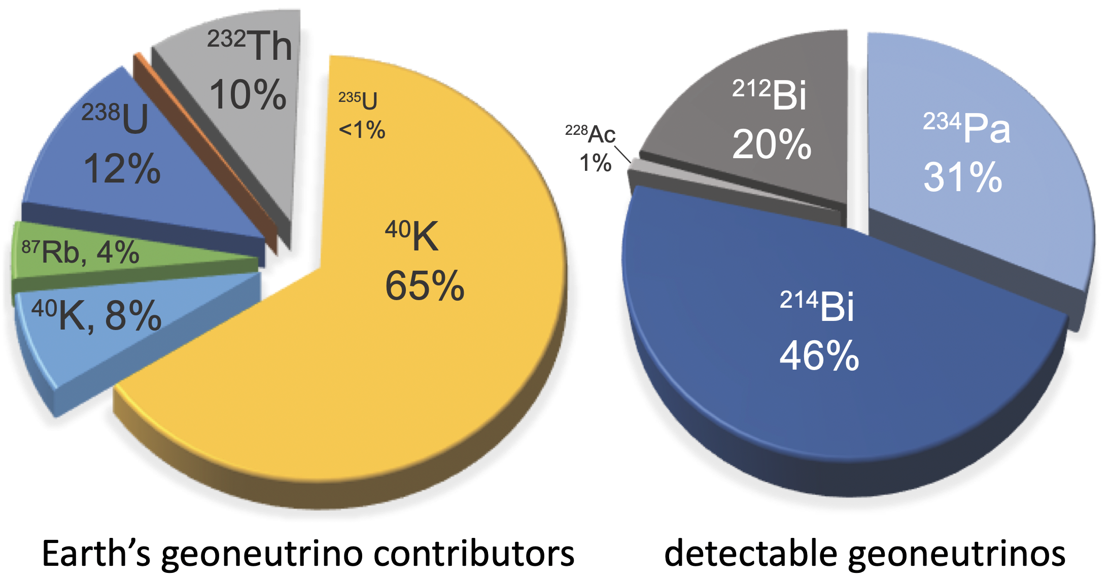
Electron antineutrinos ( $\mathit{{\mkern 4.0mu\overline{\mkern-4.0mu{\nu}}}{}_{\mspace{-2.0mu}\scriptstyle{\!e}}^{\mspace{0.0mu}\scriptstyle{}}}$ ) come mostly from the radioactive decays of ${}^{40}$ K, ${}^{232}$ Th, ${}^{235}$ U, and ${}^{238}$ U [<]i.e., geoneutrinos; ¿KRAUSS, plus contributions from local anthropogenic sources (i.e., nuclear reactor plants). The earth emits some 10 ${}^{25}$ s ${}^{-1}$ geoneutrinos [mcdonough2020radiogenic], with 65% coming from $\beta^{-}$ decays of ${}^{40}$ K (Figure 1).

Refer to caption — Figure 1: Relative proportions of the earth’s present‐day flux of naturally occurring geoneutrinos (left) and the detectable geoneutrinos (right) from the ${}^{232}$ Th decay chain (grey; ${}^{228}$ Ac and ${}^{212}$ Bi) and ${}^{238}$ U decay chain (blue; ${}^{234}$ Pa and ${}^{214}$ Bi, not shown is the negligible contribution from ${}^{212}$ Tl) (see also Table 2). ${}^{40}$ K has two branches: $\beta^{-}$ to ${}^{40}$ Ca (65%) and $EC$ to ${}^{40}$ Ar (8%).

The detection of an electron antineutrino uses the Inverse Beta Decay (IBD) reaction: $\mathit{{\mkern 4.0mu\overline{\mkern-4.0mu{\nu}}}{}_{\mspace{-2.0mu}\scriptstyle{\!e}}^{\mspace{0.0mu}\scriptstyle{}}}+p\rightarrow e^{+}+n$ , which has a reaction threshold energy of $E_{\bar{\nu}_{e}}^{thr}=1.806$ MeV.

E_{\bar{\nu}_{e}}^{thr}=\frac{(M_{n}+m_{e})^{2}-M^{2}_{p}}{2M_{p}}=1.806[MeV]

(3)

assuming the laboratory frame (i.e., stationary target) and where $M_{p}$ , $M_{n}$ , and $m_{e}$ are the masses of the proton (938.272 MeV), neutron (939.565 MeV) and electron (0.5110 MeV). The neutrino mass is unknown and contributes negligibly to this reaction. Although its upper limit is 0.8 $eV/c^{2}$ [aker2021direct], estimates of the neutrino’s mass is of the order of 10s to 100s of $meV$ [Nu_mass-ordering18]. This energy threshold restricts the detectable antineutrinos to $\beta^{-}$ decays from the ${}^{238}$ U and ${}^{232}$ Th decay chains (Figure 1).

3.1 Technical details for detecting geoneutrinos

Here we highlight some relevant aspects of the detection scheme.

Detection occurs when an antineutrino interacts with a free proton, transforming it to a neutron plus a positron, which then causes two flashes of light close in space and time. Each flash of light occurring in these large liquid scintillation spectrometers, which are sited 1 to 2 km underground to shield them from descending, atmospherically produced muons, are detected by the thousands of photomultiplier tubes covering the inner walls, each facing the detector’s central volume.

Energy conservation requires that $E_{\mathit{{\mkern 4.0mu\overline{\mkern-4.0mu{\nu}}}{}_{\mspace{-2.0mu}\scriptstyle{\!e}}^{\mspace{0.0mu}\scriptstyle{}}}}$ + $M_{p}$ = $T_{e^{+}}$ + $m_{e}$ + $M_{n}$ + $T_{n}$ , with $T_{e^{+}}$ and $T_{n}$ being the kinetic energy of the positron and neutron. The prompt event involves the positron being annihilated in picoseconds by an electron, with the signal being the sum of the reaction releasing a 1.022 MeV energy flash (the sum of the masses of these two leptons) plus the characteristic kinetic energy inherited by the positron from the antineutrino ( $E_{prompt}$ = ( $E_{\mathit{{\mkern 4.0mu\overline{\mkern-4.0mu{\nu}}}{}_{\mspace{-2.0mu}\scriptstyle{\!e}}^{\mspace{0.0mu}\scriptstyle{}}}}$ + $M_{p}$ - $m_{e}$ - $M_{n}$ - $T_{n}$ ) + 2 $m_{e}$ , or = $E_{\mathit{{\mkern 4.0mu\overline{\mkern-4.0mu{\nu}}}{}_{\mspace{-2.0mu}\scriptstyle{\!e}}^{\mspace{0.0mu}\scriptstyle{}}}}$ - $T_{n}$ - 0.782[MeV]). The accompanying emitted neutron undergoes a cascade of collisions (thermalizing events, loss of energy to its surroundings as it goes towards thermal equilibrium) over about 200 $\mu$ s and approximately 15 cm from the initial interaction point. This neutron is ultimately captured by a second free proton creating ${}^{2}$ H, resulting in a 2.22 MeV (binding energy) flash. This rare event sequence is eminently detectable because of its characteristics: two flashes of light in space and time, with the second flash having a specific energy. This reaction chain eliminates most background and improves the signal to noise ratio by a million fold.

The organic liquid scintillator is mostly a long chain, aromatic ring hydrocarbon with approximately an H:C proportion of $\sim$ 2. A wavelength shifting fluor compound is added to the scintillator to set the fluorescence peak emission at $\sim$ 350-400 nm in order to reach the maximum quantum efficiency of the photomultiplier tubes. The photon yield for the liquid scintillator is typically a light yield of 200 to 400 photons/MeV.

The interaction cross section of antineutrinos (and neutrinos) scales with their energy. For each $\beta^{-}$ decay there is a spectrum of $\mathit{{\mkern 4.0mu\overline{\mkern-4.0mu{\nu}}}{}_{\mspace{-2.0mu}\scriptstyle{\!e}}^{\mspace{0.0mu}\scriptstyle{}}}$ emitted energies, which in turn means a spectrum of interaction cross-sections. For IBD detection (i.e., starting at 1.806 MeV), the probability of a geoneutrino detection is low (order 1/10 ${}^{19}$ ), given that their cross sections are between 10 ${}^{-48}$ and 10 ${}^{-46}$ m ${}^{2}$ [vogel1999angular]. The overall emission above the energy threshold level are 0.40 U $\mathit{{\mkern 4.0mu\overline{\mkern-4.0mu{\nu}}}{}_{\mspace{-2.0mu}\scriptstyle{\!e}}^{\mspace{0.0mu}\scriptstyle{}}}$ per decay and 0.156 Th $\mathit{{\mkern 4.0mu\overline{\mkern-4.0mu{\nu}}}{}_{\mspace{-2.0mu}\scriptstyle{\!e}}^{\mspace{0.0mu}\scriptstyle{}}}$ per decay. There are four decay chains which produce detectable antineutrinos: two from the ${}^{232}$ Th and two from the ${}^{238}$ U decay chains (Table 2). The BSE has a Th/U mass ratio of 3.77 (or molar Th/U = 3.90) [wipperfurth:2018]. However, despite Th being four times more abundant than U, attributes of the IBD detection method (i.e., $E_{\mathit{{\mkern 4.0mu\overline{\mkern-4.0mu{\nu}}}{}_{\mspace{-2.0mu}\scriptstyle{\!e}}^{\mspace{0.0mu}\scriptstyle{}}}}$ , branching fraction, and $\sigma_{IBD}$ ) makes U much easier to detect.

Table 2: Detectable

\mathit{{\mkern 4.0mu\overline{\mkern-4.0mu{\nu}}}{}_{\mspace{-2.0mu}\scriptstyle{\!e}}^{\mspace{0.0mu}\scriptstyle{}}}

events

$\beta^{-}$ decay	$\mathit{{\mkern 4.0mu\overline{\mkern-4.0mu{\nu}}}{}_{\mspace{-2.0mu}\scriptstyle{\!e}}^{\mspace{0.0mu}\scriptstyle{}}}$ Max E ${}^{\dagger}$	branching	Max IBD cross section ${}^{\ddagger}$	% of total ${}^{*}$
events	(MeV)	fraction	$\sigma_{IBD}$ (10 ${}^{-43}$ cm ${}^{2}$ )	$\mathit{{\mkern 4.0mu\overline{\mkern-4.0mu{\nu}}}{}_{\mspace{-2.0mu}\scriptstyle{\!e}}^{\mspace{0.0mu}\scriptstyle{}}}$ signal
		${}^{232}$ Th decay chain
${}^{228}$ Ac $\rightarrow$ ${}^{228}$ Th	2.134	1.00	4.3	1
${}^{212}$ Bi $\rightarrow$ ${}^{212}$ Po	2.252	0.64	4.8	20
		${}^{238}$ U decay chain
${}^{234}$ Pa $\rightarrow$ ${}^{234}$ U	2.197	1.00	4.6	31
${}^{214}$ Bi $\rightarrow$ ${}^{214}$ Po	3.270	1.00	33	46
${}^{212}$ Tl $\rightarrow$ ${}^{212}$ Po	4.391	0.0002	90	$<<$ 1%

${}^{\dagger}$ there is a spectrum of energies for each antineutrino generated during a $\beta^{-}$ decay, where typically the $\mathit{{\mkern 4.0mu\overline{\mkern-4.0mu{\nu}}}{}_{\mspace{-2.0mu}\scriptstyle{\!e}}^{\mspace{0.0mu}\scriptstyle{}}}$ takes about $\frac{2}{3}$ and the $e^{-}$ about $\frac{1}{3}$ of the reaction energy ( $Q$ ).
${}^{\ddagger}$ as the energy of the antineutrino decreases so does its interaction cross-section.
${}^{*}$ numbers from Tables 3 and 5 in \citeAfiorentini2007geo.

3.2 Detectors: Existing, being built, being planned

Currently there are two detectors (Fig. 2) measuring the earth’s geoneutrino flux: KamLAND (1 kton), in Kamioka, Japan [araki2005experimental, KAMLAND19], and SNO+ (1 kton) in Sudbury, Ontario, Canada [SNO+] experiments. The Borexino detector (0.3 kton), in Gran Sasso, Italy [agostini:2020], has finished. The JUNO (20 kton) experiment in Jiangmen, Guangdong province, China [an2016] is currently being built. The Jinping ( $\sim$ 4 kton) experiment in Jinping Mountains, Sichuan province, China [Beacom_2017] is in development, with prototype detectors onsite testing future detector materials and technologies. Detectors in the proposal stage include Baksan in the Caucasus mountains in Russia [domogatsky2005neutrino], Andes in Agua Negra tunnels linking the borders of Chile and Argentina [ANDES], and a proposed ocean bottom detector. Significantly, the Andes detector is the only proposed detector to be sited in the southern hemisphere.

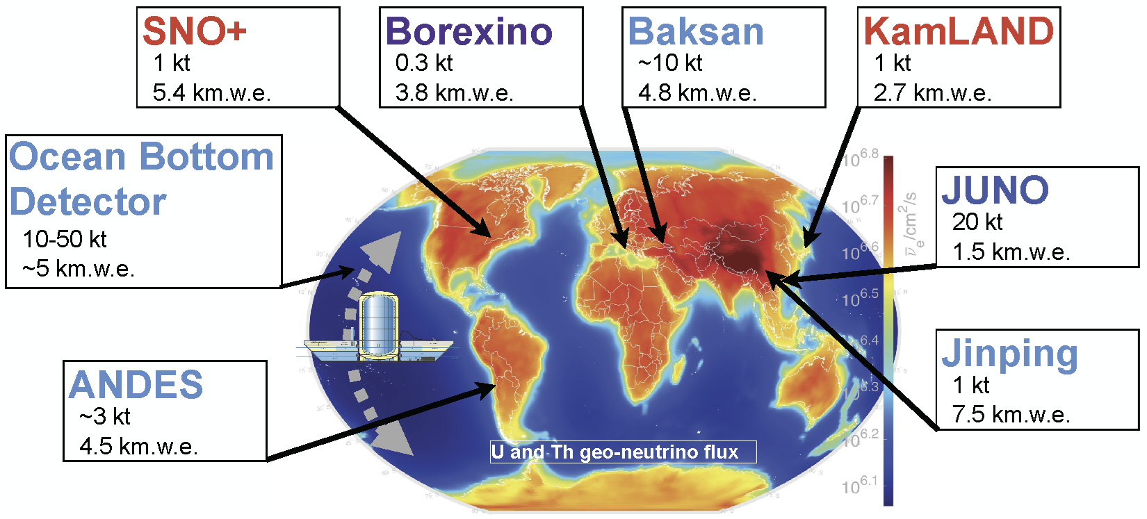
There are ongoing developments for a ocean-going detector. A team of particle physicists from the University of Hawaii put forth a proposal more than 10 years ago for an ocean bottom detector called Hanohano [Learned]. A team of Japanese particle physicists and engineers and earth scientists from JAMSTEC (Japan Agency for Marine-Earth Science and Technology) are currently moving forward with a project to deploy and test a mobile prototype detectors (“Ocean Bottom Detector” (OBD) scale is not yet set, but envisaged to up to 1 ton) off the coast of Japan. A mobile ocean-going detector offers a complementary measurement to land-based experiments. By sitting in the middle of the Pacific Ocean, 3000 km from South America, 3000 km from Australia, and $\sim$ 3000 km from the core-mantle boundary, such a detector gets a “mostly-mantle” signal.

4 Latest results from the physics experiments

Results from the physics experiments follow counting statistics, with increasing exposure (time spent counting) uncertainties reduce. These experiments are attentive to systematic and statistical uncertainties and addressed these issues in great detail in their publications.

The measured geoneutrino flux is reported in $\mathit{{\mkern 4.0mu\overline{\mkern-4.0mu{\nu}}}{}_{\mspace{-2.0mu}\scriptstyle{\!e}}^{\mspace{0.0mu}\scriptstyle{}}}$ cm ${}^{-2}$ $\mu s^{-1}$ for the KamLAND experiment and in TNU (Terrestrial Neutrino Unit) for the Borexino experiments. \citeAMantovani2004 introduced TNU as a way to normalize the differences between detectors. A 1 TNU signal represents the detection of one event in a 1 kiloton liquid scintillation detector over a one year exposure with a 100% detection efficiency. A 1 kiloton liquid scintillation detector has $\sim$ 10 ${}^{32}$ free protons (the detection target). Each detector has its own efficiency relative to a 1 kiloton fiducial volume detector, which accounts for the differences in the size of detector, its photomultiplier coverage, its response efficiency of the scintillator, and other factors. The conversion factor between signal in TNU and flux in $\mathit{{\mkern 4.0mu\overline{\mkern-4.0mu{\nu}}}{}_{\mspace{-2.0mu}\scriptstyle{\!e}}^{\mspace{0.0mu}\scriptstyle{}}}$ cm ${}^{-2}$ $\mu s^{-1}$ depends on the Th/U ratio and has a value of 0.11 $\mathit{{\mkern 4.0mu\overline{\mkern-4.0mu{\nu}}}{}_{\mspace{-2.0mu}\scriptstyle{\!e}}^{\mspace{0.0mu}\scriptstyle{}}}$ cm ${}^{-2}$ $\mu s^{-1}$ TNU ${}^{-1}$ for earth’s Th/U ${}_{molar}$ of 3.9.

The most recent results for the KamLAND and Borexino experiments are 32.1 $\pm$ 5.0 [KAMLAND19] and 47.0 ${}^{+8.4}_{-7.7}$ [agostini:2020] TNU, respectively. [The SNO+ detector began counting in 2020 with a partial filled volume (with delays due to the covid-19 pandemic) and is yet to report their data.] The conversion between TNU and TW depends on the geological model assumed for the distribution of Th and U. Using geological models developed for both experiments, the radiogenic heating of the earth ranges from 14 to 25 TW for KamLAND and 19 to 40 TW for Borexino [Wipperfurth2020, mcdonough2020radiogenic]. The combined KamLAND and Borexino results mildly favors an earth model with 20 TW present‐day total power. Development of these and others geological models for each experiment are discussed later.

5 Compositional models for the Earth

Earth scientists estimate the planet’s radiogenic power within the bounds of 20 $\pm$ 10 TW (terrawatts, 10 ${}^{12}$ watts), with many favoring estimates between 15 and 25 TW. In contrast, estimates from particle physics experiments (including a 19% contribution from K, not measured) range from 15.3 ${}^{+4.9}_{-4.9}$ TW (KamLAND, Japan) [KAMLAND19] and 38.2 ${}^{+13.6}_{-12.7}$ TW (Borexino, Italy) [agostini:2020]. The latter estimate exceed most predictions by geologists and so one might dismiss such finding from this emerging field of science. The rub here, however, is that this broad range of TW estimates from particle physicists is mostly due to geological uncertainties associated with characterizing the surrounding $\sim$ 500 km of lithosphere upon which these detectors are sited. These local lithologies contribute $\sim$ 40 $\%$ of the signal seen at a detector [araki2005experimental, Wipperfurth2020].

Once a geoneutrino flux is measured at a detector a geological model for the immediately surrounding $\sim$ 500 km of continental crust is applied. This model is coupled with a model for the global lithosphere and mantle contributions (see \citeAhuang2013reference for method details). Given that a detector’s sensitivity scales with 1/distance ${}^{2}$ , each experiment is most sensitive to the local flux. By taking the total measured signal and subtracting the contributions from the lithosphere (with all of its unknowns), the mantle’s contribution to the planetary radiogenic power is identified. Because of its low abundances of Th & U relative to the continental crust (i.e., ng/g versus $\mu$ g/g), the mantle’s $\mathit{{\mkern 4.0mu\overline{\mkern-4.0mu{\nu}}}{}_{\mspace{-2.0mu}\scriptstyle{\!e}}^{\mspace{0.0mu}\scriptstyle{}}}$ contribution can be approximated as relatively homogeneous globally, with mantle heterogeneities in the signal being of the order 10 to 15% of its total signal [Sramek2013].

There are three major models that predict the composition of the BSE, and thus the bulk earth. In general, these models agree that the core has a negligible role in hosting the HPE. Although the earth’s core is often invoked as a host for radioactive HPE, mostly to power the geodynamo, there is a little support for such speculations. Recently, \citeAwipperfurth:2018 show that a maximum of $<$ 0.5% of the earth’s budget of Th & U could be hosted in the core. Petrologist have identified K-bearing sulfides that might have been extracted into the earth’s core. However this evidence does not demonstrate the existence of potassium in the core, it only allows for its possibility. Such plausibility arguments need to be coupled with corroborating paragenetic evidence that is also free of negating geochemical consequences. In all instances, the extraction of a K-bearing phase into the core, is not supported by other geochemical observations (e.g., no evidence for a range of alkali metals and refractory elements (Ca, REE) in the core). Finally, particle physics experiments have focused on the question of a nuclear reactor in the center of, or the surrounding, the earth’s core. Conclusions of these studies limit the power of a geological reactor to $<$ 3.7 TW [Gando2013] and $<$ 2.4 TW [agostini:2020] at the 95% confidence limit.

The three major models can be characterized by their relative heat production (H): $low\ H,medium\ H$ , and $high\ H$ . Heat production models ranges from 10 to 38 TW, assumes Th/U ${}_{molar}$ = 3.90 and K/U = 14,000, and have relative heat contributions of $\sim$ 20% from K, $\sim$ 40% from Th, and $\sim$ 40% from U. Given these ratios there is a simple multiplier for these model compositions: a 20 TW model has 20 ng/g U (a 10 TW model has 10 ng/g U), 77 ng/g Th and 280 $\mu$ g/g K. Both Th and U are refractory lithophile elements, like Al, Ca, Ti and the REE. Also, the earth has been demonstrated multiple times through elemental and isotopic data to be chondritic [McDonough1995, willig2020constraints]. Therefore, if we know the absolute abundance of one of these elements (e.g., U) in the bulk earth, then we know the abundances of all 36 (e.g., assuming 20 ng/g U in the BSE and (Al/U) ${}_{chondritic}$ = 1.08 $\times$ 10 ${}^{6}$ , then Al ${}_{BSE}$ =21.7 mg/g).

The $low\ H$ models typically have heat production levels of about 10 TW. Models like \citeAjavoy2010chemical and \citeAfaure2020determination have 11 TW of radiogenic power and their refractory lithophile elements abundances in the BSE are enriched by 1.5 times CI chondrite. This enrichment factor is equivalent to core separation, meaning their bulk earth model has a CI chondrite refractory element composition. Many of the $low\ H$ models were constructed to explain a putative ${}^{142}$ Nd isotope anomaly for the earth [boyet2005142nd]. Other $low\ H\ to\ intermediate\ H$ models for the earth invoke non-chondritic refractory element abundances due to collisional erosion processes, which involved losing a substantial fraction of the early earth’s crust [oneill2008collisional, campbell2012evidence, jackson2013major]. Advocates for these models have largely fallen silent, as a simpler explanation for the ${}^{142}$ Nd isotope anomaly became obvious [burkhardt2016nucleosynthetic, bouvier2016primitive]. Finally, a consequence of the $low\ H$ model is that the mantle has very little radiogenic power. Assuming a BSE with about 10 TW of radiogenic power and the continental crust contains 7.1 ${}^{+2.1}_{-1.6}$ TW (Table 3), then the mantle has only $\sim$ 3 TW of radiogenic power and thus the dominant driver of the major geodynamic processes is primordial energy.

The $high\ H$ models typically have heat production levels of $\geq$ 30 TW. Compositional models proposed by \citeAturcotte2001thorium and \citeAagostini:2020 conclude the BSE as having 30 to 38 TW of radiogenic power. These models have no parallels in the cosmochemistry of meteorites. They predict that the bulk earth is enriched in refractory lithophile elements by a factor of 2.5 to 3.2 $\times$ CI chondrite. A survey of chondritic meteorites documents enrichment factors for refractory elements ranging from 1 to 2.2 $\times$ CI [alexander2019quantitative_CC, alexander2019quantitative_NC]. In opposition to $low\ H$ models, the $high\ H$ models have radiogenic energy as dominantly driving the earth’s geodynamic processes.

Most $medium\ H$ models have heat production levels of 20 $\pm$ 5 TW [McDonough1995, palme2014cosmochemical], have enrichments in refractory elements consistent with that seen in chondritic meteorites, and are built from a residuum‐melt relationship between peridotites (mantle rocks) and basalts (partial melts of the mantle). The BSE’s composition comes from the least melt‐depleted peridotites. This compositional model applies to the whole mantle and does not envisage any compositional layering (e.g., upper versus lower mantle domains). Moreover, this conclusions is supported by tomographic images of subducting oceanic slabs that penetrate into the lower mantle, documenting mass transfer between the upper and lower mantle and by inference whole mantle convection. In addition, the methodology used also captures into the primitive composition any potential domains that might have been created in the early earth and since been isolated. $Medium\ H$ models have approximately $\frac{2}{3}$ primordial and $\frac{1}{3}$ radiogenic energy driving the earth’s major geodynamic processes (i.e., mantle convection, plate tectonics and the geodynamo). Recently, \citeAyoshizaki2021earth also showed that the Earth and Mars are equally enriched in refractory elements by 1.9 $\times$ CI, which might reflect the enrichment levels for all of the terrestrial planets and point to a fundamental attribute of inner solar system’s building blocks.

6 The geological predictions

All of our models depend upon an accurate description of the abundances and distribution of Th and U in the continents. The role of the geologist in collaboration with neutrino scientists is to determine this spatial distribution of the HPE [huang2013reference]. Although this task is relatively straightforward, it offers many challenges and foremost among them are the difficulties in defining the structure and composition of rocks in the crust beneath the surface, particularly in areas where detectors are sited. Global scale models predicting the composition of the continental crust are available [rudnickCompositionContinentalCrust2014, hackerContinentalLowerCrust2015a, Sammon2021, Wipperfurth2020], however, differences in these models lead to differences in their geoneutrino signal [Mantovani2004, enomoto2007neutrino, huang2013reference].

\citeA

Wipperfurth2020 showed that geophysical characterization of the continental crust, using global seismic models, CRUST 2.0, CRUST 1.0 and LITHO1.0, did not significantly contribute to the uncertainty in models describing the distribution of the heat producing elements in the earth. In contrast, however, the geochemical models were identified as contributing the greatest uncertainty to the model. This finding places the onus of responsibility squarely in the camp of the geochemists and the geologists in terms of understanding the 3D distribution of lithologies and compositions within the crust.

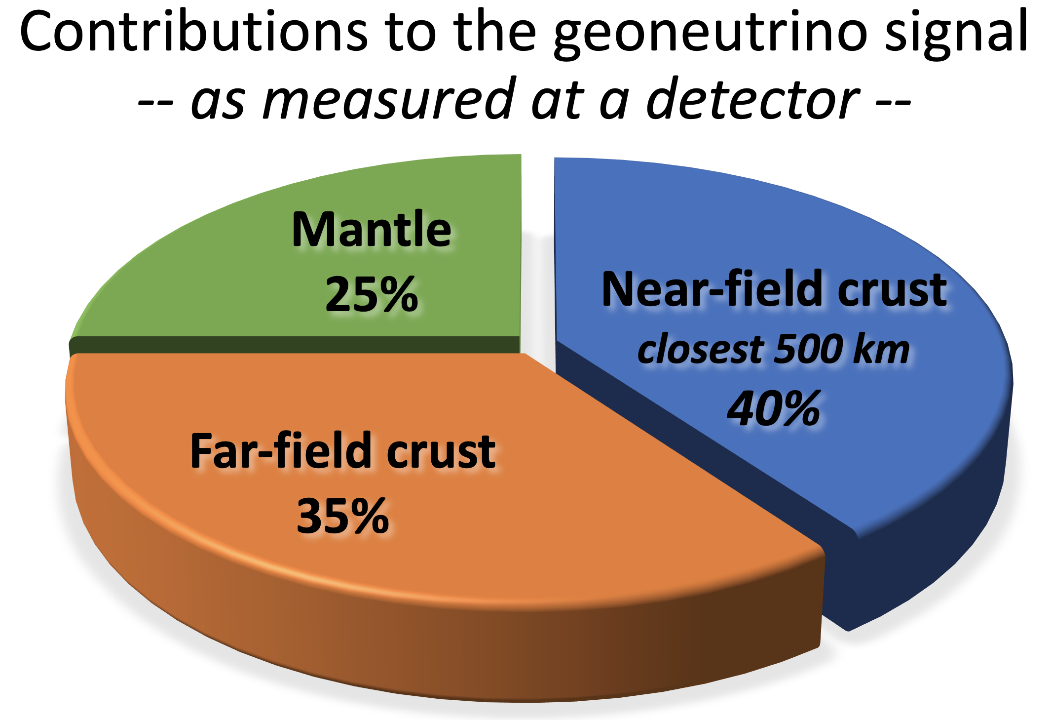
The total geoneutrino signal represents contributions of three components (Fig. 3): Near-field crust ( $\sim$ 40%), Far-field crust ( $\sim$ 35%, i.e., the global lithospheric signal), and Mantle signals ( $\sim$ 25%) [Wipperfurth2020]. Paramount in modeling the measured signal at a detector is understanding the contribution from the closest $\sim$ 500 km of lithosphere adjacent to the detector (i.e., 250 km outwards in any direction from the detector). This region is often referred to as the Near-field, local, or regional crustal signal. This part of the continental crust, and particularly the upper crust, is the region of greatest interest, because of the relative separation distance between source neutrino emitter and the detector, and because it is the brightest geoneutrino emitter due to geological processes that concentrate the HPEs upwards in the continental crust.

On average the continental crust is enriched in the HPE by more than a factor of 60 over the BSE and $>$ 100 over the present day abundances in the modern mantle. Moreover, the upper part of the crust is 10 times enriched in the HPE as compared to the lower crust [rudnickCompositionContinentalCrust2014, hackerContinentalLowerCrust2015a, Sammon2021, Wipperfurth2020]. Bulk compositional estimates of the continental crust report that it hosts about 30 to 40% of the heat producing elements in the BSE (Table 3).

Table 3: Heat producing elements in the continental crust

	Models of the continental crust $\|$				BSE model
citation ${}^{\dagger}$	1	2	2	3	4
Estimates of uncertainty	( $\pm$ 30%)	low	high	( $\pm$ 35%)	( $\pm$ 10%)
U ( $\mu$ g/g) in bulk Cont. crust	1.3	1.09	1.33	1.27	0.020
Th ( $\mu$ g/g) in bulk Cont. crust	5.6	4.20	5.31	5.64	0.077
K ( $\mu$ g/g) in bulk Cont. crust.	15000	11900	18800	11700	280
Heat production (nW/kg)	0.325	0.253	0.333	0.312	0.005
Heat production ( $\mu$ W/m ${}^{3}$ ) ${}^{*}$	0.943	0.733	0.967	0.906	0.023
Radiogenic power (TW) ${}^{\ddagger}$	7.2	5.7	7.4	7.1	20
% total U in CC	36%	30%	37%	36%	–
% total Th in CC	40%	30%	38%	40%	–
% total K in CC	29%	23%	37%	23%	–

${}^{\dagger}$ 1= [rudnickCompositionContinentalCrust2014], 2=[hackerContinentalLowerCrust2015a], 3=[Wipperfurth2020], and 4=[McDonough1995, Arevalo2009, wipperfurth:2018]. ${}^{*}$ assumes average $\rho$ (density) is 2900 kg/m ${}^{3}$ for the continental crust and 4450 kg/m ${}^{3}$ for the BSE. ${}^{\ddagger}$ see Table 1 for reservoir masses.

The estimated model compositions of the continental crust (Table 3) come with a considerable mount of uncertainty in their predicted abundances. Importantly, all of these models consider the upper crust to represent about the top third of the continent’s mass and assume a shared upper crustal compositional model [rudnickCompositionContinentalCrust2014], which dominates the geoneutrino flux. Using the global geophysical models that describe the continental crust (e.g., LITHO1.0) and a global model for the composition of the continents (Table 3), the geoneutrino signal for the Far-field crust (i.e., the crust minus the local contribution at the detector) ranges from $\sim$ 8 to 19 TNU, depending on the local setting [Wipperfurth2020]; locations like KamLAND and JUNO, near the coast, fall on the lower end of the scale, where as locations like Jinping and SNO+, surrounded by a significant amount of continental crust, fall on the high end of the range. \citeAWipperfurth2020 showed that when combining the data for KamLAND and Borexino and using their geological models, found a mantle signal of 9.2 $\pm$ 8.5 TNU and found the earth’s global radiogenic power to be 21.5 $\pm$ 10.4 TW.

The lithospheric signal can be treated globally, but the local lithospheric signal is best done with a detail analysis of the geological, geochemical, and geophysical data of the region. Using this combination of data one can build a 3D model of the chemical and physical attributes of the local lithosphere. It is noteworthy, however, that such attempts have been conducted at both the KamLAND and Borexino experiment locations. Figure 4 and Table 4 presents the range of predicted results for the geoneutrino flux at KamLAND, Borexino, and other locations.

7 Determining the radioactive power in the mantle

The particle physics experiment, at its simplest level, reports the geoneutrino flux at a detector. With this number in hand, along with a model for the local and global lithospheric contribution, the physicist then determines the planetary geoneutrino flux and the flux from the mantle. This idea was first laid out by \citeAKRAUSS. Later, \citeAraghavan1998measuring, in a comparative analyses of signals from detectors in continental and oceanic settings, specifically developed a scheme to determine the mantle flux.

Surface heat flux observations constrain the earth to radiating 46 $\pm$ 3 TW (i.e., 0.09 W/m ${}^{2}$ ). Based on a compositional model for the continental crust (Table 3), it contains about 7.1 ${}^{+2.1}_{-1.6}$ TW of radiogenic power, leaving $\sim$ 40 TW as a mantle flux contribution. This latter flux contains contributions from the core (basal heating), which is estimated to be order 10 $\pm$ 5 TW, and mantle (i.e., order 30 $\pm$ 5 TW, which includes radiogenic and primordial additions). A combined analysis of the KamLAND and Borexino results yields a mantle signal of 13 $\pm$ 12 TW [Wipperfurth2020]. Consequently, a large range of compositional models are acceptable for the earth’s radiogenic power (e.g., Table 4).

An important step towards reducing the uncertainties on the estimated mantle radiogenic power would be either (1) determine the mantle flux in oceanic setting and/or (2) improve the accuracy and precision of the local signal (Near-field). In the next section we address measuring the signal with an ocean bottom detector. Here we consider differences in estimates of the local signal.

Figure 4 and Table 4 illustrates the problem. The graph is designed to extract the mantle signal from the combined analysis of data from different detectors. The signal is made up of crust plus mantle; it is a two component only system (i.e., slope=1). The mantle signal (the ordinate intercept) can be considered, at this scale, homogeneous. Note, \citeASramek2013 found that even when modeling a mantle with 2 large, approximately antipodal structures (e.g., LLSVP: Large low shear velocity provinces), which might contain a factor of 5 or more difference in K, Th, and U abundances, the global mantle signal varied by only $\pm$ 10%. Thus, the mantle flux estimate highly depends on the accuracy of the crustal predictions for each detector.

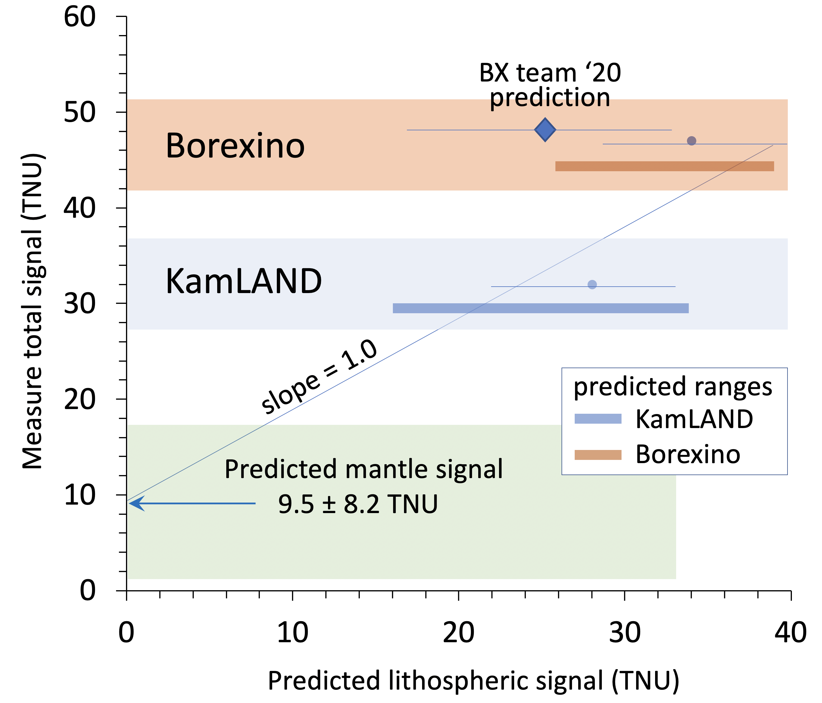
Figure 4 also reveals the challenge with different model predictions for the geoneutrino flux from the bulk lithosphere; each model and their uncertainties yields different geoneutrino flux estimates, and in turn this influences the prediction for the mantle signal. It is unclear which model provides a more accurate representation of the crust. In 2020, the Borexino particle physics team reported an updated prediction for the local lithospheric signal and mantle [agostini:2020], which lead to their distinctly higher prediction (and large uncertainty) for the earth’s total radiogenic power (i.e., 38 ${}^{+13.6}_{-12.7}$ TW). Thus, a clear challenge for the geological community is to independently construct a 3D model for the local lithosphere and from this predict a geoneutrino flux. By doing so, it would test this hypothesized lithospheric model constructed by the particle physics team and their markedly radiogenic prediction for the earth’s HPE abundances.

Table 4: Geological estimates of the signal contributions at various antineutrino detectors

Detector	reference	total	global crustal	FFC	NFC	$\dagger$ mantle
		signal	contribution			contribution
KamLAND	[enomoto2007neutrino]	38.5	28.2	10.5	17.7	10.3
KamLAND	[huang2013reference]	30.7	20.6	7.3	13.3	8.8
KamLAND	[fiorentini2012mantle]	–	26.5	8.8	17.7	–
KamLAND	[Wipperfurth2020]	37.9	27.0	8.8	18.2	9.4
Borexino	[huang2013reference]	43.5	29.0	13.7	15.3	8.7
Borexino	[coltorti2011u]	43.5	26.2	16.0	10.2	9.9
Borexino	[fiorentini2012mantle]	–	25.3	15.7	9.7	–
Borexino	[agostini:2020]	47.0	25.5	16.3	9.2	20.6
Borexino	[Wipperfurth2020]	43.9	32.5	14.8	18.2	9.4
SNO+	[huang2014regional]	40.0	30.7	15.1	15.6	7.0
SNO+	[strati2017perceiving]	43.1	30.5	15.2	15.3	6.9
SNO+	[Wipperfurth2020]	46.8	34.3	14.7	19.6	9.1
JUNO	[strati2015expected]	39.7	28.2	13.4	17.4	8.8
JUNO	[gao2020juloc]	49.1	38.3	9.8	28.5*	8.7
JUNO	[Wipperfurth2020]	40.5	29.8	12.7	17.1	9.5
Jinping	[sramek2016revealing]	58.5	50.3	16.1	27.2	8.2
Jinping	[Wan:Jinping]	59.4	49.0	–	–	10.4
Jinping	[Wipperfurth2020]	60.0	48.8	18.7	30.3	9.3
Hanohano	[huang2013reference]	12.0	2.6	2.6	–	9.0

All numbers are reported in units of TNU (see text for details). ${}^{\dagger}$ reported or calculated flux. NFF = Near Field Crust contribution, FFC = Far Field crust contribution, *authors defined the JUNO NFC as 10 ${}^{\circ}$ $\times$ 10 ${}^{\circ}$ . The flux contribution from the CLM (Continental Lithospheric Mantle) is not included, as it is not always reported by authors; it’s contribution is typically on the order of 1 to 2 TNU.