A new reduced order model of imcompressible Stokes equations

Abstract

In this paper we propose a new reduced order model (ROM) to the imcompressible Stokes equations. Numerical experiments show that our ROM is accurate and efficient. Under some assumptions on the problem data, we prove that the convergence rates of the new ROM is the same with standard solvers.

1 Introduction

Let $\Omega\subset\mathbb{R}^{d},d=2,3$, be a regular open domain with Lipschitz continuous boundary $\partial\Omega$. We consider the following imcompressible Stokes equation with no-slip boundary conditions:

$$u_{t}-\nu\Delta u+\nabla p =f\qquad\qquad\qquad\qquad\qquad\textup{ in }\Omega\times(0,T],$$ (1.1a)

$$\nabla\cdot u =0\qquad\qquad\qquad\qquad\qquad\textup{ in }\Omega\times(0,T],$$ (1.1b)

$$u =0\qquad\qquad\qquad\qquad\qquad\textup{ on }\partial\Omega\times(0,T],$$ (1.1c)

$$u(x,0) =u_{0}(x)\qquad\qquad\qquad\qquad\textup{ in }\Omega,$$ (1.1d)

where $u$ is the velocity, $p$ is the pressure, $f$ is the known body force, and $\nu$ is the viscosity.

In recent years, model order reduction (MOR) becomes more popular for solving partial differential equations (PDEs); see [16, 11, 13, 12, 1, 14, 15, 6, 10]. Especially, there has been a growing interest in the application of ROMs to modeling incompressible flows [9, 5]. These ROMs use experimental data, or solutions generated from full order model (FOM); however, when data is changed, there is no guarantee that the solution of the ROMs is accurate. In [17], we proposed a new ROM for the heat equation with changing data. We showed that the convergence rate of the new ROM is the same with the standard solvers, and the computational cost of the new ROM can be orders of magnitude smaller when compared to these full-order schemes.

Hence it is nature to ask, can we extend the idea in [17] to the Stokes equation?

In this paper we give a positive answer to the above question. First, we generate a sequence by solving a small number of time independent Stokes equations; see (3.1). Second, we solve two optimization problems to get reduced velocity and pressure spaces; see (P1) and (P2). The last step is to project the Stokes equation onto the reduced subspace, and obtain a velocity-only ROM; see (3.4). This is due to the fact that the reduced velocity space is weakly divergence free, and hence the pressure term was dropped out of the ROM formulation. To recover the pressure, we use the momentum equation recovery approach, which was proposed in [9, 6]. The numerical experiment in Example 3 shows that the new ROM is accurate and efficient. Furthermore, in Theorems 2 and 3 we prove that the convergence rates of the new ROM is the same with the standard solvers.

2 Notation and preliminaries

Throughout the paper, we assume $\Omega\subset\mathbb{R}^{d}$, $d=2,3$ is a bounded polyhedral domain. In order to give the weak form of the Stokes system (1.1) we need to introduce two function spaces $V$ and $Q$ for the velocity $u$ and pressure $p$, respectively. Let

$$V :=[H_{0}^{1}(\Omega)]^{d}=\left\{v\in[H^{1}(\Omega)]^{d}:\left.v\right|_{\partial\Omega}=0\right\},$$

$$Q :=L_{0}^{2}(\Omega)=\left\{q\in L^{2}(\Omega):\int_{\Omega}qdx=0\right\}.$$

We denote by $\|\cdot\|$ the $L^{2}(\Omega)$ norm and by $(\cdot,\cdot)$ the inner product, $\|\cdot\|_{V}$ the $V$ norm and by $(\cdot,\cdot)_{V}$ the inner product. For functions $v\in V$, the Poincaré inequality holds

$$\|v\|\leq C_{P}\|v\|_{V}.$$ (2.1)

Let $V^{\prime}$ be the dual space of bounded linear functionals defined on $V$, and let $\langle\cdot,\cdot\rangle_{V^{\prime},V}$ denotes the duality pairing between $V$ and its dual $V^{\prime}$. Then the space $V^{\prime}$ is equipped with the norm

$$\|f\|_{V^{\prime}}=\sup_{0\neq v\in V}\frac{\langle f,v\rangle_{V^{\prime},V}}{\|v\|_{V}}\quad\forall f\in V.$$

Now we can define the weak solution of (1.1): find $(u,p)\in V\times Q$ satisfying

$$\begin{split}\left(u_{t},v\right)+a(u,v)+b(v,p)&=(f,v)\qquad\qquad\qquad\qquad\forall v\in V,\\ b(u,q)&=0\qquad\qquad\qquad\qquad\qquad\forall q\in Q,\end{split}$$ (2.2)

where

$$a(u,v)=\nu(\nabla u,\nabla v),\quad b(u,q)=-(\nabla\cdot u,q).$$

For the above problem we know that the following inf-sup condition holds: there exists $\beta>0$ such that

$$\beta\leq\inf_{q\in Q}\sup_{v\in V}\frac{|b(v,q)|}{\|v\|_{V}\|q\|_{Q}}.$$ (2.3)

For any $(u,p)$, $(v,q)\in V\times Q$ we define

$$\mathscr{A}((u,p),(v,q))=a(u,v)+b(v,p)+b(u,q),\quad\textup{and}\;\;\|(v,q)\|_{V\times Q}^{2}=\|v\|_{V}^{2}+\|q\|_{Q}^{2}.$$

Lemma 1.

There exists a constant $C>0$ such that

$$\sup_{(v,q)\in V\times Q}\frac{\mathscr{A}((u,p),(v,q))}{\|(v,q)\|_{V\times Q}}\geq C\|(u,p)\|_{V\times Q}.$$ (2.4)

In order to formulate a numerical method, let $V_{h}$ and $Q_{h}$ be two spaces of piecewise polynomials that approximates $V$ and $Q$. Furthermore, we assume that the two finite element spaces $V_{h}$ and $Q_{h}$ satisfy the so-called discrete inf-sup condition: there exists $\beta_{h}>0$ such that

$$\beta_{h}\leq\inf_{q_{h}\in Q_{h}}\sup_{v_{h}\in V_{h}}\frac{|b(v_{h},q_{h})|}{\|v_{h}\|_{V}\|q_{h}\|_{Q}}.$$ (2.5)

Then the stability in Lemma 1 also holds on $V_{h}\times Q_{h}$.

The condition (2.5) is satisfied by several mixed finite elements, e.g., the Taylor-Hood elements and the MINI elements. In this paper, we shall use the Taylor-Hood elements for the numerical analysis and numerical experiments.

To simplify the presentation, we assume the initial condition $u_{0}=0$ and the source term $f$ does not depend on time. The semidiscrete finite element approximation of (2.2) takes the form: find $u_{h}(t)\in V_{h}$ with $u_{h}(0)=0$, and $p_{h}(t)\in Q_{h}$ such that

$$\begin{split}\left(\frac{{\rm d}}{{\rm d}t}u_{h},v_{h}\right)+a(u_{h},v_{h})+b(v_{h},p_{h})&=(f,v_{h})\qquad\qquad\qquad\qquad\forall v_{h}\in V_{h},\\ b(u_{h},q_{h})&=0\qquad\qquad\qquad\qquad\qquad\;\forall q_{h}\in Q_{h}.\end{split}$$ (2.6)

Next, we consider a discretization of the time interval $[0,T]$ into $N_{T}$ separate intervals such that $\Delta t=\frac{T}{N_{T}}$ and $t_{n}=n\Delta t$ for $n=0,\ldots,N_{T}$. We apply the backward Euler for the first step and then apply the two-steps backward differentiation formula (BDF2) for the time discretization. Specifically, given $u_{h}^{0}=0$, we find $u_{h}^{n}\in V_{h}$ and $p_{h}^{n}\in Q_{h}$ satisfying

$$\left(\partial_{t}^{+}u_{h}^{n},v_{h}\right)+a\left(u_{h}^{n},v_{h}\right)+b\left(v_{h},p_{h}^{n}\right) =\left(f,v_{h}\right)\qquad\;\;\forall v_{h}\in V_{h},$$ (2.7a)

$$b\left(u_{h}^{n},q_{h}\right) =0\qquad\qquad\quad\forall q_{h}\in Q_{h},$$ (2.7b)

where

$$\partial_{t}^{+}u_{h}^{n}=\begin{cases}\dfrac{u_{h}^{n}-u_{h}^{n-1}}{\Delta t},\qquad\qquad\quad\;n=1,\\[11.38092pt] \dfrac{3u_{h}^{n}-4u_{h}^{n-1}+u_{h}^{n-2}}{2\Delta t},\quad n\geq 2.\end{cases}$$

The computation can be extremely expensive if the mesh size $h$ and time step $\Delta t$ are small.

Example 1.

Let $\Omega=(0,1)\times(0,1)$ and $T=1$, we consider the Stokes equation (1.1) with

$$u_{0}=\left[\begin{array}[]{cccc}0\\[5.69046pt] 0\\ \end{array}\right],\quad f=\left[\begin{array}[]{cccc}f_{1}\\[5.69046pt] f_{2}\\ \end{array}\right],\quad f_{1}=100\sin(x)\exp(x),\quad f_{2}=100\cos(x)\exp(y).$$

We use $P_{2}-P_{1}$ Taylor-Hood element for spatial discretization and BDF2 for time discretization with time step $\Delta t=h^{3/2}$, here $h$ is the mesh size (max diameter of the triangles in the mesh). We report the wall time in Table 1.

$h$	$1/2^{1}$	$1/2^{2}$	$1/2^{3}$	$1/2^{4}$	$1/2^{5}$	$1/2^{6}$	$1/2^{7}$
Wall time	0.14	0.04	0.16	0.92	13.8	216	3851

Table 1: The wall time (seconds) for the simulation of Example 1.

3 Reduced order model (ROM)

For a given integer $\ell$ (small) and let $\mathfrak{u}_{h}^{0}=f$. For $1\leq i\leq\ell$, we find $\left(\mathfrak{u}_{h}^{i},\mathfrak{p}_{h}^{i}\right)\in V_{h}\times Q_{h}$ satisfying

$$\begin{split}a\left(\mathfrak{u}_{h}^{i},v_{h}\right)+b\left(v_{h},\mathfrak{p}_{h}^{i}\right)&=\left(\mathfrak{u}_{h}^{i-1},v_{h}\right)\qquad\qquad\qquad\forall v_{h}\in V_{h},\\ b\left(\mathfrak{u}_{h}^{i},q_{h}\right)&=0\qquad\qquad\qquad\qquad\qquad\forall q_{h}\in Q_{h}.\end{split}$$ (3.1)

Then, we consider the following minimization problems

$$\begin{split}\min_{{\widetilde{\varphi}}_{1},\ldots,{\widetilde{\varphi}}_{r_{u}}\in V_{h}}\sum_{j=1}^{\ell}\left\|\mathfrak{u}_{h}^{j}-\sum_{i=1}^{r_{u}}\left(\mathfrak{u}_{h}^{j},{\widetilde{\varphi}}_{i}\right)_{V}{\widetilde{\varphi}}_{i}\right\|_{V}^{2}\quad\text{ s.t. }\left({\widetilde{\varphi}}_{i},{\widetilde{\varphi}}_{j}\right)_{V}=\delta_{ij},1\leq i,j\leq r_{u},\end{split}$$ (P1)

and

$$\begin{split}\min_{{\widetilde{\psi}}_{1},\ldots,{\widetilde{\psi}}_{r_{p}}\in Q_{h}}\sum_{j=1}^{\ell}\left\|\mathfrak{p}_{h}^{j}-\sum_{i=1}^{r_{p}}\left(\mathfrak{p}_{h}^{j},{\widetilde{\psi}}_{i}\right){\widetilde{\psi}}_{i}\right\|^{2}\quad\text{ s.t. }\left({\widetilde{\psi}}_{i},{\widetilde{\psi}}_{j}\right)=\delta_{ij},1\leq i,j\leq r_{p}.\end{split}$$ (P2)

Let $\{\widetilde{\varphi}_{1},\widetilde{\varphi}_{2},\ldots,\widetilde{\varphi}_{r_{u}}\}$ and $\{\widetilde{\psi}_{1},\widetilde{\psi}_{2},\ldots,\widetilde{\psi}_{r_{p}}\}$ be the solution of (P1) and (P2), respectively. We define the reduced velocity space $V_{r}$ and pressure space $Q_{r}$ by

$$\begin{split}V_{r}=\textup{span}\{\widetilde{\varphi}_{1},\widetilde{\varphi}_{2},\ldots,\widetilde{\varphi}_{r_{u}}\},\qquad Q_{r}=\{\widetilde{\psi}_{1},\widetilde{\psi}_{2},\ldots,\widetilde{\psi}_{r_{p}}\}.\end{split}$$ (3.2)

One interesting property is that $V_{r}$ is weakly divergence free due to

$$V_{r}\subset\textup{span}\{\mathfrak{u}_{h}^{1},\mathfrak{u}_{h}^{2},\ldots,\mathfrak{u}_{h}^{\ell}\}\subset V_{h}^{\textup{div}}:=\left\{v_{h}\in V_{h},\quad b\left(v_{h},q_{h}\right)=0,\quad\forall q_{h}\in Q_{h}\right\}.$$ (3.3)

3.1 Velocity only ROM

Using the space $V_{r}$ we construct the BDF2-ROM scheme, given $u_{r}^{0}=0$, for each $n=1,2,\ldots,N_{T}$, we find velocity $u_{r}^{n}\in V_{r}$ satisfying

$$\left(\partial_{t}^{+}u_{r}^{n},v_{r}\right)+a\left(u_{r}^{n},v_{r}\right)=\left(f,v_{r}\right)\quad\forall v_{r}\in V_{r}.$$ (3.4)

The terms involving the pressure have dropped out of (3.4) due to (3.3).

3.2 Pressure recovery

The ROM (3.4) only computes the velocity. In this section, we use the velocity $u_{r}^{n},u_{r}^{n-1},u_{r}^{n-2}$ and the momentum equation (1.1a) to recover the pressure from the reduced pressure space $Q_{r}$. As we discussed in Section 3.1, the pressure was dropped from the formulation (3.4) due to $V_{r}\subset V_{h}^{\textup{div}}$. Hence, to recover the pressure, we need to use some test functions that do not belong to $V_{h}^{\textup{div}}$. From Hilbert space theory, the function space $V_{h}$ can be decomposed into the orthogonal subspaces:

$$V_{h}=V_{h}^{\textup{div}}\oplus\left(V_{h}^{\textup{div}}\right)^{\perp},$$

where the orthogonality is in the sense of the $V$ inner product.

The momentum equation recovery (MER) approach for recovering the pressure by using the weak form of the momentum equation via a Petrov-Galerkin projection, i.e., given the velocity only ROM solution $u_{r}^{n},u_{r}^{n-1},u_{r}^{n-2}$, determined by (3.4), find $p_{r}^{n}\in Q_{r}$ satisfying

$$b(s_{h},p_{r}^{n})=\left(f,s_{h}\right)-\left(\partial_{t}^{+}u_{r}^{n},s_{h}\right)-a\left(u_{r}^{n},s_{h}\right),\quad\forall s_{h}\in\mathcal{S}_{h}.$$ (3.5)

To recover the pressure $p_{r}^{n}$ from (3.5), we would require that the matrix form of $b(s_{h},p_{r}^{n})$ is square and invertible. In other words, we need to determine the test space $\mathcal{S}_{h}$ such that it is inf-sup stable with respect to the reduced pressure space $Q_{r}$. Following [9, 6], we consider the discrete inf-sup condition (2.5) by replacing the pressure finite element space with the ROM space $Q_{r}$:

$$\inf_{p_{r}\in Q_{r}\backslash\{0\}}\sup_{s_{h}\in\mathcal{S}_{h}\backslash\{0\}}\frac{b\left(s_{h},p_{r}\right)}{\left\|s_{h}\right\|_{V}\|p_{r}\|_{Q}}\geq\beta_{h}.$$ (3.6)

This can be done by using the Riesz representation in $V_{h}$ of the linear functional $b(\cdot,p_{r})$, i.e., find $s_{h}\in V_{h}$ such that

$$a\left(s_{h},v_{h}\right)=b\left(v_{h},p_{r}\right),\quad\forall v_{h}\in V_{h}.$$ (3.7)

Solving (3.7) for each basis function of $Q_{r}$ yields a set of basis functions $\left\{\zeta_{i}\right\}_{i=1}^{r_{p}}$. Letting

$$\mathcal{S}_{h}:=\operatorname{span}\left\{\zeta_{i}\right\}_{i=1}^{r_{p}}\subset\left(V_{h}^{\textup{div}}\right)^{\perp}\subset V_{h}.$$ (3.8)

We note that the test function $s_{h}\in\mathcal{S}_{h}\subset\left(V_{h}^{\textup{div}}\right)^{\perp}$ and the velocity solution $u_{r}^{n}\in V_{r}\subset V_{h}^{\textup{div}}$, then $a\left(u_{r}^{n},s_{h}\right)=0$. In other words, we find $p_{r}^{n}\in Q_{r}$ satisfying

$$b(s_{h},p_{r}^{n})=\left(f,s_{h}\right)-\left(\partial_{t}^{+}u_{r}^{n},s_{h}\right),\quad\forall s_{h}\in\mathcal{S}_{h}.$$ (3.9)

3.3 Implementation

First, we compute $\left(\mathfrak{u}_{h}^{i},\mathfrak{p}_{h}^{i}\right)$ by solving (3.1). Let $\mathcal{P}^{k}(K)$ denote the set of polynomials of degree at most $k$ on an element $K$. We define

$$V_{h} =\left\{v_{h}\in C(\bar{\Omega})\big{|}v_{h}|_{K}\in\mathcal{P}^{k+1}(K)\right\}=\operatorname{span}\left\{\varphi_{1},\ldots,\varphi_{N_{u}}\right\},$$

$$Q_{h} =\left\{q_{h}\in C(\bar{\Omega})\big{|}q_{h}|_{K}\in\mathcal{P}^{k}(K)\right\}=\operatorname{span}\left\{\psi_{1},\ldots,\psi_{N_{p}}\right\}.$$

Define

$$M_{ij}=(\varphi_{j},\varphi_{i}),\quad A_{ij}=a(\varphi_{j},\varphi_{i}),\quad B_{ij}=b(\varphi_{j},\psi_{i}),\quad W_{ij}=(\psi_{j},\psi_{i}),\quad b_{i}=(f,\varphi_{i}).$$ (3.10)

Let $\texttt{u}_{i}$ and $\texttt{p}_{i}$ be the coefficients of $\mathfrak{u}_{h}^{i}$ and $\mathfrak{p}_{h}^{i}$, $1\leq i\leq\ell$, i.e.,

$$\mathfrak{u}_{h}^{i}=\sum_{j=1}^{N_{u}}\left(\texttt{u}_{i}\right)_{j}\varphi_{j},\qquad\textup{and}\qquad\mathfrak{p}_{h}^{i}=\sum_{j=1}^{N_{p}}\left(\texttt{p}_{i}\right)_{j}\psi_{j},$$ (3.11)

where $(\alpha)_{j}$ denotes the $j$-th component of the vector $\alpha$. Then substitute (3.11) into (3.1) we obtain

$$\left[\begin{array}[]{cccc}A&B\\[5.69046pt] -B^{\top}&O\\ \end{array}\right]\left[\begin{array}[]{cccc}\texttt{u}_{1}\\[5.69046pt] \texttt{p}_{1}\\ \end{array}\right]=\left[\begin{array}[]{cccc}b\\[5.69046pt] O\\ \end{array}\right],\qquad\left[\begin{array}[]{cccc}A&B\\[5.69046pt] -B^{\top}&O\\ \end{array}\right]\left[\begin{array}[]{cccc}\texttt{u}_{i}\\[5.69046pt] \texttt{p}_{i}\\ \end{array}\right]=\left[\begin{array}[]{cccc}M\texttt{u}_{i-1}\\[5.69046pt] O\\ \end{array}\right],\qquad 2\leq i\leq\ell,$$ (3.24)

The algebraic system (3.24) has defects. One of which is that the matrix is singular so that solving (3.24) is usually impossible. There are two common ways to treat this issue, the first one is to fix the pressure at one point and the second is to impose zero mean by introducing a Lagrange multiplier. In this paper, we shall use the first approach.

After we solved (3.1), we collect the coefficients of $\mathfrak{u}_{h}^{i}$ and $\mathfrak{p}_{h}^{i}$. Define the matrices $U_{\ell}$ and $P_{\ell}$ by

$$U_{\ell}=[\texttt{u}_{1}\mid\texttt{u}_{2}\mid\ldots\mid\texttt{u}_{\ell}]\in\mathbb{R}^{N_{u}\times\ell},\qquad P_{\ell}=[\texttt{p}_{1}\mid\texttt{p}_{2}\mid\ldots\mid\texttt{p}_{\ell}]\in\mathbb{R}^{N_{p}\times\ell}.$$ (3.25)

Next, we shall solve the optimization problems (P1) and (P2) to find the reduced velocity and pressure space. The approach taken is the same as in [17], hence we only list the essential steps.

• Let

  $$K_{\ell}=U_{\ell}^{\top}AU_{\ell},\qquad G_{\ell}=P_{\ell}^{\top}WP_{\ell}.$$ (3.26)

• Let $\lambda_{k}(K_{\ell})$ and $x_{k}$ be the $k$-th eigenvalue and eigenvector of $K_{\ell}$; $\lambda_{k}(G_{\ell})$ and $y_{k}$ be the $k$-th eigenvalue and eigenvector of $G_{\ell}$.

• Give a tolerance tol, we find the minimal $r_{u}$ and $r_{p}$ such that

  $$\dfrac{\sum_{k=1}^{r_{u}}\lambda_{k}(K_{\ell})}{\sum_{k=1}^{\ell}\lambda_{k}(K_{\ell})}\geq 1-\texttt{tol},\qquad\dfrac{\sum_{k=1}^{r_{p}}\lambda_{k}(G_{\ell})}{\sum_{k=1}^{\ell}\lambda_{k}(G_{\ell})}\geq 1-\texttt{tol}.$$

• Let $\widetilde{x}_{k}=\frac{1}{\sqrt{\lambda_{k}(K_{\ell})}}U_{\ell}x_{k}$, $k=1,2\ldots,r_{u}$; $\widetilde{y}_{k}=\frac{1}{\sqrt{\lambda_{k}(G_{\ell})}}P_{\ell}y_{k}$, $k=1,2\ldots,r_{p}$. We note that $\widetilde{x}_{k}$ and $\widetilde{y}_{k}$ are the coefficients of $\widetilde{\varphi}_{k}$ and $\widetilde{\psi}_{k}$, respectively.

• Define $Q_{u}=[\widetilde{x}_{1}\mid\widetilde{x}_{2}\mid\cdots\mid\widetilde{x}_{r_{u}}]$ and $Q_{p}=[\widetilde{y}_{1}\mid\widetilde{y}_{2}\mid\cdots\mid\widetilde{y}_{r_{p}}]$. Therefore,

  $$\begin{split}Q_{u}&=U_{\ell}[x_{1}\mid x_{2}\mid\ldots|x_{r_{u}}]\begin{bmatrix}\frac{1}{\sqrt{\lambda_{1}(K_{\ell})}}&&\\ &\ddots&\\ &&\frac{1}{\sqrt{\lambda_{r_{u}}(K_{\ell})}}\end{bmatrix}\in\mathbb{R}^{N_{u}\times r_{u}},\\ Q_{p}&=P_{\ell}[y_{1}\mid y_{2}\mid\ldots|y_{r_{p}}]\begin{bmatrix}\frac{1}{\sqrt{\lambda_{1}(G_{\ell})}}&&\\ &\ddots&\\ &&\frac{1}{\sqrt{\lambda_{r_{p}}(G_{\ell})}}\end{bmatrix}\in\mathbb{R}^{N_{p}\times r_{p}}.\end{split}$$ (3.27)

Once we obtained the reduced pressure space, we then compute the basis of $\mathcal{S}_{h}$. In other words, we solve (3.7) with $p_{r}=\widetilde{\psi}_{j}$. Assume that $s_{j,h}\in V_{h}$ is the solution, $1\leq j\leq r_{p}$, and let $s_{j}$ be the coefficient of $s_{j,h}$ under the finite element basis $\{\varphi_{k}\}_{k=1}^{N_{u}}$, i.e., $s_{j,h}=\sum_{k=1}^{N_{u}}(s_{j})_{k}\varphi_{k}$, $1\leq j\leq r_{p}$. Then the matrix equation of (3.7) is

$$A\underbrace{\left[s_{1}~{}\big{|}~{}s_{2}~{}\big{|}\cdots\big{|}s_{r_{p}}\right]}_{S}=BQ_{p}.$$

Then the reduced velocity space $V_{r}$, the reduced pressure spaces $Q_{r}$, and the space $\mathcal{S}_{h}$ are defined by

$$V_{r} =\textup{span}\{\widetilde{\varphi}_{1},\widetilde{\varphi}_{2},\ldots,\widetilde{\varphi}_{r_{u}}\},\qquad\;\textup{with}\;\;\widetilde{\varphi}_{k}=\sum_{j=1}^{r_{u}}Q_{u}(j,k)\varphi_{j},$$

$$Q_{r} =\textup{span}\{\widetilde{\psi}_{1},\widetilde{\psi}_{2},\ldots,\widetilde{\psi}_{r_{u}}\},\qquad\;\textup{with}\;\;\widetilde{\varphi}_{k}=\sum_{j=1}^{r_{p}}Q_{p}(j,k)\psi_{j},$$

$$\mathcal{S}_{h} =\textup{span}\{s_{1,h},s_{2,h},\ldots,s_{r_{p},h}\},\quad\textup{with}\;\;s_{k,h}=\sum_{j=1}^{r_{u}}S(j,k)\varphi_{j}.$$

The next step is to give the matrix form of (3.4) and (3.9). Since $u_{r}^{n}\in V_{r}$ and $p_{r}^{n}\in Q_{r}$ hold, we then make the Galerkin ansatz of the form

$$u_{r}^{n}=\sum_{j=1}^{r_{u}}\left(\alpha_{r}^{n}\right)_{j}{\widetilde{\varphi}}_{j},\qquad p_{r}^{n}=\sum_{j=1}^{r_{p}}\left(\beta_{r}^{n}\right)_{j}{\widetilde{\psi}}_{j}.$$ (3.28)

We insert (3.28) into (3.4) and (3.9) to obtain the following linear matrix form:

$$\begin{split}M_{r}\partial_{t}^{+}\alpha_{r}^{n}+A_{r}\alpha_{r}^{n}=b_{r},\quad\alpha_{r}^{0}=0,\\ B_{r}\beta_{r}^{n}=\widetilde{b}_{r}-W_{r}\partial_{t}^{+}\alpha_{r}^{n},\end{split}$$ (3.29)

where

$$M_{r}=Q_{u}^{\top}MQ_{u}\in\mathbb{R}^{r_{u}\times r_{u}},\qquad A_{r}=Q_{u}^{\top}AQ_{u}\in\mathbb{R}^{r_{u}\times r_{u}},\qquad b_{r}=Q_{u}^{\top}b\in\mathbb{R}^{r_{u}},$$

$$B_{r}=S^{\top}BQ_{p}\in\mathbb{R}^{r_{p}\times r_{p}},\qquad W_{r}=(BQ_{p})^{\top}MQ_{u}\in\mathbb{R}^{r_{p}\times r_{u}},\qquad\widetilde{b}_{r}=S^{\top}b\in\mathbb{R}^{r_{p}}.$$

The final step is to return the solution of the ROM to the FOM. In other words, we shall express the solutions $u_{r}^{n}$ and $p_{r}^{n}$ under the finite element basis functions. By (3.28) and (3.27) we have

$$u_{r}^{n}=\sum_{j=1}^{r_{u}}\left(\alpha_{r}^{n}\right)_{j}{\widetilde{\varphi}}_{j}=\sum_{j=1}^{r_{u}}\left(\alpha_{r}^{n}\right)_{j}\sum_{i=1}^{N_{u}}(\widetilde{x}_{j})_{i}\varphi_{i}=\sum_{i=1}^{N_{u}}(Q_{u}\alpha_{r}^{n})_{i}\varphi_{i},$$

$$p_{r}^{n}=\sum_{j=1}^{r_{p}}\left(\beta_{r}^{n}\right)_{j}{\widetilde{\psi}}_{j}=\sum_{j=1}^{r_{p}}\left(\beta_{r}^{n}\right)_{j}\sum_{i=1}^{N_{p}}(\widetilde{y}_{j})_{i}\psi_{i}=\sum_{i=1}^{N_{p}}(Q_{p}\beta_{r}^{n})_{i}\psi_{i}.$$

That is to say, the solution $u_{r}^{n}$, in terms of the finite element basis $\left\{\varphi_{1},\ldots,\varphi_{N_{u}}\right\}$, the coefficient is $Q_{u}\alpha_{r}^{n}$; the solution $p_{r}^{n}$, in terms of the finite element basis $\left\{\psi_{1},\ldots,\varphi_{N_{p}}\right\}$, the coefficient is $Q_{p}\beta_{r}^{n}$.

Now, we summarize the above discussions in Algorithm 1.

Algorithm 1

Input: tol, $\ell$, $M$, $W$, $A$, $B$, $b$

1:Solve $\left[\begin{array}[]{cccc}A&B\\[5.69046pt] -B^{\top}&O\\ \end{array}\right]\left[\begin{array}[]{cccc}\texttt{u}_{1}\\[5.69046pt] \texttt{p}_{1}\\ \end{array}\right]=\left[\begin{array}[]{cccc}b\\[5.69046pt] O\\ \end{array}\right]$;

2:for $i=2$ to $\ell$ do

3:     Solve $\left[\begin{array}[]{cccc}A&B\\[5.69046pt] -B^{\top}&O\\ \end{array}\right]\left[\begin{array}[]{cccc}\texttt{u}_{i}\\[5.69046pt] \texttt{p}_{i}\\ \end{array}\right]=\left[\begin{array}[]{cccc}M\texttt{u}_{i-1}\\[5.69046pt] O\\ \end{array}\right]$;

4:end for

5:Set $U=[\texttt{u}_{1}\mid\texttt{u}_{2}\mid\ldots\mid\texttt{u}_{\ell}]$; $P=[\texttt{p}_{1}\mid\texttt{p}_{2}\mid\ldots\mid\texttt{p}_{\ell}]$;

6:Set $K=U^{\top}AU$;  $[X,\Lambda_{1}]=\textup{eig}(K)$;  $G=P^{\top}WP$; $[Y,\Lambda_{2}]=\textup{eig}(G)$;

7:Find minimal $r_{u}$ and $r_{p}$ such that $\frac{\sum_{i=1}^{r_{u}}\Lambda_{1}(i,i)}{\sum_{i=1}^{\ell}\Lambda_{1}(i,i)}\geq 1-\texttt{tol}$ and $\frac{\sum_{i=1}^{r_{p}}\Lambda_{2}(i,i)}{\sum_{i=1}^{\ell}\Lambda_{2}(i,i)}\geq 1-\texttt{tol}$ .

8:Set $Q_{u}=UX(:,1:r_{u})(\Lambda_{1}(1:r_{u},1:r_{u}))^{-1/2}$ and $Q_{p}=PY(:,1:r_{p})(\Lambda_{2}(1:r_{p},1:r_{p}))^{-1/2}$;

9:Solve $AS=BQ_{p}$;

10:Set $M_{r}=Q_{u}^{\top}MQ_{u}$; $A_{r}=Q_{u}^{\top}AQ_{u}$; $b_{r}=Q_{u}^{\top}b$; $B_{r}=S^{\top}BQ_{p}$; $W_{r}=(BQ_{p})^{\top}MQ_{u}$; $\widetilde{b}_{r}=S^{\top}b$;

11:for $n=1$ to $N_{T}$ do

12:     Solve $M_{r}\partial_{t}^{+}\alpha_{r}^{n}+A_{r}\alpha_{r}^{n}=b_{r}$;

13:     Solve $B_{r}\beta_{r}^{n}=\widetilde{b}_{r}-W_{r}\partial_{t}^{+}\alpha_{r}^{n}$;

14:end for

15:return $Q_{u}$, $Q_{p}$, $\{\alpha_{r}^{n}\}_{n=1}^{N_{T}}$, $\{\beta_{r}^{n}\}_{n=1}^{N_{T}}$

4 Theoretical analysis

It seems that the dimension of the reduced velocity space $V_{r}$ and pressure space $Q_{r}$ depends on the eigenvalues of $K_{\ell}$ and $G_{\ell}$, respectively. However, in this section we prove that only the eigenvalues of $K_{\ell}$ determine the main computational cost and the dimension of $V_{r}$ and $Q_{r}$. Furthermore, we show that the eigenvalues of $K_{\ell}$ are exponentially decay.

Our discussion relies on the discrete eigenvalue problem of the Stokes equation. Let $(\phi_{h},\chi_{h},\lambda_{h})$, with $\phi_{h}\neq 0$ and $\lambda_{h}\in\mathbb{R}$ be the solution of

$$a(\phi_{h},v_{h})+b(v_{h},\chi_{h}) =\lambda_{h}(\phi_{h},v_{h})\qquad\qquad\qquad\quad\forall v_{h}\in V_{h},$$ (4.1a)

$$b(\phi_{h},q_{h}) =0\qquad\qquad\qquad\qquad\qquad\;\;\;\forall q_{h}\in Q_{h}.$$ (4.1b)

It is well known that the discrete Stokes eigenvalue problem (4.1) has a finite sequence of eigenvalues and eigenfunctions

$$0<\lambda_{1,h}\leq\lambda_{2,h}\leq\ldots\leq\lambda_{N_{u},h},\quad\left(\phi_{1,h},\chi_{1,h}\right),\left(\phi_{2,h},\chi_{2,h}\right),\ldots,\left(\phi_{N_{u},h},\chi_{N_{u},h}\right),\quad(\phi_{i,h},\phi_{j,h})_{V}=\delta_{ij}.$$

Define $\mathcal{A}_{h}:V_{h}\times Q_{h}\to V_{h}\times Q_{h}$ by

$$\mathscr{A}((u_{h},p_{h}),(v_{h},q_{h}))=\left(\mathcal{A}_{h}(u_{h},p_{h}),(v_{h},q_{h})\right)\quad\text{ for all }(v_{h},q_{h})\in V_{h}\times Q_{h}.$$ (4.2)

It is easy to verify that $\mathcal{A}_{h}^{-1}:V_{h}\times Q_{h}\to V_{h}\times Q_{h}$ exists, and

$$\mathcal{A}_{h}^{-1}\left[\begin{array}[]{cc}\phi_{i,h}\\[5.69046pt] 0\end{array}\right]=\lambda_{i,h}^{-1}\left[\begin{array}[]{cc}\phi_{i,h}\\[5.69046pt] \chi_{i,h}\end{array}\right].$$ (4.7)

By the definition of $\left(\mathfrak{u}_{h}^{1},\mathfrak{p}_{h}^{1}\right)$ in (3.1), for all $(v_{h},q_{h})\in V_{h}\times Q_{h}$ we have

$$\left(\mathcal{A}_{h}(\mathfrak{u}_{h}^{1},\mathfrak{p}_{h}^{1}),(v_{h},q_{h})\right)=((f,0),(v_{h},q_{h}))=((\Pi f,0),(v_{h},q_{h})),$$ (4.8)

where $\Pi:[L^{2}(\Omega)]^{d}\to V_{h}$ be the standard $L^{2}$ projection. Therefore

$$\left[\begin{array}[]{cc}\mathfrak{u}_{h}^{1}\\[5.69046pt] \mathfrak{p}_{h}^{1}\end{array}\right]=\mathcal{A}_{h}^{-1}\left[\begin{array}[]{cc}\Pi f\\[5.69046pt] 0\end{array}\right].$$ (4.13)

For $i=2,3\ldots,\ell$, we have

$$\left[\begin{array}[]{cc}\mathfrak{u}_{h}^{i}\\[5.69046pt] \mathfrak{p}_{h}^{i}\end{array}\right]=\mathcal{A}_{h}^{-1}\left[\begin{array}[]{cc}\mathfrak{u}_{h}^{i-1}\\[5.69046pt] 0\end{array}\right].$$ (4.18)

Obviously, $\{\left(\mathfrak{u}_{h}^{1},\mathfrak{p}_{h}^{1}\right),\left(\mathfrak{u}_{h}^{2},\mathfrak{p}_{h}^{2}\right),\ldots,\left(\mathfrak{u}_{h}^{\ell},\mathfrak{p}_{h}^{\ell}\right)\}$ is not a Krylov sequence. However, we can show that $\{\mathfrak{u}_{h}^{1},\mathfrak{u}_{h}^{2},\ldots,\mathfrak{u}_{h}^{\ell}\}$ is a Krylov sequence.

Lemma 2.

The sequence $\{\mathfrak{u}_{h}^{1},\mathfrak{u}_{h}^{2},\ldots,\mathfrak{u}_{h}^{\ell}\}$ is a Krylov sequence.

Proof.

Let $f_{h}$ be the standard $L^{2}$ projection of $f$ in $V_{h}$ and assume that

$$f_{h}=\sum_{j=1}^{N_{u}}c_{j}\phi_{j,h}.$$

By (4.7) and (4.13) we have

$$\left[\begin{array}[]{cc}\mathfrak{u}_{h}^{1}\\[5.69046pt] \mathfrak{p}_{h}^{1}\end{array}\right]=\mathcal{A}_{h}^{-1}\left[\begin{array}[]{cc}\Pi f\\[5.69046pt] 0\end{array}\right]=\mathcal{A}_{h}^{-1}\left[\begin{array}[]{cc}\displaystyle\sum_{i=1}^{N_{u}}c_{i}\phi_{i,h}\\[11.38092pt] 0\end{array}\right]=\sum_{i=1}^{N_{u}}c_{i}\lambda_{i,h}^{-1}\left[\begin{array}[]{cc}\phi_{i,h}\\[11.38092pt] \chi_{i,h}\end{array}\right].$$

By the same argument as above, we formally have

$$\left[\begin{array}[]{cc}\left(\mathfrak{u}_{h}^{1},\mathfrak{p}_{h}^{1}\right)\\[8.5359pt] \left(\mathfrak{u}_{h}^{2},\mathfrak{p}_{h}^{2}\right)\\ \vdots\\ \left(\mathfrak{u}_{h}^{\ell},\mathfrak{p}_{h}^{\ell}\right)\end{array}\right]=\left[\begin{array}[]{cccc}c_{1}\mu_{1}&c_{2}\mu_{2}&\cdots&c_{N_{u}}\mu_{N_{u}}\\[5.69046pt] c_{1}\mu_{1}^{2}&c_{2}\mu_{2}^{2}&\cdots&c_{N_{u}}\mu_{N_{u}}^{2}\\[5.69046pt] \vdots&\vdots&\cdots&\vdots\\ c_{1}\mu_{1}^{\ell}&c_{2}\mu_{2}^{\ell}&\cdots&c_{N_{u}}\mu_{N_{u}}^{\ell}\\[5.69046pt] \end{array}\right]\left[\begin{array}[]{cc}(\phi_{1,h},\chi_{1,h})\\[5.69046pt] (\phi_{2,h},\chi_{2,h})\\ \vdots\\ (\phi_{N_{u},h},\chi_{N_{u},h})\end{array}\right].$$ (4.31)

We define $\mathscr{B}_{h}:V_{h}\to V_{h}$ by

$$\mathscr{B}_{h}v_{h}=\sum_{j=1}^{N_{u}}\mu_{j}(v_{h},\phi_{j,h})_{V}\phi_{j,h}.$$ (4.32)

It is easy to show that $\mathscr{B}_{h}:V_{h}\to V_{h}$ is bounded with the $V$-norm, then

$$\{\mathfrak{u}_{h}^{1},\mathfrak{u}_{h}^{2},\ldots,\mathfrak{u}_{h}^{\ell}\}=\{\mathscr{B}_{h}f_{h},\mathscr{B}_{h}^{2}f_{h},\ldots,\mathscr{B}_{h}^{\ell}f_{h}\}.$$

∎

For each $\mathfrak{u}_{h}^{i-1}\in V_{h}$, we can determine $\mathfrak{p}_{h}^{i}\in Q_{h}$ by (4.18), this determines a linear operator $\mathscr{C}_{h}:V_{h}\to Q_{h}$ by

$$\mathfrak{p}_{h}^{i}=\mathscr{C}_{h}\mathfrak{u}_{h}^{i-1},\quad i=1,2,\ldots,\ell.$$

This implies

$$\{\mathfrak{p}_{h}^{1},\mathfrak{p}_{h}^{2},\ldots,\mathfrak{p}_{h}^{\ell}\}=\{\mathscr{C}_{h}\mathscr{B}_{h}f_{h},\mathscr{C}_{h}\mathscr{B}_{h}^{2}f_{h},\ldots,\mathscr{C}_{h}\mathscr{B}_{h}^{\ell}f_{h}\}.$$ (4.33)

Remark 1.

The sequence $\{\mathfrak{p}_{h}^{1},\mathfrak{p}_{h}^{2},\ldots,\mathfrak{p}_{h}^{\ell}\}$ is not a Krylov sequence.

Let $r\leq\ell$ be the largest number such that $\{\mathfrak{u}_{h}^{1},\mathfrak{u}_{h}^{2},\ldots,\mathfrak{u}_{h}^{r}\}$ is linear independent. Although $\{\mathfrak{p}_{h}^{1},\mathfrak{p}_{h}^{2},\ldots,\mathfrak{p}_{h}^{\ell}\}$ is not a Krylov sequence, by (4.33) we know that

$$\textup{span}\{\mathfrak{p}_{h}^{1},\mathfrak{p}_{h}^{2},\ldots,\mathfrak{p}_{h}^{r}\}=\textup{span}\{\mathfrak{p}_{h}^{1},\mathfrak{p}_{h}^{2},\ldots,\mathfrak{p}_{h}^{r},\ldots\}.$$

This implies that the dimension of $Q_{r}$ is no larger than $r$. In other words, the eigenvalues of $K_{\ell}$ determine not only the dimension of $V_{r}$, but also the up-bound dimension of $Q_{r}$.

Furthermore, the matrices $K_{j}$, $j=1,2\ldots,r$ are positive definite and $K_{r+1}$ is positive semi-definite. Hence, we only to compute the minimal eigenvalue of the matrices $K_{1},K_{2},\ldots$. Once the minimal eigenvalue of some matrix is zero, we then stop.

In practice, we terminate the process if the minimal eigenvalue of some matrix is small.

Following the same arguments in [17], we can prove that the matrices $K_{\ell}$ in (3.26) is Hankel type matrix, i.e., each ascending skew-diagonal from left to right is constant. Therefore, to assemble the matrix $K_{r}$, we only need the matrix $K_{r-1}$ and to compute $\texttt{u}_{r-1}^{\top}A\texttt{u}_{r}$ and $\texttt{u}_{r}^{\top}A\texttt{u}_{r}$. Next we summarize the above discussion in Algorithm 2.

Algorithm 2 (Get $Q_{u}$ and $Q_{p}$)

Input: tol, $\ell$, $M$, $W$, $A$, $B$, $b$

1:Solve $\left[\begin{array}[]{cccc}A&B\\[5.69046pt] -B^{\top}&O\\ \end{array}\right]\left[\begin{array}[]{cccc}\texttt{u}_{1}\\[5.69046pt] \texttt{p}_{1}\\ \end{array}\right]=\left[\begin{array}[]{cccc}b\\[5.69046pt] O\\ \end{array}\right]$;

2:Let $K_{1}=\texttt{u}_{1}^{\top}A\texttt{u}_{1}$;

3:for $i=2$ to $\ell$ do

4:     Solve $\left[\begin{array}[]{cccc}A&B\\[5.69046pt] -B^{\top}&O\\ \end{array}\right]\left[\begin{array}[]{cccc}\texttt{u}_{i}\\[5.69046pt] \texttt{p}_{i}\\ \end{array}\right]=\left[\begin{array}[]{cccc}M\texttt{u}_{i-1}\\[5.69046pt] O\\ \end{array}\right]$;

5:     Get $\alpha=[K_{i-1}(i-1,2:i-1)\mid\texttt{u}_{i-1}^{\top}A\texttt{u}_{i}]$ and $\beta=\texttt{u}_{i}^{\top}A\texttt{u}_{i}$;

6:     $K_{i}=\left[\begin{array}[]{cc}K_{i-1}&\alpha^{\top}\\ \alpha&\beta\\ \end{array}\right]$;

7:     $[X,\Lambda_{1}]=\textup{eig}(K_{i})$;

8:     if $\Lambda_{1}(i,i)\leq\textup{tol}$ then

9:         break;

10:     end if

11:end for

12:Set $U=[\texttt{u}_{1}\mid\texttt{u}_{2}\mid\ldots\mid\texttt{u}_{i}]$; $P=[\texttt{p}_{1}\mid\texttt{p}_{2}\mid\ldots\mid\texttt{p}_{i-1}]$;

13:Set $G=P^{\top}WP$; $[Y,\Lambda_{2}]=\textup{eig}(G)$;

14:Find minimal $r_{p}$ such that $\frac{\sum_{j=1}^{r_{p}}\Lambda_{2}(j,j)}{\sum_{j=1}^{i-1}\Lambda_{2}(j,j)}\geq 1-\textup{tol}$;

15:Set $Q_{p}=PY(:,1:r_{p})(\Lambda_{2}(1:r_{p},1:r_{p}))^{-1/2}$;

16:Set $Q_{u}=UX(:,1:i-1)(\Lambda_{1}(1:i-1,1:i-1))^{-1/2}$;

17:return $Q_{u},Q_{p}$

Next, we give the estimation of the eigenvlaues of $K_{r}$. The proof of the following Theorem 1 is the same with the proof of [17], hence we omit the details here.

Theorem 1.

Let $\lambda_{1}({K_{r}})\geq\lambda_{2}({K_{r}})\geq\ldots\geq\lambda_{r}({K_{r}})>0$ be the eigenvalues of $K_{r}$, then

$$\lambda_{2k+1}({K_{r}})\leq 16\left[\exp\left(\frac{\pi^{2}}{4\log(8\lfloor r/2\rfloor/\pi)}\right)\right]^{-2k+2}\lambda_{1}({K_{r}}),\qquad 2k+1\leq r.$$ (4.34)

Moreover, the minimal eigenvalue of $K_{r}$ satisfies

$$\lambda_{\min}({K_{r}})\leq C(2r-1)\|f\|_{V^{\prime}}^{2}\exp\left(-\dfrac{7(r+1)}{2}\right).$$ (4.35)

Example 2.

We use the same problem data as in the Example 1 and take $h=1/100$. We report all the eigenvalues of $K_{10}$ and $G_{10}$ in Figure 1. It is clear that the eigenvalues of both $K_{10}$ and $G_{10}$ are exponentially decay. This matches our theoretical result in Theorem 1.

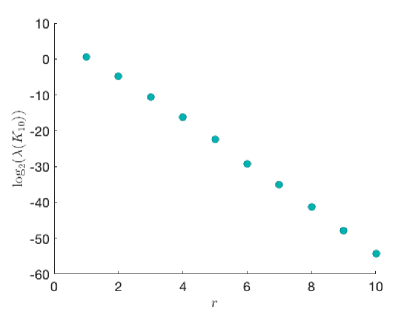
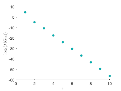
Figure 1: The eigenvalues of the matrices $K_{10}$ and $G_{10}$.

Finally, we give the full implementation of Equation 3.4.

Algorithm 3

Input: tol, $\ell$, $N_{T}$, $\Delta t$, $M$, $W$, $A$, $B$, $b$

1:$[Q_{u},Q_{p}]=\texttt{GetQuQp}(\textup{tol},\ell,M,W,A,B,b)$;                                                      % Algorithm 2

2:Solve $AS=BQ_{p}$;

3:Set $M_{r}=Q_{u}^{\top}MQ_{u}$; $A_{r}=Q_{u}^{\top}AQ_{u}$; $b_{r}=Q_{u}^{\top}b$; $B_{r}=S^{\top}AS$; $W_{r}=(BQ_{p})^{\top}MQ_{u}$; $\widetilde{b}_{r}=S^{\top}b$;

4:for $n=1$ to $N_{T}$ do

5:     Solve $M_{r}\partial_{t}^{+}\alpha_{r}^{n}+A_{r}\alpha_{r}^{n}=b_{r}$;

6:     Solve $B_{r}\beta_{r}^{n}=\widetilde{b}_{r}-W_{r}\partial_{t}^{+}\alpha_{r}^{n}$;

7:end for

8:return $Q_{u}$, $Q_{p}$, $\{\alpha_{r}^{n}\}_{n=1}^{N_{T}}$, $\{\beta_{r}^{n}\}_{n=1}^{N_{T}}$

Example 3.

We revisit the Example 1 under the same problem data, mesh and time step. We choose $\ell=5$, tol $=10^{-14}$ in Algorithm 3. We report the the dimension and the wall time of the ROM in Table 2. Comparing with Table 1, we see that our ROM is much faster than standard solvers. We also compute the $L^{2}$-norm error between the solutions of the FEM and the ROM at the final time $T=1$, the error is close to the machine error. This motivated us that the solutions of the FEM and of the ROM are the same if we take tol small enough in Algorithm 3. In Section 4.1 we give a rigorous error analysis under an assumption on the source term $f$.

$h$	$1/2^{1}$	$1/2^{2}$	$1/2^{3}$	$1/2^{4}$	$1/2^{5}$	$1/2^{6}$	$1/2^{7}$
$r$	5	5	5	5	5	5	5
Wall time	0.15	0.03	0.05	0.10	0.49	2.17	13.2
$\mathcal{E}_{u}$	3.76E-12	8.49E-11	1.40E-13	2.22E-13	2.33E-13	2.31E-13	2.68E-13
$\mathcal{E}_{p}$	9.48E-12	2.54E-09	1.89E-13	2.87E-13	7.16E-13	4.63E-12	9.24E-13

Table 2: Example 3: The dimension and wall time (seconds) of the ROM. The $L^{2}$-norm error between the solutions of the FEM and the ROM at the final time $T=1$.

4.1 Error estimate of the velocity

Next, we provide a fully-discrete convergence analysis of the new ROM for the incompressible Stokes equation. Throughout this section, the constant $C$ depends on the polynomial degree $k$, the domain, the shape regularity of the mesh and the problem data. But, it does not depend on the mesh size $h$, the time step $\Delta t$ and the dimension of the ROM.

First, we recall that $\Pi$ is the standard $L^{2}$ projection and $\{\phi_{j,h}\}_{j=1}^{N_{u}}$ are the eigenfuctions of (4.1) corresponding to the eigenvalues $\{\lambda_{j,h}\}_{j=1}^{N_{u}}$.

Next, we give our main assumptions in this section:

Assumption 1.

There exist $\{c_{j}\}_{j=1}^{\ell}$ such that

$$\Pi f=\sum_{j=1}^{\ell}c_{j}\phi_{m_{j}h}.$$ (4.36)

Assumption 2.

Regularity of the solution of (2.2):

$$u\in H^{2}\left(0,T;V\cap[H^{k+2}(\Omega)]^{d}\right),\;p\in H^{2}\left(0,T;Q\cap H^{k+1}(\Omega)\right).$$ (4.37)

Now, we state our main result in this section:

4.2 Sketch the proof of Theorem 2

To prove Theorem 2, we first bound the error between the velocity of the PDE (1.1) and FEM (2.7). Next we prove that the velocity of (2.7) and the ROM (3.4) are exactly the same. Then we obtain a bound on the error between the velocity of PDE (1.1) and the ROM (3.4).

We begin by bounding the error between the velocity of (2.7) and PDE (1.1).

Lemma 3.

Let $(u,p)$ and $u_{h}^{n}$ be the solution of (1.1) and (2.7), respectively. If Assumption 2 holds, then we have

$$\left\|u(t_{n})-u_{h}^{n}\right\|\leq C\left(h^{k+2}+(\Delta t)^{2}\right).$$

The proof of Lemma 3 is standard and we omit the proof. Next, we prove that the velocity of (2.7) and the ROM (3.4) are exactly the same.

Lemma 4.

Let $u_{h}^{n}$ be the solution of (2.7) and $u_{r}^{n}$ be the solution of (3.4) by setting $\textup{tol}=0$ in Algorithm 3. If Assumption 1 holds, then for all $n=1,2,\ldots,N_{T}$ we have

$$u_{h}^{n}=u_{r}^{n}.$$

As a consequence, Lemmas 3 and 4 give the proof of Theorem 2.

4.3 Proof of Lemma 4

Since the eigenvalue problem (4.1) might have repeated eigenvalues. Without loss of generality, we assume that only $\phi_{m_{1},h}$ and $\phi_{m_{2},h}$ share the same eigenvalues $\lambda_{m_{1},h}=\lambda_{m_{2},h}$. Recall that $\mu_{i}=1/\lambda_{i,h}$, then we have

$$\mu_{m_{1}}=\mu_{m_{2}}>\mu_{m_{3}}>\ldots>\mu_{m_{\ell}}.$$ (4.38)

By (4.32) we know that $\phi_{i,h}$ is the eigenfuntion of $\mathcal{A}_{h}^{-1}$ corresponding to the eigenvalue $\mu_{i}$. Similar to (4.31) we formally have

$$\left[\begin{array}[]{cc}(\mathfrak{u}_{h}^{1},\mathfrak{p}_{h}^{1})\\[5.69046pt] (\mathfrak{u}_{h}^{2},\mathfrak{p}_{h}^{2})\\ \vdots\\ (\mathfrak{u}_{h}^{\ell},\mathfrak{p}_{h}^{\ell})\end{array}\right]=\left[\begin{array}[]{cccc}c_{1}\mu_{m_{1}}&c_{2}\mu_{m_{2}}&\cdots&c_{\ell}\mu_{m_{\ell}}\\[5.69046pt] c_{1}\mu_{m_{1}}^{2}&c_{2}\mu_{m_{2}}^{2}&\cdots&c_{\ell}\mu_{m_{\ell}}^{2}\\ \vdots&\vdots&\cdots&\vdots\\ c_{1}\mu_{m_{1}}^{\ell}&c_{2}\mu_{m_{2}}^{\ell}&\cdots&c_{\ell}\mu_{m_{\ell}}^{\ell}\end{array}\right]\left[\begin{array}[]{cc}(\phi_{m_{1},h},\chi_{m_{1},h})\\[5.69046pt] (\phi_{m_{2},h},\chi_{m_{2},h})\\ \vdots\\ (\phi_{m_{\ell},h},\chi_{m_{\ell},h})\end{array}\right].$$ (4.51)

By the assumption (4.38), the rank of the coefficient matrix in (4.51) is $\ell-1$. By Lemma 2 and the fact that $\{\phi_{m_{i},h}\}_{i=1}^{\ell}$ are independent, we know $\ell-1$ is the maximum number such that $\{\mathfrak{u}_{h}^{1},\mathfrak{u}_{h}^{2},\ldots,\mathfrak{u}_{h}^{\ell-1}\}$ are linear independent. This implies that the matrix $K_{\ell-1}$ (see (3.26)) is positive definite and $K_{\ell}$ is positive semi-definite. Therefore, if we set $\textup{tol}=0$ in the Algorithm 3, then the reduced velocity space $V_{r}$ is given by

$$V_{r}=\textup{span}\{\widetilde{\varphi}_{1},\widetilde{\varphi}_{2},\ldots,\widetilde{\varphi}_{\ell-1}\}=\textup{span}\{\mathfrak{u}_{h}^{1},\mathfrak{u}_{h}^{2},\ldots,\mathfrak{u}_{h}^{\ell-1}\}.$$

We assume that $r$ be the dimension of $Q_{r}$. Then $r\leq\ell-1$ and

$$Q_{r} =\textup{span}\{\widetilde{\psi}_{1},\widetilde{\psi}_{2},\ldots,\widetilde{\psi}_{r}\}=\textup{span}\{\mathfrak{p}_{h}^{1},\mathfrak{p}_{h}^{2},\ldots,\mathfrak{p}_{h}^{\ell-1}\}.$$

Therefore, for any $j=1,2,\ldots,\ell-1$ we have

$$\mathfrak{u}_{h}^{j}=\sum_{i=1}^{\ell-1}\left(\mathfrak{u}_{h}^{j},{\widetilde{\varphi}}_{i}\right)_{V}{\widetilde{\varphi}}_{i},\quad\textup{and}\quad\mathfrak{p}_{h}^{j}=\sum_{i=1}^{r}\left(\mathfrak{p}_{h}^{j},{\widetilde{\psi}}_{i}\right){\widetilde{\psi}}_{i}.$$

For $i=1,2,\ldots,\ell$, we define the sequences $\{\alpha_{i}^{n}\}_{n=1}^{N_{T}}$ by

$$\begin{split}\partial_{t}^{+}\alpha_{i}^{n}+\dfrac{1}{\mu_{m_{i}}}\alpha_{i}^{n}&=c_{i},\qquad n\geq 1,\\ \alpha_{i}^{0}&=0.\end{split}$$ (4.52)

Lemma 5.

If Assumption 1 holds, then the unique solution of (2.7) is given by

$$\left[\begin{array}[]{cc}u_{h}^{n}\\[5.69046pt] p_{h}^{n}\end{array}\right]=\sum_{i=1}^{\ell}\alpha_{i}^{n}\left[\begin{array}[]{cc}\phi_{m_{i},h}\\[11.38092pt] \chi_{m_{i},h}\end{array}\right],\qquad n=1,2,\ldots,N_{T}.$$ (4.57)

Proof.

We only need to check that (4.57) satisfies (2.7). Substitute (4.57) into (2.7) we have

$$\left(\partial_{t}^{+}u_{h}^{n},v_{h}\right)+a\left(u_{h}^{n},v_{h}\right)+b\left(v_{h},p_{h}^{n}\right)=\left(\sum_{i=1}^{\ell}(\partial_{t}^{+}\alpha_{i}^{n})\phi_{m_{i},h},v_{h}\right)+\left(\sum_{i=1}^{\ell}\frac{\alpha_{i}^{n}}{\mu_{m_{i}}}\phi_{m_{i},h},v_{h}\right),$$

where we used the fact that $\phi_{m_{i},h}$ is the eigenvector of (4.1) corresponding to the eigenvalue $1/\lambda_{m_{i}}$ in the last equality. Therefore, by Assumption 1 we have

$$\left(\partial_{t}^{+}u_{h}^{n},v_{h}\right)+a\left(u_{h}^{n},v_{h}\right)+b\left(v_{h},p_{h}^{n}\right)=\left(\sum_{i=1}^{\ell}c_{i}\phi_{m_{i},h},v_{h}\right)=(\Pi f,v_{h})=(f,v_{h}).$$

Finally, it is easy to check that

$$b\left(u_{h}^{n},q_{h}\right)=b\left(\sum_{i=1}^{\ell}\alpha_{i}^{n}\phi_{m_{i},h},q_{h}\right)=\sum_{i=1}^{\ell}\alpha_{i}^{n}b\left(\phi_{m_{i},h},q_{h}\right)=0,$$

where we use $b\left(\phi_{m_{i},h},q_{h}\right)=0$ from (4.1b). This completes the proof. ∎

Due to the assumption (4.38), it is easy to show that for all $n=1,2,\ldots,N_{T}$,

$$\alpha_{1}^{n}c_{2}=\alpha_{2}^{n}c_{1}.$$ (4.58)

Lemma 6.

Let $(u_{h}^{n},p_{h}^{n})$ be the solution of (2.7) and set $\textup{tol}=0$ in Algorithm 3. If Assumption 1 and (4.38) hold, then for $n=1,2,\ldots,N_{T}$ we have

$$u_{h}^{n}\in V_{r}=\textup{span}\{\mathfrak{u}_{h}^{1},\mathfrak{u}_{h}^{2},\ldots,\mathfrak{u}_{h}^{\ell-1}\},$$

$$p_{h}^{n}\in Q_{r}=\textup{span}\{\mathfrak{p}_{h}^{1},\mathfrak{p}_{h}^{2},\ldots,\mathfrak{p}_{h}^{\ell-1}\}.$$

Proof.

We rewrite the system (4.51) as

$$\begin{split}\left[\begin{array}[]{cc}(\mathfrak{u}_{h}^{1},\mathfrak{p}_{h}^{1})\\[5.69046pt] (\mathfrak{u}_{h}^{2},\mathfrak{p}_{h}^{2})\\ \vdots\\ (\mathfrak{u}_{h}^{\ell-1},\mathfrak{p}_{h}^{\ell-1})\end{array}\right]&=\left[\begin{array}[]{cccc}c_{2}\mu_{m_{2}}&c_{3}\mu_{m_{3}}&\cdots&c_{\ell}\mu_{m_{\ell}}\\[5.69046pt] c_{2}\mu_{m_{2}}^{2}&c_{3}\mu_{m_{3}}^{2}&\cdots&c_{\ell}\mu_{m_{\ell}}^{2}\\ \vdots&\vdots&\cdots&\vdots\\ c_{2}\mu_{m_{2}}^{\ell-1}&c_{3}\mu_{m_{3}}^{\ell-1}&\cdots&c_{\ell}\mu_{m_{\ell}}^{\ell-1}\end{array}\right]\left[\begin{array}[]{cc}(\phi_{m_{2},h},\chi_{m_{2},h})\\[5.69046pt] (\phi_{m_{3},h},\chi_{m_{3},h})\\ \vdots\\ (\phi_{m_{\ell},h},\chi_{m_{\ell},h})\end{array}\right]\\ &+\left[\begin{array}[]{cc}c_{1}\mu_{m_{1}}\\[5.69046pt] c_{1}\mu_{m_{1}}^{2}\\ \vdots\\ c_{1}\mu_{m_{1},h}^{\ell-1}\end{array}\right](\phi_{m_{1},h},\chi_{m_{1},h}).\end{split}$$ (4.59)

We denote the coefficient matrix of (4.59) by $S$, it is obvious that $S$ is inverterable since $\mu_{m_{2}}$, $\mu_{m_{3}}$, $\ldots$, $\mu_{m_{\ell}}$ are distinct. Furthermore, since $\mu_{m_{1}}=\mu_{m_{2}}$, then

$$S\left[\begin{array}[]{cc}1\\[5.69046pt] 0\\ \vdots\\ 0\end{array}\right]=\left[\begin{array}[]{cc}c_{2}\mu_{m_{2}}\\[5.69046pt] c_{2}\mu_{m_{2}}^{2}\\ \vdots\\ c_{2}\mu_{m_{2},h}^{r-1}\end{array}\right]=\left[\begin{array}[]{cc}c_{2}\mu_{m_{1}}\\[5.69046pt] c_{2}\mu_{m_{1}}^{2}\\ \vdots\\ c_{2}\mu_{m_{1},h}^{r-1}\end{array}\right].$$

This implies

$$\left[\begin{array}[]{cc}(\phi_{m_{2},h},\chi_{m_{2},h})\\[5.69046pt] (\phi_{m_{3},h},\chi_{m_{3},h})\\ \vdots\\ (\phi_{m_{\ell},h},\chi_{m_{\ell},h})\end{array}\right]=S^{-1}\left[\begin{array}[]{cc}(\mathfrak{u}_{h}^{1},\mathfrak{p}_{h}^{1})\\[5.69046pt] (\mathfrak{u}_{h}^{2},\mathfrak{p}_{h}^{2})\\ \vdots\\ (\mathfrak{u}_{h}^{\ell-1},\mathfrak{p}_{h}^{\ell-1})\end{array}\right]-\dfrac{c_{1}}{c_{2}}\left[\begin{array}[]{cc}1\\[5.69046pt] 0\\ \vdots\\ 0\end{array}\right](\phi_{m_{1},h},\chi_{m_{1},h}).$$

Then by Lemma 5 and (4.58) we have

$$\left[\begin{array}[]{cc}u_{h}^{n}\\[5.69046pt] p_{h}^{n}\end{array}\right] =\sum_{i=1}^{\ell}\alpha_{i}^{n}\left[\begin{array}[]{cc}\phi_{m_{i},h}\\[11.38092pt] \chi_{m_{i},h}\end{array}\right]=\alpha_{1}^{n}\left[\begin{array}[]{cc}\phi_{m_{1},h}\\[11.38092pt] \chi_{m_{1},h}\end{array}\right]+\sum_{i=2}^{\ell}\alpha_{i}^{n}\left[\begin{array}[]{cc}\phi_{m_{i},h}\\[11.38092pt] \chi_{m_{i},h}\end{array}\right]$$

$$=\alpha_{1}^{n}\left[\begin{array}[]{cc}\phi_{m_{1},h}\\[11.38092pt] \chi_{m_{1},h}\end{array}\right]+\sum_{i=2}^{\ell}\alpha_{i}^{n}\sum_{j=1}^{\ell-1}S^{-1}_{i-1,j}\left[\begin{array}[]{cc}\mathfrak{u}_{h}^{j}\\[11.38092pt] \mathfrak{p}_{h}^{j}\end{array}\right]-\dfrac{c_{1}}{c_{2}}\alpha_{2}^{n}\left[\begin{array}[]{cc}\phi_{m_{1},h}\\[11.38092pt] \chi_{m_{1},h}\end{array}\right]$$

$$=\sum_{i=2}^{\ell}\alpha_{i}^{n}\sum_{j=1}^{\ell-1}S^{-1}_{i-1,j}\left[\begin{array}[]{cc}\mathfrak{u}_{h}^{j}\\[11.38092pt] \mathfrak{p}_{h}^{j}\end{array}\right].$$

This completes the proof.

∎

Proof of Lemma 4.

First, we take $v_{h}\in V_{r}\subset V_{h}^{\textup{div}}$ in (2.7) to obtain

$$\left(\partial_{t}^{+}u_{h},v_{h}\right)+a\left(u_{h}^{n},v_{h}\right)=\left(\sum_{i=1}^{\ell}c_{i}\phi_{m_{i},h},v_{h}\right).$$ (4.60)

Subtract (4.60) from (3.4) and we let $e^{n}=u_{r}^{n}-u_{h}^{n}$, then

$$\left(\partial_{t}^{+}e^{n},v_{h}\right)+a\left(e^{n},v_{h}\right)=0.$$

By Lemma 6 we take $v_{h}=e^{n}\in V_{r}$ and the identity

$$(a-b,a) =\dfrac{1}{2}(\|a\|^{2}-\|b^{2}\|)+\dfrac{1}{2}\|a-b\|^{2},$$

$$\frac{1}{2}(3a-4b+c,a) =\frac{1}{4}\left[\|a\|^{2}+\|2a-b\|^{2}-\|b\|^{2}-\|2b-c\|^{2}\right]+\frac{1}{4}\|a-2b+c\|^{2},$$

to get

$$\|e^{1}\|^{2}-\|e^{0}\|^{2}+\left\|e^{1}-e^{0}\right\|^{2}+2\Delta t\left\|e^{1}\right\|_{V}^{2}=0.$$

Since $e^{0}=0$, then $e^{1}=0$. In other words

$$u_{r}^{1}=u_{h}^{1}.$$

For $n\geq 2$ we have

$$\left[\|e^{n}\|^{2}-\|e^{n-1}\|^{2}\right]+\left[\|2e^{n}-e^{n-1}\|^{2}-\|2e^{n-1}-e^{n-2}\|^{2}\right]+\|e^{n}-2e^{n-1}+e^{n-2}\|^{2}+4\Delta t\|e^{n}\|_{V}=0.$$

Summing both sides of the above identity from $n=2$ to $n=N_{T}$ completes the proof of Lemma 4. ∎

4.4 Error estimate of the pressure

Next, we present an error analysis for the pressure. First, the spaces $\mathcal{S}_{h}$ and $Q_{r}$ satisfy the following inf-sup stability condition.

Lemma 7.

[2, Proposition 2] Let $\beta_{h}>0$ be the inf-sup constant for the finite element basis in (2.5). The spaces $\mathcal{S}_{h}$ and $Q_{r}$ will then be inf-sup stable with a constant $\beta_{r}\geq\beta_{h}$, i.e.,

$$\beta_{r}=\inf_{p_{r}\in Q_{r}\backslash\{0\}}\sup_{s_{h}\in\mathcal{S}_{h}\backslash\{0\}}\frac{b\left(s_{h},p_{r}\right)}{\left\|s_{h}\right\|_{V}\|p_{r}\|_{Q}}\geq\beta_{h}.$$

Now, we state the main result in this section.

Proof of Theorem 3.

First, we take $s_{h}\in\mathcal{S}_{h}$ in (2.7) to get

$$b\left(s_{h},p_{h}^{n}\right) =\left(f,s_{h}\right)-\left(\partial_{t}^{+}u_{h}^{n},s_{h}\right)-a\left(u_{h}^{n},s_{h}\right).$$

By Lemma 4 we know that $u_{h}^{n}=u_{r}^{n}$ for all $n=1,2,\ldots,N_{T}$, then

$$b\left(s_{h},p_{h}^{n}\right)=\left(f,s_{h}\right)-\left(\partial_{t}^{+}u_{r}^{n},s_{h}\right)-a\left(u_{r}^{n},s_{h}\right).$$

Due to fact that $u_{r}^{n}\in V_{r}\subset V_{h}^{\textup{div}}$ and $s_{h}\in S_{h}\subset\left(V_{h}^{\textup{div}}\right)^{\perp}$, we have $a\left(u_{r}^{n},s_{h}\right)=0$. Therefore,

$$b\left(s_{h},p_{h}^{n}\right)=\left(f,s_{h}\right)-\left(\partial_{t}^{+}u_{r}^{n},s_{h}\right).$$ (4.61)

Subtracting (4.61) from (3.9) implies for all $n=1,2\ldots,N_{T}$ we have

$$b(s_{h},p_{r}^{n}-p_{h}^{n})=0.$$

Recalling from Lemma 7 that $\mathcal{S}_{h}$ and $Q_{r}$ are inf-sup stable with constant $\beta_{r}$, then

$$p_{r}^{n}=p_{h}^{n}.$$ (4.62)

As a consequence, Lemma 3 and (4.62) give the proof of Theorem 3. ∎

5 General data

In this section, we extend Algorithm 1 to general data. If the source term $f$ can be expressed or approximated by a few only time dependent functions $f_{i}(t)$ and space dependent functions $g_{i}(x)$, i.e.,

$$f(t,x)=\sum_{i=1}^{m}f_{i}(t)g_{i}(x),$$

or

$$f(t,x)\approx\sum_{i=1}^{m}f(t_{i}^{*},x)L_{m,i}(t):=\sum_{i=1}^{m}f_{i}(t)g_{i}(x),$$

where $t_{i}^{*}$ are the $m$ Chebyshev interpolation nodes and $L_{m,i}(t)$ are the Lagrange interpolation functions:

$$t_{i}^{*} =\frac{T}{2}+\frac{T}{2}\cos\frac{(2i-1)\pi}{2m}\quad\textup{for}\quad i=1,2,\ldots,m,$$

$$L_{m,i}(t) =\frac{(t-t_{1}^{*})\cdots(t-t_{i-1}^{*})(t-t_{i+1}^{*})\cdots(t-t_{m}^{*})}{(t_{i}^{*}-t_{1}^{*})\cdots(t_{i}^{*}-t_{i-1}^{*})(t_{i}^{*}-t_{i+1}^{*})\cdots(t_{i}^{*}-t_{m}^{*})}.$$

Let $\{\varphi_{i}\}_{i=1}^{N}$ be the finite element basis function of $V_{h}$ and we then define the following vectors:

$$b_{0}=[(u_{0},\varphi_{j})]_{j=1}^{N},\qquad b_{i}=[(g_{i},\varphi_{j})]_{j=1}^{N},\;\;i=1,2\ldots,m,\qquad b=[b_{0}\mid b_{1}\mid b_{2}\mid,\ldots,\mid b_{m}].$$ (5.1)

Now we can use Algorithm 1, the only difference is that at each step, the right hand side is not a vector, but a matrix. In some scenarios, the data is not continuous, such as the optimal control problem, we recommend to use the incremental SVD to compress the data first and then apply the ROM; see [18, 4, 17] for more details.

Next, we present several numerical tests to show the accuracy and efficiency of our ROM. We let $\Omega=(0,1)^{2}$, the final time $T=1$, the initial condition $u_{0}=0$ and the body force

$$f=[f_{1},f_{2}]^{\top},\quad f_{1}=\sin(tx),\quad f_{2}=\cos(tx).$$

Since the exact solution is not known, then we compute the error between the ROM and the $P_{2}-P_{1}$ Taylor-Hood (TH) method. For both methods, we use BDF2 for the time discretization and take time step $\Delta t=h^{3/2}$ and $h$ is the mesh size. For the ROM, we choose $\ell=5,m=8,\texttt{tol}=10^{-15}$. We report the error at the final time $T=1$ and the wall time (WT) in Table 3. We see that the convergence rate of the ROM is the same as the standard TH-method.

$h$	$1/2^{2}$	$1/2^{3}$	$1/2^{4}$	$1/2^{5}$	$1/2^{6}$	$1/2^{7}$
WT of TH	0.15	0.10	0.9	13.1	218	3844
WT of ROM	0.17	0.05	0.16	0.75	4.08	23.3
$\mathcal{E}_{u}$	4.10E-10	4.39E-10	5.53E-10	1.24E-10	1.29E-10	5.58E-10
$\mathcal{E}_{p}$	3.20E-07	3.26E-07	2.96E-07	2.93E-07	2.93E-07	2.93E-07

Table 3: The dimension and wall time (seconds) of the ROM. The $L^{2}$-norm error between the solutions of the FEM and the ROM at the final time $T=1$.

6 Conclusion

In the paper, we followed the idea in [17] and proposed a new reduced order model (ROM) to imcompressible Stokes equations. We showed that the eigenvalues of the velocity data are exponential decay. Furthermore, the dimension of the reduced pressure space is determined by the reduced velocity subspace. Under some assumptions, we proved that the solutions of the ROM and the FEM are the same. There are many interesting directions for the future research. First, we see the error of the pressure is much larger than the error of the velocity, this suggests us to apply pressure-robust algorithm to generate the sequence; see [3] for more details. Second, we will explore the Stokes-Darcy equation and related optimal control problems; see [8, 7].

References

[1]N. Ali, G. Cortina, N. Hamilton, M. Calaf, and R. B. Cal, Turbulence
characteristics of a thermally stratified wind turbine array boundary layer
via proper orthogonal decomposition, J. Fluid Mech., 828 (2017),
pp. 175–195, https://doi.org/10.1017/jfm.2017.492.
[2]F. Ballarin, A. Manzoni, A. Quarteroni, and G. Rozza, Supremizer
stabilization of POD-Galerkin approximation of parametrized steady
incompressible Navier-Stokes equations, Internat. J. Numer. Methods
Engrg., 102 (2015), pp. 1136–1161, https://doi.org/10.1002/nme.4772.
[3]G. Chen, W. Gong, M. Mateos, J. R. Singler, and Y. Zhang, A new
global divergence free and pressure-robust hdg method for tangential boundary
control of stokes equations, https://arxiv.org/abs/2203.04589.
[4]H. Fareed, J. R. Singler, Y. Zhang, and J. Shen, Incremental proper
orthogonal decomposition for PDE simulation data, Comput. Math. Appl., 75
(2018), pp. 1942–1960, https://doi.org/10.1016/j.camwa.2017.09.012.
[5]L. Fick, Y. Maday, A. T. Patera, and T. Taddei, A stabilized POD
model for turbulent flows over a range of Reynolds numbers: optimal
parameter sampling and constrained projection, J. Comput. Phys., 371 (2018),
pp. 214–243, https://doi.org/10.1016/j.jcp.2018.05.027.
[6]E. Fonn, H. van Brummelen, T. Kvamsdal, and A. Rasheed, Fast
divergence-conforming reduced basis methods for steady Navier-Stokes
flow, Comput. Methods Appl. Mech. Engrg., 346 (2019), pp. 486–512,
https://doi.org/10.1016/j.cma.2018.11.038.
[7]W. Gong, W. Hu, M. Mateos, J. R. Singler, and Y. Zhang, Analysis of
a hybridizable discontinuous Galerkin scheme for the tangential control of
the Stokes system, ESAIM Math. Model. Numer. Anal., 54 (2020),
pp. 2229–2264, https://doi.org/10.1051/m2an/2020015.
[9]K. Kean and M. Schneier, Error analysis of supremizer pressure
recovery for POD based reduced-order models of the time-dependent
Navier-Stokes equations, SIAM J. Numer. Anal., 58 (2020),
pp. 2235–2264, https://doi.org/10.1137/19M128702X.
[10]B. Koc, S. Rubino, M. Schneier, J. Singler, and T. Iliescu, On
optimal pointwise in time error bounds and difference quotients for the
proper orthogonal decomposition, SIAM J. Numer. Anal., 59 (2021),
pp. 2163–2196, https://doi.org/10.1137/20M1371798.
[11]S. Locke and J. Singler, New proper orthogonal decomposition
approximation theory for PDE solution data, SIAM J. Numer. Anal., 58
(2020), pp. 3251–3285, https://doi.org/10.1137/19M1297002.
[12]M. Mancinelli, T. Pagliaroli, R. Camussi, and T. Castelain, On the
hydrodynamic and acoustic nature of pressure proper orthogonal decomposition
modes in the near field of a compressible jet, J. Fluid Mech., 836 (2018),
pp. 998–1008, https://doi.org/10.1017/jfm.2017.839.
[13]M. Rathinam and L. R. Petzold, A new look at proper orthogonal
decomposition, SIAM J. Numer. Anal., 41 (2003), pp. 1893–1925,
https://doi.org/10.1137/S0036142901389049.
[14]V. Resseguier, E. Mémin, D. Heitz, and B. Chapron, Stochastic
modelling and diffusion modes for proper orthogonal decomposition models and
small-scale flow analysis, J. Fluid Mech., 826 (2017), pp. 888–917,
https://doi.org/10.1017/jfm.2017.467.
[15]M. Sieber, C. O. Paschereit, and K. Oberleithner, Spectral proper
orthogonal decomposition, J. Fluid Mech., 792 (2016), pp. 798–828,
https://doi.org/10.1017/jfm.2016.103.
[16]J. R. Singler, New POD error expressions, error bounds, and
asymptotic results for reduced order models of parabolic PDEs, SIAM J.
Numer. Anal., 52 (2014), pp. 852–876,
https://doi.org/10.1137/120886947.
[17]N. Walkington, F. Weber, and Y. Zhang, A new reduced order model of
linear parabolic PDEs, https://arxiv.org/abs/2209.11349.