Optimally Biased Expertise

Abstract

This paper shows that the principal can strictly benefit from delegating a decision to an agent whose opinion differs from that of the principal. We consider a “delegated expertise” problem, in which the agent has an advantage in information acquisition relative to the principal, as opposed to having preexisting private information. When the principal is ex ante predisposed towards some action, it is optimal for her to hire an agent who is predisposed towards the same action, but to a smaller extent, since such an agent would acquire more information, which outweighs the bias stemming from misalignment. We show that belief misalignment between an agent and a principal is a viable instrument in delegation, performing on par with contracting and communication in a class of problems.

JEL-codes: D82, D83, D91, M51.

Keywords: delegation, rational inattention, heterogeneous beliefs, discrete choice.

1 Introduction

Delegation is a valuable management tool widely used in business structures, political organizations, and other economic contexts. Firm owners delegate operational decisions to managers, politicians delegate to their advisors, grant funders delegate award decisions to experts in the field, people rely on advice from financial and tax advisors. It is also true that in many of these scenarios, the experts do not have much preexisting knowledge about the case they consider, but rather use their expertise to more easily acquire additional information to make the best decision.

What happens if the preferences, or even the perceptions about the fundamentals are not fully aligned between the principal and the agent? The common wisdom (see, e.g., Holmstrom, (1980)) suggests that this leads to a conflict, since from the principal’s point of view, the agent then makes suboptimal decisions. However, we show in this paper that when the agent has to actively acquire information, as opposed to having a preexisting informational advantage, there is more to this story. In particular, such a misalignment can then benefit the principal by encouraging the agent to acquire more information than an aligned agent would.

We consider a delegation model, in which the payoffs from different actions depend on the unknown state of the world. Our main focus is on the case, in which the principal and the agent have common preferences regarding states and actions but misaligned beliefs about the state of the world. The agent has no private information about the state, but can acquire costly information about it, which would improve the quality of the decision made (this setting has been labeled by Demski and Sappington, (1987) as “delegated expertise”). The cost of learning is not internalized by the principal.

We show that the principal benefits the most from delegating to an agent who ex ante is more uncertain than she is about what the best course of action is (shown in different contexts by Propositions 1, 2, and 3). This is because the more uncertain the agent is, the more he learns about the state, and the better his action fits the conditions – which benefits the principal. This, however, has to be balanced against the channel described above: any kind of misalignment between the principal and the agent leads to a bias in the agent’s decisions, compared to what the principal would prefer. Therefore, the principal ends up hiring an agent, who is more uncertain than she is and thus conducts a more thorough investigation than an aligned agent would, – but who still shares her action predispositions to some extent. This result holds regardless of who has the final decision rights: the optimal delegation strategy is the same whether the principal delegates the decision rights to the agent or merely expects a recommendation on the optimal course of action (Proposition 10).

The presence of the principal’s trade-off between the amount of information acquired by an agent and the bias in his resulting decisions (Section 4) relies upon the flexible information acquisition technology. We use the Shannon model of discrete rational inattention (see, e.g., Matějka and McKay, (2015), Caplin et al., (2019)) to provide this dimension of richness. According to the Shannon model, an agent can choose any signal structure but has to pay a cost proportional to the expected entropy reduction. The choice of the signal in this model depends on the agent’s prior belief: an agent, whose prior is skewed towards some state of the world, chooses a signal which is relatively more informative regarding that state. This dimension of flexibility is what leads to bias in the final decisions when the agent’s prior belief is not aligned with the principal’s.

We also show that the principal can equivalently use the misalignment in preferences rather than the misalignment in beliefs (see Theorem 1). Namely, Proposition 5 states that the second-best outcome can be implemented by hiring an agent with either optimally misaligned beliefs, or optimally misaligned preferences (or, equivalently, offering action-contingent compensation). This result has a mirror implication for the empirical literature estimating discrete choice models: Theorem 1 implies that the observed choice probabilities alone do not allow an external observer to jointly identify the decision maker’s beliefs and preferences in our setting.

The main conclusion of our paper is that delegation to an agent with misaligned beliefs is an instrument that is available – and valuable – to the principal. Not only that, but in our setting it can perform as well as action-contingent payments, while bearing no cost for the principal (Proposition 5), and cannot be improved on by using outcome-contingent payments (Proposition 7). Further, it is typically better than restricting the agent’s choice set (Proposition 8). This benefit of misalignment challenges the opinion that disagreement between the principal and the agent inevitably leads to a conflict, and thus the principal should seek to hire an agent who is most aligned with her preferences and beliefs (see Holmstrom, (1980); Crawford and Sobel, (1982); Prendergast, (1993); Alonso and Matouschek, (2008); Egorov and Sonin, (2011); Che et al., (2013) for some examples of such a message).

Our paper mainly connects to the literature on delegation, mainly to the problems of “delegated expertise”, in which delegation takes place not to an agent with some preexisting private information, but rather to an agent, whose goal is to acquire relevant information. The assumption is that the agent’s expertise allows him to gather information at lower cost than what the principal would have to incur. The seminal paper in the field is that by Demski and Sappington, (1987), who explore a contracting problem in a setting, in which the agent chooses between a finite number of signal structures. Lindbeck and Weibull, (2020) extend this analysis to a rationally inattentive agent (who can acquire any information, subject to entropy costs). Szalay, (2005) shows that restricting the agent’s action set could be a useful tool in such a setting, since banning an ex ante optimal “safe” action can nudge the agent to acquire more information about which of the risky actions is the best. Our grand message is similar: the principal is willing to sacrifice something in exchange for the agent acquiring more information, but we present a different channel through which the principal can achieve this.

The closest to our paper is contemporary work by Ball and Gao, (2021). They consider a model of delegated expertise and demonstrate a result similar to that of Szalay, (2005): that banning the ex ante safe actions can lead to more information acquisition by the agent, which benefits the principal. However, where Szalay, (2005) looks at the scenario where the principal’s and the agent’s preferences coincide ex post (i.e., net of information costs), Ball and Gao, (2021) explore a model with misaligned preferences and show that the principal may benefit from some misalignment between her preferences and those of the agent. In their setting, this is due to divergence between the principal’s and the agent’s ex ante optimal actions (due to preference misalignment), which makes banning the ex ante agent-preferred action less costly for the principal. Our paper suggests a different channel through which misalignment may incentivize the agent’s information acquisition: we show, using a flexible information acquisition framework, that misalignment can lead to more information acquisition by the mere virtue of the agent being more uncertain about what the optimal action is.

The misalignment in prior beliefs was also studied by Che and Kartik, (2009). They analyze a delegated expertise game, in which the principal retains the decision rights: i.e., after acquiring the relevant information, the agent must communicate it to the principal, who then makes a decision she believes is optimal. They show that the need to communicate may also incentivize an agent with misaligned preferences to acquire more information, in order to more effectively persuade the principal about which action needs to be taken. Their conclusion does, however, rely on an inflexible information acquisition structure (the agent’s probability of observing the true state of the world is increasing in his effort). It appears likely that in a more flexible model, a misaligned agent would acquire not more, but rather different information in order to be persuasive.

The remainder of the paper is organized as follows: we present a simple example that demonstrates the main effect in Section 2. Section 3 formulates the main model, which is then analyzed in Section 4 for the special case of binary states and actions, while Section 5 analyzes the general problem. Section 6 compares misaligned beliefs as a delegation tool to other tools, such as misaligned preferences, payments, and restricting the action set. Section 7 explores a number of extensions of the baseline model, and Section 8 concludes.

2 Illustrative example

This section presents a simple example with inflexible learning and demonstrates how a misalignment in beliefs between a principal and an agent may benefit the principal. The full model is introduced in Section 3.

Consider a president (a principal, she) who needs to appoint a minister or a head of the government agency (an agent/expert, he) to solve a particular policy issue, e.g., “the green transition” policy, or the antitrust policy regarding the big tech companies. Suppose that there are two policies to choose from: $a\in\{L,R\}$. Which policy is optimal depends on the state of the world $\omega\in\{l,r\}$, which is initially unknown to both the principal and the agent(s). Suppose further that the principal and the agent have a common interest in implementing the correct policy. In particular, the utility $u(a,\omega)$ all players derive from policy $a$ in state $\omega$ is given by $u(L,l)=u(R,r)=1$ and $u(L,r)=u(R,l)=0$. We denote the probability that the principal’s prior belief assigns to state $\omega=r$ as $\mu_{p}\in[0.5,1]$. The agent can choose whether to learn the state at cost $c$ or not, and we assume that this cost is neither internalized, nor compensated for by the principal.

The principal’s problem is to select the best agent to delegate the decision to. There are many experts available to the principal, who differ in their prior beliefs about the state of the world: $\mu\in[0,1]$. For example, she can delegate a decision to an expert who is certain that $\omega=r$ (i.e., $\mu=1$), or to an agent who has the same opinion as her ($\mu=\mu_{p}$), or to the most uncertain agent ($\mu=1/2$). The expert’s prior belief is observable by the principal, which could be due to him having an established reputation for having a certain position on the question at hand. We assume that the principal can not use monetary transfers and/or restrict the set of actions available to the agent (see Section 3 for a discussion of this assumption).

The timing is as follows: the principal chooses an agent based on his prior belief $\mu$ from a pool of agents $\mathcal{M}=[0,1]$; then the agent chooses whether to learn the state $\omega$ at cost $c$, and subsequently implements the policy $a$ preferred given his prior belief and the acquired signal.

The agent’s expected utility when he learns the state and when he does not is given by, respectively:

$$\mathbb{E}_{\mu}[u(a,\omega)]-c=1-c,$$

$$\mathbb{E}_{\mu}[u(a,\omega)]=\max\{\mu,1-\mu\}.$$

Hence the willingness to pay for information of an agent with prior belief $\mu\geq 1/2$ is given by

$$\underbrace{1-c}_{\text{with info}}-\underbrace{\max\{\mu,1-\mu\}.}_{\text{without info}}$$

Since this amount is decreasing in $\mu$ when $\mu\geq 1/2$ and increasing when $\mu\leq 1/2$, it is maximized at $\mu=1/2$. Namely, the most uncertain agent is willing to pay the most for information: if an agent with some prior $\mu$ chooses to obtain information, then an agent with prior $\mu=1/2$ would also choose to learn the state. Therefore, the principal (weakly) prefers to delegate to the most uncertain agent. The next simple proposition formalizes the result.

Proposition 1.

In the equilibrium of the described model, it is (weakly) optimal for the principal to delegate decision to the most uncertain agent: $\mu^{*}=1/2$.

The proposition above demonstrates that hiring an agent with misaligned beliefs may lead to the agent acquiring more information, which is beneficial for the principal. This restricted setting, however, cannot illustrate the bias introduced in the agent’s decisions by the misalignment. In the next section, we proceed to the full model, which demonstrates that there also exists a countervailing preference for less misaligned agent due to the bias in actions that this misalignment introduces. Such a preference arises due to the agent being able to acquire information flexibly.

3 Model

3.1 Concepts and Definitions

Consider a principal (she) who would like to implement an optimal decision that depends on the unknown state of the world. To choose the best course of action, the principal delegates the decision to an expert (an agent, he), who can acquire information about what the optimal decision is. There are many experts available to the principal, and all experts have common interest with the principal, but differ in their opinions on the issue. Experts with different initial opinions would acquire different information, and thus possibly make different final decisions. The principal is thus concerned with finding the best agent for the job.

The above can be modeled as a game played between a principal and a population of agents. In particular, let $\mathcal{A}\equiv\{a_{1},...,a_{N}\}$ denote the set of actions and $\Omega\equiv\{\omega_{1},...,\omega_{M}\}$ the set of states. The principal has a prior belief $\mu_{p}\in\varDelta(\Omega)$, where $\varDelta(\Omega)$ denotes the set of all probability distributions on $\Omega$. Every agent in the population has some prior belief $\mu\in\varDelta(\Omega)$, which is observable and verifiable, e.g., due to the reputation concerns (i.e., agents needing to publicly establish a particular stance on the broad policy question for sake of earning, and subsequently capitalizing on, a specific reputation). In what follows, we refer to an agent according to his prior belief. Let $\mathcal{M}\subseteq\varDelta(\Omega)$ denote the set of prior beliefs of all agents in the population.^,

The terminal payoff that both the principal and the agent selected by the principal receive when action $a$ is chosen in the state $\omega$ is given by $u(a,\omega)$. Prior to making the decision, the selected agent can acquire additional information about the realized state. We assume that the agent can choose any signal structure defined by the respective conditional distribution $\phi(s|\omega)$ of signals $s\in\mathcal{S}$ given the state $\omega\in\Omega$, where $\mathcal{S}$ is arbitrarily rich. Signals are costly: when choosing a signal structure $\phi$, the agent must incur cost $c(\phi,\mu)$ that may depend on the informativeness of the signal and the agent’s prior belief.

The cost function we consider is the Shannon entropy cost function used in rational inattention models (Matějka and McKay,, 2015). In this specification, the cost is proportional to the expected reduction in the entropy of the agent’s belief resulting from receiving the signal. Namely, let $\eta:\mathcal{S}\to\varDelta(\Omega)$ denote the agent’s posterior belief after observing signal realization $s$, obtained from $\mu$ and $\phi$ using the Bayes’ rule. The cost can be defined as

$$c(\phi,\mu)\equiv\lambda\Bigg{(} -\sum_{\omega\in\Omega}\mu(\omega)\ln\mu(\omega)+$$

$$+\sum_{\omega\in\Omega}\sum_{s\in\mathcal{S}}\left(\sum_{\omega^{\prime}\in\Omega}\mu(\omega^{\prime})\phi(s|\omega^{\prime})\right)\eta(\omega|s)\ln\eta(\omega|s)\Bigg{)},$$ (1)

where $\lambda\in\mathbb{R}_{++}$ is a cost parameter. We assume that the principal does not internalize the cost of learning, and the agent fully bears this cost. The main interpretation (shared by, e.g., Lipnowski et al., (2020)) of this assumption is that the cost reflects the cognitive process of the agent. Information acquisition costs thus lead to moral hazard, with the agent potentially not willing to acquire the amount of information desired by the principal. This is the main conflict between the two parties in our model.

In line with the delegation literature, we assume that the principal can not use monetary or other kinds of transfers to manage the agent’s incentives. This is primarily because learning is non-contractible in most settings – indeed, it is hard to think of a setting, in which a learning-based contract could be enforceable, i.e., either the principal or the agent could demonstrate beyond reasonable doubt exactly how much effort the agent has put into learning the relevant information, and what kind of conclusions he has arrived at. A simpler justification of the no-transfer assumption could be that such transfers are institutionally prohibited in some settings. We do allow for some classes of transfers in Section 7 and show that even in those settings where contracting is feasible, it does not necessarily perform better than hiring an agent with a misaligned belief.

The game proceeds as follows. In the first stage, the principal selects an agent from the population based on the agent’s prior belief $\mu$. In the second stage, the selected agent chooses signal structure $\phi$ and pays cost $c(\phi,\mu$). In the third stage, the agent receives signal $s$ according to the chosen $\phi$ and selects action $a$ given $s$. Payoffs $u(a,\omega)$ are then realized for the principal and the agent.

The following subsections describe the respective optimization problems faced by the principal and her selected agent, and define the equilibrium concept.

3.2 The Agent’s Problem

The agent selected by the principal chooses a signal structure $\phi:\Omega\to\varDelta(\mathcal{S})$ and a choice rule $\sigma:\mathcal{S}\to\mathcal{A}$ to maximize his expected payoff net of the information costs. The agent’s objective function is

$$\mathbb{E}_{\mu}[u(a,\omega)]-c(\phi,\mu)=\sum_{\omega\in\Omega}\mu(\omega)\sum_{s\in\mathcal{S}}\phi(s|\omega)u(\sigma(s),\omega)-c(\phi,\mu),$$

where $\mathbb{E}_{\mu}$ denotes the expectation w.r.t. the agent’s belief $\mu$. The agent’s problem can then be written down as

$$\ \max_{\phi,\sigma}\left\{\sum_{\omega\in\Omega}\mu(\omega)\sum_{s\in\mathcal{S}}\phi(s|\omega)u(\sigma(s),\omega)-c(\phi,\mu)\right\},$$ (2)

$$\text{s.t. }\forall\omega\in\Omega:\phi(\cdot|\omega)\in\varDelta(\mathcal{S}).$$

Lemma 1 in Matějka and McKay, (2015) shows that problem (2) with entropy cost function can be reframed as a problem of selecting a collection of conditional choice probabilities. This reformulation is presented in Section 3.5.

3.3 The Principal’s Problem

The principal’s problem is to choose an agent based on his prior belief $\mu\in\mathcal{M}$ in order to maximize her expected utility from the action eventually chosen by the agent (where $\mathbb{E}_{p}$ denotes the expectation w.r.t. the principal’s belief $\mu_{p}$). Her objective function is

$$\mathbb{E}_{p}[u(a,\omega)]=\sum_{\omega\in\Omega}\mu_{p}(\omega)\sum_{s\in\mathcal{S}}\phi(s|\omega)u(\sigma(s),\omega),$$

so her optimization problem can be written down as

$$\max_{\mu} \left\{\sum_{\omega\in\Omega}\mu_{p}(\omega)\sum_{s\in\mathcal{S}}\phi(s|\omega)u(\sigma(s),\omega)\right\},$$ (3)

where the signal structure $\phi$ and the decision rule $\sigma$ are given by the agent’s equilibrium strategy, and this strategy depends on his prior belief $\mu$. Therefore, the principal’s choice of agent indirectly determines $\phi$ and $\sigma$.

3.4 Equilibrium Definition

We now present the equilibrium notion used throughout the paper; the discussion follows.

Definition (Equilibrium).

An equilibrium of the game is given by $(\mu^{*},\{\phi^{*}_{\mu},\sigma^{*}_{\mu}\}_{\mu\in\mathcal{M}})$: the principal’s choice $\mu^{*}\in\mathcal{M}$ of the agent who the task is delegated to and a collection of the agents’ information acquisition strategies $\phi^{*}_{\mu}:\Omega\to\varDelta(\mathcal{S})$ and decision rules $\sigma^{*}_{\mu}:\mathcal{S}\to\mathcal{A}$ for all $\mu\in\mathcal{M}$, such that:

1. $\phi^{*}_{\mu}$ and $\sigma^{*}_{\mu}$ constitute a solution to (2) for every $\mu\in\mathcal{M}$;

2. $\mu^{*}$ is a solution to (3) given $(\phi^{*}_{\mu},\sigma^{*}_{\mu})$.

Note that the above effectively defines a Subgame-Perfect Nash Equilibrium. While our game features incomplete information (about the state of the world chosen by Nature), and the players’ beliefs play a central role in the analysis, problem formulations (2) and (3) allow us to treat these beliefs as just some exogenous functions entering the terminal payoff functions. This is primarily due to the fact that one player’s actions do not affect another player’s beliefs in this game, hence a belief consistency requirement is not needed (however, we do require internal consistency in that the agent’s posterior belief $\eta$ is obtained by updating his prior belief $\mu$ via Bayes’ rule given his requested signal structure $\phi$).

3.5 Preliminary Analysis

Matějka and McKay, (2015) show that with entropy costs, the agent’s problem of choosing information structure and choice rule can be reduced to the problem of choosing the conditional action probabilities. Namely, the maximization problem of the agent can be rewritten as that of choosing a single state-contingent action distribution $\pi:\Omega\to\varDelta(\mathcal{A})$ (as opposed to the combination of a signal strategy $\phi:\Omega\to\varDelta(\mathcal{S})$ and a decision rule $\sigma:\mathcal{S}\to\mathcal{A}$):

$$\max_{\pi}\Bigg{\{}\sum_{j=1}^{N}\mu(\omega_{j})\left(\sum_{i=1}^{N}\pi(a_{i}|\omega_{j})u(a_{i},\omega_{j})\right)-\\ -\lambda\left(\sum_{j=1}^{N}\mu(\omega_{j})\left(\sum_{i=1}^{N}\pi(a_{i}|\omega_{j})\ln\pi(a_{i}|w_{j})\right)-\sum_{i=1}^{N}\beta(a_{i})\ln\beta(a_{i})\right)\Bigg{\}},$$ (4)

where $\pi(a_{i}|\omega_{j})$ stands for the conditional probability of choosing alternative $a_{i}$ in state $\omega_{j}$, and $\beta(a_{i})$ denotes the respective unconditional probability of choosing alternative $a_{i}$ (calculated using the agent’s own prior belief $\mu$):

$$\beta(a_{i})\equiv\sum_{j=1}^{N}\mu(\omega_{j})\pi(a_{i}|\omega_{j}).$$ (5)

The principal’s problem can then be rewritten as choosing $\mu\in\mathcal{M}$ that solves

$$\max_{\mu}\left\{\sum_{j=1}^{N}\mu_{p}(\omega_{j})\left(\sum_{i=1}^{N}\pi(a_{i}|\omega_{j})u(a_{i},\omega_{j})\right)\right\}$$ (6)

$$\text{s.t. }\pi\text{ solves \eqref{eq:ri_problem_full}}.$$

In what follows, we refer to problem (6) as the principal’s full problem. Note that the solution of the full problem together with the corresponding $\pi$ constitute an equilibrium as defined above, when complemented with the optimal strategies of the non-chosen agents (those with $\mu\in\mathcal{M}\backslash\{\mu^{*}\}$).

We now proceed to analyze the model described above.

4 Binary Case

In this section we return to the binary-state, binary-action version of the model set up in Section 2 to see how it behaves when the agent has flexibility in his learning technology (as opposed to binary all-or-nothing learning). We show that with the entropy cost function, the principal has to balance off the amount of information acquired against the nature of information acquired – since agents with different prior beliefs bias their learning towards different states. This makes the principal favor agents who are somewhat more uncertain than her regarding the state, but not necessarily have a uniform prior belief (Proposition 2).

To remind, Section 2 assumed that the state space is $\Omega=\{l,r\}$, the action set is $\mathcal{A}=\{L,R\}$, and the common utility function net of information costs is such that $u(L|l)=u(R|r)=1$ and $u(L|r)=u(R|l)=0$. We proceed by the backward induction, looking at the agent’s problem first, and then using the agent’s optimal behavior to solve the principal’s problem of choosing the best agent.

The agent is allowed to choose any informational structure (Blackwell experiment) he wants, paying the cost which is proportional to expected reduction of the Shannon entropy of his belief. Using the result presented in Section 3.5, the agent’s problem can be reformulated as the problem of choosing a stochastic choice rule $\pi:\Omega\to\varDelta(\mathcal{A})$, which solves

$$\max_{\pi}\Big{\{}\mu\pi(R|r)+(1-\mu)\pi(L|l)-c(\pi,\mu)\Big{\}},$$ (7)

where $$c(\pi,\mu)=\lambda\left(\sum_{a\in\{L,R\}}\beta(a)\ln\beta(a)-\sum_{\omega\in\{l,r\}}\mu(\omega)\sum_{a\in\{L,R\}}\pi(a|\omega)\ln\pi(a|\omega)\right).$$

The solution to this problem can be summarized by the two precisions $\{\pi(R|r),\pi(L|l)\}$ or, alternatively, the two unconditional probabilities $\{\beta(R),\beta(L)\}$. Using Theorem 1 in Matějka and McKay, (2015), we get that

$$\pi(L|l) =\frac{\beta(L)e^{\frac{1}{\lambda}}}{\beta(L)e^{\frac{1}{\lambda}}+\beta(R)}, \pi(R|r) =\frac{\beta(R)e^{\frac{1}{\lambda}}}{\beta(L)e^{\frac{1}{\lambda}}+\beta(R)},$$ (8)

and their Corollary 2 then adds the conditions

$$\frac{\mu}{\beta(L)+\beta(R)e^{\frac{1}{\lambda}}}+\frac{(1-\mu)e^{\frac{1}{\lambda}}}{\beta(L)e^{\frac{1}{\lambda}}+\beta(R)} =1,$$ (9)

$$\frac{\mu e^{\frac{1}{\lambda}}}{\beta(L)+\beta(R)e^{\frac{1}{\lambda}}}+\frac{(1-\mu)}{\beta(L)e^{\frac{1}{\lambda}}+\beta(R)} =1.$$ (10)

Combining (8)–(10), we get

$$\pi(R|r) =\frac{\left(\mu e^{\frac{1}{\lambda}}-(1-\mu)\right)e^{\frac{1}{\lambda}}}{\left(e^{\frac{2}{\lambda}}-1\right)\mu},$$ (11)

$$\pi(L|l) =\frac{\left((1-\mu)e^{\frac{1}{\lambda}}-\mu\right)e^{\frac{1}{\lambda}}}{\left(e^{\frac{2}{\lambda}}-1\right)(1-\mu)},$$

cropped to $[0,1]$. In turn, the principal’s problem is the same as in Section 2:

$$\max_{\mu}\left\{\mu_{p}\pi(R|r)+(1-\mu_{p})\pi(L|l)\right\}$$ (12)

$$\text{s.t. }\pi\text{ solves problem \eqref{eq:ri_problem} given }\mu.$$

It is easy to see by comparing the payoffs in (7) and (12) that the principal benefits from higher precisions $\pi(R|r)$ and $\pi(L|l)$, same as the agent. However, the relative weights the principal and the agent assign to these precisions depend on their respective priors $\mu_{p}$ and $\mu$, and hence differ between the two. Hence in order to understand the trade-offs that the principal faces in hiring agents with different priors, we need to explore how the agent’s optimal strategy (11) depends on his prior belief $\mu$.

Solving the problem (7), the agent faces a trade-off between increasing the precision of his decisions, $\pi(R|r)$ and $\pi(L|l)$, and the cost of information. With the flexible acquisition technology, the agent focuses on the more important event: namely, the higher is the probability that the agent’s prior belief assigns to $\omega=r$, the more important is precision $\pi(R|r)$ for his payoff, compared to $\pi(L|l)$. Therefore, two agents with different beliefs would acquire different information, leading to different precisions $\pi(R|r)$ and $\pi(L|l)$. At the same time, as the prior belief $\mu$ gets close to the extremes ($\mu=0$ or $\mu=1$), the agent becomes so confident about the state that the precision in the other state becomes irrelevant, and the agent gravitates to the ex ante optimal action. The marginal benefit of additional information for the agent in this scenario is low, and the agent consumes less information in total (in bits).

To summarize, the agent’s belief $\mu$ affects his optimal decision precisions in two ways: a more uncertain agent acquires more information (and hence makes a better decision on average) than an agent who believes one state is more likely. However, the latter is more concerned with choosing the correct action in the ex ante more likely state, while neglecting the other state. Figure 1 demonstrates how the agent’s action precisions choice depends on his prior belief.

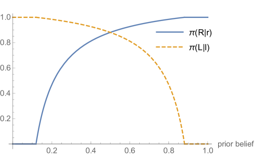
Figure 1: Solution to the problem (7) with different prior beliefs.

The principal prefers, ceteris paribus, to hire an agent who acquires more information and hence makes better choices – i.e., a more uncertain agent ($\mu$ close to $0.5$). However, if she believes that, e.g., state $r$ is ex ante more likely ($\mu_{p}>0.5$), then she, for all the same reasons as the agent, cares more about the agent choosing the optimal action in state $r$ than in state $l$. The latter leads her to prefer an agent who is not completely uncertain ($\mu\neq 0.5$), favoring those who agree with her in terms of which state is more likely ($\mu>0.5$). Balancing the two issues leads to the principal optimally hiring an agent who has a belief different from hers: $\mu\neq\mu_{p}$, yet who fundamentally agrees with her on the ex ante optimal action: $\mu\geq 0.5\iff\mu_{p}\geq 0.5$.

Figure 2 plots the principal’s expected utility from hiring an agent as a function of the agent’s belief $\mu$ when $\mu_{p}=0.7$. We can see the principal with a prior belief $\mu_{p}=0.7$ would prefer to hire an agent with a prior belief $\mu\approx 0.6$. Note that the graph is flat for very high and very low $\mu$, which corresponds to the agents who do not learn anything, and simply always choose the ex ante optimal action. Further, there exist agents with low $\mu\sim(0.15,0.25)$ who acquire non-trivial information, but hiring whom is worse for the principal than taking the ex ante optimal action (equivalent to hiring an agent with $\mu=1$). The latter demonstrates that if an agent is too biased, the information he acquires does not benefit the principal due to the bias in the agent’s actions resulting from his initial predisposition.

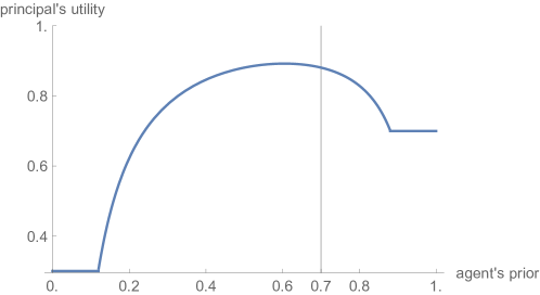
Figure 2: Expected utility of principal with prior belief $\mu_{p}=0.7$ as a function of the agent’s prior belief $\mu$.

The proposition 2 below formalizes this intuition and provides a closed-form solution for the optimal delegation strategy given the principal’s prior belief $\mu_{p}$. Figure 3 visualizes the optimal delegation strategy as a function of $\mu_{p}$.

Proposition 2.

If $\mathcal{M}=[0,1]$, then the principal’s optimal delegation strategy is given by

$$\mu^{*}=\frac{\sqrt{\mu_{p}}}{\sqrt{\mu_{p}}+\sqrt{1-\mu_{p}}}.$$ (13)

Therefore, if $\mu_{p}\in\left(\frac{1}{2},1\right)$, the principal optimally delegates to an agent with belief $\mu_{A}\in\left(\frac{1}{2},\mu_{p}\right)$.

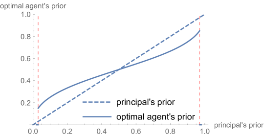
Figure 3: The optimal delegation strategy $\mu^{*}$ as a function of the principal’s prior belief $\mu_{p}$.

One thing to note about Proposition 2 is that the optimal delegation strategy (13) does not depend on the agent’s information cost factor, $\lambda$. While it is immediate that the higher is $\lambda$, the less information the agent with any given prior $\mu$ collects, Proposition 2 serves to show that the trade-off between the quantity of information and the bias in the decisions does not depend on the absolute quantity of information the agent acquires. Further, for a moderately high $\lambda$ (and/or a moderately extreme $\mu_{p}$), an agent with belief $\mu^{*}$ acquires no information, while an agent with belief $\mu=1/2$ would acquire some. In this case, it is nonetheless optimal for the principal to hire the $\mu^{*}$ agent (or, alternatively, simply choose the ex ante optimal action himself), since a learning agent would be too misaligned, and the benefits of information would be outweighed by the bias in the decisions.

Figure 4 demonstrates the difference in the action precisions between delegating to a perfectly aligned agent ($\mu=\mu_{p}$) and the optimally misaligned agent as given by (13). Optimal delegation leads to the agent consuming more information, lowers the probability of correctly matching the ex ante more likely (according to the principal’s belief $\mu_{p}$) state, $\pi(R|r)$, and increases $\pi(L|l)$, thereby bringing the two closer together. Overall, under the optimal delegation the less attractive ex-ante option is implemented relatively more frequently as compared to the case of the aligned delegation.

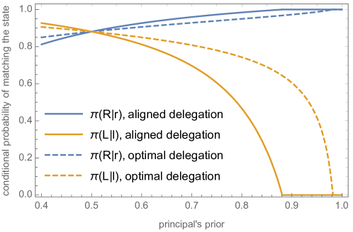
Figure 4: Action precisions under optimal delegation and delegating to the aligned agent.

An interesting connection can be made here to prospect theory (see Barberis, (2013) for a review). In particular, Tversky and Kahneman, (1992) suggest that in problems of choice under risk, individual decision-makers tend to succumb to cognitive biases such as overweighing small probabilities and underweighing large probabilities. They propose a probability weighting function that decision makers unconsciously use, which is reminiscent of our optimal delegation strategy (13), with $\mu_{p}$ being the objective probability and $\mu^{*}$ being the decision-maker’s perceived probability. Our result can thus be interpreted as one possible evolutionary explanation of the probability weighting functions. Namely, suppose that “Nature” (evolutionary pressure) is the principal and “Human” is the agent. They both have common utility function $u(a,\omega)$ representing the survival probability of the individual/population, but natural selection is indifferent towards the human’s cognitive costs $c(\phi,\mu)$ involved in the decision-making process. In this setting, natural selection would lead humans to develop probabilistic misperceptions according to (13), since these maximize the survival probability.

In the next section we generalize the binary model, assuming more available alternatives, while keeping the structure of the payoffs the same.

5 General Case

In this section we extend the analysis to a general problem of finding the best alternative, allowing for $N>2$ actions and states. We show that the principal’s optimal delegation strategy is qualitatively the same as in the binary case, i.e., it is optimal to hire a “more uncertain” agent, who considers more actions in search of the best one, relative to a fully aligned agent. Further, we characterize the whole set of decision rules that can be achieved by selecting the agent’s prior belief and show that it coincides with what can be achieved by selecting action-contingent subsidies for the agent.

We are now looking at the model with $\mathcal{A}\equiv\{a_{1},...,a_{N}\}$ and $\Omega\equiv\{\omega_{1},...,\omega_{N}\}$ for some $N$, and the preferences are given by $u(a_{i},\omega_{i})=1$ and $u(a_{i},\omega_{j})=0$ if $i\neq j$. Without loss of generality we assume that the principal’s belief $\mu_{p}$ is such that $\mu_{p}(\omega_{1})\geq\mu_{p}(\omega_{2})\geq\ldots\geq\mu_{p}(\omega_{N})$ (otherwise relabel states and actions as necessary). Same as before, the results from Section 3.5 apply, meaning that the agent’s problem is equivalent to choosing the action distribution $\pi:\Omega\to\varDelta(\mathcal{A})$ to maximize (4), and the principal selects an agent according to his prior $\mu\in\mathcal{M}$ to maximize (6). We do not restrict the choice of agents and let $\mathcal{M}=\varDelta(\Omega)$ (i.e., for any probability distribution $\mu\in\varDelta(\Omega)$, the principal can find and hire an agent with prior belief $\mu$).

5.1 Agent’s Problem

Proceeding by backward induction, we start by looking at the problem of an agent with some prior belief $\mu$. Invoking Theorem 1 from Matějka and McKay, (2015), as we did in the binary case, we can obtain the agent’s optimal decision rule:

$$\pi(a_{i}|\omega_{j})=\frac{\beta(a_{i})e^{\frac{u(a_{i},\omega_{j})}{\lambda}}}{\sum_{k=1}^{N}\beta(a_{k})e^{\frac{u(a_{k},\omega_{j})}{\lambda}}},$$ (14)

where $\beta(a_{i})$, defined in (5), is the unconditional choice probability according to the agent’s prior belief $\mu$. Corollary 2 from Matějka and McKay, (2015) shows that these probabilities solve the system of equations given by

$$\sum_{j=1}^{N}\mu(\omega_{j})\frac{e^{\frac{u(a_{i},\omega_{j})}{\lambda}}}{\sum_{k=1}^{N}\beta(a_{k})e^{\frac{u(a_{k},\omega_{j})}{\lambda}}}=1,$$ (15)

for every $i\in\{1,...,N\}$ such that $\beta(a_{i})>0$.

5.2 Principal’s Relaxed Problem

Note that (14) implies that a collection of the unconditional choice probabilities $\beta$ pins down the whole decision rule. Let us then consider a relaxed problem for the principal, in which instead of choosing agent’s prior $\mu$, she is free to select the unconditional choice probabilities $\beta\in\varDelta(\mathcal{A})$ directly:

$$\max_{\beta}\left\{\sum_{j=1}^{N}\mu_{p}(\omega_{j})\left(\sum_{i=1}^{N}\frac{\beta(a_{i})e^{\frac{u(a_{i},\omega_{j})}{\lambda}}}{\sum_{k=1}^{N}\beta(a_{k})e^{\frac{u(a_{k},\omega_{j})}{\lambda}}}u(a_{i},\omega_{j})\right)\right\}.$$ (16)

In the above, we used (14) to represent the conditional probabilities $\pi(a_{i}|\omega_{j})$ in (6) in terms of unconditional $\beta(a_{i})$. We show in Section 5.3 that the solution to this relaxed problem is implementable in the full problem.

Note that $\beta(a_{i})$ in the above represents the probability with which an agent expects to select action $a_{i}$. The principal’s expected probability of $a_{i}$ being selected, $\sum_{j=1}^{N}\mu_{p}(\omega_{j})\pi(a_{i}|\omega_{j})$, would generically be different, since her prior belief $\mu_{p}$ is different. Despite the potential confusion this enables, analyzing the principal’s problem through the prism of choosing $\beta$ is the most convenient approach due to the RI-logit structure of the solution to the agent’s problem.

Given the state-matching preferences $u(a_{j},\omega_{j})=1$, $u(a_{i},\omega_{j})=0$ if $i\neq j$, we can simplify (16) to

$$\max_{\beta}\left\{\sum_{j=1}^{N}\mu_{p}(\omega_{j})\frac{\beta(a_{j})e^{\frac{1}{\lambda}}}{1+\delta\beta(a_{j})}\right\},$$ (17)

where $\delta\equiv e^{\frac{1}{\lambda}}-1$. To characterize the solution to this relaxed problem, we need to introduce two new pieces of notation. For a given decision rule $\pi$, let $C(\beta)\equiv\left\{i\in\{1,...,N\}:\beta(a_{i})>0\right\}$ denote the consideration set, i.e., the set of actions that are chosen with strictly positive probabilities. Further, let $K(\beta)\equiv|C(\beta)|$ denote the power (number of actions in) this set. We can now state the solution to the principal’s problem as follows.

Lemma 1.

The solution to the principal’s relaxed problem (17) is given by

$$\beta^{*}(a_{i})=\max\left\{0,\frac{1}{\delta}\left(\frac{(K(\beta^{*})+\delta)\sqrt{\mu_{p}(\omega_{i})}}{\sum\limits_{j\in C(\beta^{*})}\sqrt{\mu_{p}(\omega_{j})}}-1\right)\right\},$$

where $\delta\equiv e^{\frac{1}{\lambda}}-1$.

Lemma 1 describes the solution in terms of the action choice probabilities, which do not necessarily give the reader a good idea of its features and the intuition behind this solution. We explore these in more detail in Section 5.4. Before that, however, we need to ensure that this solution is attainable in the principal’s full problem, which is done in the following section.

5.3 Principal’s Full Problem

The question this section explores is: can the principal generate choice probabilities $\beta^{*}$ by appropriately choosing the agent’s prior belief $\mu$? In the binary case, the answer was trivially “yes”: due to continuity of the agent’s strategy, by varying the agent’s belief $\mu(r)$ between $0$ and $1$, the principal could induce any unconditional probability $\beta(R)$. In the multidimensional case, this is not immediate. However, the following theorem shows that the result still holds with $N$ actions and states under state-matching preferences.

Theorem 1.

In the principal’s full problem (6), any vector $\beta\in\varDelta(\mathcal{A})$ of unconditional choice probabilities is implementable: there exists a prior belief $\mu\in\varDelta(\Omega)$ such that $\beta(a_{i})=\sum_{j=1}^{N}\mu(\omega_{j})\pi^{*}_{\mu}(a_{i}|\omega_{j})$, where $\pi^{*}_{\mu}$ solves the agent’s problem (4) given $\mu$.

The theorem states that if $\mathcal{M}=\varDelta(\Omega)$, then the principal can generate any vector of unconditional action probabilities. Note that this does not imply that she is able to select any decision rule $\pi(a_{i}|\omega_{j})$ – if this were the case, under the state-matching preferences she would simply choose to have $\pi(a_{i}|\omega_{i})=1$ for all $i$. However, Theorem 1 does imply that the choice probabilities described in Lemma 1 – those that solve the principal’s relaxed problem, – are implementable and thus also solve her full problem.

The result does, however, rely on the state-matching preferences: we show in Section 6.1 that it does not hold for arbitrary payoffs.

5.4 Properties of the Optimal Delegation Strategy

While Lemma 1 presents the solution of the principal’s problem in terms of the unconditional choice probabilities, this representation is not the most visual. We now demonstrate some implications of this solution in terms of other variables. Namely, Proposition 3 extends Proposition 2 and shows how the chosen agent’s prior belief relates to that of the principal. Proposition 4 then compares actions taken under optimal delegation vs aligned delegation.

We begin by looking at the optimal agent choice in terms of the agent’s belief $\mu^{*}$.

Proposition 3.

The principal’s equilibrium delegation strategy $\mu^{*}$ is such that for all $i,j\in\{1,...,N\}$:

$$\frac{\mu^{*}(\omega_{i})}{\mu^{*}(\omega_{j})}=\frac{\sqrt{\mu_{p}(\omega_{i})}}{\sqrt{\mu_{p}(\omega_{j})}}.$$

In particular, $\mu^{*}(\omega_{1})\geq...\geq\mu^{*}(\omega_{N})$. Further, $\mu^{*}(\omega_{1})\leq\mu_{p}(\omega_{1})$ and $\mu^{*}(\omega_{N})\geq\mu_{p}(\omega_{N})$, with equalities if and only if $\mu_{p}(\omega_{1})=...=\mu_{p}(\omega_{j})$.

The intuition behind the proposition above is the same as behind Proposition 2: the optimally chosen agent is more uncertain than the principal between any given pair of states. To see this, note that if $\mu_{p}(\omega_{i})>\mu_{p}(\omega_{j})$ then $1<\frac{\mu^{*}(\omega_{i})}{\mu^{*}(\omega_{j})}<\frac{\mu_{p}(\omega_{i})}{\mu_{p}(\omega_{j})}$ – i.e., the agent believes state $\omega_{i}$ is ex ante more likely than $\omega_{j}$, as the principal does, but he assigns relatively less weight to $\omega_{i}$. This applies to any pair of states, so the implication is that the optimal agent must assign a lower ex ante probability to $\omega_{1}$, the most likely state according to the principal, than she does, and vice versa for $\omega_{N}$. Note further that the result in Proposition 3 is again independent of $\lambda$, implying that the optimal delegation strategy is determined by the relative trade-off between the quantity of information acquired and the bias introduced in actions by the misalignment in beliefs, but the absolute quantity of information acquired is irrelevant. In particular, hiring an agent with $\mu^{*}$ is optimal even when he acquires no information, and another agent $\mu$ is available, who would be willing invest effort in learning $\omega$ (since such a $\mu$-agent would be too biased relative to the principal).

We now switch to comparing the choices made under optimal delegation to those that would arise under aligned delegation – i.e., if the principal selected an agent with $\mu=\mu_{p}$. Let $\bar{\beta}$ denote the choice probabilities that would be generated under aligned delegation. Caplin et al., (2019) show that these probabilities $\bar{\beta}$, as a function of the agent’s prior $\mu$, are given by (see their Theorem 1)

$$\bar{\beta}(a_{i})=\max\left\{0,\frac{1}{\delta}\left(\frac{(K(\bar{\beta})+\delta){\mu(\omega_{i})}}{\sum\limits_{j\in C(\bar{\beta})}{\mu(\omega_{j})}}-1\right)\right\}.$$ (18)

Since $\mu_{p}(\omega_{1})>...>\mu_{p}(\omega_{N})$, the consideration set in the aligned problem is then simply $C(\bar{\beta})=\{1,...,\bar{K}\}$, and its size $\bar{K}\equiv K(\bar{\beta})$ is the unique solution of

$$\mu_{p}(\omega_{\bar{K}})>\frac{1}{\bar{K}+\delta}\sum_{j=1}^{\bar{K}}\mu_{p}(\omega_{j})\geq\mu_{p}(\omega_{\bar{K}+1}).$$ (19)

In turn, we can see from Lemma 1 that under optimal delegation, size $K^{*}=K(\beta^{*})$ of the consideration set under optimal choice is

$$\sqrt{\mu_{p}(\omega_{K^{*}})}>\frac{1}{K^{*}+\delta}\sum_{j=1}^{K^{*}}\sqrt{\mu_{p}(\omega_{j})}\geq\sqrt{\mu_{p}(\omega_{K^{*}+1})}.$$ (20)

These two conditions allow us to compare $K^{*}$ and $\bar{K}$ directly, which is done by the following proposition.

Proposition 4.

Optimal delegation weakly expands the consideration set relative to aligned delegation:

$$K(\beta^{*})\geq K(\bar{\beta}).$$

In other words, delegating to an optimally misaligned agent leads to a wider variety of actions played in equilibrium. This is a direct consequence of delegation to a more uncertain agent – since he is less sure than the principal of what the optimal action is ex ante, he considers more actions as worth investigating. Every action has some positive probability of actually being optimal, thus a more uncertain agent plays a wider range of different actions ex post. We could already see this effect at play in the binary case, where if $\mu_{p}$ is extreme, then an aligned agent takes the ex ante optimal action without acquiring any additional information, whereas the optimally chosen agent could investigate both actions.

6 Misaligned Beliefs Versus Other Instruments

The preceding analysis above explored the problem of selecting an agent according to their prior belief. It gave grounds for using the misaligned beliefs as an instrument in delegation, yet it still worth studying how this instrument compares to the other instruments, such as contracting or restricting the delegation set. In this section, we draw this comparison. We keep the overall structure of the problem the same as in Section 5, but now consider three separate versions, in which the principal has different tools at her disposal, and compare outcomes to those in the baseline problem of choosing agent’s beliefs.

6.1 Contracting on Actions/Misaligned Preferences

The most basic delegation tool is contracting: if the principal could offer the agent a contract that specifies contingent payments, this would be the most direct way to provide incentives. We can think of two main options here: contracting on outcomes (where “outcome” is understood in the sense of “was the agent’s action correct?”) and contracting on actions. The former requires that both outcomes are contractible (i.e., observable and verifiable), the latter imposes such requirement on actions. Both options require that the principal has the freedom to design the payments, which is a strong assumption in itself.

We begin by exploring the contracting on actions in our framework, in which the principal must design a payment schedule $\{\tau(a_{i})\}$ to be paid to the agent. We assume that all agents and the principal have a common prior belief $\mu_{p}$, all players’ preferences are quasilinear in payments, and the principal’s marginal utility of money is $\rho$, and the agent’s marginal utility of money is $1$. For some results, we additionally impose the limited liability assumption ($\tau(a_{i})\geq 0$ for all $i$).

Note that instead of contracting, we can interpret this setup as a problem of selecting an agent with misaligned preferences by setting $\rho=0$. Collection $\{\tau(a_{i})\}$ then represents an agent’s “biases”, i.e., inherent preferences towards certain actions on top of the “unbiased” utility $u(a,\omega)$. Such a problem of selecting an agent with optimally misaligned preferences is a natural counterpart to our baseline problem of selecting an agent with optimally misaligned beliefs.

The agent’s problem (again using the equivalence presented in 3.5) is then given by

$$\max_{\pi}\Bigg{\{}\sum_{j=1}^{N}\mu_{p}(\omega_{j})\sum_{i=1}^{N}\pi(a_{i}|\omega_{j})\big{(}u(a_{i},\omega_{j})+\tau(a_{i})\big{)}-c(\phi,\mu_{p})\Bigg{\}},$$ (21)

given $\tau$, and the principal’s contracting problem is

$$\max_{\tau} \left\{\sum_{j=1}^{N}\mu_{p}(\omega_{j})\sum_{i=1}^{N}\pi(a_{i}|\omega_{j})\big{(}u(a_{i},\omega_{j})-\rho\tau(a_{i})\big{)}\right\},$$ (22)

subject to $\pi$ solving (21) given $\tau$.

Instead of providing a closed-form solution to this problem, we appeal to Theorem 1 to argue that regardless of $\rho$, the principal cannot obtain higher expected utility than in the baseline problem of choosing an agent with a misaligned belief $\mu$. In particular, Theorem 1 implies that any unconditional choice probabilities $\beta\in\varDelta(\mathcal{A})$ generated by an agent, who is incentivized by payments or misaligned preferences, can also be obtained by selecting an agent with appropriately misaligned beliefs. Moreover, if we relax limited liability and allow negative payments, then by using results of Matveenko and Mikhalishchev, (2021) we can also show the converse – that any choice rule achievable with misaligned beliefs can be replicated with payments $\tau$ (or by setting the quotas – i.e., imposing specific unconditional choice probabilities for different action). These results are formalized in the following proposition.

Proposition 5.

The principal’s problem of contracting on actions (22) is equivalent to her full (delegation) problem (6):

1. For any vector $\tau:\mathcal{A}\to\mathbb{R}$ of payments/biases and a corresponding $\beta:\Omega\to\varDelta(\mathcal{A})$ that solves (21) given $\tau$, there exists a prior belief $\mu\in\varDelta(\Omega)$ such that $\beta$ also solves (4) given $\mu$.

2. For any $\mu\in\varDelta(\Omega)$ and the corresponding $\beta:\Omega\to\varDelta(\mathcal{A})$ that solves (4) given $\mu$, there exist payments $\tau:\mathcal{A}\to\mathbb{R}$ such that $\beta$ also solves (21) given $\tau$.

The proposition above directly implies that neither of the two instruments (contracting on actions or searching for an agent with stronger/weaker preferences for specific actions) can yield better results than hiring an agent with an optimally misaligned belief. If limited liability is in place ($\tau(a_{i})\geq 0$ for all $i$), then contracting on actions is strictly worse, since it cannot yield a better decision rule, but requires payments from the principal – payments which are avoidable if she instead hires an agent who is intrinsically motivated by his beliefs over states or preferences towards specific actions.

Further, Theorem 1 and the results of Matveenko and Mikhalishchev, (2021) also imply that the space of solutions to either problem covers the whole universe of RI-logit choice rules given fixed preferences between states. This implies that no combination of misaligned beliefs, misaligned preferences, and payments for actions can perform better than any individual instrument. Moreover, it also implies that suboptimal misalignment along any dimension can be amended using other instruments. I.e., if a given agent holds a non-optimal prior belief (that does not coincide with the principal’s either), the optimal behavior might be induced via action-contingent transfers. Conversely, if all agents are biased towards certain actions, this misalignment can be compensated for by selecting an agent with the right prior belief. The following proposition presents one example of such equivalence, in the context of a model with $N=2$.

Proposition 6.

Consider the binary setting of Section 4. Consider the principal’s problem of contracting on actions (22), where $\rho=0$ and the agent holds prior belief $\mu\neq\mu_{p}$. Then:

1. for any $\mu$, there exist payments/biases $\{\tau^{*}(L),\tau^{*}(R)\}$ that implement the optimal conditional choice probabilities from Section 4;

2. these payments/biases are such that

   $$\tau^{*}(R)\geq\tau^{*}(L)\iff\mu\leq\mu^{*}=\frac{\sqrt{\mu_{p}}}{\sqrt{\mu_{p}}+\sqrt{1-\mu_{p}}}.$$

It is easy to see the intuition behind the proposition: if the agent’s prior belief $\mu$ assigns lower probability to state $\omega=r$ compared to the principal-optimal prior $\mu^{*}$ given in Proposition 2, such an agent is ex ante too biased towards action $L$ for the principal’s taste, even though he potentially acquires more information than an agent with belief $\mu^{*}$. Therefore, the principal can nudge the agent towards action $R$ by offering higher payment if he selects $R$ (or find an agent, whose preference bias towards $R$ offsets his belief bias towards state $l$).

6.2 Contracting on Outcomes

We now turn to contracting on outcomes. The outcome in our model is effectively binary: whether a correct action was chosen ($a=a_{j}$ when $\omega=\omega_{j}$) or not. We thus let the principal select payments $\bar{\tau},\underline{\tau}$ that the agent receives, so that $\tau(a_{i},\omega_{i})=\bar{\tau}$ and $\tau(a_{i},\omega_{j})=\underline{\tau}$ if $i\neq j$. We again assume limited liability ($\bar{\tau},\underline{\tau}\geq 0$), preferences that are quasilinear in payments for all agents, and let the agent’s marginal utility of money to be $1$, and the principal’s marginal utility of money to be $\rho$.

The agent’s problem is then choosing $\pi:\Omega\to\varDelta(\mathcal{A})$ that solves

$$\max_{\pi}\Bigg{\{}\sum_{j=1}^{N}\mu(\omega_{j})\sum_{i=1}^{N}\pi(a_{i}|\omega_{j})\big{(}u(a_{i},\omega_{j})+\tau(a_{i},\omega_{j})\big{)}-c(\phi,\mu)\Bigg{\}},$$ (23)

and the principal’s contracting problem is

$$\max_{\bar{\tau},\underline{\tau}} \left\{\sum_{j=1}^{N}\mu_{p}(\omega_{j})\sum_{i=1}^{N}\pi(a_{i}|\omega_{j})\big{(}u(a_{i},\omega_{j})-\rho\tau(a_{i},\omega_{j})\big{)}\right\},$$ (24)

s.t. $$\tau(a_{i},\omega_{i})=\bar{\tau}\text{ for all }i,$$

$$\tau(a_{i},\omega_{j})=\underline{\tau}\text{ for all }i,j\neq i,$$

and subject to $\beta$ corresponding to a solution of (23) given $\bar{\tau},\underline{\tau}$.

It is trivially optimal for the principal to set $\underline{\tau}=0$, since her objective is to provide incentives for the agent to match the state. Then, however, the agent’s (ex post) payoff net of information cost becomes $u(a_{i},\omega_{j})+\tau(a_{i},\omega_{j})=(1+\bar{\tau})u(a_{i},\omega_{j})$, and the principal’s payoff is $u(a_{i},\omega_{j})-\tau(a_{i},\omega_{j})=(1-\rho\bar{\tau})u(a_{i},\omega_{j})$. In other words, by increasing the incentive payment $\bar{\tau}$, the principal effectively lowers the relative cost of information for the agent, at the cost of decreasing her own payoff. It then appears like an instrument that could be universally useful for the principal – even when she chooses an agent with the optimal prior belief, she could still benefit from reducing the agent’s information cost, which would result in him acquiring more information. The following proposition shows, however, that this is not the case: while contracting on outcomes may be a useful instrument, it cannot improve on delegating to the optimally biased agent when payments are costly to the principal.

Proposition 7.

Consider the principal’s contracting problem (24) in the binary setting of Section 4 and suppose $\rho=1$ and $\mu_{p}>1/2$. Then there exist $\bar{\mu}_{1},\bar{\mu}_{2}$: $\bar{\mu}_{1}<\mu^{*}<\mu_{p}<\bar{\mu}_{2}$ (where $\mu^{*}$ is as in Proposition 2), such that if either $\frac{1}{1+e^{\frac{1}{\lambda}}}\leq\mu\leq\bar{\mu}_{1}$, or $\bar{\mu}_{2}\leq\mu\leq\frac{e^{\frac{1}{\lambda}}}{1+e^{\frac{1}{\lambda}}}$, then $\bar{\tau}>0$ solves (24).

The proposition states that the principal uses the incentive payments, $\bar{\tau}>0$, when there is an intermediate degree of misalignment in opinions with the agent. If the agent has a very extreme prior belief and acquires no information on his own, it may be too costly for the principal to incentivize such an agent to acquire any information. The requirements that $\frac{1}{1+e^{\frac{1}{\lambda}}}\leq\mu\leq\frac{e^{\frac{1}{\lambda}}}{1+e^{\frac{1}{\lambda}}}$ ensure that the agent acquires information voluntarily so that this problem does not arise. On the other hand, if there is too little misalignment ($\bar{\mu}_{1}<\mu<\bar{\mu}_{2}$), then the agent’s information acquisition choice is already in line with the principal’s wishes, and any further payments would not have a significant enough effect on the agent’s incentives to justify the cost they incur on the principal.

6.3 Restricting the Delegation Set

Another instrument commonly explored in the delegation literature is restricting the delegation set – i.e., the set of actions that the agent may take (see, e.g., Holmstrom, (1980)). In particular, in the context of “delegated expertise” problems, Szalay, (2005) and Ball and Gao, (2021) show that it may be optimal to rule out an ex ante optimal action in order to force the agent to exert effort and learn which of the ex post optimal (but ex ante risky) actions is best. Lipnowski et al., (2020) show a similar result in a Bayesian Persuasion setting, where the receiver is rationally inattentive to the sender’s message.

In our setting, however, there are no “safe” actions that the principal could rule out, as Propostion 4 suggests. Assuming that the principal and the agent hold the same prior belief $\mu_{p}$, and $\mu_{p}(\omega_{1})>...>\mu_{p}(\omega_{N})$, action $a_{1}$ is the “safest” in the sense of being the most likely ex ante to be optimal. Yet, it would be trivially suboptimal for the principal to ban $a_{1}$ – since, indeed, this is the action that is ex ante most likely to be ex post optimal! In other words, while excluding $a_{1}$ from the delegation set would lead the agent to acquire more information, it would also lead to larger ex post losses due to the agent being unable to select action $a_{1}$ in cases when it is optimal to do so. So while the general idea of the principal being willing to nudge the agent to acquire more information/information about ex ante suboptimal actions holds true in our setting, restricting the delegation set is not an instrument that lends any value to the principal.

Proposition 8 below summarizes this logic. Consider the agent’s problem as given by

$$\max_{\pi}\Bigg{\{}\sum_{j=1}^{N}\mu_{p}(\omega_{j})\sum_{i=1}^{N}\pi(a_{i}|\omega_{j})u(a_{i},\omega_{j})-c(\phi,\mu_{p})\Bigg{\}},$$ (25)

given $A^{*}\subseteq\mathcal{A}$ (and the maximization is w.r.t. a mapping $\pi:\Omega\to\varDelta(A^{*})$), and the principal’s restriction problem

$$\max_{A^{*}} \left\{\sum_{j=1}^{N}\mu_{p}(\omega_{j})\sum_{i=1}^{N}\pi(a_{i}|\omega_{j})u(a_{i},\omega_{j})\right\},$$ (26)

subject to $\pi:\Omega\to\varDelta(A^{*})$ solving (25) given $A^{*}$. Then we can state the result as follows.

Proposition 8.

The unrestricted delegation set $A^{*}=\mathcal{A}$ is always a solution to the principal’s restriction problem (26).

7 Extensions

7.1 Alternative Preference Specifications

The analysis in Sections 5 and 6.1 is heavily reliant on state-matching preferences that we assume are shared by both the principal and the agent(s). It is reasonable to ask whether our conclusions hold under other preference specifications. Since the utility function $u(a,\omega)$ is shared by both the principal and the agent, it is reasonable to generalize one at a time.

We begin by generalizing the principal’s utility function $u_{p}(a,\omega)$ while maintaining the agent’s intrinsic preference for matching the state: $u_{A}(a_{i},\omega_{i})=1$, $u_{A}(a_{i},\omega_{j})=0$ if $i\neq j$. Naturally, the specific functional forms of the optimal delegation strategies (such as those presented in Propositions 2 and 3, and Lemma 1) depend on the specific form of the principal’s utility function. However, Theorem 1 only depends on the agent’s utility function, meaning that Proposition 5 still holds: any outcome that can be achieved by contracting on actions or hiring an agent with the misaligned intrinsic preferences, can also be achieved by hiring an agent with misaligned beliefs (and vice versa). Meaning that regardless of the principal’s objective function, hiring an agent with state-matching preferences and a suitable belief is as good as hiring an agent with aligned prior belief, state-matching preferences, and either some additional preference over actions, or action-contingent payments on top of that.

The above does, however, hinge on the agent having state-matching preferences as a baseline. Once we allow arbitrary preferences for the agent – even if they align with the principal’s preferences net of the information cost – the equivalence stated in Proposition 5 breaks down. In such a general case, finding an agent with optimally misaligned preferences may yield strictly better results for the principal than hiring an agent with an optimally misaligned belief, and hence contracting on actions may, in principle, yield better results too. An example (for misaligned preferences) is presented in the proof of the following proposition.

Proposition 9.

There exists a utility function $u(a_{i},\omega_{j})$ with $u(a_{i},\omega_{i})=\max\limits_{k}\{u(a_{k},\omega_{i})\}$ such that the solution of the principal’s relaxed problem (17) can not be attained as a solution of the full problem (6).

The optimal choice rule is never in the relative interior, since mixing between two options dominates using mixing from three. However, according to Proposition 3 and Lemma 1 from Matveenko and Mikhalishchev, (2021), the principal may implement the optimal solution via action-contingent payments/biased preferences.

7.2 Communication

In this section we consider the importance of decision rights in our model with misaligned beliefs. In particular, we juxtapose the delegation scheme explored so far, under which the agent has the power to make the final decision, to communication, where an agent must instead communicate his findings to the principal, who then chooses the action. A large literature in organizational economics is devoted to comparing delegation and communication in various settings (see Dessein, (2002); Alonso et al., (2008), and Rantakari, (2008) for some examples). We show that in our setting, communication performs as well as delegation – i.e., the principal will always find it optimal to follow the agent’s recommendation. This is, perhaps, unsuprising, since Holmstrom, (1980) showed that communication is equivalent to restricting the agent’s action set, and this latter problem was shown in Section 6.3 to be an irrelevant instrument in our setting, as long as the principal can select an agent with the prior belief she prefers.

Although the principal and an agent have the same preferences, it is generally unclear whether it is optimal for the principal to follow a recommendation of an agent due to the misalignment in their beliefs. Namely, since the principal and the agent start from different prior beliefs, the same is true for posteriors: if the principal could observe the information that the agent obtained, her posterior belief would be different from that of the agent. This implies that ex post, the principal could prefer an action different from the agent’s choice, and could benefit ex post from overruling the agent’s decision if she had the power to do so. However, this would mean that the agent’s incentives to acquire information are different from the baseline model, and could lead to the agent acquiring either more or less information than in the baseline, with the principal having some influence over the agent’s learning strategy via her final decision rule. We show below that in the end, none of these effects come into play, and there exists a communication equilibrium that replicates the delegation equilibrium.

The setup follows the baseline model from Section 3, with the exception that the final stage (“agent selecting action $a\in\mathcal{A}$”) is replaced by two. First, after observing signal $s\in\mathcal{S}$ generated by his signal structure $\phi$, the agent selects a recommendation (message) $\tilde{a}\in\mathcal{A}$ to the principal. After that, the principal observes the recommendation $\tilde{a}$, uses it to update her belief $\mu_{p}(\omega|\tilde{a})$ about the state of the world, and then selects an action $a\in\mathcal{A}$ that determines the both parties’ payoffs. The equilibrium of the communication game is then defined as follows.

Definition (Communication Equilibrium).

An equilibrium of the cheap talk game is characterized by $(\mu^{*},\{\phi^{*}_{\mu},\tilde{\sigma}^{*}_{\mu}\}_{\mu\in\mathcal{M}},\sigma^{*},\mu_{p})$, which consists of the following:

1. the principal’s posterior beliefs $\mu_{p}:\mathcal{A}\to\varDelta(\Omega)$ that are consistent with $(\phi^{*}_{\mu},\sigma^{*}_{\mu})$ (i.e., satisfy Bayes’ rule on the equilibrium path);

2. the principal’s decision rule $\sigma^{*}:\mathcal{A}\to\mathcal{A}$, which solves the following for every $\tilde{a}\in\mathcal{A}$, given the posterior $\mu_{p}$:

   $$\max_{\sigma(\tilde{a})}\left\{\sum_{\omega\in\Omega}\mu_{p}(\omega|\tilde{a})u(\sigma(\tilde{a})|\omega)\right\};$$

3. a collection of the agents’ information acquisition strategies $\phi^{*}_{\mu}:\Omega\to\varDelta(\mathcal{S})$ and communication strategies $\tilde{\sigma}^{*}_{\mu}:\mathcal{S}\to\mathcal{A}$ that solve the following given $\sigma$ for every $\mu\in\mathcal{M}$:

   $$\max_{\phi,\tilde{\sigma}}\left\{\sum_{\omega\in\Omega}\mu(\omega)\sum_{s\in\mathcal{S}}\phi(s|\omega)u(\sigma(\tilde{\sigma}(s)),\omega)-c(\phi,\mu)\right\};$$

4. the principal’s choice $\mu^{*}\in\mathcal{M}$ of the agent to whom the task is delegated, which solves the following given $(\phi^{*}_{\mu},\sigma^{*}_{\mu})$, $\sigma^{*}$, and $\mu_{p}$:

   $$\max_{\mu} \left\{\sum_{\omega\in\Omega}\mu_{p}(\omega)\sum_{s\in\mathcal{S}}\phi(s|\omega)u(\sigma(\tilde{\sigma}(s)),\omega)\right\}.$$

We can then state the result as follows.

Proposition 10.

There exists a communication equilibrium that is outcome-equivalent to the equilibrium of the original game, in the sense that $(\mu^{*},\phi^{*}_{\mu^{*}},\tilde{\sigma}^{*}_{\mu^{*}})$ are the same in both equilibria, and $\sigma^{*}$ is an identity mapping.

This result, however, is subject to a few caveats. First, cheap talk models are plagued by equilibrium multiplicity: for any informative equilibrium, there exist equilibria with less informative communication, up to completely uninformative (babbling) equilibria. In our setting this means that in addition to the equilibrium outlined in Proposition 10 above, there also exists a babbling equilibrium, in which the agent acquires no information and makes a random recommendation, and the principal always ignores it and selects the ex ante optimal action. There would also likely exist multiple equilibria of intermediate informativeness – e.g., equilibria with a limited vocabulary, where only some actions $\tilde{\mathcal{A}}\subset\mathcal{A}$ are recommended on equilibrium path. In practice, this means that under communication, there is a risk of miscoordination on uninformative equilibria, whereas under delegation the equilibrium is unique. The same force may also work the other way, and there may be equilibria that are preferred by the principal to the delegation equilibrium, that can only be sustained under cheap talk (see Argenziano et al., (2016) for an example of how such equilibria may arise). However, the question of whether such equilibria exist is beyond the scope of this paper.

The second caveat lies in the fact that Proposition 10 relies on the state-matching preferences. In our setting (with the exception of Section 7.1), any action is either “right” or “wrong”, without any degrees of correctness. The misalignment of beliefs across the principal and the agent is thus small enough to not warrant the principal overriding the agent’s suggested action. In contrast, in a uniform-quadratic framework, both states and actions lie in a continuum, and the principal’s loss is proportional to the distance between the realized state and the chosen action. In such a setting, any misalignment (be it in preferences or beliefs) between the principal and the agent would lead to the principal being willing to override the agent’s recommendation, leading to the delegation equilibrium being no longer directly sustainable under communication.

8 Conclusion

We show that hiring an agent with beliefs that are misaligned with those of the principal can be beneficial for the principal, contrary to popular belief. In particular, if the agent needs to acquire information to make a decision, delegation to an agent who is ex ante more uncertain about what the best action is but shares some of the principal’s predispositions is optimal for her. This is mainly due to a more uncertain agent being willing to acquire more information about the state, which enables more efficient actions being taken. We show that exploiting belief misalignment can be a valid instrument that the principal can use in delegation, which in some settings is on par with or better than state-contingent transfers or restriction of the action set from which the agent can choose.

In the analysis, we use the workhorse rational inattention model for discrete choice, the Shannon model. It allows us to provide a richer demonstration of the consequences of delegation to a biased agent by allowing the agent to acquire information flexibly, which introduces additional bias into the decisions of an agent with misaligned beliefs. We show that misaligned delegation is optimal despite the bias introduced by this flexibility. Hence, while the exact trade-offs do, obviously, depend on the particular cost function specification, the main takeaways would persist regardless of the form of the costs of information.

Our analysis focuses on misalignment and away from contracting. A potentially fruitful avenue for further research would be to consider more carefully the contracting problem in a setting where the principal and the agent have misaligned beliefs and/or preferences, and to investigate how contracting can build upon the inherent benefits of misalignment.

Further, due to the added complexity of rational inattention models, we confine our exploration to a discrete state-matching model, which strays away from the continuous models more commonly used in delegation problems. In a model with continuous actions, the scope for an agent to manifest his bias is much larger, hence the trade-off between the agent’s information acquisition and biased decision-making would again be different. Exploration of the effects of misalignment in a continuous model of delegated expertise could be an interesting direction for further research as well.

Yet another assumption that may feel excessively strong in our analysis is the common knowledge of all agents’ and the principal’s prior beliefs. It may be more reasonable to assume that agents are strategic in presenting their viewpoints to the principal, as well as making inferences from the fact that they were chosen for the job. Such signaling concerns could yield an economically meaningful effect, yet we abstract from them completely in our paper. A more careful investigation is in order.

Appendix A Main Proofs

A.1 Proof of Proposition 2

Throughout this proof, we will refer to the delegation rule under consideration,

$$\mu^{*}=\frac{\sqrt{\mu_{p}}}{\sqrt{\mu_{p}}+\sqrt{1-\mu_{p}}},$$

as the candidate rule. It is straightforward that under the candidate rule, if $\mu_{p}>\frac{1}{2}$ then $\mu^{*}\in\left(\frac{1}{2},\mu_{p}\right)$, since

$$\frac{\mu^{*}}{1-\mu^{*}}=\frac{\sqrt{\mu_{p}}}{\sqrt{1-\mu_{p}}}<\frac{\mu_{p}}{1-\mu_{p}}$$

when $\mu_{p}>\frac{1}{2}$, so $\mu^{*}<\mu_{p}$, and also $\sqrt{\mu_{p}}>\sqrt{1-\mu_{p}}$ in that case, so $\mu^{*}>\frac{1}{2}$. It thus remains to show that the candidate rule is indeed optimal for the principal. While a shorter proof exists that invokes Lemma 1 that derives an optimal strategy for the case of $N$ states and actions, we choose to present a more direct, albeit a somewhat longer, proof.

Plugging the solution of the agent’s problem (11) (assuming this solution is interior for now) into the principal’s problem (12), we get that the principal’s payoff looks as follows:

$$\mu_{p}\pi(R|r)+(1-\mu_{p})\pi(L|l) =\mu_{p}\frac{\left(\mu e^{\frac{1}{\lambda}}-(1-\mu)\right)e^{\frac{1}{\lambda}}}{\left(e^{\frac{2}{\lambda}}-1\right)\mu}+(1-\mu_{p})\frac{\left((1-\mu)e^{\frac{1}{\lambda}}-\mu\right)e^{\frac{1}{\lambda}}}{\left(e^{\frac{2}{\lambda}}-1\right)(1-\mu)}$$

$$=\frac{e^{\frac{1}{\lambda}}}{e^{\frac{2}{\lambda}}-1}\left[\mu_{p}\left(e^{\frac{1}{\lambda}}-\frac{1-\mu}{\mu}\right)+(1-\mu_{p})\left(e^{\frac{1}{\lambda}}-\frac{\mu}{1-\mu}\right)\right]$$

$$\propto e^{\frac{1}{\lambda}}-\mu_{p}\frac{1-\mu}{\mu}-(1-\mu_{p})\frac{\mu}{1-\mu}.$$

The FOC for the principal’s maximization problem above w.r.t. $\mu$ is

$$\frac{\mu_{p}}{\mu^{2}}-\frac{1-\mu_{p}}{(1-\mu_{p})^{2}}=0$$

$$\iff \frac{\mu}{1-\mu}=\frac{\sqrt{\mu_{p}}}{\sqrt{1-\mu_{p}}}.$$ (27)

It is trivial to verify that the second-order condition holds as well, hence as long as (27) yields an interior solution (i.e., the probabilities in (11) are in $[0,1]$), the candidate solution is indeed optimal among all such interior solutions.

We now check for which $\mu$ the solution (11) is interior. Using the expressions (11), one can easily verify that $\pi(R|r)\geq 0\iff\frac{\mu}{1-\mu}\geq e^{-\frac{1}{\lambda}}$ and $\pi(R|r)\leq 1\iff\frac{\mu}{1-\mu}\leq e^{\frac{1}{\lambda}}$, and the conditions $\pi(L|l)\in[0,1]$ yield the same two interiority conditions. This implies that if $\frac{\mu}{1-\mu}\in\left[e^{-\frac{1}{\lambda}},e^{\frac{1}{\lambda}}\right]$, then the agent acquires some information and selects both actions with positive probabilities, and otherwise $(\pi(R|r),\pi(L|l))\in\{(1,0),(0,1)\}$, meaning that the agent simply chooses the ex ante optimal action for sure without acquiring any information about the state.

The candidate rule then suggests that the principal delegates to a learning agent iff $\frac{\mu_{p}}{1-\mu_{p}}\in\left[e^{-\frac{2}{\lambda}},e^{\frac{2}{\lambda}}\right]$, and otherwise delegates to an agent who plays the ex ante optimal action. We have shown that the candidate rule selects the optimal among the learning agents; it is left to verify that such a choice rule between learning and non-learning agents is optimal for the principal.

Consider $\mu_{p}\geq\frac{1}{2}$; then among the non-learning agents the principal would obviously choose the one who plays $a=R$ (rather than $a=L$), and such a choice yields the principal expected payoff $\mu_{p}\cdot 1+(1-\mu_{p})\cdot 0=\mu_{p}$. Optimal delegation to a learning agent yields (by plugging the candidate rule into the principal’s payoff obtained above)

$$\frac{e^{\frac{1}{\lambda}}}{e^{\frac{2}{\lambda}}-1}\left[e^{\frac{1}{\lambda}}-\mu_{p}\frac{1-\mu^{*}}{\mu^{*}}-(1-\mu_{p})\frac{\mu^{*}}{1-\mu^{*}}\right]= \frac{e^{\frac{1}{\lambda}}}{e^{\frac{2}{\lambda}}-1}\left[e^{\frac{1}{\lambda}}-2\sqrt{\mu_{p}(1-\mu_{p})}\right].$$ (28)

Taking the difference between (28) and $\mu_{p}$, the payoff from delegating to a non-learning agent, lets us find belief $\mu_{p}$ of a principal who would be indifferent between the two:

$$\frac{e^{\frac{1}{\lambda}}}{e^{\frac{2}{\lambda}}-1}\left[e^{\frac{1}{\lambda}}-2\sqrt{\mu_{p}(1-\mu_{p})}\right]-\mu_{p}=0$$

$$\iff e^{\frac{2}{\lambda}}-2e^{\frac{1}{\lambda}}\sqrt{\mu_{p}(1-\mu_{p})}=\mu_{p}e^{\frac{2}{\lambda}}-\mu_{p}$$

$$\iff \left(e^{\frac{1}{\lambda}}\sqrt{1-\mu_{p}}-\sqrt{\mu_{p}}\right)^{2}=0$$

$$\iff \frac{\sqrt{\mu_{p}}}{\sqrt{1-\mu_{p}}}=e^{\frac{1}{\lambda}}.$$

Hence, the principal prefers a learning agent when $\frac{\sqrt{\mu_{p}}}{\sqrt{1-\mu_{p}}}<e^{\frac{1}{\lambda}}$ and a non-learning agent when $\frac{\sqrt{\mu_{p}}}{\sqrt{1-\mu_{p}}}>e^{\frac{1}{\lambda}}$. Therefore, the candidate rule is indeed optimal for $\mu_{p}\geq\frac{1}{2}$. A mirror argument can be used to establish optimality for $\mu_{p}\leq\frac{1}{2}$. This concludes the proof of Proposition 2.

A.2 Proof of Lemma 1

The goal is to find the optimal choice probabilities $\beta^{*}\in\varDelta(\mathcal{A})$ which maximize the principal’s expected utility (17). First, let us rewrite expression (17) using $\delta\equiv e^{\frac{1}{\lambda}}-1$:

$$\sum_{j=1}^{N}\mu_{p}(\omega_{j})\frac{\beta(a_{j})e^{\frac{1}{\lambda}}}{1+\delta\beta(a_{j})} =\sum_{j\in C(\beta)}e^{\frac{1}{\lambda}}\frac{\frac{\mu_{p}(\omega_{j})}{\delta}(1+\delta\beta(a_{j}))-\frac{\mu_{p}(\omega_{j})}{\delta}}{1+\delta\beta(a_{j})}$$

$$=\sum_{j\in C(\beta)}e^{\frac{1}{\lambda}}\left(\frac{\mu_{p}(\omega_{j})}{\delta}-\frac{\mu_{p}(\omega_{j})}{\delta\left(1+\delta\beta(a_{j})\right)}\right).$$

The first term in the brackets above is independent of $\beta$, so the principal’s maximization problem is equivalent to

$$\min_{\beta}\sum_{j\in C(\beta)}\frac{\mu_{p}(\omega_{j})}{1+\delta\beta(a_{j})}.$$ (29)

Let $\xi$ denote the Lagrange multiplier corresponding to the constraint $\sum\limits_{j=1}^{N}\beta(a_{j})=1$. Then the first-order condition for $\beta(a_{i})$ with $i\in C(\beta)$ is

$$(1+\delta\beta(a_{i}))^{2}=-\frac{\mu_{p}(\omega_{i})}{\xi}.$$ (30)

Summing up these equalities over all $j\in C(\beta)$, we get that

$$\sum\limits_{j\in C(\beta)}(1+\delta\beta(a_{j}))^{2}=-\frac{\sum_{j\in C(\beta)}\mu_{p}(\omega_{j})}{\xi}$$ (31)

Combining (30) and (31):

$$1+\delta\beta(a_{i})=\frac{\sqrt{\mu_{p}(\omega_{i})}}{\sqrt{\sum_{j\in C(\beta)}\mu_{p}(\omega_{j})}}\sqrt{\sum\limits_{j\in C(\beta)}(1+\delta\beta(a_{j}))^{2}}$$ (32)

Once again summing up these equalities over all $j\in C(\beta)$, we get that

$$K(\beta)+\delta=\frac{\sum_{j\in C(\beta)}\sqrt{\mu_{p}(\omega_{j})}}{\sqrt{\sum_{j\in C(\beta)}\mu_{p}(\omega_{j})}}\sqrt{\sum\limits_{j\in C(\beta)}(1+\delta\beta(a_{j}))^{2}}.$$

Expressing $\sqrt{\sum_{j\in C(\beta)}(1+\delta\beta(a_{j}))^{2}}$ from this expression and plugging it into (32) allows us to express $\beta(a_{i})$ (for $i\in C(\beta)$) in closed form as

$$\beta(a_{i})=\frac{1}{\delta}\left(\frac{(K(\beta)+\delta)\sqrt{\mu_{p}(\omega_{i})}}{\sum_{j\in C(\beta)}\sqrt{\mu_{p}(\omega_{j})}}-1\right).$$ (33)

The necessary condition for option $i$ to be in a consideration set ($i\in C(\beta)$) is $\beta(a_{i})\geq 0$ or, equivalently,

$$\sqrt{\mu_{p}(\omega_{i})}>\frac{1}{K(\beta)+\delta}\sum\limits_{j\in C(\beta)}\sqrt{\mu_{p}(\omega_{j})}.$$

Now let $\xi_{k}$ denote the Lagrange multiplier for the constraint $\beta(a_{k})\geq 0$. Then the first-order condition for an alternative $k\notin C(\beta)$ that is not chosen is

$$\mu_{p}(\omega_{k}) =-\xi-\xi_{k} \Rightarrow \mu_{p}(\omega_{k}) \leq-\xi.$$

Plugging in $\xi$ from (30) into the inequality above yields

$$\mu_{p}(\omega_{k}) \leq\frac{\sum_{j\in C(\beta)}\mu_{p}(\omega_{j})}{\sum_{j\in C(\beta)}(1+\delta\beta(a_{j}))^{2}} \Leftrightarrow \sqrt{\mu_{p}(\omega_{k})} \leq\frac{1}{K(\beta)+\delta}\sum\limits_{j\in C(\beta)}\sqrt{\mu_{p}(\omega_{j})}$$

for all $k\notin C(\beta)$.

Since the minimization problem has a convex objective function and linear constraints, the Kuhn-Tucker conditions are necessary and sufficient. Thus the necessary and sufficient conditions that the solution $\beta^{*}$ must satisfy are given by:

$$\begin{cases}\sqrt{\mu_{p}(\omega_{i})}>\frac{1}{K(\beta^{*})+\delta}\sum\limits_{j\in C(\beta^{*})}\sqrt{\mu_{p}(\omega_{j})}&\text{ for all }i\in C(\beta^{*}),\\ \sqrt{\mu_{p}(\omega_{k})}\leq\frac{1}{K(\beta^{*})+\delta}\sum\limits_{j\in C(\beta^{*})}\sqrt{\mu_{p}(\omega_{j})}&\text{ for all }k\notin C(\beta^{*}).\end{cases}$$

Recall that we assumed, without loss of generality, that $\mu_{p}(\omega_{1})\geq\mu_{p}(\omega_{2})\geq\ldots\geq\mu_{p}(\omega_{N})$. Suppose that the solution $\beta^{*}$ is such that $K(\beta^{*})=K^{\prime}$. Clearly then, in the optimum, the consideration set $C(\beta^{*})$ will consist of the first $K^{\prime}$ alternatives.

Denote $\Delta_{L}\equiv(L+\delta)\sqrt{\mu_{p}(\omega_{L})}-\sum\limits_{j=1}^{L}\sqrt{\mu_{p}(\omega_{j})}$. Notice that for all $L>1$:

$$\Delta_{L}\equiv (L+\delta)\sqrt{\mu_{p}(\omega_{L})}-\sum\limits_{j=1}^{L}\sqrt{\mu_{p}(\omega_{j})}$$

$$= (L-1+\delta)\sqrt{\mu_{p}(\omega_{L-1})}-\sum\limits_{j=1}^{L-1}\sqrt{\mu_{p}(\omega_{j})}-\sqrt{\mu_{p}(\omega_{L})}$$

$$-(L-1+\delta)\sqrt{\mu_{p}(\omega_{L-1})}+(L+\delta)\sqrt{\mu_{p}(\omega_{L})}$$

$$= \Delta_{L-1}-(L-1+\delta)\left(\sqrt{\mu_{p}(\omega_{L-1})}-\sqrt{\mu_{p}(\omega_{L})}\right).$$

Therefore, $\Delta_{L}$ decreases in $L$. Since $\Delta_{1}>0$, there either exists unique $K^{\prime}$ such that $\Delta_{K^{\prime}}>0$ and $\Delta_{K^{\prime}+1}\leq 0$, or $\Delta_{L}>0$ for all $L$. In the former case, $K(\beta^{*})=K^{\prime}$, and in the latter case, $K(\beta^{*})=N$.

In the end, the solution to the principal’s problem is given by $\beta^{*}(a_{i})$ as in (33) if $i\in C(\beta^{*})$, $\beta^{*}(a_{i})=0$ if $i\notin C(\beta^{*})$, and $C(\beta^{*})={1,...,K(\beta^{*})}$, where $K(\beta^{*})$ is as described above.

A.3 Proof of Theorem 1

As stated in the text, the results in Matějka and McKay, (2015) and Caplin et al., (2019) state that $\beta\in\varDelta(\mathcal{A})$ can only be a solution of (4) if (15) holds for all $i\in C(\beta)$. The question then is: given a vector $\beta\in\Delta(\mathcal{A})$ of unconditional choice probabilities, can we find $\mu\in\mathbb{R}^{N}_{+}$ that solves the following system:

$$\begin{cases}\mu(\omega_{1})+\mu(\omega_{2})+\ldots+\mu(\omega_{N})=1,&\\ \sum\limits_{j=1}^{N}\mu(\omega_{j})\frac{e^{\frac{u(a_{i},\omega_{j})}{\lambda}}}{\sum\limits_{k=1}^{N}\beta(a_{k})e^{\frac{u(a_{k},\omega_{j})}{\lambda}}}=1&\forall i\in C(\beta).\end{cases}$$ (34)

The system above is a linear system of $K(\beta)+1$ equations with $N$ unknowns. To prove the solution exists, we use the Farkas’ lemma (see, e.g., Corollary 5.85 in Aliprantis and Border, (2006)). It states that given some matrix $A\in\mathbb{R}^{m\times n}$ and a vector $b\in\mathbb{R}^{m}$, the linear system $Ax=b$ has a non-negative root $x\in\mathbb{R}^{n}_{+}$ if and only if there exists no vector $y\in\mathbb{R}^{m}$ such that $A^{\prime}y\geq 0$ with $b^{\prime}y<0$. The two latter inequalities applied to our case form the following system:

$$\begin{cases}y_{0}\left(\sum\limits_{k=1}^{N}\beta(a_{k})e^{\frac{u(a_{k},\omega_{j})}{\lambda}}\right)+\left(\sum\limits_{i\in C(\beta)}y_{i}e^{\frac{u(a_{i},\omega_{j})}{\lambda}}\right)\geq 0&\forall j\in\{1,...,N\},\\ y_{0}+\sum\limits_{i\in C(\beta)}y_{i}<0.&\end{cases}$$ (35)

We need to show there exists no $y\in\mathbb{R}^{K(\beta)+1}$ that solves the system above. Let us define $z_{i}\equiv y_{i}+y_{0}\beta(a_{i})$ for $i\in C(\beta)$. Then recalling that $e^{\frac{u(a_{i},\omega_{i})}{\lambda}}=e^{\frac{1}{\lambda}}$ and $e^{\frac{u(a_{i},\omega_{j})}{\lambda}}=1$ for $i\neq j$, system (35) transforms to

$$\begin{cases}z_{j}e^{\frac{1}{\lambda}}+\sum\limits_{i\in C(\beta)\backslash\{j\}}z_{i}\geq 0&\forall j\in C(\beta),\\ \sum\limits_{i\in C(\beta)}z_{i}\geq 0&\forall j\in\{1,...,N\}\backslash C(\beta),\\ \sum\limits_{i\in C(\beta)}z_{i}<0.&\end{cases}$$ (36)

System (36) above does not have a solution. Indeed, if $C(\beta)\subsetneq\{1,...,N\}$, then the middle set of inequalities directly contradicts the latter inequality. If $C(\beta)=\{1,...,N\}$, then subtracting the latter inequality from the former, for a given $j\in C(\beta)$, yields $z_{j}\delta\geq 0\iff z_{j}\geq 0$. Since this must hold for all $j\in C(\beta)$, we obtain a contradiction with the latter inequality, $\sum\limits_{i\in C(\beta)}z_{i}<0$.

By the Farkas’ lemma, we then conclude that for any vector $\beta\in\Delta(\mathcal{A})$ there exists a belief $\mu\in\varDelta(\Omega)$ that solves system (34). This concludes the proof.

A.4 Proof of Proposition 3

This proof proceeds in two parts. First we show that the delegation strategy introduced in the proposition (hereinafter referred to as “the candidate strategy”) is optimal for the principal. Then we establish that it does indeed possess the stated properties.

Consider an agent with a prior belief

$$\mu(\omega_{i})=\frac{\sqrt{\mu_{p}(\omega_{i})}}{\sum\limits_{j=1}^{N}\sqrt{\mu_{p}(\omega_{j})}}.$$ (37)

It is trivial to verify that prior belief $\mu$ defined this way satisfies the candidate strategy in the statement of the proposition, and hence represents the candidate strategy. Caplin et al., (2019) show (see their Theorem 1) that an agent with a prior belief $\mu$ optimally chooses a decision rule that generates unconditional choice probabilities

$$\beta(a_{i})=\max\left\{0,\frac{1}{\delta}\left(\frac{(K(\beta)+\delta)\mu(\omega_{i})}{\sum\limits_{j\in C(\beta)}\mu(\omega_{j})}-1\right)\right\}.$$ (38)

Consider an agent hired in accordance with the candidate rule. Substituting (37) into (38) yields

$$\beta(a_{i})=\max\left\{0,\frac{1}{\delta}\left(\frac{(K(\beta^{*})+\delta)\sqrt{\mu_{p}(\omega_{i})}}{\sum\limits_{j\in C(\beta^{*})}\sqrt{\mu_{p}(\omega_{j})}}-1\right)\right\},$$ (39)

which are exactly the probabilities stated in Lemma 1. Therefore, an agent hired according to the candidate strategy makes decisions in such a way that generates the principal-optimal unconditional choice probabilities. Therefore, delegation according to the candidate strategy is indeed optimal for the principal.

Now we show that the candidate strategy satisfies the properties stated in the proposition. Firstly, it follows clearly from (37) that $\mu^{*}(\omega_{1})\geq\mu^{*}(\omega_{2})\geq\ldots\geq\mu^{*}(\omega_{N})$. It remains to show that $\mu^{*}(\omega_{1})\leq\mu_{p}(\omega_{1})$ and $\mu^{*}(\omega_{N})\geq\mu_{p}(\omega_{N})$. The former inequality can be shown as follows:

$$\mu^{*}(\omega_{1})\leq\mu_{p}(\omega_{1})$$

$$\iff \frac{\sqrt{\mu_{p}(\omega_{i})}}{\sum\limits_{j=1}^{N}\sqrt{\mu_{p}(\omega_{j})}}\leq\mu_{p}(\omega_{1})$$

$$\iff 1\leq\sqrt{\mu_{p}(\omega_{1})}\cdot\left(\sum\limits_{j=1}^{N}\sqrt{\mu_{p}(\omega_{j})}\right)$$

$$\iff 1\leq\mu_{p}(\omega_{1})+\sqrt{\mu_{p}(\omega_{1})\mu_{p}(\omega_{2})}+...+\sqrt{\mu_{p}(\omega_{1})\mu_{p}(\omega_{N})},$$

and the latter inequality holds because $\mu_{p}(\omega_{1})+...+\mu_{p}(\omega_{N})=1$ and $\sqrt{\mu_{p}(\omega_{1})\mu_{p}(\omega_{j})}\geq\mu_{p}(\omega_{j})$ for all $j\in\{1,...,N\}$, since $\mu_{p}(\omega_{1})\geq\mu_{p}(\omega_{j})$. Note that $\mu^{*}(\omega_{1})=\mu_{p}(\omega_{1})$ only if $\mu_{p}(\omega_{1})=...=\mu_{p}(\omega_{N})$.

Similarly, the inequality $\mu^{*}(\omega_{N})\geq\mu_{p}(\omega_{N})$ is equivalent to

$$1\geq\sqrt{\mu_{p}(\omega_{1})\mu_{p}(\omega_{N})}+...+\sqrt{\mu_{p}(\omega_{N-1})\mu_{p}(\omega_{N})}+\mu_{p}(\omega_{N}),$$

which holds because $\sqrt{\mu_{p}(\omega_{j})\mu_{p}(\omega_{N})}\leq\mu_{p}(\omega_{j})$ for all $j\in\{1,...,N\}$, with equalities only if $\mu_{p}(\omega_{1})=...=\mu_{p}(\omega_{N})$. This concludes the proof of Proposition 3.

A.5 Proof of Proposition 4

It follows from (19) that the size of the consideration set in the aligned problem, $\bar{K}$, is such that

$$\sum\limits_{j=1}^{\bar{K}}\frac{\mu_{p}(\omega_{j})}{\mu_{p}(\omega_{\bar{K}})}<\bar{K}+\delta\leq\sum\limits_{j=1}^{\bar{K}}\frac{\mu_{p}(\omega_{j})}{\mu_{p}(\omega_{\bar{K}+1})}$$

Since $\frac{\mu_{p}(\omega_{i})}{\mu_{p}(\omega_{\bar{K}})}>1$ for all $i<\bar{K}$, we have that $\frac{\mu_{p}(\omega_{i})}{\mu_{p}(\omega_{\bar{K}})}>\frac{\sqrt{\mu_{p}(\omega_{i})}}{\sqrt{\mu_{p}(\omega_{\bar{K}})}}>1$ holds for all $i<K$. Therefore,

$$\sum\limits_{j=1}^{\bar{K}}\frac{\sqrt{\mu_{p}(\omega_{j})}}{\sqrt{\mu_{p}(\omega_{\bar{K}})}}<\bar{K}+\delta.$$ (40)

From (20), $K^{*}$ is the unique solution of

$$\sum\limits_{j=1}^{K^{*}}\frac{\sqrt{\mu_{p}(\omega_{j})}}{\sqrt{\mu_{p}(\omega_{K^{*}})}}<K^{*}+\delta\leq\sum\limits_{j=1}^{K^{*}}\frac{\sqrt{\mu_{p}(\omega_{j})}}{\sqrt{\mu_{p}(\omega_{K^{*}+1})}}.$$ (41)

Two cases are possible, depending on whether

$$\bar{K}+\delta\gtreqless\sum\limits_{j=1}^{\bar{K}}\frac{\sqrt{\mu_{p}(\omega_{j})}}{\sqrt{\mu_{p}(\omega_{\bar{K}+1})}}.$$ (42)

If $\bar{K}+\delta\leq RHS$ in (42) (where RHS refers to the right-hand side), then together with (40) this implies that $\bar{K}$ solves (41), and thus $\bar{K}=K^{*}$, which satisfies that statement of the proposition.

If, however, $\bar{K}+\delta>RHS$ in (42), then $\bar{K}$ does not solve (41). In this case, note that going from $K$ by $K+1$ increases the LHS of (42) by $1$ and increases the RHS by the amount strictly greater than $1$, since a new term $\frac{\sqrt{\mu_{p}(\omega_{K+1})}}{\sqrt{\mu_{p}(\omega_{K+2})}}>1$ is added to the sum, and all existing terms increase because $\mu_{p}(\omega_{K+1})<\mu_{p}(\omega_{K})$. This holds for all $K$, meaning that if $\bar{K}+\delta>RHS$ in (42), then $K+\delta>\sum\limits_{j=1}^{K}\frac{\sqrt{\mu_{p}(\omega_{j})}}{\sqrt{\mu_{p}(\omega_{K+1})}}$ for all $K<\bar{K}$. Therefore, the unique solution $K^{*}$ of (41) must be such that $K_{M}>\bar{K}$. This concludes the proof.

A.6 Proof of Proposition 5

Part 2 of the statement follows immediately from Proposition 3 of Matveenko and Mikhalishchev, (2021).

To show part 1, we invoke Theorem 1 from Matějka and McKay, (2015) stated in (14), which claims that in the contracting problem, the $\beta:\Omega\to\varDelta(\mathcal{A})$ that solves the agent’s problem (21) is given by

$$\pi(a_{i}|\omega_{j}) =\frac{\beta(a_{i})e^{\frac{u(a_{i},\omega_{j})+\tau(a_{i})}{\lambda}}}{\sum_{k=1}^{N}\beta(a_{k})e^{\frac{u(a_{k},\omega_{j})+\tau(a_{k})}{\lambda}}}$$

$$=\frac{\beta^{\prime}(a_{i})e^{\frac{u(a_{i},\omega_{j})}{\lambda}}}{\sum_{k=1}^{N}\beta^{\prime}(a_{k})e^{\frac{u(a_{k},\omega_{j})}{\lambda}}},$$ (43)

$$\text{where }\beta(a_{i}) =\sum_{j=1}^{N}\mu(\omega_{j})\pi(a_{i}|\omega_{j}).$$

$$\text{and }\beta^{\prime}(a_{i}) \equiv\frac{\beta(a_{i})e^{\frac{\tau(a_{i})}{\lambda}}}{\sum_{k=1}^{N}\beta(a_{k})e^{\frac{\tau(a_{k})}{\lambda}}}.$$

Since $\beta^{\prime}$ is a valid probability distribution on $\mathcal{A}$, representation (43) together with (14) imply that such a collection of conditional probabilities $\pi$ is a valid solution of the agent’s problem (4) when the agent’s preferences net of information costs are given by $u(a_{i},\omega_{j})$. I.e., the principal can implement the desired conditional choice probabilities $\pi$ by choosing an agent with unbiased preferences and some belief $\mu$, such that the unconditional choice probabilities selected by this agent are given by $\beta^{\prime}$. Theorem 1 implies that such a belief $\mu\in\varDelta(\Omega)$ does indeed exist.

A.7 Proof of Proposition 6

Plugging (13) in (11) yields the optimal conditional choice probabilities for the binary model, given by

$$\pi^{*}(R|r) =\left(e^{\frac{2}{\lambda}}-1\right)^{-1}e^{\frac{1}{\lambda}}\left(e^{\frac{1}{\lambda}}-\sqrt{\frac{1-\mu_{p}}{\mu_{p}}}\right),$$ (44)

$$\pi^{*}(L|l) =\left(e^{\frac{2}{\lambda}}-1\right)^{-1}e^{\frac{1}{\lambda}}\left(e^{\frac{1}{\lambda}}-\sqrt{\frac{\mu_{p}}{1-\mu_{p}}}\right),$$

cropped to $[0,1]$.

The agent’s preferences only depend on the difference $\tau(R)-\tau(L)$. Assuming all $\tau(R)\in\mathbb{R}$ are available to the principal (no limited liability), it is without loss to set $\tau(L)=0$. The agent’s problem is given by (21). Solving it given $\tau=(\tau(R),0)$ yields

$$\pi(R|r) =1-\frac{e^{\frac{2}{\lambda}}(1-\mu)-e^{\frac{1+\tau(R)}{\lambda}}+\mu}{\left(e^{\frac{2}{\lambda}}-1\right)\left(e^{\frac{1+\tau(R)}{\lambda}}-1\right)\mu},$$ (45)

$$\pi(L|l) =\frac{e^{\frac{1}{\lambda}}\left(e^{\frac{2}{\lambda}}(1-\mu)-e^{\frac{1+\tau(R)}{\lambda}}+\mu\right)}{\left(e^{\frac{2}{\lambda}}-1\right)\left(e^{\frac{1}{\lambda}}-e^{\frac{\tau(R)}{\lambda}}\right)(1-\mu)},$$

cropped to $[0,1]$.

The principal’s contracting problem (22) in the binary setting with $\rho=0$ is similar to (12):

$$\max_{\tau(R)} \left\{\mu_{p}\pi(R|r)+\left(1-\mu_{p}\right)\pi(L|l)\right\}$$ (46)

s.t. $$\pi(R|r),\pi(L|l)\text{ are given by \eqref{eq:cond_t_R}}.$$

Assuming the probabilities in (45) are interior, the F.O.C. for (46) yields the candidate solution $\tau(R)$ given by

$$\tau^{*}(R) =\lambda\ln\left[\frac{\frac{1-\mu}{\mu}e^{\frac{1}{\lambda}}+\sqrt{\frac{1-\mu_{p}}{\mu_{p}}}}{\frac{1-\mu}{\mu}+e^{\frac{1}{\lambda}}\sqrt{\frac{1-\mu_{p}}{\mu_{p}}}}\right],$$ (47)

where the expression under the $\ln(\cdot)$ is non-negative for any $\lambda,\mu_{p},\mu$, thus the candidate $\tau(R)$ exists for any $\mu$ that yields interior probabilities (45).

Plugging (47) into (45) yields, after some routine manipulations, the conditional choice probabilities that coincide with (44) (hence, the probabilities (45) are interior given $\mu$ and $\tau^{*}(R)$ if and only if the probabilities (44) are interior). Thus, the condition (47) is not only necessary, but also sufficient. Hence, for any $\mu_{p}$ for which (44) are interior, $\tau^{*}(R)$ as given by (47) solves the principal’s problem (46), and this solution exists for any $\mu$.

If $\lambda$ and $\mu_{p}$ are such that probabilities (44) are not interior, then the principal would like the agent to take the ex ante (principal-)preferred action (it can be verified that the expressions in (44) are such that $\pi^{*}(R|r)\geq 1\iff\pi^{*}(L|l)\leq 0$ and vice versa). The candidate transfers (47) yield exactly such non-interior probabilities (when plugged into (45)), hence they still solve the principal’s problem (46) for any respective $\mu$. This concludes the proof of part 1 of the proposition.

To show part 2, consider (47) as a function of $\mu$. It is strictly decreasing in $\mu$ on $[0,1]$, and the equation $\tau^{*}(R)(\mu)=0$ has a unique root in $[0,1]$ equal to

$$\mu^{*}=\frac{\sqrt{\mu_{p}}}{\sqrt{\mu_{p}}+\sqrt{1-\mu_{p}}},$$

meaning that $\tau(R)\geq 0\iff\mu\leq\mu^{*}$.

A.8 Proof of Proposition 7

Proceeding analogously to Section 4, we obtain that the agent’s problem (23) given incentive payment $\bar{\tau}$ (assuming $\underline{\tau}=0$) is solved by

$$\pi\left(R|r\right) =\frac{e^{\frac{1+\bar{\tau}}{\lambda}}\left(e^{\frac{1+\bar{\tau}}{\lambda}}\mu-(1-\mu)\right)}{\left(e^{\frac{2\left(1+\bar{\tau}\right)}{\lambda}}-1\right)\mu}=\frac{e^{\frac{1+\bar{\tau}}{\lambda}}}{e^{\frac{2(1+\bar{\tau})}{\lambda}}-1}\left(e^{\frac{1+\bar{\tau}}{\lambda}}-\frac{1-\mu}{\mu}\right),$$ (48)

$$\pi\left(L|l\right) =\frac{e^{\frac{1+\bar{\tau}}{\lambda}}\left(e^{\frac{1+\bar{\tau}}{\lambda}}(1-\mu)-\mu\right)}{\left(e^{\frac{2\left(1+\bar{\tau}\right)}{\lambda}}-1\right)(1-\mu)}=\frac{e^{\frac{1+\bar{\tau}}{\lambda}}}{e^{\frac{2(1+\bar{\tau})}{\lambda}}-1}\left(e^{\frac{1+\bar{\tau}}{\lambda}}-\frac{\mu}{1-\mu}\right),$$

each cropped to $\left[0,1\right]$.

The principal’s problem (24) can be rewritten as

$$\max_{\bar{\tau}} \left\{\left(1-\bar{\tau}\right)\left(\mu_{p}\pi(R|r)+(1-\mu_{p})\pi(L|l)\right)\right\},$$ (49)

s.t. $$\pi(R|r),\pi(L|l)\text{ are given by \eqref{eq:cond_prob_tbar}}.$$

To begin with, note that the principal would never choose $\bar{\tau}<0$ (due to limited liability) or $\bar{\tau}\geq 1$ (since this would render the principal’s payoff negative). Further, if the solution (48) yields values outside $[0,1]$ for some $\bar{\tau}>0$, then such a $\bar{\tau}$ is clearly suboptimal for the principal, as she can then reduce her costs without decreasing the precision of the agent’s choice. Thus, in the optimum, if $\bar{\tau}>0$, then the probabilities (48) are interior. Assuming the latter and plugging (48) into the principal’s problem (49), the F.O.C. of this problem is given by

$$\mu_{p}\frac{1-\mu}{\mu}+(1-\mu_{p})\frac{\mu}{1-\mu}=e^{\frac{1+\bar{\tau}}{\lambda}}\cdot\frac{\lambda\left(e^{2\frac{1+\bar{\tau}}{\lambda}}-1\right)+2(1-\bar{\tau})}{\lambda\left(e^{2\frac{1+\bar{\tau}}{\lambda}}-1\right)+\left(e^{2\frac{1+\bar{\tau}}{\lambda}}+1\right)(1-\bar{\tau})}.$$ (50)

Let $\gamma(\mu,\mu_{p})$ denote the LHS and $\chi(\bar{\tau},\lambda)$ the RHS of (50), respectively. Then the necessary condition for an interior $\bar{\tau}$ to be optimal is $\gamma(\mu,\mu_{p})=\chi(\bar{\tau},\lambda)$. Note that $\gamma(\mu,\mu_{p})$ is minimized for a given $\mu_{p}$ by $\mu=\mu^{*}(\mu_{p})$ given by (13), and $\gamma(\mu^{*}(\mu_{p}),\mu_{p})=2\sqrt{\mu_{p}\left(1-\mu_{p}\right)}<1$. Further, it can be shown that $\chi(\bar{\tau},\lambda)$ is continuous and increasing in $\bar{\tau}$ for all $\lambda$. This means that a solution to (50) exists for a given $\mu,\mu_{p},\lambda$ if and only if $\chi(0,\lambda)\leq\gamma(\mu,\mu_{p})\leq\chi(1,\lambda)$ (where the “only if” part follows from the intermediate value theorem). Since $\chi(\bar{\tau},\lambda)$ is increasing in $\bar{\tau}$, the second-order condition holds, meaning that any $\bar{\tau}$ that solves (50) is a local maximizer of (49); further, there is at most one local maximizer.

Suppose $\mu<\mu^{*}(\mu_{p})$. As $1\leq\chi(0,\lambda)<+\infty$ for all $\lambda>0$, $\gamma(0,\mu_{p})=+\infty$, $\gamma(\mu^{*}(\mu_{p}),\mu_{p})<1$, and $\gamma(\mu,\mu_{p})$ is continuous in $\mu\in(0,1)$, there exists $\bar{\mu}_{1}<\mu^{*}(\mu_{p})$ such that $\gamma(\bar{\mu}_{1},\mu_{p})=\chi(0,\lambda)$. As $\chi(1,\lambda)=e^{\frac{2}{\lambda}}>1$, there also exists $\tilde{\mu}_{1}<\mu^{*}(\mu_{p})$ such that $\gamma(\tilde{\mu}_{1},\mu_{p})=\chi(1,\lambda)$. As $\chi(0,\mu)<\chi(1,\lambda)$ for all $\lambda$, it follows that $\tilde{\mu}_{1}<\bar{\mu}_{1}$. By a mirror argument, there also exist $\tilde{\mu}_{2}>\bar{\mu}_{2}>\mu^{*}(\mu_{p})$ that satisfy the analogous properties. Further, $\gamma\left(\mu_{p},\mu_{p}\right)=1$, so that $\bar{\mu}_{2}>\mu_{p}.$ In the end, $\chi(0,\lambda)\leq\gamma(\mu,\mu_{p})\leq\chi(1,\lambda)$ and, hence, a solution $\bar{\tau}$ to (50) exists (and thus constitutes a local maximum of (49)) if and only if

$$\mu\in[\tilde{\mu}_{1},\bar{\mu}_{1}]\cup[\bar{\mu}_{2},\tilde{\mu}_{2}].$$ (51)

If $\mu$ does not satisfy (51) (which is the case in the “aligned” case, $\mu=\mu_{p}$), no interior solution exists to (49), hence $\bar{\tau}=0$ is optimal. On the other hand, if $\mu$ satisfies (51), then the optimal $\bar{\tau}$ (that solves (49)) can be given by either the solution to (50), or the corner solution $\bar{\tau}=0$. As argued previously, the latter can only be a candidate solution if the probabilities (48) are non-interior given $\bar{\tau}=1$, which is the case if $\mu\notin\left[\frac{1}{1+e^{\frac{1}{\lambda}}},\frac{e^{\frac{1}{\lambda}}}{1+e^{\frac{1}{\lambda}}}\right]$. Further, it can be shown that $\tilde{\mu}_{1}<\frac{1}{1+e^{\frac{1}{\lambda}}}$ and $\frac{e^{\frac{1}{\lambda}}}{1+e^{\frac{1}{\lambda}}}<\tilde{\mu}_{2}$. Thus, we conclude that if

$$\mu\in\left[\frac{1}{1+e^{\frac{1}{\lambda}}},\bar{\mu}_{1}\right]\cup\left[\bar{\mu}_{2},\frac{e^{\frac{1}{\lambda}}}{1+e^{\frac{1}{\lambda}}}\right],$$ (52)

then a $\bar{\tau}\in(0,1)$ that solves (50) is a global maximizer of (49), which proves the statement of the proposition. It is, however, worth noting that (52) is only a sufficient condition and not a necessary one. Further, one of the invervals in (52) may be empty for extreme enough $\mu_{p}$.

A.9 Proof of Proposition 8

Using Theorem 1 of Caplin et al., (2019), the agent’s problem (25) given some restriction set $A^{*}$ is solved by $\pi$ such that the corresponding $\beta\in\varDelta(A^{*})$ satisfies (18) for all $a_{i}\in A^{*}$. Further, recall from Section 5 that $\pi$ and $\beta$ are connected in the optimum by relation (14) (where we set $\pi(a_{i}|\omega_{j})\equiv\beta(a_{i})\equiv 0$ for all $a_{i}\notin A^{*}$ and all $\omega_{j}\in\Omega$). Then by plugging (14) and the state-matching utility into the principal’s expected payoff, it can be rewritten as in (17):

$$\sum_{i=1}^{N}\mu_{p}(\omega_{i})\frac{\beta(a_{i})e^{\frac{1}{\lambda}}}{1+\delta\beta(a_{i})}=\sum_{i\in C(\beta)}\mu_{p}(\omega_{i})\frac{(1+\delta)\beta(a_{i})}{1+\delta\beta(a_{i})}.$$

Plugging in (18) for $\beta$ in the expression above transforms it to

$$\sum_{i\in C(\beta)}\frac{\frac{1+\delta}{\delta}\mu_{p}(\omega_{i})\left[\left(K(\beta)+\delta\right)\mu_{p}(\omega_{i})-\sum\limits_{j\in C(\beta)}{\mu(\omega_{j})}\right]}{(K(\beta)+\delta)\mu_{p}(\omega_{i})}\\ =\frac{1+\delta}{\delta}\left[\sum_{i\in C(\beta)}\mu_{p}(\omega_{i})-\sum_{i\in C(\beta)}\frac{\sum\limits_{j\in C(\beta)}{\mu(\omega_{j})}}{(K(\beta)+\delta)}\right]\\ =\frac{1+\delta}{K(\beta)+\delta}\sum_{i\in C(\beta)}\mu_{p}(\omega_{i}).$$ (53)

To prove the proposition statement, we proceed by induction. Consider some arbitrary action set $A_{-}\subset\mathcal{A}$ such that $a_{k}\notin A_{-}$ for some $k\in\{1,...,N\}$ and another action set $A_{+}\equiv A_{-}\cup\{a_{k}\}$. Let $\beta_{+}$ denote the unconditional choice probabilities corresponding to the solution of (25) given $A_{+}$, let $C_{+}\equiv C(\beta_{+})$ and $K_{+}\equiv K(\beta_{+})$, and define $\beta_{-},C_{-},K_{-}$ analogously given $A_{-}$.

Our goal is to show that that selecting $A^{*}=A_{+}$ is weakly better for the principal than $A^{*}=A_{-}$. If $a_{k}\notin C_{+}$, then the payoffs in the two cases are equal, and the statement is trivially true. Otherwise, using (53) for the principal’s expected payoff, the statement amounts to:

$$0\leq \left(\frac{1+\delta}{K_{+}+\delta}\sum_{i\in C_{+}}\mu_{p}(\omega_{i})\right)-\left(\frac{1+\delta}{K_{-}+\delta}\sum_{i\in C_{-}}\mu_{p}(\omega_{i})\right)$$

$$\iff 0\leq \left((K_{-}+\delta)\sum_{i\in C_{+}}\mu_{p}(\omega_{i})\right)-\left((K_{+}+\delta)\sum_{i\in C_{-}}\mu_{p}(\omega_{i})\right)$$

$$\iff 0\leq (K_{-}+\delta)\mu_{p}(\omega_{k})-\left(\sum_{i\in C_{-}}\mu_{p}(\omega_{i})\right).$$ (54)

Since $a_{k}\in C_{+}$ by assumption, $\beta_{+}(a_{k})>0$, which, from (18), implies that

$$0< \frac{(K(\bar{\beta})+\delta){\mu(\omega_{i})}}{\sum\limits_{j\in C(\bar{\beta})}{\mu(\omega_{j})}}-1$$

$$\iff 0< (K_{+}+\delta)\mu_{p}(\omega_{k})-\left(\sum_{i\in C_{+}}\mu_{p}(\omega_{i})\right)$$

$$\iff 0< (K_{-}+1+\delta)\mu_{p}(\omega_{k})-\left(\sum_{i\in C_{-}}\mu_{p}(\omega_{i})+\mu_{p}(\omega_{k})\right)$$

$$\iff 0< (K_{-}+\delta)\mu_{p}(\omega_{k})-\left(\sum_{i\in C_{-}}\mu_{p}(\omega_{i})\right),$$

which immediately implies that (54) holds. Therefore, it is indeed better for the principal to choose $A_{+}$ over $A_{-}$. Since $A_{-}$ was arbitrary, this proves by induction that allowing a larger action set is always weakly better for the principal, and hence proves the original proposition.

A.10 Proof of Proposition 9

We provide an example for $N=3$. We use the same version of the Farkas’ Lemma as in the proof of Theorem 1. To show that there is no prior belief that solves the system of the first-order conditions for the problem, it is sufficient to show that there is a solution to the following dual inequality system

$$\begin{cases}z_{1}e^{\frac{u(a_{1},\omega_{1})}{\lambda}}+z_{2}e^{\frac{u(a_{1},\omega_{2})}{\lambda}}+z_{3}e^{\frac{u(a_{1},\omega_{3})}{\lambda}}\geq 0,\\ z_{1}e^{\frac{u(a_{2},\omega_{1})}{\lambda}}+z_{2}e^{\frac{u(a_{2},\omega_{2})}{\lambda}}+z_{3}e^{\frac{u(a_{2},\omega_{3})}{\lambda}}\geq 0,\\ z_{1}e^{\frac{u(a_{3},\omega_{1})}{\lambda}}+z_{2}e^{\frac{u(a_{3},\omega_{2})}{\lambda}}+z_{3}e^{\frac{u(a_{3},\omega_{3})}{\lambda}}\geq 0,\\ z_{1}+z_{2}+z_{3}<0.\end{cases}$$ (55)

Let us normalize $\lambda=1$ and consider payoffs given by the following matrix:

$$\begin{pmatrix}u(a_{1},\omega_{1})&u(a_{2},\omega_{1})&u(a_{3},\omega_{1})\\ u(a_{1},\omega_{2})&u(a_{2},\omega_{2})&u(a_{3},\omega_{2})\\ u(a_{1},\omega_{3})&u(a_{2},\omega_{3})&u(a_{3},\omega_{3})\end{pmatrix}=\begin{pmatrix}\ln 3&0&\ln(2+\varepsilon)\\ 0&\ln 3&\ln(2+\varepsilon)\\ 0&0&\ln(2+\varepsilon)\end{pmatrix}$$

Notice that vector $(z_{1},z_{2},z_{3})=(-1-\delta,-1-\delta,2)$ for small enough $\delta,\varepsilon\geq 0$ solves system (55): the two latter inequalities hold trivially for all such $z$, and the two former inequalities hold if $\varepsilon\geq 3^{\frac{1+\delta}{2}}-2$. Therefore, there exists no $\mu$ that solves system (34) given $\beta\in\varDelta(\Theta)$.

A.11 Proof of Proposition 10

We first show that there exists an equilibrium that replicates the deletation scenario: the optimal agent acquires the same information, makes a truthful action recommendation, and the principal follows the recommendation.

Suppose that under delegation, the optimally chosen agent follows a decision rule $\beta^{*}$ that yields a consideration set $C(\beta^{*})=\{1,...,K^{*}\}$. By Lemma 1, we have that

$$\sqrt{\mu(\omega_{K^{*}})} \geq\frac{1}{K^{*}+\delta}\sum_{i=1}^{K^{*}}\sqrt{\mu(\omega_{i})}$$

$$\iff\delta\sqrt{\mu(\omega_{K^{*}})} \geq\sum_{i=1}^{K^{*}-1}\left(\sqrt{\mu(\omega_{i})}-\sqrt{\mu(\omega_{K^{*}})}\right)$$ (56)

Suppose the agent reports truthfully. Given the state-matching payoffs, for the principal to follow recommendation $\tilde{a}=\tilde{a}_{K^{*}}$ whenever it is issued, it must hold that

$$\mu_{p}(\omega_{K^{*}}|\tilde{a}_{K^{*}})=\max_{i}\mu_{p}(\omega_{i}|\tilde{a}_{K^{*}}),$$ (57)

where $\mu_{p}(\omega|\tilde{a})$ is the probability that the principal’s posterior belief assigns to state $\omega$ after hearing recommendation $\tilde{a}$ from the agent. In equilibrium, the principal’s posterior $\mu_{p}(\omega_{K^{*}}|\tilde{a}_{K^{*}})$ must satisfy the Bayes’ rule:

$$\mu_{p}(\omega_{K^{*}}|\tilde{a}_{K^{*}}) =\frac{\pi(a_{K^{*}}|\omega_{K^{*}})\mu_{p}(\omega_{K^{*}})}{\sum_{i=1}^{N}\mu_{p}(\omega_{i})\pi(a_{K^{*}}|\omega_{i})}$$

$$=\frac{\beta(a_{K^{*}})e^{\frac{1}{\lambda}}}{\beta(a_{1})+...+\beta(a_{K^{*}-1})+\beta(a_{K^{*}})e^{\frac{1}{\lambda}}}\cdot\frac{\mu_{p}(\omega_{K^{*}})}{\sum_{i=1}^{N}\mu_{p}(\omega_{i})\pi(a_{K^{*}}|\omega_{i})}$$

$$=\frac{\beta(a_{K^{*}})e^{\frac{1}{\lambda}}}{1+\delta\beta(a_{K^{*}})}\cdot\frac{\mu_{p}(\omega_{K^{*}})}{\sum_{i=1}^{N}\mu_{p}(\omega_{i})\pi(a_{K^{*}}|\omega_{i})}$$

$$=\frac{\sum_{i=1}^{K^{*}}\sqrt{\mu_{p}(\omega_{i})}}{K^{*}+\delta}\cdot\beta(a_{K^{*}})e^{\frac{1}{\lambda}}\cdot\frac{\sqrt{\mu(\omega_{K^{*}})}}{\sum_{i=1}^{N}\mu_{p}(\omega_{i})\pi(a_{K^{*}}|\omega_{i})},$$

Where the last line is obtained by plugging the expression for $\beta(a_{K^{*}})$ from Lemma 1 in the denominator of the preceding line. Similarly, we can calculate the probability that the principal’s posterior assigns to any other state $\omega_{j}$:

$$\mu_{p}(\omega_{j}|\tilde{a}_{K^{*}}) =\begin{cases}\frac{\sum_{i=1}^{K^{*}}\sqrt{\mu_{p}(\omega_{i})}}{K^{*}+\delta}\cdot\beta(a_{K^{*}})e^{\frac{1}{\lambda}}\cdot\frac{\sqrt{\mu(\omega_{j})}}{\sum_{i=1}^{N}\mu_{p}(\omega_{i})\pi(a_{K^{*}}|\omega_{i})}&\text{ if }j<K^{*},\\ 0&\text{ if }j>K^{*}.\end{cases}$$

For condition (57) to hold, it is then enough for

$$e^{\frac{1}{\lambda}}\sqrt{\mu(\omega_{K^{*}})} \geq\sqrt{\mu(\omega_{1})} \iff \delta\sqrt{\mu(\omega_{K^{*}})} \geq\sqrt{\mu(\omega_{1})}-\sqrt{\mu(\omega_{K^{*}})},$$ (58)

to be satisfied. Note, however, that it is strictly weaker than (56), since

$$\sqrt{\mu(\omega_{1})}-\sqrt{\mu(\omega_{K^{*}})}<\sum_{i=1}^{K^{*}-1}\left(\sqrt{\mu(\omega_{i})}-\sqrt{\mu(\omega_{K^{*}})}\right).$$

Therefore, we conclude that (58) holds, and thus it is optimal for the principal to choose action $a_{K^{*}}$ when the agent with prior belief $\mu^{*}$ recommends it.

Following the same argument, we can show the same for any other recommendation $\tilde{a}_{i}$ for $i\in C(\beta^{*})$: the necessary and sufficient condition for the principal to find it optimal to follow the recommendation would be

$$e^{\frac{1}{\lambda}}\sqrt{\mu(\omega_{i})} \geq\sqrt{\mu(\omega_{1})},$$

which is implied by (57), since $\mu(\omega_{i})\geq\mu(\omega_{K^{*}})$ for $i\in C(\beta^{*})$. This concludes the proof.

References

- Aliprantis and Border, (2006) Aliprantis, C. D. and Border, K. C. (2006). Infinite Dimensional Analysis: A Hitchhiker’s Guide. Springer, third edition.
- Alonso and Câmara, (2016) Alonso, R. and Câmara, O. (2016). Bayesian persuasion with heterogeneous priors. Journal of Economic Theory, 165:672–706.
- Alonso et al., (2008) Alonso, R., Dessein, W., and Matouschek, N. (2008). Centralization Versus Decentralization: An Application to Price Setting by a Multi-Market Firm. Journal of the European Economic Association, 6(2-3):457–467.
- Alonso and Matouschek, (2008) Alonso, R. and Matouschek, N. (2008). Optimal delegation. The Review of Economic Studies, 75(1):259–293.
- Argenziano et al., (2016) Argenziano, R., Severinov, S., and Squintani, F. (2016). Strategic Information Acquisition and Transmission. American Economic Journal: Microeconomics, 8(3):119–155.
- Armstrong and Sappington, (2007) Armstrong, M. and Sappington, D. E. (2007). Recent Developments in the Theory of Regulation. In Handbook of Industrial Organization, volume 3, pages 1557–1700. Elsevier.
- Aumann, (1976) Aumann, R. J. (1976). Agreeing to Disagree. The Annals of Statistics, 4(6):1236–1239.
- Ball and Gao, (2021) Ball, I. and Gao, X. (2021). Benefiting from bias.
- Barberis, (2013) Barberis, N. C. (2013). Thirty Years of Prospect Theory in Economics: A Review and Assessment. Journal of Economic Perspectives, 27(1):173–196.
- Bonanno and Nehring, (1997) Bonanno, G. and Nehring, K. (1997). Agreeing to disagree: a survey. invited lecture at the Workshop on Bounded Rationality and Economic Modeling, Firenze, July 1 and 2, 1997 (Interuniversity Centre for Game Theory and Applications and Centre for Ethics, Law and Economics).
- Caplin et al., (2019) Caplin, A., Dean, M., and Leahy, J. (2019). Rational inattention, optimal consideration sets, and stochastic choice. The Review of Economic Studies, 86(3):1061–1094.
- Che et al., (2013) Che, Y.-K., Dessein, W., and Kartik, N. (2013). Pandering to Persuade. The American Economic Review, 103(1):47–79. Publisher: American Economic Association.
- Che and Kartik, (2009) Che, Y.-K. and Kartik, N. (2009). Opinions as incentives. Journal of Political Economy, 117(5):815–860.
- Cover and Thomas, (2012) Cover, T. M. and Thomas, J. A. (2012). Elements of information theory. John Wiley & Sons.
- Crawford and Sobel, (1982) Crawford, V. P. and Sobel, J. (1982). Strategic Information Transmission. Econometrica, 50(6):1431–1451.
- Demski and Sappington, (1987) Demski, J. S. and Sappington, D. E. (1987). Delegated expertise. Journal of Accounting Research, pages 68–89. Publisher: JSTOR.
- Dessein, (2002) Dessein, W. (2002). Authority and communication in organizations. The Review of Economic Studies, 69(4):811–838. Publisher: Wiley-Blackwell.
- Egorov and Sonin, (2011) Egorov, G. and Sonin, K. (2011). Dictators and their viziers: Endogenizing the loyalty–competence trade-off. Journal of the European Economic Association, 9(5):903–930.
- Ekinci and Theodoropoulos, (2021) Ekinci, E. and Theodoropoulos, N. (2021). Determinants of delegation: Evidence from british establishment data. Bogazici Journal: Review of Social, Economic & Administrative Studies, 35(1).
- Foss and Laursen, (2005) Foss, N. J. and Laursen, K. (2005). Performance pay, delegation and multitasking under uncertainty and innovativeness: An empirical investigation. Journal of Economic Behavior & Organization, 58(2):246–276.
- Graham et al., (2015) Graham, J. R., Harvey, C. R., and Puri, M. (2015). Capital allocation and delegation of decision-making authority within firms. Journal of financial economics, 115(3):449–470.
- Hébert and Woodford, (2019) Hébert, B. and Woodford, M. (2019). Rational Inattention when Decisions Take Time. Technical Report w26415, National Bureau of Economic Research, Cambridge, MA.
- Hoffman et al., (2018) Hoffman, M., Kahn, L. B., and Li, D. (2018). Discretion in hiring. The Quarterly Journal of Economics, 133(2):765–800.
- Holmstrom, (1980) Holmstrom, B. (1980). On the theory of delegation. Discussion Papers 438, Northwestern University, Center for Mathematical Studies in Economics and Management Science.
- Jerath and Ren, (2021) Jerath, K. and Ren, Q. (2021). Consumer rational (in) attention to favorable and unfavorable product information, and firm information design. Journal of Marketing Research, 58(2):343–362.
- Kennedy, (2016) Kennedy, J. B. (2016). Who do you trust? presidential delegation in executive orders. Research & Politics, 3(1):2053168016632001.
- Laffont and Martimort, (2009) Laffont, J.-J. and Martimort, D. (2009). The Theory of Incentives: The Principal-Agent Model. Princeton University Press.
- Laffont and Triole, (1990) Laffont, J.-J. and Triole, J. (1990). The Politics of Government Decision Making: Regulatory Institutions. Journal of Law, Economics, and Organization, 6(1):1–32.
- Li and Suen, (2004) Li, H. and Suen, W. (2004). Delegating decisions to experts. Journal of Political Economy, 112(S1):S311–S335.
- Lindbeck and Weibull, (2020) Lindbeck, A. and Weibull, J. (2020). Delegation of investment decisions, and optimal remuneration of agents. European Economic Review, 129:103559.
- Lipnowski et al., (2020) Lipnowski, E., Mathevet, L., and Wei, D. (2020). Attention management. American Economic Review: Insights, 2(1):17–32.
- Matějka and McKay, (2015) Matějka, F. and McKay, A. (2015). Rational inattention to discrete choices: A new foundation for the multinomial logit model. American Economic Review, 105(1):272–298.
- Matveenko and Mikhalishchev, (2021) Matveenko, A. and Mikhalishchev, S. (2021). Attentional role of quota implementation. Journal of Economic Theory, 198:105356.
- Mensch, (2018) Mensch, J. (2018). Cardinal representations of information. Available at SSRN 3148954.
- Morris, (1995) Morris, S. (1995). The common prior assumption in economic theory. Economics & Philosophy, 11(2):227–253.
- Nimark and Sundaresan, (2019) Nimark, K. P. and Sundaresan, S. (2019). Inattention and belief polarization. Journal of Economic Theory, 180:203–228.
- Prendergast, (1993) Prendergast, C. (1993). A theory of "Yes Men". The American Economic Review, 83(4):757–770. Publisher: American Economic Association.
- Rantakari, (2008) Rantakari, H. (2008). Governing Adaptation. The Review of Economic Studies, 75(4):1257–1285. Publisher: [Oxford University Press, Review of Economic Studies, Ltd.].
- Steiner and Stewart, (2016) Steiner, J. and Stewart, C. (2016). Perceiving Prospects Properly. American Economic Review, 106(7):1601–1631.
- Szalay, (2005) Szalay, D. (2005). The economics of clear advice and extreme options. The Review of Economic Studies, 72(4):1173–1198.
- Tversky and Kahneman, (1992) Tversky, A. and Kahneman, D. (1992). Advances in prospect theory: Cumulative representation of uncertainty. Journal of Risk and Uncertainty, 5(4):297–323.