Benchmarking Numerical Algorithms for Harmonic Maps into the Sphere

Abstract.

We numerically benchmark methods for computing harmonic maps into the unit sphere, with particular focus on harmonic maps with singularities. For the discretization we compare two different approaches, both based on Lagrange finite elements. While the first method enforces the unit-length constraint only at the Lagrange nodes, the other one adds a pointwise projection to fulfill the constraint everywhere. For the solution of the resulting algebraic problems we compare a nonconforming gradient flow with a Riemannian trust-region method. Both are energy-decreasing and can be shown to converge globally to a stationary point of the Dirichlet energy. We observe that while the nonconforming and the conforming discretizations both show similar behavior, the second-order trust-region method vastly outperforms the solver based on gradient flow.

1. Introduction

Harmonic maps are stationary points of the Dirichlet energy [29, 14, 21]. In this work we are mainly interested in maps into the unit sphere $S^{m-1}\colonequals\{x\in\mathbb{R}^{m}\;:\;\lvert x\rvert=1\}$. More formally, given a Lipschitz domain $\Omega\subset\mathbb{R}^{n}$ with $n\in\{2,3\}$, we seek stationary points $\mathbf{u}\colon\Omega\to S^{m-1}$ with $m\in\{2,3\}$, $m\geq n$, of the Dirichlet energy

(1) $$E[\mathbf{u}]\colonequals\frac{1}{2}\int_{\Omega}\lvert\nabla\mathbf{u}\rvert^{2}\,{\mathrm{d}}x.$$

Equivalently, we will sometimes regard the problem as looking for vector fields $\mathbf{u}:\Omega\to\mathbb{R}^{m}$ that make $E[\cdot]$ stationary while fulfilling the constraint

(2) $$|\mathbf{u}|^{2}=1\text{ almost everywhere in }\Omega.$$

For well-posedness we require Dirichlet boundary conditions

(3) $$\mathbf{u}=\mathbf{u}_{\rm D}\qquad\text{on $\partial\Omega$},$$

for a function $\mathbf{u}_{\rm D}:\Omega\to S^{m-1}$ of suitable smoothness.

Harmonic maps into spheres appear in models of liquid crystal materials, which on a microscopic level consist of rod-shaped molecules that exhibit a natural desire for mutual alignment. On a macroscopic level popular liquid crystal models are based on the Oseen–Frank energy, which is the Dirichlet energy of the field of molecule orientations. The emergence of new technologies in the manufacturing of liquid crystal compound materials as well as new ideas for technical applications [30, 18, 49, 47] have lead to an ongoing interest also in corresponding simulation schemes [36, 45, 11].

Harmonic maps into spheres also play a role in micromagnetics, which aims to model orientation fields of magnetic dipoles. The Dirichlet energy is the simple-most representant of a family of different energy-based models [19]. It also serves as a prototype energy that already captures a range of interesting effects Furthermore harmonic maps serve as the basis for more complicated energies such as the Ginzburg–Landau model or the chiral skyrmions discussed in [34]. In this context singular harmonic maps are particularly interesting, since they arise as limits of minimizers of the Ginzburg–Landau energy [35].

Finally, from a mathematical point of view harmonic maps are interesting in their own right, and a considerable body of literature exists with investigations of mathematical properties of harmonic maps. Overviews and further literature can be found in [29, 42].

The construction of finite element (FE) methods for the approximation of harmonic maps requires special care. The central challenge is the handling of the non-Euclidean image space $S^{m-1}$, or, equivalently, of the nonlinear, nonconvex constraint $\lvert\mathbf{u}\rvert=1$. This affects both the discretization of the problem as well as solution strategies for the resulting algebraic systems. In the last decades various approaches have been proposed that can be employed in the numerical approximation of harmonic maps.

Several authors have proposed finite-difference approximations of the Dirichlet energy [16, 48] as well as point-relaxation methods [32] and gradient-type methods [3, 6]. For the constraint, approaches like parametrizations [44], Lagrange multipliers [16] and penalization [33, 20] have been proposed. Several works also treat numerical methods for more general problems such as $p$-harmonic maps [44] or fractional harmonic maps [4].

In [7, 10], Bartels and coworkers used a nonconforming discretization method that consisted of first-order $m$-valued Lagrange finite elements that were constrained to fulfill the unit-length constraint only at the grid vertices. Stationary points of the discretized energy (1) are approximated via an implicit discrete gradient flow employing a linearization of the unit-length constraint (2). This solver approach is nonconforming in the sense that the iterates slowly accumulate a violation of the constraints. Bartels et al. showed, however, that this constraint violation remains bounded in terms of the time step size $\tau$, and that the discrete solutions weakly converge to stationary points of the Dirichlet energy as the grid element size $h$ go to zero.

A different approach proposed by Sander et al. [38, 39] aims for a completely conforming method. The authors construct so-called geometric finite elements, which are generalizations of piecewise polynomial functions (of arbitrary order) that map into $S^{m-1}$ at any point in the domain. The discrete minimization problem is then interpreted as an optimization problem on a manifold, and solved using a Riemannian trust-region method [1, 38]. Hardering et al. showed optimal convergence rates for the $H^{1}$- and $L^{2}$-discretization errors for these elements, for any polynomial order [27, 24]. The convergence of the algebraic solver follows from general results for optimization methods on manifolds [1]. The goal of this paper is to compare the practical properties of the two different discretizations and solver algorithms for the numerical approximation of harmonic maps into the unit sphere. The overall outcome is not a priori clear: While the conforming methods preserve more of the mathematical structure of the problem, the nonconforming methods are simpler to implement. As both solver methods are based on energy minimization they are unlikely to find anything but locally minimizing harmonic maps. To test the relative merits of the methods we define a set of benchmark problems. This set includes smooth harmonic maps, but also maps with different types of singularities. In our measurements we focus on the discretization error, the constraint violation of the nonconforming methods, and the solver speed.

Roughly speaking, we find that when using the same polynomial degree, the experimental convergence orders for both discretizations coincide. However, for the resulting discrete problems, the convergence speed of the different solvers under consideration greatly varies and each of the algorithms shows its own characteristics concerning the stability of the iteration, the constraint violation, and the convergence speed. inline,author=OS,color=green]PPP: Das darf noch etwas ausführlicher sein The paper proceeds as follows: Chapter 2 briefly reviews the different notions of harmonic maps used in this text. Chapter 3 then introduces the different discretization methods, and Chapter 4 does the same for the algebraic solvers. The different benchmark problems are presented in Chapter 5. Finally, Chapter 6 and 7 contain the actual numerical results, with Chapter 6 investigating the discretizations, and Chapter 7 the solvers.

2. Harmonic maps into the sphere

Let $\Omega$ be an open, bounded domain in $\mathbb{R}^{n}$. We use the standard notation $H^{k}(\Omega;\mathbb{R}^{m})$ for vector-valued Sobolev spaces defined on $\Omega$ with $k\geq 1$. For sphere-valued problems, we introduce the subspace of sphere-valued functions

$$H^{k}(\Omega;S^{m-1}) \colonequals\Big{\{}\mathbf{v}\in H^{k}(\Omega;\mathbb{R}^{m}):\mathbf{v}(x)\in S^{m-1}\text{ a.e.}\Big{\}},$$

and its subspace of functions that satisfy the boundary conditions (3)

$$H^{k}_{D}(\Omega;S^{m-1}) \colonequals\Big{\{}\mathbf{u}\in H^{k}(\Omega;S^{m-1})\;:\;\mathbf{u}|_{\partial\Omega}=\mathbf{u}_{\rm D}|_{\partial\Omega}\Big{\}}$$

Finally, we denote the $k$–th order Sobolev functions of vanishing Dirichlet trace by $H^{k}_{0}(\Omega;\mathbb{R}^{m})$.

There are various related definitions of a harmonic map. This text uses three of them, which we review here briefly. More details can be found in [29, 14, 21].

Definition 1 (Stationary harmonic map).

A function $\mathbf{u}\in H^{1}(\Omega;\mathbb{R}^{m})$ satisfying (2) and (3) is called stationary harmonic map if it satisfies the (weak) Euler–Lagrange equation

(4) $$(\nabla\mathbf{u},\nabla\boldsymbol{\varphi})=0$$

for all $\boldsymbol{\varphi}\in H^{1}_{0}(\Omega;\mathbb{R}^{m})$ with $\mathbf{u}\cdot\boldsymbol{\varphi}=0$ a.e. in $\Omega$.

The tangentiality condition $\mathbf{u}\cdot\boldsymbol{\varphi}=0$ can be avoided by the equivalent formulation

(5) $$(\nabla\mathbf{u},\nabla\boldsymbol{\varphi})=(|\nabla\mathbf{u}|^{2}\mathbf{u},\boldsymbol{\varphi})$$

for all $\boldsymbol{\varphi}\in H^{1}_{0}(\Omega;\mathbb{R}^{m})\cap L^{\infty}(\Omega;\mathbb{R}^{m})$, see [9]

Definition 2 ((Locally) minimizing harmonic map).

A map $\mathbf{v}\in H^{1}(\Omega,S^{m-1})$ is called (locally) minimizing harmonic map if it is a (local) minimizer of the Dirichlet energy (1).

In general, the Euler–Lagrange equation (4) is not a sufficient condition for a stationary harmonic map to be minimizing. The characterization (4) can be generalized via partial integration to include cases of lesser regularity.

Definition 3 (Distributional harmonic map).

A map $\mathbf{u}\in L^{\infty}(\Omega;\mathbb{R}^{m})$ satisfying (2) and (3) is called harmonic map in the sense of distributions if

(6) $$(\mathbf{u},\Delta\boldsymbol{\varphi})=0$$

for all $\boldsymbol{\varphi}\in C_{0}^{\infty}(\Omega;\mathbb{R}^{m})$ with $\mathbf{u}\cdot\boldsymbol{\varphi}=0$ almost everywhere in $\Omega$.

One should keep in mind that the set of (continuous) maps $\Omega\to S^{m-1}$ is not connected. In other words, given two continuous functions $\mathbf{v}_{1},\mathbf{v}_{2}:\Omega\to S^{m-1}$ with identical Dirichlet boundary values (or both with periodic boundary conditions) it may not be possible to continuously deform one into the other. The reason is the fact that the homotopy groups of the sphere are not all trivial. Indeed, maps from a simply connected $n$-dimensional domain $\Omega\subset\mathbb{R}^{n}$ into $S^{m-1}$ are closely related to the $n$-th homotopy group of $S^{m-1}$. This group is trivial in the case $n=m=2$, but isomorphic to $\mathbb{Z}$ in the cases $n=m=3$ and $n=2,m=3$ considered here. By this isomorphism the connected components of the function spaces can be labeled by an integer (which is is sometimes called topological quantum number [43]). Minimizers exist in the different connected sets of the function space. For example, the inverse stereographic projection $\pi_{st}^{-1}:\mathbb{R}^{2}\to S^{2}$ minimizes the Dirichlet energy in the set of maps $\mathbb{R}^{2}\to S^{2}$ with topological quantum number 1, see [13, 34]. The disconnected nature of the function set is a structure that may or may not be preserved by discretizations. As it turns out, the nonconforming discretization of Section 3.1 forms a single connected approximation space, whereas the conforming discretization based on geometric finite elements consists of separate components (as long as only nonsingular finite element functions are considered). For solution methods that are iterative, solutions of prescribed topological quantum number are typically constructed by starting the iteration at a configuration with the desired topological quantum number, and hoping for the solver to remain in this homotopy class. This seems to work well enough even though no solver is known to us actually guarantees it.

3. Discretizations

We now present the two discretization approaches of  [7, 10] and  [38, 39] for maps from the flat domain $\Omega$ into $S^{m-1}\subset\mathbb{R}^{m}$. The central challenge is the fact that it is impossible to satisfy the unit-length constraint (2) everywhere in $\Omega$ if piecewise polynomials are used for the approximation. In the following let $\mathcal{T}_{h}$ be a shape-regular triangulation of $\Omega$ with triangles or tetrahedra of diameter no larger than $h>0$. The set of polynomials with degree at most $p\geq 0$ on a simplex $T\in\mathcal{T}_{h}$ is denoted with $P_{p}(T)$, and the space of continuous, piecewise polynomial $m$-vector fields with

$$\mathcal{S}^{p}(\mathcal{T}_{h};\mathbb{R}^{m})\colonequals\Big{\{}\mathbf{u}_{h}\in C(\overline{\Omega};\mathbb{R}^{m}):\mathbf{u}_{h}|_{T}\in P_{p}(T)^{m}\text{ for all $T\in\mathcal{T}_{h}$}\Big{\}}.$$

We use the notation $\mathcal{I}_{h}^{k}p:H^{2}(\Omega;\mathbb{R}^{m})\to\mathcal{S}^{p}(\mathcal{T}_{h};\mathbb{R}^{m})$ for the $p$-th order Lagrange interpolation operator associated to a set of Lagrange points $\mathcal{L}_{h}$, of size $N\colonequals\lvert\mathcal{L}_{h}\rvert$.

3.1. Geometrically non-conforming Lagrange finite elements

A natural approach to cope with the nonlinear nature of the image space $S^{m-1}$ is to approximate sphere-valued maps with functions from $\mathcal{S}^{p}$ and require the unit-length constraint (2) only at the Lagrange nodes. For first-order finite elements this has been proposed and analyzed in [7]. We obtain the following admissible set, which also enforces the boundary conditions

$$\mathcal{A}_{h}^{\text{nc}}\colonequals\Big{\{}\mathbf{u}_{h}\in\mathcal{S}^{p}(\mathcal{T}_{h};\mathbb{R}^{m}):|\mathbf{u}_{h}(z)|=1\text{ for all $z\in\mathcal{L}_{h}$ and $\mathbf{u}_{h}(z)=\mathbf{u}_{\rm D}(z)$ for all $z\in\mathcal{L}_{h}\cap\partial\Omega$}\Big{\}}.$$

This is a smooth nonlinear submanifold of the vector space $\mathcal{S}^{p}(\mathcal{T}_{h};\mathbb{R}^{m})$. Discrete approximations of minimizing harmonic maps can now be defined as minimizers of the Dirichlet energy (1) in the discrete admissible set $\mathcal{A}_{h}^{\text{nc}}$. For this, note that $\mathcal{A}_{h}^{\text{nc}}$ is not a subset of the actual solution space $H^{1}(\Omega;S^{m-1})$ but that the Dirichlet functional extends naturally to $H^{1}(\Omega;\mathbb{R}^{m})$, which includes $\mathcal{A}_{h}^{\text{nc}}$.

Formulations like (4) involve test functions. As the space of admissible functions is nonlinear, the space of admissible test functions differs from point to point. Formally, the test functions for a map $\mathbf{v}\in H^{1}(\Omega;S^{m-1})$ belong to the tangent space $T_{\mathbf{v}}H^{1}(\Omega;S^{m-1})$, and likewise for discrete functions $\mathbf{v}_{h}\in\mathcal{A}_{h}^{\text{nc}}$. More practically, test functions are constructed as variations of admissible functions [40]. For a given $\mathbf{v}_{h}\in\mathcal{A}_{h}^{\text{nc}}$ let therefore $\gamma:[-\epsilon,\epsilon]\to\mathcal{A}_{h}^{\text{nc}}$ be a differentiable path with $\gamma(0)=\mathbf{v}_{h}$. The set of test functions for $\mathcal{A}_{h}^{\text{nc}}$ at $\mathbf{v}_{h}$ is the set of all functions $\boldsymbol{\varphi}_{h}:\Omega\to\mathbb{R}^{m}$ that can be represented as

$$\boldsymbol{\varphi}_{h}=\left.\frac{d\gamma(t)}{dt}\right|_{t=0}$$

For the nonconforming discretization, this construction results in a space of piecewise polynomial vector fields that are orthogonal to $\mathbf{u}_{h}$ at the Lagrange points

$$T_{h}^{\textup{nc}}(\mathbf{u}_{h})\colonequals\Big{\{}\boldsymbol{\varphi}_{h}\in\mathcal{S}^{p}(\mathcal{T}_{h};\mathbb{R}^{m}):\mathbf{u}_{h}(z)\cdot\boldsymbol{\varphi}_{h}(z)=0\text{ for all $z\in\mathcal{L}_{h}$},\;\boldsymbol{\varphi}_{h}(z)=0\text{ for all $z\in\mathcal{L}_{h}\cap\partial\Omega$}\Big{\}}.$$

Finding approximate stationary harmonic maps then means finding functions $\mathbf{u}_{h}\in\mathcal{A}_{h}^{nc}$, such that

(7) $$(\nabla\mathbf{u}_{h},\nabla\boldsymbol{\varphi}_{h})=0$$

for all $\boldsymbol{\varphi}_{h}\in T_{h}^{\textup{nc}}(\mathbf{u}_{h})$. This corresponds to the continuous problem (4).

The nonconforming discretization of harmonic maps allows for different convergence theories. All results in the literature concern the first-order case $p=1$ only. Most generally, one can establish the $\Gamma$-convergence of the discrete energy functionals

$$E_{h}[\mathbf{u}_{h}]\colonequals\begin{cases}E[\mathbf{u}_{h}]&\text{if $\mathbf{u}_{h}\in\mathcal{A}_{h}^{\text{nc}}$},\\ \infty&\text{else},\end{cases}$$

to the continuous minimization problem.

Theorem 4 ($\Gamma$-convergence).

Let $p=1$.

1. For every weakly convergent sequence $(\mathbf{u}_{h})\subset H^{1}(\Omega;\mathbb{R}^{m})$ with weak limit $\mathbf{u}\in H^{1}(\Omega;\mathbb{R}^{m})$ as $h\to 0$ we have that

   $$\liminf_{h\to h}E_{h}[\mathbf{u}_{h}]\geq E[\mathbf{u}].$$

   If $\liminf_{h\to 0}E[\mathbf{u}_{h}]\leq\infty$, then $\mathbf{u}\in H^{1}_{D}(\Omega;S^{m-1})$, i.e., $\mathbf{u}$ satisfies the boundary conditions (3) as well as the unit-length constraint (2) almost everywhere in $\Omega$.

2. For every $\mathbf{u}\in H^{1}_{D}(\Omega;S^{m-1})$ there exists a sequence $(\mathbf{u}_{h})$ that converges strongly to $\mathbf{u}$ in $H^{1}(\Omega;\mathbb{R}^{m})$, such that each $\mathbf{u}_{h}\in\mathcal{A}_{h}^{\textup{nc}}$ and

   $$\limsup_{h\to 0}E_{h}[\mathbf{u}_{h}]\geq E[\mathbf{u}].$$

Sketch of the proof.

(i) The $\liminf$ inequality is a direct consequence of the weak lower semi-continuity of the $H^{1}$-seminorm. Attainment of the boundary values and satisfaction of the constraint follow from standard compactness and embedding results for Sobolev spaces.

(ii) The assertion can be established using density results for smooth constrained vector fields and nodal interpolation, or by classical regularization procedures and—possibly—a bound of the nodal constraint violation. ∎

A detailed proof is given in [9].

Remark 5.

As a particular consequence of Theorem 4 (i) it follows that, given a sequence of discrete vector fields whose nodal values belong to $S^{m-1}$, any accumulation point in $H^{1}(\Omega)$ has values in $S^{m-1}$ a.e. A weaker result is shown in [10]: Given a sequence of discrete vector fields whose nodal values are close to the target manifold, it follows that any accumulation point in $H^{1}(\Omega;\mathbb{R}^{m})$ still satisfies the constraint exactly. This allows to prove convergence of solutions obtained with the nonconforming discrete gradient flow discussed in Section 4.1, which uses a linearization of the constraint.

The $\Gamma$-convergence from Theorem 4 can be extended to more general manifolds than the unit-sphere [8]. On the other hand, for harmonic maps into spheres stronger convergence results can be shown. Indeed, solutions of discrete Euler–Lagrange equations converge to stationary harmonic maps [3, 7]. This result is based on weak compactness properties that exploit the special structure of the nonlinearity in the Euler–Lagrange equation. inline,author=CP,color=teal]kann man das so schreiben (ab Thm 4)? @SB

3.2. Geometrically conforming projection-based finite elements

The second discretization constructs finite elements that map into the sphere $S^{m-1}$ everywhere, not just at the Lagrange nodes. It does so by adapting the notion of a polynomial to this nonlinear situation. The construction has been proposed in [24] and [22] under the name of projection-based finite elements, and is part of the larger family of geometric finite elements [27].

In essence, projection-based finite elements are defined by projecting Lagrange finite elements with nodal values in $S^{m-1}$ pointwise onto $S^{m-1}$. More formally, consider the closest-point projection from $\mathbb{R}^{m}$ onto $S^{m-1}$ defined by

$$P:\mathbb{R}^{m}\setminus\{0\}\to S^{m-1},\qquad P(\xi)\colonequals\frac{\xi}{|\xi|}.$$

This projection induces a superposition operator [5]

$$\mathcal{P}:C(\Omega;\mathbb{R}^{m})\to W^{k,q}(\Omega;S^{m-1})\qquad\mathcal{P}\mathbf{v}(x)\colonequals P(\mathbf{v}(x)),$$

for suitable $k$ and $q$. For a given function $\mathbf{v}\in C(\Omega;\mathbb{R}^{m})$, the projected function $\mathcal{P}\mathbf{v}$ is defined for all $x\in\Omega$ with $\mathbf{v}(x)\neq 0$. This allows to define the space of $p$-th order projection-based finite elements as

$$\mathcal{S}^{p,\text{proj}}(\Omega;S^{m-1}) \colonequals\Big{\{}\mathcal{P}\mathbf{v}_{h}\;:\;\mathbf{v}_{h}\in\mathcal{S}^{p}(\mathcal{T}_{h};\mathbb{R}^{m})\text{ and $\mathbf{v}_{h}(z)\in S^{m-1}$ for all $z\in\mathcal{L}_{h}$}\Big{\}}.$$

Note that some the functions in this space have singularities, which appear when applying the projection operator $\mathcal{P}$ to a map $\mathbf{v}_{h}\in\mathcal{S}^{p}$ with zeros. Functions in $\mathcal{S}^{p,\text{proj}}(\Omega;S^{m-1})$ that are not singular are in $H^{1}(\Omega;S^{m-1})$, as was shown in [24]. Also note that the subset of nonsingular maps in $\mathcal{S}^{p,\text{proj}}(\Omega;S^{m-1})$ with fixed boundary values consists of countably many disconnected components, just as the original problem space does (Section 2).

As functions in $\mathcal{S}^{p,\text{proj}}(\Omega;S^{m-1})$ are uniquely determined by their values at the Lagrange points, the space can be seen as a finite-dimensional manifold. However, it is not a subset of $\mathcal{S}^{p}(\Omega,\mathbb{R}^{m})$—its elements are not piecewise polynomials. Additionally incorporating the Dirichlet constraints, the discrete admissible set of projection-based finite elements is then defined as

$$\mathcal{A}_{h}^{\text{proj}}\colonequals\Big{\{}\mathbf{v}_{h}\in\mathcal{S}^{p,\text{proj}}(\Omega;S^{m-1})\;:\;\mathbf{v}_{h}(z)=\mathbf{u}_{\rm D}(z)\text{ for all }z\in\mathcal{L}_{h}\cap\partial\Omega\Big{\}}.$$

Note that the correspondence between functions in $\mathcal{S}^{p,\text{proj}}$ and their sets of values $c\in(S^{m-1})^{N}$ (with $N\colonequals\lvert\mathcal{L}_{h}\rvert$) at the Lagrange points is one-to-one. This allows to treat projection-based finite elements algorithmically as such sets of values, just as in the case of standard finite elements.

Test functions are again constructed as variations of finite element functions. As functions in $\mathcal{S}^{p,\text{proj}}$ map into $S^{m-1}$ everywhere we now obtain vector fields $\boldsymbol{\varphi}_{h}:\Omega\to\mathbb{R}^{m}$ for which $\mathbf{u}_{h}(x)\cdot\boldsymbol{\varphi}_{h}(x)=0$ for all $x\in\Omega$. Using a construction similar to the one given in [40], one can show that the test function space $T_{h}^{\text{proj}}(\mathbf{v}_{h})$ at a function $\mathbf{v}_{h}\in\mathcal{S}^{p,\text{proj}}$ is isomorphic to $\prod\limits_{z\in\mathcal{L}_{h}}T_{\mathbf{v}_{h}(z)}S^{m-1}$. Let $I^{\text{proj}}$ be the operator that maps coefficient sets in $(S^{m-1})^{N}$ to functions in $\mathcal{S}^{p,\text{proj}}$ and let $\mathbf{v}_{h}\in\mathcal{S}^{p,\text{proj}}$ with coefficients $v_{1},\dots,v_{N}$. Then, for all $b_{i}\in T_{v_{i}}S^{m-1}$, $i=1,\dots,N$ and $x\in\Omega$, the corresponding test function can be evaluated by

$$\mathcal{T}[b_{1},\dots,b_{N}](x) =\sum_{i=1}^{N}\frac{\partial I^{\text{proj}}(v_{1},\dots,v_{N};x)}{\partial v_{i}}\cdot b_{i}.$$

As the admissible set $\mathcal{A}_{h}^{\text{proj}}$ is no vector space, the standard discretization error theory of finite elements [15] does not apply. However, for some reasonable smoothness assumptions there are rigorous optimal a priori error estimates both for the $L^{2}$ norm and the $H^{1}$ norm [27, 24]. The numerical analysis for projection-based finite-elements was introduced by Grohs, Hardering and Sander in [24] and uses techniques developed for the closely related geodesic finite elements [39, 38, 37]. It generalizes various known results from the Euclidean case such as the Bramble–Hilbert lemma in order to prove optimal interpolation error estimates. Subsequently, the discretization error is estimated with a nonlinear version of the Céa Lemma [23] and a generalized Aubin–Nitsche lemma that is applicable to predominantly quadratic energies such as the Dirichlet energy [26, 25, 27].

While the $\Gamma$-convergence result of the nonconforming discretization in Theorem 4 makes very few assumptions on the regularity of solutions, the convergence theory for the conforming discretization assumes a certain regularity of solutions. On the upside, the established convergence is in a strong sense, and actual convergence orders are established [23]. Furthermore, these theoretical results are not restricted to the unit sphere, but hold for general Riemannian manifolds [27].

4. Solvers for the discrete problems

We now discuss solver algorithms for the algebraic problems that arise from the discretizations in Section 3. These can be seen alternatively as being posed in the space $(S^{m-1})^{N}$, with $N\colonequals\lvert\mathcal{L}_{h}\rvert$, or in the Euclidean space $(\mathbb{R}^{m})^{N}$ subject to the constraint $\lvert\mathbf{u}_{i}\rvert=1$ for each $i=1,\dots,N$. We use the symbol $\mathcal{A}_{h}$ to denote either the admissible set $\mathcal{A}_{h}^{\textup{nc}}$ or $\mathcal{A}_{h}^{\text{proj}}$.

Both solvers presented here are based on energy minimization, and they are therefore unlikely to find unstable stationary harmonic maps. Similarly to Section 3 we distinguish between conforming algorithms where each iterate is guaranteed to be an element of the discrete admissible set, and non-conforming algorithms where this only holds in the limit of vanishing pseudo-time step size.

4.1. Nonconforming discrete gradient flow

(a) With projection

(b) Without projection

Figure 1. Iterative method performing a sequence of tangential updates. Omitting the projection step in Algorithm 1 leads to a successive violation of the constraint.

Focusing on minimizing harmonic maps, the discrete harmonic maps problem is a minimization problem for the energy (1) in $\mathcal{A}_{h}$. The admissible sets presented in Chapter 3 are nonlinear manifolds. To minimize (1), we may follow a discrete gradient flow with linearized treatment of the unit-length constraint, starting from an initial iterate $\mathbf{u}_{h}^{0}\in\mathcal{A}_{h}$. For any $v_{h}\in\mathcal{A}_{h}$, let $(\,\cdot\,,\cdot\,)_{*}\colonequals(\,\nabla\cdot\,,\nabla\cdot\,)_{L^{2}}$ denote the (discrete) scalar product on the discrete tangential space $T_{h,0}\colonequals T_{h}(u_{h})\cap H^{1}_{0}(\Omega,\mathbb{R}^{m})$. A gradient flow scheme for the Dirichlet energy introduces a pseudo-time variable $t$ and considers the time-dependent problem

$$\Big{(}\frac{\partial\mathbf{u}_{h}}{\partial t},\boldsymbol{\varphi}_{h}\Big{)}_{*}=-(\nabla\mathbf{u}_{h},\nabla\boldsymbol{\varphi}_{h}).$$

This problem is then discretized in time using an implicit Euler scheme with step length $\tau$. The resulting method has the following form:

Input: Initial iterate $\mathbf{u}_{h}^{0}\in\mathcal{A}_{h}$, step size $\tau>0$, stopping criterion $\varepsilon_{\mathrm{stop}}>0$.

1 for $k=1,2,\dots$ do

2       Determine $d_{t}\mathbf{u}_{h}^{k}\in T_{h,0}(\mathbf{u}_{h}^{k-1})$ such that

$$(d_{t}\mathbf{u}_{h}^{k},\mathbf{v}_{h})_{*}=-(\nabla\mathbf{u}_{h}^{k},\nabla\mathbf{v}_{h})\text{ for all }\mathbf{v}_{h}\in T_{h,0}(\mathbf{u}_{h}^{k-1}).$$

3      set $\mathbf{u}_{h}^{k}=\mathbf{u}_{h}^{k-1}+\tau d_{t}\mathbf{u}_{h}^{k}$

       set $\mathbf{u}_{h}^{k}(s)=\frac{\mathbf{u}_{h}^{k}(s)}{|\mathbf{u}_{h}^{k}(s)|}$ for all $s\in\mathcal{L}_{h}$. // Optional: Project onto admissible set

4      

5      if $(d_{t}\mathbf{u}_{h}^{k},d_{t}\mathbf{u}_{h}^{k})_{*}\leq\epsilon^{2}_{\mathrm{stop}}$ then

6             return $\mathbf{u}_{h}^{k}$.

7       end if

8      

9 end for

Algorithm 1 Tangential discrete gradient flow

Alternatively, this algorithm can be interpreted as a gradient-descent method with fixed step size $\tau$.

In our implementation the linearized constraint at every step is enforced via introducing Lagrange multipliers. The resulting linear systems are symmetric but indefinite, and are solved using a MINRES solver. As an alternative it is possible to employ an adequate basis transformation to solve the problems directly on the linear spaces $T_{h,0}(\mathbf{u}_{h}^{k-1})$. In this case, the resulting systems are smaller and symmetric as well as positive definite, but not necessarily well conditioned. inline,author=CP,color=teal]@KB: Hab’s mal so erklärt. Was mir gerade noch aufgefallen ist: Ihr hattet die Notation der Tangentialräume verändert. Wie genau wollt ihr $T_{h,0}(\mathbf{u}_{h}^{k-1})$ und $T_{h}^{\mathrm{nc}}(\mathbf{u}_{h}^{k-1})$ denn definiert haben?

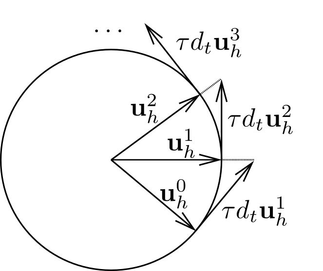
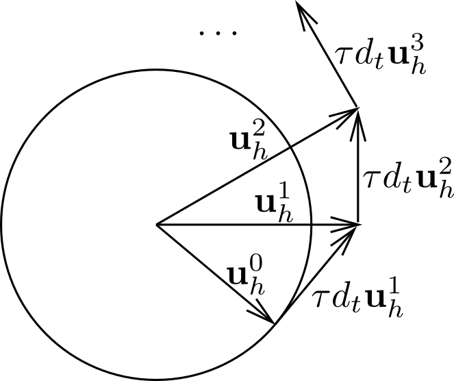
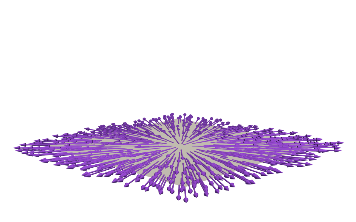
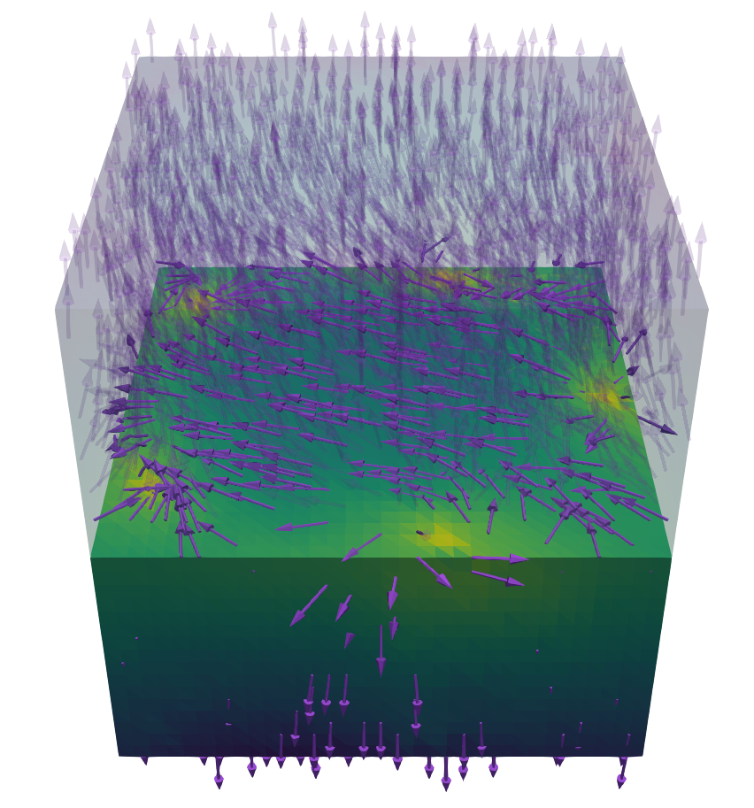
Rigorous convergence analysis for this algorithm for the case of first-order nonconforming discretizations appears in [7, 10]. The original version of the algorithm devised in [3] involved a nodal projection step (Line 1) so that iterates satisfy the sphere constraint exactly in the nodes of the triangulation (Figure 1(a)). In general it is not guaranteed that such a projection step does not increase the energy. Conditions on the triangulation that guarantee an energy decrease during nodal projection limit the applicability of the algorithm in three-dimensional situations [7]. It has been observed in [10] that the projection step can be omitted provided that the time step size $\tau$ tends to zero with the mesh size $h$. In this case the successive violations of the constraint, shown in Figure 1(b), are controlled by the energy of the initial iterate and the step size,

(8) $$\max_{k=0,1,2,\dots}\int_{\Omega}\mathcal{I}^{1}_{h}\big{|}|\mathbf{u}_{h}^{k}|^{2}-1\big{|}\,{\mathrm{d}}x\leq\tau E[\mathbf{u}_{h}^{0}].$$

Remarkably, the maximum violation is independent of the number of iterations, and the bound does not depend on structural properties of the underlying triangulation. This observation even holds for all target manifolds that are given as level sets of suitably regular functions. inline,author=OS,color=green]PPP: [Ref]?

4.2. Riemannian trust-region method

For a provably convergent second-order method we turn to the field of optimization on manifolds [1]. The discrete problem for finding minimizing harmonic maps has the form of a minimization problem for the Dirichlet energy (1) in the discrete admissible set $\mathcal{A}_{h}$. As finite element functions from either discretization are uniquely defined by their values at the Lagrange nodes, the sets $\mathcal{A}_{h}^{\text{proj}}$ and $\mathcal{A}_{h}^{nc}$ are both diffeomorphic to the product manifold $(S^{m-1})^{N}$. Consequently, they are smooth manifolds themselves. In order to solve the minimization problem on $\mathcal{A}_{h}\in\{\mathcal{A}_{h}^{\textup{nc}},\mathcal{A}_{h}^{\textup{proj}}\}$ we employ a Riemannian trust-region method. This algorithm generalizes standard trust-region methods to objective functionals defined on a Riemannian manifold. At a given iterate $\mathbf{v}_{h}^{k}$, it lifts the objective functional from a neighborhood of $\mathbf{v}_{h}^{k}$ in $\mathcal{A}_{h}$ onto the tangent space $T_{h}(\mathbf{v}_{h}^{k})$

$$\hat{E} :T_{h}(\mathbf{v}_{h}^{k})\to\mathbb{R}\qquad\hat{E}(\boldsymbol{\varphi}_{h})\colonequals E[\operatorname{Exp}_{v_{h}^{k}}(\boldsymbol{\varphi}_{h})].$$

Then, it solves a constrained quadratic correction problem on the (linear) tangent space, and maps the result back onto $\mathcal{A}_{h}$. The lifting is realised via the discrete exponential map $\operatorname{Exp}_{\mathbf{v}_{h}}:T_{h}(\mathbf{v}_{h})\to\mathcal{A}_{h}$. It acts by application of the exponential map for the sphere

$$\exp_{x}v=\cos\lvert v\rvert\cdot x+\frac{\sin\lvert v\rvert}{\lvert v\rvert}\cdot v\qquad\text{where $x\in S^{m-1}$ and $v\in T_{x}S^{m-1}$},$$

to each coefficient. The quadratic trust-region subproblem at an iterate $\mathbf{v}_{h}^{k}$ is

(9) $$\min_{\boldsymbol{\varphi}_{h}\in T_{h}(\mathbf{v}_{h}^{k})}\hat{m}_{k}(\boldsymbol{\varphi}_{h}) =\hat{E}[0]+\left\langle\operatorname{grad}\hat{E}[0],\boldsymbol{\varphi}_{h}\right\rangle+\frac{1}{2}\left\langle\operatorname{Hess}\hat{E}[0](\boldsymbol{\varphi}_{h}),\boldsymbol{\varphi}_{h}\right\rangle$$

$$\text{such that}\quad\lVert\boldsymbol{\varphi}_{h}\rVert_{\mathbf{v}_{h}^{k}} \leq\Delta_{k},$$

where $\lVert\cdot\rVert_{v_{h}^{k}}$ is a suitable Riemannian or Finsler norm, and $\Delta_{k}$ is the current trust-region radius. Furthermore, $\operatorname{grad}\hat{E}$ and $\operatorname{Hess}\hat{E}$ denote the Riemannian gradient and Hessian at $\mathbf{v}_{h}^{k}$, respectively. These can be computed from the formulas derived in [2]. For the numerical experiments we use a monotone multigrid (MMG) method to solve the quadratic problems (9). For a detailed description of that method see [38, 31].

Whether the new iterate $\mathbf{v}_{h}^{k+1}=\operatorname{Exp}_{\mathbf{v}_{h}^{k}}(\boldsymbol{\varphi}_{h})$ is actually accepted depends on whether it realizes sufficient energy decrease. This is measured by the ratio of actual and expected energy decrease

(10) $$\rho_{k}\colonequals\frac{E(\operatorname{Exp}_{v_{h}^{k}}(0))-E(\operatorname{Exp}_{v_{h}^{k}}(\boldsymbol{\varphi}_{h}))}{\hat{m}_{k}(0)-\hat{m}_{k}(\boldsymbol{\varphi}_{h})}.$$

This quantity also controls the evolution of the trust-region radius [17].

Input: Initial iterate $\mathbf{v}_{h}^{0}\in\mathcal{A}_{h}$, initial trust-region radius $\Delta_{0}>0$, tolerances $\beta_{1}>\beta_{2}>0$ and stopping criterion $\epsilon_{\mathrm{stop}}>0$

1 for $k=1,2,\dots$ do

2       Solve (9) for $\boldsymbol{\varphi}_{h}\in T_{h}(\mathbf{v}_{h}^{k})$

3       if $(\boldsymbol{\varphi}_{h},\boldsymbol{\varphi}_{h})_{*}<\epsilon_{\mathrm{stop}}^{2}$ then

4             return $\mathbf{v}_{h}^{k}$

5       else

6            

7            Evaluate $\rho_{k}$ from (10)

8            

9            if $\rho_{k}>\beta_{1}$ then

10                   $\mathbf{v}_{h}^{k+1}=\operatorname{Exp}_{\mathbf{v}_{h}^{k}}(\boldsymbol{\varphi}_{h})$ and $\Delta_{k+1}=2\Delta_{k}$

11             else if $\rho_{k}>\beta_{2}$ then

12                   $\Delta_{k+1}=\Delta_{k}$ and $\mathbf{v}_{h}^{k+1}=\operatorname{Exp}_{\mathbf{v}_{h}^{k}}(\boldsymbol{\varphi}_{h})$

13             else

14                   $\Delta_{k+1}=\frac{1}{2}\Delta_{k}$ and $\mathbf{v}_{h}^{k+1}=\mathbf{v}_{h}^{k}$

15                  

16             end if

17            

18       end if

19      

20 end for

Algorithm 2 Riemannian trust-region method

The global convergence of this method to first-order stationary points has been proved by Absil et al. [1]. Moreover, depending on the accuracy of the inner solver, the local convergence is superlinear or even quadratic. We refer to [1] for more details.

5. Benchmarks problems

In this section we present the set of benchmark problems that will serve to test the discretizations and solver algorithms. In the following, $\Omega$ is always the open $n$-dimensional square $(-\frac{1}{2},\frac{1}{2})^{n}$. The first test problem constructs a harmonic map that is $C^{\infty}$ in the domain.

Problem 1 (Smooth harmonic map).

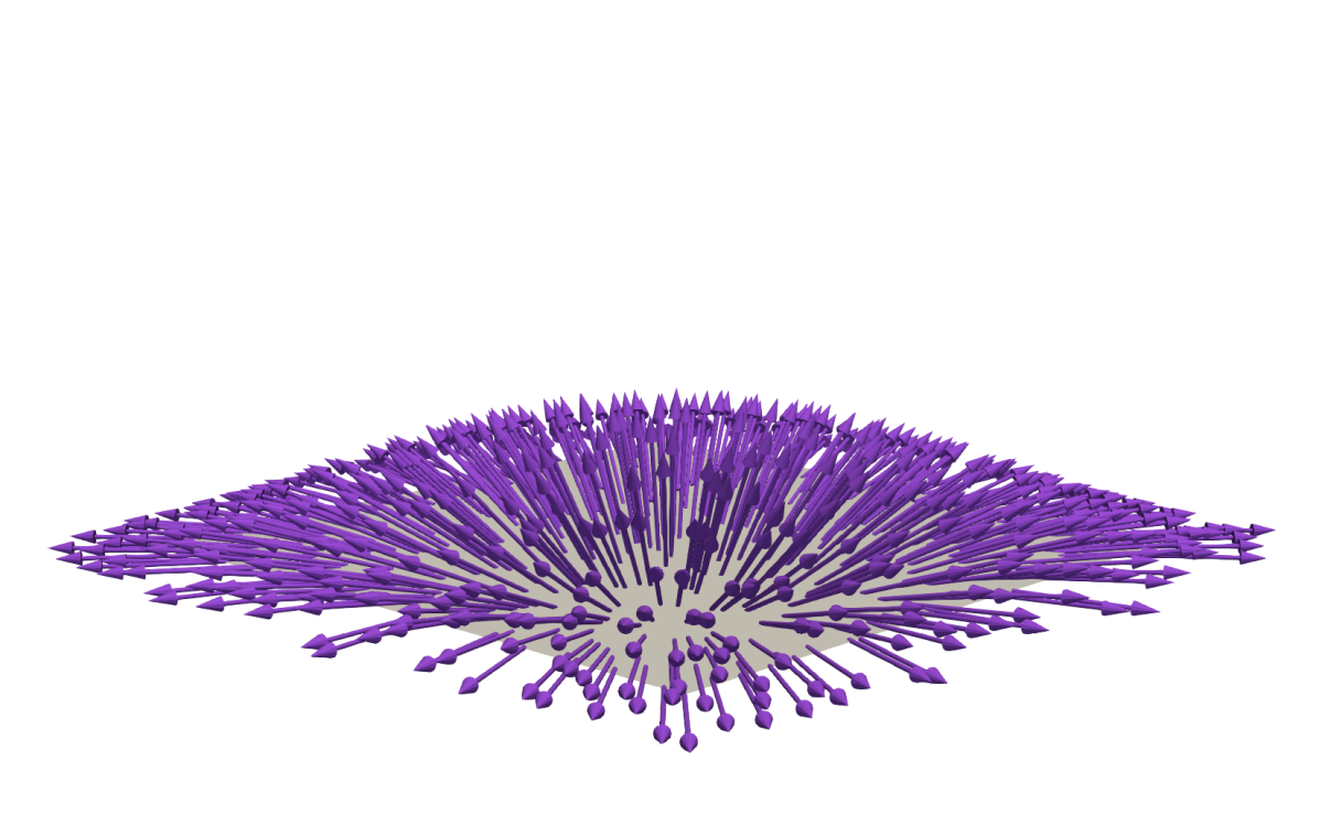
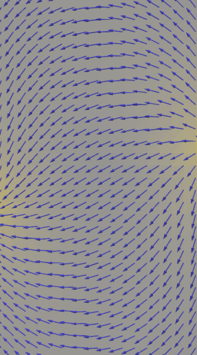
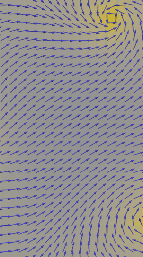
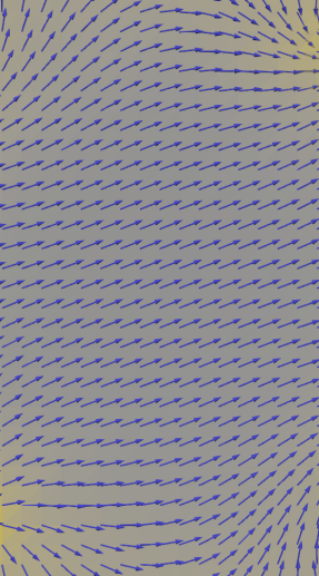
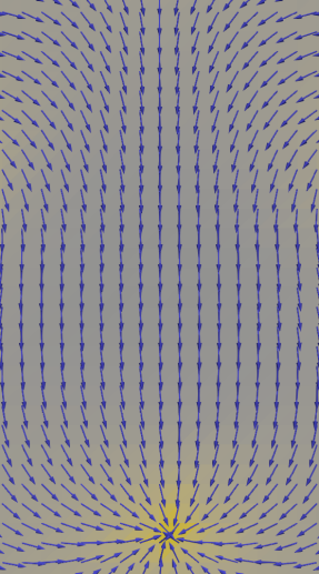
Let $\Omega=(-\frac{1}{2},\frac{1}{2})^{2}$ and set $m=3$, i.e., the image space is $S^{2}$. Compute a harmonic map that agrees with $\mathbf{u}_{D}(x)=\frac{(x_{1},x_{2},0)^{T}}{\lvert x\rvert}$ on the domain boundary. With these boundary conditions, the Dirichlet energy has minimizers in each homotopy class, and the minimizers are $C^{\infty}$. inline,author=OS,color=green]kann man hier ein Existenzresultat zitieren? inline,author=OS,color=green]Referenz inline,author=OS,color=green]Es wäre schlüssiger hier die inverse stereographische Abbildung als Problem zu nehmen – Da hat man die exakte Lösung. A numerical solution for this problem is shown in Figure 2(a).

The next problem computes harmonic maps with a single singularity. We distinguish two cases of differing regularity. Both use the radial projection map

$$\pi(x)\colonequals\frac{x}{\lvert x\rvert}$$

as the boundary condition function.

Problem 2 (Harmonic maps with a singularity).

1. Singular harmonic map with finite energy: If $n=m=3$, the function $\mathbf{u}_{\rm D}(x)=\pi(x)=x/\lvert x\rvert$ minimizes the harmonic energy. The corresponding minimal energy on the unit cube is given by

   $$E[\mathbf{u}_{D}]=6\int\limits_{-\pi/4}^{\pi/2}\frac{\pi-2\arctan(\frac{1}{\sin(\vartheta)})}{\sin(\vartheta)}\,{\mathrm{d}}\vartheta\approx 7.674124,$$

   which can be verified with a computer algebra system. The minimizer $\mathbf{u}_{D}$ is an element of $H^{1}(\Omega;S^{2})$, but not an element of $H^{2}(\Omega;S^{2})$.

2. Singular harmonic map with infinite energy: Let $n=m=2$, i.e., the image space is a circle. In that case, the radial projection $\pi:x\to x/\lvert x\rvert$ is not in $H^{1}(\Omega;S^{1})$ [42, p. 71], and therefore $E[\pi]$ is not well-defined. However, it is still a harmonic map, albeit in the weaker distributional sense.

We quickly prove that $\pi$ is a distributional harmonic map, as this result does not seem to appear in the literature.

Lemma 6.

If $n=m=2$ the radial projection $\pi:x\mapsto\frac{x}{\lvert x\rvert}$ is harmonic in the distributional sense.

Proof.

One directly checks that $\partial_{i}\mathbf{u}$, $i=1,2$, and $-\Delta\mathbf{u}$ are, respectively, perpendicular and parallel to $\mathbf{u}$, which itself coincides with the unit normal $\mathbf{n}$ to the ball $B_{\varepsilon}(0)$ of radius $\varepsilon$ around the origin. With this, a splitting of the integral and two integrations by parts lead to

$$\int_{\Omega}\mathbf{u}\cdot(-\Delta\boldsymbol{\varphi})\,{\mathrm{d}}x= \int_{B_{\varepsilon}(0)}\mathbf{u}\cdot(-\Delta\boldsymbol{\varphi})\,{\mathrm{d}}x-\int_{\partial(\Omega\setminus B_{\varepsilon}(0))}\mathbf{u}\cdot(\nabla\boldsymbol{\varphi}\mathbf{n})\,{\mathrm{d}}s$$

$$+\int_{\partial(\Omega\setminus B_{\varepsilon}(0))}(\nabla\mathbf{u}\mathbf{n})\cdot\boldsymbol{\varphi}\,{\mathrm{d}}s+\int_{\Omega\setminus B_{\varepsilon}(0)}(-\Delta\mathbf{u})\cdot\boldsymbol{\varphi}\,{\mathrm{d}}x,$$

for any $\boldsymbol{\varphi}\in C_{0}^{\infty}(\Omega;\mathbb{R}^{m})$. The first integral on the right-hand side is bounded in terms of $\varepsilon^{2}$, the second integral is bounded in term of $\varepsilon$, the third integral vanishes since $\nabla\mathbf{u}\mathbf{n}=0$, and the fourth integral vanishes because $\mathbf{u}$ is harmonic outside of $B_{\varepsilon}(0)$. ∎

inline,author=OS,color=green]Regularität von $\pi$ in diesem Fall? For more results on the existence of solutions and their classification we refer to [28, 29].

(a) $\mathbb{R}^{2}\supset\Omega\to S^{2}$

(b) $\mathbb{R}^{3}\supset\Omega\to S^{2}$

(c) $\mathbb{R}^{2}\supset\Omega\to S^{1}$

Figure 2. Discrete solutions for Problems 1, 2(a) and 2(b)

Figure 3. Stationary configurations, clipped at the midsurface $x_{3}=0$, of three-dimensional harmonic maps with multiple singularities, obtained with Algorithm 1 with initial singularity degree $\kappa=2,3,4,5$ (left to right). Singularities are located on the mid-surface, which is colored by the Frobenius norm of the discrete solution gradients.

In a further benchmark we investigate harmonic maps with multiple singularities. Recall that if a map $\mathbf{v}\colon\Omega\to S^{2}$ is continuous in a ball $B_{\varepsilon}(x)$ around a point $x\in\Omega$ except at $x$ itself, the degree of this singularity is defined as the topological winding number of $\mathbf{v}|_{\partial B_{\varepsilon}(x)}$ with respect to $x$, see [14]. The following problem also appears in [3].

Problem 3 (Higher degree singularities in $\mathbb{R}^{3}$).

Let $\pi_{\text{st}}\colon S^{2}\to\mathbb{C}$ denote the stereographic projection into the complex plane and define

$$\mathbf{u}_{\rm D}^{\kappa}(x)\colonequals\pi_{\text{st}}^{-1}\circ g_{\kappa}\circ\pi_{\text{st}}\Big{(}\frac{x}{|x|}\Big{)},$$

where $g_{\kappa}(z)\colonequals z^{\kappa}$ with the winding number (or degree) $\kappa\in\mathbb{N}$. inline,author=OS,color=green]Ist $\mathbf{u}_{\rm D}^{\kappa}(x)$ für alle $\kappa\in\mathbb{Z}$ stationärer Punkt der Dirichlet-Energie? inline,author=KB,color=blue!20!white]In [29, p.12] wird erwähnt dass $\mathbf{u}_{\rm D}^{\kappa}(x)$ für $\kappa=2$ "stationary but not (locally) minimizing" ist. The case $\kappa=1$ is identical to Problem 1(a). According to Brezis, Coron, and Lieb [14] (locally) minimizing harmonic maps are not allowed to have singularities of (absolute) degree greater than one. Hence, $\mathbf{u}_{\rm D}^{\kappa}(x)$ is an unstable configuration.

6. Benchmarking the discretizations

The aim of this section is to numerically compare the two discretizations of Section 3 on the benchmark problems defined in Section 5. We solve the algebraic systems using the Riemannian trust-region solver of Section 3.2, and set it to iterate until machine precision is reached. That way, no algebraic constraint violation occurs, and the algebraic error introduced by the iterative nature of the solver remains negligible. The implementation is a hand-written C++  code based on the Dune libraries [12, 41], and the gradients and Hesse matrices of the discrete energy functionals are computed by the automatic differentiation software ADOL-C [46].

In the following we write $\mathbf{u}$ to denote the exact solution of a problem, and $\mathbf{u}_{h}$ for a finite element approximation on a grid of maximal edge length $h$. We measure the experimental orders of convergence (EOC) with respect to the $L^{2}(\Omega;\mathbb{R}^{m})$ norm and the $H^{1}(\Omega;\mathbb{R}^{m})$ halfnorm

$$\mathrm{EOC}^{L^{2}}_{h}\colonequals\log_{2}\left(\frac{\|\mathbf{u}_{2h}-\mathbf{u}\|_{L^{2}}}{\|\mathbf{u}_{h}-\mathbf{u}\|_{L^{2}}}\right)\quad\text{ and }\quad\mathrm{EOC}^{H^{1}}_{h}\colonequals\log_{2}\left(\frac{|\mathbf{u}_{2h}-\mathbf{u}|_{H^{1}}}{|\mathbf{u}_{h}-\mathbf{u}|_{H^{1}}}\right),$$

respectively. When the exact solution $\mathbf{u}$ is unknown we approximate the EOC by

$$\mathrm{EOC}^{L^{2}}_{h}\colonapprox\log_{2}\left(\frac{\|\mathbf{u}_{4h}-\mathbf{u}_{2h}\|_{L^{2}}}{\|\mathbf{u}_{2h}-\mathbf{u}_{h}\|_{L^{2}}}\right),$$

and likewise for $\mathrm{EOC}^{H^{1}}_{h}$. Note that for the nonconforming discretization, the approximate solutions $\mathbf{u}_{h}$ are piecewise polynomial functions, and therefore the EOCs (and the harmonic energy) can be integrated exactly. The projection-based finite elements, however, are not piecewise polynomials, and no exact quadrature formula is known. In lack of anything better we use Gauss–Legendre quadrature of second and sixth order for the harmonic energy and the EOCs, respectively. The question of more appropriate quadrature formulas for geometric finite elements remains open.

For the numerical experiments we employ uniform triangulations $\mathcal{T}_{h}$ of $\Omega\subset\mathbb{R}^{n}$ into simplices, which we label by refinement level $r$. A grid with refinement level $r$ has an element diameter of $h=2^{-r}\sqrt{n}$. With the exception of the multi-singularity example in Section 6.2.3 we compute discrete harmonic maps on up to eight refinement levels if $\Omega\subset\mathbb{R}^{2}$ and up to six refinement levels if $\Omega\subset\mathbb{R}^{3}$. We use the parameters $\Delta_{0}=\frac{1}{2}$, $\delta_{1}=0.9$ and $\delta_{2}=10^{-2}$ for the Riemannian trust-region solver.

6.1. Continuous finite energy harmonic maps

We begin with Problem 1, i.e., the computation of harmonic maps from $\big{(}-\frac{1}{2},\frac{1}{2}\big{)}^{2}$ to $S^{2}$. This situation admits smooth minimizing harmonic maps with finite energy. Since the boundary condition function $\mathbf{u}_{D}$ of Problem 1 is singular in the center of the domain, we use a mollification as the initial iterate. With the scalar function

$$\eta(s)\colonequals\exp\left(\frac{s^{2}}{s^{2}-1}\right),$$

we extend the boundary conditions $\mathbf{u}_{D}(x)=(x/\lvert x\rvert,0)^{\top}$ on $\partial\Omega$ smoothly to the domain $\Omega$ via

(11) $$\tilde{\mathbf{u}}_{D}(x)=\begin{cases}\left(\;0,\;0,\;1\;\right)^{\top}&\text{if }|x|=0,\\ \big{(}\;\big{(}1-\eta(2\lvert x\rvert)^{2}\big{)}^{1/2}\frac{x}{|x|},\;\eta(2\lvert x\rvert)\;\big{)}^{\top}&\text{if }0<|x|<0.5,\\ \big{(}\;\frac{x}{|x|},\;0\;\big{)}^{\top}&\text{if }|x|\geq 0.5.\end{cases}$$

inline,author=OS,color=green]Ein Bild, bitte! We measure the discretization errors for first- and second-order finite elements. The results are shown in Tables 1 and 2. The rates agree with what would be expected for a linear problem, i.e., $\mathcal{O}(h^{p+1})$ for the $L^{2}$-error and $\mathcal{O}(h^{p})$ for the $H^{1}$-error. For the projection-based finite element discretization this has been proven in [24, 27]. The corresponding question for the nonconforming discretization remains open. Tables 1 and 2 also show the discrete energies of the initial iterate and the minimizers for the different grids. These roughly agree—more so for the second-order finite elements. Observe how the minimizing energy increases with increasing mesh refinement for the nonconforming discretization, whereas it decreases for the conforming discretization (except on very coarse grids). The latter would be the expected behavior for nested finite element spaces. However, neither the conforming nor the nonconforming finite elements lead to nested approximation space hierarchies.

		nonconforming				conforming
$r$	$\lvert\mathcal{T}_{h}\rvert$	$E[\mathbf{u}_{h}^{0}]$	$E[\mathbf{u}_{h}]$	$\mathrm{EOC}^{L^{2}}_{h}$	$\mathrm{EOC}^{H^{1}}_{h}$	$E[\mathbf{u}_{h}^{0}]$	$E[\mathbf{u}_{h}]$	$\mathrm{EOC}^{L^{2}}_{h}$	$\mathrm{EOC}^{H^{1}}_{h}$
1	8	$5.171\,57$	$5.171\,57$			$7.500\,36$	$5.528\,24$
2	32	$6.135\,94$	$5.996\,36$			$6.872\,12$	$6.737\,49$
3	128	$6.9523$	$6.2901$	$1.850\,65$	$0.868\,31$	$7.193\,48$	$6.483\,69$	$4.413\,58$	$3.114\,21$
4	512	$7.272\,64$	$6.363\,96$	$2.128\,26$	$0.988\,53$	$7.338\,11$	$6.4129$	$1.9628$	$1.038\,93$
5	2 048	$7.3493$	$6.382\,45$	$2.034\,02$	$0.996\,21$	$7.366\,03$	$6.394\,72$	$1.962\,59$	$1.008\,03$
6	8 192	$7.372\,77$	$6.387\,07$	$2.0077$	$0.998\,97$	$7.376\,98$	$6.390\,14$	$1.987\,18$	$1.001\,98$
7	32 768	$7.378\,75$	$6.388\,22$	$1.997\,63$	$0.999\,74$	$7.3798$	$6.388\,99$	$2.002\,69$	$1.000\,49$
8	131 072	$7.380\,25$	$6.388\,51$	$2.00$	$0.999\,95$	$7.380\,51$	$6.388\,71$	$1.978\,63$	$1.000\,13$

Table 1. Experimental convergence orders for Problem 1, using first-order finite elements

		nonconforming				conforming
$r$	$\lvert\mathcal{T}_{h}\rvert$	$E[\mathbf{u}_{h}^{0}]$	$E[\mathbf{u}_{h}]$	$\mathrm{EOC}^{L^{2}}_{h}$	$\mathrm{EOC}^{H^{1}}_{h}$	$E[\mathbf{u}_{h}^{0}]$	$E[\mathbf{u}_{h}]$	$\mathrm{EOC}^{L^{2}}_{h}$	$\mathrm{EOC}^{H^{1}}_{h}$
1	8	$6.4574$	$6.271\,29$			$6.859\,28$	$6.676$
2	32	$7.224\,41$	$6.383\,99$			$7.362\,92$	$6.414\,73$
3	128	$7.379\,42$	$6.388\,33$	$3.154\,71$	$1.822\,33$	$7.391\,15$	$6.390\,44$	$2.383\,15$	$1.657\,73$
4	512	$7.374\,85$	$6.388\,59$	$2.969\,71$	$1.963\,78$	$7.375\,78$	$6.388\,73$	$3.141\,42$	$1.947\,38$
5	2 048	$7.380\,59$	$6.388\,61$	$2.988\,52$	$1.991\,81$	$7.380\,66$	$6.388\,62$	$3.127\,99$	$1.987\,84$
6	8 192	$7.380\,74$	$6.388\,61$	$2.997$	$1.998$	$7.380\,74$	$6.388\,61$	$3.045\,82$	$1.996\,91$
7	32 768	$7.380\,75$	$6.388\,61$	$2.999\,25$	$1.999\,51$	$7.380\,75$	$6.388\,61$	$3.012\,54$	$1.999\,22$
8	131 072	$7.380\,75$	$6.388\,61$	$1.700\,71$	$1.9997$	$7.380\,75$	$6.388\,61$	$1.683\,69$	$1.999\,56$

Table 2. Experimental convergence orders for Problem 1, using second-order finite elements

6.2. Harmonic maps with a singularity

We repeat the same type of experiment for the two problems 2(a) and 2(b), which both lead to harmonic maps with a singularity.

6.2.1. Singular harmonic map with finite energy

We consider the situation of Problem 2(a) with the boundary condition function $\mathbf{u}_{D}:x\mapsto x/\lvert x\rvert$ on $\partial\Omega$. Recall that this is a problem on a three-dimensional domain, and we therefore measure on fewer different grids. Recall also that the radial projection map $x\mapsto\frac{x}{\lvert x\rvert}$ is in fact harmonic here, and that it is in $H^{1}(\Omega,S^{2})$ but not in $H^{2}(\Omega,S^{2})$. Experimental results are listed in Table 3. For the nonconforming discretization we obtain orders that are a little under $1$ for the $L^{2}$-error and around $0.4$ for the $H^{1}$-error. The $L^{2}$-error is much closer to $1$ for the conforming discretization, but has an outlier at $\approx 0.5$ for the grid with $r=4$. inline,author=OS,color=green]Können wir das irgendwie erklären? The $H^{1}$-error order is nearly $0.5$. Given the regularity of the solution, these convergence orders are what would be expected from the linear theory. However, for a solution that is not continuous, no rigorous results exist currently for either discretization. inline,author=OS,color=green]Eigentlich hätte ich hier gerne auch noch den Fall $p=2$. Again, Table 3 shows the energies of initial iterates and minimizers for the two discretizations. The energies decrease for increasing grid refinement for the conforming discretization (again with one exception), whereas it increases for the nonconforming discretization.

		nonconforming				conforming
$r$	$\lvert\mathcal{T}_{h}\rvert$	$E[\mathbf{u}_{h}^{0}]$	$E[\mathbf{u}_{h}]$	$\mathrm{EOC}^{L^{2}}_{h}$	$\mathrm{EOC}^{H^{1}}_{h}$	$E[\mathbf{u}_{h}^{0}]$	$E[\mathbf{u}_{h}]$	$\mathrm{EOC}^{L^{2}}_{h}$	$\mathrm{EOC}^{H^{1}}_{h}$
1	48	$5.307\,87$	$5.307\,87$			$7.876\,07$	$7.857\,56$
2	384	$6.479\,18$	$6.279\,78$	$1.035\,72$	$0.378\,22$	$8.073\,29$	$7.669\,93$	$1.048\,73$	$0.321\,35$
3	3 072	$7.089\,63$	$6.933\,03$	$0.838\,07$	$0.337\,94$	$7.963\,07$	$7.707\,57$	$1.078\,77$	$0.3982$
4	24 576	$7.386\,13$	$7.290\,99$	$0.836\,75$	$0.362\,23$	$7.841\,07$	$7.717\,13$	$0.512\,75$	$0.534\,42$
5	196 608	$7.531\,43$	$7.479\,08$	$0.8899$	$0.4015$	$7.763\,38$	$7.696\,16$	$0.958\,99$	$0.449\,21$
6	1 572 864	$7.603\,14$	$7.575\,68$	$0.937\,83$	$0.437\,99$	$7.720\,22$	$7.685\,32$	$0.978\,79$	$0.469\,15$

Table 3. Experimental convergence orders for Problem 2(a), using first-order discretizations

6.2.2. Singular harmonic map with infinite energy

In the situation of Problem 2(b) the lack of regularity is even more severe. The radial projection is then a harmonic map in the distributional sense (Lemma 6), but its Dirichlet energy is not a finite number. Nevertheless, the discrete problem is well-defined on each refinement level and it is worthwhile to look for minimizers of the energy in the finite element spaces. Experimental results are shown in Table 4. For both discretizations we still observe linear convergence in the $L^{2}$-sense to the radial projection $x\mapsto\frac{x}{\lvert x\rvert}$. However, in the $H^{1}$-sense there is no convergence at all. The energy of the discrete solutions now grows with increasing refinement levels for both discretizations.

		nonconforming				conforming
$r$	$\lvert\mathcal{T}_{h}\rvert$	$E[\mathbf{u}_{h}^{0}]$	$E[\mathbf{u}_{h}]$	$\mathrm{EOC}^{L^{2}}_{h}$	$\mathrm{EOC}^{H^{1}}_{h}$	$E[\mathbf{u}_{h}^{0}]$	$E[\mathbf{u}_{h}]$	$\mathrm{EOC}^{L^{2}}_{h}$	$\mathrm{EOC}^{H^{1}}_{h}$
1	8	$5.171\,57$	$5.171\,57$			$5.609\,06$	$5.528\,24$
2	32	$7.381\,24$	$6.865\,67$	$0.684\,07$	$-0.004\,53$	$7.890\,83$	$6.793\,58$	$0.682\,59$	$0.200\,39$
3	128	$9.577\,48$	$8.833\,66$	$0.642\,97$	$-0.055\,14$	$10.1041$	$8.791\,02$	$0.824\,57$	$0.025\,88$
4	512	$11.7604$	$10.9553$	$0.784\,54$	$-0.025\,87$	$12.2911$	$10.9424$	$0.877\,92$	$-0.000\,89$
5	2 048	$13.9394$	$13.1187$	$0.848\,57$	$-0.008\,55$	$14.4711$	$13.1143$	$0.897\,37$	$-0.000\,81$
6	8 192	$16.1174$	$15.2927$	$0.880\,01$	$-0.002\,58$	$16.6493$	$15.2905$	$0.910\,22$	$-0.000\,31$
7	32 768	$18.295$	$17.4693$	$0.898\,77$	$-0.000\,75$	$18.827$	$17.4677$	$0.920\,09$	$-0.0001$
8	131 072	$20.4726$	$19.6467$	$0.9117$	$-0.000\,21$	$21.0046$	$19.6452$	$0.928\,06$	$-3\text{\cdot}{10}^{-05}$

Table 4. Experimental convergence orders for Problem 2(b), using first-order discretizations

6.2.3. Decay of higher singularities

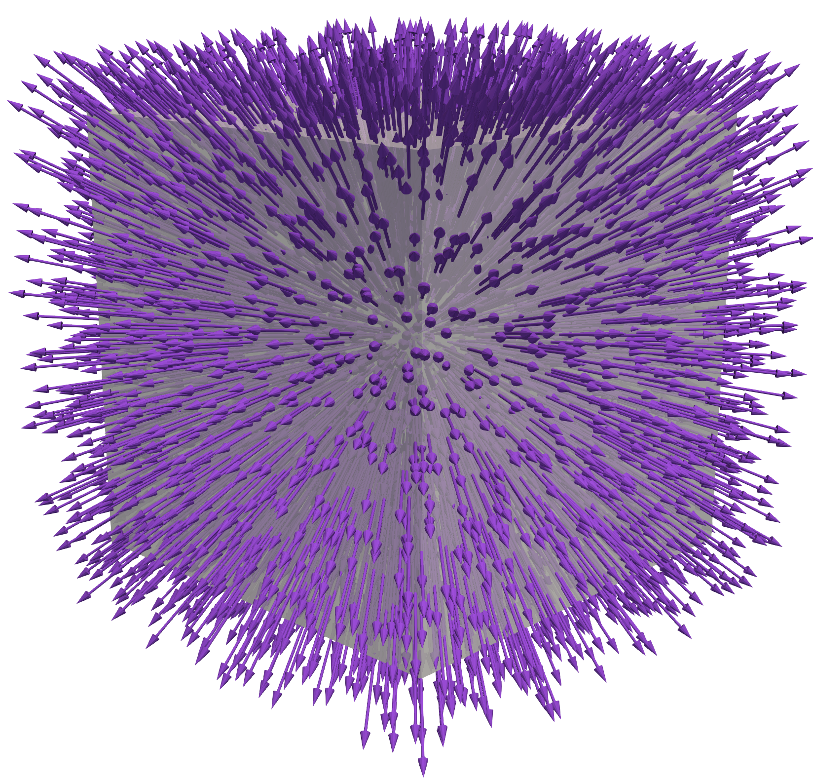
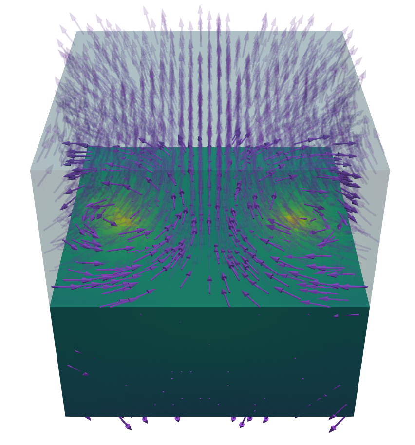
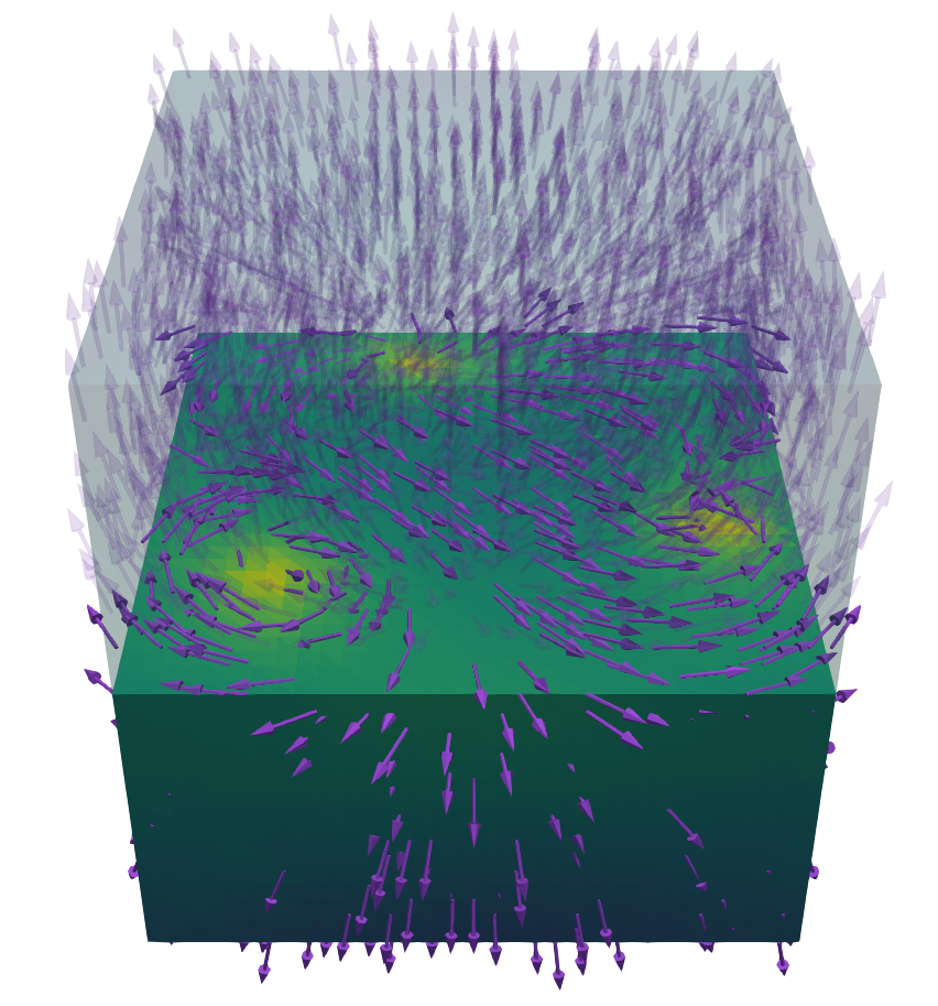
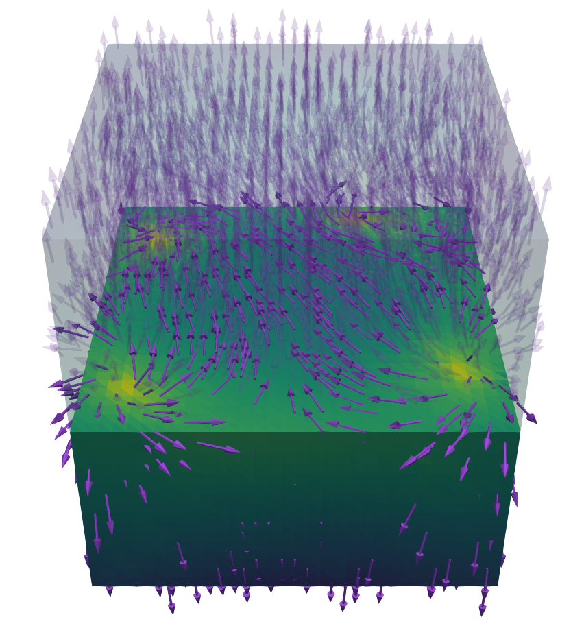
Finally, we compute harmonic maps featuring multiple singularities as described in Problem 3. Using the interpolant of the unstable configuration $\widetilde{\mathbf{u}}^{\kappa}_{D}$ as the initial value in the algorithms, we expect it to decay into several separate singularities of degree $\pm 1$. At the same time we expect the sum of these degrees to be $\kappa$, similar to the results in [3, 16].

(a) Nonconforming discretization

(b) Conforming discretization

Figure 4. Cut through midsurface $x_{3}=0$ for $\kappa=2,\dots,5$ in Problem 3

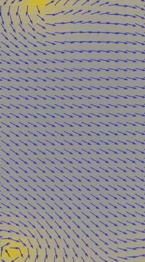
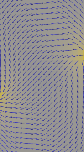
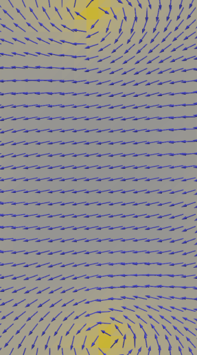
In this example we choose the stopping criterion $\epsilon_{\mathrm{stop}}=10^{-4}$ to limit the simulation times, and compute the resulting approximate minimizers on only five refinement levels. Final configurations are visualized in Figure 4. One can see that the initial singularity has indeed split up into $\kappa$ separate singularities of degree 1. Although all the results admit a certain symmetry, the spatial arrangement of the individual singularities differs depending on the discretization. This is also reflected in a greater deviation between the energy values in Tables 5. The precise reason for this is unclear.

Table 5 also shows the estimated convergence orders for the two discretizations. Unlike in the previous tests, no clear orders are visible in the data for any $\kappa$ and either discretization. This surprising fact requires further investigation. inline,author=OS,color=green]PPP: Das müssen wir klären.

		nonconforming				conforming
$r$	$\lvert\mathcal{T}_{h}\rvert$	$E[\mathbf{u}_{h}^{0}]$	$E[\mathbf{u}_{h}]$	$\mathrm{EOC}^{L^{2}}_{h}$	$\mathrm{EOC}^{H^{1}}_{h}$	$E[\mathbf{u}_{h}^{0}]$	$E[\mathbf{u}_{h}]$	$\mathrm{EOC}^{L^{2}}_{h}$	$\mathrm{EOC}^{H^{1}}_{h}$
		degree $\kappa=2$
1	48	$7.314\,72$	$7.314\,72$			$12.8407$	$12.8194$
2	384	$10.7145$	$9.697\,04$			$15.0622$	$13.3354$
3	3 072	$12.8168$	$11.3129$	$0.639\,65$	$0.4704$	$15.4505$	$13.1777$	$0.689\,82$	$1.3807$
4	24 576	$13.9349$	$12.138$	$0.874\,89$	$0.523\,99$	$15.3633$	$13.2684$	$0.479\,42$	$0.349\,61$
5	196 608	$14.5085$	$12.5099$	$1.013\,91$	$0.433\,54$	$15.2503$	$12.9825$	$0.678\,81$	$0.226\,55$
		degree $\kappa=3$
1	48	$9.028\,58$	$9.028\,58$			$16.1662$	$16.1072$
2	384	$13.9202$	$11.0492$			$21.7559$	$15.1007$
3	3 072	$17.5507$	$13.2049$	$0.475\,93$	$0.269\,91$	$22.9286$	$15.9994$	$0.581\,13$	$0.408\,81$
4	24 576	$19.6904$	$14.3889$	$1.072\,74$	$0.7535$	$22.7473$	$15.7657$	$0.906\,09$	$0.436\,98$
5	196 608	$20.8364$	$14.9595$	$0.862\,75$	$0.274\,47$	$22.4566$	$15.6583$	$0.051\,83$	$0.027\,74$
		degree $\kappa=4$
1	48	$9.783\,71$	$7.783\,71$			$14.5904$	$10.2294$
2	384	$16.1145$	$11.456$			$24.9689$	$17.8951$
3	3 072	$21.4854$	$13.8865$	$0.400\,34$	$-0.059\,85$	$29.1005$	$23.4597$	$0.649\,25$	$-0.704\,38$
4	24 576	$24.9369$	$15.3179$	$0.872\,03$	$0.4943$	$29.6092$	$23.2334$	$0.602\,32$	$0.126\,08$
5	196 608	$26.8608$	$16.0187$	$1.017\,17$	$0.525\,57$	$29.412$	$17.9105$	$0.0298$	$3.9787$
		degree $\kappa=5$
1	48	$9.300\,49$	$9.300\,49$			$16.6115$	$16.593$
2	384	$17.2215$	$12.4729$			$31.1646$	$19.2896$
3	3 072	$24.6533$	$14.6157$	$0.527\,47$	$0.455\,99$	$37.2938$	$18.4116$	$-0.013\,61$	$0.301\,12$
4	24 576	$29.7141$	$16.6423$	$0.572\,87$	$0.123\,07$	$37.7228$	$18.8801$	$1.331\,19$	$0.675\,85$
5	196 608	$32.6394$	$17.5861$	$1.035\,53$	$0.553\,38$	$37.0588$	$18.7542$	$0.555\,21$	$0.294\,36$

Table 5. Experimental convergence orders for Problem 3, using first-order finite elements

7. Benchmarking the solvers

In this second chapter of numerical tests we benchmark the solver algorithms of Chapter 4. In particular, we are interested in solver speed, and how the nonconformity of the gradient solver influences the final result. These questions are not fully decoupled from the choice of discretization. For example, the different finite element spaces seem to influence the problem condition in different ways, and the trust-region solver will typically require fewer iterations for the nonconforming discretization than for the conforming one. Also, the nonconforming gradient solver cannot even be formulated for the conforming discretization of Section 3.2, as that discretization requires all coefficients to have unit length by construction. In this chapter we therefore compare three combinations of solvers and discretizations:

1. The nonconforming gradient flow solver of Section 4.1 for problems discretized with the nonconforming discretization (henceforth abbreviated as Disc(N)/Sol(N)),

2. the Riemannian trust-region solver of Section 4.2 with the nonconforming discretization (Disc(N)/Sol(C)),

3. the Riemannian trust-region solver with the conforming discretization (Disc(C)/Sol(C)).

In order to measure the nodewise violation of the unit-length constraint (2) we introduce the quantity

(12) $$\delta_{1}[\mathbf{u}_{h}]\colonequals\int_{\Omega}\big{|}\mathcal{I}_{h}\left(\lvert\mathbf{u}_{h}\rvert-1\right)\big{|}\,{\mathrm{d}}x.$$

It is closely related to the quantity that appears in the constraint violation bound (8) inline,author=OS,color=green]Post-preprint: Bitte genau die Größe aus (8) nehmen (mit Quadrat). inline,author=OS,color=green]In (8) steht zusätzlich $\max_{k}$. As $\delta_{1}$ is zero for all iterates provided by the Riemannian trust-region method, we show it only for the gradient solver.

For all benchmarks of the trust-region solver we again use the C++/Dune implementation of the previous chapter. The nonconforming gradient solver has been implemented in the Julia language. This difference will only influence the few measurements of wall time we show. As both C++ and Julia are compiled languages we consider this inconsistency acceptable. We set both solvers to iterate until the $(\cdot,\cdot)_{*}$-norm of the correction drops below $\epsilon_{\mathrm{stop}}=10^{-3}$, with the exception of Problem 3 and the test in Section 7.2.2 where $\epsilon_{\mathrm{stop}}=10^{-4}$ is used. inline,author=OS,color=green]PPP: Bitte nach Möglichkeit vereinheitlichen. inline,author=CP,color=teal]In unseren Rechnungen hatten wir überall $10^{-3}$ benutzt in der $H^{1}-Seminorm$. Das $10^{-4}$ hatten wir nur im (nicht mehr vorhandenen) 2-d Fall mal benutzt. For the Riemannian trust-region solver, we set the initial radius to $\Delta_{0}=\frac{1}{2}$, and the parameters of the step acceptance criterion to $\beta_{1}=0.9$ and $\beta_{2}=10^{-2}$. For the tolerance of the inner monotone multigrid solver, a threshold of $\epsilon_{\mathrm{mmg}}=10^{-10}$ is used. For the gradient solver we set the pseudo time step size to four times the grid resolution $\tau=4h$.

7.1. Continuous finite energy harmonic maps

For the first test we again consider Problem 1, where both domain $\Omega=(-\frac{1}{2},\frac{1}{2})^{2}$ and image space $S^{2}$ are two-dimensional. This situation admits smooth minimizing harmonic maps in each homotopy class. We start the solvers from the nodal interpolation of the function (11). inline,author=OS,color=green]PPP: Auf das Bild verweisen sobald es eins gibt.

Table 6 shows the iteration numbers. We observe that the trust-region method only requires $3$ iterations to reach the required accuracy, independent of the grid refinement and the approximation order. inline,author=OS,color=green]Post-Preprint: bitte eine Rechnung für das Gradientenverfahren für eine Diskretisierung zweiter Ordnung. The gradient solver, on the other hand, needs much larger iteration numbers to reach the same accuracy. In fact, starting from the grid $r=3$, the iteration numbers seem to roughly double from one grid to the next-finer one. The difference can be explained by the fact that the trust-region method uses second-order information of the Dirichlet functional (1), whereas the gradient solver does not. Due to the choice of the step size $\tau=4h$, the discrete gradient flow solver requires an increasing amount of iterations for finer and finer grids. The coupling of $\tau$ and $h$, however, is necessary in order to reduce the constraint violation $\delta_{1}$ on smaller mesh sizes according to the estimate (8). Note, however, that gradient-descent iteration are much cheaper than trust-region ones. inline,author=OS,color=green]PPP: Bitte Zeiten für die Rechnung in Table 6, und Diskussion Finally, Table 6 also shows the constraint violation of the minimizers computed by the gradient flow method. They are in the range of $10^{-4}-10^{-3}$, which will be negligible for many practical purposes. In fact, as predicted by (8), the constraint violation is proportional to the time-step size: As we have coupled $\tau$ to be proportional to $h$, the violation is roughly reduced by a factor of $2$ for each grid refinement.

		Disc(N)/Sol(N)		Disc(N)/Sol(C)	Disc(C)/Sol(C)	Disc(N)/Sol(C)	Disc(C)/Sol(C)
		($p=1$)		($p=1$)	($p=1$)	($p=2$)	($p=2$)
$r$	$\lvert\mathcal{T}_{h}\rvert$	#Iter	$\delta_{\mathrm{1}}[\mathbf{u}_{h}]$	#Iter	#Iter	#Iter	#Iter
1	8	1	$5.551\,115\,123\,125\,783\text{\cdot}{10}^{-17}$	1	9	3	3
2	32	13	$0.001\,463\,107\,325\,325\,757\,2$	3	3	3	3
3	128	16	$0.002\,351\,630\,087\,537\,769$	3	3	3	3
4	512	27	$0.001\,422\,808\,572\,953\,798\,6$	3	3	3	3
5	2 048	50	$0.000\,773\,486\,465\,580\,982\,3$	3	3	3	3
6	8 192	94	$0.000\,404\,862\,548\,469\,270\,3$	3	3	3	3
7	32 768	184	$0.000\,207\,229\,901\,213\,026\,75$	3	3	3	3
8	131 072	363	$0.000\,104\,851\,448\,320\,365\,98$	3	3	3	3

Table 6. Iteration numbers and unit-length violation $\delta_{1}$ for Problem 1, using first- and second-order finite elements and a step-size $\tau=4h$

7.2. Harmonic maps with a singularity

In the next sequence of tests we consider harmonic maps with one singularity, to assess how the smoothness of the iterates influences the solver behavior. inline,author=OS,color=green]Zumindest bei den konformen GFE sind ja sogar die FE-Funktionen selbst singulär.

7.2.1. Harmonic map in $H^{1}$

We start with Problem 2(a), which asks for a harmonic map on $(-\frac{1}{2},\frac{1}{2})^{3}$ with image in $S^{2}$. The solution is the radial projection $\pi:x\mapsto\frac{x}{\lvert x\rvert}$, which is singular at the origin, but nevertheless element of $H^{1}$. As a first test we start the solvers directly from the nodal interpolation of the solution. inline,author=OS,color=green]PPP: Ist das ein guter Startwert? Er ist schon sehr nah an der Lösung dran.

Table 7 displays the total number of iterations. Compared to the previous smooth Problem 1, the total number of iterations is slightly increased. However, the qualitative difference between the solvers remain: the number of trust-region iterations remains bounded even for fine grids, whereas the number of gradient flow iterations roughly doubles from one grid to the next. Table 7 also shows the constraint violation $\delta_{1}$ of the gradient flow solver. As in the previous example it decreases with increasing mesh size. In this example, the reduction factor is even better than what is expected from the bound (8).

		Disc(N)/Sol(N)		Disc(N)/Sol(C)	Disc(C)/Sol(C)
$r$	$\lvert\mathcal{T}_{h}\rvert$	#Iter	$\delta_{\mathrm{1}}[\mathbf{u}_{h}]$	#Iter	#Iter
1	48	158	$0.007\,640\,631\,992\,433\,433$	1	6
2	384	184	$0.004\,313\,864\,769\,207\,801$	5	6
3	3 072	95	$0.000\,995\,784\,585\,260\,967\,5$	5	6
4	24 576	246	$0.000\,213\,552\,520\,401\,676\,5$	7	7
5	196 608	445	$4.396\,347\,567\,078\,653\text{\cdot}{10}^{-5}$	6	7
6	1 572 864	923	$7.607\,664\,897\,696\,873\text{\cdot}{10}^{-6}$	6	7

Table 7. Iteration numbers and unit-length violation for Problem 2(a), using first-order finite elements and a time step size of $\tau=4h$

		Disc(N)/Sol(N)	Disc(N)/Sol(C)	Disc(C)/Sol(C)
$r$	$\lvert\mathcal{T}_{h}\rvert$	time [s]	time [s]	time [s]
1	48	$3.209\,912\,247\,999\,999\,7$	$0.937\,704$	$0.166\,739$
2	384	$0.035\,489\,572\,000\,000\,004$	$2.919\,95$	$0.967\,019$
3	3 072	$0.168\,009\,731\,000\,000\,08$	$10.96$	$7.351\,26$
4	24 576	$8.973\,198\,695\,000\,004$	$128.173$	$98.9667$
5	196 608	$524.839\,234\,057\,999\,9$	$1229.58$	$1186$
6	1 572 864	$28\,824.027\,922\,398\,036$	$13\,944.6$	$16\,114.1$

Table 8. Wall-times for Problem 2(a), using first-order finite elements and a time step size of $\tau=4h$

7.2.2. Pseudo-random initial iterate

To challenge the solvers a bit more we simulate Problem 2(a) again, but this time with initial data that is further away from the discrete solution. For this, we replace the previous initial iterate $\mathbf{u}_{h}^{0}(x)=\mathcal{I}_{h}(x/\lvert x\rvert)$ by a (pseudo-)random initial configuration with the same boundary values. Specifically, we consider the following extension $\widetilde{\mathbf{u}}_{D}$ of the boundary conditions

$$\widetilde{\mathbf{u}}_{D}(x)\colonequals\begin{cases}\widetilde{f}(x)&\text{if $x\in\Omega\setminus\partial\Omega$},\\ x/|x|&\text{if $x\in\partial\Omega$},\end{cases}$$

where

$$\widetilde{f}(x_{1},x_{2},x_{3})\colonequals\begin{bmatrix}\sin\left(\frac{\pi}{2}\cdot\sin\Lambda_{1}\right)\cdot\cos\left(\pi\cdot\sin\Lambda_{2}\right)\\ \sin\left(\frac{\pi}{2}\cdot\sin\Lambda_{1}\right)\cdot\sin\left(\pi\cdot\sin\Lambda_{2}\right)\\ \cos\left(\frac{\pi}{2}\cdot\sin\Lambda_{1}\right)\end{bmatrix}$$

and

$$\Lambda_{1}\colonequals 10^{4}x_{1}+10^{5}x_{2}+10^{6}x_{3}\quad\text{ and }\quad\Lambda_{2}\colonequals 5\cdot 10^{4}x_{1}+7\cdot 10^{5}x_{2}+9\cdot 10^{6}x_{3}.$$

Due to the high-frequency character we observe high initial energies that result in a more severe constraint-violation for the discrete gradient flow as well as high iteration numbers, the latter being the reason why we restrict ourselves to coarser grids in this example. inline,author=OS,color=green]PPP: Diskutieren dass wir jetzt ein etwas anderes Ergebnis erhalten. Tun wir das wirklich?

		Disc(N)/Sol(N)		Disc(N)/Sol(C)	Disc(C)/Sol(C)
$r$	$\lvert\mathcal{T}_{h}\rvert$	#Iter	$\delta_{\mathrm{1}}[\mathbf{u}_{h}]$	#Iter	#Iter
1	48	18	$0.085\,185\,365\,008\,552\,12$	1	7
2	384	38	$0.153\,825\,532\,497\,636\,14$	16	21
3	3 072	70	$0.158\,466\,575\,269\,589\,65$	15	22
4	24 576	131	$0.104\,467\,615\,729\,275\,45$	21	18
5	196 608	261	$0.059\,405\,729\,841\,945\,59$	30	54

Table 9. Iteration numbers and unit-length violation for Problem 2(b) with pseudo-random initial iterate, using first-order finite elements and a time step size of $\tau=h$.

7.2.3. Distributional harmonic maps

Next, we investigate Problem 2(b), the approximation of a harmonic map from $(-\frac{1}{2},\frac{1}{2})^{2}$ to $S^{1}$ in the distributional sense. We again start from the nodal interpolation of the solution $x\mapsto\frac{x}{\lvert x\rvert}$. Table 10 shows the total number of iterations as well as the unit-length constraint violation $\delta_{1}$. The number of iterations of both methods is comparable to the case $(-\frac{1}{2},\frac{1}{2})^{3}\to S^{2}$, where the singularity is still in $H^{1}$ (Table 7). However, the nonconforming discretization seems to slightly reduce the number of total iteration steps of the Riemannian trust-region method.

		Disc(N)/Sol(N)		Disc(N)/Sol(C)	Disc(C)/Sol(C)
$r$	$\lvert\mathcal{T}_{h}\rvert$	#Iter	$\delta_{\mathrm{1}}[\mathbf{u}_{h}]$	#Iter	#Iter
1	8	1	$5.551\,115\,123\,125\,783\text{\cdot}{10}^{-17}$	1	4
2	32	15	$0.005\,744\,117\,813\,284\,961$	5	7
3	128	26	$0.001\,919\,558\,788\,314\,368\,5$	5	9
4	512	46	$0.000\,403\,954\,033\,685\,880\,9$	6	9
5	2 048	85	$6.986\,827\,911\,210\,675\text{\cdot}{10}^{-5}$	6	9
6	8 192	163	$1.085\,230\,127\,559\,043\,4\text{\cdot}{10}^{-5}$	6	9
7	32 768	318	$1.583\,475\,603\,411\,615\,5\text{\cdot}{10}^{-6}$	6	9
8	131 072	627	$2.225\,212\,656\,645\,358\,3\text{\cdot}{10}^{-7}$	6	9

Table 10. Iteration numbers and unit-length violation for Problem 2(b), using first-order finite elements and a time step size of $\tau=4h$

7.3. Harmonic maps with multiple singularities

As the final test we measure iteration numbers and constraint violation for the situation with several singularities (Problem 3). The results are shown in Table 11 for up to five singularities. One can see that now even for the trust-region methods the iteration numbers are not bounded anymore, but increase slowly with increasing mesh size. The iteration numbers for the gradient-flow method are again much higher, but do not show a clear pattern as in earlier case. The constraint violation remains in a reasonable range again, and gets smaller with decreasing $\tau=4h$.

		Disc(N)/Sol(N)		Disc(N)/Sol(C)	Disc(C)/Sol(C)
$r$	$\lvert\mathcal{T}_{h}\rvert$	#Iter	$\delta_{\mathrm{1}}[\mathbf{u}_{h}]$	#Iter	#Iter
		degree $\kappa=2$
1	48	51	$0.014\,941\,535\,596\,801\,397$	1	7
2	384	185	$0.013\,390\,237\,061\,175\,923$	11	13
3	3 072	222	$0.007\,774\,474\,414\,193\,014$	12	22
4	24 576	340	$0.002\,662\,653\,356\,781\,558\,4$	16	21
5	196 608	1477	$0.000\,720\,159\,937\,189\,093\,6$	21	50
		degree $\kappa=3$
1	48	78	$0.007\,999\,329\,256\,844\,873$	1	4
2	384	109	$0.032\,974\,361\,166\,974\,08$	12	10
3	3 072	188	$0.018\,030\,437\,535\,823\,115$	12	16
4	24 576	494	$0.006\,459\,695\,356\,191\,741$	17	18
5	196 608	2033	$0.001\,781\,186\,331\,683\,163\,7$	23	44
		degree $\kappa=4$
1	48	17	$0.068\,637\,467\,267\,055\,69$	5	7
2	384	107	$0.048\,214\,028\,390\,724\,56$	10	28
3	3 072	265	$0.030\,490\,452\,242\,260\,05$	14	39
4	24 576	1650	$0.011\,755\,936\,121\,246\,554$	27	46
5	196 608	2045	$0.003\,315\,641\,554\,507\,384\,7$	42	40
		degree $\kappa=5$
1	48	71	$0.008\,993\,154\,163\,545\,151$	1	3
2	384	88	$0.049\,735\,670\,640\,189\,064$	9	10
3	3 072	610	$0.038\,661\,522\,310\,928\,28$	11	17
4	24 576	656	$0.013\,975\,632\,176\,829\,5$	15	37
5	196 608	1381	$0.003\,988\,492\,729\,331\,421$	22	55

Table 11. Iteration numbers and unit-length violation for problem 3, using first-order finite elements and a time step size $\tau=4h$

Acknowledgements The authors gratefully acknowledge the support by the Deutsche Forschungsgemeinschaft in the Research Unit 3013 Vector- and Tensor-Valued Surface PDEs within the sub-projects TP3: Heterogeneous thin structures with prestrain and TP4: Bending plates of nematic liquid crystal elastomers.

References

- [1] P.-A. Absil, R. Mahony, and R. Sepulchre, Optimization algorithms on matrix manifolds, Princeton University Press, 2009.
- [2] P.-A. Absil, R. Mahony, and J. Trumpf, An extrinsic look at the Riemannian Hessian, in International conference on geometric science of information, Springer, 2013, pp. 361–368.
- [3] F. Alouges, A new algorithm for computing liquid crystal stable configurations: The harmonic mapping case, SIAM Journal on Numerical Analysis, 34 (1997), pp. 1708–1726.
- [4] H. Antil, S. Bartels, and A. Schikorra, Approximation of fractional harmonic maps, arXiv preprint arXiv:2104.10049, (2021).
- [5] J. Appell and P. Zabrejko, Nonlinear superposition operators, Cambridge university press, 1990.
- [6] S. Bartels, Robust a priori error analysis for the approximation of degree-one Ginzburg–Landau vortices, ESAIM: Mathematical Modelling and Numerical Analysis, 39 (2005), pp. 863–882.
- [7] S. Bartels, Stability and convergence of finite-element approximation schemes for harmonic maps, SIAM J. Numer. Anal., 43 (2005), pp. 220–238.
- [8] S. Bartels, Numerical analysis of a finite element scheme for the approximation of harmonic maps into surfaces, Mathematics of computation, 79 (2010), pp. 1263–1301.
- [9] S. Bartels, Numerical Methods for Nonlinear Partial Differential Equations, vol. 47 of Springer Series in Computational Mathematics, Springer, 2015.
- [10] , Projection-free approximation of geometrically constrained partial differential equations, Math. Comp., 85 (2016), pp. 1033–1049.
- [11] S. Bartels, M. Griehl, S. Neukamm, D. Padilla-Garza, and C. Palus, A nonlinear bending theory for nematic LCE plates, arXiv e-prints, (2022), p. arXiv:2203.04010.
- [12] P. Bastian, M. Blatt, A. Dedner, N.-A. Dreier, C. Engwer, R. Fritze, C. Gräser, C. Grüninger, D. Kempf, R. Klöfkorn, et al., The Dune framework: Basic concepts and recent developments, Computers & Mathematics with Applications, 81 (2021), pp. 75–112.
- [13] A. Belavin and A. Polyakov, Metastable states of two-dimensional isotropic ferromagnets, JETP lett, 22 (1975), pp. 245–247.
- [14] H. Brezis, J.-M. Coron, and E. H. Lieb, Harmonic maps with defects, Communications in Mathematical Physics, 107 (1986), pp. 649–705.
- [15] P. G. Ciarlet, The finite element method for elliptic problems, SIAM, 2002.
- [16] R. Cohen, R. Hardt, D. Kinderlehrer, S.-Y. Lin, and M. Luskin, Minimum energy configurations for liquid crystals: Computational results, in Theory and Applications of Liquid Crystals, Springer, 1987, pp. 99–121.
- [17] A. Conn, N. Gould, and P. Toint, Trust-Region Methods, SIAM, 2000.
- [18] L. T. de Haan, V. Gimenez-Pinto, A. Konya, T.-S. Nguyen, J. M. Verjans, C. Sánchez-Somolinos, J. V. Selinger, R. L. Selinger, D. J. Broer, and A. P. Schenning, Accordion-like actuators of multiple 3d patterned liquid crystal polymer films, Advanced Functional Materials, 24 (2014), pp. 1251–1258.
- [19] A. DeSimone, R. V. Kohn, S. Müller, and F. Otto, Recent analytical developments in micromagnetics, Preprint 80, Max-Planck-Institut für Mathematik in den Naturwissenschaften, 2004.
- [20] Q. Du, M. D. Gunzburger, and J. S. Peterson, Analysis and approximation of the Ginzburg–Landau model of superconductivity, Siam Review, 34 (1992), pp. 54–81.
- [21] J. Eells and L. Lemaire, Two reports on harmonic maps, World Scientific, 1995.
- [22] E. S. Gawlik and M. Leok, Embedding-based interpolation on the special orthogonal group, SIAM Journal on Scientific Computing, 40 (2018), pp. A721–A746.
- [23] P. Grohs, H. Hardering, and O. Sander, Optimal a priori discretization error bounds for geodesic finite elements, Foundations of Computational Mathematics, 15 (2015), pp. 1357–1411.
- [24] P. Grohs, H. Hardering, O. Sander, and M. Sprecher, Projection-based finite elements for nonlinear function spaces, SIAM Journal on Numerical Analysis, 57 (2019), pp. 404–428.
- [25] H. Hardering, The Aubin–Nitsche trick for semilinear problems, arXiv preprint arXiv:1707.00963, (2017).
- [26] , -discretization error bounds for maps into Riemannian manifolds, Numerische Mathematik, 139 (2018), pp. 381–410.
- [27] H. Hardering and O. Sander, Geometric finite elements, in Handbook of Variational Methods for Nonlinear Geometric Data, Springer, 2020, pp. 3–49.
- [28] F. Hélein, Harmonic maps, conservation laws and moving frames, vol. 150 of Cambridge Tracts in Mathematics, Cambridge University Press, Cambridge, second ed., 2002. Translated from the 1996 French original, With a foreword by James Eells.
- [29] F. Hélein and J. C. Wood, Harmonic maps, Handbook of global analysis, 1213 (2008), pp. 417–491.
- [30] R. R. Kohlmeyer and J. Chen, Wavelength-selective, IR light-driven hinges based on liquid crystalline elastomer composites, Angewandte Chemie, 125 (2013), pp. 9404–9407.
- [31] R. Kornhuber, Adaptive monotone multigrid methods for nonlinear variational problems, Vieweg+ Teubner Verlag, 1997.
- [32] S.-Y. Lin, Numerical analysis for liquid crystal problems, University of Minnesota, 1987.
- [33] C. Liu and N. J. Walkington, Approximation of liquid crystal flows, SIAM Journal on Numerical Analysis, 37 (2000), pp. 725–741.
- [34] C. Melcher, Chiral skyrmions in the plane, Proc. of the Royal Society A, (2014). online, DOI: 10.1098/rspa.2014.0394.
- [35] A. Monteil, R. Rodiac, and J. Van Schaftingen, Ginzburg–Landau relaxation for harmonic maps on planar domains into a general compact vacuum manifold, Archive for Rational Mechanics and Analysis, 242 (2021), pp. 875–935.
- [36] R. H. Nochetto, S. W. Walker, and W. Zhang, A finite element method for nematic liquid crystals with variable degree of orientation, SIAM J. Numer. Anal., 55 (2017), pp. 1357–1386.
- [37] O. Sander, Geodesic finite elements for Cosserat rods, International Journal for Numerical Methods in Engineering, 82 (2010), pp. 1645–1670.
- [38] , Geodesic finite elements on simplicial grids, Internat. J. Numer. Methods Engrg., 92 (2012), pp. 999–1025.
- [39] , Geodesic finite elements of higher order, IMA J. Numer. Anal., 36 (2016), pp. 238–266.
- [40] , Test function spaces for geometric finite elements, arXiv preprint arXiv:1607.07479, (2016).
- [41] , DUNE—The Distributed and Unified Numerics Environment, vol. 140, Springer Nature, 2020.
- [42] M. Struwe and M. Struwe, Variational methods, vol. 991, Springer, 2000.
- [43] D. J. Thouless, Topological quantum numbers in nonrelativistic physics, World Scientific, 1998.
- [44] L. A. Vese and S. J. Osher, Numerical methods for p-harmonic flows and applications to image processing, SIAM Journal on Numerical Analysis, 40 (2002), pp. 2085–2104.
- [45] S. W. Walker, A finite element method for the generalized Ericksen model of nematic liquid crystals, ESAIM Math. Model. Numer. Anal., 54 (2020), pp. 1181–1220.
- [46] A. Walther and A. Griewank, Getting started with ADOL-C, In U. Naumann and O. Schenk, editors, Combinatorial Scientific Computing, (2012), p. 181–202.
- [47] T. H. Ware, J. S. Biggins, A. F. Shick, M. Warner, and T. J. White, Localized soft elasticity in liquid crystal elastomers, Nature communications, 7 (2016), pp. 1–7.
- [48] A. Weinmann, L. Demaret, and M. Storath, Total variation regularization for manifold-valued data, SIAM Journal on Imaging Sciences, 7 (2014), pp. 2226–2257.
- [49] T. J. White and D. J. Broer, Programmable and adaptive mechanics with liquid crystal polymer networks and elastomers, Nature materials, 14 (2015), p. 1087.