A generalized framework for direct discontinuous Galerkin methods for nonlinear diffusion equations

Abstract

In this study, we propose a unified, general framework for the direct discontinuous Galerkin methods. In the new framework, the antiderivative of the nonlinear diffusion matrix is not needed. This allows a simple definition of the numerical flux, which can be used for general diffusion equations with no further modification. We also present the nonlinear stability analyses of the new direct discontinuous Galerkin methods and perform several numerical experiments to evaluate their performance. The numerical tests show that the symmetric and the interface correction versions of the method achieve optimal convergence and are superior to the nonsymmetric version, which demonstrates optimal convergence only for problems with diagonal diffusion matrices but loses order for even degree polynomials with a non-diagonal diffusion matrix. Singular or blow up solutions are also well captured with the new direct discontinuous Galerkin methods.

65M12, 65M60

1 Introduction

In this paper, we continue to study direct discontinuous Galerkin method [31] and other three versions of the direct discontinuous Galerkin (DDG) method [32, 41, 43] for solving the nonlinear diffusion equation

(1) $$\frac{\partial U}{\partial t}=\nabla\cdot(A(U)\nabla U),\hskip 14.22636pt(\textbf{x},t)\in\Omega\times(0,T),$$

with the initial data $U_{0}(\textbf{x})=U(\textbf{x},0)$. Nonlinear diffusion matrix $A(U)\in\mathbb{R}^{d\times d}$ is assumed to be positive definite. We adapt $\Omega\subset\mathbb{R}^{d}$ to denote the computational domain. In this study, we consider a 2-dimensional setting with $d=2$. Our focus is to derive a generalized and unified DDG method for nonlinear diffusion equations (1) that can be easily extended and applied to system and multi dimensional cases.

The discontinuous Galerkin (DG) method was first introduced by Reed and Hill for neutron transport equations in 1973 [35]. However, it is after a series of papers by Cockburn, Shu et al. [19, 18, 16, 21] that the DG method became the archetype of high order methods used in the scientific community. Essentially, the DG method is a finite element method, but with a discontinuous piecewise polynomial space defined for the numerical solution and test function in each element. Due to this property, the DG method has a smaller and more compact stencil compared to its continuous counterpart. Hence, the data structure required to implement DG methods is extremely local, which allows efficient parallel computing and $hp$-adaptation.

One of the key features of the DG method is that the communication between computational elements is established through a numerical flux defined at element interfaces. In this regard, the DG method bears a striking similarity to finite volume method, where a Riemann solver is employed to calculate the numerical flux. Therefore, the DG method enjoys the high-order polynomial approximations as a finite element method while benefiting from the characteristic decomposition of the wave propagation provided by Riemann solvers as a finite volume method. For this reason, the DG method has been successfully applied to hyperbolic problems, i.e. compressible Euler equations, in the last three decades, cf. [17, 38, 48].

On the other hand, for elliptic and parabolic problems, i.e. linear/nonlinear diffusion equations, the numerical flux must involve a proper definition for the solution gradient at element interfaces. It is, in fact, the variety of this definition that leads to several DG methods such as the interior penalty (IPDG) methods [1, 42, 3], the nonsymmetric interior penalty (NIPG) method [36, 37] and the symmetric interior penalty (SIPG) method [27, 26, 28]. Another important group of DG methods for solving diffusion problems include the method of Bassi and Rebay (BR) and its variations [5, 6, 7, 4]; the local DG (LDG) method [20, 14, 44]; the method of Baumann and Oden (BO) [8, 9]; hybridized DG (HDG) method [15]. Recent works include the weakly over-penalized SIPG method [10]; weak DG [30] method and ultra weak DG method [13, 11]. For a review of these methods, we refer to [2, 39] and the references therein. Among the many DG methods mentioned, there is little discussion of nonlinear diffusion equations except Bassi and Rebay [5] and Local DG related methods [20, 15].

In addition to all the efforts mentioned above to devise a numerical flux for the diffusive terms in elliptic/parabolic equations, Liu and Yan [31] introduced Direct DG (DDG) method for nonlinear diffusion equations. Inspired by the exact trace formula corresponding to the solution of heat equation with a smooth initial data that contains a discontinuous point, Liu and Yan derived a simple formula for the numerical flux to compute the solution derivative at the element interface. Although DDG method is proven to converge to the exact solution optimally when measured in an energy norm, it suffers from an order loss in the $L_{2}$-norm when the solution space is approximated by even degree polynomials. In order to recover optimal convergence, Liu and Yan [32] developed the direct DG method with interface correction (DDGIC). In their subsequent studies, Yan and collaborators presented symmetric and nonsymmetric versions of the DDG method [41, 43]. Even though DDG methods degenerate to the IPDG method with piecewise constant and linear polynomial approximations, there exist a number of advantages with DDG methods for higher order approximations. For such advantages, we refer to the discussions on a third order bound preserving scheme in [12], superconvergence to $\nabla U$ in [45, 34] and elliptic interface problems with different jump interface conditions in [29].

Despite the aforementioned favorable features, in the previous versions of DDG methods, the numerical flux definition is based on the antiderivative of the nonlinear diffusion matrix $A(U)$. However, this antiderivative might not exist if the diffusion matrix $A(U)$ is complicated enough. Therefore, the previous DDG methods are not applicable to nonlinear equations with such diffusion matrices. One important example where the diffusion matrix $A(U)$ cannot be integrated explicitly is the energy equation of compressible Navier-Stokes equations. A similar difficulty arises for the interface terms involving test function. This problem is addressed by defining a new direction vector on element interfaces, which depends on the nonlinear diffusion matrix $A(U)$ and geometric information of the interface. With the introduction of the nonlinear direction vector, the evaluation of the nonlinear numerical flux is greatly simplified. Interface terms can also be clearly defined with no ambiguity. Danis and Yan recently applied the method in [22] to solve compressible Navier-Stokes equations with DDGIC method. This treatment of a generic diffusion process opens up the possibility of a straightforward extension of all DDG versions to the complicated nonlinear diffusion equations, which motivates this study.

In this paper, the concept of the nonlinear direction vector is extended to all versions of DDG method in a generalized, unified framework. The new framework does not only address the problem of calculating the antiderivative of the diffusion matrix, but also provides an easy and practical recipe for using the DDG methods for general system of conservation laws. Moreover, interface terms of all versions of DDG methods are presented within a unified format that is clean and easy to be evaluated. Nonlinear stability analyses are presented for the new DDGIC, symmetric DDG and nonsymmetric DDG methods, and we investigate their performance in several numerical experiments. Since DDG methods degenerate to the IPDG method with low order approximations as mentioned, all numerical tests are conducted with high order polynomial approximations. In the numerical tests, optimal order of accuracy are obtained for DDGIC and symmetric DDG methods over uniform triangular meshes while a slight fraction of order loss is observed for nonsymmetric DDG method with even degree polynomial approximations. It is also shown that singular or blow up phenomena can be well captured under the new DDG framework.

Throughout the paper, we denote the exact solution of Equation 1 by the uppercase $U$ and the DG solution of Equation 1 by the lowercase $u$. The rest of the paper is organized as follows. In Section 2, we briefly review the direct DG methods. In Section 3, the new methodology is described. In Section 4, nonlinear stability analysis are presented. Implementation details of the new methods are explained and several numerical examples are presented in Section 5. Finally, we draw our conclusions in Section 6.

2 A review of direct DG methods

In this section, we will present a brief review of the original direct DG methods [31, 32, 41, 43] and the required notation for later use.

We consider a shape regular triangular mesh partition $\mathcal{T}_{h}$ of $\Omega$ such that $\overline{\Omega}=\cup_{{K\in\mathcal{T}_{h}}}K$. For each element $K$, we denote the diameter of the inscribed circle by $h_{K}$. Furthermore, we define the numerical solution space as

$$\mathbb{V}_{h}^{k}:=\{v\in L^{2}(\Omega):v(x,y)\vline_{K}\in\mathbb{P}_{k}(K)\},$$

where $\mathbb{P}_{k}(K)$ represents the space of polynomials of degree $k$ in two dimensions. Note that this solution space is discontinuous across element interfaces. For this purpose, we adopt the following notation for the interface solution jump and average

$$\llbracket u\rrbracket=u^{+}-u^{-},\hskip 28.45274pt\{\!\!\{u\}\!\!\}=\frac{u^{+}+u^{-}}{2},\quad\forall(x,y)\in\partial K,$$

where $u^{+}$ and $u^{-}$ are the solution values calculated from the exterior and interior of the element $K$.

Next, for a test function $v\in\mathbb{V}_{h}^{k}$, we multiply Equation 1 by $v$, integrate it by parts and apply the divergence theorem to obtain the weak form of Equation 1. Along with the initial projection, the weak form is then given by

(2) $$\int_{K}u_{t}v~{}dxdy+\int_{K}A(u)\nabla u\cdot\nabla v~{}dxdy-\int_{\partial K}\widehat{A(u)\nabla u}\cdot\mathbf{n}\,v~{}ds=0,\quad\forall v\in\mathbb{V}_{h}^{k},$$

(3) $$\int_{K}u(x,y,0)v(x,y)~{}dxdy=\int_{K}U_{0}(x,y)v(x,y)~{}dxdy,\quad\forall v\in\mathbb{V}_{h}^{k}.$$

In Equation 2, the volume integration is performed over individual elements $K$ and the surface integral is performed over the element boundary $\partial K$. Here, $\mathbf{n}$ is the outward unit normal vector on $\partial K$. Furthermore, since $u(x,y,t)|_{K}$ is a discontinuous across the elements, $A(u)\nabla u$ is multi-valued on $\partial K$. For this reason, $A(u)\nabla u$ is written with a hat in the surface integral term in Equation 2. In fact, $\widehat{A(u)\nabla u}$ is known as the numerical flux. The original DDG method [31] defines the numerical flux as

(4) $$\widehat{a_{ij}(u)u_{x_{j}}}=\frac{\beta_{0}}{h_{e}}\llbracket b_{ij}(u)\rrbracket n_{j}+\{\!\!\{b_{ij}(u)_{x_{j}}\}\!\!\}+\beta_{1}h_{e}\llbracket b_{ij}(u)_{x_{1}x_{j}}n_{1}+b_{ij}(u)_{x_{2}x_{j}}n_{2}\rrbracket,$$

where we denote by $a_{ij}(u)$ the $ij$ component of the diffusion matrix $A(u)$. Here, $b_{ij}(u)$ are the components of the matrix $B(u)$. Basically, the components of $B(u)$ are the antiderivatives of $a_{ij}(u)$ and it is defined as $b_{ij}(u)=\int^{u}a_{ij}(s)ds$. In Equation 4, $h_{e}$ is the average of the element diameters sharing the edge $\partial K$, $n_{j}$ are the components of the unit normal $\mathbf{n}$ for $j=1,2$, and the subscripts $x_{j}$ denote the partial derivative with respect to the corresponding spatial coordinate axis for $j=1,2$. Furthermore, $(\beta_{0},\beta_{1})$ is a pair of coefficients that affects the stability and optimal convergence of the DDG method. Along with Equations 2 and 4, the definition of the original direct DG method [31] is now completed.

It is well-known that the original DDG method loses an order for even degree polynomials [31]. This problem is fixed either by including a jump term for the test function or introducing a numerical flux for the test function. What determines the name of the corresponding DDG version is in fact how these additional terms are implemented.

2.1 The DDG method with interface correction

The scheme formulation of the original DDGIC method [32] is given as

$$\int_{K}u_{t}v~{}dxdy +\int_{K}A(u)\nabla u\cdot\nabla v~{}dxdy$$

$$-\int_{\partial K}\widehat{A(u)\nabla u}\cdot\mathbf{n}\,v~{}ds+\int_{\partial K}\llbracket B(u)\rrbracket\{\!\!\{\nabla v\}\!\!\}\cdot\mathbf{n}~{}ds=0,\quad\forall v\in\mathbb{V}_{h}^{k},$$

where the numerical flux $\widehat{A(u)\nabla u}$ is calculated using Equation 4. Note that the test function $v$ is only nonzero inside the element $K$ by definition, thus the interface correction term is calculated as

$$\llbracket B(u)\rrbracket\{\!\!\{\nabla v\}\!\!\}=\frac{1}{2}\llbracket B(u)\rrbracket(\nabla v)^{-}.$$

2.2 The symmetric DDG method

The scheme formulation of the original symmetric DDG method [41] is given by

$$\int_{K}u_{t}v~{}dxdy +\int_{K}A(u)\nabla u\cdot\nabla v~{}dxdy$$

$$-\int_{\partial K}\widehat{A(u)\nabla u}\cdot\mathbf{n}\,v~{}ds+\int_{\partial K}\llbracket B(u)\rrbracket\widehat{\nabla v}\cdot\mathbf{n}~{}ds=0,\quad\forall v\in\mathbb{V}_{h}^{k}.$$

As in the DDGIC method, the numerical flux $\widehat{A(u)\nabla u}$ is calculated by Equation 4 while the numerical for the test function is given as

(5) $$\widehat{v}_{x} =\beta_{0}\frac{\llbracket v\rrbracket}{h_{e}}n_{1}+\{\!\!\{v_{x}\}\!\!\}+\beta_{1}h_{e}\llbracket v_{xx}n_{1}+v_{yx}n_{2}\rrbracket,$$

$$\widehat{v}_{y} =\beta_{0}\frac{\llbracket v\rrbracket}{h_{e}}n_{2}+\{\!\!\{v_{y}\}\!\!\}+\beta_{1}h_{e}\llbracket v_{xy}n_{1}+v_{yy}n_{2}\rrbracket.$$

Note that the test function is zero outside of the element $K$. Thus, Equation 5 can be simplified as

$$\widehat{v}_{x} =-\beta_{0}\frac{v^{-}}{h_{e}}n_{1}+\frac{1}{2}v_{x}^{-}-\beta_{1}h_{e}\left(v_{xx}^{-}n_{1}+v_{yx}^{-}n_{2}\right),$$

$$\widehat{v}_{y} =-\beta_{0}\frac{v^{-}}{h_{e}}n_{2}+\frac{1}{2}v^{-}_{y}-\beta_{1}h_{e}\left(v^{-}_{xy}n_{1}+v^{-}_{yy}n_{2}\right).$$

2.3 The nonsymmetric DDG method

The scheme formulation of the original nonsymmetric DDG method [43] is given by

$$\int_{K}u_{t}v~{}dxdy +\int_{K}A(u)\nabla u\cdot\nabla v~{}dxdy$$

$$-\int_{\partial K}\widehat{A(u)\nabla u}\cdot\mathbf{n}\,v~{}ds-\int_{\partial K}\widetilde{A(v)\nabla v}\cdot\mathbf{n}\llbracket u\rrbracket~{}ds=0,\quad\forall v\in\mathbb{V}_{h}^{k}.$$

Similar to the other DDG versions, the numerical flux $\widehat{A(u)\nabla u}$ is calculated by Equation 4. The numerical flux for the test function is defined similarly but with a different penalty coefficient $\beta_{0v}$:

(6) $$\widetilde{a_{ij}(v)v_{x_{j}}}=\frac{\beta_{0v}}{h_{e}}\llbracket b_{ij}(v)\rrbracket n_{j}+\{\!\!\{b_{ij}(v)_{x_{j}}\}\!\!\}+\beta_{1}h_{e}\llbracket b_{ij}(v)_{x_{1}x_{j}}n_{1}+b_{ij}(v)_{x_{2}x_{j}}n_{2}\rrbracket.$$

Since the test function is undefined outside of the element $K$, Equation 6 can be simplified as

$$\widetilde{a_{ij}(v)v_{x_{j}}}=-\frac{\beta_{0v}}{h_{e}}b_{ij}(v^{-})n_{j}+\frac{1}{2}b_{ij}(v^{-})_{x_{j}}-\beta_{1}h_{e}\left(b_{ij}(v^{-})_{x_{1}x_{j}}n_{1}+b_{ij}(v^{-})_{x_{2}x_{j}}n_{2})\right).$$

3 The new DDG framework for nonlinear diffusion equations

As can be seen in the previous section, the numerical flux definition of original DDG versions is based on calculating an antiderivative matrix $B(u)$ that is calculated according to

$$B(u)=\int^{u}A(s)ds.$$

A major drawback occurs when the components of the diffusion matrix $A(u)$ cannot be integrated explicitly. In such cases, none of the original DDG versions can be implemented. A striking example is the energy equation of compressible Navier-Stokes equations. This drawback limits the use of the original DDG versions only to simple applications where the antiderivative matrix $B(u)$ is available.

The new framework is based on the adjoint-property of inner product, which was used in the proof of a bound-preserving limiter with DDGIC method [12]. On the continuous level, the integrand of the surface integral in the weak form Equation 2 can be rewritten as

$$A(u)\nabla u\cdot\mathbf{n}=\nabla u\cdot A(u)^{T}\mathbf{n}.$$

By applying the adjoint-property, we define a new direction vector $\boldsymbol{\xi}(u)=A(u)^{T}\mathbf{n}$. The new direction vector is simply obtained by stretching/compressing and rotating the unit normal vector $\mathbf{n}$ through diffusion matrix $A(u)$. On the discrete level, the new direction vector can be calculated by

(7) $$\boldsymbol{\xi}\left(\{\!\!\{u\}\!\!\}\right)=A(\{\!\!\{u\}\!\!\})^{T}\mathbf{n}.$$

The numerical flux can suitably be defined as

$$\widehat{A(u)\nabla u}\cdot\mathbf{n}=\widehat{\nabla u}\cdot\boldsymbol{\xi}\left(\{\!\!\{u\}\!\!\}\right),$$

where the numerical flux $\widehat{\nabla u}=(\widehat{u}_{x},\widehat{u}_{y})$ can be computed by the original DDG numerical flux formula for the heat equation [31]:

(8) $$\widehat{u}_{x} =\beta_{0}\frac{\llbracket u\rrbracket}{h_{e}}n_{1}+\{\!\!\{u_{x}\}\!\!\}+\beta_{1}h_{e}\llbracket u_{xx}n_{1}+u_{yx}n_{2}\rrbracket,$$

$$\widehat{u}_{y} =\beta_{0}\frac{\llbracket u\rrbracket}{h_{e}}n_{2}+\{\!\!\{u_{y}\}\!\!\}+\beta_{1}h_{e}\llbracket u_{xy}n_{1}+u_{yy}n_{2}\rrbracket.$$

Now, we reformulate all DDG versions for Equation 1 according to the new framework: Find $u\in\mathbb{V}_{h}^{k}$ such that

(9) $$\int_{K}u_{t}v~{}dxdy +\int_{K}A(u)\nabla u\cdot\nabla v~{}dxdy$$

$$-\int_{\partial K}\widehat{\nabla u}\cdot\boldsymbol{\xi}(\{\!\!\{u\}\!\!\})v~{}ds+\sigma\int_{\partial K}\llbracket u\rrbracket\widetilde{\nabla v}\cdot\boldsymbol{\xi}(\{\!\!\{u\}\!\!\})~{}ds=0,\quad\forall v\in\mathbb{V}_{h}^{k},$$

where $\sigma=0$ for the basic DDG scheme, $\sigma=1$ for DDGIC and symmetric DDG schemes, and $\sigma=-1$ for the nonsymmetric DDG scheme. Furthermore, we denote by $\widetilde{\nabla v}$ the numerical flux for the test function $v\in\mathbb{V}_{h}^{k}$. Along with the following definitions of the numerical flux for the test function, Equation 9 defines the new DDG versions:

The baseline DDG scheme ($\sigma=0$):

(10) $$\widetilde{\nabla v}=\mathbf{0}.$$

The DDGIC scheme ($\sigma=1$):

(11) $$\widetilde{\nabla v}=\{\!\!\{\nabla v\}\!\!\}.$$

The symmetric DDG scheme ($\sigma=1$):

(12) $$\widetilde{v}_{x} =\beta_{0}\frac{\llbracket v\rrbracket}{h_{e}}n_{1}+\{\!\!\{v_{x}\}\!\!\}+\beta_{1}h_{e}\llbracket v_{xx}n_{1}+v_{yx}n_{2}\rrbracket,$$

$$\widetilde{v}_{y} =\beta_{0}\frac{\llbracket v\rrbracket}{h_{e}}n_{2}+\{\!\!\{v_{y}\}\!\!\}+\beta_{1}h_{e}\llbracket v_{xy}n_{1}+v_{yy}n_{2}\rrbracket.$$

The nonsymmetric DDG scheme ($\sigma=-1$):

(13) $$\widetilde{v}_{x} =\beta_{0v}\frac{\llbracket v\rrbracket}{h_{e}}n_{1}+\{\!\!\{v_{x}\}\!\!\}+\beta_{1}h_{e}\llbracket v_{xx}n_{1}+v_{yx}n_{2}\rrbracket,$$

$$\widetilde{v}_{y} =\beta_{0v}\frac{\llbracket v\rrbracket}{h_{e}}n_{2}+\{\!\!\{v_{y}\}\!\!\}+\beta_{1}h_{e}\llbracket v_{xy}n_{1}+v_{yy}n_{2}\rrbracket.$$

In [12], the adjoint property of inner product was only used in the proof of positivity-preserving (Theorem 3.2). All numerical tests of [12] involving nonlinear diffusion equations were implemented with the original DDGIC scheme formulation [32].

Remark 3.1.

We summarize the main features and advantages of the generalized DDG methods (9) for nonlinear diffusion equation (1).

• Nonlinearity of the diffusion process goes into the corresponding new direction vector defined at the cell interface that greatly simplifies the implementation of the DDG method.

• Numerical flux for the solution’s gradient $\nabla u$ can be approximated by the linear numerical flux formula of the original DDG. Since the solution’s gradient is independent of the governing equation, this allows the code reuse for general nonlinear diffusion problems.

• The nonlinear direction vectors are further applied to define the interface terms involving test function.

4 Nonlinear stability of the new DDG methods

In this section, we will discuss the nonlinear stability theory of the DDG methods developed in Section 3. The important inequalities used in the proofs of the main theorems are discussed later in Appendix A.

We say that the DDG method is stable in $L_{2}$ sense if

$$\int_{\Omega}u^{2}(x,y,T)~{}dxdy\leq\int_{\Omega}U^{2}_{0}(x,y)~{}dxdy,\quad\forall T\geq 0.$$

Note that the primal weak formulation of the new DDG methods is obtained by summing Equations 3 and 9 over all element $K\in\mathcal{T}_{h}$.

(14) $$\int_{\Omega}u_{t}v~{}dxdy+\mathbb{B}(u,v)=0,\quad\forall v\in\mathbb{V}_{h}^{k}.$$

(15) $$\int_{\Omega}u(x,y,0)v(x,y)~{}dxdy=\int_{\Omega}U_{0}(x,y)v(x,y)~{}dxdy,\quad\forall v\in\mathbb{V}_{h}^{k},$$

Here, $U_{0}(x,y)$ denotes the initial data and $\mathbb{B}(u,v)$ is given by

(16) $$\mathbb{B}(u,v)=\int_{\Omega}A(u)\nabla u\cdot\nabla v~{}dxdy+\sum_{e\in\mathcal{E}_{h}}\int_{e}\left(\llbracket v\rrbracket\widehat{\nabla u}+\sigma\llbracket u\rrbracket\widetilde{\nabla v}\right)\cdot\boldsymbol{\xi}(\{\!\!\{u\}\!\!\})~{}ds=0.$$

where $\mathcal{E}_{h}=\cup_{{K\in\mathcal{T}_{h}}}\partial K$ represents the set of all element edges.

Theorem 4.1 (Stability of nonsymmetric DDG method).

Let the model parameter $\sigma=-1$ in the scheme formulation Equation 9 that is equipped with the numerical flux for the gradient of the numerical solution Equation 8 and the numerical flux for the gradient of the test function Equation 13. If $\beta_{0}\geq\beta_{0v}$, then we have

$$\int_{\Omega}u^{2}(x,y,T)~{}dxdy\leq\int_{\Omega}U^{2}_{0}(x,y)~{}dxdy,\quad\forall T\geq 0.$$

Proof 4.2.

By setting $u=v$, we integrate Equation 14 with respect to time over $(0,T)$.

(17) $$\frac{1}{2}\int_{\Omega}u^{2}(x,y,T)~{}dxdy+\int_{0}^{T}\mathbb{B}(u,u)~{}dt=\frac{1}{2}\int_{\Omega}u^{2}(x,y,0)~{}dxdy,$$

where

(18) $$\int_{0}^{T}\mathbb{B}(u,u)~{}dt=\int_{0}^{T}\int_{\Omega}A(u)\nabla u\cdot\nabla u~{}dxdy\,dt+\sum_{e\in\mathcal{E}_{h}}\int_{0}^{T}\int_{e}\llbracket u\rrbracket(\widehat{\nabla u}-\widetilde{\nabla u})\cdot\boldsymbol{\xi}(\{\!\!\{u\}\!\!\})~{}ds\,dt.$$

Since $A(u)$ is positive definite, we have $A(u)\nabla u\cdot\nabla u=\nabla u^{T}A(u)\nabla u>0$ and thus,

(19) $$\int_{0}^{T}\int_{\Omega}A(u)\nabla u\cdot\nabla u~{}dxdy\,dt\geq 0,\quad\forall T\geq 0.$$

Furthermore, we have that

$$\widehat{\nabla u}-\widetilde{\nabla u}=\frac{\beta_{0}^{*}}{h_{e}}\llbracket u\rrbracket\mathbf{n},$$

where $\beta_{0}^{*}=\beta_{0}-\beta_{0v}\geq 0$ by the assumptions of the theorem. Recalling that $\boldsymbol{\xi}(\{\!\!\{u\}\!\!\})=A(\{\!\!\{u\}\!\!\})^{T}\mathbf{n}$ and $A(u)$ is the positive definite, we can write

$$\llbracket u\rrbracket(\widehat{\nabla u}-\widetilde{\nabla u})\cdot\boldsymbol{\xi}(\{\!\!\{u\}\!\!\})=\frac{\beta_{0}^{*}}{h_{e}}\llbracket u\rrbracket^{2}\left(\mathbf{n}\cdot A(\{\!\!\{u\}\!\!\})^{T}\mathbf{n}\right)>0.$$

Thus, we have

(20) $$\int_{0}^{T}\int_{e}\llbracket u\rrbracket(\widehat{\nabla u}-\widetilde{\nabla u})\cdot\boldsymbol{\xi}(\{\!\!\{u\}\!\!\})~{}ds\,dt\geq 0,\quad\forall e\in\mathcal{E}_{h},\,\forall T\geq 0.$$

Substituting Equations 19 and 20 into Equation 18, and then Equation 18 into Equation 17, we obtain

$$\int_{\Omega}u^{2}(x,y,T)~{}dxdy\leq\int_{\Omega}u^{2}(x,y,0)~{}dxdy,\quad\forall T\geq 0.$$

Finally, we apply the Schwarz inequality to the initial projection Equation 15 with $v=u(x,y,0)$ and obtain

$$\int_{\Omega}u^{2}(x,y,0)~{}dxdy\leq\int_{\Omega}U_{0}^{2}(x,y)~{}dxdy,$$

which completes the proof.

Theorem 4.3 (Stability of symmetric DDG method).

Assume that $A(u)$ is a positive definite matrix and there exists $\gamma,\gamma^{*}\in\mathbb{R}$ such that the eigenvalues $(\gamma_{1},\gamma_{2})$ of $A(u)$ lie between $[\gamma,\gamma^{*}]$ for $\forall u\in\mathbb{V}_{h}^{k}$. Furthermore, let the model parameter $\sigma=1$ in the scheme formulation Equation 9 that is equipped with the numerical flux for the gradient of the numerical solution Equation 8 and the numerical flux for the gradient of the test function Equation 12. If $\beta_{0}\geq C(\beta_{1})k^{2}\left(\frac{\gamma^{*}}{\gamma}\right)^{2}\beta_{1}^{2}$, then we have

$$\frac{1}{2}\int_{\Omega}u^{2}(x,y,T)~{}dxdy+\left(1-C(\beta_{1})k^{2}\left(\frac{\gamma^{*}}{\gamma}\right)^{2}\frac{\beta_{1}^{2}}{\beta_{0}}\right)\int_{0}^{T} \int_{\Omega}A(u)\nabla u\cdot\nabla u~{}dxdy\,dt$$

$$\leq\frac{1}{2}\int_{\Omega}U^{2}_{0}(x,y)~{}dxdy,$$

where $C(\beta_{1})=C_{1}/2\beta_{1}^{2}+2C_{2}>0$ and $C_{1},C_{2}>0$ are constants.

Proof 4.4.

By setting $u=v$, Equation 14 becomes

(21) $$\frac{1}{2}\frac{d}{dt}\int_{\Omega}u^{2}~{}dxdy+\mathbb{B}(u,u)=0,$$

where

(22) $$\mathbb{B}(u,u)=\int_{\Omega}A(u)\nabla u\cdot\nabla u~{}dxdy+2\sum_{e\in\mathcal{E}_{h}}\int_{e}\llbracket u\rrbracket\widehat{\nabla u}\cdot\boldsymbol{\xi}(\{\!\!\{u\}\!\!\})~{}ds=0.$$

Note that

$$\llbracket u\rrbracket\widehat{\nabla u}\cdot\boldsymbol{\xi}(\{\!\!\{u\}\!\!\})=\frac{\beta_{0}}{h}\llbracket u\rrbracket^{2}\mathbf{n}\cdot\boldsymbol{\xi}(\{\!\!\{u\}\!\!\})+\llbracket u\rrbracket\{\!\!\{\nabla u\}\!\!\}\cdot\boldsymbol{\xi}(\{\!\!\{u\}\!\!\})+\beta_{1}h\llbracket u\rrbracket\llbracket\nabla(\nabla u\cdot\mathbf{n})\rrbracket\cdot\boldsymbol{\xi}(\{\!\!\{u\}\!\!\}).$$

Therefore, invoking Lemmas A.7, A.9, and A.11, we get

$$\sum_{e\in\mathcal{E}_{h}}\int_{e}\llbracket u\rrbracket\widehat{\nabla u}\cdot\boldsymbol{\xi} (\{\!\!\{u\}\!\!\})~{}ds$$

$$\geq\sum_{e\in\mathcal{E}_{h}}\frac{\gamma\beta_{0}}{h}\left\|\llbracket u\rrbracket\right\|^{2}_{L^{2}(e)}$$

$$-\sum_{e\in\mathcal{E}_{h}}\frac{\gamma\beta_{0}}{2h}\left\|\llbracket u\rrbracket\right\|^{2}_{L^{2}(e)}-\sum_{K\in\mathcal{T}_{h}}C_{1}\frac{(\gamma^{*}k)^{2}}{4\gamma\beta_{0}}\left\|\nabla u)\right\|^{2}_{L^{2}(K)}$$

$$-\sum_{e\in\mathcal{E}_{h}}\frac{\gamma\beta_{0}}{2h}\left\|\llbracket u\rrbracket\right\|^{2}_{L^{2}(e)}-\sum_{K\in\mathcal{T}_{h}}C_{2}\frac{(\gamma^{*}\beta_{1}k)^{2}}{\gamma\beta_{0}}\left\|\nabla u\right\|^{2}_{L^{2}(K)}$$

$$=-\sum_{K\in\mathcal{T}_{h}}C_{1}\frac{(\gamma^{*}k)^{2}}{4\gamma\beta_{0}}\left\|\nabla u)\right\|^{2}_{L^{2}(K)}-\sum_{K\in\mathcal{T}_{h}}C_{2}\frac{(\gamma^{*}\beta_{1}k)^{2}}{\gamma\beta_{0}}\left\|\nabla u\right\|^{2}_{L^{2}(K)}$$

$$=-\sum_{K\in\mathcal{T}_{h}}\frac{1}{2}\left(\frac{C_{1}}{2\beta_{1}^{2}}+2C_{2}\right)\frac{(\gamma^{*}\beta_{1}k)^{2}}{\gamma\beta_{0}}\left\|\nabla u)\right\|^{2}_{L^{2}(K)}.$$

This can be rewritten as

$$\sum_{e\in\mathcal{E}_{h}}\int_{e}\llbracket u\rrbracket\widehat{\nabla u}\cdot\boldsymbol{\xi}(\{\!\!\{u\}\!\!\})~{}ds\geq-\frac{C(\beta_{1})k^{2}}{2}\frac{(\gamma^{*})^{2}}{\gamma}\frac{\beta_{1}^{2}}{\beta_{0}}\sum_{K}\left\|\nabla u)\right\|^{2}_{L^{2}(K)}.$$

where $C(\beta_{1})=C_{1}/2\beta_{1}^{2}+2C_{2}$. Next, we use the assumption on the eigenvalues of $A(u)$:

$$\sum_{K}\left\|\nabla u)\right\|^{2}_{L^{2}(K)}\leq\frac{1}{\gamma}\sum_{K}\int_{K}\nabla u\cdot A(u)\nabla u~{}dxdy,$$

and obtain

(23) $$\sum_{e\in\mathcal{E}_{h}}\int_{e}\llbracket u\rrbracket\widehat{\nabla u}\cdot\boldsymbol{\xi}(\{\!\!\{u\}\!\!\})~{}ds\geq-\frac{C(\beta_{1})k^{2}}{2}\left(\frac{\gamma^{*}}{\gamma}\right)^{2}\frac{\beta_{1}^{2}}{\beta_{0}}\sum_{K}\int_{K}\nabla u\cdot A(u)\nabla u~{}dxdy.$$

Substituting this Equation 23 into Equation 22, and then, Equation 22 into Equation 21 gives

(24) $$\frac{1}{2}\frac{d}{dt}\int_{\Omega}u^{2}~{}dxdy+\left(1-C(\beta_{1})k^{2}\left(\frac{\gamma^{*}}{\gamma}\right)^{2}\frac{\beta_{1}^{2}}{\beta_{0}}\right)\int_{\Omega}A(u)\nabla u\cdot\nabla u~{}dxdy\leq 0.$$

Lastly, we integrate Equation 24 over $(0,T)$ and recall

$$\int_{\Omega}u^{2}(x,y,0)~{}dxdy\leq\int_{\Omega}U_{0}^{2}(x,y)~{}dxdy,$$

from the proof of Theorem 4.1. This completes the proof provided that we have $\beta_{0}\geq C(\beta_{1})k^{2}\left(\frac{\gamma^{*}}{\gamma}\right)^{2}\beta_{1}^{2}$.

Theorem 4.5 (Stability of DDGIC method).

Assume that $A(u)$ is a positive definite matrix and there exists $\gamma,\gamma^{*}\in\mathbb{R}$ such that the eigenvalues $(\gamma_{1},\gamma_{2})$ of $A(u)$ lie between $[\gamma,\gamma^{*}]$ for $\forall u\in\mathbb{V}_{h}^{k}$. Furthermore, let the model parameter $\sigma=1$ in the scheme formulation Equation 9 that is equipped with the numerical flux for the gradient of the numerical solution Equation 8 and the numerical flux for the gradient of the test function Equation 11. If $\beta_{0}\geq C(\beta_{1})k^{2}\left(\frac{\gamma^{*}}{\gamma}\right)^{2}\beta_{1}^{2}$, then we have

$$\frac{1}{2}\int_{\Omega}u^{2}(x,y,T)~{}dxdy+\left(1-C(\beta_{1})k^{2}\left(\frac{\gamma^{*}}{\gamma}\right)^{2}\frac{\beta_{1}^{2}}{\beta_{0}}\right)\int_{0}^{T} \int_{\Omega}A(u)\nabla u\cdot\nabla u~{}dxdy\,dt$$

$$\leq\frac{1}{2}\int_{\Omega}U^{2}_{0}(x,y)~{}dxdy.$$

where $C(\beta_{1})=C_{1}/\beta_{1}^{2}+C_{2}>0$ and $C_{1},C_{2}>0$ are constants.

Proof 4.6.

The proof is very similar to the proof of Theorem 4.3. Therefore, we will only lay out the sketch of the proof. By setting $u=v$, Equation 14 becomes

$$\frac{1}{2}\frac{d}{dt}\int_{\Omega}u^{2}~{}dxdy+\mathbb{B}(u,u)=0,$$

where

$$\mathbb{B}(u,u)=\int_{\Omega}A(u)\nabla u\cdot\nabla u~{}dxdy+\sum_{e\in\mathcal{E}_{h}}\int_{e}\llbracket u\rrbracket\left(\widehat{\nabla u}+\{\!\!\{\nabla u\}\!\!\}\right)\cdot\boldsymbol{\xi}(\{\!\!\{u\}\!\!\})~{}ds=0.$$

Note that

$$\llbracket u\rrbracket\left(\widehat{\nabla u}+\{\!\!\{\nabla u\}\!\!\}\right)\cdot\boldsymbol{\xi}(\{\!\!\{u\}\!\!\}) =\frac{\beta_{0}}{h}\llbracket u\rrbracket^{2}\mathbf{n}\cdot\boldsymbol{\xi}(\{\!\!\{u\}\!\!\})$$

$$+2\llbracket u\rrbracket\{\!\!\{\nabla u\}\!\!\}\cdot\boldsymbol{\xi}(\{\!\!\{u\}\!\!\})+\beta_{1}h\llbracket u\rrbracket\llbracket\nabla(\nabla u\cdot\mathbf{n})\rrbracket\cdot\boldsymbol{\xi}(\{\!\!\{u\}\!\!\}).$$

As in the proof of Theorem 4.3, we invoke Lemmas A.7, A.9, and A.11:

$$\sum_{e\in\mathcal{E}_{h}}\int_{e}\llbracket u\rrbracket\left(\widehat{\nabla u}+\{\!\!\{\nabla u\}\!\!\}\right)\cdot\boldsymbol{\xi} (\{\!\!\{u\}\!\!\})~{}ds$$

$$\geq\sum_{e\in\mathcal{E}_{h}}\frac{\gamma\beta_{0}}{h}\left\|\llbracket u\rrbracket\right\|^{2}_{L^{2}(e)}$$

$$-\sum_{e\in\mathcal{E}_{h}}\frac{\gamma\beta_{0}}{2h}\left\|\llbracket u\rrbracket\right\|^{2}_{L^{2}(e)}-\sum_{K\in\mathcal{T}_{h}}C_{1}\frac{(\gamma^{*}k)^{2}}{\gamma\beta_{0}}\left\|\nabla u)\right\|^{2}_{L^{2}(K)}$$

$$-\sum_{e\in\mathcal{E}_{h}}\frac{\gamma\beta_{0}}{2h}\left\|\llbracket u\rrbracket\right\|^{2}_{L^{2}(e)}-\sum_{K\in\mathcal{T}_{h}}C_{2}\frac{(\gamma^{*}\beta_{1}k)^{2}}{\gamma\beta_{0}}\left\|\nabla u\right\|^{2}_{L^{2}(K)}$$

$$=-C(\beta_{1})k^{2}\frac{(\gamma^{*})^{2}}{\gamma}\frac{\beta_{1}^{2}}{\beta_{0}}\sum_{K}\left\|\nabla u)\right\|^{2}_{L^{2}(K)},$$

where $C(\beta_{1})=C_{1}/\beta_{1}^{2}+C_{2}$. Then, following the same lines of steps as in the proof of Theorem 4.3 will lead to the desired result.

5 Numerical Examples

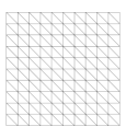
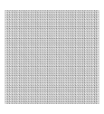
In this section, the results of several numerical examples are presented. All results are obtained on a square domain $\Omega=[x_{0},x_{0}+L]\times[y_{0},y_{0}+L]$ where we denote by $x_{0},y_{0}$ the origin of the $(x,y)$ coordinate system, and $L$ is the domain size in the x and y directions. A set of uniform triangular meshes is used to discretize the computational domain $\Omega$ as shown in Figure 1. In all simulations, we set $\beta_{0}=(k+1)^{2}$, $\beta_{0v}=\frac{\beta_{0}}{2}$ and $\beta_{1}=\frac{1}{2k(k+1)}$ in the numerical flux definitions, and the time integration is performed by a third order explicit strong stability-preserving (SSP) Runge-Kutta scheme [40]. Unless stated otherwise, the time step size $\Delta t$ is determined by the following Courant-Friedrichs-Levy (CFL) rule:

(25) $$\Delta t\frac{\mu}{\min_{K}{h^{2}_{K}}}<\omega\lambda,$$

where $\lambda$ is the CFL number, $\mu$ is a diffusion constant and $\omega$ is the minimum quadrature weight for the volume integration developed in [49].

Furthermore, the convergence rates are reported only in the $L_{2}$ and $L_{\infty}$ norms. To do that, we employ the $(k+1)th$ order quadrature rule to calculate the $L_{2}$-error while the $L_{\infty}$-errors are measured using $361$ points generated by the same quadrature rule in each element.

(a) $h$

(b) $h/2$

(c) $h/4$

(d) $h/8$

Figure 1: The set of uniform unstructured meshes with $h=L/5$

Example 5.1. In this example, we consider the heat equation

$$\frac{\partial U}{\partial t}=\mu\Delta U,$$

with periodic boundary conditions on $\Omega=[0,1]\times[0,1]$ where $\mu$ is a constant diffusion coefficient. Note that the diffusion matrix $A(u)$ is given as

$$A(u)=\mu\mathbb{I},$$

where $\mathbb{I}\in\mathbb{R}^{2\times 2}$ is the identity matrix. The initial condition for this example is obtained from the following exact solution at $t=0$:

$$U(x,y,t)=e^{-8\pi^{2}\mu t}\cos\left(2\pi(x+y)\right).$$

In this example, we set $\lambda=0.1$, $\mu=0.01$ and $T=1$. In addition, all quadrature rules are exact up to polynomials of degree $2k+1$.

The $L_{2}$ and $L_{\infty}$ errors are listed in Tables 1 and 2, respectively. We observe that optimal $(k+1)th$ order convergence in the $L_{2}$-norm is obtained by the DDGIC and symmetric DDG methods without any order loss for even degree polynomials. On the other hand, the nonsymmetric DDG method is optimally convergent only for $k=3$ in the $L_{2}$-norm. For even degree polynomials, the convergence rate of the nonsymmetric DDG method is degrading as the mesh is refined. However, in the $L_{\infty}$-norm, all DDG methods demonstrate $(k+1)th$ order optimal convergence.

Table 1: $L_{2}$ errors for Example 5.1 at $T=1$

3	$L_{2}$ errors and orders for the DDGIC method
	$h$	$h/2$	Order	$h/4$	Order	$h/8$	Order
$k=2$	2.47E-03	3.10E-04	3.00	3.88E-05	3.00	4.85E-06	3.00
$k=3$	1.87E-04	1.17E-05	4.00	7.29E-07	4.00	4.55E-08	4.00
$k=4$	1.16E-05	3.64E-07	5.00	1.14E-08	5.00	3.55E-10	5.00
2
2	$L_{2}$ errors and orders for the symmetric DDG method
	$h$	$h/2$	Order	$h/4$	Order	$h/8$	Order
$k=2$	2.82E-03	3.55E-04	2.99	4.45E-05	2.99	5.56E-06	3.00
$k=3$	2.10E-04	1.30E-05	4.01	8.10E-07	4.00	5.06E-08	4.00
$k=4$	1.28E-05	4.02E-07	4.99	1.26E-08	5.00	3.93E-10	5.00
2
2	$L_{2}$ errors and orders for the nonsymmetric DDG method
	$h$	$h/2$	Order	$h/4$	Order	$h/8$	Order
$k=2$	2.29E-03	2.88E-04	2.99	3.73E-05	2.95	5.20E-06	2.84
$k=3$	1.85E-04	1.15E-05	4.01	7.21E-07	4.00	4.50E-08	4.00
$k=4$	1.13E-05	3.66E-07	4.95	1.26E-08	4.86	5.12E-10	4.62
3

Table 2: $L_{\infty}$ errors for Example 5.1 at $T=1$

3	$L_{\infty}$ errors and orders for the DDGIC method
	$h$	$h/2$	Order	$h/4$	Order	$h/8$	Order
$k=2$	8.58E-03	1.03E-03	3.06	1.31E-04	2.97	1.65E-05	2.99
$k=3$	7.77E-04	5.40E-05	3.85	3.43E-06	3.98	2.17E-07	3.98
$k=4$	4.63E-05	1.35E-06	5.10	4.23E-08	4.99	1.32E-09	5.00
2
2	$L_{\infty}$ errors and orders for the symmetric DDG method
	$h$	$h/2$	Order	$h/4$	Order	$h/8$	Order
$k=2$	6.15E-03	7.01E-04	3.13	8.96E-05	2.97	1.13E-05	2.99
$k=3$	6.18E-04	4.36E-05	3.83	2.83E-06	3.94	1.79E-07	3.98
$k=4$	3.39E-05	1.01E-06	5.07	3.26E-08	4.96	1.03E-09	4.99
2
2	$L_{\infty}$ errors and orders for the nonsymmetric DDG method
	$h$	$h/2$	Order	$h/4$	Order	$h/8$	Order
$k=2$	1.14E-02	1.39E-03	3.03	1.83E-04	2.92	2.32E-05	2.98
$k=3$	9.58E-04	6.56E-05	3.87	4.10E-06	4.00	2.59E-07	3.98
$k=4$	6.04E-05	1.86E-06	5.02	6.08E-08	4.94	1.96E-09	4.96
3

Example 5.2. In this numerical test, we now consider an anisotropic diffusion equation with mixed derivatives

$$\frac{\partial U}{\partial t}=\mu\left(2U_{xx}+3U_{xy}+3U_{yy}\right),$$

with periodic boundary conditions on $\Omega=[0,1]\times[0,1]$. Note that this equation is still linear, i.e. diffusion matrix $A(u)$ is a constant coefficient matrix. Moreover, it can be written in a nonsymmetric form

$$A(u)=\mu\begin{pmatrix}2&1\\ 2&3\end{pmatrix}.$$

A nonsymmetric diffusion matrix is chosen to see how the new DDG methods would behave in such a setting. The initial condition is set from the following exact solution at $t=0$:

(26) $$U(x,y,t)=e^{-32\pi^{2}\mu t}\cos(2\pi y)\cos(4\pi x-2\pi y).$$

As in the previous example, we set $\lambda=0.1$, $\mu=0.01$, $T=1$, and all quadrature rules are exact up to polynomials of degree $2k+1$.

The $L_{2}$ and $L_{\infty}$ errors are listed in Tables 3 and 4, respectively. The DDGIC and symmetric DDG methods behave similarly in all cases. For the even degree polynomials, these methods do not lose order. On the other hand, the nonsymmetric DDG method demonstrates optimal $(k+1)$ convergence only for $k=3$ while it loses an order for even degree polynomials, which is clearer compared to Example 5.1. Furthermore, the order loss is not only seen in the $L_{2}$-error but also clearly observed in the $L_{\infty}$-error in this case.

Remark 5.1.

This problem has been also tested equivalently with the diffusion matrix

$$A(u)=\mu\begin{pmatrix}2&1.5\\ 1.5&3\end{pmatrix},$$

which is symmetric-positive definite. We note that the performance of the new DDG methods does not change with this diffusion matrix and the same results in Tables 3 and 4 are obtained. Therefore, those results are not reported.

Table 3: $L_{2}$ errors for Example 5.2 at $T=1$

3	$L_{2}$ errors and orders for the DDGIC method
	$h$	$h/2$	Order	$h/4$	Order	$h/8$	Order
$k=2$	1.34E-02	2.59E-03	2.37	2.14E-04	3.60	1.76E-05	3.61
$k=3$	3.37E-03	1.16E-04	4.87	5.31E-06	4.45	3.12E-07	4.09
$k=4$	4.62E-04	1.19E-05	5.29	3.73E-07	4.99	1.18E-08	4.99
2
2	$L_{2}$ errors and orders for the symmetric DDG method
	$h$	$h/2$	Order	$h/4$	Order	$h/8$	Order
$k=2$	1.41E-02	3.01E-03	2.22	2.56E-04	3.56	1.96E-05	3.71
$k=3$	3.68E-03	1.27E-04	4.86	5.51E-06	4.53	3.20E-07	4.11
$k=4$	4.92E-04	1.22E-05	5.33	3.88E-07	4.98	1.22E-08	4.99
2
2	$L_{2}$ errors and orders for the nonsymmetric DDG method
	$h$	$h/2$	Order	$h/4$	Order	$h/8$	Order
$k=2$	1.17E-02	2.47E-03	2.25	4.34E-04	2.51	9.21E-05	2.24
$k=3$	3.67E-03	2.00E-04	4.20	1.07E-05	4.23	6.35E-07	4.07
$k=4$	5.70E-04	1.15E-05	5.63	5.70E-07	4.34	3.47E-08	4.04
3

Table 4: $L_{\infty}$ errors for Example 5.2 at $T=1$

3	$L_{\infty}$ errors and orders for the DDGIC method
	$h$	$h/2$	Order	$h/4$	Order	$h/8$	Order
$k=2$	2.28E-02	4.33E-03	2.40	4.03E-04	3.43	4.04E-05	3.32
$k=3$	7.81E-03	3.68E-04	4.41	2.18E-05	4.08	1.41E-06	3.96
$k=4$	1.30E-03	3.48E-05	5.22	1.22E-06	4.84	3.97E-08	4.94
2
2	$L_{\infty}$ errors and orders for the symmetric DDG method
	$h$	$h/2$	Order	$h/4$	Order	$h/8$	Order
$k=2$	2.38E-02	4.96E-03	2.26	4.71E-04	3.40	4.54E-05	3.37
$k=3$	8.33E-03	4.03E-04	4.37	2.03E-05	4.31	1.28E-06	3.99
$k=4$	1.37E-03	3.61E-05	5.25	1.27E-06	4.82	4.17E-08	4.94
2
2	$L_{\infty}$ errors and orders for the nonsymmetric DDG method
	$h$	$h/2$	Order	$h/4$	Order	$h/8$	Order
$k=2$	2.13E-02	4.40E-03	2.28	8.01E-04	2.46	1.69E-04	2.25
$k=3$	8.39E-03	5.87E-04	3.84	4.10E-05	3.84	2.66E-06	3.95
$k=4$	1.49E-03	3.44E-05	5.43	1.50E-06	4.52	6.94E-08	4.44
3

Example 5.3. In this example, we consider the porous medium equation

(27) $$\frac{\partial U}{\partial t}=\mu\Delta(U^{\gamma}),$$

where $\gamma$ is a model parameter. Note that this equation models a nonlinear diffusion process for $\gamma\neq 1$, i.e. coefficients of the diffusion matrix $A(u)$ are functions of $u$:

$$A(u)=\mu\begin{pmatrix}\gamma u^{\gamma-1}&0\\ 0&\gamma u^{\gamma-1}\end{pmatrix}=\mu\gamma u^{\gamma-1}\mathbb{I},$$

where $\mathbb{I}\in\mathbb{R}^{2\times 2}$ is the identity matrix. Notice that the diffusion matrix is diagonal, but for $\gamma>1$, Equation 27 becomes highly nonlinear. In order to assess the performance of the new DDG methods in a highly nonlinear diffusion problem and measure the convergence rate, we solve Equation 27 on $\Omega=[0,1]\times[0,1]$ with $\gamma=3$ and employ the method of manufactured solutions by enforcing the solution

$$U(x,y,t)=e^{-8\pi^{2}\mu t}\sin(2\pi(x+y)).$$

The initial condition for this problem is obtained from this manufactured solution at $t=0$. Also, note that the boundary conditions are periodic. Furthermore, we set $\lambda=0.1$, $\mu=0.01$, $T=1$, and employ quadrature rules that are exact up to polynomials of degree $4k+1$.

The $L_{2}$ and $L_{\infty}$ errors are listed in Tables 5 and 6, respectively. We observe that all DDG methods converge with optimal $(k+1)th$ order accuracy for all reported cases. Although this problem is highly nonlinear, the optimal convergence might be due to the diagonal structure of the nonlinear diffusion matrix $A(u)$.

Table 5: $L_{2}$ errors for Example 5.3 at $T=1$

3	$L_{2}$ errors and orders for the DDGIC method
	$h$	$h/2$	Order	$h/4$	Order
$k=2$	3.19E-03	4.02E-04	2.99	5.00E-05	3.01
$k=3$	2.46E-04	1.29E-05	4.26	7.48E-07	4.10
$k=4$	1.74E-05	5.63E-07	4.95	1.54E-08	5.20
2
2	$L_{2}$ errors and orders for the symmetric DDG method
	$h$	$h/2$	Order	$h/4$	Order
$k=2$	3.26E-03	4.37E-04	2.90	5.64E-05	2.95
$k=3$	2.87E-04	1.43E-05	4.33	8.33E-07	4.10
$k=4$	1.85E-05	6.12E-07	4.91	1.69E-08	5.18
2
2	$L_{2}$ errors and orders for the nonsymmetric DDG method
	$h$	$h/2$	Order	$h/4$	Order
$k=2$	2.93E-03	4.41E-04	2.73	5.19E-05	3.09
$k=3$	2.09E-04	1.31E-05	3.99	8.54E-07	3.94
$k=4$	1.72E-05	5.23E-07	5.04	1.50E-08	5.13
3

Table 6: $L_{\infty}$ errors for Example 5.3 at $T=1$

3	$L_{\infty}$ errors and orders for the DDGIC method
	$h$	$h/2$	Order	$h/4$	Order
$k=2$	2.42E-02	3.87E-03	2.65	5.33E-04	2.86
$k=3$	2.29E-03	7.78E-05	4.88	3.45E-06	4.49
$k=4$	2.60E-04	1.06E-05	4.62	3.50E-07	4.92
2
2	$L_{\infty}$ errors and orders for the symmetric DDG method
	$h$	$h/2$	Order	$h/4$	Order
$k=2$	2.29E-02	3.54E-03	2.69	4.97E-04	2.83
$k=3$	2.05E-03	5.61E-05	5.19	2.78E-06	4.33
$k=4$	2.45E-04	1.02E-05	4.59	3.41E-07	4.90
2
2	$L_{\infty}$ errors and orders for the nonsymmetric DDG method
	$h$	$h/2$	Order	$h/4$	Order
$k=2$	2.69E-02	4.46E-03	2.59	6.06E-04	2.88
$k=3$	2.45E-03	6.97E-05	5.14	4.32E-06	4.01
$k=4$	2.79E-04	1.15E-05	4.61	3.70E-07	4.95
3

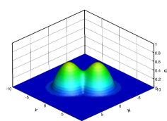
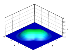
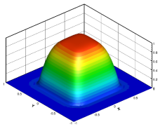
Example 5.4. In this example, we consider the same equation as in Example 5.3, but with the model coefficient $\gamma=2$ on $\Omega=[-10,10]\times[-10,10]$. Here, we investigate the performance of the new DDG methods for two initially disconnected, merging bumps which are defined by the following:

$$U_{0}(x,y)=\begin{cases}e^{\frac{-1}{6-(x-2)^{2}-(y+2)^{2}}},&(x-2)^{2}-(y+2)^{2}<6\\ e^{\frac{-1}{6-(x+2)^{2}-(y-2)^{2}}},&(x+2)^{2}-(y-2)^{2}<6\\ 0,&\text{otherwise}.\end{cases}$$

Note that $U(x,y,t)=0$ on $\partial\Omega$ for $t\geq 0$. In this case, we solve the problem on $h/16$ mesh along with $\lambda=0.1$, $\mu=1$ and $T=4$. In Figure 2, we present a third order ($k=2$) symmetric DDG solution. The solutions corresponding to other DDG versions are similar, hence they are not included. In this case, we solve the problem on $h/16$ mesh along with $\lambda=0.1$, $\mu=1$ and $T=4$. We observe that bumps are diffused quickly and merged with finite time. The results are in good agreement with those in literature [41, 43, 33]

(a) $t=0$

(b) $t=0.5$

(c) $t=1$

(d) $t=4$

Figure 2: The contour plot corresponding to the third ($k=2$) order symmetric DDG solution for Example 5.4. 17 equally spaced contours are used between $0$ and $0.8$.

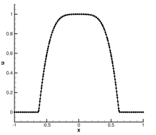
Example 5.5 In this example, we continue to study the same equation as in Example 5.3, but with the model coefficient $\gamma=2$ on $\Omega=[-1,1]\times[-1,1]$. $U(x,y,t)=0$ on $\partial\Omega$ for $t\geq 0$ and the initial condition is defined as

$$U_{0}(x,y)=\begin{cases}1,&(x,y)\in[-\frac{1}{2},\frac{1}{2}]\times[-\frac{1}{2},\frac{1}{2}]\\ 0,&\text{otherwise}.\end{cases}$$

We set $\lambda=0.1$, $\mu=1$ and $T=0.005$ and solve the problem on $h/16$ mesh.

Since the initial condition is discontinuous, the numerical solutions obtained by the new DDG methods blow up unless a maximum-principle-satisfying (MPS) limiter is employed. Therefore, the linear scaling limiter in [47] is implemented to keep the numerical solution in $0\leq u(x,y,t)\leq 1$ for $t\geq 0$. Note that the CFL condition Equation 25 is still in use, and the DDG parameters $\beta_{0}$ and $\beta_{1}$ are kept the same.

In Figure 3, the numerical solution obtained by the DDGIC method for a third order numerical solution ($k=2$) is shown. We observe that the numerical solution diffuses out smoothly in a stable manner and is in good agreement with Example 5.7 of [23].

(a)

(b)

Figure 3: The third ($k=2$) order numerical solution obtained by DDGIC with MPS limiter for Example 5.4 at $T=0.005$. (a) The solution along $y=0$, (b) surface plot. 19 equally spaced contour levels are used between 0 and 1.

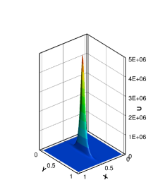
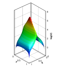
Example 5.6 In this example, we consider

(28) $$\frac{\partial U}{\partial t}=\mu\left(2U_{xx}+3(U^{1.5})_{yy}+U^{2}\right),$$

with the initial condition $U_{0}(x,y)=200\sin{(\pi x)}\sin{(\pi y)}$ on $\Omega=[0,1]\times[0,1]$. We apply the homogeneous Dirichlet boundary condition. Due to the last term on the right-hand side of Equation 28, the solution eventually blows up. As reported in Example 3.7 of [25], we observe that the numerical solution blows up after one time-step when a positivity-preserving limiter is not used. Therefore, the linear scaling limiter in [47] is employed to maintain the stability of the numerical approximation. However, the limiter’s upper bound condition on the numerical solution is removed and the lower bound is set to 0 to preserve the positivity of the numerical solution. Furthermore, according to [25], the CFL condition in Equation 25 is modified as

$$\Delta t\frac{\mu}{\min_{K}{h^{2}_{K}}}<\min{\left(\omega\lambda,\frac{1}{\max_{K}{u}}\right)}.$$

As in the previous example, the DDG parameters $\beta_{0},\beta_{1}$ are kept the same. The $h/16$ mesh is used to solve this problem, and we set $\lambda=0.01$, $\mu=1$, and the quadrature rules are exact up to polynomials of degree $(2k+1)th$. As for the stopping criterion, we follow [25] and take $\Delta t<10^{-13}$. However, it is worth emphasizing that the focus of this paper is not to design a positivity-preserving limiter. Instead, we simply explore the performance of the new DDG methods in computationally challenging cases. Therefore, the modified CFL condition along with the linear scaling limiter does not guarantee the positivity of the numerical solution for the time level $t^{n+1}$. In fact, almost all of the MPS or positivity-preserving limiters are designed for forward Euler method, but instead, they are used in a Runge-Kutta scheme. Even though they might propose a CFL condition that might guarantee the positivity (or maximum-principle) of the numerical solution for a forward Euler method, the physical limits of the problem might be violated by the numerical solution at any stage of the Runge-Kutta scheme. Therefore, we follow [46] and restart the Runge-Kutta time step with $\Delta t/2$ when it is no longer possible to maintain the positivity of the numerical solution in one or more cells.

For a third ($k=2$) order solution, we observe that the restart algorithm is only activated at the last time-step at $t=1.8155\times 10^{-2}$ for all DDG versions. However, it turns out that the time step becomes smaller than the machine precision $\epsilon$, i.e. $\Delta t<\epsilon$, during the restart procedure. This means that it is no longer possible to continue time-stepping without violating the positivity in one or more cells. Therefore, we denote $t=1.81552\times 10^{-2}$ as the blow-up time. Note that this value is slightly smaller than the blow-up time $t=1.82378\times 10^{-2}$ reported in [25]. Thus, we obtain slightly lower values for $\max_{K}{u_{K}}$. In Figure 4, we show the numerical solution for a third order ($k=2$) numerical solution obtained by the DDGIC method when the solution blows up at $t=1.81552\times 10^{-2}$. Since the results obtained by other DDG versions are similar, they are not shown. We observe that the numerical solution does not have oscillations and qualitatively similar to that in [25].

(a) u

(b) log(u)

Figure 4: The third ($k=2$) order numerical solution obtained by DDGIC with MPS limiter for Example 5.6 at $T=1.81552\times 10^{-2}$

6 Concluding Remarks

In this paper, we have unified the new framework for direct discontinuous Galerkin (DDG) methods by extending the new DDGIC method [22] to the symmetric and the nonsymmetric DDG versions. Unlike their original counterparts, the new DDG methods do not require evaluating an antiderivative of the nonlinear diffusion matrix. By constructing a new direction vector at each element interface, a linear numerical flux is used regardless of the problem type. Furthermore, the nonlinear linear stability theory of the new methods has been developed and several numerical experiments have been conducted to perform the error analysis. In all numerical examples, the DDGIC and symmetric DDG methods demonstrated optimal $(k+1)th$ order convergence and their performances were assessed to be equivalent. On the other hand, the performance of the nonsymmetric DDG method varied in all numerical examples. The nonsymmetric DDG method achieved optimal $(k+1)th$ order convergence for odd degree polynomials in all examples while an order loss was observed with the even degree polynomials except for the cases with diagonal diffusion matrices. In short, a high-order accuracy is achieved by all new DDG methods. However, the DDGIC and symmetric DDG methods were found to be superior to the nonsymmetric version.

Appendix A Important Inequalities

In this section, we discuss important inequalities used in the proofs of the stability analysis for symmetric DDG and DDGIC methods.

Lemma A.1 (Young’s inequality).

Suppose that $a,b\geq 0$, $1<p,q,\infty$, and that $\frac{1}{p}+\frac{1}{q}=1$. Then, we have that

$$ab\leq\frac{a^{p}}{p}+\frac{b^{q}}{q}.$$

A corollary to Lemma A.1 can be obtained by considering $ab=(a\epsilon^{1/p})(b/\epsilon^{1/p})$ for $\epsilon>0$.

Corollary A.2.

Suppose that $a,b\geq 0$, $1<p,q,\infty$, and that $\frac{1}{p}+\frac{1}{q}=1$. Furthermore, if $\epsilon>0$, then

$$ab\leq\frac{\epsilon a^{p}}{p}+\frac{b^{q}}{q\epsilon^{q/p}}.$$

We will also recall the following lemma due to Ern and Guermord [24]:

Lemma A.3.

Let $v\in\mathbb{V}_{h}^{k}$ and $l\in\mathbb{N}$. There exists a constant $C>0$ for any non-negative integer $m\leq l$ such that

$$\left|v\right|_{W^{l,p}(K)}\leq Ch_{K}^{m-l+d\left(\frac{1}{p}-\frac{1}{r}\right)}\left|v\right|_{W^{m,r}(K)},\quad\forall p,r\in[1,\infty].$$

Proof A.4.

See the proof of Lemma 12.1 in [24].

Next, we will derive a series of essential inequalities used in the proof of the stability results for symmetric DDG and DDGIC methods.

Lemma A.5.

Assume that $A(u)\in\mathbb{R}^{2\times 2}$ is positive definite and there exist $\gamma,\gamma^{*}\in\mathbb{R}$ such that the eigenvalues $(\gamma_{1},\gamma_{2})$ of $A(u)$ lie between $[\gamma,\gamma^{*}]$ for $\forall u\in\mathbb{R}$. If $\boldsymbol{\xi}(u)$ is given as in Equation 7, then $\forall\mathbf{x}\in\mathbb{R}^{2}$ there holds

$$\left|\boldsymbol{\xi}(u)\cdot\mathbf{x}\right|\leq\gamma^{*}\left\|\mathbf{x}\right\|,$$

where we denote by $\left\|\cdot\right\|$ the Euclidean norm in $\mathbb{R}^{2}$.

Proof A.6.

Using the Scharwz inequality, we have

$$\left|\boldsymbol{\xi}(u)\cdot\mathbf{x}\right|\leq\left\|\boldsymbol{\xi}(u)\right\|\left\|\mathbf{x}\right\|.$$

Let $\mathbf{e}_{1},\mathbf{e}_{2}$ be the orthonormal eigenvectors corresponding to the eigenvalues $\gamma\text{ and }\gamma^{*}$, respectively. Since $A(u)$ is positive-definite, its eigenvectors form a basis of $\mathbb{R}^{2}$. Then, the unit normal vector can be written as $\mathbf{n}=n_{1}\mathbf{e}_{1}+n_{2}\mathbf{e}_{2}$, and then, it follows that

$$\left\|\boldsymbol{\xi}(u)\right\|^{2} =\left\|A(\{\!\!\{u\}\!\!\})^{T}\mathbf{n}\right\|^{2}=\left\|\gamma_{1}n_{1}\mathbf{e}_{1}+\gamma_{2}n_{2}\mathbf{e}_{2}\right\|^{2}=\gamma_{1}^{2}n_{1}^{2}+\gamma_{2}^{2}n_{2}^{2}$$

$$\leq(\gamma^{*})^{2}\left(n_{1}^{2}+n_{2}^{2}\right)=(\gamma^{*})^{2}$$

and the conclusion holds.

Lemma A.7.

Suppose that $A(u)\in\mathbb{R}^{2\times 2}$ is positive definite and there exist $\gamma,\gamma^{*}\in\mathbb{R}$ such that the eigenvalues $(\gamma_{1},\gamma_{2})$ of $A(u)$ lie between $[\gamma,\gamma^{*}]$ for $\forall u\in\mathbb{R}$. If $\beta_{0}\geq 0$, then we have that

$$\sum_{e\in\mathcal{E}_{h}}\int_{e}\frac{\beta_{0}}{h_{e}}\llbracket u\rrbracket^{2}\mathbf{n}\cdot\boldsymbol{\xi}(\{\!\!\{u\}\!\!\})~{}ds\geq\sum_{e\in\mathcal{E}_{h}}\int_{e}\frac{\gamma\beta_{0}}{h_{e}}\llbracket u\rrbracket^{2}~{}ds.$$

Proof A.8.

Recall the definition of the new direction vector $\boldsymbol{\xi}\{\!\!\{u\}\!\!\}=A(\{\!\!\{u\}\!\!\})^{T}\mathbf{n}$. Then,

$$\frac{\beta_{0}}{h_{e}}\llbracket u\rrbracket^{2}\mathbf{n}\cdot\boldsymbol{\xi}(\{\!\!\{u\}\!\!\})=\frac{\beta_{0}}{h_{e}}\llbracket u\rrbracket^{2}\mathbf{n}\cdot A(\{\!\!\{u\}\!\!\})^{T}\mathbf{n}.$$

Since $\mathbf{n}\cdot A(\{\!\!\{u\}\!\!\})^{T}\mathbf{n}\geq\gamma_{1}\geq\gamma$, the conclusion follows.

Lemma A.9.

Suppose that $A(u)\in\mathbb{R}^{2\times 2}$ is positive definite and there exist $\gamma,\gamma^{*}\in\mathbb{R}$ such that the eigenvalues $(\gamma_{1},\gamma_{2})$ of $A(u)$ lie between $[\gamma,\gamma^{*}]$ for $\forall u\in\mathbb{V}_{h}^{k}$. If $\beta_{0}\geq 0$, then there exists a constant $C>0$ such that

$$\sum_{e\in\mathcal{E}_{h}}\int_{e}\llbracket u\rrbracket\{\!\!\{\nabla u\}\!\!\}\cdot\boldsymbol{\xi}(\{\!\!\{u\}\!\!\})~{}ds\geq-\sum_{e\in\mathcal{E}_{h}}\frac{\gamma\beta_{0}}{2h}\left\|\llbracket u\rrbracket\right\|^{2}_{L^{2}(e)}-\sum_{K\in\mathcal{T}_{h}}C\frac{(\gamma^{*}k)^{2}}{4\gamma\beta_{0}}\left\|\nabla u\right\|^{2}_{L^{2}(K)}.$$

Furthermore, under the same assumptions, there also holds

$$\sum_{e\in\mathcal{E}_{h}}\int_{e}\llbracket u\rrbracket\{\!\!\{\nabla u\}\!\!\}\cdot\boldsymbol{\xi}(\{\!\!\{u\}\!\!\})~{}ds\geq-\sum_{e\in\mathcal{E}_{h}}\frac{\gamma\beta_{0}}{4h}\left\|\llbracket u\rrbracket\right\|^{2}_{L^{2}(e)}-\sum_{K\in\mathcal{T}_{h}}C\frac{(\gamma^{*}k)^{2}}{2\gamma\beta_{0}}\left\|\nabla u\right\|^{2}_{L^{2}(K)}.$$

Proof A.10.

Note that $\{\!\!\{\nabla u\}\!\!\}=\frac{1}{2}(\nabla u)^{+}+\frac{1}{2}(\nabla u)^{-}$. Then, we have

$$\sum_{e\in\mathcal{E}_{h}}\int_{e}\llbracket u\rrbracket\{\!\!\{\nabla u\}\!\!\} \cdot\boldsymbol{\xi}(\{\!\!\{u\}\!\!\})~{}ds$$

$$=\frac{1}{2}\sum_{e\in\mathcal{E}_{h}}\int_{e}\llbracket u\rrbracket\left((\nabla u)^{+}+(\nabla u)^{-}\right)\cdot\boldsymbol{\xi}(\{\!\!\{u\}\!\!\})~{}ds$$

$$\geq-\frac{1}{2}\sum_{e\in\mathcal{E}_{h}}\int_{e}\left|\llbracket u\rrbracket\right|\left(\left|(\nabla u)^{+}\cdot\boldsymbol{\xi}(\{\!\!\{u\}\!\!\})\right|+\left|(\nabla u)^{-}\cdot\boldsymbol{\xi}(\{\!\!\{u\}\!\!\})\right|\right)~{}ds$$

$$\geq-\frac{\gamma^{*}}{2}\sum_{e\in\mathcal{E}_{h}}\int_{e}\left|\llbracket u\rrbracket\right|\left\|(\nabla u)^{+}\right\|~{}ds-\frac{\gamma^{*}}{2}\sum_{e\in\mathcal{E}_{h}}\int_{e}\left|\llbracket u\rrbracket\right|\left\|(\nabla u)^{-}\right\|~{}ds,$$

where we have invoked Lemma A.5 in the last step. Moreover, by Corollary A.2 with $\epsilon=\frac{\gamma\beta_{0}}{\gamma^{*}h}$, we obtain

(29) $$\gamma^{*}\int_{e}\left|\llbracket u\rrbracket\right|\,\left\|(\nabla u)^{\pm}\right\|~{}ds\leq\frac{\gamma\beta_{0}}{2h}\left\|\llbracket u\rrbracket\right\|^{2}_{L^{2}(e)}+\frac{(\gamma^{*})^{2}h}{2\gamma\beta_{0}}\left\|(\nabla u)^{\pm}\right\|^{2}_{L^{2}(e)}.$$

So that we have

(30) $$\sum_{e\in\mathcal{E}_{h}}\int_{e}\llbracket u\rrbracket\{\!\!\{\nabla u\}\!\!\} \cdot\boldsymbol{\xi}(\{\!\!\{u\}\!\!\})~{}ds$$

$$\geq-\sum_{e\in\mathcal{E}_{h}}\frac{\gamma\beta_{0}}{2h}\left\|\llbracket u\rrbracket\right\|^{2}_{L^{2}(e)}$$

$$-\sum_{e\in\mathcal{E}_{h}}\frac{(\gamma^{*})^{2}h}{4\gamma\beta_{0}}\left\|(\nabla u)^{+}\right\|^{2}_{L^{2}(e)}-\sum_{e\in\mathcal{E}_{h}}\frac{(\gamma^{*})^{2}h}{4\gamma\beta_{0}}\left\|(\nabla u)^{-}\right\|^{2}_{L^{2}(e)}.$$

Note that the last two terms above are simply summations over individual edges in the triangulation $\mathcal{T}_{h}$, and each summation is responsible for accumulating $\left\|(\nabla u)^{\pm}\right\|^{2}_{L^{2}(e)}$ only from one side of the edge. In the global sense, these summations accumulate $\left\|(\nabla u)^{interior}\right\|^{2}_{L^{2}(\partial K)}$ for each cell $K$ in the domain. Thus, they can be converted into a single summation over cells. That is,

(31) $$\sum_{e\in\mathcal{E}_{h}}\frac{(\gamma^{*})^{2}h}{4\gamma\beta_{0}}\left\|(\nabla u)^{+}\right\|^{2}_{L^{2}(e)}+\sum_{e\in\mathcal{E}_{h}}\frac{(\gamma^{*})^{2}h}{4\gamma\beta_{0}}\left\|(\nabla u)^{-}\right\|^{2}_{L^{2}(e)}=\sum_{K\in\mathcal{T}_{h}}\frac{(\gamma^{*})^{2}h}{4\gamma\beta_{0}}\left\|\nabla u\right\|^{2}_{L^{2}(\partial K)}.$$

This expression is useful since we can invoke the trace inequality

(32) $$\sum_{K\in\mathcal{T}_{h}}\frac{(\gamma^{*})^{2}h}{4\gamma\beta_{0}}\left\|\nabla u\right\|^{2}_{L^{2}(\partial K)}\leq\sum_{K\in\mathcal{T}_{h}}C\frac{(\gamma^{*}k)^{2}}{4\gamma\beta_{0}}\left\|\nabla u\right\|^{2}_{L^{2}(K)},$$

for some constant $C>0$. Thus, substituting Equations 31 and 32 into Equation 30 completes the first part of the proof. The second part follows after following the same steps but using $\epsilon=\frac{\gamma\beta_{0}}{2\gamma^{*}h}$ in Equation 29 instead.

Lemma A.11.

Suppose that $A(u)\in\mathbb{R}^{2\times 2}$ is positive definite and there exist $\gamma,\gamma^{*}\in\mathbb{R}$ such that the eigenvalues $(\gamma_{1},\gamma_{2})$ of $A(u)$ lie between $[\gamma,\gamma^{*}]$ for $\forall u\in\mathbb{V}_{h}^{k}$. If $\beta_{0}\geq 0$, then there exists a constant $C>0$ such that

$$\sum_{e\in\mathcal{E}_{h}}\int_{e}\beta_{1}h\llbracket u\rrbracket\llbracket\nabla(\nabla u\cdot\mathbf{n})\rrbracket \cdot\boldsymbol{\xi}(\{\!\!\{u\}\!\!\})~{}ds$$

$$\geq-\sum_{e\in\mathcal{E}_{h}}\frac{\gamma\beta_{0}}{2h}\left\|\llbracket u\rrbracket\right\|^{2}_{L^{2}(e)}-\sum_{K\in\mathcal{T}_{h}}C\frac{(\gamma^{*}\beta_{1}k)^{2}}{\gamma\beta_{0}}\left\|\nabla u\right\|^{2}_{L^{2}(K)}.$$

Proof A.12.

By convention, the outward unit normal vector $\mathbf{n}$ is understood as $\mathbf{n}=\mathbf{n}^{+}$. Also, it can be understood in terms of the inward unit normal vector as $\mathbf{n}=-\mathbf{n}^{-}$. Therefore, the jump term for the second derivatives can be rewritten as

$$\llbracket\nabla(\nabla u\cdot\mathbf{n})\rrbracket=\left(\nabla(\nabla u\cdot\mathbf{n})\right)^{+}+\left(\nabla(\nabla u\cdot\mathbf{n})\right)^{-}.$$

With this understanding, we have that

$$\int_{e}\beta_{1}h\llbracket u\rrbracket\llbracket\nabla(\nabla u\cdot\mathbf{n})\rrbracket \cdot\boldsymbol{\xi}(\{\!\!\{u\}\!\!\})~{}ds$$

$$=\int_{e}\beta_{1}h\llbracket u\rrbracket\left((\nabla(\nabla u\cdot\mathbf{n}))^{+}+(\nabla(\nabla u\cdot\mathbf{n}))^{-}\right)\cdot\boldsymbol{\xi}(\{\!\!\{u\}\!\!\})~{}ds$$

$$\geq-\int_{e}\beta_{1}h\left|\llbracket u\rrbracket\right|\left|\left((\nabla(\nabla u\cdot\mathbf{n}))^{+}+(\nabla(\nabla u\cdot\mathbf{n}))^{-}\right)\cdot\boldsymbol{\xi}(\{\!\!\{u\}\!\!\})\right|~{}ds$$

$$\geq-\gamma^{*}\int_{e}\beta_{1}h\left|\llbracket u\rrbracket\right|\left(\left\|(\nabla(\nabla u\cdot\mathbf{n}))^{+}\right\|+\left\|(\nabla(\nabla u\cdot\mathbf{n}))^{-}\right\|\right)~{}ds.$$

Note that we have invoked Lemma A.5 and triangle inequality in the last step. Furthermore, by Corollary A.2 with $\epsilon=\frac{\gamma\beta_{0}}{2\gamma^{*}\beta_{1}h^{2}}$, we obtain

$$\gamma^{*}\int_{e}\beta_{1}h\left|\llbracket u\rrbracket\right|\left\|(\nabla(\nabla u\cdot\mathbf{n}))^{\pm}\right\|ds\leq\frac{\gamma\beta_{0}}{4h}\left\|\llbracket u\rrbracket\right\|^{2}_{L^{2}(e)}+\frac{(\gamma^{*}\beta_{1})^{2}h^{3}}{\gamma\beta_{0}}\left\|(\nabla(\nabla u\cdot\mathbf{n}))^{\pm}\right\|^{2}_{L^{2}(e)}.$$

Thus,

(33) $$\sum_{e\in\mathcal{E}_{h}}\int_{e}\beta_{1}h\llbracket u\rrbracket\llbracket\nabla(\nabla u\cdot\mathbf{n})\rrbracket\cdot\boldsymbol{\xi}(\{\!\!\{u\}\!\!\})~{}ds \geq-\sum_{e\in\mathcal{E}_{h}}\frac{\gamma\beta_{0}}{2h}\left\|\llbracket u\rrbracket\right\|^{2}_{L^{2}(e)}$$

$$-\sum_{e\in\mathcal{E}_{h}}\frac{(\gamma^{*}\beta_{1})^{2}h^{3}}{\gamma\beta_{0}}\left\|(\nabla(\nabla u\cdot\mathbf{n}))^{+}\right\|^{2}_{L^{2}(e)}$$

$$-\sum_{e\in\mathcal{E}_{h}}\frac{(\gamma^{*}\beta_{1})^{2}h^{3}}{\gamma\beta_{0}}\left\|(\nabla(\nabla u\cdot\mathbf{n}))^{-}\right\|^{2}_{L^{2}(e)}.$$

As in the proof of Lemma A.9, we convert the summations over edges to a summation over cells:

(34) $$\sum_{e\in\mathcal{E}_{h}}\frac{(\gamma^{*}\beta_{1})^{2}h^{3}}{\gamma\beta_{0}}\left\|(\nabla(\nabla u\cdot\mathbf{n}))^{+}\right\|^{2}_{L^{2}(e)} +\sum_{e\in\mathcal{E}_{h}}\frac{(\gamma^{*}\beta_{1})^{2}h^{3}}{\gamma\beta_{0}}\left\|(\nabla(\nabla u\cdot\mathbf{n}))^{-}\right\|^{2}_{L^{2}(e)}$$

$$=\sum_{K\in\mathcal{T}_{h}}\frac{(\gamma^{*}\beta_{1})^{2}h^{3}}{\gamma\beta_{0}}\left\|\nabla(\nabla u\cdot\mathbf{n})\right\|^{2}_{L^{2}(\partial K)}.$$

At this point, it might be tempting to invoke the trace theorem for the norm on the right-hand side of the above equation. However, a more useful inequality can be obtained by considering the Euclidean norm $\left\|\nabla(\nabla u\cdot\mathbf{n})\right\|^{2}$. We first note that

$$\left\|\nabla(\nabla u\cdot\mathbf{n})\right\|^{2} =(u_{xx}n_{1}+u_{yx}n_{2})^{2}+(u_{xy}n_{1}+u_{yy}n_{2})^{2}$$

$$=(u_{xx}^{2}+u_{xy}^{2})n_{1}^{2}+(u_{yx}^{2}+u_{yy}^{2})n_{2}^{2}+2n_{1}n_{2}(u_{xx}u_{yx}+u_{xy}u_{yy}).$$

For the cross-product term above, we invoke Lemma A.1 with $p=q=2$

$$2n_{1}n_{2}(u_{xx}u_{yx}+u_{xy}u_{yy}) =2\left((n_{2}u_{xx})(n_{1}u_{yx})+(n_{2}u_{xy})(n_{1}u_{yy})\right)$$

$$\leq(u_{xx}^{2}+u_{xy}^{2})n_{2}^{2}+(u_{yx}^{2}+u_{yy}^{2})n_{1}^{2}.$$

Since $n_{1}^{2}+n_{2}^{2}=1$, we obtain

$$\left\|\nabla(\nabla u\cdot\mathbf{n})\right\|^{2}\leq u_{xx}^{2}+u_{xy}^{2}+u_{yx}^{2}+u_{yy}^{2}.$$

Using this and the trace inequality gives

$$\left\|\nabla(\nabla u\cdot\mathbf{n})\right\|^{2}_{L^{2}(\partial K)} =\int_{\partial K}\left\|\nabla(\nabla u\cdot\mathbf{n})\right\|^{2}~{}ds$$

$$\leq\int_{\partial K}\left(u_{xx}^{2}+u_{xy}^{2}+u_{yx}^{2}+u_{yy}^{2}\right)~{}ds$$

$$\leq C\frac{k^{2}}{h}\int_{K}\left(u_{xx}^{2}+u_{xy}^{2}+u_{yx}^{2}+u_{yy}^{2}\right)~{}dxdy=C\frac{k^{2}}{h}\left|u\right|^{2}_{H^{2}(K)}.$$

By Lemma A.3 with $d=l=p=r=2$ and $m=1$, we have

$$\left|u\right|_{H^{2}(K)}\leq\frac{C}{h}\left|u\right|_{H^{1}(K)}=\frac{C}{h}\left\|\nabla u\right\|_{L^{2}(K)},$$

which leads to

(35) $$\left\|\nabla(\nabla u\cdot\mathbf{n})\right\|^{2}_{L^{2}(\partial K)}\leq C\frac{k^{2}}{h^{3}}\left\|\nabla u\right\|^{2}_{L^{2}(K)}.$$

Finally, substituting Equations 34 and 35 in Equation 33 leads to the desired result.

References

- [1] D. N. Arnold, An interior penalty finite element method with discontinuous elements, SIAM journal on numerical analysis, 19 (1982), pp. 742–760.
- [2] D. N. Arnold, F. Brezzi, B. Cockburn, and L. D. Marini, Unified analysis of discontinuous galerkin methods for elliptic problems, SIAM journal on numerical analysis, 39 (2002), pp. 1749–1779.
- [3] G. A. Baker, Finite element methods for elliptic equations using nonconforming elements, Mathematics of Computation, 31 (1977), pp. 45–59.
- [4] F. Bassi, A. Crivellini, S. Rebay, and M. Savini, Discontinuous galerkin solution of the reynolds-averaged navier–stokes and k– turbulence model equations, Computers & Fluids, 34 (2005), pp. 507–540.
- [5] F. Bassi and S. Rebay, A high-order accurate discontinuous finite element method for the numerical solution of the compressible navier–stokes equations, Journal of Computational Physics, 131 (1997), pp. 267–279.
- [6] F. Bassi and S. Rebay, Gmres discontinuous galerkin solution of the compressible navier-stokes equations, in Discontinuous Galerkin Methods, Springer, 2000, pp. 197–208.
- [7] F. Bassi and S. Rebay, A high order discontinuous galerkin method for compressible turbulent flows, in Discontinuous Galerkin Methods, Springer, 2000, pp. 77–88.
- [8] C. E. Baumann and J. T. Oden, A discontinuous hp finite element method for convection—diffusion problems, Computer Methods in Applied Mechanics and Engineering, 175 (1999), pp. 311–341.
- [9] C. E. Baumann and J. T. Oden, A discontinuous hp finite element method for the euler and navier–stokes equations, International Journal for Numerical Methods in Fluids, 31 (1999), pp. 79–95.
- [10] S. C. Brenner, L. Owens, and L.-Y. Sung, A weakly over-penalized symmetric interior penalty method, Electronic transactions on numerical analysis, 30 (2008), p. 107.
- [11] A. Chen, F. Li, and Y. Cheng, An ultra-weak discontinuous galerkin method for schrödinger equation in one dimension, Journal of scientific computing, 78 (2018), pp. 772–815.
- [12] Z. Chen, H. Huang, and J. Yan, Third order maximum-principle-satisfying direct discontinuous galerkin methods for time dependent convection diffusion equations on unstructured triangular meshes, Journal of Computational Physics, 308 (2016), pp. 198 – 217.
- [13] Y. Cheng and C.-W. Shu, A discontinuous galerkin finite element method for time dependent partial differential equations with higher order derivatives, Mathematics of computation, 77 (2008), pp. 699–730.
- [14] B. Cockburn and C. Dawson, Approximation of the velocity by coupling discontinuous galerkin and mixed finite element methods for flow problems, Computational Geosciences, 6 (2002), pp. 505–522.
- [15] B. Cockburn, J. Gopalakrishnan, and R. Lazarov, Unified hybridization of discontinuous galerkin, mixed, and continuous galerkin methods for second order elliptic problems, SIAM Journal on Numerical Analysis, 47 (2009), pp. 1319–1365, https://doi.org/10.1137/070706616, https://doi.org/10.1137/070706616, https://arxiv.org/abs/https://doi.org/10.1137/070706616.
- [16] B. Cockburn, S. Hou, and C.-W. Shu, The runge-kutta local projection discontinuous galerkin finite element method for conservation laws. iv. the multidimensional case, Mathematics of Computation, 54 (1990), pp. 545–581.
- [17] B. Cockburn, C. Johnson, C.-W. Shu, and E. Tadmor, Advanced numerical approximation of nonlinear hyperbolic equations, vol. 1697 of Lecture Notes in Mathematics, Springer-Verlag, Berlin, 1998.
- [18] B. Cockburn, S.-Y. Lin, and C.-W. Shu, Tvb runge-kutta local projection discontinuous galerkin finite element method for conservation laws iii: one-dimensional systems, Journal of Computational Physics, 84 (1989), pp. 90–113.
- [19] B. Cockburn and C.-W. Shu, Tvb runge-kutta local projection discontinuous galerkin finite element method for conservation laws. ii. general framework, Mathematics of computation, 52 (1989), pp. 411–435.
- [20] B. Cockburn and C.-W. Shu, The local discontinuous galerkin method for time-dependent convection-diffusion systems, SIAM Journal on Numerical Analysis, 35 (1998), pp. 2440–2463.
- [21] B. Cockburn and C.-W. Shu, The runge–kutta discontinuous galerkin method for conservation laws v: multidimensional systems, Journal of Computational Physics, 141 (1998), pp. 199–224.
- [22] M. E. Danis and J. Yan, A new direct discontinuous galerkin method with interface correction for two-dimensional compressible navier-stokes equations, arXiv preprint arXiv:2104.09767, (2021).
- [23] J. Du and Y. Yang, Maximum-principle-preserving third-order local discontinuous galerkin method for convection-diffusion equations on overlapping meshes, Journal of Computational Physics, 377 (2019), pp. 117–141, https://doi.org/https://doi.org/10.1016/j.jcp.2018.10.034, https://www.sciencedirect.com/science/article/pii/S0021999118307010.
- [24] A. Ern and J.-L. Guermond, Finite elements I: Approximation and interpolation, vol. 72, Springer Nature, 2021.
- [25] L. Guo and Y. Yang, Positivity preserving high-order local discontinuous galerkin method for parabolic equations with blow-up solutions, Journal of Computational Physics, 289 (2015), pp. 181–195, https://doi.org/https://doi.org/10.1016/j.jcp.2015.02.041, https://www.sciencedirect.com/science/article/pii/S0021999115001114.
- [26] R. Hartmann and P. Houston, Symmetric interior penalty dg methods for the compressible navier–stokes equations ii: Goal–oriented a posteriori error estimation, International Journal of Numerical Analysis & Modeling, 3 (2006), pp. 141–162.
- [27] R. Hartmann and P. Houston, Symmetric interior penalty dg methods for the compressible navier-stokes equations i: Method formulation, International Journal of Numerical Analysis & Modeling, 3 (2006), pp. 1–20.
- [28] R. Hartmann and P. Houston, An optimal order interior penalty discontinuous galerkin discretization of the compressible navier–stokes equations, Journal of Computational Physics, 227 (2008), pp. 9670–9685.
- [29] H. Huang, J. Li, and J. Yan, High order symmetric direct discontinuous Galerkin method for elliptic interface problems with fitted mesh, J. Comput. Phys., 409 (2020), pp. 109301, 23.
- [30] G. Lin, J. Liu, and F. Sadre-Marandi, A comparative study on the weak galerkin, discontinuous galerkin, and mixed finite element methods, Journal of Computational and Applied Mathematics, 273 (2015), pp. 346–362, https://doi.org/https://doi.org/10.1016/j.cam.2014.06.024, https://www.sciencedirect.com/science/article/pii/S0377042714003057.
- [31] H. Liu and J. Yan, The direct discontinuous galerkin (DDG) methods for diffusion problems, SIAM Journal on Numerical Analysis, 47 (2008), pp. 675–698.
- [32] H. Liu and J. Yan, The direct discontinuous galerkin (DDG) method for diffusion with interface corrections, Communications in Computational Physics, 8 (2010), p. 541.
- [33] Y. Liu, C.-W. Shu, and M. Zhang, High order finite difference weno schemes for nonlinear degenerate parabolic equations, SIAM Journal on Scientific Computing, 33 (2011), pp. 939–965.
- [34] C. Qiu, Q. Liu, and J. Yan, Third order positivity-preserving direct discontinuous Galerkin method for chemotaxis keller-segel equation, J. Comput. Phys., accepted (2020).
- [35] W. H. Reed and T. Hill, Triangular mesh methods for the neutron transport equation, tech. report, Los Alamos Scientific Lab., N. Mex.(USA), 1973.
- [36] B. Rivière, M. F. Wheeler, and V. Girault, Improved energy estimates for interior penalty, constrained and discontinuous galerkin methods for elliptic problems. part i, Computational Geosciences, 3 (1999), pp. 337–360.
- [37] B. Rivière, M. F. Wheeler, and V. Girault, A priori error estimates for finite element methods based on discontinuous approximation spaces for elliptic problems, SIAM Journal on Numerical Analysis, 39 (2001), pp. 902–931.
- [38] C.-W. Shu, Discontinuous Galerkin method for time-dependent problems: survey and recent developments, in Recent developments in discontinuous Galerkin finite element methods for partial differential equations, vol. 157 of IMA Vol. Math. Appl., Springer, 2014, pp. 25–62.
- [39] C.-W. Shu, Discontinuous galerkin methods for time-dependent convection dominated problems: Basics, recent developments and comparison with other methods, in Building Bridges: Connections and Challenges in Modern Approaches to Numerical Partial Differential Equations, Lecture Notes in Computational Science and Engineering, Springer International Publishing, Cham, 2016, pp. 371–399.
- [40] C.-W. Shu and S. Osher, Efficient implementation of essentially non-oscillatory shock-capturing schemes, Journal of Computational Physics, 77 (1988), pp. 439 – 471.
- [41] C. Vidden and J. Yan, A new direct discontinuous galerkin method with symmetric structure for nonlinear diffusion equations, Journal of Computational Mathematics, 31 (2013), pp. 638–662.
- [42] M. F. Wheeler, An elliptic collocation-finite element method with interior penalties, SIAM Journal on Numerical Analysis, 15 (1978), pp. 152–161.
- [43] J. Yan, A new nonsymmetric discontinuous galerkin method for time dependent convection diffusion equations, Journal of Scientific Computing, 54 (2013), pp. 663–683.
- [44] J. Yan and C.-W. Shu, A local discontinuous galerkin method for kdv type equations, SIAM Journal on Numerical Analysis, 40 (2002), pp. 769–791.
- [45] M. Zhang and J. Yan, Fourier type super convergence study on DDGIC and symmetric DDG methods, J. Sci. Comput., 73 (2017), pp. 1276–1289.
- [46] X. Zhang, On positivity-preserving high order discontinuous Galerkin schemes for compressible Navier-Stokes equations, J. Comput. Phys., 328 (2017), pp. 301–343.
- [47] X. Zhang and C.-W. Shu, On maximum-principle-satisfying high order schemes for scalar conservation laws, Journal of Computational Physics, 229 (2010), pp. 3091–3120, https://doi.org/https://doi.org/10.1016/j.jcp.2009.12.030, https://www.sciencedirect.com/science/article/pii/S0021999109007165.
- [48] X. Zhang and C.-W. Shu, Maximum-principle-satisfying and positivity-preserving high-order schemes for conservation laws: survey and new developments, Proceedings of the Royal Society A: Mathematical, Physical and Engineering Sciences, 467 (2011), pp. 2752–2776.
- [49] X. Zhang, X. Zhang, Y. Xia, Y. Xia, C.-W. Shu, and C.-W. Shu, Maximum-principle-satisfying and positivity-preserving high order discontinuous galerkin schemes for conservation laws on triangular meshes, Journal of scientific computing, 50 (2012), pp. 29–62.