IXPE Detection of Polarized X-rays from Magnetars and Photon Mode Conversion at QED Vacuum Resonance

Abstract

The recent observations of the anomalous X-ray pulsars 4U 0142+61 and 1RXS J170849.0-400910 by the Imaging X-ray Polarimetry Explorer (IXPE) opened up a new avenue to study magnetars, neutron stars endowed with superstrong magnetic fields ($B\gtrsim 10^{14}$ G). The detected polarized X-rays from 4U 0142+61 exhibit a 90^∘ linear polarization swing from low photon energies ($E\lesssim 4$ keV) to high energies ($E\gtrsim 5.5$ keV). We show that this swing can be explained by photon polarization mode conversion at the vacuum resonance in the magnetar atmosphere; the resonance arises from the combined effects of plasma-induced birefringence and QED-induced vacuum birefringence in strong magnetic fields. This explanation suggests that the atmosphere of 4U 0142 be composed of partially ionized heavy elements, and the surface magnetic field be comparable or less than $10^{14}$ G, consistent with the dipole field inferred from the measured spindown. It also implies that the spin axis of 4U 0142+61 is aligned with its velocity direction. The polarized X-rays from 1RXS J170849.0-400910 do not show such $90^{\circ}$ swing, consistent with magnetar atmospheric emission with $B\gtrsim 5\times 10^{14}$ G.

Significance Statement: The recent detections of polarized X-rays from magnetars have opened up a new avenue to study magnetars, neutron stars endowed with superstrong magnetic fields. The detected polarization signals are intriguing, and can be explained by a novel QED vacuum resonance effect – an effect that is analogous to MSW neutrino oscillation that operates in the Sun and similar level-crossing phenomena in other areas of sciences.

Introduction

Magnetars are neutron stars (NSs) whose energy outputs (even in quiescence) are dominated by magnetic field dissipations [Thompson & Duncan 1993, Kaspi & Beloborodov 2017]. Recently the NASA/ASI Imaging X-ray Polarimetry Explorer (IXPE) [Weisskopf et al. 2016] reported the detection of linearly polarized x-ray emission from the anomalous x-ray pulsar (AXP) 4U 0142+61, a magnetar with an inferred dipole magnetic field (based the spindown rate) of $\sim 10^{14}$ G [Taverna et al. 2022]. This is the first time that polarized x-rays have been detected from any astrophysical point sources. The overall phase-averaged linear polarization degree is $12\pm 1\%$ throughout the IXPE band (2-8 keV). Interestingly, there is a substantial variation of the polarization signal with energy: the polarization degree is $14\pm 1\%$ at 2-4 keV and $41\pm 7\%$ at 5.5-8 keV, while it drops below the detector sensitivity around 4-5 keV, where the polarization angle swings by $\sim 90^{\circ}$.

Taverna et al. [Taverna et al. 2022] considered several possibilities to explain the observed polarization swing, and suggested that the thermal x-rays from 4U 0142+61 are emitted from an extended region of the condensed neutron star (NS) surface. In this scenario, the 2-4 keV radiation is dominated by the O-mode (polarized in the plane spanned by the local magnetic field and the photon wave vector), while the 5.5-8 keV radiation by the X-mode (which is orthogonal to the O-mode) because of re-procession by resonant Compton scattering (RCS) in the magnetosphere.

While it is pre-mature to draw any firm conclusion without detailed modeling, the ”condensed surface + RCS” scenario may be problematic for several reasons: (i) At the surface temperature of $T_{s}\simeq 5\times 10^{6}$ K and $B_{14}\equiv B/(10^{14}\,{\rm G})\simeq 1$, as appropriate for 4U 0142, it is unlikely that the NS surface is in a condensed form, even if the surface composition is Fe [Medin & Lai 2007, Potekhin & Chabrier 2013], simply because the cohesive energy of the Fe solid is not sufficiently large [Medin & Lai 2006]. (ii) A stronger surface magnetic field is possible, but the emission from a condensed Fe surface (for typical magnetic field and photon emission directions at the surface) is dominated by the O-mode only for photon energies less than $E_{c}\simeq 0.1\eta Z^{2/5}B_{14}^{1/5}\,{\rm keV}$, where $\eta\lesssim 1$ [van Adelsberg et al. 2005, Potekhin et al. 2012]. An unrealistically strong field ($B_{14}\gtrsim 10^{5}$ for $Z=26$) would be required to make $E_{c}\gtrsim 4$ keV. (iii) As acknowledged by Taverna et al. (2022)[Taverna et al. 2022], the assumption that the phase-averaged low-energy photons are dominated by the O-mode would imply that the NS spin axis (projected in the sky plane) is orthogonal to the proper motion direction. This is in contradiction to the growing evidence of spin-kick alignment in pulsars [Lai et al. 2001, Johnston et al. 2005, Wang et al. 2006, Noutsos et al. 2013, Janka et al. 2022].

In this paper, we show that the 90^∘ linear polarization swing observed in 4U 0142 could be naturally explained by photon mode conversion associated the ”vacuum resonance” arising from QED and plasma birefringence in strong magnetic fields. The essential physics of this effect was already discussed in Ref. [Lai & Ho 2003a], where it was shown that for neutron stars with H atmospheres, thermal photons with $E\lesssim 1$ keV are polarized orthogonal to photons with $E\gtrsim 4$ keV, provided that the NS surface magnetic field is somewhat less than $10^{14}$ G. The purpose of this paper is to re-examine the mode conversion effect under more general conditions (particularly the atmosphere composition) and to present new semi-analytic calculations of the polarization signals for parameters relevant to 4U 0142. Most recently, IXPE detected polarized X-rays from another AXP 1RXS J170849.0-400910, and found that the polarization angle remains constant as a function of $E$ [Zane et al. 2023]. This result is expected for the magnetar atmospheric emission with $B\gtrsim 5\times 10^{14}$ G – we comment on this at the end of the paper.

Vacuum resonance and mode conversion

Quantum electrodynamics (QED) predicts that in a strong magnetic field the vacuum becomes birefringent [Heisenberg & Euler 1936, Schwinger 1951, Adler 1971, Tsai & Erber 1975, Heyl & Hernquist 1997]. This vacuum birefringence is significant for $B\gg B_{Q}=m_{e}^{2}c^{3}/(e\hbar)=4.414\times 10^{13}$ G, the critical QED field strength. However, when combined with the birefringence due to the magnetized plasma, vacuum polarization can greatly affect radiative transfer even when the field strength is modest. A “vacuum resonance” arises when the contributions from the plasma and vacuum polarization to the dielectric tensor “compensate” each other [Gnedin et al. 1978, Mészáros & Ventura 1979, Pavlov & Gnedin 1984, Lai & Ho 2022, Lai & Ho 2003a, Lai & Ho 2003b, Ho & Lai 2003].

Consider x-ray photons propagating in the magnetized NS atmospheric plasma. There are two polarization modes: the ordinary mode (O-mode) is mostly polarized parallel to the ${\bf k}$-${\bf B}$ plane, while the extraordinary mode (X-mode) is perpendicular to it, where ${\bf k}$ is the photon wave vector and ${\bf B}$ is the external magnetic field [Mészáros 1992]. Throughout the paper, we assume the photon energy $E$ satisfies $u_{e}=(E_{Be}/E)^{2}\gg 1$ and $E_{Bi}/E\ll 1$, where $E_{Be}=\hbar eB/(m_{e}c)=1158B_{14}$ keV and $E_{Bi}=0.63(Z/A)B_{14}$ keV are the electron and ion cyclotron energies, respectively. This distinction of photons modes is important since the two modes have very different absorption and scattering opacities in the atmosphere plasma (see below): while the O-mode opacities are similar to the zero-field values, the X-mode opacities are significantly reduced because the electric field of the photon (EM wave), being orthogonal to ${\bf B}$, cannot effectively perturb the motion of the electron in the plasma when $E\ll E_{Be}$. However, the above description of O-mode and X-mode breaks down near the “vacuum resonance”. To be concrete, let us set up the $xyz$ coordinates with ${\bf k}$ along the $z$-axis and ${\bf B}$ in the $x$-$z$ plane (such that $\hat{\bf B}\times\hat{\bf k}=\sin\theta_{\rm kB}\hat{\bf y}$, where $\theta_{\rm kB}$ is the angle between ${\bf k}$ and ${\bf B}$). We write the transverse ($xy$) electric field of the photon mode as ${\bf E}\propto(iK,1)$. The mode ellipticity $K$ is given by

$$K_{\pm}=\beta\pm\sqrt{\beta^{2}+1},$$ (1)

where

$$\beta\simeq{u_{e}^{1/2}\sin^{2}\theta_{\rm kB}\over 2\cos\theta_{\rm kB}}\left(1-{\rho_{V}\over\rho}\right).$$ (2)

For a photon of energy $E$, the vacuum resonance density is given by

$$\rho_{V}\simeq 0.964\,Y_{e}^{-1}B_{14}^{2}E_{1}^{2}f^{-2}\leavevmode\nobreak\ {\rm g\leavevmode\nobreak\ cm}^{-3}$$ (3)

where $Y_{e}=\langle Z/A\rangle$ is the electron fraction, $E_{1}=E/(1\leavevmode\nobreak\ {\rm keV})$, and $f=f(B)$ is a slowly varying function of $B$ and is of order unity ($f=1$ for $B\ll B_{Q}$, $f\simeq 0.991$ at $B_{14}=1$ and $f\rightarrow(B/5B_{Q})^{1/2}$ for $B\gg B_{Q}$; see [Potekhin et al. 2004] for a general fitting formula). For $\rho>\rho_{V}$ (where the plasma effect dominates the dielectric tensor) and $\rho<\rho_{V}$ (where vacuum polarization dominates), the photon modes (for typical $\theta_{\rm kB}\neq 0$) are almost linearly polarized; near $\rho=\rho_{V}$, however, the normal modes become circularly polarized as a result of the “cancellation” of the plasma and vacuum effects (see Fig. 1). The half-width of the vacuum resonance (defined by $|\beta|<1$) is

$$\epsilon\equiv{\Delta\rho\over\rho_{V}}={2\cos\theta_{\rm kB}\over u_{e}^{1/2}\sin^{2}\theta_{\rm kB}}.$$ (4)

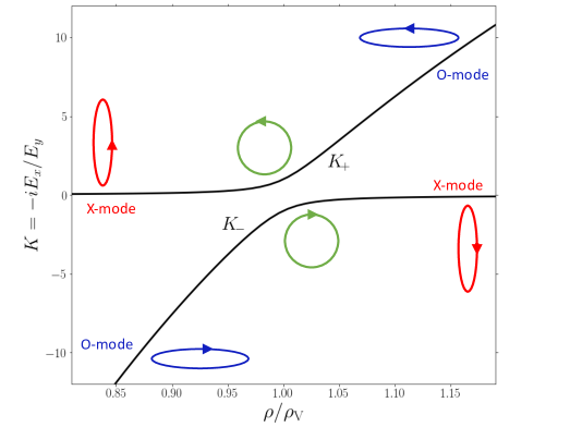
Figure 1: The polarization ellipticity of the photon mode as a function of density near the vacuum resonance. The two curves correspond to the (+) and (-) modes. In this example, the parameters are $B=10^{14}$G, $E=5\,$keV, and $\theta_{\rm kB}=30^{\circ}$. The ellipticity of a mode is specified by the ratio $K=-iE_{x}/E_{y}$, where $E_{x}$ ($E_{y}$) is the photon’s electric field component along (perpendicular to) the ${\bf k}$-${\bf B}$ plane. The O-mode is characterized by $|K|\gg 1$, and the X-mode $|K|\ll 1$.

When a photon propagates in an inhomogeneous medium, its polarization state will evolve adiabatically (i.e. following the $K_{+}$ or $K_{-}$ curve in Fig. 1) if the density variation is sufficiently gentle. Thus, a X-mode (O-mode) photon will be converted into the O-mode (X-mode) as it traverses the vacuum resonance, with its polarization ellipse rotated by $90^{\circ}$ (Fig. 1). This resonant mode conversion is analogous to the Mikheyev-Smirnov-Wolfenstein neutrino oscillation that takes place in the Sun [Haxton 1995, Bahcall et al. 2003] and similar level-crossing phenomena in other areas of sciences (e.g., Landau-Zener transition in atomic physics, EM wave propagation in inhomogeneous media and metamaterials; see Ref. [Tracy et al. 2014]). For this conversion to be effective, the adiabatic condition must be satisfied [Lai & Ho 2022]

$$E\gtrsim E_{\rm ad}=2.52\,\bigl{(}f\,\tan\theta_{\rm kB}\bigr{)}^{2/3}\!\left({1\,{\rm cm}\over H_{\rho}}\right)^{1/3}\!{\rm keV},$$ (5)

where $H_{\rho}=|ds/d\ln\rho|$ is the density scale height (evaluated at $\rho=\rho_{V}$) along the ray. In general, the probability for non-adiabatic “jump” is given by

$$P_{\rm J}=\exp\left[-{\pi\over 2}\Bigl{(}{E\over E_{\rm ad}}\Bigr{)}^{3}\right].$$ (6)

The mode conversion probability is $(1-P_{\rm J})$.

Calculation of Polarized Emission

To quantitatively compute the observed polarized X-ray emission from a magnetic NS, it is necessary to add up emissions from all surface patches of the star, taking account of beaming/anisotropy due to magnetic fields and light bending due to general relativity [Lai & Ho 2003a, van Adelsberg & Lai 2006, Zane 2006, Shabaltas & Lai 2012, Taverna et al. 2020, Caiazzon et al. 2022]. While this is conceptually straightforward, it necessarily involves many uncertainties related to the unknown distributions of surface temperature $T_{s}$ and magnetic field ${\bf B}$. In addition, the atmosphere composition is unknown, the opacity data for heavy atoms/ions for general magnetic field strengths are not available, and atmosphere models for many surface patches (each with different $T_{s}$ and ${\bf B}$) are needed. Finally, to determine the phase-resolved lightcurve and polarization, the relative orientations of the line of sight, spin axis and magnetic dipole axis are needed. Given all these complexities, we present a simplified, approximate calculation below. Our goal is to determine under what conditions (in term of the magnetic field strength, surface composition etc) the polarization swing can be produced.

We consider an atmosphere plasma composed of a single ionic species (each with charge $Ze$ and mass $Am_{p}$) and electrons. This is of course a simplification, as in reality the atmosphere would consist of multiple ionic species with different ionizations. With the equation of state $P=\rho kT/(\mu m_{p})$, hydrostatic balance implies that the column density $y$ at density $\rho$ is given by

$$y={\rho kT\over\mu m_{p}g}=0.41{\rho_{1}T_{6}\over\mu g_{2}}\,{\rm g/cm}^{2},$$ (7)

where $T=10^{6}\,T_{6}$ K is the temperature, $\mu=A/(1+Z)$ is the “molecular” weight, $\rho_{1}$ is the density in 1 g/cm³, and $g_{2}$ is the surface gravity $g=(GM/R^{2})(1-2GM/Rc^{2})^{-1}$ in units of $2\times 10^{14}$ (For $M=1.4M_{\odot}$, $R=12$ km, we have $g_{2}\simeq 1.00$). The density scale-height along a ray is

$$H_{\rho}\simeq{kT\over\mu m_{p}g\cos\alpha}=0.41\,{T_{6}\over\mu g_{2}\cos\alpha}\,{\rm cm},$$ (8)

where $\alpha$ is the angle between the ray and the NS surface normal.

To simplify our calculations, we shall neglect the electron scattering opacity and the bound-bound and bound-free opacities. The former is generally sub-dominant compared to the free-free opacity, while the latter are uncertain or unavailable. The free-free opacity of a photon mode (labeled by $i$) can be written as

$$\kappa_{i}=\kappa_{0}\xi_{i},$$ (9)

where the $B=0$ opacity is (setting the Gaunt factor to unity)

$$\kappa_{0}\simeq 9.3\,(Z^{3}/A^{2})\rho_{1}T_{6}^{-1/2}E_{1}^{-3}{\cal G},$$ (10)

with ${\cal G}=1-\exp(-E/kT)$. For the photon mode ${\bf E}\propto(iK,1)$, the dimensionless factor $\xi$ is given by [Ho & Lai 2002, Ho & Lai 2003]

$$\xi={K^{2}\sin^{2}\theta_{\rm kB}+(1+K^{2}\cos^{2}\theta_{\rm kB})/u_{e}\over 1+K^{2}}.$$ (11)

Figure 2 illustrates the behavior of $\xi_{X}$, $\xi_{O}$, $\xi_{+}$ and $\xi_{-}$ as a function of density. We see that for typical $\theta_{\rm kB}$’s, $\xi_{O}\sim 1$ and $\xi_{X}\sim u_{e}^{-1}\ll 1$ except near $\rho=\rho_{V}$.

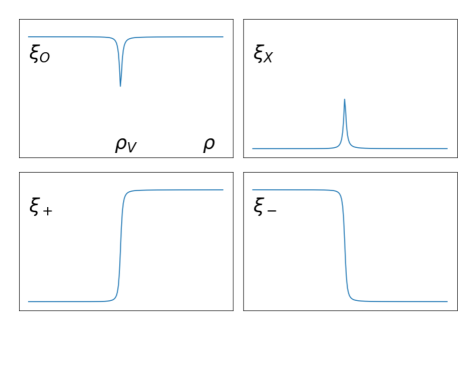
Figure 2: The qualitative behavior of $\xi_{i}$ (the dimensionless mode opacity; see Eq. 9) as a function of density for photon mode-$i$ (with $i={\rm X},{\rm O},+,-$). At the vacuum resonance ($\rho=\rho_{V}$), $\xi_{X}$ has a spike, $\xi_{O}$ has a dip, and $\xi_{+}$ and $\xi_{-}$ have discontinuities. Note that $\xi_{+}=\xi_{X}$ for $\rho<\rho_{V}$ and $\xi_{+}=\xi_{O}$ for $\rho>\rho_{V}$, while $\xi_{-}=\xi_{O}$ for $\rho<\rho_{V}$ and $\xi_{-}=\xi_{X}$ for $\rho>\rho_{V}$.

For a given photon energy $E$ and wave vector ${\bf k}$ (which is inclined by angle $\alpha$ with respect to the surface normal), the transfer equation for mode $i$ (with $i={\rm X},{\rm O}$ or $i=+,\,-$) reads

$$\cos\alpha{{\rm d}I_{i}\over{\rm d}y}=\kappa_{i}\left(I_{i}-{1\over 2}B_{\nu}\right),$$ (12)

where $B_{\nu}(T)$ is the Planck function and $T=T(y)$ is the temperature profile (to be specified later). To calculate the emergent polarized radiation intensity from the atmosphere, taking account of partial mode conversion, we adopt the following procedure [van Adelsberg & Lai 2006]: (i) We first integrate Eq. (12) for X-mode and O-mode ($i={\rm X},{\rm O}$) from large $y$ ($=\infty$) to $y_{V}$, the column density at which $\rho=\rho_{V}$. This gives $I_{\rm XV}$ and $I_{\rm OV}$, the X- and O-mode intensities just before resonance crossing. (ii) We apply partial mode conversion

$$I_{\rm XV}^{\prime}=I_{\rm XV}P_{J}+I_{\rm OV}(1-P_{J}),$$ (13)

$$I_{\rm OV}^{\prime}=I_{\rm OV}P_{J}+I_{\rm XV}(1-P_{J}),$$ (14)

to obtain the mode intensities just after resonance crossing. This partial conversion treatment is valid since the resonance width is small ($\Delta\rho/\rho_{V}\ll 1$; see Eq. 4). (iii) We then integrate Eq. (12) for X-mode and O-mode again from $y=y_{V}$ (with the ”initial” values $I_{\rm XV}^{\prime},I_{\rm OV}^{\prime}$) to $y\ll 1$. This then gives the mode intensities emergent from the atmosphere, $I_{X,e}$, $I_{O,e}$.

An alternative procedure is to integrate Eq. (12) for $i={\rm X},{\rm O},+,-$ from $y\gg 1$ to $y\ll 1$ (without applying partial mode conversion), which gives the intensities $I_{X}(0),I_{O}(0),I_{+}(0)$ and $I_{-}(0)$ at $y\simeq 0$. Then apply the partial conversion

$$I_{X,e}=I_{X}(0)P_{J}+I_{+}(0)(1-P_{J}),$$ (15)

$$I_{O,e}=I_{O}(0)P_{J}+I_{-}(0)(1-P_{J}),$$ (16)

where $P_{J}$ is evaluated at $y=y_{V}$.

It is straightforward to show that the above two procedures are equivalent. For example, after obtaining $I_{\rm XV}^{\prime}$, we can get the emergent X-mode intensity by

$$I_{X,e}=I_{\rm XV}^{\prime}\exp\left(-{\tau_{\rm XV}\over\cos\alpha}\right)+\Delta I_{\rm XV},$$ (17)

where $\tau_{\rm XV}=\int_{0}^{y_{V}}\kappa_{X}\,{\rm d}y$ is the optical depth of X-mode (measured along the surface normal) at $y=y_{V}$, and $\Delta I_{\rm XV}$ is the contribution to $I_{X,e}$ from the region $0<y<y_{V}$:

$$\Delta I_{\rm XV}=\int_{0}^{\tau_{\rm XV}/\cos\alpha}\!\!\!\exp\left(-{\tau_{X}\over\cos\alpha}\right){1\over 2}B_{\nu}(T)\,{{\rm d}\tau_{X}\over\cos\alpha}.$$ (18)

On the other hand, when integrating Eq. (12) for $i={\rm X}$ from $y\gg 1$ to $y\ll 1$, we obtain

$$I_{X}(0)=I_{\rm XV}\exp\left(-{\tau_{\rm XV}\over\cos\alpha}\right)+\Delta I_{\rm XV}.$$ (19)

Similarly,

$$I_{+}(0)=I_{\rm OV}\exp\left(-{\tau_{\rm XV}\over\cos\alpha}\right)+\Delta I_{\rm XV}.$$ (20)

It is easy to see that Eq. (17) together with Eq. (13) (the first procedure) and Eq. (15) with Eqs. (19)-(20) (the second procedure) yield the same emergent $I_{X,e}$.

Photosphere densities and Critical Field

Before presenting our sample results, it is useful to estimate the photosphere densities for different modes and the condition for polarization swing.

When the vacuum polarization effect is neglected ($\rho_{V}=0)$, $|\beta|\gg 1$ at all densities (for typical $\theta_{\rm kB}$’s not too close to 0), the $\xi$-factors for the O-mode ($|K|\gg 1$) and for the X-mode (with $|K|\ll 1$) are

$$\xi_{O}\simeq\sin^{2}\theta_{\rm kB},\quad\xi_{X}\simeq{1\over u_{e}\sin^{2}\theta_{\rm kB}}.$$ (21)

The photospheres of the O-mode and X-mode photons are determined by the condition

$$\int_{0}^{y_{O,X}}\!\kappa_{O,X}\,{{\rm d}y\over\cos\alpha}=2/3.$$ (22)

The corresponding photosphere densities can be estimated as

$$\rho_{O}=\xi_{O}^{-1/2}\rho_{0},$$ (23)

$$\rho_{X}=\xi_{X}^{-1/2}\rho_{0},$$ (24)

where the “zero-field” photosphere density is

$$\rho_{0}\simeq 0.59\,\left({\mu g_{2}\cos\alpha\over{\cal G}}\right)^{1/2}\!\left({E_{1}\over Z}\right)^{3/2}\!\biggl{(}{A\over T_{6}^{1/4}}\biggr{)}\,\,{\rm g\,cm}^{-3}.$$ (25)

The effect of the vacuum resonance on the radiative transfer depends qualitatively on the ratios $\rho_{V}/\rho_{O}$ and $\rho_{V}/\rho_{X}$, given by

$${\rho_{V}\over\rho_{O}}=\left({B\over B_{\rm OV}}\right)^{2},\quad{\rho_{V}\over\rho_{X}}={B\over B_{\rm XV}},$$ (26)

where

$$\!\!\!B_{\rm OV}=7.8\!\times\!10^{13}\left(\!{\mu g_{2}\cos\alpha\over Z{\cal G}E_{1}\sin^{2}\!\theta_{\rm kB}}\!\right)^{\!1/4}\!\!\left(\!{f\over T_{6}^{1/8}}\!\right){\rm G},$$ (27)

$$\!\!\!B_{\rm XV}=7.1\!\times\!10^{16}\left(\!{\mu g_{2}\cos\alpha\over Z{\cal G}E_{1}^{3}}\!\right)^{\!1/2}\!\!\left(\!{f^{2}\sin\theta_{\rm kB}\over T_{6}^{1/4}}\!\right){\rm G}.$$ (28)

Clearly, the condition $B\ll B_{\rm XV}$ or $\rho_{V}\ll\rho_{X}$ is satisfied for almost all relevant NS parameters of interest, while $B_{\rm OV}$ defines the critical field strength for the 90^∘ polarization swing (see Figs. 3-4): If $B\lesssim B_{\rm OV}$, the emergent radiation is dominated by the X-mode for $E\lesssim E_{\rm ad}$ and by the O-mode for $E\gtrsim E_{\rm ad}$; if $B\gtrsim B_{\rm OV}$, the X-mode is dominant for all $E$’s.

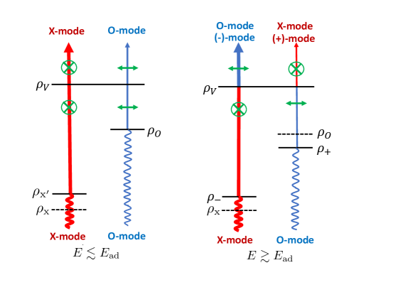
Figure 3: A schematic diagram illustrating how vacuum resonance affects the polarization state of the emergent radiation from a magnetized NS atmosphere. This diagram applies to the $B\lesssim B_{\rm OV}$ regime so that the vacuum resonance density $\rho_{V}$ is less than the O-mode photosphere density $\rho_{O}$. For $E\lesssim E_{\rm ad}$, the photon evolves nonadiabatically across the vacuum resonance (for $\theta_{\rm kB}$ not too close to $0$), thus the emergent radiation is dominated by the X-mode. For $E\gtrsim E_{\rm ad}$, the photon evolves adiabatically, with its plane of polarization rotating by 90^∘ across the vacuum resonance, and thus the emergent radiation is dominated by the O-mode. The plane of linear polarization at low energies is therefore perpendicular to that at high energies.

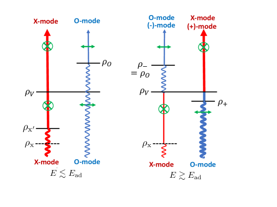
Figure 4: Same as Fig. 3, except for the $B\gtrsim B_{\rm OV}$ regime ($\rho_{V}>\rho_{O}$), in which the emergent radiation is always dominated by X-mode for all $E$’s.

We can quantify the role of $B_{\rm OV}$ more precisely by estimating how vacuum resonance affects the photosphere densities. In the limit of no mode conversion (i.e. $E\ll E_{\rm ad}$), it is appropriate to consider the transport of X-mode and O-mode, with the mode opacities modified around the vacuum resonance (see Fig. 2). The O-mode opacity has a dip near $\rho=\rho_{V}$ (where $\xi\simeq\sin^{2}\theta_{\rm kB}/2$), and since the resonance width $\Delta\rho/\rho_{V}\ll 1$, the photosphere density $\rho_{O^{\prime}}$ is almost unchanged from the no-vacuum value, i.e. $\rho_{O^{\prime}}\simeq\rho_{O}$. On the other hand, the X-mode opacity has a large spike at $\rho=\rho_{V}$ (where $\xi=\sin^{2}\theta_{\rm kB}/2$) compared to the off-resonance value ($\xi\sim u_{e}^{-1}$). The X-mode optical depth across the resonance (from $\rho_{V}-\Delta\rho$ to $\rho_{V}+\Delta\rho$) is of order $\Delta\tau_{V}\sim\epsilon(\rho_{V}/\rho_{O})^{2}$, where $\epsilon$ is given by Eq. (4). Thus the modified X-mode photosphere density is $\rho_{X^{\prime}}\simeq\rho_{V}$ for $\Delta\tau_{V}\gtrsim 1$ and

$$\rho_{X^{\prime}}\sim\rho_{X}\left[1-\epsilon\left({\rho_{V}/\rho_{O}}\right)^{2}\right]^{1/2}$$ (29)

for $\Delta\tau_{V}\lesssim 1$.

In the limit of complete mode conversion (i.e. $E\gg E_{\rm ad}$), it is appropriate to consider the transport of $(+)$-mode and $(-)$-mode, with the mode opacities exhibiting a discontinuity at $\rho=\rho_{V}$ (see Fig. 2). The $(+)$-mode photosphere density $\rho_{+}$ is given by

$$\rho_{+}^{2}\simeq\rho_{O}^{2}+\left(1+{\xi_{X}\over\xi_{O}}\right)\rho_{V}^{2}\simeq\rho_{O}^{2}+\rho_{V}^{2}.$$ (30)

The $(-)$-mode photosphere density $\rho_{-}$ is only affected by the vacuum resonance if $\rho_{O}>\rho_{V}$. Thus

$$\rho_{-}=\rho_{O}\qquad{\rm for}\leavevmode\nobreak\ \leavevmode\nobreak\ \rho_{O}<\rho_{V}$$ (31)

and

$$\rho_{-}^{2}=\rho_{V}^{2}+{\xi_{O}\over\xi_{X}}\left(\rho_{O}^{2}-\rho_{V}^{2}\right)\quad{\rm for}\leavevmode\nobreak\ \leavevmode\nobreak\ \rho_{O}>\rho_{V}$$ (32)

For general $E$’s with partial mode conversion, the emergent mode intensities are approximately given by

$$I_{O,e}\simeq{1\over 2}P_{J}B_{\nu}(\rho_{O})+{1\over 2}(1-P_{J})B_{\nu}(\rho_{-}),$$ (33)

$$I_{X,e}\simeq{1\over 2}P_{J}B_{\nu}(\rho_{X^{\prime}})P_{J}+{1\over 2}(1-P_{J})B_{\nu}(\rho_{+}),$$ (34)

where (for example) $B_{\nu}(\rho_{O})$ is the Planck function evaluated at $\rho=\rho_{O}$. These results are schematically depicted in Figs. 3-4.

Results

To compute the polarized radiation spectrum emergent from a NS atmosphere patch using the method presented above (Eq. 12 with Eqs. 13-14 or with Eqs. 15-16), we need to know the atmosphere temperature profile $T(y)$. This can be obtained only by self-consistent atmosphere modeling, which has only been done for a small number of cases (in terms of the local $T_{s}$, ${\bf B}$ and composition). Here, to explore the effect of different ${\bf B}$ and compositions, we consider two approximate models:

$\bullet$ Model (i): We use the profile $T_{\rm H}(y)$ for the $T_{s}=5\times 10^{6}$ K H atmosphere model with a vertical field $B=10^{14}$ G [see Fig. 5 and Eq. 48 of [van Adelsberg & Lai 2006]; this model correctly treats the partial model conversion effect], and re-scale it to take account of the modification of the free-free opacity for different $Z,\leavevmode\nobreak\ A$ (so that the re-scaled profile yields the same effective surface temperature $T_{s}$):

$$T(y)=\left({2\mu Z^{3}/A^{2}}\right)^{1/8.5}T_{\rm H}(y).$$ (35)

$\bullet$ Model (ii): We use a smooth (monotonic) fit to the $T_{\rm H}$ profile, given by

$$\log_{10}T_{\rm H}(y)=0.11+0.147\,\left[\,\log_{10}(0.4y)+3\,\right],$$ (36)

and then apply Eq. (35) for re-scaling.

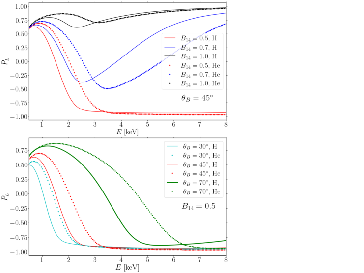
Figure 5: Polarization degree $P_{L}$ (defined by Eq. 37) of the emergent radiation normal to the surface as a function of the photon energy $E$ for H and He atmospheres with different magnetic field strengths and directions ($\theta_{B}$, the angle between the surface ${\bf B}$ and the surface normal vector). All results are based on the temperature profile Model (ii).

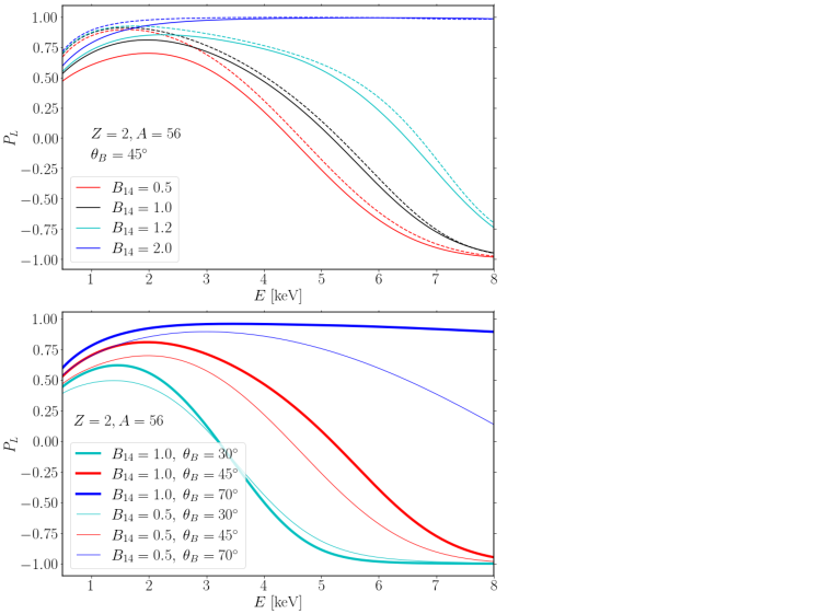
Figure 6: Similar to Fig. 5, except for partially ionized Fe atmospheres with $Z=2,\leavevmode\nobreak\ A=56$. In the upper panel, the solid/dashed lines are for Model (i)/(ii). In the lower panel, the results are shown for Model (i).

Figures 5-6 show a sample of our results for the polarization degree of the emergent radiation, defined by

$$P_{L}\equiv{I_{X,e}-I_{O,e}\over I_{X,e}+I_{O,e}}.$$ (37)

We see that for the H and He atmospheres (Fig. 5), $P_{L}$ transitions from being positive at low $E$’s to negative at high $E$’s for $B_{14}\lesssim 0.5$, in agreement with the critical field estimate (Eq. 27). The transition energy (where $P_{L}=0$) is approximately given by $E_{\rm ad}$, and has the scaling $E_{\rm ad}\propto(\mu\tan^{2}\theta_{B})^{1/3}$, where $\theta_{B}$ is the angle between the surface ${\bf B}$ and the surface normal (see Eq. 5). To obtain a transition energy of $4-5$ keV (as observed for 4U 0142) would require most of the emission comes from the surface region with $\theta_{B}\gtrsim 70^{\circ}$.

On the other hand, for a partially ionized heavy-element atmosphere (such that $\mu/Z$ is much larger than unity), the critical field $B_{\rm OV}$ can be increased (see Eq. 27). Figure 6 shows that at $B_{14}=1$, a $Z=2,\leavevmode\nobreak\ A=56$ atmosphere can have a sign change in $P_{L}$ around $E\sim 3-5$ keV (depending on the $\theta_{B}$ value.

To determine the observed polarization signal, we must consider the propagation of polarized radiation in the NS magnetosphere, whose dielectric property in the X-ray band is dominated by vacuum polarization [Heyl & Shaviv 2003]. As a photon propagates from the NS surface through the magnetosphere, its polarization state evolves following the varying magnetic field it experiences, up to the “polarization-limiting radius” $r_{\rm pl}$, beyond which the polarization state is frozen. It is convenient to set up a fixed coordinate system $XYZ$, where the Z-axis is along the line-of-sight and the $X$-axis lies in the plane spanned by the $Z$-axis and ${\bf\Omega}$ (the NS spin angular velocity vector). The polarization-limiting radius $r_{\rm pl}$ is determined by the condition $\Delta k=2|d\phi_{B}/ds|$, where $\Delta k=|k_{X}-k_{O}|$ is the difference in the wavenumbers of the two photon modes, and $\phi_{B}(s)$ is the azimuthal angle of the magnetic field along the ray ($s$ measures the distance along the ray). For a NS with surface dipole field $B_{d}$ and spin frequency $\nu=\Omega/(2\pi)$, we have [van Adelsberg & Lai 2006] ${r_{\rm pl}/R}\sim 150\,(E_{1}B_{d,14}^{2}/\nu_{1})^{1/6}$, where $B_{d,14}=B_{d}/(10^{14}\,{\rm G})$ and $\nu_{1}=\nu/{\rm Hz}$. Note that since $R\ll r_{\rm pl}\ll r_{l}$ [with $r_{l}=c/\Omega$ the light-cylinder radius), only the dipole field determines $r_{\rm pl}$. Regardless of the surface magnetic field structure, the radiation emerging from most atmosphere patches with mode intensities $I_{X,e}$ and $I_{O,e}$ evolves adiabatically in the magnetosphere such that the radiation at $r>r_{\rm pl}$ consists of approximately the same $I_{X,e}$ amd $I_{O,e}$, with a small mixture of circular polarization generated around $r_{\rm pl}$ [van Adelsberg & Lai 2006]. The exception occurs for those rays that encounter the quasi-tangential point (where the photon momentum is nearly aligned with the local magnetic field) during their travel from the surface to $r_{\rm pl}$ [Wang & Lai 2009]. Since only a small fraction of the NS surface radiation is affected by the quasi-tangential propagation, we can neglect its effect if the observed radiation comes from a large area of the NS surface. Let the azimuthal angle of the ${\bf B}$ field at $r_{\rm pl}$ be $\phi_{B}(r_{\rm pl})$ in the the $XYZ$ coordinate system. The observed Stokes parameters (normalized to the total intensity $I$) are then given by

$$Q/I=-P_{L}\cos 2\phi_{B}(r_{\rm pl}),$$ (38)

$$U/I=-P_{L}\sin 2\phi_{B}(r_{\rm pl}).$$ (39)

Note that when $r_{\rm pl}\ll r_{l}$, the transverse ($XY$) component of ${\bf B}(r_{\rm pl})$ is opposite to the transverse component of the magnetic dipole moment ${\bm{\mu}}$, thus $\phi_{B}(r_{\rm pl})\simeq\pi+\phi_{\mu}$, where $\phi_{\mu}$ is the azimuthal angle of ${\bm{\mu}}$.

For determine the emission from the whole NS surface, we need to add up contributions from different patches (area element ${\rm d}S$), inclduing the effect of general relativity [Pechenick et al. 1983, Beloborodov 2002]. For example, the observed spectral fluxes $F_{I},\leavevmode\nobreak\ F_{Q}$ (associated with the intensities $I,\leavevmode\nobreak\ Q$) are

$$F_{I}=g_{r}^{3}\int\!{{\rm d}S\,\cos\alpha\over D^{2}}(I_{X,e}+I_{O,e}),$$ (40)

$$F_{Q}=g_{r}^{3}\int\!{{\rm d}S\,\cos\alpha\over D^{2}}(I_{O,e}-I_{X,e})\cos 2\phi_{B}(r_{\rm pl}),$$ (41)

where $g_{r}\equiv(1-2GM/Rc^{2})^{1/2}$ and $\alpha$ is the angle between the ray and the surface normal at the emission point). Clearly, to compute $F_{I},\leavevmode\nobreak\ F_{Q}$ and $F_{U}$ requires the knowledge of the distributions of NS surface temperature and magnetic field, as well as various angles (the relative orientations between the line of sight, the spin axis and the dipole axis). This is beyond the scope of the paper. [Note that since $\phi_{B}(r_{\rm pl})\simeq\pi+\phi_{\mu}$, the phase variation of $F_{Q},\,F_{U}$ follows the rotation of the magnetic dipole, as in the rotating vector model.] Nevertheless, our results depicted in Figs. 5-6 (with different values of local field strengths and orientations) show that the 90^∘ linear polarization swing observed in AXP 4U 0142 can be explained by emission from a partially ionized heavy-element atmosphere with surface field strength about $10^{14}$ G, or a H/He atmosphere with $B_{14}\lesssim 0.5$ and a more restricted surface field geometry (i.e. most of the radiation comes from the regions with $\theta_{B}\gtrsim 70^{\circ}$).

Discussion

We have shown that the observed the x-ray polarization signal from AXP 4U 0142, particularly the 90^∘ swing around 4-5 keV, can be naturally explained by the mode conversion effect associated vacuum resonance in the NS atmosphere. In this scenario, the 2-4 keV emission is dominated by the X-mode, while the 5-8 keV emission by the O-mode as a result of the adiabatic mode conversion from the X-mode to the O-mode. This interpretation of the polarization swing would imply that the NS’s kick velocity is aligned with its spin axis, in agreement with the spin-kick correlation observed in other NS systems (see “Introduction”).

It is important to note that in our scenario, the existence of the X-ray polarization swing depends sensitively on the actual value of the magnetic field on the NS surface (see Eq. 27). To explain the observation of AXP 4U 0142, the magnetic fields in most region of the NS surface must be less than about $10^{14}$ G, and a lower field strength would be preferred in terms of producing the polarization swing robustly (for a wide range of geometrical parameters). Using the pulsar spindown power derived from force-free electrodynamics simulations [Spitkovsky 2006], $L_{\rm sd}=(\mu^{2}\Omega^{4}/c^{3})(1+\sin^{2}\theta_{s\mu})$ (where $\theta_{s\mu}$ is the angle between the magnetic dipole ${\bm{\mu}}$ and the spin axis), we find that for the observed $P,\,\dot{P}$ of 4U 0142, the dipole field at the magnetic equator is $B_{d}=1.1\times 10^{14}I_{45}^{1/2}R_{6}^{-3}(1+\sin^{2}\theta_{s\mu})^{-1/2}$ G, where $R_{6}$ is the NS radius in units of $10^{6}$ cm, and $I_{45}$ is the moment of inertia in units of $10^{45}$ g cm². Note that with $R_{6}\simeq 1.3$ [Miller et al. 2021, Raaijmakers et al. 2021], the above estimate is reduced by a factor of 2. In addition, if the magnetar possesses a relativistc wind with luminosity $L_{w}\gtrsim L_{\rm sd}$, the wind can open up field lines at $r_{\rm open}\sim(B_{d}^{2}R^{6}c/L_{w})^{1/4}\lesssim c/\Omega$ and significantly enhance the spindown torque [Thompson & Blaes 1998, Harding et al. 1999, Thompson et al. 2000]. This would imply that a smaller $B_{d}$ is needed to produce the observed $\dot{P}$ in 4U 0142. Thus, the observation of X-ray polarization swing is consistent with the indirectly “measured” dipole field, and requires that the high-order multipole field components be not much stronger than the dipole field.

We reiterate some of the caveats of our work: we have not attempted to calculate the synthetic polarized radiation from the whole NS and to compare with the X-ray data from AXP 4U 0142 in detail; our treatment of partially ionized heavy-element magnetic NS atmospheres is also approximate in several aspects (e.g., bound-free opacities are neglected, the vertical temperature profiles are assumed based on limited H atmosphere models). At present, these caveats are unavoidable, given the uncertainties (and large parameter space needed to do a proper survey) in the surface temperature and magnetic field distributions on the NS, and the fact that self-consistent heavy-element atmospheres models for general magnetic field strengths and orientations have not be constructed, especially in the regime where the vacuum resonance effects are important.

In this work, we have interpreted the 2-8 keV polarization signal from AXP 4U 0142 in terms of thermal emission from the NS surface. It is well established that for quiescent magnetars, the spectrum turns up above 10 keV, such that the bulk of their energy comes out as non-thermal hard X-rays [Kuiper et al. 2004, Kaspi & Beloborodov 2017]. The 0.5-10 keV spectrum can be parameterized either by an absorbed blackbody plus a power-law component (of photon index between $-4$ and $-2$) or by the sum of several blackbodies. So it is possible that the 5-8 keV emission from AXP 4U 0142 has a significant non-thermal contribution. Thompson & Kostenko [Thompson & Kostenko 2020] have studied a model in which the hard X-ray emission of quiescent magnetars comes from the “annihilation bremsstrahlung” of an electron–positron magnetospheric plasma. Such emission is mainly polarized in O-mode. If this emission dominates the 5-8 keV spectrum of APX 4U 0142 while negligible at lower energies, it could provide an alternative explanation for the polarization swing for a wide range of surface field strengths (recall that for $B\gtrsim B_{\rm OV}$, the atmosphere thermal emission is dominated by X-mode for all $E$’s (see eq. 27).

Very recently, while this paper is under review, IXPE reported the detection of polarized X-rays from another magnetar, 1RXS J170849.0-400910 [Zane et al. 2023]: The phase-averaged polarization signal exhibits an increase with energy, from $\sim 20\%$ at 2–3 keV to $\sim 80\%$ at 6–8 keV, while the polarization angle is independent of the photon energy. This constant polarization angle is consistent with atmospheric emission dominated by X-mode at all energies, and is expected since the measured dipole field (based on spindown) for this AXP, $B_{d}\simeq 5\times 10^{14}$ G, is significantly larger than $B_{\rm OV}$ (eq. 27). The increase of linear polarization with $E$ can be a result of the magnetic field geometry (relative to the spin axis and line-of-sight) and the surface temperature distribution [see Ref. [van Adelsberg & Lai 2006] for examples].

Overall, our work demonstrates the important role played by the vacuum resonance in producing the observed X-ray polarization signature from magnetars (and NSs with weaker magnetic fields). The observations of AXP 4U 0142 and 1RXS J170849.0-400910 by IXPE have now opened up a new window in studying the surface environment of NSs. Future X-ray polarization mission [such as eXTP; see Ref. [Zhang et al. 2019]] will provide more detailed observational data. Comprehensive theoretical modelings of magnetic NS surface radiation and magnetosphere emission will be needed to confront these observations.

Acknowledgements: We thank Chris Thompson for useful discussion. This work is supported in part by Cornell University.

References

- [Thompson & Duncan 1993] Thompson, C., Duncan R. C. 1993, Neutron star dynamos and the origins of pulsar magnetism, ApJ, 408, 194
- [Kaspi & Beloborodov 2017] Kaspi V. M., Beloborodov A. M., 2017, Magnetars, ARA&A, 55, 261
- [Weisskopf et al. 2016] Weisskopf, M.C. et al. 2016, The imaging x-ray polarimetry explorer (IXPE), Proc. SPIE 9905, 990517; https://doi.org/10.1117/12.2235240
- [Taverna et al. 2022] Taverna, R. et al. 2022, Polarized x-rays from a magnetar, Science, 378, 646
- [Medin & Lai 2007] Medin, Z., Lai, D. 2007, Condensed surfaces of magnetic neutron stars, thermal surface emission, and particle acceleration above pulsar polar caps, MNRAS, 382, 1833
- [Potekhin & Chabrier 2013] Potekhin, A., Chabrier, G. 2013, Equation of state for magnetized Coulomb plasmas, A&A, 550, A43
- [Medin & Lai 2006] Medin, Z., Lai, D. 2006, Density-functional-theory calculations of matter in strong magnetic fields. II. Infinite chains and condensed matter, Phy. Rev. A 74, 062508
- [van Adelsberg et al. 2005] van Adelsberg, M., Lai, D. Potekhin, A.Y., Arras, P. 2005, Radiation from condensed surface of magnetic neutron stars, ApJ, 628, 902
- [Potekhin et al. 2012] Potekhin, A.Y., Suleimanov, V.F., van Adelsberg, M., Werner, K. 2012, Radiative properties of magnetic neutron stars with metallic surfaces and thin atmospheres, A&A, 546, A121
- [Lai et al. 2001] Lai, D., Chernoff, D.F., Cordes, J.M. 2001, Pulsar jets: implications for neutron star kicks and initial spins, ApJ, 549, 1118
- [Johnston et al. 2005] Johnston, S., et al. 2005, Evidence for alignment of the rotation and velocity vectors in pulsars, MNRAS, 364, 1394
- [Wang et al. 2006] Wang, C., Lai, D., Han, J.L. 2006, Neutron Star Kicks in Isolated and Binary Pulsars: Observational Constraints and Implications for Kick Mechanisms, ApJ, 639, 1007
- [Noutsos et al. 2013] Noutsos, A., et al. 2013, Pulsar spin–velocity alignment: kinematic ages, birth periods and braking indices, MNRAS, 430, 2281
- [Janka et al. 2022] Janka, H.-T., Wongwathanarat, A., Kramer, M. 2022, Supernova fallback as origin of neutron star spins and spin-kick alignment, ApJ, 926, 9
- [Lai & Ho 2003a] Lai, D., Ho, W.C.G. 2003a, Polarized X-ray emission from magnetized neutron stars: signature of strong-field vacuum polarization, PRL, 91, 071101
- [Zane et al. 2023] Zane, S., et al. 2023, A strong X-ray polarization signal from the magnetar 1RXS J170849.0-400910, ApJ, arXiv:2301.12919
- [Heisenberg & Euler 1936] Heisenberg, W. & Euler, H. 1936, Folgerungen aus der Diracschen Theorie des Positrons, Z. Physik, 98, 714
- [Schwinger 1951] Schwinger, J. 1951, On Gauge Invariance and Vacuum Polarization, Phys. Rev., 82, 664
- [Adler 1971] Adler, S.L. 1971, Photon Splitting and Photon Dispersion in a Strong Magnetic Field, Ann. Phys., 67, 599
- [Tsai & Erber 1975] Tsai, W.Y., Erber, T. 1975, Propagation of photons in homogeneous magnetic fields: Index of refraction, Phys. Rev. D, 12, 1132
- [Heyl & Hernquist 1997] Heyl, J.S. & Hernquist, L. 1997, Birefringence and dichroism of the QED vacuum, J. Phys. A 30, 6485
- [Gnedin et al. 1978] Gnedin, Yu.N., Pavlov, G.G., & Shibanov, Yu.A. 1978, The Effect of Vacuum Birefringence in a Magnetic Field on the Polarization and Beaming of X-ray Pulsars, Sov. Astron. Lett., 4(3), 117
- [Mészáros & Ventura 1979] Mészáros, P. & Ventura, J. 1979, Vacuum polarization effects on radiative opacities in a strong magnetic field, Phys. Rev. D 19, 3565
- [Pavlov & Gnedin 1984] Pavlov, G.G. & Gnedin, Yu.N. 1984, Vacuum Polarization by a Magnetic Field and its Astrophysical Manifestations, Sov. Sci. Rev. E: Astrophys. Space Phys. 3, 197
- [Lai & Ho 2022] Lai, D., Ho, W.C.G. 2002, Resonant Conversion of Photon Modes Due to Vacuum Polarization in a Magnetized Plasma: Implications for X-Ray Emission from Magnetars, ApJ, 566, 373
- [Ho & Lai 2003] Ho, W.C.G., & Lai, D. 2003, Atmospheres and Spectra of Strongly Magnetized Neutron Stars II: Effect of Vacuum Polarization, MNRAS, 338, 233
- [Lai & Ho 2003b] Lai, D., Ho, W.C.G. 2003b, Transfer of Polarized Radiation in Strongly Magnetized Plasmas and Thermal Emission from Magnetars: Effect of Vacuum Polarization, ApJ, 588, 962
- [Mészáros 1992] Mészáros, P. 1992, High-Energy Radiation from Magnetized Neutron Stars (Univ. Chicago Press, Chicago)
- [Potekhin et al. 2004] Potekhin, A., et al. 2004, Electromagnetic Polarization in Partially Ionized Plasmas with Strong Magnetic Fields and Neutron Star Atmosphere Models, ApJ, 612, 1034
- [Haxton 1995] Haxton, W.C. 1995, The Solar Neutrino Problem, Ann. Rev. Astron. Astrophys., 33, 459
- [Bahcall et al. 2003] Bahcall, J.N., Gonzalez-Garcia, M.C., & Pena-Garay, C. 2003, Solar Neutrinos Before and After KamLAND, J. High Energy Phys. JHEP02, 009
- [Tracy et al. 2014] Tracy, E.R., et al. 2014, Ray Tracing and Beyond: Phase Space Methods in Plasma Wave Theory (Cambridge Univ.)
- [van Adelsberg & Lai 2006] van Adelsberg, M., Lai, D. 2006, Atmosphere models of magnetized neutron stars: QED effects, radiation spectra and polarization signals, MNRAS, 373, 1495
- [Zane 2006] Zane, S., & Turolla, R. 2006, Unveiling the thermal and magnetic map of neutron star surfaces though their X-ray emission: method and light-curve analysis, MNRAS, 366, 727
- [Shabaltas & Lai 2012] Shabaltas, N., Lai, D. 2012, The hidden magnetic fields of the young neutron star in Kes 79, ApJ, 748, 148
- [Taverna et al. 2020] Taverna, R., Turolla, R., Suleimanov, V., Potekhin, A.Y., Zane, S. 2020, X-ray spectra and polarization from magnetar candidates, MNRAS, 492, 5057
- [Caiazzon et al. 2022] Caiazzo, I., Gonzalez-Caniulef, D., Heyl, J., Fernandez, R. 2022, Probing magnetar emission mechanisms with X-ray spectropolarimetry, MNRAS, 514, 5024
- [Ho & Lai 2002] Ho, W.C.G. & Lai, D. 2001, Atmospheres and spectra of strongly magnetized neutron stars, MNRAS, 327, 1081
- [Heyl & Shaviv 2003] Heyl, J.S., Shaviv, N.J., & Lloyd, D. 2003, The High-Energy Polarization-Limiting Radius of Neutron Star Magnetospheres I – Slowly Rotating Neutron Stars, MNRAS, 342, 134
- [Wang & Lai 2009] Wang, C., Lai, D. 2009, Polarization evolution in a strongly magnetized vacuum: QED effect and polarized X-ray emission from magnetized neutron stars, MNRAS, 398, 515
- [Pechenick et al. 1983] Pechenick, K.R., Ftaclas, C., & Cohen, J.M. 1983, Hot Spots on Neutron Stars: The Near-Field Gravitational Lens, ApJ, 274, 846
- [Beloborodov 2002] Beloborodov, A.M. 2002, Gravitational Bending of Light Near Compact Objects, ApJ, 566, L85
- [Spitkovsky 2006] Spitkovsky, A. 2006, Time-dependent Force-free Pulsar Magnetospheres: Axisymmetric and Oblique Rotators, ApJ, 648, L51
- [Miller et al. 2021] Miller, M.C. et al. 2021, The radius of PSR J0740+ 6620 from NICER and XMM-Newton data, ApJ, 918, L28
- [Raaijmakers et al. 2021] Raaijmakers, G. et al. 2021, Constraints on the Dense Matter Equation of State and Neutron Star Properties from NICER’s Mass–Radius Estimate of PSR J0740+6620 and Multimessenger Observations, ApJ, 918, L29
- [Thompson & Blaes 1998] Thompson C., Blaes O., 1998, Magnetohydrodynamics in the extreme relativistic limit, Phys. Rev. D 57, 3219
- [Harding et al. 1999] Harding A. K., Contopoulos I., Kazanas D., 1999, Magnetar spin-down, ApJ, 525, L125
- [Thompson et al. 2000] Thompson C., Duncan R. C., Woods P. M., Kouveliotou C., Finger M. H., van Paradijs J., 2000, Physical mechanisms for the variable spin-down and light curve of SGR 1900+14, ApJ, 543, 340
- [Kuiper et al. 2004] Kuiper L., Hermsen W., Mendez M. 2004, Discovery of hard nonthermal pulsed X-ray emission from the anomalous X-ray pulsar 1E 1841–045, ApJ, 613, 1173
- [Thompson & Kostenko 2020] Thompson C., Kostenko A. 2020, Pair plasma in super-QED magnetic fields and the hard X-ray/optical emission of magnetars, ApJ, 904, 184
- [Zhang et al. 2019] Zhang, Shuangnan, et al. 2019, The enhanced X-ray Timing and Polarimetry mission—eXTP, Science China Physics, Mechanics & Astronomy, 62, 29502