Intercepting A Flying Target While Avoiding Moving Obstacles: A Unified Control Framework With Deep Manifold Learning

Abstract

Real-time interception of a fast-moving object by a robotic arm in cluttered environments filled with static or dynamic obstacles permits only tens of milliseconds for reaction times, hence quite challenging and arduous for state-of-the-art robotic planning algorithms to perform multiple robotic skills, for instance, catching the dynamic object and avoiding obstacles, in parallel. This paper proposes an unified framework of robotic path planning through embedding the high-dimensional temporal information contained in the event stream to distinguish between safe and colliding trajectories into a low-dimension space manifested with a pre-constructed 2D densely connected graph. We then leverage a fast graph-traversing strategy to generate the motor commands necessary to effectively avoid the approaching obstacles while simultaneously intercepting a fast-moving objects. The most distinctive feature of our methodology is to conduct both object interception and obstacle avoidance within the same algorithm framework based on deep manifold learning. By leveraging a highly efficient diffusion-map based variational autoencoding and Extended Kalman Filter(EKF), we demonstrate the effectiveness of our approach on an autonomous 7-DoF robotic arm using only onboard sensing and computation. Our robotic manipulator was capable of avoiding multiple obstacles of different sizes and shapes while successfully capturing a fast-moving soft ball thrown by hand at normal speed in different angles.

Complete video demonstrations of our experiments can be found in https://sites.google.com/view/multirobotskill/home.

I Introduction

Real-time response and minimal reactive time is crucial to the robotic motion planning and online control of target-directed reaching movements in dynamic and cluttered environments. Specifically, intercepting a flying object in the real world is quite different from typical robotic reaching movements studied in the typical laboratory setting in two important respects. First, the targets for capturing in the real world often move at a high speed, and second, the workspace in the real world is often cluttered with many dynamic obstacles that are moving and changing in their geometric forms. It becomes quite expensive to afford any perception latency[1] while performing real-time robotic skill execution such as high-speed target catching while operating in a convoluted environment with static or dynamic obstacles. In this work, we aimed to develop a unified framework for learning multiple robotic skills in parallel for real-time operation. Through learning a low-dimensional geometrical manifold represenation based on diffusion map[2], this research work proposed a unique methodology to intercept a fast-moving target by redundant robotic manipulators while avoiding dynamic obstacles present in the environment. Although the effects of changes in target position[3, 4, 5] and the effects of dynamic obstacles[6, 7, 8] have been investigated separately in the literature, there have been few studies looking at them together[9]. Besides, latent space representation and manifold learning has been previously exploited for learning robotic skills[10, 11], but with concentration on solving one particular robotic skill. The main objective of this work, therefore, was to integrate both deep manifold learning and EKF in order to achieve algorithm simplicity and computing efficiency for real-time interceptive tasks with dynamic obstacle avoidance.

In this paper, we have proposed a unified and innovative topological manifold learning approach for dynamic target interception and collision avoidance by a 7-DOF research-grade robotic manipulator. The contributions of this work can be highlighted as,

• We utilized here EKF for accurately estimating the location of the moving target in the reachable workspace of the robotic arm.

• Through a fusion of diffusion map and variational autoencoding, we learned a 2D manifold representation of high-dimensional robotic state vector which in turn reveals the system dynamics of robotic manipulator and point obstacle in low-dimensional space.

• We constructed a densely-connected graph network over the learned 2D manifold data-points which greatly facilitated the motion planning in the shortest possible path and time by efficiently performing graph traversing on the collision-free vertices.

• In parallel of obstacle avoidance, we implemented here target catching scheme by nearest neighborhood look-up of predicted target location in end-effector’s positions inside respective transformed manifold datapoints.

We have demonstrated both in simulated environment and real-world robotic setup the efficacy and real-time performance of our proposed approach. The most promising advantage of our methodology is its generalization capability to handle any number of obstacles and intercept a moving target with real-time trajectory execution.

II Preliminaries

Diffusion Map : Diffusion map (DM) is well-known non-linear dimensionality reduction algorithm which computes set of low-dimensional embeddings of high-dimensional dataset with a focus on uncovering the underlying geometrical properties[2, 12, 13]. DM is based upon the relationship between time-scaled diffusion process over the data space, $\mathbb{X}$ and random walk Markov Chain. The probability of randomly walking from $x\in\mathbb{X}$ to $y\in\mathbb{X}$ is computed through diffusion kernel, $k(x,y;\alpha):\mathbb{X}\times\mathbb{X}\rightarrow\mathbb{R}$, $k(x,y;\alpha)=\exp(-\frac{|x-y|^{2}}{\alpha})$ and probability of walking between adjacent points $p(x,y)=k(x,y)/d(x)$ where $d(x)=\int_{\mathbb{X}}k(x,y)d\mu(y)$ and $\mu$ represents the distribution of samples in data space $\mathbb{X}$. With the computation of $p(x_{i},y_{j})$, diffusion process determines the normalised diffusion matrix $P^{t}_{ij}$ where each entry represents the sum of all paths of length $t$ from any point $i$ to $j$. With the increasing value of $t$, the probability of traversing among close neighboring points escalates which indirectly form the global geometry of the data[13]. Diffusion process paves the way for defining Diffusion distance,

$$D_{t}(X_{i},X_{j})^{2}=\underset{k}{\sum}|P^{t}_{ik}-P^{t}_{kj}|^{2}$$ (1)

$D_{t}(X_{i},X_{j})^{2}$ evaluates the similarity between the sample points in the data space which inherently clusters the closest point together in manifold representation learned through diffusion maps. In this work, diffusion map is primarily utilized for dimensionality reduction from high robotic state-space to latent space manifold representation. The diffusion metric organises the data maintaining close proximity and lower-dimensional structure carries all necessary geometric intrinsic properties of original dataset. Computation of diffusion distance in the original high-dimensional robotic space is computationally expensive. Moreover, the euclidean distance after diffusion mapping of the data is equivalent to the diffusion distance in original data-space[13], i.e

$$D_{t}(X_{i},X_{j})^{2}=||Y_{i}-Y_{j}||^{2}_{E}$$ (2)

The dimensionality reduction in diffusion mapping happens by decomposing the mapping functionals $Y_{i}$ into eigenfunctions of diffusion matrix $P$ and eigenvalues $\lambda_{i}$. Through considering first $d$ dominant eigenvalues, we finalize the dimensionality reduction i.e $\mathbb{X}\in\mathbb{R}^{m}\rightarrow\mathcal{M}_{z}\in\mathbb{R}^{d}\;\text{where}\;d<m$.

Variational Diffusion Autoencoders : Classical non-linear dimensionality reduction techniques such as Isomap or DM do not easily provide a mechanism of doing inverse mapping from mapped diffusion coordinates to original data space. On the contrary, state-of-the-art deep learning based generative models such as Variational Autoencoder (VAE)[14] have exhibited astronomical success in image and text generation through learning a latent-space representation. Specifically, in our work, we opted to apply VAE for performing the inverse diffusion map operation and reconstructing the joint-space configuration of robotic manipulator from the encoded manifold space representation. In our work, 2D manifold datapoints are converted into a 2D fully connected network, $\mathcal{G}$ on which we traversed to any target vertice $V_{tar}$ by shortest path routing. The connecting vertices $V_{i}$ on the shortest path were required to be remapped to original data distributions for planning motion in joint-space and executing the joint commands to move the robotic arm to a preset or predicted target location in $\mathbb{R}^{3}$ space. In parallel, we aimed at proposing a real-time obstacle avoidance algorithm through revising the initial routed path on same 2D connected graph and upgrading to the next best shortest path to deftly avoid occlusions perturbing the initial trajectory. Since, in our robotic trajectory planning approach, we apparently aimed to infer distinctive joint-space data for each manifold datapoint, we could hardly allow any posterior collapse in our VAE optimization procedures. Posterior collapse occurs when the learned mapping converts large pools of input dataset into a single output point (more details in [15]). This phenomena seriously violates the bijective homeomorphic property expected from manifold learning[16].

To mitigate above challenges related to VAE and to integrate inverse diffusion mapping with traditional diffusion map based manifold learning, [16] proposed variational diffusion autoencoders which binded the blessings of both manifold learning to encapsulate geometrical properties into a low-dimensional representation and, VAE to implement inverse diffusion map through a random walk sampling in close neighborhood of a point of original dataset. The conventional reconstruction error based optimization procedure of a VAE is modified in VDAE as,

$$\mathcal{L}_{VDAE}=-D_{KL}(f_{\omega}(z^{\prime}|x)||p_{\phi}(z^{\prime}|x))+\log p_{\phi}(x^{\prime}|z^{\prime}_{i})$$ (3)

The first term in above loss function defines divergence from true diffusion probabilities through computing Kullback–Leibler divergence between true diffusion distribution $p_{\phi}(z^{\prime}|x)$ and approximated diffuston random walk based distribution $f_{\omega}(z^{\prime}|x)$. The second term maximizes the log-likelihood probability of new-point $x^{\prime}$ conditioned on the learned latent space representation. VDAE ensures that new point $x^{\prime}$ is sampled from closed neighborhood of the test data point $x$ with respect to the similarity metric in diffusion space. In our work, we have modified the 2nd term related to reconstruction error with more straightforward L2-norm based loss function which eases the optimization procedures. Moreover, we have used decoder network of VDAE to reconstruct the joint-space control signal for our shortest path vertices to plan a smooth motion.

III Proposed Methodology

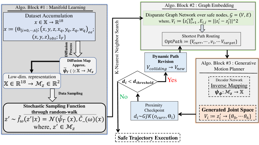
Figure 1: Algorithmic block diagram of our overall methodology.

Fig.1 depicts the structure of our proposed methodology related to manifold learning and graph traversing. It consists of three major algorithm modules: 1) diffusion map based manifold learning which transforms high-dimensional robotic information into low-dimensional 2D manifold points, in order to facilitate robotic path planning to reach a dynamic target location and perform obstacle avoidance in parallel, 2) variational decoding, which bridges between high-dimensional robotic poses and low-dimensional manifold spaces for instantly transforms the low-dimensional diffusion space to high-dimensional data space, and 3) fully connected network graph constructed with 2D mapped points, and dynamic routing through optimum paths to target location while concurrently performing obstacle avoidance.

III-A Manifold Learning Through Variational Diffusion Autoencoding

Diffusion Map is a well-known classical non-linear dimensionality reduction techniques for learning geometric manifold space for a domain-specific high-dimensional data space. As the time-dependent diffusion process advances, the local geometrical properties of high-dimensional data space get revealed inside the manifold representation[16, 2]. To learn the manifold representation through Diffusion Maps, we have utilized here variational diffusion autoencoder (VDAE)[16] which efficiently proposed a fusion of variational inference and diffusion maps. Given a data space $\mathbb{X}$, sample observations $x_{i}\subseteq\mathbb{X}$ and a predefined Gaussian diffusion kernel $k_{d}(x_{i},x_{j})$, the VDAE encodes geometrical properties of euclidean space $\mathbb{X}$ into low-dimensional manifold space $\mathcal{M}_{Z}:=\widetilde{\psi}_{\Gamma}(\mathbb{X})$. This encoding scheme is largely designed with Spectralnet[17] which is deep neural network based approximators parameterized by $\Gamma$ to model the diffusion map feature space $\widetilde{\psi}_{\Gamma}(\cdot)$. In this work, our high-dimensional data space consisted of 18 floating numbers. Each sample of dataset was defined by $[\theta_{0},\cdots,\theta_{6};\{x,y,z,x_{q},y_{q},z_{q},w_{q}\}_{ee};\{x,y,z\}_{o};\mathbb{I}_{F}]$, where $\theta_{i}$s determining the exact full joint-space pose of a robotic arm; $\{x,y,z,x_{q},y_{q},z_{q},w_{q}\}_{ee}$ representing end-effector’s coordinates and orientations in quaternion; $\{x,y,z\}_{o}$ defining the location of a point obstacle; $\mathbb{I}_{F}$ which is boolean collision flag. One critical aspect of our considered high-dimensional space is that it poses the complex system dynamic and geometrical properties between any full pose of a chosen robotic arm and a point obstacle at arbitrary, but valid configuration.

Secondly, we learnt the stochastic sampling function $\widetilde{f}_{\omega}(z^{\prime}|x)\rightarrow z^{\prime}$ which is defined by a Gaussian Normal distribution, $\mathcal{N}(\widetilde{\psi}_{\Gamma}(x),\widetilde{C}_{\omega}(x))$ following [16]. Here, $\widetilde{C}_{\omega}(x)$ defines the co-variance matrix of the random walk on manifold space $\mathcal{M}_{Z}$ for any sample $x_{i}$. Once, the learning of parametric space $\omega$ for $\widetilde{C}_{\omega}(\cdot)$ and manifold learning through SpectralNet converges, we stored the low-dimensional manifold data $z^{\prime}$ in 2D space by considering only first two dominant eigenfunctions[13] and $\{z^{\prime}_{i}\}_{i=1}^{N}$, where $N=\#\;of\;samples$, were utilized to form a connected network in 2D for real-time motion planning over the manifold space.

III-B Generative Motion Planner Variational Decoding

To facilitate our manifold-based robotic motion planning for obstacle avoidance, we need to seamlessly transform between high-dimensional robotic space, $\mathbb{X}$ and low-dimensional manifold space, $\mathcal{M}_{z}$. For this, we used the decoder part of the VDAE architecture. Most of the non-linear dimensionality reduction techniques such as diffusion map does not have straightforward inverse diffusion map operation. Here, encoded manifold data was inversely transformed to original data distributions through using decoding function approximator, $\psi_{\phi}:=\mathcal{M}_{z}\rightarrow\mathbb{X}$ parameterized by $\phi$. Here, instead of using evidence maximization optimization (i.e log likelihood of $p_{\phi}(x^{\prime}|x)$) in [16], we used a straightforward L2-norm based optimization to inversely map the high-dimensional samples from latent space manifold. The loss function is $\mathcal{L}_{dec}\approx\underset{\omega,\phi}{\operatorname*{arg\,min}}||x-\psi_{\phi}(z^{\prime})||^{2},\;\text{where}\;z^{\prime}\sim\widetilde{f}_{\omega}(\cdot|x)$. This mapping could be considered as one-to-one function between input and output layers, because we aimed to generate motion planning through approximating unique joint-space configuration, $\Theta^{\prime}_{i}$ of robotic arm for a respective low-dimensional representation $z^{\prime}_{i}$. Our decoder network is trained through backpropagation of the reconstruction error. Once the learning converges, we can coherently plan an adaptive robotic trajectory execution through generating joint-configuration from the low-dimensional manifold space.

III-C Densely Connected Graph In Manifold Space and Shortest Path Routing

Diffusion map centric graph construction and optimal routing through connected graphs for real world navigation and motion planning has been well established with a view to learning obstacle avoidance[18, 19] and visual navigation[20]. However, such graph based planning has been largely employed in mobile robots maneuvering on 2D-planar Euclidean space. On the contrary, the graph, $\mathcal{G}$ we constructed in $\mathbb{R}^{2}$ space encodes the geometric intrinsics from $\mathbb{R}^{3}\times\mathcal{S}^{3}$ space of a redundant robotic manipulator operating against point obstacles in $\mathbb{R}^{3}$ and represents the dynamic relationship embedded in a topological manifold space. In our study, we opted to use 2D low-dimensional latent space representation to simplify our graph data structure and its traversing algorithms. The Graph, $\mathcal{G}=(V,E)$ consisted of $V_{\{i=1,\cdots,n\}}\in\mathcal{M}_{z}$ nodes associated with respective high-dimensional samples, $X_{\{i=1,\cdots,n\}}$. Specifically, after our manifold learning converges , we stamped the encoded low-dimensional mappings either as “collision” or “collision free/safe” vertice based on the respective $\mathbb{I}_{F}$. A fully connected network was built through nearest neighbor search on each “safe” node and our methodology performed a shortest routing algorithm for reaching a predicted target node, $V_{tar}$ and the dense connectivity was also exploited to upgrade the previous routing for avoiding any dynamic or static obstacles preventing the robot motion. Moreover, edges in the network $E$ were weighted by Euclidean distance in diffusion space between adjacent nodes, since diffusion distance in original data space is equivalent to Euclidean distance in diffusion space[13]. The decoder effectively generated the control sequence for motion planning from the planned route and connected nodes on the route. To reduce latency on graph based computation, we designed graph internal data structures on an adjacency list representation and implemented using Python dictionary data structures. Furthermore, the graph adjacency structure is implemented as a Python dictionary of dictionaries; the outer dictionary is keyed by nodes to values that are themselves dictionaries keyed by neighboring node to the edge attributes associated with that edge. This “dict-of-dicts” structure allows fast addition, deletion, and lookup of nodes and neighbors in large graphs. All of our functions manipulate graph-like objects solely via predefined API methods and not by acting directly on the data structure. Our software code is largely based on the open-source NetworkX package[21].

III-D Target Tracking through Extended Kalman Filter

We can consider a vector $s\in\mathbb{R}^{n}$ consisting of $n$ features on each frame captured by our vision sensor for target tracking. In case of Image based Visual Servoing (IBVS), these features can be determined as pixel coordinates $(f_{x},f_{y})$ on RGB frames and depth values $Z$ of respective coordinate from aligned depth frames. We opted here to use a eye-to-hand system for IBVS. In case of a hand-to-eye system, the kinematic relationship between motion of image features $\dot{s}$ and robot control (expressed as velocity screw, $v^{r}$) is determined by the image Jacobian or interaction matrix $L_{s}$[22]. Following [5], for eye-to-hand system, $v^{r}$ can be defined as the relative difference between end-effector velocity $v^{r}_{ee}$ in robot-frame, $r_{f}$ and target velocity $v^{c}_{o}$ in camera frame, $c_{f}$. The second term, $\dot{s}_{o}$ in Eq.(4) represents the unknown feature velocity.

$$\small\dot{s}=L_{s}v^{r}=L_{s}(v^{r_{f}}_{ee}-v^{c_{f}}_{o})=L_{s}v^{r_{f}}_{ee}-\dot{s}_{o}$$ (4)

$v^{r_{f}}_{ee}$ can be expressed with joint velocities $\dot{\Theta}$ through using Jacobian Matrix, $J_{ee}$ and Eq.(4) can be converted as,

$$\small\dot{s}=L_{s}{}^{c_{f}}\mathbb{T}_{r_{f}}J_{ee}\dot{\Theta}-\dot{s}_{o}$$ (5)

where ${}^{c_{f}}\mathbb{T}_{r_{f}}$ is the twist transformation matrix that transforms end-effector twist from $r_{f}$ to $c_{f}$.

In our study, the continuous-time state of the filter was defined as $x(t)=[s(t),z(t)]=[x_{1}(t),x_{2}(t)]$ where $s(t):=(f_{x},f_{y})$ and focal length, $\lambda$ of the vision sensor is known from the intrinsic properties of the sensor. The interaction matrix for $(f_{x},f_{y})$ is defined by[23, 24]

$$\scriptsize L_{s}(f_{x},f_{y},Z)=\begin{bmatrix}-\frac{\lambda}{Z}&0&\frac{f_{x}}{Z}&\frac{f_{x}f_{y}}{\lambda}&-(\lambda+\frac{f_{x}^{2}}{\lambda})&f_{y}\\ 0&-\frac{\lambda}{Z}&\frac{f_{y}}{Z}&\lambda+\frac{f_{y}^{2}}{\lambda}&-\frac{f_{x}f_{y}}{\lambda}&-f_{x}\end{bmatrix}$$ (6)

Also, the interaction matrix for depth estimate is given by[24],

$$\scriptsize L_{Z}(f_{x},f_{y},Z)=\begin{bmatrix}0&0&-1&-\frac{f_{y}Z}{\lambda}&-\frac{f_{x}Z}{\lambda}&0\\ \end{bmatrix}$$ (7)

and depth estimate, $\dot{Z}=L_{Z}v^{r}$. Unlike [5], here we have designed a hand-to-eye system. As a result, the interaction matrix is required to consider the rotational mapping, $R$ and translation vector, $t$ into $L_{s}$. For hand-to-eye system, the interaction matrix is extended as[22],

$$\scriptsize L_{g}=-L_{s}\mathbb{H}_{Rt}\;\text{where}\;\mathbb{H}_{Rt}=\begin{bmatrix}R&-RS(-R^{T}t)\\ 0&R\end{bmatrix}$$ (8)

With the definition of all above terms, we can now explicit the filter dynamics, $\dot{x}(t)=f(x(t),u(t))+w_{t}$ using Eq.(4) and Eq.(5) as,

$$\scriptsize\dot{x}=\begin{bmatrix}\dot{x_{1}}\\ \dot{x_{2}}\end{bmatrix}+w_{t}\\ =\begin{bmatrix}L_{g}(x_{1},x_{2}){}^{c_{f}}\mathbb{T}_{r_{f}}J_{ee}u-v_{o}\\ L_{Z_{g}}(x_{1},x_{2})({}^{c_{f}}\mathbb{T}_{r_{f}}J_{ee}u-L_{g}^{\dagger}(x_{1},x_{2})v_{o})\end{bmatrix}+w_{t}$$ (9)

where control input, $u=\dot{\Theta}$, hand-to-eye compatible depth Jacobian, $L_{Z_{g}}=-L_{Z}\mathbb{H}_{Rt}$ and $\dot{s}_{o}=v_{o}$ the motion of feature calculated empirically from consecutive feature points and frame rate of the sensor. $L_{g}^{\dagger}$ is the Moore-Penrose pseudo-inverse of the Interaction matrix and $w_{t}\sim\mathcal{N}(0,Q_{k})$ is additive Gaussian Noise.

In the prediction phase of state estimation with known $f(x_{k|k},u_{k})$ and its convariance matrix, $P_{k|k}$ at any time-step, $k$, we first required to linearize and discretize the system dynamics by first order Taylor Series Approximation at each period $\Delta T$ by following Jacobians[5, 25] and updating the system dynamics and uncertainty matrix:

$$\bar{F} =\frac{\delta f(x,u)}{\delta x}|_{x=x_{k},u=u_{k}}$$ (10)

$$x_{k+1|k} =x_{k|k}+f(x_{k|k},u_{k})\Delta T$$

$$P_{k+1|k} =F_{k}P_{k|k}F_{k}^{T}+Q_{k}\;\text{where}\;F_{k}\approx\mathbb{I}+\bar{F}\Delta T$$

In our study, the measurements $y_{k}$ for Kalman Filter are image point features of dynamically moving object in consecutive frames. As new measurements appear to the filter, the $update$ phase improves the prediction outcomes of system dynamics through following computations,

$$K_{k+1} =P_{k+1|k}C^{T}_{k+1}(C_{k+1}P_{k+1|k}C^{T}_{k+1}+R_{k+1})$$ (11)

$$x_{k+1|k+1} =x_{k+1|k}+K_{k+1}(y_{k}-C_{k+1}x_{k+1}|k)$$

$$P_{k+1|k+1} =(\mathbb{I}-K_{k+1}C_{k+1})P_{k+1|k}$$

where, $C_{k}$ is the measurement sensitivity matrix and $K_{k}$ is the Kalman Gain. Above computations follow the sequential predict and update phase of an conventional EKF. Once the filter converges, one can accurately obtain the target’s future state and the coordinate values in $(x,y)$ plane of $c_{f}$ can be computed by using a widely used projection model $(f_{x},f_{y})\rightarrow(X=f_{x}Z/\lambda,Y=f_{y}Z/\lambda)$. As soon as we computed the future 3D coordinates of target location in robot’s coordinate frame by ${}^{r_{f}}\mathbb{T}_{c_{f}}(x,y,z)_{c_{f}}$, we queried the closest neighborhood of the estimated location in end-effector positions of our dataset and formed a route to the respective neighboring node in manifold network to execute the dynamic reach task within shortest possible time.

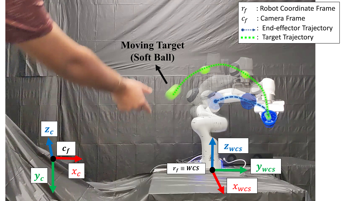
Figure 2: Hardware Platform for demonstrations. World Coordinate System Frame $WCS$ to be coincident with Robot Base Frame $r_{f}$. In Camera Frame $c_{f}$, $Z_{c}$ points inwards to frame plane and $x_{wcs}$ points outwards. [Camera not visible here]

IV System Overview

IV-A Data Accumulation Process and Research Platform

In order to build the low-dimensional manifold representation, we accumulated the dataset through using the simulation model of 7-DoFs Franka Emika Panda robotic arm inside simulation platform Robotics Toolbox (RTB) for Python[26]. Each sample of high-dimensional data contains in total $18$ numerical floating values. – $7$ joint angles $\{\theta_{i}\}_{i=0,..,6}$, $7$ pose variables of end-effector containing pose coordinates and quaternion orientations in $\mathbb{R}^{3}\times\mathcal{S}^{3}$ space, location of point obstacle $\{x,y,z\}_{o}$ and collision flag $\mathbb{I}_{F}$. We sent random but valid control signals to the simulation model with a view to reducing any bias in our dataset and introducing maximum variances in our data accumulation process. The obstacle location has been randomized periodically to maximize numbers of “collision and collision-free” samples. To perform real-hardware demonstrations, we utilized here the same 7-DoF Franka Emika Panda robotic manipulator as shown in Fig.2. The base link of the robot arm is fixed on the table top. Our object tracking and pose estimation algorithm, and adaptive trajectory planning pipeline runs on QUAD GPU server equipped with Intel Core-i9-9820X processor through straightforward Python implementation. For obstacle detection and localizing dynamic target in $\mathbb{R}^{3}$ space, we incorporated here Intel RealSense Depth Camera D435i and extracted the depth information to obtain coordinates $\{x,y,z\}_{target}$ in 3D camera coordinate frame. We also tracked the current obstacle location through depth sensing and extracted the geometry of the obstacle with a safety barrier around it. Instantly, we transformed this location into the robot’s coordinate system to catch the thrown target smoothly and timely. These continuous transformations and feedbacks from depth sensing expedited the optimum routing on the $\mathbb{R}^{2}$ manifold graph for parallel smooth execution of obstacle avoidance and target reach task. To facilitate low-latency data communication between controller and Franka Controller Interface, we have designed the whole system inside Robot Operating System (ROS) through using the Franka Integrated Library – libfranka and Franka ROS.

IV-B Data Representation and Experimentation Process

We have transformed the high-dimensional samples into low-dimensional latent space representation of $\mathbb{R}^{2}$ space in form of topological manifold. A densely connected network was formed using the learned 2D manifold representation. Shortest path from any node of this network to a target node has been formed through applying a well-known shortest path algorithm titled as Dijkstra’s algorithm. We directly sent $\Theta_{i}$–a vector of 7 joint angles for controlling the robotic arm in real-time. This control sequence was formed by detecting the shortest path from present vertice to target vertice. To cover paramount space in manipulator’s workspace, we gathered total 100k samples in our dataset for building the network. We emphasized here to collect adequate collision samples to have a safer elementary trajectory required while reaching the target location. Here, the target location is defined as the EKF predicted position in $\mathbb{R}^{3}$. To simplify object detection process and distinguish between obstacle geometry and target location, color filtering based detection has been largely used in our implementation process. In future, we plan to replace the detection block with deep-learning based varying object detection techniques for more scalable applications. However, we implemented here GJK algorithm for proximal distance detection[27] between robot’s collision mesh and current obstacle’s 3D geometry. Our variational auto-encoding (VDAE) model is implemented through Pytorch [28]. The autoencoding model simultaneously facilitates the two-way mapping between high-dimensional state space sample and low-dimensional manifold representation which inherently accelerates both shortest path routing on the manifold network and robot’s control in joint-space.

V Results Analysis

Our experiments seek to investigate the following:

1. Can we build a manifold in $\mathbb{R}^{2}$ space while keeping disparity between safe and colliding samples?

2. Can we concurrently localize the thrown object through image based visual servoing on consecutive frames and robustly predict the future position using EKF?

3. Can our proposed approach assure that the robotic entity can smoothly be able to dodge obstacles while reaching a target location through graph routing mechanisms?

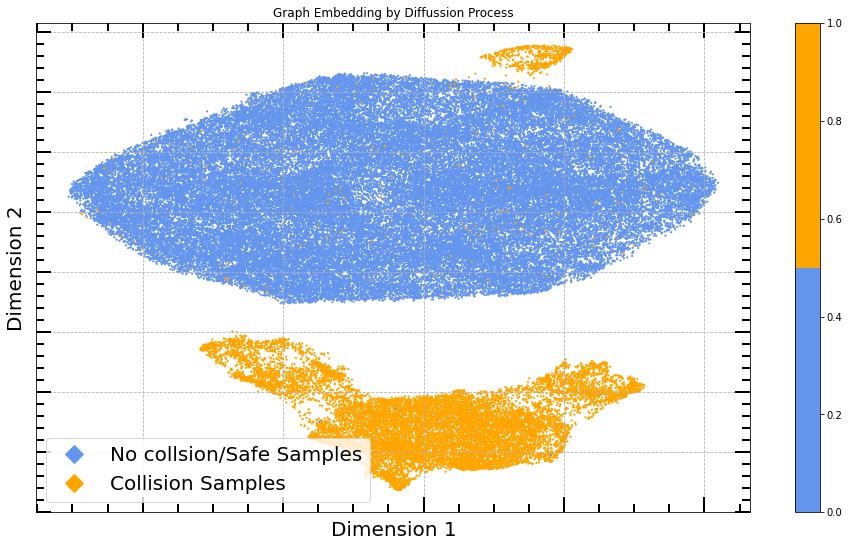
Figure 3: Diffusion Map based Low-dimensional Representation Clustered into safe and unsafe samples

V-A Topological Manifold Representation and Efficient Routing Over Manifold Network

From high-dimensional input samples of $18$ numeric values, we simply turned the representation into a geometric manifold embedded in $\mathbb{R}^{2}$ space. Through introducing the diffusion map based manifold learning, we confirmed here that proximal points in robot’s workspace would be grouped in closer neighborhood inside our low-dimensional $\mathbb{R}^{2}$-space as diffusion map always preserves the intrinsic geometric properties of our robot’s dataset inside low-dimensional space[13]. Through iterative diffusion process until convergence, the probability of motion planning through closest way-points in robot’s joint-space enhanced and smoother trajectory execution was ensured from our proposed approach while traversing towards target location and avoiding dynamic obstacles. Also as shown in Fig.3, the low-dimensional representation could be segregated between two binary labels of “collision-free/safe” samples and “colliding” samples.

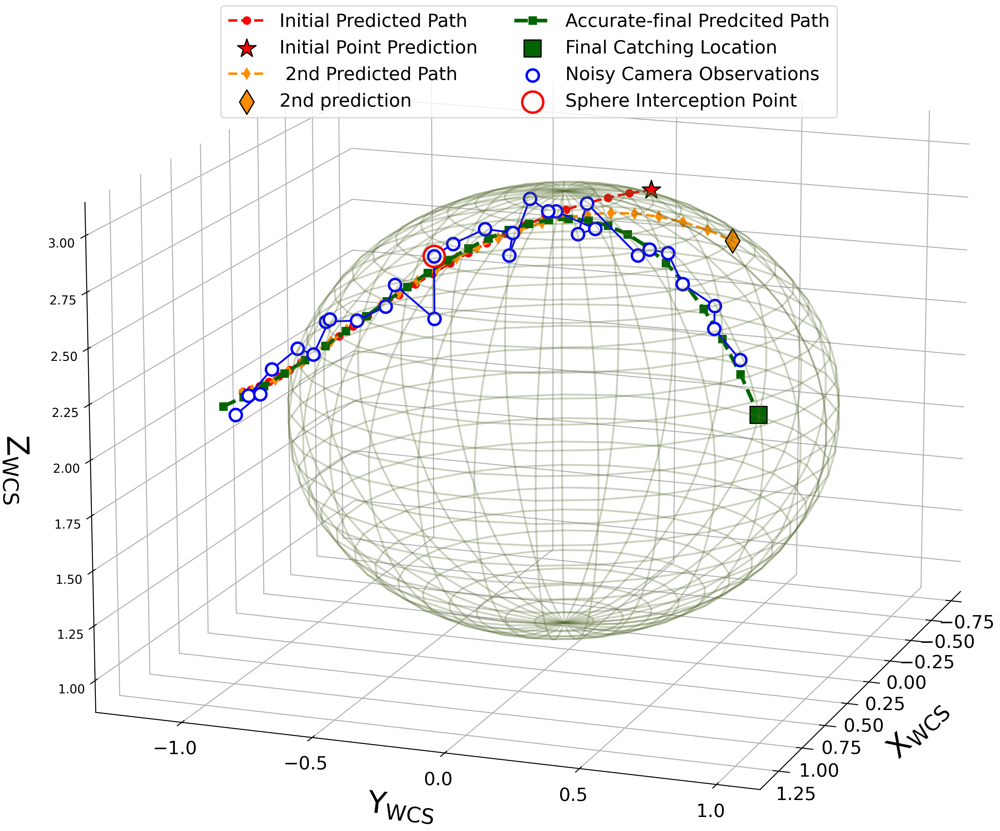
Figure 4: EKF Based Prediction Model for Estimating the Target Location

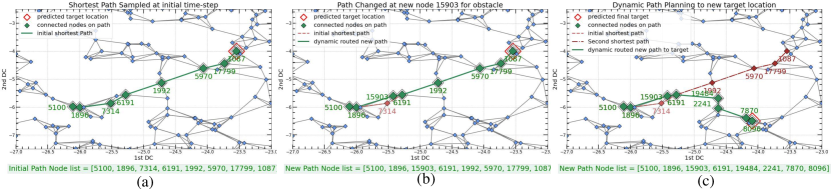
Figure 5: Dynamic Routing on the Graph (a) Initial Route to 1st predicted location, (b) New Path to avoid Obstacles, (c) Updated and accurate target location to new node, dynamic real-time path revising to catch target.

With this 2D low-dimensional manifold data, we constructed a densely connected graph $\mathcal{G}=(V,E)$ where vertices $V$ represent the safe samples and edges $E$ are the connecting links between closest manifold points. By using an unsupervised K-Nearest Neighbor algorithm[29] on the safe coded manifold points, we searched for the neighboring family of nodes of each node and connected them through connecting edges which eases any shortest path routing algorithm to create a route between any two nodes on low-dimensional manifold space. Since, the closest points in robot’s workspace were directly mapped to be in close proximity in the manifold space and high probable path to traverse existed between nodes, shortest path sampling algorithm such as Dijkstra’s algorithm expedited acquiring an optimum path and, in turn, robot controller took minimal time to reach the target location. Moreover, this network of manifold points were created by encompassing only the safe samples excluding the colliding samples. So, we could easily assume that the elementary sampled route to the target node is a safe trajectory to follow. Through dynamic routing, we retreated from this initially planned path and rerouted for more compatible motion execution if any unprecedented occlusion blocked the initial path or estimated target location got upgraded/corrected (shown in Fig.5).

V-B Object Localization and Real-time Adjustment of Routes to Target Location

We emphasized on learning two robotic skills in parallel while exploiting a unified 2D network built on low-dimensional manifold representation. In addition to developing a real-time obstacle avoidance scheme by revising its elementary planned trajectory, our principal target was to introduce a dynamic reach task for intercepting or catching any dynamically moving object. We replicated the object interception task here by throwing a ball towards the accessible work-space around the robotic arm. Whenever the ball intercepts with an artificially placed sphere around the robotic arm as shown in Fig.4, we initialized our EKF based target tracking for predicting the future position of the ball with the stored 3D location data of the thrown object extracted from depth camera. As soon as the object pose estimation block generated a future 3D location $\{x,y,z\}_{pred}$ ,we instantly queried the index, $i_{closest}$ of the closest pose of end-effector $\{x,y,z\}_{ee}^{i_{closest}}$ to $\{x,y,z\}_{pred}$ from our stored dataset. Since, the manifold points were also labelled with same index to remove mapping discrepancy and ensure one-to-one mapping, we could initialize the robot’s motion through traversing the shortest path from present vertice to target vertice,$V^{i_{closest}}_{tar}$. In order to minimize latency regarding index search, we created k-dimensional tree of end-effector’s pose using SciPy[30] library for quick nearest neighbor lookup and robot controller sent the sequence of joint vectors following the planned shortest path.

The principal goal of our study is to concurrently revise the elementary projected path over the 2D network whenever the present path is occluded by any obstacle or the predicted pose of the moving object is upgraded. With more data accumulation of the ball movement in $\mathbb{R}^{3}$ space, we performed multiple times the estimation for the 3D location of the thrown ball. In our all experiments, performing estimation in two-fold steps showed highly accurate prediction and our robotic manipulator was able to catch the ball in real-time as shown in Fig.2. Since, the projected target location got updated through multi-fold estimation steps, our dynamic planning algorithm instantly interrupts the previous trajectory execution of robotic arm and upgrades the route by forming new shortest connections from current node to the new target based on optimum path routing on our fully connected graph as shown in Fig.5(c). The fully connected network effortlessly enabled our robot controller to dynamically adjust its motion planning in real-time to catch any moving object within shortest possible time.

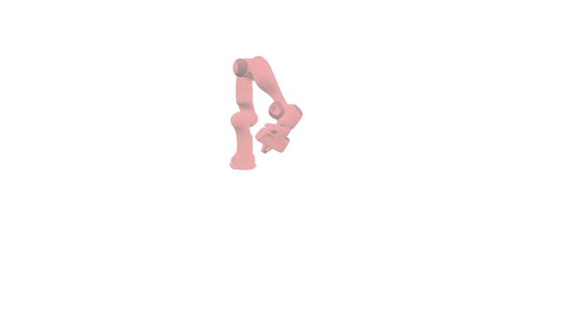
Figure 6: (a) Initial Configuration, (b)-(c) Robot initializes to move to the predicted location, (d) Robot reroutes through new path over the red obstacles, (in red shaded – collision with obstacles due to non-adaptive planning), (e)-(f) Robot catches the thrown ball at the target location

V-C Avoiding Obstacles in Real-Time While Accomplishing the Reach Task

Additionally, we aimed to get fully benefited from our fully connected manifold network for learning multiple robotic motion skills based on this common framework. While reaching a dynamically changing target location, the robotic arm can catastrophically collide with any obstacles placed in between the executing trajectory. To address such learning challenges, we again exploited our learned fully connected network of manifold data structure. Our data-driven planning methods assisted to re-plan any motion while skillfully avoiding any obstacles perturbing the present trajectory of the robotic arm. As shown in Fig.5(b), our algorithm instantly retreated from following the initial route and sampled a new path to reach the thrown ball at the predicted location. Since, we constructed a fully connected nearest neighbor network, we assured that there exists multiple paths to reach a target node from an intermediate node where the robot’s motion got suspended due to upcoming collisions. In Fig.6, we have added snapshots from the RTB simulation model showcasing how the robotic arm dodges the obstacles and reroutes through a new path to catch the moving target location in real-time. In Fig.7, we showed the evolution of end-effector position in $\mathbb{R}^{3}$ space.

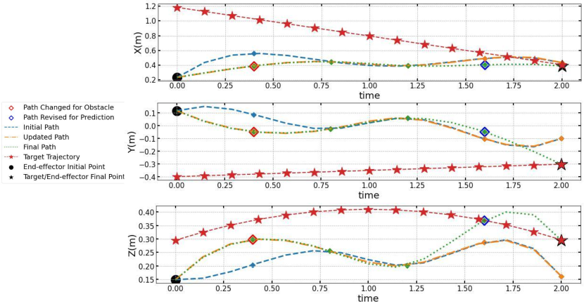
Figure 7: End-effector trajectory update sequence in $\mathbb{R}^{3}$ space with time for avoiding obstacle and catching the target with revised target pose estimation

Distance measurement API of RTB has been upgraded with the GJK algorithm[27] for calculating the proximity among 3D meshes. This algorithm produced a negative feedback when robotic arm’s collision meshes reached very close to the 3D geometry of the obstacles. In real hardware setup, we tracked the obstacles in consecutive RGB camera frames by applying color filtering through HSV color model and tracked the spatial positions of random obstacles through depth information extracted from Realsense depth camera. After successful extraction of depth values, we transported the 3D coordinate values with safety barrier around the obstacles to the learning controller for quantifying proximity distance between collision meshes of the robotic arm and 3D geometry of the obstacles. If there occurs any probability of collision, the algorithm replans for a new shortest and safest path to reach the target location position.

VI Conclusion

We presented a unified framework to let a robotic arm capture a flying object while dodging fast-moving obstacles using only depth camera sensing. Our algorithm combines three theoretical algorithm modules, namely topological manifold learning through diffusion map, variational autoencoding for high-dimensional data reconstruction, and graph traversing for intercepting the predicted target location. Besides, we incorporated here also EKF for dynamic object localization and 3D coordinate estimation. The key strength of our proposed methodology is that, for a given robotic manipulator, once our embedding manifold is learned, the robotic arm can avoid any number of 3D obstacles with arbitrary trajectories while catching a flying object, therefore versatile for fast-changing environments.

References

- [1] D. Falanga, S. Kim, and D. Scaramuzza, “How fast is too fast? the role of perception latency in high-speed sense and avoid,” IEEE Robotics and Automation Letters, vol. 4, no. 2, pp. 1884–1891, 2019.
- [2] R. R. Coifman and S. Lafon, “Diffusion maps,” Applied and computational harmonic analysis, vol. 21, no. 1, pp. 5–30, 2006.
- [3] D. Carneiro, F. Silva, and P. Georgieva, “Robot anticipation learning system for ball catching,” Robotics, vol. 10, no. 4, 2021. [Online]. Available: https://www.mdpi.com/2218-6581/10/4/113
- [4] S. Kim, A. Shukla, and A. Billard, “Catching objects in flight,” IEEE Transactions on Robotics, vol. 30, no. 5, pp. 1049–1065, 2014.
- [5] A. A. Oliva, E. Aertbeliën, J. De Schutter, P. R. Giordano, and F. Chaumette, “Towards dynamic visual servoing for interaction control and moving targets,” in 2022 International Conference on Robotics and Automation (ICRA), 2022, pp. 150–156.
- [6] S. M. Khansari-Zadeh and A. Billard, “A dynamical system approach to realtime obstacle avoidance,” Autonomous Robots, vol. 32, no. 4, pp. 433–454, 2012.
- [7] X. Cheng and S. Liu, “Dynamic obstacle avoidance algorithm for robot arm based on deep reinforcement learning,” in 2022 IEEE 11th Data Driven Control and Learning Systems Conference (DDCLS), 2022, pp. 1136–1141.
- [8] A. Dastider, S. J. A. Raza, and M. Lin, “Learning adaptive control in dynamic environments using reproducing kernel priors with bayesian policy gradients,” in Proceedings of the 37th ACM/SIGAPP Symposium on Applied Computing, ser. SAC ’22. New York, NY, USA: Association for Computing Machinery, 2022, p. 748–757. [Online]. Available: https://doi.org/10.1145/3477314.3507091
- [9] A. Zakhar’eva, A. S. Matveev, M. Hoy, and A. V. Savkin, “A strategy for target capturing with collision avoidance for non-holonomic robots with sector vision and range-only measurements,” in 2012 IEEE International Conference on Control Applications, 2012, pp. 1503–1508.
- [10] B. Ichter and M. Pavone, “Robot motion planning in learned latent spaces,” IEEE Robotics and Automation Letters, vol. 4, no. 3, pp. 2407–2414, 2019.
- [11] H. B. Mohammadi, S. Hauberg, G. Arvanitidis, G. Neumann, and L. D. Rozo, “Learning riemannian manifolds for geodesic motion skills,” in Robotics: Science and Systems, 2021. [Online]. Available: https://doi.org/10.15607/RSS.2021.XVII.082
- [12] R. Coifman, S. Lafon, A. Lee, M. Maggioni, B. Nadler, F. Warner, and S. Zucker, “Geometric diffusions as a tool for harmonic analysis and structure definition of data: Diffusion maps,” Proceedings of the National Academy of Sciences of the United States of America, vol. 102, pp. 7426–31, 06 2005.
- [13] J. De la Porte, B. Herbst, W. Hereman, and S. Van Der Walt, “An introduction to diffusion maps,” in Proceedings of the 19th symposium of the pattern recognition association of South Africa (PRASA 2008), Cape Town, South Africa, 2008, pp. 15–25.
- [14] D. P. Kingma and M. Welling, “Auto-encoding variational bayes,” 2014.
- [15] J. Lucas, G. Tucker, R. B. Grosse, and M. Norouzi, “Understanding posterior collapse in generative latent variable models,” in DGS@ICLR, 2019.
- [16] H. Li, O. Lindenbaum, X. Cheng, and A. Cloninger, “Variational diffusion autoencoders with random walk sampling,” in ECCV, 2020.
- [17] U. Shaham, K. Stanton, H. Li, B. Nadler, R. Basri, and Y. Kluger, “SpectralNet: Spectral Clustering using Deep Neural Networks,” arXiv e-prints, p. arXiv:1801.01587, Jan. 2018.
- [18] Y. F. Chen, S.-Y. Liu, M. Liu, J. Miller, and J. P. How, “Motion planning with diffusion maps,” in 2016 IEEE/RSJ International Conference on Intelligent Robots and Systems (IROS), 2016, pp. 1423–1430.
- [19] S. Hong, J. Lu, and D. P. Filev, “Dynamic diffusion maps-based path planning for real-time collision avoidance of mobile robots,” in 2018 IEEE Intelligent Vehicles Symposium (IV), 2018, pp. 2224–2229.
- [20] O. Kupervasser, H. Kutomanov, M. Mushaelov, and R. Yavich, “Using diffusion map for visual navigation of a ground robot,” Mathematics, vol. 8, no. 12, 2020. [Online]. Available: https://www.mdpi.com/2227-7390/8/12/2175
- [21] A. A. Hagberg, D. A. Schult, and P. J. Swart, “Exploring network structure, dynamics, and function using networkx,” in Proceedings of the 7th Python in Science Conference, G. Varoquaux, T. Vaught, and J. Millman, Eds., Pasadena, CA USA, 2008, pp. 11 – 15.
- [22] G. Flandin, F. Chaumette, and E. Marchand, “Eye-in-hand/eye-to-hand cooperation for visual servoing,” in Proceedings 2000 ICRA. Millennium Conference. IEEE International Conference on Robotics and Automation. Symposia Proceedings (Cat. No.00CH37065), vol. 3, 2000, pp. 2741–2746 vol.3.
- [23] B. Espiau, F. Chaumette, and P. Rives, “A new approach to visual servoing in robotics,” IEEE Transactions on Robotics and Automation, vol. 8, no. 3, pp. 313–326, 1992.
- [24] A. De Luca, G. Oriolo, and P. R. Giordano, “On-line estimation of feature depth for image-based visual servoing schemes,” in Proceedings 2007 IEEE International Conference on Robotics and Automation, 2007, pp. 2823–2828.
- [25] S. J. Julier and J. K. Uhlmann, “New extension of the kalman filter to nonlinear systems,” in Defense, Security, and Sensing, 1997.
- [26] P. Corke and J. Haviland, “Not your grandmother’s toolbox – the robotics toolbox reinvented for python,” in 2021 IEEE International Conference on Robotics and Automation (ICRA), 2021, pp. 11 357–11 363.
- [27] A. H. Khan, S. Li, and X. Luo, “Obstacle Avoidance and Tracking Control of Redundant Robotic Manipulator: An RNN-Based Metaheuristic Approach,” IEEE Transactions on Industrial Informatics, vol. 16, no. 7, pp. 4670–4680, 2020.
- [28] A. Paszke, S. Gross, F. Massa, A. Lerer, J. Bradbury, G. Chanan, T. Killeen, Z. Lin, N. Gimelshein, L. Antiga, A. Desmaison, A. Kopf, E. Yang, Z. DeVito, M. Raison, A. Tejani, S. Chilamkurthy, B. Steiner, L. Fang, J. Bai, and S. Chintala, “Pytorch: An imperative style, high-performance deep learning library,” in Advances in Neural Information Processing Systems 32, H. Wallach, H. Larochelle, A. Beygelzimer, F. d'Alché-Buc, E. Fox, and R. Garnett, Eds. Curran Associates, Inc., 2019, pp. 8024–8035. [Online]. Available: http://papers.neurips.cc/paper/9015-pytorch-an-imperative-style-high-performance-deep-learning-library.pdf
- [29] P. Cunningham and S. J. Delany, “k-Nearest Neighbour Classifiers: 2nd Edition (with Python examples),” arXiv e-prints, p. arXiv:2004.04523, Apr. 2020.
- [30] P. Virtanen, R. Gommers, T. E. Oliphant, M. Haberland, T. Reddy, D. Cournapeau, E. Burovski, P. Peterson, W. Weckesser, J. Bright, S. J. van der Walt, M. Brett, J. Wilson, K. J. Millman, N. Mayorov, A. R. J. Nelson, E. Jones, R. Kern, E. Larson, C. J. Carey, İ. Polat, Y. Feng, E. W. Moore, J. VanderPlas, D. Laxalde, J. Perktold, R. Cimrman, I. Henriksen, E. A. Quintero, C. R. Harris, A. M. Archibald, A. H. Ribeiro, F. Pedregosa, P. van Mulbregt, and SciPy 1.0 Contributors, “SciPy 1.0: Fundamental Algorithms for Scientific Computing in Python,” Nature Methods, vol. 17, pp. 261–272, 2020.