Publication Bias in Asset Pricing Research

Abstract

Researchers are more likely to share notable findings. As a result, published findings tend to overstate the magnitude of real-world phenomena. This bias is a natural concern for asset pricing research, which has found hundreds of return predictors and little consensus on their origins.

Empirical evidence on publication bias comes from large scale meta-studies. Meta-studies of cross-sectional return predictability have settled on four stylized facts that demonstrate publication bias is not a dominant factor: (1) almost all findings can be replicated, (2) predictability persists out-of-sample, (3) empirical $t$-statistics are much larger than 2.0, and (4) predictors are weakly correlated. Each of these facts has been demonstrated in at least three meta-studies.

Empirical Bayes statistics turn these facts into publication bias corrections. Estimates from three meta-studies find that the average correction (shrinkage) accounts for only 10 to 15 percent of in-sample mean returns and that the risk of inference going in the wrong direction (the false discovery rate) is less than 10%.

Meta-studies also find that $t$-statistic hurdles exceed 3.0 in multiple testing algorithms and that returns are 30 to 50 percent weaker in alternative portfolio tests. These facts are easily misinterpreted as evidence of publication bias effects. We clarify these misinterpretations and others, including the conflating of “mostly false findings” with “many insignificant findings,” “data snooping” with “liquidity effects,” and “failed replications” with “insignificant ad-hoc trading strategies.”

Meta-studies outside of the cross-sectional literature are rare. The four facts from cross-sectional meta-studies provide a framework for future research. We illustrate with a preliminary re-examination of equity premium predictability.

JEL classification: G10, G12
Keywords: publication bias, asset pricing, multiple testing, p-hacking, replication

1 Introduction

What’s the point of publishing something if it’s not worth noting? In most forms of publishing, authors are motivated to write notable content. This motive means that seemingly-notable content is over-represented in any set of published writings, and thus any set of published writings exaggerates the truth. Scientific publishing is no exception.

Science is unique in its precise definition of notable content. Even before Fisher (1925), researchers have said a finding is notable if it is at least “5% significant” (Stigler (2008)). We refer to the bias toward statistically significant results, as well as the effects of this bias, as “publication bias.”

Publication bias may seem like a very slippery issue. But its essence is found in a simple decomposition. Reported effects (e.g. regression coefficients) are the sum of the true effect and errors:

$$\text{Reported effect}=\text{True effect}+\text{Author error}+\text{Sampling error}$$ (1)

where sampling errors are statistical noise and author errors represent non-statistical problems unrelated to economics (intentional and unintentional mistakes). In an ideal world, both errors are on average zero, so the reported effect would be equal to the true effect in expectation. But under publication bias, only large reported effects are published. This bias selects for large author errors and large sampling errors, implying

$$\mathbb{E}(\text{Reported effect}|\text{Published})>\mathbb{E}(\text{True effect}|\text{Published}),$$ (2)

that is, published reported effects are upward biased relative to the true effect. The gap between the LHS and RHS of Equation (2) measures the magnitude of publication bias.

To correct for publication bias, we just need to estimate

$$\mathbb{E}(\text{Author error}|\text{Published})+\mathbb{E}(\text{Sampling error}|\text{Published}).$$ (3)

Subtracting these error terms from $\mathbb{E}(\text{Reported effect}|\text{Published})$ leads to an unbiased estimate of the true effect conditional on publication. Meta-studies with large collections of published findings can provide estimates of these error terms.

Terms like “the multiple testing problem,” “data-snooping,” “p-hacking,” “the file drawer problem,” and “researcher degrees of freedom” fill out the details. In the end, these problems boil down to selection bias and the need to correct for Equation (3).

This article reviews research on publication bias in asset pricing. Empirical evidence is abundant in cross-sectional return predictability, so we focus our review in this sub-field. We begin with four facts that emerge from these studies (Section 2). We then describe shrinkage corrections and false discovery rate estimates, which pin down publication bias at 10% to 15% of in-sample returns (Section 3). We square these results with other facts like “anomaly decay” and clarify related misinterpretations regarding the prevalance of “false findings” in Section 4. We end by illustrating how our facts provide a framework for understanding publication bias more broadly, by examining evidence from equity premium prediction (Section 5).

Before we continue, we note that there are other forms of publication bias that we do not cover. Our notion of publication bias follows the common definition of selection for notable results (De Long and Lang (1992); Brodeur et al. (2016); Andrews and Kasy (2019); etc). But researchers may also be biased toward writing papers that confirm the existing paradigm (Kuhn (1962); Akerlof and Michaillat (2018)). To our knowledge, the only empirical evidence on this kind of publication bias in finance is Rubin and Rubin (2021), who uses a natural experiment to show that a significant share of paper citations in top tier finance journals exist to curry favor with influential scholars.

2 Four Facts about Publication Bias in the Cross-Section of Returns

Cross-sectional predictability refers to the idea that some stocks have higher average future returns than others. These differences in expected returns are typically documented by sorting stocks into portfolios based on some firm-level characteristic, and then examining the performance of going long-short the extreme portfolios. A series of meta-studies re-examine dozens, or even hundreds of published cross-sectional predictors (e.g. Green et al. (2013); McLean and Pontiff (2016); Chen and Zimmermann (2022)).

This literature finds four salient facts:

1. Almost all predictability findings can be replicated

2. Predictability persists out-of-sample

3. Empirical t-stats are much, much larger than 2.0

4. Predictors are weakly correlated

Each of these facts has been documented by at least three different meta-studies.

The importance of these facts can be seen in Equation (1). High replicability (Fact #1) rules out author error as a meaningful influence. Out-of-sample persistence (Fact #2) limits the impact of sampling error, as sampling error should vanish out-of-sample. Very large t-stats (Fact #3) also limit the impact of sampling error, as they imply sampling error is small. Weak correlations (Fact #4) show that the zoo of predictors is not redundant, and also validates assumptions used in the multiple testing statistics.

We illustrate these facts using the Chen and Zimmermann (2022) (CZ22) dataset. This dataset consists of replications of hundreds of variables that were claimed to be related to cross-sectional predictability. It includes the vast majority of predictors found in previous meta-studies (McLean and Pontiff (2016); Green et al. (2017); Hou et al. (2020)). Unlike other meta-studies, we compare our replications to hand-collected findings from the original papers. We also post data, code, and detailed documentation at https://www.openassetpricing.com/, and update these data annually, fixing errors and occasionally adding new predictors. The version used in this review is the March 2022 release, which contains 207 cross-sectional predictors published in 140 papers.

The dataset includes many portfolio implementations of these 207 predictors. For this review, we focus on raw long-short portfolios constructed following the methods in the original papers. Code to replicate the results in this review are found at https://github.com/chenandrewy/PBR.

2.1 Fact #1: Almost all predictability findings can be replicated

McLean and Pontiff (2016) and Jensen, Kelly, and Pedersen (2022) find that most of their implementations of published cross-sectional predictors are statistically significant. CZ22 go further and show that nearly all findings can be replicated. Figure 1 illustrates this result.

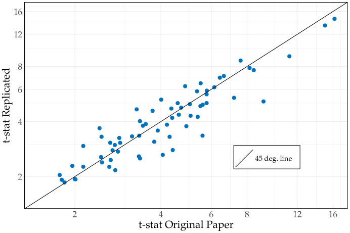
Figure 1: Replicated vs Original Paper t-stats. Each marker represents a different cross-sectional predictor from the CZ22 dataset. t-stats test the hypothesis that the mean return on a long-short strategy that trades on the predictor in the original sample period is zero. We show only predictors for which the original papers provide raw long-short t-statistics. Solid line is the 45 degree line. On average, CZ22’s replicated t-stats match the original t-stats. These replications can surely be improved with more economist-hours.

The figure plots CZ22’s replicated t-stats against t-stats hand-collected from the original papers. The markers line up nicely along the 45 degree line, showing that cross-sectional predictability can not only be replicated qualitatively, but quantitatively.

The replicated t-stats deviate somewhat from the originals. CZ22 aim to cover all predictors in four previous meta-studies, leading to a list of 319 characteristics from 153 papers. These 319 characteristics are replicated with a team of just two economists, so each replication can surely be improved with more economist-hours. But considering this limitation, the match is remarkable.

This result bounds the effects of “author error” in Equation (3). If author error was a big problem, then the markers would lie far below the 45 degree line. Instead, Figure 1 shows that author error is on average close to zero. In other words, the numbers in the original papers are a fairly unbiased estimate of what a researcher who attempts to replicate the original findings would obtain.

In contrast, Hou, Xue, and Zhang (2020) find that “most anomalies fail to replicate.” This is commonly reconciled with other meta-studies by noting that Hou et al.’s long-short strategies de-emphasize microcap stocks. However, this reconciliation is not correct. The proper reconciliation is misclassification of failed replications: only about 26% of Hou et al.’s long-short strategies were shown to be clearly statistically significant in the original papers (Chen and Zimmermann (2022); see also Jensen et al. (2022)). We discuss this and other misinterpretations in Section 4.

2.2 Fact #2: Predictability persists out-of-sample

If predictability was entirely due to publication bias, then it should vanish immediately after the original samples end. But McLean and Pontiff (2016) (MP) find nearly the opposite pattern.

MP replicate 97 published predictors and compare their returns from the original sample periods to their returns between the end of the original sample and the publication date. Returns decline by only 26%. In other words, the in-sample returns are still 74% there. A similar out-of-sample decline is documented in Jacobs and Müller (2018) and Chen and Zimmermann (2020).

Figure 2 replicates MP’s result using the CZ22 dataset. Long-short returns are scaled so that the mean in-sample return is 100 bps per month for ease of interpretation. In the first 3 years after the end of the original samples, the mean return is still 74 bps per month (vertical line). These out-of-sample periods are short, but large scale replications like MP’s still show statistical significance. This significance is seen in the bootstrapped distribution of the out-of-sample mean (grey bars). After accounting for sampling uncertainty, these out-of-sample returns are still far from zero, and quite close to in-sample returns (blue bars).

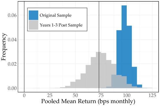
Figure 2: Predictability persists out-of-sample. Long-short returns are scaled so that the mean in-sample return is 100 bps per month for ease of interpretation. Blue shows the mean return pooled across all in-sample observations. Gray shows the pooled mean return using data from the first three years after the original samples end. Distributions indicate sampling uncertainty via cluster bootstrap, which draws all returns in the same month simultaneously. 74% of returns persist in these out-of-sample periods.

MP’s 26% decline places an upper bound on the effects of “sampling error” in Equation (3). This small decline is a tough challenge for believers in the dominance of publication bias. As argued by MP, this 26% decline is an upper bound because investors should learn from the academic publications, and may trade away (or avoid creating) the documented return patterns (see also Marquering et al. (2006)). The actual effects of sampling error may be much smaller than 26%.

Returns far from the original sample periods have a larger decay of roughly 50% (McLean and Pontiff (2016); Linnainmaa and Roberts (2018); Jacobs and Müller (2020); Jensen et al. (2022)). Since publication bias should show up immediately after the samples end, the remaining decay is due to real changes in expected returns (see Equation (1)). These changes are natural given that many, if not most of the original papers argue for mispricing-based explanations (Rosenberg et al. (1985); Jegadeesh and Titman (1993); etc). We return to this issue in Section 4.

2.3 Fact #3: Empirical t-stats are much larger than 2.0

The common story for publication bias goes something like this: even if there’s no predictability, you’ll find 5% significance if you just p-hack $1/0.05=20$ strategies. Since 5% significance corresponds to a t-stat of 2.0, this suggests it’s quite possible that t-stats near 2.0 are due to publication bias.

But the t-stats found in the literature are much larger than 2.0. Table 1 provides the details, using the distribution of t-stats found in the CZ22 data. The majority of t-stats exceed 3.0, and plenty of t-stats exceed 4.0. There are even predictors with t-stats that exceed 8.0. Similar results are found in hand-collected t-stats (Green et al. (2013); Chen and Zimmermann (2020)).

Table 1: Published t-stats are much larger than 2.0.

“Published and Replicated” are from CZ22’s replications of 207 predictors. “Systematically Data-Mined” are from Yan and Zheng (2017)’s 18,113 equal-weighed strategies mined by sorting stocks on simple functions of 240 accounting variables. The bootstrap draws de-meaned returns from the CZ22 data, with returns in the same month drawn simultaneously to control for correlations. Large t-stats are thousands of times more common than implied by the null of no predictability.

	t-stat minimum
	2.0	3.0	4.0	5.0	6.0	7.0	8.0
	(a) Number of Predictors that Meet Minimum
Published and Replicated	183	121	74	48	26	18	12
Systematically Data-Mined	5,464	2,837	1,522	832	374	185	76
	(b) Percent of Signals that Meet Minimum
Published and Replicated	88.4058	58.4541	35.7488	23.1884	12.5604	8.6957	5.7971
Systematically Data-Mined	30.1662	15.6628	8.4028	4.5934	2.0648	1.0214	0.4196
	(c) Percent of Signals Implied by Null (Significance Level)
Standard Normal	4.5500	0.2700	0.0063	0.0001	0.0000	0.0000	0.0000
Bootstrap	4.6115	0.3034	0.0107	0.0002	0.0000	0.0000	0.0000

While it would take only about $1/0.05=20$ draws to generate a t-stat greater than 2.0, it would take $1/0.000063\approx 16,000$ draws to generate just one of the 74 t-stats that exceeds 4.0. For the 26 t-stats that exceed 6.0, the significance is so strong that it can’t be seen in the table. It would take $1/0.000000002=50$ billion draws to generate just one of these t-stats. It is physically impossible that these 26 t-stats are found in the literature if there is no predictability (Chen (2021)).

These thought experiments illustrate the limits of “sampling error” in Equation (1). Sampling error can only explain t-stats that are close to the null of no predictability. t-stats far from the null, then, must be due to positive expected returns. And while publication bias may distort the magnitude of published t-stats, this distortion would have to be very extreme to account for the gap seen in Table 1. Moreover, publication bias does not distort the empirical probabilities found in atheoretical data-mining experiments (Yan and Zheng (2017); Chordia et al. (2020)). As seen in Panel (b), even atheoretical data mining generates large t-stats thousands of times too frequently to be due to luck.

Multiple testing statistics convert this intuition into publication bias corrections. Shrinkage estimates imply that sampling error in Equation (3) is only 10% to 15% of in-sample returns. False discovery rate estimates imply that the risk of expected returns being zero or negative is less than 10%. These small publication bias effects are found in models estimated by three independent meta-studies (Harvey et al. (2016); Chen and Zimmermann (2020); Jensen et al. (2022)). We explain these statistics in detail in Section 3.

In contrast, Harvey et al. (2016) famously “argue that most findings in financial economics are likely false.” Despite this language, their estimates imply a false discovery rate of less than 10% (see Section 3.3 below). This confusion is also seen in Harvey et al’s conclusion, which mixes the terms “mostly false findings” with “many insignificant findings.” It’s easy to confuse significance with truth in standard hypothesis testing (Wasserstein and Lazar (2016)). It’s even easier to mix up the language in multiple testing statistics. We discuss this issue further in Section 4.

2.4 Fact #4: Predictors are weakly correlated

A common view is that the zoo of predictors are just hacked copies of a handful of real predictors like value and momentum. But the data show the predictors are quite diverse.

Figure 3 illustrates this diversity. It shows the distribution of correlations between pairs of long-short returns in the CZ22 data. All long-short returns are signed to have positive mean returns, so highly negative correlations indicate very distinct predictors.

Figure 3: Predictors are weakly correlated. Data consists of monthly long-short returns from the CZ22 dataset. All returns are signed to have positive in-sample means. Almost all correlations are less than 0.5 and 60 principal components are required to span 90% of total variance, indicating a zoo of distinct predictors.

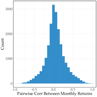
(a) Distribution of Correlations

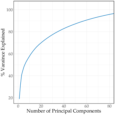
(b) Principal Component Analysis

The mean, median, and modal correlation is close to zero. Almost all correlations fall below 0.5, indicating a zoo of distinct strategies. This diversity is also seen in principal component analysis. Panel (b) shows that it takes 60 principal components to span 90% of total variance. These weak correlations have been documented in many ways and in many papers (Green et al. (2013); McLean and Pontiff (2016); Chen and Zimmermann (2020); Bessembinder et al. (2021); Chen and Zimmermann (2022)).

Weak correlations are intuitive given the publication process. Referees at top tier finance journals are notoriously skeptical. Moreover, they seem to believe in a strong factor structure in stock returns. It’s only natural that the predictors that make it through the referee process are distinct from other predictors.

Weak correlations are also important for multiple testing statistics. They imply that the small publication bias corrections found in Harvey et al. (2016) and Chen and Zimmermann (2020) are valid. We explain these estimates next.

3 Just How Large Are Publication Bias Effects in the Cross-Section?

McLean and Pontiff (2016)’s out-of-sample test (Fact # 2, Section 2.2) is a critical starting point. It means publication bias drives at most 26% of the returns reported in journals.

However, the out-of-sample periods are about four years long, leading to standard errors of around 10 percentage points. So loosely speaking, out-of-sample decay only tells us that publication bias accounts for between 0% and 46% of published returns.

Using the gap between the empirical and null t-stat distribution (Fact # 3) leads to more precise estimates. Shrinkage and false discovery rate (FDR) methods transform this gap into estimates of publication bias effects, which are valid under weak dependence (Fact # 4). Three independent meta-studies find estimates that imply publication bias effects account for 10% to 15% of in-sample performance (Harvey et al. (2016), Chen and Zimmermann (2020), Jensen et al. (2022)).

3.1 Publication Bias Corrections

Publication bias corrections can be understood in a four equation model.

Authors generates ideas for predictors. The t-stat for idea $i$ has two components:

$$t_{i} =\theta_{i}+Z_{i}$$ (4)

$$Z_{i} \sim\text{Normal}(0,1)$$ (5)

where $\theta_{i}$ is the expected return divided by the standard error and $Z_{i}$ is sampling error divided by the standard error.

$\theta_{i}$ is the key variable and has two interpretations. The first is that it’s the expected return (in units of standard errors). The second is that it’s a corrected t-statistic, since it corrects $t_{i}$ for sampling error $Z_{i}$, and thus publication bias. We’ll use both interpretations in what follows.

Since there are many ideas, $\theta_{i}$ is not a constant, but drawn from a distribution $f_{\theta}(\cdot|\sigma_{\theta})$

$$\theta_{i} \sim f_{\theta}(\cdot|\sigma_{\theta})$$ (6)

where $\sigma_{\theta}$ is a parameter vector that controls the properties of the distribution (e.g. variance). We’ll see this distribution is critical for determining publication bias corrections.

Publication bias means that observed ideas are a selected sample, given by

$$\Pr(\text{pub}_{i}|t_{i},\theta_{i}) =p(t_{i},\theta_{i}|\sigma_{\text{pub}})$$ (7)

where $\text{pub}_{i}$ indicates observation and $\sigma_{\text{pub}}$ is a parameter vector. In general, $p(t_{i},\theta_{i}|\sigma_{\text{pub}})$ is weakly increasing in both the t-stat $t_{i}$ and the underlying expected return $\theta_{i}$.

Equations (4)-(7) typically imply that published t-stats overstate expected returns:

$$\mathbb{E}(t_{i}|\text{pub}_{i};\sigma_{\theta},\sigma_{\text{pub}}) =\mathbb{E}(\theta_{i}|\text{pub}_{i};\sigma_{\theta},\sigma_{\text{pub}})+\underbrace{\mathbb{E}(Z_{i}|\text{pub}_{i};\sigma_{\theta},\sigma_{\text{pub}})}_{>0}.$$ (8)

This is the essence of publication bias. If a paper says that the sample mean return is, say, three standard errors from zero ($t_{i}=3$), the expected return is closer to zero ($\theta_{i}<3$) because positive sampling errors are selected ($\mathbb{E}(Z_{i}|\text{pub}_{i};\sigma_{\theta},\sigma_{\text{pub}})>0$). Equation (8) is very close to Equation (1), but it makes explicit the fact that many tests have been run. The many tests are embodied by $\sigma_{\theta}$, which contains information on an infinite number of tests (Equation (6)).

To correct for this bias, we just need to remove $\mathbb{E}(Z_{i}|\text{pub}_{i};\sigma_{\theta},\sigma_{\text{pub}})$. If we scale this term by the mean published t-stat, we get a “shrinkage correction”:

$$\text{Shrinkage}_{\text{pub}}\equiv\frac{\mathbb{E}(Z_{i}|\text{pub}_{i};\sigma_{\theta},\sigma_{\text{pub}})}{\mathbb{E}(t_{i}|\text{pub}_{i};\sigma_{\theta},\sigma_{\text{pub}})},$$ (9)

This says we have to shrink the mean published t-stat toward zero at a rate of $\text{Shrinkage}_{\text{pub}}$ to recover the corresponding expected return.

Shrinkage measures the average correction. The FDR measures tail risk:

$$\text{FDR}_{\text{pub}}=\Pr(\theta_{i}\leq 0|\text{pub}_{i};\sigma_{\theta},\sigma_{\text{pub}})$$ (10)

That is, if we define ideas with zero or negative expected returns as “false predictors” and published predictors as “discoveries,” then the FDR is the risk of discovering a false predictor.

There are many variations of shrinkage and the FDR. Instead of conditioning on publication, these objects can condition on some other subset of tests (e.g. $2<t_{i}\leq 3$). The FDR can also be defined using $\theta_{i}=0$ instead of $\theta_{i}\leq 0$, or using the FDR definitions from Benjamini and Hochberg (1995) or Storey (2003). With many predictors and a non-trivial share of true predictors, these differences are more technical than meaningful (Benjamini (2008)). In the end, shrinkage measures the average correction and the FDR measures tail risk.

Using Equation (8) to define corrections for publication bias is explicitly described in Chen and Zimmermann (2020) and is implicitly used throughout the meta-study literature on the cross-section of returns (McLean and Pontiff (2016), Jensen et al. (2022); Harvey et al. (2016)). This notion of a false discovery is consistent with the statistics literature (Benjamini and Hochberg (1995); Storey (2003)), but the recent finance literature uses looser language (Section 4).

3.2 Publication Bias Corrections Are Roughly 10% of In-Sample Returns

The simplest estimates come from assuming normal (standardized) expected returns that are orthogonal to sampling error

$$\theta_{i} \sim\text{Normal}(0,\sigma_{\theta}^{2})$$ (11)

$$\text{Cov}(\theta_{i},Z_{i}) =0$$ (12)

and a clean hurdle for publication

$$\Pr(\text{pub}_{i}|t_{i},\theta_{i})=\begin{cases}\bar{p},\quad t_{i}>2\\ 0,\quad\text{otherwise}.\end{cases}$$ (13)

This model is a slight generalization of Appendix A.2 of Chen and Zimmermann (2020).

The model is also conservative. Equation (11) assumes, pessimistically, that the ideas of finance scholars have expected returns that are on average zero. In the real world, the intuition and theory of finance scholars should on average produce positive expected returns. Similarly, Equation (13) assumes $\text{pub}_{i}$ is only related to $\theta_{i}$ through $t_{i}$—a kind of pure data-mining setting. In the reality, publication should also be positively related to $\theta_{i}$ through the underlying quality of the paper (Card and DellaVigna (2020)).

These assumptions imply that $t_{i}\sim\text{Normal}(0,\sigma_{\theta}^{2}+1)$ and that $t_{i}|\text{pub}_{i}$ is just $t_{i}$ truncated from below at 2. $\bar{p}$ drops out in the distribution of $t_{i}|\text{pub}_{i}$, so the model just has a single meaningful parameter, the variance of expected returns $\sigma_{\theta}^{2}$ (in units of standard errors).

$\sigma_{\theta}^{2}$ can be estimated by GMM or quasi maximum likelihood. While $t_{i}$ and $t_{j}$ are not independent, Fact #4 (Section 2.4) shows the correlations are mild and center around zero, so standard econometric methods are valid (Wooldridge (1994)). Estimation is illustrated in Figure 4. For $\sigma_{\theta}^{2}=0$, the model (dotted line) is very far from the data. Increasing $\sigma_{\theta}$ to 1.5 (dashed line) improves the fit, but the gap is still large. $\sigma_{\theta}\approx 3.0$ (solid line) fills the gap, fitting many moments seen in this figure.

Figure 4: Expected returns fill the gap. Bars are $t_{i}$ from the CZ22 dataset. Lines are a simple model (Equations (4)-(5) and (11)-(13)) where the key parameter is $\sigma_{\theta}^{2}=\text{Var}(\theta_{i})$, the variance of expected returns (in units of standard errors). The null of no predictability $\sigma_{\theta}=0$ is very far from the data. $\sigma_{\theta}\approx 3$ is required to fill the gap, implying that expected returns three standard errors from zero are common.

What does $\hat{\sigma}_{\theta}\approx 3.0$ mean? It means that finance researchers’ ideas commonly have expected returns three standard errors away from zero. Since the average standard error is about $20$ bps per month (Chen and Zimmermann (2020)), this means that it’s easy to find a predictor with a true expected return of $20\times 3=60$ bps per month. It also means shrinkage and FDR estimates are small.

Figure 5 illustrates the implied shrinkage. We simulate $\theta_{i}$ and $t_{i}$ using $\hat{\sigma}_{\theta}=3.0$. We then keep only published ideas using Equation (13), and plot the distribution of $\theta_{i}|\text{pub}_{i}$ (blue). These standardized expected returns (alternatively, corrected t-stats) are not far from the published t-stats (grey), showing that publication bias is small. The small difference between the means of these distributions (dashed lines) shows that $\text{Shrinkage}_{\text{pub}}$ is only 10%.

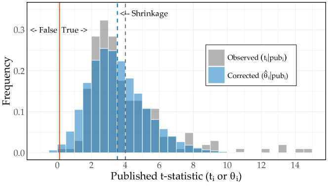
Figure 5: Simple Shrinkage and FDR Estimates. Plot compares the distribution of t-stats (grey) and corrected t-stats (blue) conditional on publication, as implied by the simple model (Equations (4)-(5) and (11)-(13)). The model uses $\hat{\sigma}_{\theta}^{2}=\widehat{\text{Var}}(\theta_{i})=3.0^{2}$ (Figure 4). Dashed lines show the means of each distribution. The distance between these lines implies $\text{Shinkage}_{\text{pub}}$ = 10%. $\text{FDR}_{\text{pub}}=0.4\%$ is the tiny mass of corrected t-stats to the left of the solid line.

Bayesian reasoning provides the intuition:

$$\mathbb{E}(\theta_{i}|t_{i},\text{pub}_{i},\sigma_{\theta}) =\mathbb{E}(\theta_{i}|t_{i},\sigma_{\theta})=\left(1-\frac{1}{1+\sigma_{\theta}^{2}}\right)t_{i}.$$ (14)

The first equality comes from assuming $\text{pub}_{i}$ provides no information about $\theta_{i}$ over-and-above $t_{i}$ (Equation (13)), and is sometimes referred to as the “immunity” of Bayes rule to selection bias (Efron (2011); Chen and Zimmermann (2020)). The second equality uses standard bi-variate normal formulas.

Equation (14) says we should shrink t-stats toward our “prior,” embodied in $\sigma_{\theta}$. A small $\sigma_{\theta}$ is a strong “prior” that the expected return is zero, in which case shrinkage is large. These “priors” are not subjective beliefs of Bayesian statistics, but parameters estimated from empirical data. For this reason, Equation (14) is often referred to as “empirical Bayes” shrinkage. Plugging in our estimate of $\hat{\sigma}_{\theta}=3$, we have

$$\mathbb{E}(\theta_{i}|t_{i},\text{pub}_{i},\hat{\sigma}_{\theta}) =\left(1-\frac{1}{10}\right)t_{i}.$$ (16)

That is, published t-stats are overstated by just 10%.

$\text{FDR}_{\text{pub}}$ is seen in the left tail of Figure 5. Only a tiny mass of the corrected t-stats fall to the left of the solid line, corresponding to $\text{FDR}_{\text{pub}}=0.4\%$. The intuition once again comes from Bayes rule:

$$\text{FDR}_{\text{pub}} =\frac{\Pr(t_{i}>2|\theta_{i}\leq 0,\sigma_{\theta})}{\Pr(t_{i}>2|\sigma_{\theta})}\Pr(\theta_{i}\leq 0|\sigma_{\theta})$$ (17)

$$\leq\frac{\Pr(t_{i}>2|\theta_{i}=0)}{\Pr(t_{i}>2|\sigma_{\theta})}\Pr(\theta_{i}\leq 0)|\sigma_{\theta}).$$ (18)

where the second line comes from the fact that large t-stats are even less likely if $\theta_{i}$ is strictly less than zero. This expression says we update our “prior” about $i$ being false ($\Pr(\theta_{i}\leq 0)|\sigma_{\theta})$) by comparing the null likelihood $\Pr(t_{i}>2|\theta_{i}=0)$ to the data $\Pr(t_{i}>2|\sigma_{\theta})$. If the null and data are far apart, this fraction is small, and $\text{FDR}_{\text{pub}}$ is small. Plugging in our estimated $\theta_{i}\sim\text{Normal}(0,3^{2})$ and $t_{i}\sim\text{Normal}(0,10)$:

$$\text{FDR}_{\text{pub}} \leq\frac{0.025}{0.25}(0.5)=4.8\%.$$ (19)

That is, the risk of a published predictor having zero or negative returns is at most 4.8%.

3.3 Publication Bias Estimates Implied by Meta-Studies Are Also Small

Harvey, Liu, and Zhu (2016); Chen and Zimmermann (2020); and Jensen, Kelly, and Pedersen (2022) estimate the distribution of corrected t-stats ($\theta_{i}$) using methods that are much more sophisticated than those in Section 3.2. Nevertheless, the resulting distributions are quite similar: all find that expected returns three standard errors away from zero are common.

The distributions of $\theta_{i}$ from these papers are shown in Figure 6. These papers differ in their modeling of null predictors: Harvey et al. (2016) put all null predictors into the mass near zero, while Chen and Zimmermann (2020) and Jensen et al. (2022) allow for negative $\theta_{i}$. This results in differences for $\theta_{i}\leq 0$, but to the right of zero the distributions are quite similar. They all imply that predictors with $\theta_{i}>0$ on average have $\theta_{i}\approx 2$, not far from our one-parameter estimate.

Figure 6: Distribution of Corrected t-stats ($\theta_{i}$) from the Literature. Harvey, Liu, and Zhu (2016) uses their baseline SMM estimate (their Table 5, Panel A, $\rho=0.2$). Chen and Zimmermann (2020) uses their baseline (Table 3, “All”). Jensen, Kelly, and Pedersen (2022) uses their baseline publication bias adjustment (Figure 9, $\tau_{c}=0.29\%$). “Simple Normal” uses Section 3.2 (based on Chen and Zimmermann (2020)’s appendix). The literature differs in the modeling of the null ($\theta_{i}\leq 0$) but for $\theta_{i}>0$ the distributions are similar to the simple normal model (Figure 4). All find that expected returns three standard errors from zero are common.

This commonality is striking because the estimates are made by independent teams. The teams differ in members, data sources, publication modeling, expected return modeling, and estimation method. Some t-stats were hand-collected, while others were replicated. Some modeled Equation (7) explicitly, while others used informal adjustments. Expected returns were modeled as mixtures, t-distributed, or hierarchical normal. Even the estimation differed, from SMM to (quasi) maximum likelihood to full maximum likelihood. All of these different methods lead to similar inferences about the right tail of $\theta_{i}$. Comparable estimates are also found in Chinco, Neuhierl, and Weber (2021), using yet another approach.

The common tail leads to similar shrinkage and $\text{FDR}_{\text{pub}}$ estimates. Chen and Zimmermann (2020) reports $\text{Shrinkage}_{\text{pub}}$ estimates between 8% and 17% across a wide range of models. In the working paper version (Chen and Zimmermann (2018)) we also report $\text{FDR}_{\text{pub}}\approx 1\%$. Jensen et al. (2022) report shrinkage of 10% and an $\text{FDR}_{\text{pub}}\approx 0.1\%$ before adjusting for publication bias, but adjusting for publication bias has only minor effects. A simple calculation shows their publication bias adjusted shrinkage is around 13%.

Harvey et al. (2016) don’t report shrinkage or $\text{FDR}_{\text{pub}}$, but these corrections can be easily calculated by Monte Carlo. Figure 7 illustrates the calculation. We simulate Harvey et al. (2016)’s baseline model and plot the distribution of published corrected t-stats $\theta_{i}|\text{pub}_{i}$. A minor complication is that Harvey et al. (2016) assume publication depends on $|t_{i}|$ rather than $t_{i}$. Nevertheless, the corrected t-stats (blue) are close to their observed counterparts $|t_{i}||\text{pub}_{i}$ (grey). $\text{Shrinkage}_{\text{pub}}=13\%$ and $\text{FDR}_{\text{pub}}=6.3\%$.

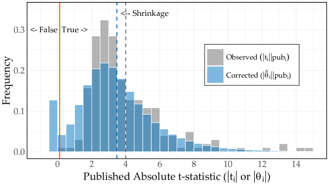
Figure 7: Shrinkage and FDR Estimates in Harvey et al. (2016). Plot compares the distribution of published t-stats (grey) to the distribution of standardized expected returns (blue) implied by Harvey et al. (2016)’s baseline estimate (Table 5, Panel A, $\rho=0.2$). Dashed lines show the means of each distribution. The distance between these lines implies $\text{Shrinkage}_{\text{pub}}$ = 13%. $\text{FDR}_{\text{pub}}=6.3\%$ is the mass of expected returns to the left of the solid line. These corrections are similar to the simple model (Figure 5) because the right tail of $\theta_{i}$ is similar (Figure 6).

3.4 Model-Free Supporting Evidence

Harvey et al. (2016), Chen and Zimmermann (2020), and Jensen et al. (2022) use models to extrapolate the distribution of $\theta_{i}$ from published results. These models all lead to similar bias corrections, but one would like to see model-free evidence.

Model free evidence comes from the data-mining experiments of Yan and Zheng (2017) and Chordia, Goyal, and Saretto (2020). These papers systematically mine Compustat accounting data for signals to trade on. Compustat contains more than 200 accounting variables, and since signals typically combine at least two variables, it’s quite easy to generate 200 choose 2 $\approx$ 20,000 signals. Yan and Zheng generate 18,000 signals, while Chordia et al. generate 2 million. By comparing the t-stats from these signals to the null distribution, one can get a sense of the distribution of $\theta_{i}$ from pure data mining.

The distribution of $|t_{i}|$ found in the Yan and Zheng (2017) data is shown in Table 1 (back in Section 2.3). The distribution is very far from the null. 30% of $|t_{i}|$ exceed 2.0, six times the null probability of 5%. The distance becomes extremely pronounced further in the tail. 4.5934% of $|t_{i}|$ exceed 5.0, 20,000 times more common than the null probability of 0.0002%. The distribution found in Chordia et al. (2020) is not quite so dispersed because they focus on value-weighting. Nevertheless, Chordia et al. (2020) find that 10 to 20 percent of $|t_{i}|$ exceed 2.0, at least double the 5% found under the null. Neither paper finds a huge spike in t-stats near zero, suggesting that the smooth modeling of $\theta_{i}$ in Chen and Zimmermann (2020) and Jensen et al. (2022) is more appropriate than the Dirac delta mixture in Harvey et al. (2016) (Figure 6).

4 Interpreting and Mis-Interpreting Meta-Studies

Facts 1-3 (Section 2) are straightforward to interpret. Each fact measures either the author error or the sampling error in published studies. Both types of error are small, even if data-mining is widespread (Section 3).

Other facts from meta-studies are more tricky. Returns are about 50% weaker far from the original samples. Returns are about 30% weaker after liquidity adjustments. Many predictors are insignificant under some multiple testing methods.

It tempting to interpret these negative results as evidence of publication bias (i.e. data snooping, p-hacking, etc). But since Facts 1-3 limit the role of author error and sampling error, these findings of return decay largely document variation in expected returns (Equation (1)). This variation is important, but it does not measure publication bias effects.

The finding that many predictors are insignificant in multiple testing methods is not like the others. It is fragile and depends entirely on highly conservative hypothesis tests.

4.1 Many Predictors Are Insignificant Under Some Many-Hypothesis Methods

Figure 8 illustrates this finding by simulating Harvey et al. (2016)’s baseline estimate. It plots the standardized expected return $\theta_{i}$ against the absolute t-stat $|t_{i}|$, with each marker representing one predictor. Harvey et al. (2016)’s model assumes $\theta_{i}=0$ for all false predictors, which makes them hard to see in a scatterplot. We add $\text{Normal}(0,0.1)$ noise to these markers for ease of viewing.

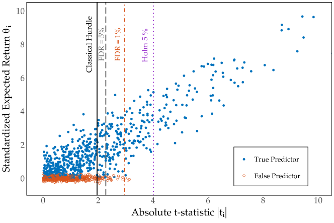
Figure 8: Multiple Testing vs Conservatism in Harvey, Liu, and Zhu (2016). We simulate predictors following Harvey et al. (2016)’s baseline estimate (Table 5, Panel A, $\rho=0.2$). $\text{Normal}(0,0.1)$ noise is added to the false predictors for ease of viewing. We plot a random sample of 1,172 total predictors, which implies roughly 300 predictors with $|t_{i}|>1.96$. The classical 1.96 hurdle implies an FDR of 8.8% (share of hollow markers to the right of solid line). FDR = 5% requires raising the hurdle a bit, to 2.3 (dashed line). Harvey et al. (2016) recommend a more a conservative FDR = 1% (dotted line), or using the Holm (1979) algorithm at FWER $\leq$ 5% (dotted line), among other more conservative methods. Holm is computed using the 1,383 predictors shown. The significant raising of hurdles is due to conservatism, not multiple testing effects.

The classical hurdle of 1.96 implies an FDR of only 8.8%, as seen in the small share of false predictors (empty markers) to the right of $|t_{i}|=1.96$. To achieve an FDR of 5%, the hurdle should be raised slightly, to 2.3 (dashed line). Given the uncertainty in these estimates, it is reasonable to think that the classical hurdle need not be raised at all. One would like to examine standard errors here, but Harvey et al. (2016) do not report them.

FDR = 5% is not only a natural counterpart to the Fisher (1925)’s 5%. It is also a popular choice in fields from genomics to functional imaging (Benjamini (2020)). But Harvey et al. (2016) focus on FDR = 1%, five times more stringent than the traditional level. This choice calls for raising the hurdle substantially, to 3.0 (dash-dot line), leading to many insignificant findings to the right of 1.96. However, 81% of these insignificant findings are true predictors and have an average expected return 1.6 standard errors from zero. These insignificant findings say little about publication bias. They can only be interpreted as increased conservatism.

Conservatism drives other calls for raising the classical hurdle. Harvey et al. (2016) also justify raising the hurdle using Theorem 1.3 of Benjamini and Yekutieli (2001). This method is thought by the statistics community to be excessively conservative. For example, in his textbook on large scale hypothesis testing, Efron (2012) describes Theorem 1.3 of Benjamini-Yekutieli (2001) as a “severe penalty” and “not really necessary.” Harvey et al. (2016) also examine the Bonferroni and Holm methods, specifying a family wise error rate (FWER) $\leq 5\%$ (Figure 8, purple line). These tests are also extremely conservative. They imply that every single significant predictor is true—with 95% probability (dotted line, Figure 8). Chordia et al. (2020) recommend a hurdle of 4.0 using the Romano et al. (2008) method. Their hurdle implies that the probability the false discovery proportion exceeds 5% is less than 5%. It basically limits the tail risk of a tail risk to only 5%.

4.2 Predictability is 50% Weaker Far From the Original Sample Periods

McLean and Pontiff (2016) document that post-publication returns are 50% smaller than in-sample returns. This fact has been replicated many times (Jacobs and Müller (2020); Chen and Zimmermann (2020); Jensen et al. (2022)) and is known as “anomaly decay.”

Figure 9 visualizes this decline by plotting trailing 3-year mean returns in event time, where the event is the end of the original sample period. This trailing mean declines smoothly after the sample ends. Returns decline by about 25% three years post-sample, and drop by 40% five years post-sample. 10 years after the original samples end, the trailing 3-year mean reaches the 50% decline found in the full post-publication sample (red line).

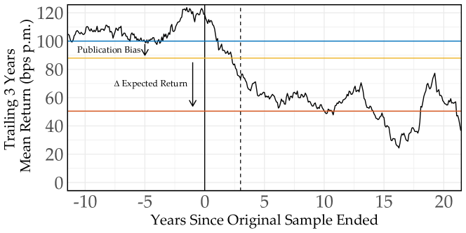
Figure 9: Predictability is 50% Weaker After Publication. Returns are normalized so that the mean in-sample return is 100 bps per month (blue line). Returns are averaged across all CZ22 predictors within each month, then the trailing 36-month mean is computed. The mean post-publication return is in red. Publication bias effects are bounded by decay three years after publication (dashed line). Shrinkage estimates imply half of this decay is publication bias (yellow line). The remaining decay is due to changes in expected returns, which are natural given the claim in many of the original papers that predictability is due to mispricing (e.g. Rosenberg et al. (1985)).

This fact is often mis-interpreted as evidence of pervasive publication bias effects (data snooping, p-hacking, etc). The problem with this interpretation is that monthly predictor returns have very little serial autocorrelation. The mean autocorrelation is 7% at 1 month and falls to zero at 3 months. So return decay driven by publication bias should show up just months after the original samples end, not a decade later. More precisely, publication bias effects are bounded by the 25% decline at year 3 (Fact #2, dashed vertical line).

Multiple testing statistics provide a direct estimate of publication bias effects (Fact # 3, Section 3) and imply a roughly 12% decline (yellow line). The remaining 38% decline, then, is a decline in the expected return. This decline is important for interpreting the economic meaning of predictability, but it is not publication bias.

The economic meaning becomes clear if one reads the original papers. Many, if not most papers argue that their finding is due to mispricing (Rosenberg et al. (1985); Jegadeesh and Titman (1993); etc). Other papers simply present their findings as a puzzle (e.g. Banz (1981); Foster, Olsen, and Shevlin (1984)), which is consistent with the mispricing explanations. In contrast, claiming that mispricing is permanent or that the empirical relationship is somehow structural is less common. It should not be surprising if mispricing is traded away after it is publicized (Marquering et al. (2006)) or if improvements in liquidity decrease mispricing (Chordia et al. (2014)). There’s a reason why this literature is called “anomalies.”

Returns are also about 50% smaller in non-U.S. markets (Jacobs and Müller (2020); Jensen et al. (2022)) and decline similarly in long samples before the original sample periods begin (Linnainmaa and Roberts (2018)). These results further illustrate how anomalies depend on the investing environment. Predictability may rely on the uninformed trades of retail investors (Goetzmann and Huang (2018)) or small, illiquid stocks (Novy-Marx and Velikov (2015)), both of which are less prevalent outside the U.S. (Ke (2018)), and before the original samples begin (typically before 1963). Like post-publication decay, these findings are important for understanding the nature of predictability, but they do not measure publication bias, precisely defined.

4.3 Predictability is about 30% Weaker After Liquidity Adjustments

Finance researchers have long known that predictability is weaker if rebalancing is less frequent (Jegadeesh and Titman (1993)) or if trading is confined to large, liquid stocks (Fama and French (1993); Ball et al. (1995)). This result has a natural interpretation of liquidity effects (Mayshar (1979); Kyle (1985)) and is closely linked to the idea of costly arbitrage (Pontiff (1996); Shleifer and Vishny (1997)). In strategies that avoid illiquidity, arbitrage is more likely, mispricing is smaller, and predictability is weaker.

These early findings turn out to be representative of the broader cross-sectional predictability literature (Novy-Marx and Velikov (2015); Jacobs and Müller (2020); Chen and Velikov (2022)). Figure 10 replicates these results using the CZ22 dataset. The original implementations typically rebalance monthly and almost all equally weight stocks in each leg of the portfolio. Rebalancing annually reduces returns by 25%, as does restricting trading to stocks above the 20th percentile of NYSE market equity. Value-weighting each leg of the portfolio reduces returns even more (roughly 35%).

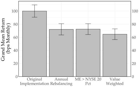
Figure 10: Liquidity Adjustments Decrease Returns by 30%. Data are 207 predictors from CZ22. Grand mean return averages across in-sample months and then averages across predictors. Error bars show to standard errors, approximated by the standard deviation across predictors divided by $\sqrt{207}$. Original implementations follows the original papers. Annual rebalancing updates signal data each year in June. ME $>$ NYSE 20 Pct excludes stocks that fall below the 20th percentile of NYSE market equity. Value-weighted weights stocks by their market equity. Liquidity adjustments robustly decrease expected returns by roughly 30%. Robust effects related to economics should not be equated with data snooping.

Strangely, the recent meta-study literature sometimes cites “data snooping,” or “p-hacking” in connection with Figure 10. Rigorously defined, these terms refer to chance results that are unrelated to economic phenomena (e.g. Lo and MacKinlay (1990); White (2000)). In contrast, the liquidity effects in Figure 10 are robust and founded in classic finance theory.

Liquidity effects are important. One can argue that the original implementations in Figure 10 are irrelevant, and that the liquidity adjustments better capture their potential returns. On the other hand, one can argue that the original implementations provide more powerful tests of classical equilibrium theories, or that investors would combine predictors anyway (DeMiguel et al. (2020)).

These are all arguments about what is the proper “true effect” that one should be trying to measure in Equation (1). These debates require insight into portfolio choice, market equilibrium, and market microstructure, and go far outside the realm of publication bias.

4.4 Loose Language in Meta-Studies

The misinterpretations in Sections 4.1-4.3 are due to loose language. Changes in expected returns should not be equated with data snooping or p-hacking. Many insignificant predictors do not imply multiple testing problems, especially if the significance tests are extremely conservative.

Meta-studies are prone to loose language, as each study covers a lot of ground, making precise language difficult. Meta-studies also use statistics unfamiliar to finance researchers.

However, precise language is possible and important. In everyday life, loose language is spoken and causes confusion. In academic publications, loose language is written down, and can cause confusion for future generations of researchers.

We emphasize the precise usage of language by taking a closer look at two influential meta-studies, Harvey et al. (2016) and Hou et al. (2020).

4.4.1 Harvey, Liu, and Zhu’s (2016) “False Findings”

Harvey, Liu, and Zhu (2016) (HLZ) famously “argue that most findings in financial economics are likely false.” Yet their own estimates imply a false discovery rate of less than 10%. (Section 3.3). So where does HLZ’s famous quote come from?

Their conclusion suggests an answer:

In medical research, the recognition of the multiple testing problem has led to the disturbing conclusion that “most claimed research findings are false” (Ioannidis (2005)). Our analysis of factor discoveries leads to the same conclusion–many of the factors discovered in the field of finance are likely false discoveries: of the 296 published significant factors, 158 would be considered false discoveries under Bonferonni [sic], 142 under Holm, 132 under [Benjamini and Yekutieli (2001) Theorem 1.3] (1%), and 80 under [Benjamini and Yekutieli (2001) Theorem 1.3] (5%).

This passage conflates “most” with “many” and “false discovery” with “insignificant predictor.” 142 out of 296 is not most. And while Bonferroni, Holm (1979), and Benjamini and Yekutieli (2001)’s Theorem 1.3 can determine the number of insignificant results, they cannot determine the number of false discoveries. Using more precise language, HLZ’s claim would be: “many findings in cross-sectional asset pricing are insignificant under some highly conservative multiple testing adjustments” (see Section 4.1)

“False” may seem equivalent to “insignificant,” but these two terms have an important distinction in statistics. In statistics, a “false discovery” or “false rejection” is a significant result that is, in truth, null (Sorić (1989); Benjamini and Hochberg (1995); Storey (2011)). This distinction is fundamental. It is, in essence, “Principal 2” of the American Statistical Association’s “Statement on Statistical Significance and P-Values” (Wasserstein and Lazar (2016)).

This paragraph also cites a theoretical opinion essay (Ioannidis (2005)) as if it is the conclusion of medical research. The empirical counterpart to Ioannidis finds a false discovery rate of only 14% in top medical journals (Jager and Leek (2014)). While this single study has its limitations, review papers find other empirical studies at odds with Ioannidis’s claims, and none in support (Leek and Jager (2017); Fanelli (2018)).

Unfortunately, loose language is echoed in follow-up papers. In fact, HLZ’s citation of Ioannidis (2005) is an example. Ioannidis (2005) claims “[i]t can be proven that most claimed research findings are false.” Yet his claim depends on parameter values that are not universally accepted (e.g., Goodman and Greenland (2007); Christensen and Miguel (2018)). Thus, a more precise claim would be “under certain parameter values, most claimed research findings are false.”

Harvey et al.’s mixing of “insignificant” and “false” is echoed in many papers, including Hou et al. (2020); Chordia et al. (2020); and our own paper Chen and Zimmermann (2022). We urge finance researchers to use precise language and spare future generations of this confusion.

4.4.2 Hou, Xue, and Zhang’s (2020) “Failed Replications” and Microcaps

The second paragraph of Hou et al. (2020) (HXZ) summarizes the paper:

Our key finding is that most anomalies fail to replicate, falling short of currently acceptable standards for empirical finance. First, of the 452 anomalies, 65% cannot clear the single test hurdle of $|t|\geq 1.96$. The key word is “microcaps” Microcaps represent only 3.2% of the aggregate market capitalization but 60.7% of the number of stocks. Microcaps have the highest equal-weighted returns and the largest cross-sectional dispersions in returns and in anomaly variables.

One would assume that HXZ replicate 452 anomalies but that HXZ’s tests fail, mostly because they downweight microcaps. But this is not the case.

Just a few paragraphs later, HXZ explain that microcaps have a minor role:

The failure rate drops to 43.1% if we allow microcaps to run amok with NYSE-Amex-NASDAQ breakpoints and equal-weighted returns.

In other words, microcaps account for only $1-43.1/65=34\%$ of their failed replications.

If it’s not microcaps, then what accounts for the majority of the failed replications? It’s hard to tell because of loose language. HXZ do not define what they consider an “anomaly,” and most of HXZ’s 452 “anomalies” were never shown to obtain $|t|\geq 1.96$ in the original papers (Chen and Zimmermann (2022); Jensen et al. (2022)). So many of the “failed replications” are actually successful replications. For many “anomalies,” HXZ apply “small perturbations to the original variable definitions.” These perturbations are not done systematically, but applied “when necessary.” HXZ do not define when it is necessary, nor do they clearly define which perturbations should be applied when it is necessary. To our reading, the perturbations and their applications can only be described as ad-hoc.

With the missing definition of anomaly and the ad-hoc perturbations, HXZ’s “replication failures” are more precisely described as “insignificant ad-hoc trading strategies.” Given that only about 26% of HXZ’s strategies were shown to clearly produce statistical significance in the original papers (Chen and Zimmermann (2020)), it’s not surprising that roughly half of these ad-hoc strategies are insignificant, even when using equal-weighting.

5 A Framework for Future Research

Outside of cross-sectional predictability, evidence on publication bias in asset pricing is scarce. Perhaps the best evidence on publication bias comes from Goyal and Welch (2008)’s re-examination of 17 equity premium predictors and their on-going update, which adds another 29 predictors (Goyal et al. (2021)).

We conclude by using Goyal and Welch (2008) and Goyal, Welch, and Zafirov (2021) to illustrate how our four facts can be applied to other fields. We focus on real-time forecasts rather than simple regressions (Goyal and Welch (2003); Campbell and Thompson (2008)) for ease of comparison with the real-time results in Sections 2-4. These papers provide the following evidence:

1. How replicable is equity premium predictability? Table 2 of Goyal et al. (2021) suggests that replicability is rather poor. Of 21 predictors that showed point estimates displaying real-time predictability in the original papers, only 10 have the same sign in Goyal et al. (2021)’s replications. Some of these differences are due to differences in the start dates of the real-time tests. These results suggest that either author error or sampling error is has a meaningful impact in Equation (3). Regardless of the exact driver, the reported results are a biased estimate of what a follow-up replication would find.

2. Does equity premium predictability persist out-of-sample? Predictability consistently weakens out-of-sample. But to isolate publication bias effects, one would like to see predictability measures that zoom in on time periods near the original samples, a la McLean and Pontiff (2016). Clear evidence on this question is currently lacking, and might come with large standard errors given the small number of observations relative to the cross-sectional asset pricing literature.

3. Are equity premium prediction p-values much smaller than 0.05? Tables 3-5 of Goyal et al. (2021) strongly suggest the answer is no. Of the 21 predictors that showed real-time predictability in the original papers, none is significant at the 1% level in the replications. Only six out of 21 are significant at the 5% level. While these tests use extended samples including post-sample data, these p-values are so large that it is unlikely that out-of-sample decay matters much. Thus it seems real-time prediction is readily explained by lucky draws, and sampling error in Equation (3) is large.

4. Are equity premium predictors weakly correlated? We downloaded data for Goyal and Welch (2008) from Amit Goyal’s website, signed predictors, and computed correlations. Correlations cluster around zero, and only a small fraction exceed 0.5. While this may sound surprising considering that all variables forecast the same left-hand side variable (the equity premium), it is consistent with the fact that combinations of forecasts predict the equity premium better than any single one of them (Rapach et al. (2010); Rapach and Zhou (2022)), and thus they must provide some uncorrelated variation. Low correlations suggest the p-value statistics in item 3 are good estimates of the underlying probabilities.

Taken together, these results are consistent with publication bias being a major problem in real-time equity premium predictability. But one would like to see more rigorous answers to these questions, such as shrinkage estimates using the exact p-values. One would also like to see the final version of Goyal et al. (2021)’s on-going work, as well as follow-up studies by independent teams. Nevertheless, these four facts show that publication bias certainly varies by the sub-field, and that other fields are not so unaffected by publication bias as cross-sectional predictability. Indeed, the equity premium literature seems to acknowledge these issues, and has more recently focused on methods that combine information from many individual predictors (Rapach and Zhou (2022)).

References

- Akerlof and Michaillat (2018) Akerlof, G. A. and P. Michaillat (2018). Persistence of false paradigms in low-power sciences. Proceedings of the National Academy of Sciences 115(52), 13228–13233.
- Andrews and Kasy (2019) Andrews, I. and M. Kasy (2019). Identification of and correction for publication bias. American Economic Review 109(8), 2766–94.
- Ball et al. (1995) Ball, R., S. Kothari, and J. Shanken (1995). Problems in measuring portfolio performance an application to contrarian investment strategies. Journal of Financial Economics 38(1), 79–107.
- Banz (1981) Banz, R. W. (1981). The relationship between return and market value of common stocks. Journal of financial economics 9(1), 3–18.
- Benjamini (2008) Benjamini, Y. (2008). Comment: Microarrays, empirical bayes and the two-groups model. Statisical Science 23(1), 23–28.
- Benjamini (2020) Benjamini, Y. (2020). Selective inference: The silent killer of replicability.
- Benjamini and Hochberg (1995) Benjamini, Y. and Y. Hochberg (1995). Controlling the false discovery rate: a practical and powerful approach to multiple testing. Journal of the Royal statistical society: series B (Methodological) 57(1), 289–300.
- Benjamini and Yekutieli (2001) Benjamini, Y. and D. Yekutieli (2001). The control of the false discovery rate in multiple testing under dependency. Annals of statistics, 1165–1188.
- Benjamini and Yekutieli (2005) Benjamini, Y. and D. Yekutieli (2005). False discovery rate–adjusted multiple confidence intervals for selected parameters. Journal of the American Statistical Association 100(469), 71–81.
- Bessembinder et al. (2021) Bessembinder, H., A. Burt, and C. M. Hrdlicka (2021). Time series variation in the factor zoo. Aaron Paul and Hrdlicka, Christopher M., Time Series Variation in the Factor Zoo (December 22, 2021).
- Brodeur et al. (2016) Brodeur, A., M. Lé, M. Sangnier, and Y. Zylberberg (2016). Star wars: The empirics strike back. American Economic Journal: Applied Economics 8(1), 1–32.
- Campbell et al. (2008) Campbell, J. Y., J. Hilscher, and J. Szilagyi (2008). In search of distress risk. The Journal of Finance 63(6), 2899–2939.
- Campbell and Thompson (2008) Campbell, J. Y. and S. B. Thompson (2008). Predicting excess stock returns out of sample: Can anything beat the historical average? The Review of Financial Studies 21(4), 1509–1531.
- Card and DellaVigna (2020) Card, D. and S. DellaVigna (2020). What do editors maximize? evidence from four economics journals. Review of Economics and Statistics 102(1), 195–217.
- Chen (2021) Chen, A. Y. (2021). The limits of p-hacking: Some thought experiments. The Journal of Finance 76(5), 2447–2480.
- Chen (2022) Chen, A. Y. (2022). Do t-statistic hurdles need to be raised? arXiv preprint arXiv:2204.10275.
- Chen and Velikov (2022) Chen, A. Y. and M. Velikov (2022). Zeroing in on the expected returns of anomalies. Journal of Financial and Quantitative Analysis.
- Chen and Zimmermann (2018) Chen, A. Y. and T. Zimmermann (2018). Publication bias and the cross-section of stock returns. https://www.federalreserve.gov/econres/feds/files/2018033pap.pdf.
- Chen and Zimmermann (2020) Chen, A. Y. and T. Zimmermann (2020). Publication bias and the cross-section of stock returns. The Review of Asset Pricing Studies 10(2), 249–289.
- Chen and Zimmermann (2022) Chen, A. Y. and T. Zimmermann (2022). Open source cross sectional asset pricing. Critical Finance Review.
- Chinco et al. (2021) Chinco, A., A. Neuhierl, and M. Weber (2021). Estimating the anomaly base rate. Journal of financial economics 140(1), 101–126.
- Chordia et al. (2020) Chordia, T., A. Goyal, and A. Saretto (2020). Anomalies and false rejections. The Review of Financial Studies 33(5), 2134–2179.
- Chordia et al. (2014) Chordia, T., A. Subrahmanyam, and Q. Tong (2014). Have capital market anomalies attenuated in the recent era of high liquidity and trading activity? Journal of Accounting and Economics 58(1), 41–58.
- Christensen and Miguel (2018) Christensen, G. and E. Miguel (2018). Transparency, reproducibility, and the credibility of economics research. Journal of Economic Literature 56(3), 920–80.
- De Long and Lang (1992) De Long, J. B. and K. Lang (1992). Are all economic hypotheses false? Journal of Political Economy 100(6), 1257–1272.
- DeMiguel et al. (2020) DeMiguel, V., A. Martín-Utrera, F. J. Nogales, and R. Uppal (2020). A Transaction-Cost Perspective on the Multitude of Firm Characteristics. The Review of Financial Studies 33(5), 2180–2222.
- Efron (2011) Efron, B. (2011). Tweedie’s formula and selection bias. Journal of the American Statistical Association 106(496), 1602–1614.
- Efron (2012) Efron, B. (2012). Large-scale inference: empirical Bayes methods for estimation, testing, and prediction, Volume 1. Cambridge University Press.
- Fama and French (1993) Fama, E. F. and K. R. French (1993). Common risk factors in the returns on stocks and bonds. Journal of financial economics 33(1), 3–56.
- Fanelli (2018) Fanelli, D. (2018). Is science really facing a reproducibility crisis, and do we need it to? Proceedings of the National Academy of Sciences 115(11), 2628–2631.
- Farcomeni (2007) Farcomeni, A. (2007). Some results on the control of the false discovery rate under dependence. Scandinavian Journal of Statistics 34(2), 275–297.
- Ferreira and Zwinderman (2006) Ferreira, J. and A. Zwinderman (2006). On the benjamini–hochberg method. The Annals of Statistics 34(4), 1827–1849.
- Fisher (1925) Fisher, R. (1925). Statistical methods for research workers.
- Foster et al. (1984) Foster, G., C. Olsen, and T. Shevlin (1984). Earnings releases, anomalies, and the behavior of security returns. Accounting Review, 574–603.
- Francis et al. (2004) Francis, J., R. LaFond, P. M. Olsson, and K. Schipper (2004). Costs of equity and earnings attributes. The accounting review 79(4), 967–1010.
- Genovese et al. (2006) Genovese, C. R., K. Roeder, and L. Wasserman (2006). False discovery control with p-value weighting. Biometrika 93(3), 509–524.
- Goetzmann and Huang (2018) Goetzmann, W. N. and S. Huang (2018). Momentum in imperial russia. Journal of Financial Economics 130(3), 579–591.
- Goodman and Greenland (2007) Goodman, S. and S. Greenland (2007). Why most published research findings are false: problems in the analysis. PLoS medicine 4(4), e168.
- Goyal and Welch (2003) Goyal, A. and I. Welch (2003). Predicting the equity premium with dividend ratios. Management Science 49(5), 639–654.
- Goyal and Welch (2008) Goyal, A. and I. Welch (2008). A comprehensive look at the empirical performance of equity premium prediction. The Review of Financial Studies 21(4), 1455–1508.
- Goyal et al. (2021) Goyal, A., I. Welch, and A. Zafirov (2021). A comprehensive look at the empirical performance ofequity premium prediction ii. Available at SSRN 3929119.
- Green et al. (2013) Green, J., J. R. Hand, and X. F. Zhang (2013). The supraview of return predictive signals. Review of Accounting Studies 18(3), 692–730.
- Green et al. (2017) Green, J., J. R. Hand, and X. F. Zhang (2017). The characteristics that provide independent information about average us monthly stock returns. The Review of Financial Studies 30(12), 4389–4436.
- Hamermesh (2007) Hamermesh, D. S. (2007). Replication in economics. Canadian Journal of Economics/Revue canadienne d’économique 40(3), 715–733.
- Harvey et al. (2016) Harvey, C. R., Y. Liu, and H. Zhu (2016). … and the cross-section of expected returns. The Review of Financial Studies 29(1), 5–68.
- Holm (1979) Holm, S. (1979). A simple sequentially rejective multiple test procedure. Scandinavian journal of statistics, 65–70.
- Hou et al. (2020) Hou, K., C. Xue, and L. Zhang (2020). Replicating anomalies. The Review of Financial Studies 33(5), 2019–2133.
- Ioannidis (2005) Ioannidis, J. P. (2005). Why most published research findings are false. PLoS medicine 2(8), e124.
- Jacobs and Müller (2018) Jacobs, H. and S. Müller (2018). … and nothing else matters? on the dimensionality and predictability of international stock returns. On the Dimensionality and Predictability of International Stock Returns (November 20, 2018).
- Jacobs and Müller (2020) Jacobs, H. and S. Müller (2020). Anomalies across the globe: Once public, no longer existent? Journal of Financial Economics 135(1), 213–230.
- Jager and Leek (2014) Jager, L. R. and J. T. Leek (2014). An estimate of the science-wise false discovery rate and application to the top medical literature. Biostatistics 15(1), 1–12.
- Jegadeesh and Titman (1993) Jegadeesh, N. and S. Titman (1993). Returns to buying winners and selling losers: Implications for stock market efficiency. The Journal of finance 48(1), 65–91.
- Jensen et al. (2022) Jensen, T. I., B. T. Kelly, and L. H. Pedersen (2022). Is there a replication crisis in finance?
- Ke (2018) Ke, D. (2018). Cross-country differences in household stock market participation: The role of gender norms. In AEA Papers and Proceedings, Volume 108, pp. 159–162. JSTOR.
- Kuhn (1962) Kuhn, T. S. (1962). The structure of scientific revolutions, Volume 111. Chicago University of Chicago Press.
- Kyle (1985) Kyle, A. S. (1985). Continuous auctions and insider trading. Econometrica: Journal of the Econometric Society, 1315–1335.
- Leek and Jager (2017) Leek, J. T. and L. R. Jager (2017). Is most published research really false? Annual Review of Statistics and Its Application 4, 109–122.
- Linnainmaa and Roberts (2018) Linnainmaa, J. T. and M. R. Roberts (2018). The history of the cross-section of stock returns. The Review of Financial Studies 31(7), 2606–2649.
- Lo and MacKinlay (1990) Lo, A. W. and A. C. MacKinlay (1990). Data-snooping biases in tests of financial asset pricing models. The Review of Financial Studies 3(3), 431–467.
- Marquering et al. (2006) Marquering, W., J. Nisser, and T. Valla (2006). Disappearing anomalies: a dynamic analysis of the persistence of anomalies. Applied financial economics 16(4), 291–302.
- Mayshar (1979) Mayshar, J. (1979). Transaction costs in a model of capital market equilibrium. Journal of Political Economy 87(4), 673–700.