Forecasting Vehicle Pitch of a Lightweight Underwater Vehicle Manipulator System with Recurrent Neural Networks

Abstract

As Underwater Vehicle Manipulator Systems (UVMSs) have gotten smaller and lighter over the past years, it is becoming increasingly important to consider the coupling forces between the manipulator and the vehicle when planning and controlling the system. However, typical methods of handling these forces require an exact hydrodynamic model of the vehicle and access to low-level torque control on the manipulator, both of which are uncommon in the field. Therefore, many UVMS control methods are kinematics-based, which cannot inherently account for these effects. Our work bridges the gap between kinematic control and dynamics by training a recurrent neural network on simulated UVMS data to predict the pitch of the vehicle in the future based on the system’s previous states. Kinematic planners and controllers can use this metric to incorporate dynamic knowledge without a computationally expensive model, improving their ability to perform underwater manipulation tasks.

I Introduction

According to a recent study, man-made structures covered 32,000 km² of the ocean floor in 2018, projected to increase to 39,400 km² by 2028 [1]. These structures need to be inspected and maintained to ensure that leaks and environmental impacts are monitored and kept to a minimum. Underwater Vehicle Manipulator Systems (UVMSs) are more suited for this task than human divers because deploying them poses less risk to humans and does not require long depressurization times. Additionally, whereas large work-class UVMSs are expensive to deploy, smaller inspection class vehicles are becoming cheaper, lighter, and more accessible, making them ideal to deploy on a wider scale for these tasks.

However, lightweight UVMSs face challenges that larger vehicles do not. In particular, manipulator motion causes the vehicle to move, an important factor to consider in the motion planning phase. When using an inverse dynamics scheme (e.g. computed torque) for control, this problem becomes trivial. Unfortunately, many commercial underwater manipulators don’t permit low-level torque control, and this method also requires a difficult-to-obtain accurate dynamic model of the UVMS – complete with hydrodynamic terms and thruster models – so inverse kinematics is commonly used instead. However, kinematic models do not have knowledge of the dynamic effects of the manipulator, so other methods of incorporating dynamic knowledge must be employed.

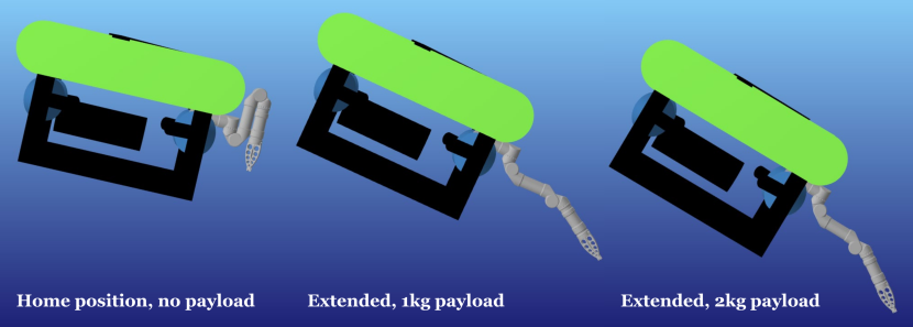
Figure 1: A lightweight UVMS. (Left) The vehicle pitches slightly forward with the manipulator carrying no payload and stored in the home configuration. The vehicle pitches further when the arm is extended while supporting 1 kg (center) and the maximum 2 kg payloads (right).

Current solutions tend to rely on proxy measures, such as by constraining manipulator movement to a box [2], but minimizing manipulator motion in this way unnecessarily constrains the operational workspace and does not provide any information about the quality or risk of the manipulator’s configuration. Additionally, smaller vehicles are often underactuated, and thus cannot provide counter forces in all directions. In these cases, knowing the extent to which the manipulator motion would unbalance the vehicle is particularly important, especially during tasks requiring precision manipulation (Figure 1).

In this paper we present a model that predicts the effects of manipulator motion on vehicle pitch. We developed a UVMS simulator in Julia combining rigid body dynamics and hydrodynamics, and simulated thousands of manipulator trajectories with it (Section III). Using this data, we trained two types of Recurrent Neural Networks (RNNs): one that predicts only pitch, and one that uses an autoregressive approach (Section IV). We show that our network can effectively learn both the nonlinear dynamics of the system and the controller to predict vehicle pitch 4 seconds in advance, and is robust to common inaccuracies in the hydrodynamic coefficients (Section V). Incorporating this model, kinematic whole body controllers and planners could predict how a vehicle will move in response to manipulator motions, thus providing the potential for improved end-effector accuracy/precision during underwater manipulation (Section VI).

II Related Work

II-A Coupling Effects

When a manipulator is attached to an underwater vehicle, forces are transmitted between the two systems, an effect called coupling. Schempf and Yoerger [3] were one of the first to recognize the adverse effects of ignoring coupling forces in 1992. The authors demonstrated that even a 20:1 mass ratio between the vehicle and the manipulator caused significant unwanted coupling effects. Other researchers later confirmed that modeling the hydrodynamic effects was essential to station keeping and end effector accuracy [4, 5].

The coupling effect has become a more prescient problem in recent years as underwater vehicles have become more lightweight. In particular, Barbalata et. al extensively explored the coupling effect on a lightweight UVMS in simulation in [6, 7]. Because the authors used a computed torque control scheme, they were able to calculate the coupling forces and compensate for them with the controller. Similarly, the Ocean One UVMS uses a whole-body computed torque controller to account for coupling effects on their custom-built system [8].

Most off-the-shelf, commercial underwater manipulators do not provide low-level torque control, which precludes the use of computed torque controllers. Therefore, in practice, most whole body controllers for UVMSs are kinematics based, such as SAUVIM [9], TRIDENT [10], MARIS [11], and ROBUST [12]. Recently, the DexROV project showed promising whole-body kinematic control results in a kinematics-only simulation. However, during sea trials the vehicle was clamped to an underwater structure, negating the need to understand the coupling effect [13]. Kinematically, the manipulator was constrained to a virtual box to prevent self-collisions and over-extension [2].

Traditionally, UVMSs have a large vehicle-to-manipulator mass ratio, and can thus safely ignore coupling. However, as vehicles get smaller and more lightweight, control schemes need to be developed that handle the dynamic coupling effect while using a kinematic control scheme, something that has not yet been effectively demonstrated in the literature.

II-B Recurrent Neural Networks for Motion Prediction

Recurrent neural networks are used when time is a significant dimension of the data, or when the input to the network is a variable-length sequence. Sequence-to-sequence networks are commonly used for machine translation [14] and human motion prediction [15]. They are particularly suited for motion predictions, as time-dependent elements can be captured and modeled.

Recurrent neural networks have been applied to ships and Unmanned Surface Vehicles (USVs), which are comparable to UVMSs in size, but sit above water and do not have manipulation capabilities. D’agostino et al. use RNNs on ships in a high sea state to predict the ship’s motion 20 seconds ahead based on sensor and control data [16]. Zhang et al. use a combination of Convolutional Neural Networks and RNNs to predict the roll of a USV from real-time sensor data [17]. Similarly, Yang et al. use neural networks to predict a ship’s attitude under disturbances from waves [18]. However, RNNs have not been applied to dynamically coupled systems such as UVMSs.

Human motion prediction is one of the most common applications in this field. Fragkiadaki introduced Encoder-Recurrent-Decoder networks in [15]. A particularly useful architecture was proposed by Martinez et al. in [19]. They proposed feeding the network its own predictions in place of adding noise, so the network learns to correct its own mistakes. They also suggest a residual connection, such that the network learns the differential between two states instead of the next state itself. Our network architecture is heavily modeled after Martinez’s.

III Methodology

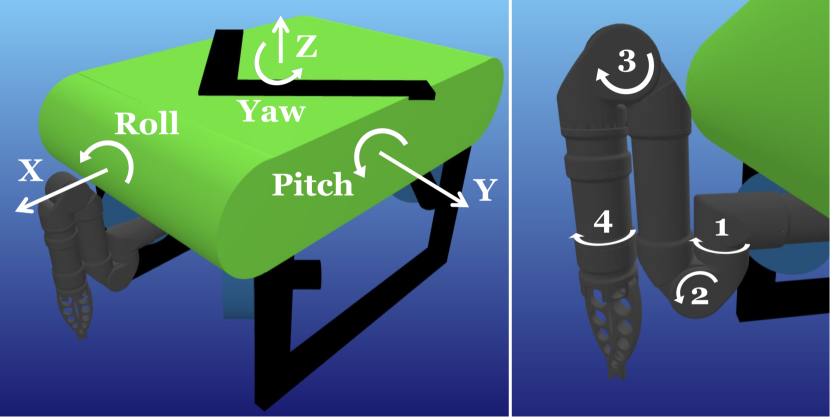
Figure 2: Images of the Seatbotix/Alpha UVMS, as visualized in MeshCat from the Julia simulation. (Left) A right-handed Cartesian coordinate frame is assigned at the vehicle’s center of mass, using forward-left-up notation. (Right) The Alpha’s four joints: a base joint in yaw, two joints to extend the arm, and a rotational joint at the wrist.

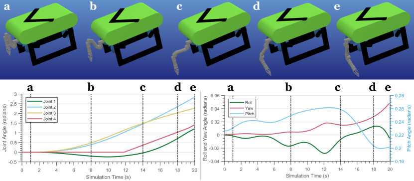
Figure 3: (Top) Snapshots of the MeshCat visualization of the UVMS performing an example trajectory. (Bottom left) Manipulator joint angles over time. (Bottom right) Roll, pitch, and yaw of the vehicle over time.

To train a deep learning model, we first needed a large data set of realistic UVMS motions. Section III-A describes the simulator we developed. The algorithms for trajectory generation and control are described in Section III-B. Finally, we discuss the specifics of the neural network architecture used to predict pitch in Section III-C.

III-A Simulation Environment

The system comprises a Teledyne Seabotix (San Diego, CA, USA) vLBV300 vehicle [20] and a Reach Robotics (Sydney, Australia) Alpha 5 electric manipulator [21]. The Seabotix vehicle has 4 actuated degrees of freedom (surge, sway, heave, and yaw) and two unactuated degrees which are passively stable (pitch and roll). The Alpha has 4 rotational degrees of freedom and a gripper end effector. Figure 2 is a visual representation of the system and its degrees of freedom. Values for mass, body geometry, buoyancy, and manipulator drag coefficients were obtained from the manufacturer’s documentation. Drag coefficients for the vehicle were taken from previous approximations with Computational Fluid Dynamics in [22]. The added mass was approximated by scaling down the added mass of the ROV Minerva [23] to match the added mass calculated in [22] for the Seabotix vehicle. Similarly, we used the same nonlinear/linear drag coefficient ratio as [23] to estimate the linear drag coefficients for the vehicle. The added mass for the manipulator approximated each link as a cylinder.

The simulator was written in the Julia programming language [24] using primarily the RigidBodyDynamics.jl package [25]. Fossen’s equation is applied to the vehicle [26]:

$$M\mathcal{\dot{V}}+C(\mathcal{V})\mathcal{V}+D(\mathcal{V})\mathcal{V}+g(\eta)=\tau$$ (1)

where $\mathcal{V}$ is the spatial velocity vector of the vehicle in the body-fixed frame, $M$ is the inertia matrix, $C(\mathcal{V})$ is the matrix of Coriolis and centripetal terms, $D(\mathcal{V})$ is the damping matrix, $g(\eta)$ is the vector of gravitational forces and moments (where $\eta$ refers to the vehicle’s pose in the world frame) as well as buoyancy effects, and $\tau$ is the vector of control inputs and external forces. $M$ and $C(\mathcal{V})$ both include a rigid body term and an added mass term: $M=M_{RB}+M_{A}$ and $C(\mathcal{V})=C_{RB}(\mathcal{V})+C_{A}(\mathcal{V})$. Drag on the vehicle is approximated as the summation of a linear term and a quadratic term.

All of the hydrodynamic forces applied to the vehicle are applied to the manipulator as well, except linear drag is not included. Hydrodynamic forces are applied as external wrenches to the manipulator; i.e. Fossen’s equations are not solved for each link individually.

III-B Trajectory Generation

In this work, we are interested in how motions of the manipulator affect motions of the vehicle. Therefore, we employed a PID controller in the simulation environment to keep the vehicle’s center of mass stationary in surge, sway, and heave. Each trajectory starts with the UVMS at the equilibrium position (top left snapshot in Figure 3) and ends at a random reachable position and velocity for each joint, using a quintic trajectory in joint space to interpolate between them, ignoring self collisions. An example trajectory is shown in Figure 3. Additionally, a random time scaling between 1x and 3x was applied to the trajectory, such that it does not always attempt to complete the trajectory in the shortest amount of time.

Each joint is individually controlled with a velocity PID controller, one of the options for control on the hardware. In simulation, each joint obeys torque limits and can only change its torque a limited amount per time step. The controller is assumed to have perfect knowledge of the system state.

Simulations were completed with a time step and control loop of 1kHz, which was down-sampled to 50Hz before being used in the network. The simulation gathers 24 data streams, separated into several categories, as shown in Table I, rows 1-7. Vehicle positions are w.r.t. the world frame; vehicle velocities are expressed in the vehicle (body) frame. All angles are in rad and angular velocities are in rad/s.

In addition, for each trajectory, the start and goal waypoints are saved, as shown in Table I, rows 8-9. Minor post-processing was done: a 15-point moving average was applied to all velocities; and since RigidBodyDynamics.jl outputs vehicle orientations as quaternions, they were translated to roll-pitch-yaw coordinates. Each data stream was separately normalized to have a mean of 0 and standard deviation of 1.

TABLE I: Simulator Output Data Streams

Gp. #	Data Stream Description	# Chan.
1	Vehicle X, Y, Z positions	3
2	Vehicle X, Y, Z velocities	3
3	Vehicle roll, pitch, and yaw	3
4	Vehicle angular velocities	3
5	Manipulator joint positions	4
6	Manipulator joint velocities	4
7	Manipulator desired joint velocities	4
8	Manip. joint position waypoints	8
9	Manip. joint velocity waypoints	8

III-C Network

The two most common recurrent units are Long Short-Term Memory units (LSTMs) and Gated Recurrent Networks (GRUs). These have been compared many times and have typically been found to be comparable in performance [27]. We use GRUs in our network to model work done by [19].

We primarily studied two architectures for pitch prediction: an autoregressive method and a pitch-only prediction. Networks were trained with MATLAB’s Deep Learning Toolbox [28]. The pitch-only prediction takes all of the data streams as inputs, and outputs k steps of predictions for the future pitch of the vehicle, shown graphically in Figure 4. It has a single GRU layer and a fully connected layer to reduce it to k outputs. Its architecture is shown in Figure 6b.

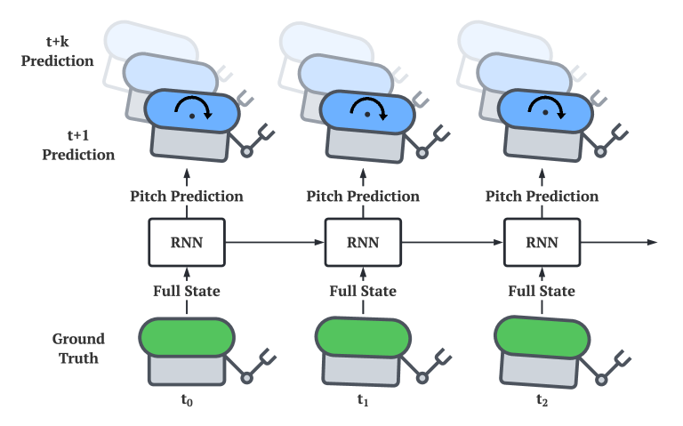
Figure 4: Pitch-only predictions. At each time step, the ground truth state is fed into the system, and k steps of vehicle pitch are predicted.

The autoregressive method is modeled off work completed in [19], and shown graphically in Figure 6a. It takes the continuous data streams (Groups 1-7 from Table I) as input to a GRU layer. Those outputs are concatenated with the waypoint data (Groups 8-9) and sent through the fully connected layer. This output is added to the state data inputs with a residual connection, such that the network is learning the change in state, not the new state itself. The output of this network is the entire state of the UVMS at the next time step. This prediction can be fed back into the network as inputs recursively to forecast k steps ahead (Figure 5).

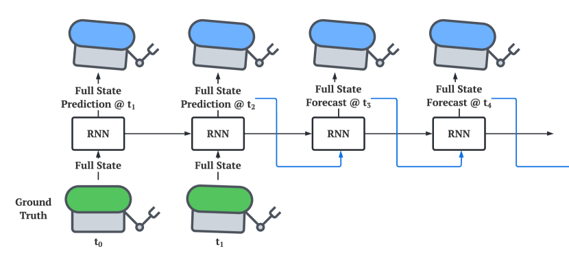
Figure 5: The autoregressive network. Blue lines represent predictions fed back into the network. Here, ground truth is fed into the network until $t_{1}$, at which point it uses its full-state prediction for $t_{2}$ to forecast the state at $t_{3}$, and so on until forecasting $k$ steps ahead.

For each mini-batch, the autoregressive network chooses 16 random trajectories. It predicts only the next step (blue dashed lines in Figure 6a) until a random time step, when it starts forecasting instead (yellow lines in Figure 6a). The network forecasts k steps ahead and uses those 16 forecasts to train. The loss is calculated along the entire trajectory, not just the forecast, to keep single-step predictions accurate.

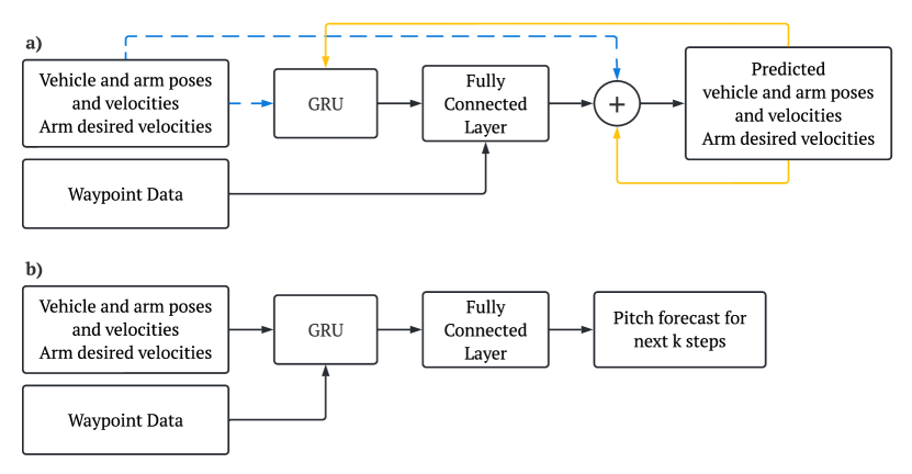
Figure 6: Comparison of network architectures. (a) The autoregressive network. Blue dashed lines denote data flow for a one-step prediction; yellow lines denote flow for a forecast. (b) The pitch-only prediction network.

IV Experiments

Unless stated otherwise, the pitch-only prediction network is trained with 5000 trajectories from the simulator. 95% of the data was used for training and 5% for validation. The network has 384 GRU units and is trained for 100 epochs. The network is optimized with Adam [29], and started with a learning rate of 0.001, reduced by a factor of 0.9 every 5 epochs. The network is validated 5 times per epoch, and the output network is the step with the lowest validation loss. The network predicts 25 steps ahead ($k=25$) for a prediction time of 0.5s given the input frequency of 50Hz.

IV-A Feature Ablation

First, we ran an ablation study to determine the order of importance of the input features. We grouped the data inputs into 9 feature groups as described in Table I, but kept the pitch and corresponding angular velocity value for all of the trials. We used standard backwards-elimination: at each step, we trained n networks, each with n-1 feature groups included, and eliminated the feature group with the lowest validation loss. The study was repeated, now with n-1 networks, each with n-2 feature groups included, and so on.

For this ablation study, we used the pitch-only prediction network (Figure 4) as it had a much shorter training time. To further decrease training time, we simplified the network to 128 GRU units and trained the network for 50 epochs. The learning rate dropped by a factor of 0.8 every epoch. Each network was trained 3 separate times, and the average validation loss was taken between the three trials to determine the feature group with the least impact.

IV-B Pitch Prediction over Longer Periods

Next, we explored how the two network architectures compare on how far in the future they can predict the vehicle pitch. Using the same pitch-only architecture with 25 outputs, we retrained the network to predict every other step, every third step, and so on, resulting in predictions 0.5 to 4s long in increments of 0.5s. Three networks were trained for each prediction length.

The autoregressive network was first trained on ground truth single-step predictions for 50 epochs with 384 GRU units, with an identical learning rate drop to the pitch prediction network. After that, forecasts were used as data inputs as described in Section III-C for another 50 epochs. To balance training time and accuracy, the input frequency was decreased to 10Hz for this network such that each second of prediction requires 10 forecasts. The network was only trained on 0.5s, 1s, 2s, 3s, and 4s forecasts, as these took significantly longer than the pitch-only network to train.

IV-C Pitch Prediction under Uncertain Hydrodynamics

Whereas many of the dynamic parameters of the system can be found analytically, such as the mass distribution, geometry, and buoyancy, some values are incredibly difficult to find, such as the added mass and drag terms. In the literature, these terms tend to be estimated or scaled from other, similar UVMSs. As such, it is likely that the estimations we used to build a simulator are not the actual parameters of the physical system. Therefore, our next experiment explores how uncertain hydrodynamic parameters affect the accuracy of the pitch predictions.

First, we created a testing database of slightly incorrect models by adding noise to several terms individually: the vehicle linear drag and quadratic drag coefficients; the manipulator drag coefficients; the vehicle added mass; and the manipulator added mass. For each parameter, we generated ten models each that were incorrect by up to 1%, 10%, and 50%. We simulated 50 random trajectories for each of these instances. We tested these datasets on the standard pitch-only prediction network described in Section IV.

V Results & Discussion

V-A Feature Ablation

The order of importance of the feature groups as determined from the ablation study are listed in Table II. The network performance after each feature set was eliminated, quantified as the root mean squared error (RMSE) over the validation dataset, is shown in Figure 7.

TABLE II: Ablation Study Results

	Group Name
1	Vehicle orientation	(Group 3)
2	Manipulator joint positions	(Group 5)
3	Vehicle angular velocities	(Group 4)
4	Vehicle linear velocities	(Group 2)
5	Manipulator desired velocities	(Group 7)
6	Vehicle linear positions	(Group 1)
7	Joint velocity waypoints	(Group 9)
8	Manipulator velocities	(Group 6)
9	Joint position waypoints	(Group 8)

At the highest importance, we have vehicle orientation and manipulator joint positions. The higher importance of manipulator position over velocity implies that we have a system operating at a slow enough time scale that it is almost at equilibrium at each time step.

Near the bottom of the list, we found that waypoint data and manipulator velocities were least important to the prediction. We believe the desired manipulator velocities and actual velocities were redundant, making only one necessary for predictions. There are a number of reasons the waypoint data could be ranked low: we are predicting a short enough time span that the goal states are not useful; the waypoint data is constant, so recurrent networks are unsuited to handling them; or, they simply had too many channels, and eliminating them allowed the network to train other units better in the allotted time. We expect that for a longer prediction, goal states might have more utility.

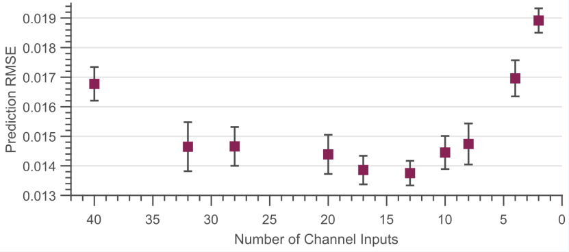
Figure 7: The validation RMSE on a 25-step prediction after 50 epochs as data streams are eliminated in the order listed in Table II. The error is minimized between 13 and 17 feature inputs.

From Figure 7, we see the best validation loss was achieved with 13-17 input channels, including the vehicle orientation and velocities, and the manipulator joint positions and desired velocities. Whereas an decrease in error in previous eliminations could be attributed to having fewer inputs and therefore fewer weights to train, the increase in error when using fewer than 13 inputs clearly represents a loss of important information, and thus all of those inputs should be kept in future iterations of the network. For the remaining experiments, only the top 5 feature groups were kept as inputs to the network, which brought the number of inputs down to 17 from the 40 original streams.

V-B Pitch Prediction over Longer Periods

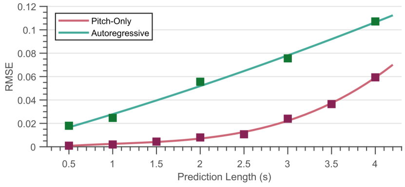
Figure 8: RMSE on the forward forecast as the prediction length increases on the pitch-only network (red) and the autoregressive network (green).

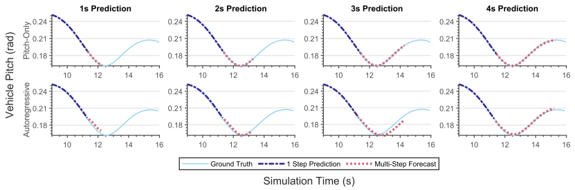
Figure 9: Ground truth and predicted pitch over increasing periods of time on a trajectory in the validation set. The dark blue dashed line represents just the first pitch prediction at a step; the pink dashed line shows all steps of the forward forecast.

Figure 8 compares the performance of the pitch-only network and the autoregressive network on increasing forecast lengths, quantified as the RMSE over the forward prediction. For a fair comparison, ground truth data was fed in for at least 25 steps before forecasting forward regardless of data stream frequency. The pitch-only prediction network error increases exponentially over prediction length, whereas the autoregressive network error increases linearly; however, on the prediction lengths tested, the pitch-only network was consistently superior to the autoregressive one.

The predictions remain useful for a significant period of time. Figure 9 shows plots of the actual pitch angle and prediction on a validation trajectory. The predictions remain qualitatively reasonable: they predict a realistic direction and smooth movement. The pitch-only network matches the ground truth trajectory more precisely overall.

Using MATLAB’s trainNetwork function on an NVIDIA GeForce RTX 3060 GPU (Santa Clara, CA), forward predictions require 48ms of overhead and 0.1ms for each time step when all data is fed in at once. Predictions that take new data on each time step take 4ms per step. Therefore, the pitch-only prediction takes 4ms to predict 25 steps ahead regardless of prediction length, whilst the autoregressive network takes 4ms per step, e.g. on a 10Hz data stream, it takes 20ms for a 0.5s prediction, 40ms for a 1s prediction, and so on.

Between the prediction time, the RMSE, and the qualitative results, the pitch-only network outperforms the autoregressive network. It runs quicker than a standard control loop, making it feasible to use for real-time control. The autoregressive method takes longer and is less accurate, but provides more information about the state of the vehicle besides the pitch, potentially useful for offline applications.

V-C Pitch Prediction under Uncertain Hydrodynamics

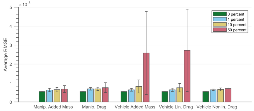
Figure 10: RMSEs on test datasets with variations in hydrodynamic terms.

Figure 10 shows the robustness of the network to incorrect hydrodynamic parameters. In general, the network is resilient to differences in the hydrodynamic parameters, with the exception that a high error in the vehicle added mass or linear drag had an outsized effect on the prediction capabilities. These are likely the most influential because they are the most directly related to vehicle pitch: the more added mass the vehicle has, the higher its effective inertia, and the less the vehicle will move in response to forces. Similarly, the drag on the vehicle dictates how quickly the system dampens the pitch oscillation caused by the manipulator.

One main flaw of our work is that the model is not generalizable. If the configuration of the UVMS changes in any way, the model will have to be retrained. Luckily, our network is robust to minor changes in hydrodynamics, so changes to the distribution of the mass of the vehicle would be the driving factor of retraining.

VI Conclusion

Overall, our RNN was able to very closely predict the pitch of the vehicle even several seconds ahead on a small network with short computation time. Working in our favor were several factors. We only used one kind of simple trajectory in training and testing, for which the path between any two given points is deterministic. Therefore, even though the network has to learn the controller and the dynamics, it has all the information it needs to calculate its path exactly. A controller that relies on external information may need a different network, in which that information is also included as inputs.

Since we have tested exclusively in simulation, we assume perfect knowledge of the system state. This would not be realistic in underwater hardware, where sensor noise and localization errors are common. One next step would be to explore how realistic, artificially added sensor noise would affect the results, and whether the adverse affects could be remedied with data augmentation.

Regardless, our work provides a fast-to-compute model for predicting the future pitch of the vehicle based on its previous state. It can be used in Model Predictive Control schemes, in planning algorithms, or in kinematic whole-body control schemes to improve the end-effector accuracy of lightweight UVMSs.

References

- [1] A. B. Bugnot, M. Mayer-Pinto, L. Airoldi, E. C. Heery, E. L. Johnston, L. P. Critchley, E. M. Strain, R. L. Morris, L. H. Loke, M. J. Bishop, E. V. Sheehan, R. A. Coleman, and K. A. Dafforn, “Current and projected global extent of marine built structures,” Nature Sustainability 2020 4:1, vol. 4, pp. 33–41, 8 2020.
- [2] P. D. Lillo, D. D. Vito, and G. Antonelli, “Set-based inverse kinematics control of an uvms within the dexrov project,” OCEANS 2018 MTS/IEEE Charleston, 1 2019.
- [3] H. Schempf and D. R. Yoerger, “Coordinated vehicle/manipulation design and control issues for underwater telemanipulation,” IFAC Proceedings Volumes, vol. 25, pp. 259–267, 4 1992.
- [4] H. H. Wang, S. M. Rock, and M. J. Lee, “Experiments in automatic retrieval of underwater objects with an auv,” Oceans Conference Record (IEEE), vol. 2, pp. 366–373, 1995.
- [5] V. Rigaud, E. Coste-Maniere, M. J. Aldon, P. Probert, M. Perrier, P. Rives, D. Simon, D. Lane, J. Kiener, A. Casals, J. Amat, P. Dauchez, and M. Chantler, “Union: Underwater intelligent operation and navigation,” IEEE Robotics and Automation Magazine, vol. 5, pp. 25–34, 3 1998.
- [6] C. Barbălată, M. W. Dunnigan, and Y. Pétillot, “Dynamic coupling and control issues for a lightweight underwater vehicle manipulator system,” in 2014 Oceans-St. John’s. IEEE, 2014, pp. 1–6.
- [7] C. Barbălată, M. W. Dunnigan, and Y. Petillot, “Coupled and decoupled force/motion controllers for an underwater vehicle-manipulator system,” Journal of Marine Science and Engineering, vol. 6, pp. 1–23, 2018.
- [8] G. Brantner and O. Khatib, “Controlling ocean one: Human–robot collaboration for deep-sea manipulation,” Journal of Field Robotics, 2020.
- [9] G. Marani, S. K. Choi, and J. Yuh, “Underwater autonomous manipulation for intervention missions auvs,” Ocean Engineering, vol. 36, pp. 15–23, 1 2009.
- [10] P. J. Sanz, P. Ridao, G. Oliver, G. Casalino, Y. Petillot, C. Silvestre, C. Melchiorri, and A. Turetta, “Trident an european project targeted to increase the autonomy levels for underwater intervention missions,” in 2013 OCEANS - San Diego, 2013, pp. 1–10.
- [11] E. Simetti and G. Casalino, “Whole body control of a dual arm underwater vehicle manipulator system,” Annual Reviews in Control, vol. 40, pp. 191–200, 1 2015.
- [12] “Sliding mode impedance control for contact intervention of an i-auv: Simulation and experimental validation,” Ocean Engineering, vol. 196, p. 106855, 1 2020.
- [13] P. D. Lillo, E. Simetti, F. Wanderlingh, G. Casalino, and G. Antonelli, “Underwater intervention with remote supervision via satellite communication: Developed control architecture and experimental results within the dexrov project,” IEEE Transactions on Control Systems Technology, vol. 29, pp. 108–123, 1 2021.
- [14] I. Sutskever, O. Vinyals, and Q. V. Le, “Sequence to sequence learning with neural networks,” 2014.
- [15] K. Fragkiadaki, S. Levine, P. Felsen, and J. Malik, “Recurrent network models for human dynamics,” 2015.
- [16] D. D’Agostino, A. Serani, F. Stern, and M. Diez, “Recurrent-type neural networks for real-time short-term prediction of ship motions in high sea state,” arXiv preprint arXiv:2105.13102, 2021.
- [17] W. Zhang, P. Wu, Y. Peng, and D. Liu, “Roll motion prediction of unmanned surface vehicle based on coupled cnn and lstm,” 2019.
- [18] G. Yang, Q. M. Jie, and N. Q. Tao, “Prediction of ship motion attitude based on bp network,” Proceedings of the 29th Chinese Control and Decision Conference, CCDC 2017, pp. 1596–1600, 7 2017.
- [19] J. Martinez, M. J. Black, and J. Romero, “On human motion prediction using recurrent neural networks,” 2017. [Online]. Available: https://github.com/una-dinosauria/
- [20] Teledyne Marine, “vlbv300 - remotely operated vehicles (rovs) - seabotix.” [Online]. Available: http://www.teledynemarine.com/vlbv300/
- [21] Reach Robotics, “Reach alpha.” [Online]. Available: https://reachrobotics.com/products/manipulators/reach-alpha/
- [22] D. C. Fernández and G. A. Hollinger, “Model predictive control for underwater robots in ocean waves,” IEEE Robotics and Automation Letters, vol. 2, no. 1, pp. 88–95, 2017.
- [23] V. Berg, “Development and commissioning of a dp system for rov sf 30k,” Master’s thesis, Institutt for marin teknikk, 2012.
- [24] J. Bezanson, A. Edelman, S. Karpinski, and V. B. Shah, “Julia: A fresh approach to numerical computing,” SIAM review, vol. 59, no. 1, pp. 65–98, 2017.
- [25] T. Koolen and contributors, “Rigidbodydynamics.jl,” 2016. [Online]. Available: https://github.com/JuliaRobotics/RigidBodyDynamics.jl
- [26] T. I. Fossen, Guidance and control of ocean vehicles. John Wiley & Sons, Ltd, 1994.
- [27] J. Chung, C. Gulcehre, K. Cho, and Y. Bengio, “Empirical evaluation of gated recurrent neural networks on sequence modeling,” 2014.
- [28] I. The MathWorks, Deep Learning Toolbox, Natick, Massachusetts, United State, 2022. [Online]. Available: https://www.mathworks.com/help/deeplearning/
- [29] D. P. Kingma and J. Ba, “Adam: A method for stochastic optimization,” 2014.