Quantum Monte Carlo study of three-dimensional Coulomb complexes: trions and biexcitons; hydrogen molecules and ions; helium hydride cations; and positronic and muonic complexes

Abstract

Three-dimensional (3D) excitonic complexes influence the optoelectronic properties of bulk semiconductors. More generally, correlated few-particle molecules and ions, held together by pairwise Coulomb potentials, play a fundamental role in a variety of fields in physics and chemistry. Based on statistically exact diffusion quantum Monte Carlo calculations, we have studied excitonic three- and four-body complexes (trions and biexcitons) in bulk 3D semiconductors as well as a range of small molecules and ions in which the nuclei are treated as quantum particles on an equal footing with the electrons. We present interpolation formulas that predict the binding energies of these complexes either in bulk semiconductors or in free space. By evaluating pair distribution functions within quantum Monte Carlo simulations, we examine the importance of harmonic and anharmonic vibrational effects in small molecules.

I Introduction

Excitons (X) are hydrogen-like bound states of excited electron-hole pairs in semiconductors. They significantly affect the optical properties of direct-gap semiconductors, especially at low temperature, giving rise to narrow peaks below the conduction band edge in optical spectra. Excitons are electrically neutral composite bosons. If an exciton binds to a free electron or hole in a semiconductor, a negatively or positively charged trion (X^±) is formed, which can be regarded as an exotic analog of a hydride H^- anion or a dihydrogen H${}_{2}^{+}$ cation. Trion formation generally requires an imbalance in the populations of electrons and holes, e.g., when photoexcitation takes place in a doped semiconductor. Trion binding energies are much smaller than exciton binding energies because trions are held together by a charge-induced dipole interaction rather than a charge-opposite charge Coulomb attraction. In analogy to dihydrogen H₂ or dipositronium Ps₂ molecules, a pair of excitons may form a bound state called a biexciton (X₂). Biexciton formation does not require an imbalance in the populations of electrons and holes.

Although ionic cores modify the electronic dispersion in a semiconductor enormously, around the band edges the dispersion is free-particle-like (i.e., quadratic) and hence the effects of ionic cores can often be described by an effective mass approximation. Furthermore, ions and core electrons screen the electron and hole charges, making the Coulomb potential between charge carriers in a semiconductor much weaker than the Coulomb interactions in an isolated atomic or molecular system. Especially in crystals of cubic symmetry, the screened Coulomb potential can often be described by an isotropic, homogeneous, static permittivity. Since this permittivity is generally large in covalent semiconductors, electrons and holes bind weakly to form so-called Mott-Wannier excitons. These excitons are weakly localized, have a radius larger than the lattice constant, and do not significantly alter the atomic structure. They therefore act as free complexes moving within the semiconductor. In many bulk three-dimensional (3D) semiconductors, the trion and biexciton lines in optical spectra cannot easily be identified due to their weak intensity and proximity to the exciton peak [1, 2]; therefore, theoretical investigations, including both analytical and numerical methods, are essential in this field.

The Mott-Wannier Hamiltonian that describes charge-carrier complexes in crystals with isotropic effective masses and permittivities is of the same form as the nonrelativistic Hamiltonian for few-particle atoms, molecules, or ions in free space [3]. In this work we study small numbers of interacting charges, including trions and biexcitons in semiconductors as well as isolated ions and molecules of hydrogen, and positronic and muonic species. We focus on the ground-state properties of each complex, for which the spatial wave function is nodeless and the particles can be treated as distinguishable. Thus, for example, we examine para-H₂ (in which the electrons and protons are in spin singlet configurations) and ortho-D₂ (in which the electrons are in a spin singlet but the deuterons are in an ortho spin configuration).

Different analytical many-body formalisms have previously been applied to compute 3D trion and biexciton total energies using the Coulomb potential. Shiau et al.  solved approximately the Schrödinger equations of trions and biexcitons, using a free exciton basis [4, 5]. They treated exciton-electron and exciton-exciton interactions within the composite boson many-body formalism. However, the predicted binding energies show a discrepancy with previous results obtained using variational trial wave functions [6, 7] due to a restriction of the exciton basis to the low-lying $s$-like excitonic wave function. In another work, Combescot calculated the binding energy of a trion from a general exact solution to the three-body problem based on the scattering $T$-matrix [8]. The numerical results obtained in Ref. 8 are in good agreement with the variational energies reported in Refs. 9, 10, and 11, and were used to propose a formula for calculating 3D trion binding energies. Despite the straightforwardness and accuracy of the analytical method employed in Ref. 8, it cannot easily be used to study larger complexes such as biexcitons. We present a series of numerical results obtained using the variational and diffusion quantum Monte Carlo (VMC and DMC) approaches [12] to predict the ground-state binding energies of three- and four-body excitonic complexes in 3D. We use trial wave functions consisting of pairing functions multiplied by Jastrow correlation factors. Since the ground states of the complexes that we study are formed of distinguishable particles, the corresponding wave functions are nodeless. This is an important point because the DMC method gives the ground-state energy of such a system without bias (in the limit of zero time step, adequate equilibration, and infinite walker population); there is no fixed-node error. The VMC and DMC methods have previously been used to study 3D trions and biexcitons [13, 14] and the para-H₂ molecule [15]. Bressanini et al. presented total and binding energies of exotic four-particle Coulomb complexes consisting of two oppositely charged heavy particles and two oppositely charged light particles using VMC and DMC methods [13]. Here we focus on the far more commonly encountered case where particles of the same charge also have the same mass.

Throughout, we assume isotropic electron and hole masses and permittivities, and so our model is appropriate for cubic-symmetry direct-gap III-V binary semiconductors, which are crucially important in electronic research and technology due to their high carrier mobilities, tunable gaps, and the availability of well established growth and characterization techniques. We have fitted algebraic functions to our DMC binding energies such that the fractional error in the fitted binding energy at each data point is less than 0.01%. Using these interpolation formulas we are able to predict the binding energies of Mott-Wannier trions and biexcitons in bulk semiconductors as functions of the electron and hole effective masses $m_{\text{e}}$ and $m_{\text{h}}$ and the static permittivity $\epsilon$. We have also examined extreme electron-hole mass ratios $\sigma=m_{\text{e}}/m_{\text{h}}$ and we present an analysis of limiting behavior near $\sigma=0$ and $\sigma=\infty$, which is of relevance to real three- and four-body systems such as the Ps^-, Mu^-, H^-, D^-, T^-, Mu${}_{2}^{+}$, Ps${}_{2}^{+}$, H${}_{2}^{+}$, D${}_{2}^{+}$, T${}_{2}^{+}$, Ps₂, Mu₂, H₂, D₂, and T₂ ions and molecules that are at the heart of thermonuclear processes, astronomy, and atomic, molecular, and chemical physics. We define all these complexes in terms of their constituents in Tables 4, 9, and 11. In the heavy-“hole” limit $\sigma\to 0$, the electron and hole degrees of freedom decouple and we simply need to solve the Schrödinger equation for the electrons in the presence of fixed positive particles; the resulting electronic ground-state energy as a function of the hole separation provides a Born-Oppenheimer (BO) potential energy surface within which the holes move. By fitting interpolation formulas to the DMC energy against hole-hole distance, we are able to calculate the static equilibrium distance and some important spectroscopic constants [16]. Furthermore, without making the BO approximation, we have investigated physical properties of dihydrogen molecules and cations such as the dynamical (nonadiabatic) mean nucleus-nucleus distances, which can be deduced from the pair distribution functions (PDFs). These PDFs provide valuable information about the spatial size of an excitonic complex. Furthermore, the PDFs allow the evaluation of the electron-hole contact density, which is an important factor in the recombination rate. Finally, for completeness, we present quantum Monte Carlo (QMC) data for other small Coulomb complexes of physical importance: mixed-isotope hydrogen molecules, helium hydride cations, and positronic and muonic hydrogen molecules.

II Computational methodology and details

II.1 Hamiltonian for excitonic complexes

We model Mott-Wannier excitonic complexes in a 3D semiconductor within the isotropic effective mass approximation. The Coulomb interactions between the electrons and holes are isotropically screened by the static permittivity $\epsilon$ of the crystal. For a system consisting of $N_{\text{e}}$ electrons and $N_{\text{h}}$ holes, the Hamiltonian is

$$\hat{H}=-\sum_{i=1}^{N_{\text{e}}}\frac{\hbar^{2}\nabla_{\text{e},i}^{2}}{2m_{\text{e}}}-\sum_{i=1}^{N_{\text{h}}}\frac{\hbar^{2}\nabla_{\text{h},i}^{2}}{2m_{\text{h}}}-\sum_{i=1}^{N_{\text{e}}}\sum_{j=1}^{N_{\text{h}}}\frac{e^{2}}{4\pi\epsilon|{\bf r}_{\text{e},i}-{\bf r}_{\text{h},j}|}+\sum_{i=1}^{N_{\text{e}}-1}\sum_{j=i+1}^{N_{\text{e}}}\frac{e^{2}}{4\pi\epsilon|{\bf r}_{\text{e},i}-{\bf r}_{\text{e},j}|}+\sum_{i=1}^{N_{\text{h}}-1}\sum_{j=i+1}^{N_{\text{h}}}\frac{e^{2}}{4\pi\epsilon|{\bf r}_{\text{h},i}-{\bf r}_{\text{h},j}|},$$ (1)

where $m_{\text{e}}$ and $m_{\text{h}}$ denote the electron and hole effective masses, respectively, and ${\bf r}_{\text{e},i}$ and ${\bf r}_{\text{h},j}$ are the position vectors of the $i$th electron and $j$th hole, respectively. We introduce dimensionless positions ${\bf r}^{\prime}={\bf r}/a_{0}^{*}$, such that $\nabla^{\prime}=a_{0}^{*}\nabla$ and ${(\nabla^{\prime})}^{2}={(a_{0}^{*})}^{2}\nabla^{2}$, where $a_{0}^{*}=4\pi\epsilon\hbar^{2}/(\mu e^{2})$ is the exciton Bohr radius and $\mu=m_{\text{e}}m_{\text{h}}/(m_{\text{e}}+m_{\text{h}})$ is the electron-hole reduced mass, and dimensionless masses $m_{\text{e}}^{\prime}=m_{\text{e}}/\mu$ and $m_{\text{h}}^{\prime}=m_{\text{h}}/\mu$. The Hamiltonian can then be written as

$$\hat{H} = \frac{\mu e^{4}}{{(4\pi\epsilon)}^{2}\hbar^{2}}\Bigg{[}-\frac{1}{2}\sum_{i=1}^{N_{\text{e}}}\frac{{(\nabla^{\prime}_{\text{e},i})}^{2}}{m_{\text{e}}^{\prime}}-\frac{1}{2}\sum_{i=1}^{N_{\text{h}}}\frac{{(\nabla^{\prime}_{\text{h},i})}^{2}}{m_{\text{h}}^{\prime}}$$ (2)

$$\qquad\qquad\qquad{}-\sum_{i=1}^{N_{\text{e}}}\sum_{j=1}^{N_{\text{h}}}\frac{1}{|{\bf r}^{\prime}_{\text{e},i}-{\bf r}^{\prime}_{\text{h},j}|}+\sum_{i=1}^{N_{\text{e}}-1}\sum_{j=i+1}^{N_{\text{e}}}\frac{1}{|{\bf r}^{\prime}_{\text{e},i}-{\bf r}^{\prime}_{\text{e},j}|}+\sum_{i=1}^{N_{\text{h}}-1}\sum_{j=i+1}^{N_{\text{h}}}\frac{1}{|{\bf r}^{\prime}_{\text{h},i}-{\bf r}^{\prime}_{\text{h},j}|}\Bigg{]}.$$

The constant $\mu e^{4}/[{(4\pi\epsilon)}^{2}\hbar^{2}]$ is our unit of energy, the exciton Hartree. Henceforth we will drop the primes from the nondimensional lengths and masses, and we will use “e.u.” (excitonic units) to indicate that a length is in units of the exciton Bohr radius, or that an energy is in units of the exciton Hartree, or that mass is in units of the electron-hole reduced mass. In the limit $m_{\text{e}}\ll m_{\text{h}}$, we have $\mu=m_{\text{e}}$ and hence e.u. reduce to Hartree atomic units (a.u.).

For excitonic complexes with $N_{\text{e}}\geq 2$ or $N_{\text{h}}\geq 2$ the Hamiltonian of Eq. (2) is $\sigma$-dependent. For $N_{\text{e}}=N_{\text{h}}=1$, we rewrite Eq. (2) in terms of the center of mass position ${\bf r}_{\mu}=(m_{\text{e}}{\bf r}_{\text{e}}+m_{\text{h}}{\bf r}_{\text{h}})/(m_{\text{e}}+m_{\text{h}})$ and the position of the electron relative to the hole ${\bf r}={\bf r}_{\text{e}}-{\bf r}_{\text{h}}$, giving (in e.u.)

$$\hat{H}=\hat{H}_{\text{r}}+\hat{H}_{\mu}=\left(-\frac{1}{2}\nabla^{2}-\frac{1}{|{\bf r}|}\right)-\frac{\mu}{2M}\nabla_{\mu}^{2},$$ (3)

with $M=m_{\text{e}}+m_{\text{h}}$. $\hat{H}_{\text{r}}$ is the Hamiltonian term describing the internal motion of the system, due to the interaction between the electrons and the holes, and $\hat{H}_{\mu}$ describes the kinetic energy of the center of mass, which is zero in the ground state. Since the $\hat{H}_{\text{r}}$ and $\hat{H}_{\mu}$ terms are independent, the wave function can be written as a product $\Psi({\bf r},{\bf r}_{\mu})=\phi_{\text{r}}({\bf r})\phi_{\mu}({\bf r}_{\mu})$, and the exciton energy can be found from the first part

$$\left(-\frac{1}{2}\nabla^{2}-\frac{1}{|{\bf r}|}\right)\phi_{\text{r}}({\bf r})=E_{\text{X}}\phi_{\text{r}}({\bf r}).$$ (4)

Equation (4) is $\sigma$-independent.

II.2 QMC calculations: excitonic wave functions and Jastrow terms

We calculated the total energies of complexes by solving the few-body Schrödinger equation using the VMC and DMC methods [12]. We employed trial wave functions of the form $\Psi=\exp(J)\Psi_{\text{S}}$. The $\Psi_{\text{S}}$ part of the wave function is a sum of products of excitonic pairing orbitals:

$$\Psi_{\text{S}} = \phi_{1}(r_{\text{e},1;\text{h},1})\phi_{1}(r_{\text{e},2;\text{h},2})\phi_{2}(r_{\text{e},1;\text{h},2})\phi_{2}(r_{\text{e},2;\text{h},1})$$

$${}+\phi_{2}(r_{\text{e},1;\text{h},1})\phi_{2}(r_{\text{e},2;\text{h},2})\phi_{1}(r_{\text{e},1;\text{h},2})\phi_{1}(r_{\text{e},2;\text{h},1}),$$

where $r_{\text{e},i;\text{h},j}=|{\bf r}_{\text{e},i}-{\bf r}_{\text{h},j}|$, for biexcitons [17] and

$$\Psi_{\text{S}}=\phi_{1}(r_{\text{e},1;\text{h},1})\phi_{2}(r_{\text{e},2;\text{h},1})+\phi_{2}(r_{\text{e},1;\text{h},1})\phi_{1}(r_{\text{e},2;\text{h},1})$$ (6)

for negative trions. The pairing orbitals are of form

$$\phi_{i}(r)=\exp\left(-r^{2}/[a_{i}(b_{i}+r)]\right),$$ (7)

where $\{a_{i}\}$ and $\{b_{i}\}$ are optimizable parameters. The pairing orbitals only couple electron-hole pairs, but their long-range exponential behavior binds the complex. The pairing orbitals do not enforce the Kato cusp conditions; instead these are enforced via the Jastrow factor $\exp(J)$. The Jastrow exponent $J$ consists of two-body polynomial ($U$) and three-body polynomial ($H$) terms that are truncated at finite range over a few exciton Bohr radii [18]. In simulations with fixed holes (i.e., $\sigma=0$), particle-ion ($\chi$) and particle-particle-ion ($F$) terms were also included in $J$. Free parameters in the wave function were optimized within VMC by minimizing the energy variance [19, 20] and then energy expectation value [21].

In the trial wave functions of complexes with very small but nonzero $\sigma$, we have included an additional two-body Jastrow term of the form $-c{(r-r_{0})}^{2}$ between the heavy holes, where $c$ and $r_{0}$ are optimizable parameters. This term violates both the short-range (Kato cusp) behavior and the long-range exponential behavior, but is appropriate for particle pairs whose motion is primarily vibrational. Including this term lowers the VMC total energies of the molecular hydrogen isotopes H₂, D₂, and T₂ by $7.3(3)\times 10^{-4}$, $7.10(2)\times 10^{-3}$, and $6.00(3)\times 10^{-3}$ e.u., respectively.

To ensure that time step bias is negligible, we have examined the effect of varying the time step on the DMC total energy for a positive trion and a biexciton at a very small mass ratio $\sigma$; if time step bias is negligible at an extreme mass ratio then it is certain to be negligible at mass ratios closer to 1. In Figs. 12 and 13 of Appendix A, we compare the zero-time-step DMC energy obtained from a linear fit to two small DMC time steps (0.01 and 0.0025 e.u.) with the zero-time-step DMC energy obtained from a quadratic fit to data at six time steps over a wider range. The extrapolated energies are in statistical agreement. Hence we performed our production DMC calculations using the two small time steps in the ratio 1:4, with the target walker population being varied in inverse proportion to the time step, and we linearly extrapolated the resulting DMC energies to zero time step and therefore infinite population. Since we study nodeless ground state wave functions, the fixed-node DMC energy is exact; nevertheless, it is still desirable to obtain an accurate trial wave function to improve the statistical efficiency of the algorithm and to improve the expectation values of operators such as the PDF that do not commute with the Hamiltonian.

All our VMC and DMC calculations were performed using the casino code [22].

II.3 PDFs and contact interactions between charge carriers

Although the Mott-Wannier excitons in 3D crystals extend over many unit cells, there is a nonzero probability density that the charge carriers are found at the same point in the crystal. In this case, significant local exchange and correlation effects are expected. This implies an additional, perturbative, pairwise contact interaction potential [23, 24]

$$\hat{V}_{\text{contact}} = A^{\text{ee}}\sum_{i=1}^{N_{\text{e}}-1}\sum_{j=i+1}^{N_{\text{e}}}\delta({\bf r}_{\text{e},i}-{\bf r}_{\text{e},j})$$ (8)

$${}+A^{\text{hh}}\sum_{i=1}^{N_{\text{h}}-1}\sum_{j=i+1}^{N_{\text{h}}}\delta({\bf r}_{\text{h},i}-{\bf r}_{\text{h},j})$$

$${}+A^{\text{eh}}\sum_{i=1}^{N_{\text{e}}}\sum_{j=1}^{N_{\text{h}}}\delta({\bf r}_{\text{e},i}-{\bf r}_{\text{h},j}),$$

where $A^{\text{ee}}$, $A^{\text{hh}}$, and $A^{\text{eh}}$ are constants and can be found via ab initio calculations or by fitting to experimental results. The first-order perturbative expectation value of the contact interaction potential is $\langle\hat{V}_{\text{contact}}\rangle=A^{\text{ee}}g_{\text{ee}}({\bf 0})+A^{\text{hh}}g_{\text{hh}}({\bf 0})+A^{\text{eh}}g_{\text{eh}}({\bf 0})$ where the electron-electron, hole-hole, and electron-hole PDFs are

$$g_{\text{ee}}({\bf r}) = \left<\sum_{i=1}^{N_{\text{e}}-1}\sum_{j=i+1}^{N_{\text{e}}}\delta({\bf r}-({\bf r}_{\text{e},i}-{\bf r}_{\text{e},j}))\right>$$ (9)

$$g_{\text{hh}}({\bf r}) = \left<\sum_{i=1}^{N_{\text{h}}-1}\sum_{j=i+1}^{N_{\text{h}}}\delta({\bf r}-({\bf r}_{\text{h},i}-{\bf r}_{\text{h},j}))\right>$$ (10)

$$g_{\text{eh}}({\bf r}) = \left<\sum_{i=1}^{N_{\text{e}}}\sum_{j=1}^{N_{\text{h}}}\delta({\bf r}-({\bf r}_{\text{e},i}-{\bf r}_{\text{h},j}))\right>,$$ (11)

respectively. In addition to perturbative corrections due to contact interactions, the PDF gives important information about an excitonic complex. The recombination rate of an excitonic complex is proportional to the electron-hole contact PDF [23]. Furthermore, the spatial size and shape of a charge-carrier complex can be found directly from the PDF.

The errors in the VMC and DMC estimates of each PDF depend linearly on the error in the trial wave function. However, the error in the extrapolated estimate (twice the DMC estimate minus the VMC estimate) is quadratic in the error in the trial wave function [25]. Here, we report extrapolated PDFs.

III Numerical results

III.1 Excitons

Equation (4) is of the form of the Schrödinger equation for a hydrogen atom and its well-known solution results in an energy spectrum for bound states

$$E_{\text{X}}=-\frac{1}{2n^{2}},$$ (12)

where $n=1,2,\ldots$. In particular, the exciton ground-state energy is $E_{\text{X}}=-1/2$ e.u., independent of the electron-hole mass ratio. To convert to “real” units (as opposed to e.u.) we need the permittivity $\epsilon$ and electron and hole effective masses to calculate the exciton Hartree as $\mu e^{4}/[{(4\pi\epsilon)}^{2}\hbar^{2}]$.

The band effective mass approximation is valid if the ground state energy of the exciton is much smaller than the corresponding semiconductor energy gap [26]. This condition leads to a very large exciton Bohr radius $a_{0}^{*}$, such that the exciton extends over many crystal sites. Under such conditions, a crystal can accurately be treated as a continuous medium, and electrons and holes are well described by the effective mass approximation with statically screened Coulomb interactions between charge carriers.

Equations (2) and (4) are obtained under the assumption of isotropic electron and hole effective masses and isotropic permittivities. Such a model is most suitable for cubic zincblende-structure semiconductors such as InAs, InP, GaAs, InN, and InSb. For these direct-gap binary III-V compounds, the lowest conduction band minimum is isotropic, and it occurs at the Brillouin zone (BZ) center. The degenerate valence band maxima corresponding to heavy and light holes in these compounds also occur at the BZ center. The hole masses are anisotropic in binary III-V compounds [27, 28]; nevertheless, isotropic approximations to the hole mass are widely used. Heavy holes lead to larger exciton binding energies and hence we take the hole mass to be that of heavy holes. In the diamond-structure group-IV semiconductors Si and Ge, the conduction band minima are away from the BZ center (on the $\Gamma$–X line) and are therefore strongly anisotropic, with ellipsoidal symmetry. This anisotropy imposes great complexity on the excitons in Si and Ge crystals. However, by noting the large exciton Bohr radii in these crystals (see Table 1) and the cubic symmetry of the lattice, which results in a diagonal effective mass tensor, one can use the simple spherical optical mass average approximation to calculate the exciton ground state energy [26]. The optical average electron mass $m_{\text{e}}$ is defined via $m_{\text{e}}^{-1}=(2m_{\text{et}}^{-1}+m_{\text{el}}^{-1})/3$, where $m_{\text{et}}$ and $m_{\text{el}}$ are the electron masses in the transverse and longitudinal directions, respectively. In Si and Ge the valence band is anisotropic around its maximum at $\Gamma$; we therefore used the spherically averaged heavy hole effective mass in our calculations.

Table 1: Electron effective mass $m_{\text{e}}$ in III-V semiconductors or optical average effective mass $m_{\text{e}}$ in group-IV semiconductors, spherically averaged hole effective mass $m_{\text{h}}$, static relative permittivity $\epsilon_{\text{r}}$, exciton Bohr radius $a_{0}^{*}$, exciton ground-state total energy $E_{\text{X}}$ (from the hydrogenic model and compared with available experimental data).

Crystal	$m_{\text{e}}$	$m_{\text{h}}$	$\epsilon_{\text{r}}$	$a_{0}^{*}$ (Å)		$E_{\text{X}}$ (meV)
	(a.u.)	(a.u.)		Theo.	Exp.	Theo.	Exp.
Si	$0.26$	$0.49$1	$11.7$1	$36.14$	$44.3$	$-17.18$	$-14.7$2
Ge	$0.12$1	$0.33$1	$16.2$ 1	$97.42$	$127$2	$-4.56$	$-2.1$2
GaAs	$0.067$	$0.51$	$12.90$	$115.27$		$-4.84$	$-4.1(1)$ $-4.8$
InAs	$0.022$	$0.40$	$15.1$	$383.18$		$-1.24$	$-1$
InSb	$0.03$	$0.41$	$16.8$	$318.02$		$-1.35$
InP	$0.089$	$0.414$	$12.09$10	$87.34$		$-6.82$	$-4.0$

The physical parameters that we require to calculate the binding energies of excitons in a selection of important semiconductors are given in Table 1. For semiconductors such as Ge or InSb, even at low temperatures of 100 K (or equivalently 8.6 meV), thermal fluctuations may overcome the small exciton binding energy. Consequently, exciton lines in photospectra can only be detected only below $\sim 100$ K.

The exciton energy discussed in this section will be used to calculate the binding energies of trions and biexcitons in subsequent sections.

III.2 Trions

III.2.1 Binding energies

The energy difference between the exciton peak and the peak of a larger excitonic complex in a photoluminescence experiment is equal to the energy required to separate a single exciton from the complex. For freely moving trions and biexcitons, this is also the energy required to break the complex into its most energetically favorable daughter products, so we refer to this energy difference as the binding energy of the complex.

A positive trion (X⁺) is a positively charged complex consisting of two distinguishable holes and a single electron. Likewise, a negative trion (X^-) is a negatively charged complex consisting of two distinguishable electrons and one hole: see Fig. 1. According to the above definition, the binding energy of a positive or negative trion is the energy required to separate the trion into a bound exciton and a free hole or electron, respectively:

$$E_{\text{X}^{\pm}}^{\text{B}}=E_{\text{X}}-E_{\text{X}^{\pm}},$$ (13)

where $E_{\text{X}^{\pm}}$ is the ground state total energy of the trion and $E_{\text{X}}$ is the ground state energy of the exciton. Note that the ground-state energy of the free hole or electron is zero.

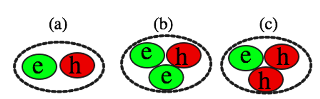
Figure 1: (a) An exciton X is a bound electron-hole pair. (b) A negative trion is a negatively charged exciton X^-. (c) A positive trion is a positively charged exciton X⁺.

Generally, the hole effective mass in semiconductors is larger than the electron effective mass because valence bands show weaker energy dispersion, and often the electron-hole mass ratio $\sigma$ lies in the range $0.01<\sigma<1$. Since the Coulomb interaction is symmetric in terms of particle charge, the binding energy of a negative trion with electron-hole mass ratio $\sigma$ is equal to the binding energy of a positive trion with electron-hole mass ratio $1/\sigma$. In fact, it is often more convenient to show the binding energy of a trion in terms of the rescaled mass ratio $x=\sigma/(1+\sigma)\in[0,1]$ rather than $\sigma\in[0,\infty)$. The binding energy of a negative trion with rescaled mass ratio $x$ is equal to the binding energy of a positive trion with rescaled mass ratio $1-x$.

DMC binding energies of negative and positive trions at different mass ratios $\sigma$ are listed in Appendix B, together with previous theoretical data where available. The binding energy reaches its maximum value for two heavy holes and one light electron ($\sigma=0$) or equivalently, two heavy electrons and one light hole ($\sigma\to\infty$).

In the case $\sigma\to 0$ ($m_{\text{e}}\ll m_{\text{h}}$), we have an X⁺ consisting of a light electron moving in the field of two slowly moving heavy holes, and the BO approximation can be applied to the Hamiltonian of Eq. (2) to separate the electron’s contribution to the total energy from the holes’ contributions. Let $R_{\text{eq}}$ be the position of the minimum of the BO potential energy between two heavy holes; then the BO potential energy at distance $r$ near $R_{\text{eq}}$ can be expanded as a Taylor series:

$$U_{\text{hh}}(r) = U_{\text{hh}}(R_{\text{eq}})+\frac{1}{2}U_{\text{hh}}^{\prime\prime}(R_{\text{eq}}){(r-R_{\text{eq}})}^{2}+\dots.$$ (14)

$$\equiv U_{\text{hh}}(R_{\text{eq}})+\frac{1}{2}\mu_{\text{hh}}\omega^{2}{(r-R_{\text{eq}})}^{2}.$$

The hole-hole reduced mass in e.u. is $\mu_{\text{hh}}=m_{\text{h}}/2=(1+1/\sigma)/2=1/(2x)$. Hence the vibrational frequency $\omega$ is

$$\omega=\sqrt{2U_{\text{hh}}^{\prime\prime}(R_{\text{eq}})\,x}.$$ (15)

From Eq. (15), the ground state energy of an X⁺ in the harmonic approximation is

$$E\approx U_{\text{hh}}(R_{\text{eq}})+\frac{1}{2}\omega=U_{\text{hh}}(R_{\text{eq}})+\frac{1}{2}\sqrt{{2U_{\text{hh}}^{\prime\prime}(R_{\text{eq}})x}}.$$ (16)

Thus the energy and hence binding energy of a positive trion increases as $\sqrt{x}$ at small $x$ (and by charge symmetry, the energy of a negative trion goes as $\sqrt{1-x}$ near $x=1$). Equation (16) suggests that a suitable fitting function for the binding energy of a negative trion is a Padé function in powers of $\sqrt{1-x}$:

$$E_{\text{X}^{-}}^{\text{B}}=\frac{\sum_{i=0}^{3}a_{i}{(1-x)}^{i/2}}{1+\sum_{j=1}^{3}b_{j}{(1-x)}^{j/2}},$$ (17)

where the values of the fitting parameters $\{a_{i}\}$ and $\{b_{j}\}$ are presented in Table 2. In Fig. 2 the formula in Eq. (17) is plotted against $x$ and compared with the original DMC data. The summed square of deviations (SSE) from the DMC data is $8.37\times 10^{-10}$ e.u., with a root-mean-square error (RMSE) of $7.128\times 10^{-6}$ e.u. Equation (17) also describes positive trions, provided $1-x$ is replaced by $x$.

Table 2: Fitted parameters in Eq. (17) for negative trion binding energies.

Parameter	Value (e.u.)
$a_{0}$	$0.10259977858492200$
$a_{1}$	$-0.19032032332604387$
$a_{2}$	$0.12107317507399042$
$a_{3}$	$-0.013040190842318337$
$b_{1}$	$0.34760392556048214$
$b_{2}$	$-0.20820698951970068$
$b_{3}$	$-0.40782706820695203$

Figure 2: DMC binding energies of negative trions against rescaled mass ratio $x=\sigma/(1+\sigma)$. The solid line shows the fit of Eq. (17).

Equation (17) enables us to predict the binding energy of a trion in a semiconductor in units of exciton Hartree given the electron-hole mass ratio. If we also know the actual electron and hole masses and permittivity, we can evaluate the exciton Hartree and hence find the binding energy in real units. In Table 3 we present examples of predicted binding energies of negative and positive trions using Eq. (17) for a range of technologically important semiconductors. In each case, the positive trion forms a stronger bound state than the negative trion. This appears to contradict the finding of Ref. [31], obtained by solving the Faddeev equations within the effective mass approximation, that a positive trion is unbound for semiconductors such as GaAs. In each case, DMC predicts the trion binding energy to be an order of magnitude smaller than the corresponding exciton binding energy. Therefore, one expects the exciton peak to hide the trion peak in each case. Also, biexciton peaks may be difficult to observe in experiments because the sub-meV binding energies are often less than experimental uncertainties. In the following sections, we will demonstrate another important application of our study in the field of atomic and molecular physics.

Table 3: Predicted binding energies of negative and positive trions (X^-) and biexcitons (X₂) in bulk semiconductors, using Eqs. (17) and (28), respectively, to interpolate our DMC data. The material parameters are shown in Table 1, while the fitting parameters in the interpolation formulas are given in Tables 2 and 8.

Crystal	$E_{\text{X}^{-}}^{\text{B}}$ (meV)	$E_{\text{X}^{+}}^{\text{B}}$ (meV)	$E_{\text{X}_{2}}^{\text{B}}$ (meV)
GaAs	$0.23910(3)$	$0.46066(4)$	$0.67338(2)$
	$0.5$
InAs	$0.065198(6)$	$0.15279(1)$	$0.238160(6)$
InSb	$0.069477(6)$	$0.15356(1)$	$0.235254(6)$
InP	$0.32245(4)$	$0.54338(5)$	$0.75443(3)$
Si	$0.77530(9)$	$0.97733(9)$	$1.24781(9)$
Ge	$0.20753(2)$	$0.29744(3)$	$0.38983(3)$

III.2.2 Mass effects in anions and molecular cations of hydrogen isotopes

Molecular cations of hydrogen isotopes (i.e., H${}_{2}^{+}$, D${}_{2}^{+}$, and T${}_{2}^{+}$) are effectively trions consisting of two extremely heavy “holes” (the nuclei) and one light electron. The binding energy of such a cation is the energy required to dissociate the system into a neutral atom and a single nucleus. On the other hand, atomic anions such as H^-, D^-, and T^- can be viewed as negative trions consisting of an extremely heavy “hole” and two light electrons. For these anions, the binding energy is the energy needed to separate an electron to infinite distance from the neutral atom and is equal to the electron affinity of the neutral atom.

We performed DMC simulations of these ions and we report the resulting total energies and binding energies in Table 4. We take the proton mass, deuteron mass, and triton mass to be $m_{\text{p}^{+}}=1836.152673440001$ a.u., $m_{\text{d}^{+}}=3670.482967853717$ a.u., and $m_{\text{t}^{+}}=5496.921535729647$ a.u., respectively [40]. The energy required to separate an electron from a hydrogen anion slightly increases with isotope mass, as expected from Fig. 2, and the corresponding energy approaches the $\sigma=0$ limit of a negatively charged trion. The same trend is observed for Ps^- and Mu^- (a bound state of an antimuon and two electrons), while the calculated values are in good agreement with the available experimental data.

Table 4: Ground-state total energy and binding energy of various ions obtained by DMC and compared with previous (experimental) works, where possible. d⁺ and t⁺ denote a deuteron and a triton, respectively.

Ion	Total energy (e.u.)			Binding energy (eV)
	DMC	Eq. (17)	Prev. works	DMC	Eq. (17)	Exp.
Ps- (e-e-e+)	$-0.52401(1)$	$-0.524009(2)$	$0.524010$	$0.3267(1)$	$0.32666(3)$	$0.33$
Mu- (e-e${}^{-}\mu^{+}$)	$-0.52759(5)$	$-0.527607(3)$		$0.747(1)$	$0.74761(8)$	$0.75$
H- (e-e-p+)	$-0.52762(7)$	$-0.527748(4)$		$0.751(2)$	$0.7547(1)$	$0.754$
D- (e-e-d+)	$-0.527742(4)$	$-0.527757(4)$		$0.7547(1)$	$0.7551(1)$	$0.755$15
T- (e-e-t+)	$-0.527744(3)$	$-0.527760(4)$		$0.75482(8)$	$0.7553(1)$
Mu${}_{2}^{+}$ (e${}^{-}\mu^{+}\mu^{+}$)	$-0.587951(2)$	$-0.58795(2)$		$2.38175(5)$	$2.3817(5)$
H${}_{2}^{+}$ (e-p+p+)	$-0.5974636(7)$	$-0.59745(1)$	$-0.60263461$ $-0.597464275221235$	$2.65068(2)$	$2.6503(3)$	$2.651$
D${}_{2}^{+}$ (e-d+d+)	$-0.59893(3)$	$-0.59893(1)$		$2.6913(8)$	$2.6913(3)$	$2.691$18
T${}_{2}^{+}$ (e-t+t+)	$-0.59956(5)$	$-0.59959(1)$		$2.709(1)$	$2.7095(3)$
X+ (e-h+h+), with $\sigma=0$	$-0.60265(2)$	$-0.60260(1)$	$-0.6025$	$2.7933(5)$	$2.79189(3)$

Similarly, DMC predicts a slight increase in binding energy with mass ratio for the three molecular cations of hydrogen isotopes, as seen in Table 4. The corresponding values approach the $\sigma=0$ limit for a positively charged trion, so that the heavier isotope T${}_{2}^{+}$ has a 3% larger binding energy than the lighter isotope H${}_{2}^{+}$.

For comparison, we also show the total energy and binding energy of the hydrogen ions calculated using Eq. (17) in Table 4. There is excellent agreement between the DMC results and Eq. (17). Consequently, knowing the electron-hole mass ratio, Eq. (17) can be used to predict the total energy and binding energy of either a trion in an isotropic semiconductor or a Coulomb complex in free space.

III.2.3 BO potential energy curve

The extreme electron-hole mass ratio of $\sigma=0$ is very important in atomic and molecular physics. The resulting BO potential allows us to compute important spectroscopic data. We calculated the BO potential energy curve as a function of hole-hole separation by solving the Schrödinger equation for a single electron in the presence of two fixed holes using DMC. We selected a wide range of hole-hole distances, between 1.4 and 3.5 a.u. DMC total energies for each hole-hole separation are given in Appendix C.1. The interaction between nuclei in a diatomic molecule or ion is often described by a Morse potential. The Morse potential can qualitatively describe the BO potential at very short and very large separations, as shown in Appendix C.2. However, because the Morse potential shows a significant deviation from the DMC data near the equilibrium separation, the resulting spectroscopic data based on the Morse model disagree with experiments. Instead, we found that a degree-six polynomial

$$U_{\text{hh}}(r)=\sum_{i=0}^{6}p_{i}r^{i},$$ (18)

fits our DMC data well near the equilibrium separation, as seen in Fig. 3. The SSE and RMSE of the fit are $1.061\times 10^{-8}$ and $3.434\times 10^{-5}$ a.u, respectively, and the maximum fractional deviation of the fitted function from the DMC data is less than 0.007%. The fitted coefficients $\{p_{i}\}$ are given in Appendix C.1.

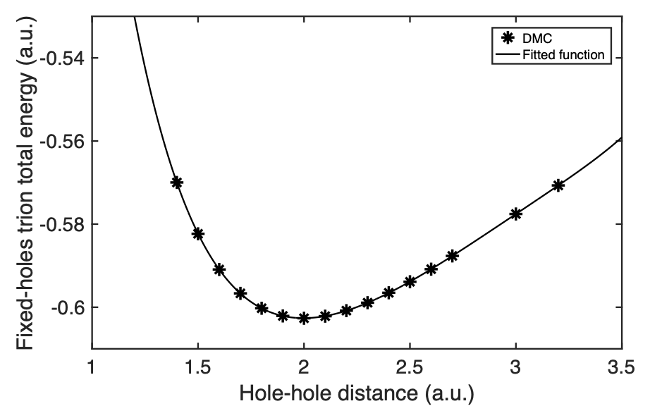
Figure 3: DMC BO potential energy, i.e., DMC total energy of a positive trion in the infinite mass limit of two heavy holes and one light electron ($\sigma=0$) against the hole-hole distance. The solid curve shows a fit of Eq. (18) to the DMC data.

For infinite hole mass, the electron-hole reduced mass is $\mu=m_{\text{e}}$, and assuming that $\epsilon_{\text{r}}=\epsilon_{0}$ (i.e., the complex is in free space), the exciton Bohr radius and exciton Hartree energy are equal to the atomic Bohr radius and Hartree energy (1 e.u.${}=1$ a.u.).

From Eq. (18) the minimum energy of a positive charged trion in the fixed hole limit occurs at $R_{\text{eq}}=1.9970(5)$ e.u., which agrees well with the prediction of Schaad et al., who used Burrau’s method to separate the Schrödinger equation for the single electron in H${}_{2}^{+}$ in confocal elliptical coordinates [45, 49]: see Table 5.

In another, more precise approach, we have calculated the mean nucleus-nucleus distance of the molecular hydrogen cation from the radial distribution function (RDF) $4\pi r^{2}g_{\text{hh}}(r)$ obtained using QMC calculations for the exact mass ratio, as shown in Fig. 4. The position of the peak in the hole-hole RDF gives the most likely nucleus-nucleus distance for each isotope. The mean nucleus-nucleus distance or bond length between two nuclei can be evaluated as $\langle r_{\text{hh}}\rangle=\int_{0}^{\infty}4\pi r^{2}g_{\text{hh}}(r)\,r\,dr$. DMC predicts a slight increase in the bond length of the system when nuclear dynamics are considered; see Table 5. Also, a slightly larger equilibrium nucleus-nucleus distance for lighter isotopes is obtained. These results are in good agreement with previous data when nuclear dynamics are included in the calculations [50]. In addition, the maximum of the RDF increases with the nuclear mass as we approach the static-nucleus limit.

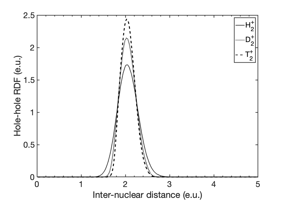
Figure 4: Nucleus-nucleus RDF $4\pi r^{2}g_{\text{hh}}(r)$ for three dihydrogen cations (H${}_{2}^{+}$, D${}_{2}^{+}$, and T${}_{2}^{+}$) versus the nucleus-nucleus distance.

Table 5: Adiabatic equilibrium nucleus-nucleus distance $R_{\text{eq}}$, nonadiabatic mean nucleus-nucleus and electron-nucleus distances $\langle r_{\text{hh}}\rangle$ and $\langle r_{\text{eh}}\rangle$, DMC zero-point energy (ZPE), difference $\Delta E_{\text{Z}}$ between the exact ZPE and the harmonic approximation $\omega_{\text{e}}/2$ to the ZPE, and spectroscopic constants of dihydrogen cations. Results are from the present work, except where citations are given.

Ion	$R_{\text{eq}}$ (a.u.)	$\langle r_{\text{hh}}\rangle$ (a.u.)	$\langle r_{\text{eh}}\rangle$ (a.u.)	$\sigma_{\text{hh}}$ (a.u.)	ZPE (eV)	$\Delta E_{\text{Z}}$ (meV)	$\omega_{\text{e}}$ (cm-1)	$\omega_{\text{e}}x_{\text{e}}$ (cm-1)	$\alpha_{\text{e}}$ (cm-1)	$B_{\text{e}}$ (cm-1)
H${}_{2}^{+}$	$1.9970(5)$ $1.9972(1)$ $2.0$	$2.063(9)$ $2.075(2)$ $2.06403(7)$	$1.69(3)$	$0.231(9)$	$0.1500(5)$	$6.0(7)$	$2323(4)$ $2315.3(6)$21 $2321$	$68(4)$ $67.3(2)$21 $66.2$24	$1.67(3)$ $1.600(3)$21 $1.68$24	$29.97$ $29.9626(2)$21 $30.2$24
D${}_{2}^{+}$	$1.9970(5)$ $1.9972(1)$20 $2.0$21	$2.059(9)$	$1.69(3)$	$0.180(9)$	$0.106(1)$	$4(1)$	$1643(3)$ $1577.3$	$34(2)$	$0.59(1)$ $0.560$25	$14.99$ $15.061$25
T${}_{2}^{+}$	$1.9970(5)$ $1.9972(1)$20	$2.061(9)$	$1.69(2)$	$0.159(9)$	$0.087(1)$	$4(1)$	$1343(2)$	$23(1)$	$0.322(6)$	$10.01$

The nucleus-nucleus spatial width of the lighter isotope H${}_{2}^{+}$ is slightly larger than the two others and shows a slight asymmetry, demonstrating that anharmonicity effects are more important in H${}_{2}^{+}$ than D${}_{2}^{+}$ or T${}_{2}^{+}$. The width of the RDF is quantified by the standard deviation $\sigma_{\text{hh}}=\sqrt{\left\langle r_{\text{hh}}^{2}\right\rangle-\left\langle r_{\text{hh}}\right\rangle^{2}}$. The standard deviation for H${}_{2}^{+}$ is $0.231(9)$ a.u. and it decreases for the more massive isotopes D${}_{2}^{+}$ and T${}_{2}^{+}$, as seen in Table 5. A previous path integral Monte Carlo study indicated a broadening of $0.539(1)$ a.u. and $0.454(1)$ a.u. at half maximum of RDF digram for H${}_{2}^{+}$ and D${}_{2}^{+}$, respectively [50]. On the other hand, as seen in Fig. 5, isotope mass does not strongly influence the electron-nucleus coupling, and we obtained three very similar $g_{\text{eh}}(r)$ curves, as implied by the BO approximation. Figure 5 also shows that $g_{\text{eh}}(r)$ falls off approximately exponentially with distance, with the associated lengthscale being $0.58(1)$ e.u.

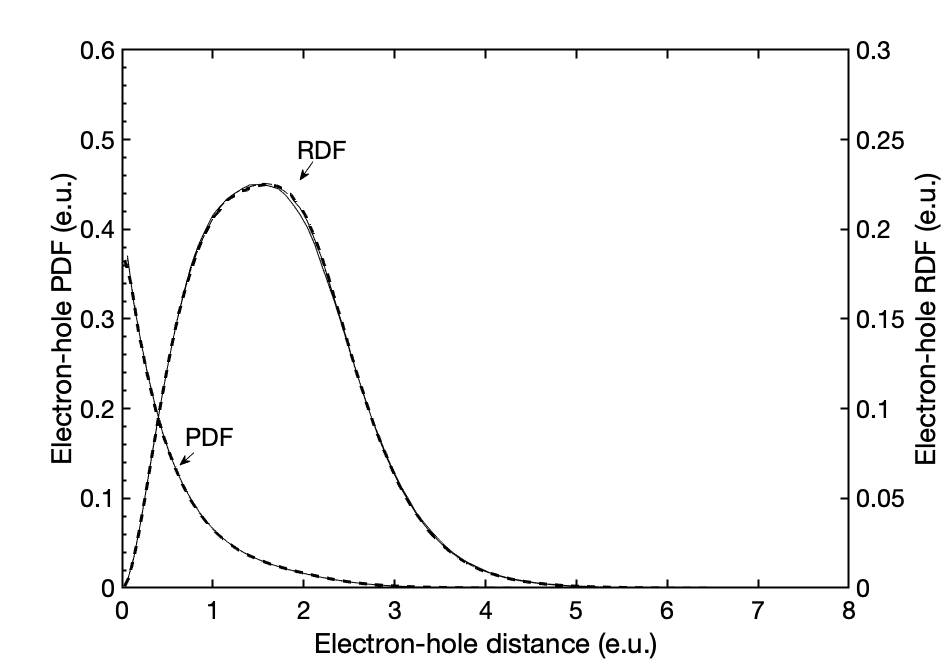
Figure 5: Electron-nucleus PDF $g_{\text{eh}}(r)$ and the corresponding RDF $4\pi r^{2}g_{\text{eh}}(r)$ in three dihydrogen cations (H${}_{2}^{+}$, D${}_{2}^{+}$, and T${}_{2}^{+}$) versus the electron-nucleus distance. The curves for the different ions are almost on top of each other.

III.2.4 Spectroscopic constants

For a given electronic state, the spectrum of the atomic system is determined by the corresponding vibrational and rotational levels. We applied the BO potential energy curve described by Eq. (18) to evaluate the contribution of rovibrational motion to the total energy by evaluating the spectroscopic constants of H${}_{2}^{+}$ isotopes from a Dunham polynomial [16]:

$$E_{nJ} = E_{00}+\omega_{\text{e}}\left(n+\frac{1}{2}\right)-\omega_{\text{e}}x_{\text{e}}{\left(n+\frac{1}{2}\right)}^{2}$$

$${}+B_{\text{e}}J(J+1)-\alpha_{\text{e}}J(J+1)\left(n+\frac{1}{2}\right)+\ldots,$$

where $E_{00}=U_{\text{hh}}(R_{\text{eq}})$ is the minimum of the BO potential, $\omega_{\text{e}}$ is the harmonic vibration frequency about the minimum of the BO potential, and $n=0,1,2,\ldots$ is the vibrational quantum number. $\omega_{\text{e}}x_{\text{e}}$ describes the effects of anharmonicity in the BO potential. $B_{\text{e}}J(J+1)$ is the angular kinetic energy and $J=0,1,2,\ldots$ is the rotational quantum number. $\alpha_{\text{e}}$ describes the strength of rovibrational coupling. In an adiabatic approach, we have used the energy function introduced by Eq. (18) at the equilibrium nucleus-nucleus distance within the BO approximation to calculate the spectroscopic constants of the H${}_{2}^{+}$ isotopes as [16]

$$B_{\text{e}} = \frac{1}{2\mu_{\text{hh}}r^{2}}$$ (20)

$$\omega_{\text{e}} = {\left(\frac{1}{\mu_{\text{hh}}}\frac{d^{2}U_{\text{hh}}}{dr^{2}}\right)}^{1/2}$$ (21)

$$\omega_{\text{e}}x_{\text{e}} = \frac{1}{48\mu_{\text{hh}}}\left[5{\left(\frac{\frac{d^{3}U_{\text{hh}}}{dr^{3}}}{\frac{d^{2}U_{\text{hh}}}{dr^{2}}}\right)}^{2}-3\frac{\frac{d^{4}U_{\text{hh}}}{dr^{4}}}{\frac{d^{2}U_{\text{hh}}}{dr^{2}}}\right]$$ (22)

$$\alpha_{\text{e}} = -\frac{6B_{\text{e}}^{2}}{\omega_{\text{e}}}\left(\frac{R}{3}\frac{d^{3}U_{\text{hh}}/dr^{3}}{d^{2}U_{\text{hh}}/dr^{2}}+1\right).$$ (23)

Here, $r$ is the nucleus-nucleus distance and $\mu_{\text{hh}}=m_{\text{h}}/2$ is the reduced mass of the two nuclei. Our results are presented in Table 5 and compared with the available data in the literature.

The spectroscopic parameters given in Eqs. (20)–(23) can be evaluated either at the equilibrium separation $r=R_{\text{eq}}$ or by taking their expectation values with respect to the nucleus-nucleus PDF. The results did not change significantly when the spectroscopic parameters were calculated by taking their expectation value with respect to the PDF instead of calculating the parameters at the adiabatic equilibrium distance $R_{\text{eq}}$, and hence our reported results just used $r=R_{\text{eq}}$. In Table 4 we report the exact vibrational ZPE of each dihydrogen cation as the difference between the ground-state energy and the minimum total energy of a heavy-hole positive trion X⁺ ($\sigma=0$). Comparing the ZPEs of these three isotopes with the harmonic part of their vibrational energy $\omega_{\text{e}}/2$ shows that anharmonicity makes a larger contribution to the ZPE of H${}_{2}^{+}$ than in the other two isotopes, as can be seen in Table 5. As shown in Table 5, the ZPE falls off as the nuclear mass increases. Zero-point fluctuations are responsible for the broadening of the nucleus-nucleus RDF in Fig. 4 at temperature $T=0$.

Electron-positron contact pair densities (which determine annihilation rates) are given in Table 6.

Table 6: VMC-DMC extrapolated estimates of the opposite-spin electron-positron contact pair density $g_{\text{eh}}({\bf 0})/2$ in some positronic ions and molecules. The analytic result for Ps is shown for comparison. The error bars quantify the uncertainty due to VMC and DMC simulation, but not errors due to the form and optimization of the trial wave function.

Complex	$g_{\text{eh}}({\bf 0})/2$ (a.u.)
Ps	$1/(16\pi)$
Ps-	$0.020709(9)$
Ps2	$0.04427(1)$
PsH	$0.02465(2)$
PsD	$0.02455(1)$
PsT	$0.02457(1)$

III.2.5 Accuracy of BO and harmonic approximations

Equation (18) gives the BO potential energy surface, which only depends on the hole-hole distance $r_{\text{hh}}$. Transforming to the hole-hole center of mass and difference coordinates, as done for electron-hole relative motion in an exciton in Eq. (4), the nuclear part of the Schrödinger equation within the BO approximation is

$$\left[-\frac{1}{2\mu_{\text{hh}}}\nabla_{\text{hh}}^{2}+U_{\text{hh}}(r_{\text{hh}})\right]\psi_{\text{hh}}({\bf r}_{\text{hh}})=E_{\text{BO}}\psi_{\text{hh}}({\bf r}_{\text{hh}}),$$ (24)

where $\psi_{\text{hh}}({\bf r}_{\text{hh}})$ is the hole-hole wave function. $E_{\text{BO}}$ represents the total energy of the system within the (fully anharmonic) BO approximation. In a spherically symmetric system, the wave function only depends on the hole-hole separation $r_{\text{hh}}$. Consequently, Eq. (24) reduces to a one-dimensional Schrödinger equation

$$-\frac{1}{2\mu_{\text{hh}}}\left(\frac{d^{2}}{dr_{\text{hh}}^{2}}+\frac{2}{r}\dfrac{d}{dr_{\text{hh}}}\right)\psi_{\text{hh}}(r_{\text{hh}})+U_{\text{hh}}(r_{\text{hh}})\psi_{\text{hh}}(r_{\text{hh}})$$

$${}=E_{\text{BO}}\psi_{\text{hh}}(r_{\text{hh}}).$$ (25)

We have employed the shooting method with the initial condition $\psi_{\text{hh}}(0)=0$ and $\frac{d\psi_{\text{hh}}(r_{\text{hh}})}{dr_{\text{hh}}}=0$ at large separation to solve Eq. (25) numerically for the H${}_{2}^{+}$ cation. In Table 7 we compare (i) the exact nonrelativistic energy obtained using DMC for all the constituent particles, (ii) the energy within the fully anharmonic BO approximation obtained using the shooting method, and (iii) the harmonic approximation within the BO framework, in which the total energy is

$$E_{\text{BO+Harm.}}=U_{\text{hh}}(R_{\text{eq}})+\frac{\omega_{\text{e}}}{2}.$$ (26)

From the data in Table 7, the BO energies are about 0.0003–0.0005 a.u. lower than the DMC-calculated exact energies. In Fig. 6 the probability density $|\psi_{\text{hh}}(r_{\text{hh}})|^{2}$ within the BO approximation is compared with both the DMC hole-hole RDF and the ground state probability density in the harmonic approximation, ${(\mu_{\text{hh}}\omega_{\text{e}}/\pi)}^{1/2}e^{-\mu_{\text{hh}}\omega_{\text{e}}{(r_{\text{hh}}-R_{\text{eq}})}^{2}}$, where $R_{\text{eq}}$ and $\omega_{\text{e}}$ are taken from Table 5. The BO fully anharmonic hole-hole RDF, shown in Fig. 6, is in slightly better agreement with the DMC hole-hole RDF than is the BO harmonic approximation, especially for the tails of the RDF. On the other hand, surprisingly, the harmonic approximation gives a more accurate ground-state total energy than the fully anharmonic BO approximation in comparison with the DMC simulation of all the particles. The likely reason for this pathological behavior of the BO approximation is that, at the level of accuracy at which we are working, the ambiguity in the mass of the heavy particles is significant: should some fraction of the electron mass be included in $\mu_{\text{hh}}$?

Table 7: Total energy of the molecular hydrogen cation H${}_{2}^{+}$ and dihydrogen H₂ from three different approaches: (i) the exact nonrelativistic solution $E$ obtained using DMC, (ii) the BO approximation $E_{\text{BO}}$, (iii) the BO and harmonic approximations $E_{\text{BO+Harm.}}$

Complex	$E$ (a.u.)	$E_{\text{BO}}$ (a.u.)	$E_{\text{BO+Harm.}}$ (a.u.)
H${}_{2}^{+}$	$-0.5971384(7)$	$-0.59738903$	$-0.597340(7)$
H2	$-1.164015(8)$	$-1.1645088$	$-1.16441(2)$

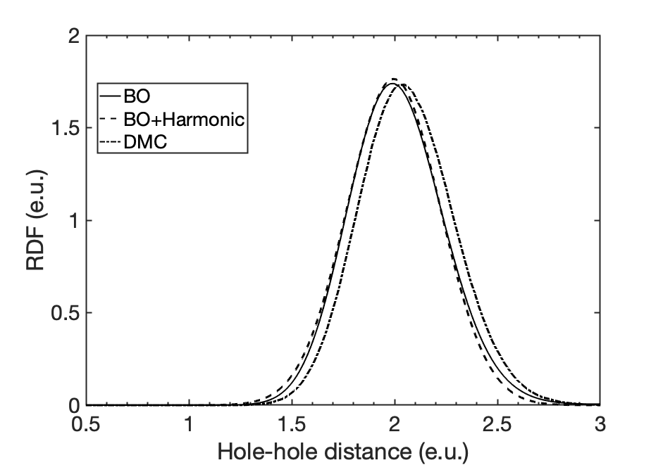
Figure 6: Proton-proton RDF in a hydrogen molecular cation obtained using the three different approaches listed in the caption of Table 7.

III.3 Biexcitons

III.3.1 Binding energies

The binding energy of a biexciton is the energy required to decompose it into its two constituent excitons:

$$E_{\text{X}_{2}}^{\text{B}}=2E_{\text{X}}-E_{\text{X}_{2}},$$ (27)

where $E_{\text{X}_{2}}$ is the ground state total energy of the biexciton.

As we have done for a trion, in the limit of two heavy holes, we can employ the BO approximation and separate the vibrational contribution of heavy holes to the total energy from the electronic contribution. The derivation of Eq. (16) is exactly the same for a biexciton as for a positive trion, again leading to the conclusion that the binding energy must go as $\sqrt{x}$ at small $x$. However, unlike a trion, the binding energy must be unchanged under the exchange of electrons and holes (i.e., $m_{\text{e}}\leftrightarrow m_{\text{h}}$ or, equivalently, $\sigma\leftrightarrow 1/\sigma$ or $x\leftrightarrow 1-x$). This suggests that a suitable fitting function for the binding energy of a biexciton should be a symmetric polynomial in $\sqrt{x}$ and $\sqrt{1-x}$. We found the DMC binding energy data to be well fitted by

$$E_{\text{X}_{2}}^{\text{B}}=\sum_{i=0}^{4}c_{i}{[x(1-x)]}^{i/2}.$$ (28)

The fitting parameters $\{c_{i}\}$ are presented in Table 8 and the fitted curve is plotted along with the raw data in Fig. 7. The DMC total energies are listed in Appendix B. The SSE and RMSE are $2.249\times 10^{-9}$ e.u. and $1.224\times 10^{-5}$ e.u., respectively.

Table 8: Fitted parameters in Eq. (28) for biexciton binding energies.

Parameter	Value (e.u.)
$c_{0}$	$0.17438546591410939$
$c_{1}$	$-0.42831856512902888$
$c_{2}$	$0.38685906773221207$
$c_{3}$	$-0.26511242810730029$
$c_{4}$	$0.13132632976660738$

Figure 7: DMC binding energies of biexcitons against rescaled mass ratio $x=\sigma/(1+\sigma)$. The solid line shows the fit of Eq. (28).

Using Eq. (28), we predict the biexciton binding energy in various semiconductors in Table 3. In all cases, the biexciton binding energies are larger than the trion binding energies, but are of the same order of magnitude.

III.3.2 Mass effects in molecular hydrogen isotopes

An H₂ molecule consists of two protons and two electrons and hence resembles a biexciton with heavy holes. Likewise, a dimuonium molecule Mu₂ is formed by the electrostatic interaction between two electrons and two antimuons. The binding energy of such a molecule is defined as the energy required to dissociate the molecule into two isolated atoms. The DMC ground state total energies and binding energies of dimuonium and the molecular hydrogen isotopes H₂, D₂, and T₂ are given in Table 9. The DMC-calculated total energies are in excellent agreement with previous quantum electrodynamics predictions [54], confirming that the molecules are well described by nonrelativistic quantum mechanics. Indeed, the DMC binding energies retrieve the experimental outcomes and show that the binding energy increases with nuclear mass. As can be seen in Table 9, Eq. (28) predicts the binding energies of the three molecular hydrogen isotopes in good agreement with both the raw DMC data and experimental results.

Table 9: As Table 4, but for neutral dihydrogen-like molecules. Raw data in Ref. 54 are given in a.u.; for easy comparison with DMC results, we converted them to e.u. and rounded them to a smaller number of digits.

Molecule	Total energy (e.u)			Binding energy (eV)
	DMC	Eq. (28)	Prev. works	DMC	Eq. (28)	Exp.
Ps2 (e-e-e+e+)	$-1.032009(3)$	$-1.032010(3)$	$-1.03196$	$0.43550(4)$	$0.43552(4)$
Mu2 (e-e${}^{-}\mu^{+}\mu^{+}$)	$-1.1465(1)$	$-1.14651(1)$		$3.967(3)$	$3.9676(3)$
H2 (e-e-p+p+)	$-1.164649(8)$	$-1.16460(1)$	$-1.164659$	$4.4779(2)$	$4.4766(3)$	$4.478$
D2 (e-e-d+d+)	$-1.167482(2)$	$-1.16742(1)$	$-1.167487$27	$4.55618(5)$	$4.5545(3)$	$4.556$28
T2 (e-e-t+t+)	$-1.168749(3)$	$-1.16868(1)$	$-1.168748$27	$4.59106(8)$	$4.5892(3)$	$4.586$27
X2 (e-e-h+h+), with $\sigma=0$	$-1.17443(3)$	$-1.17439(1)$		$4.7465(8)$	$4.7454(3)$

III.3.3 BO potential energy curve

As with molecular cations, the BO potential energy curve provides important information about the nuclear motion around the equilibrium separation. We performed a series of DMC simulations of two electrons in the presence of two fixed holes at different hole-hole distances, between 0.8 and 1.8 a.u. The results are shown in Appendix B and compared with the available previous data. We found that a polynomial of degree eight,

$$U_{\text{hh}}(r)=\sum_{i=0}^{8}p_{i}r^{i},$$ (29)

fitted our data excellently, with the coefficients $\{p_{i}\}$ reported in Appendix C.1. The SSE and RMSE are $3.02\times 10^{-9}$ and $3.173\times 10^{-5}$ a.u., respectively. Figure 8 shows how well the curve given by Eq. (29) passes through the DMC data.

III.3.4 Spectroscopic constants

We have calculated the spectroscopic constants of molecular hydrogen from the potential energy curve given by Eq. (29), using Eqs. (20)–(23) evaluated at the equilibrium separation. The results are shown in Table 10. For comparison, the spectroscopic constants obtained from a Morse model are given in Appendix C.2. The adiabatic equilibrium nucleus-nucleus distance is $R_{\text{eq}}=1.4$ a.u., which agrees with a previous adiabatic VMC prediction [58]. Furthermore, we obtained the vibrational ZPE of these molecules by comparing adiabatic and nonadiabatic energies. Our spectroscopic constants are in good agreement with the available experiments, as seen in Table 10.

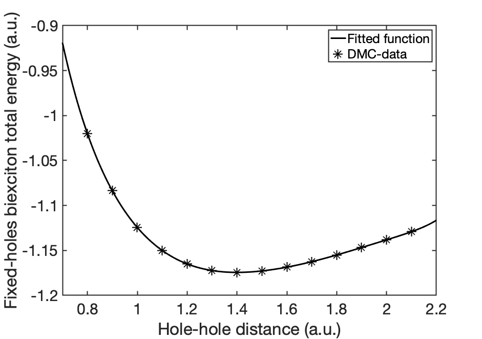
Figure 8: DMC BO potential energy, i.e., DMC total energy of a biexciton in the infinite mass limit of two heavy holes and two light electrons ($\sigma=0$) against the hole-hole distance. The solid curve shows a fit of Eq. (29) to the DMC data.

Table 10: As Table 5, but for neutral dihydrogen molecules.

Mol.	$R_{\text{eq}}$ (a.u.)	$\langle r_{\text{hh}}\rangle$ (a.u.)	$\langle r_{\text{eh}}\rangle$ (a.u.)	$\sigma_{\text{hh}}$ (a.u.)	ZPE (eV)	$\Delta E_{\text{Z}}$ (meV)	$\omega_{\text{e}}$ (cm-1)	$\omega_{\text{e}}x_{\text{e}}$ (cm-1)	$\alpha_{\text{e}}$ (cm-1)	$B_{\text{e}}$ (cm-1)
H2	$1.400(5)$ $1.4$ $1.401$	$1.44(2)$ $1.4193$	$1.57(6)$	$0.16(2)$	$0.2834(8)$ $0.270$	$10(1)$	$4400(10)$ $4401.213$32	$110(30)$ $121.336$32	$3.1(2)$ $3.0622$32	$60.984$ $60.853$32
D2	$1.400(5)$	$1.43(2)$ $1.4139$31	$1.57(4)$	$0.14(2)$	$0.1977(8)$ $0.1917$31	$4(1)$	$3120(10)$ $3115.5$32	$55(7)$ $61.82$32	$1.03(7)$ $1.0786$32	$30.50739(2)$ $30.4436$32
T2	$1.400(5)$	$1.43(2)$ $1.41146(4)$	$1.57(6)$	$0.13(2)$	$0.1604(8)$ $0.1569$	$2(1)$	$2547(8)$ $2546.4$34	$36(5)$ $41.23$34	$0.56(4)$ $0.5887$	$20.371$ $20.335$34

In Appendix C.2 we compare our model, given by Eq. (29), with the Morse potential. As in the case of trions, although a Morse potential behaves much better than Eq. (29) at large hole-hole separations, it does not match the DMC data so well in the vicinity of the equilibrium point.

Figure 9: Nucleus-nucleus RDF $4\pi r^{2}g_{\text{hh}}(r)$ for three dihydrogen molecules (H₂, D₂, and T₂) versus the nucleus-nucleus distance.

Figure 10: Electron-nucleus PDF $g_{\text{eh}}(r)$ and RDF $4\pi r^{2}g_{\text{eh}}(r)$ in three dihydrogen molecules (H₂, D₂, and T₂) versus the electron-nucleus distance.

Using the RDF results obtained from nonadiabatic QMC simulations of two electrons and two nuclei, we explore the effects of nuclear motion on the bond lengths of the molecular hydrogen isotopes. Our results show slight increases in bond length when nuclear dynamics are considered, bringing our results into agreement with the available experimental data, as shown in Table 10.

Figure 9 shows the nucleus-nucleus RDF for the three molecular hydrogen isotopes. As is the case for H${}_{2}^{+}$, the distribution of nucleus-nucleus distances in H₂ has a larger spatial broadening than in the more massive isotopes, as quantified by the standard deviation of the nucleus-nucleus distance reported in Table 10. Accordingly, the ZPE increases with electron-hole mass ratio $\sigma$, as seen in Table 10. The effects of anharmonicity are visible in Fig. 9 as an asymmetry in the RDF.

On the other hand, isotope mass does not influence the electron-nucleus coupling: the three molecules show the same electron-nucleus PDF curves in Fig. 10. Indeed, for all three molecules, the mean electron-nucleus distance $\langle r_{\text{eh}}\rangle$ is only slightly less than the mean electron-nucleus distance in the molecular cations.

The exact nonrelativistic energy of H₂, the energy within the BO approximation, and the energy within the harmonic approximation within the BO framework are shown in Table 7 and the corresponding RDFs are shown in Fig. 11. The mean separation obtained within exact DMC calculations for all four particles is greater than the equilibrium separation of the BO potential. As in the dihydrogen cation, the harmonic approximation appears to perform better than the fully anharmonic BO approximation.

Figure 11: Proton-proton RDF in a hydrogen molecule H₂ from three different approaches: BO approximation, BO+harmonic approximation, and the DMC solution to the four-particle problem.

III.4 Other Coulomb complexes: mixed hydrogenic molecules and cations; helium hydride; and positronic and muonic complexes

The DMC-calculated nonrelativistic ground-state total energies of a number of small Coulomb complexes are shown in Table 11. We take the masses of a proton (p⁺), deuteron (d⁺), triton (t⁺), helion (h²⁺), alpha particle ($\alpha^{2+}$), and muon ($\mu^{\pm}$) to be $m_{\text{p}^{+}}=1836.152673440001$ a.u., $m_{\text{d}^{+}}=3670.482967853717$ a.u., $m_{\text{t}^{+}}=5496.921535729647$ a.u., $m_{\text{h}^{2+}}=5495.885280115730$ a.u., $m_{\alpha^{2+}}=7294.299425443957$ a.u., and $m_{\mu^{\pm}}=206.7682830910218$ a.u., respectively [40]. With the exception of H${}_{3}^{+}$, the ground-state spatial wave function is nodeless in each case and hence DMC provides numerically exact solutions to the nonrelativistic Schrödinger equation. For H${}_{3}^{+}$ we treat the three protons as distinguishable particles. Many of these compounds play important roles in interstellar chemistry.

Table 11: DMC nonrelativistic ground-state total energies of various Coulomb complexes.

Complex	Total energy (a.u.)
	DMC	Prev. works
$\mu^{+}$H (e${}^{-}\mu^{+}$p+)	$-0.58990(2)$
$\mu^{+}$D (e${}^{-}\mu^{+}$d+)	$-0.59023(2)$
$\mu^{+}$T (e${}^{-}\mu^{+}$t+)	$-0.59028(3)$
HD (e-e-p+d+)	$-1.165472(7)$	$-1.16547192396366(5)$
HT (e-e-p+t+)	$-1.166027(9)$	$-1.16600203732867(6)$36
DT (e-e-d+t+)	$-1.16781(1)$	$-1.16781967343673(5)$36
HD+ (e-p+d+)	$-0.59790(4)$
HT+ (e-p+t+)	$-0.59817(1)$
DT+ (e-d+t+)	$-0.59915(2)$
3He${}_{2}^{2+}$ (e-e-h2+h2+	$-3.672410(7)$
3He 4He2+ (e-e-h${}^{2+}\alpha^{2+}$)	$-3.67302(1)$
4He${}_{2}^{2+}$ (e-e${}^{-}\alpha^{2+}\alpha^{2+}$)	$-3.67364(1)$
H${}_{3}^{+}$ (e-e-p+p+p+)	$-1.32344(1)$
H2D+ (e-e-p+p+d+)	$-1.325273(7)$
H2T+ (e-e-p+p+t+)	$-1.325985(9)$
HD${}_{2}^{+}$ (e-e-p+d+d+)	$-1.327270(9)$
HDT+ (e-e-p+d+t+)	$-1.328035(9)$
HT${}_{2}^{+}$ (e-e-p+t+t+)	$-1.328830(9)$
D${}_{3}^{+}$ (e-e-d+d+d+)	$-1.329399(9)$
D2T+ (e-e-d+d+t+)	$-1.330230(9)$
DT${}_{2}^{+}$ (e-e-d+t+t+)	$-1.331115(9)$
T${}_{3}^{+}$ (e-e-t+t+t+)	$-1.332040(9)$
3He (e-e-h2+)	$-2.9031670(7)$
4He (e-e${}^{-}\alpha^{2+}$)	$-2.9033053(7)$
3HeH+ (e-e-p+h2+)	$-2.970719(6)$
4HeH+ (e-e-p${}^{+}\alpha^{2+}$)	$-2.97107(1)$
3HeD+ (e-e-d+h2+)	$-2.972272(9)$
4HeD+ (e-e-d${}^{+}\alpha^{2+}$)	$-2.972691(7)$
3HeT+ (e-e-t+h2+)	$-2.972895(7)$
4HeT+ (e-e-t${}^{+}\alpha^{2+}$)	$-2.97335(1)$
PsH (e-e-e+p+)	$-0.78890(2)$
PsD (e-e-e+d+)	$-0.78904(3)$
PsT (e-e-e+t+)	$-0.78909(3)$

For the positronic compounds we report the contact pair density $g_{\text{eh}}({\bf 0})/2$ between spin-up electrons and the positron in Table 6. It is clear that isotope effects in the electron-positron annihilation rate in PsH, PsD, and PsT are small.

IV Conclusions

We report high-precision, statistically exact DMC calculations of the binding energies of three-dimensional excitonic complexes in terms of the electron-hole mass ratio. In particular, we have focused on three- and four-body complexes (trions and biexcitons) formed from distinguishable electrons and holes with isotropic effective masses and interacting via an isotropic $1/r$ Coulomb potential. Based on our DMC data, we obtained interpolation formulas for the binding energies of trions and biexcitons. These formulas can be applied to interpret experimental photoabsorption and photoluminescence spectra in 3D semiconductors. Furthermore, based on DMC calculations with small mass ratios, we have calculated the nonrelativistic binding energies of “real” three-, four- and five-particle Coulomb complexes, including hydrogen molecules and ions (with different isotopes), helium hydride cations, and small positronic and muonic complexes. Using QMC PDFs, we predict the nonadiabatic nucleus-nucleus distance, nuclear spatial distribution, and spectroscopic constants for hydrogen molecules and ions. Where comparison is possible, our nonrelativistic results are in good agreement with both experiments and previous theoretical results obtained within quantum electrodynamics.

We find reasonable agreement between the exact nonrelativistic total energy of H₂ and the total energy within the BO approximation. Interestingly, we find that the total energy evaluated within the BO approximation including all anharmonic effects is slightly less accurate than the total energy evaluated using the harmonic approximation to the BO potential. Similar conclusions are reached for H${}_{2}^{+}$. This shows that it cannot be guaranteed that the inclusion of vibrational anharmonicity within the BO framework improves the total energy of a molecule or crystal, especially when light atoms such as hydrogen are present.

An important conclusion of our work is that, at least for the small molecules that we have studied, QMC simulations in which the nuclei are treated as quantum particles on an equal footing with the electrons are no more difficult and only proportionately more expensive than calculations with fixed nuclei, provided that an appropriate vibrational Jastrow factor is used. This holds out the prospect that QMC calculations for larger systems with a full quantum treatment of nuclei could routinely be performed using Jastrow factors that are quadratic functions of the phonon normal coordinates.

Appendix A Extrapolation of DMC results to zero time step

Figures 12 and 13 show extrapolation of DMC energies to zero time step for the H${}_{2}^{+}$ ion and the H₂ molecule, respectively. In both figures the DMC energies at zero time step are obtained from two fits: (i) a quadratic function fitted to six time steps and (ii) a linear fit to two small time steps. The zero-time-step results are the same to within the statistical error bars.

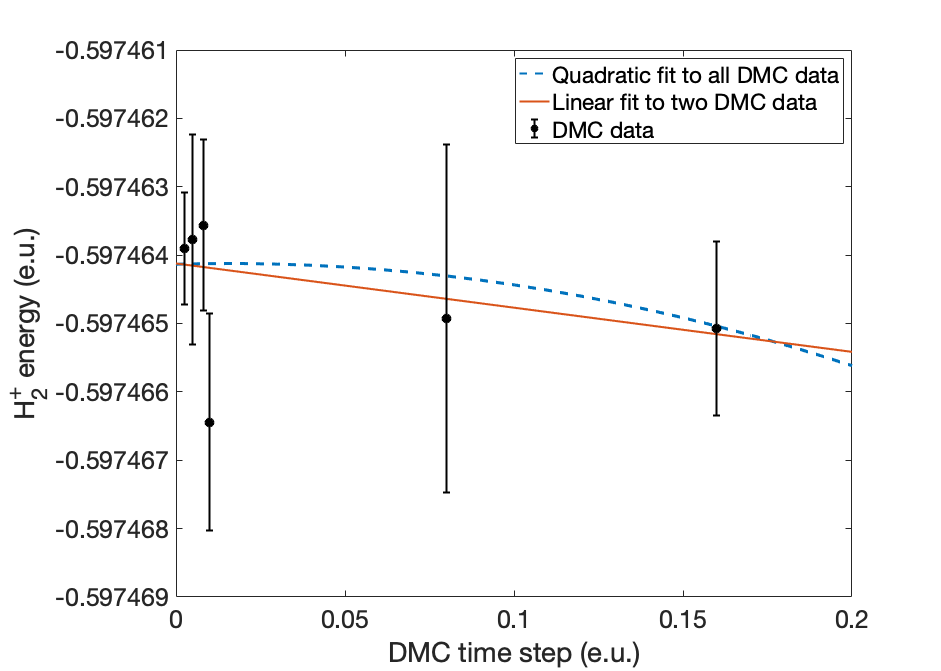
Figure 12: DMC total energy against time step for an H${}_{2}^{+}$ ion (a positive trion with a very small electron-hole mass ratio of $\sigma\approx 0.0005446$). A quadratic fit to the DMC energies at time steps of $0.0025$, $0.005$, $0.008$, $0.01$, $0.08$, and $0.16$ e.u. is shown as a dashed blue line. A linear fit to the DMC energies at two small time steps of $0.0025$ and $0.01$ e.u. is shown as a solid red line. The DMC energies extrapolated to zero time step using the quadratic and linear fits are $-0.5974637(4)$ and $-0.5974636(7)$ e.u., respectively.

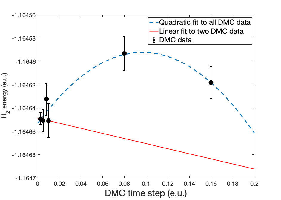
Figure 13: As Fig. 12, but for an H₂ molecule. The DMC energies extrapolated to zero time step using quadratic and linear fits are $-1.164653(5)$ and $-1.164649(8)$ e.u., respectively.

Appendix B DMC total energies for trions and biexcitons

The DMC energies of negative trions, positive trions, and biexcitons are reported in Tables 12, 13, and 14, respectively.

Table 12: DMC total energies of negative trions against mass ratio $\sigma$.

$\sigma$	Total energy (e.u.)
	DMC (pres. work)	Prev. works
0	$-0.527760(5)$	$-0.5282$ $-0.5275$
0.05	$-0.526318(4)$
0.10	$-0.524994(6)$
0.20	$-0.523792(4)$
0.32	$-0.522915(7)$
0.40	$-0.522653(6)$	$-0.5222$38
0.50	$-0.522550(6)$	$-0.5246$37
0.64	$-0.522737(8)$
0.70	$-0.522881(7)$	$-0.52275$38
0.80	$-0.523191(8)$
0.90	$-0.523599(8)$
1	$-0.52401(1)$	$-0.524$38
$\infty$	$-0.60261(2)$

Table 13: DMC total energies of positive trions against mass ratio $\sigma$.

$\sigma$	DMC total energy (e.u.)
0	$-0.60265(3)$
0.05	$-0.56283(3)$
0.10	$-0.551984(5)$
0.20	$-0.54094(1)$
0.32	$-0.534225(5)$
0.40	$-0.531452(5)$
0.50	$-0.529034(6)$
0.64	$-0.526793(7)$
0.70	$-0.52612(1)$
0.80	$-0.52521(2)$
0.90	$-0.524521(5)$
1	$-0.524002(5)$

Table 14: DMC total energy (in e.u.) of a biexciton X₂ against mass ratio $\sigma$.

$\sigma$	DMC total energy (e.u.)
$0$	$-1.17437(2)$
$0.04$	$-1.104619(7)$
$0.05$	$-1.098427(5)$
$0.08$	$-1.084599(4)$
$0.1$	$-1.07784(1)$
$0.2$	$-1.04545(2)$
$0.4$	$-1.04088(2)$
$0.5$	$-1.03715(2)$
$0.62$	$-1.034469(8$
$0.725$	$-1.033133(4)$
$0.8$	$-1.032556(4)$
$0.92$	$-1.03206(3)$
$1$	$-1.03203(2)$ $-1.0321(1)$
$1.6$	$-1.0344(2)$
$2.5$	$-1.04086(1)$
$4$	$-1.05136(1)$
$9$	$-1.074611(4)$
$20$	$-1.098425(5)$
$\infty$	$-1.17440(2)$

Appendix C Born-Oppenheimer potential curves

C.1 DMC energies and fits

DMC energies against hole-hole separation for positive trions and biexcitons are reported in Tables 15 and 16, respectively. The parameters in the polynomials [Eqs. (18) and (29)] fitted to the DMC BO data are reported in Tables 17 and 18, respectively.

Table 15: DMC total energy of a positive trion in the heavy hole limit ($\sigma=0$), i.e., the BO potential energy $U_{\text{hh}}$. In each calculation, the two holes are fixed with separation $r_{\text{hh}}$.

$r_{\text{hh}}$ (e.u.)	$U_{\text{hh}}$ (e.u.)
	DMC (pres. wk.)	VMC
$1.4$	$-0.56998(2)$	$-0.569983491(6)$
$1.5$	$-0.58233(2)$	$-0.582323174(5)$
$1.6$	$-0.59092(2)$	$-0.590937199(5)$
$1.7$	$-0.59672(2)$	$-0.596696250(4)$
$1.8$	$-0.60024(2)$	$-0.600253616(4)$
$1.9$	$-0.60209(2)$	$-0.602105768(3)$
$2$	$-0.60265(2)$	$-0.602634202(3)$
$2.1$	$-0.60215(2)$	$-0.602134935(3)$
$2.2$	$-0.60082(2)$	$-0.600839617(3)$
$2.3$	$-0.59891(2)$	$-0.598930879(3)$
$2.4$	$-0.59652(2)$	$-0.596553632(3)$
$2.5$	$-0.59381(2)$	$-0.593823505(2)$
$2.6$	$-0.59084(2)$	$-0.590833192(2)$
$2.7$	$-0.58765(2)$	$-$
$3.0$	$-0.57756(3)$	$-0.577562861(2)$
$3.2$	$-0.57069(2)$	$-$
$3.5$	$-0.56092(8)$	$-$

Table 16: DMC total energy of a biexciton in the heavy hole limit ($\sigma=0$), i.e., the BO potential energy $U_{\text{hh}}$. In each calculation, the two holes are fixed with separation $r_{\text{hh}}$.

$r_{\text{hh}}$ (e.u.)	$U_{\text{hh}}$ (e.u.)
	DMC (pres. wk.)	Prev. wk.
$0.2$	$2.1976(2)$	$2.197807(4)$
$0.8$	$-1.02007(2)$	$-1.020056(1)$
$0.9$	$-1.08362(2)$
$1$	$-1.12449(2)$	$-1.124539(2)$
$1.1$	$-1.15005(2)$
$1.2$	$-1.16488(2)$
$1.3$	$-1.17231(2)$
$1.4$	$-1.17445(3)$	$-1.174475(3)$
$1.5$	$-1.17280(3)$
$1.6$	$-1.16860(3)$
$1.7$	$-1.16244(3)$
$1.8$	$-1.15503(3)$	$-1.1550699(2)$
$1.9$	$-1.14683(3)$
$2$	$-1.13818(3)$
$2.1$	$-1.12917(3)$
$2.5$	$-1.0881(10)$

Table 17: Coefficients of the fitting function Eq. (18) for the BO potential of a positive trion, determined by fitting to the data in Table 15 in the range 1.4 a.u.${}\leq r_{\text{hh}}\leq 3.2$ a.u.

Parameter	Value (e.u.)
$p_{0}$	$1.0427824014296136$
$p_{1}$	$-3.3397706586457314$
$p_{2}$	$2.8588375211577741$
$p_{3}$	$-1.3365671624439441$
$p_{4}$	$0.36129754841667888$
$p_{5}$	$-0.053146452736184853$
$p_{6}$	$0.0033007257815276473$

Table 18: Coefficients of the fitting function Eq. (29) for the BO potential of a biexciton, determined by fitting to the data in Table 16 in the range 0.8 a.u.${}\leq r_{\text{hh}}\leq 1.9$ a.u.

Parameter	Value (e.u.)
$p_{0}$	$4.9372623192546792$
$p_{1}$	$-26.739727920240565$
$p_{2}$	$55.588815121898229$
$p_{3}$	$-70.359270025396583$
$p_{4}$	$57.928244487543246$
$p_{5}$	$-31.202873732362676$
$p_{6}$	$10.619660811375310$
$p_{7}$	$-2.0737318548490848$
$p_{8}$	$0.17711891075798453$

C.2 Comparison of polynomial and Morse potential fits to BO potential

A Morse interatomic potential is of the form

$$U_{\text{Morse}}(r)=D_{\text{eq}}\left[e^{-2a(r-R_{\text{eq}})}-2e^{-a(r-R_{\text{eq}})}\right],$$ (30)

where the equilibrium separation $R_{\text{eq}}$, well depth $D_{\text{eq}}$, and $a$ are fitting parameters [64]. By construction, the Morse potential goes to zero at large separation, whereas the BO potential goes to $E_{\text{X}}$ in a trion and to $2E_{\text{X}}$ in a biexciton, where $E_{\text{X}}=-1/2$ e.u. is the ground-state energy of a single exciton; hence we fit $U_{\text{Morse}}(r)$ to the $U_{\text{DMC}}(r)-E_{\text{X}}$ raw data for trion and to the $U_{\text{DMC}}(r)-2E_{\text{X}}$ for the biexciton. Plots of DMC-calculated points on the BO potential energy curves, together with fitted polynomials and Morse potentials, are shown in Figs. 14 and 15 for dihydrogen cations and molecules, respectively. The corresponding spectroscopic constants are shown in Tables 19 and 20.

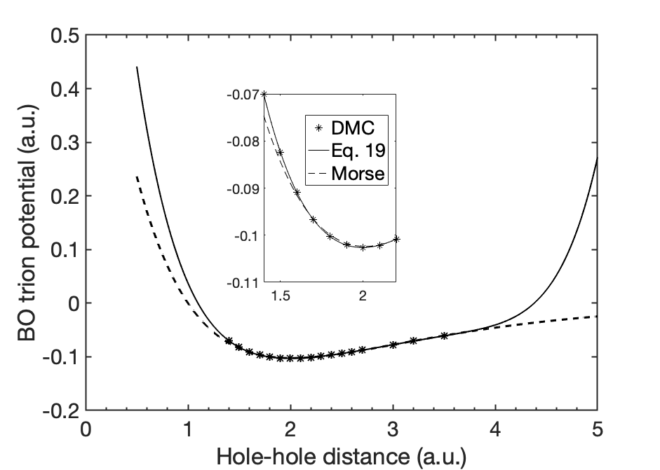
Figure 14: Fits of a Morse potential [Eq. (30), raw DMC data offset by $E_{\text{X}}$] and Eq. (18) to the DMC BO potential of a positive trion. The Morse fitting parameters are $D_{\text{eq}}=0.102553(8)$ a.u., $R_{\text{eq}}=2.0181(1)$ a.u., and $a=0.7003(2)$ a.u. The SSE and RMSE are $6.451\times 10^{-6}$ a.u. and $0.0006788$ a.u., respectively. The value of $R_{\text{eq}}$ is slightly larger than the value predicted by fitting Eq. (18). However, the Morse potential shows much more reasonable behavior at small and large hole-hole separations. The fitted function given by Eq. (18) increases unphysically at large separations beyond $2.6$ a.u. However, Eq. (18) fits the DMC data very well in the vicinity of the equilibrium point, as seen in the inset; consequently spectroscopic constants predicted by Eq. (18), shown in Table 5, are more accurate than those predicted by the Morse potential, shown in Table 19.

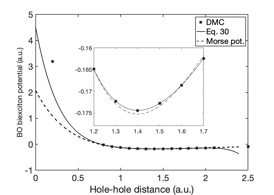
Figure 15: Fits of a Morse potential [Eq. (30), raw DMC data offset by $2E_{\text{X}}$] and Eq. (29) to the DMC BO potential of a biexciton. To obtain a better SSE and RMSE using the Morse model, we only included separations in the range 1 a.u.${}\leq r_{\text{hh}}\leq{}$1.8 a.u. in the fit. The Morse fitting parameters are $D_{\text{eq}}=0.17459(1)$ a.u., $R_{\text{eq}}=1.4054(1)$ a.u., and $a=1.0402(6)$ a.u. The SSE and RMSE are $1.018\times 10^{-5}$ a.u. and RMSE${}=0.001128$ a.u., respectively. The $R_{\text{eq}}$ is close to the value obtained by fitting Eq. (29). In the large separation limit, contrary to the Morse model, Eq. (29) becomes unphysical. In the vicinity of the equilibrium point, Eq. (29) fits the DMC data better and produces more accurate spectroscopic constants, as seen by comparing Tables 10 and 20.

Table 19: Spectroscopic constants obtained from the Morse potential fitted to the DMC BO potential of the positive trion. The fitted parameters are listed in the caption of Fig. 14.

Cation	$\omega_{\text{e}}$ (cm-1)	$\omega_{\text{e}}x_{\text{e}}$ (cm-1)	$\alpha_{\text{e}}$ (cm-1)	$B_{\text{e}}$ (cm-1)
H${}_{2}^{+}$	$2297.4(8)$	$58.63(4)$	$0.9298(7)$	$29.348(4)$
D${}_{2}^{+}$	$1624.9(6)$	$29.33(2)$	$0.3290(3)$	$14.681(2)$
T${}_{2}^{+}$	$1327.8(5)$	$19.58(1)$	$0.1795(1)$	$9.803(1)$

Table 20: Spectroscopic constants obtained from the Morse potential fitted to the DMC BO potential of a biexciton. The fitted parameters are listed in the caption of Fig. 15.

Molecule	$\omega_{\text{e}}$ (cm-1)	$\omega_{\text{e}}x_{\text{e}}$ (cm-1)	$\alpha_{\text{e}}$ (cm-1)	$B_{\text{e}}$ (cm-1)
H2	$4453(3)$	$129.3(1)$	$2.280(3)$	$60.51(1)$
D2	$3149(2)$	$64.70(7)$	$0.807(1)$	$30.271(5)$
T2	$2573(1)$	$43.20(5)$	$0.4401(5)$	$20.213(4)$