Hierarchical Interdisciplinary Topic Detection Model for Research Proposal Classification

Abstract

The peer merit review of research proposals has been the major mechanism to decide grant awards. However, research proposals have become increasingly interdisciplinary. It has been a longstanding challenge to assign interdisciplinary proposals to appropriate reviewers so proposals are fairly evaluated. One of the critical steps in reviewer assignment is to generate accurate interdisciplinary topic labels for proposal-reviewer matching. Existing systems mainly collect topic labels manually generated by principle investigators. However, such human-reported labels can be non-accurate, incomplete, labor intensive, and time costly. What role can AI play in developing a fair and precise proposal reviewer assignment system? In this study, we collaborate with the National Science Foundation of China to address the task of automated interdisciplinary topic path detection. For this purpose, we develop a deep Hierarchical Interdisciplinary Research Proposal Classification Network (HIRPCN). Specifically, we first propose a hierarchical transformer to extract the textual semantic information of proposals. We then design an interdisciplinary graph and leverage GNNs to learn representations of each discipline in order to extract interdisciplinary knowledge. After extracting the semantic and interdisciplinary knowledge, we design a level-wise prediction component to fuse the two types of knowledge representations and detect interdisciplinary topic paths for each proposal. We conduct extensive experiments and expert evaluations on three real-world datasets to demonstrate the effectiveness of our proposed model.

1 Introduction

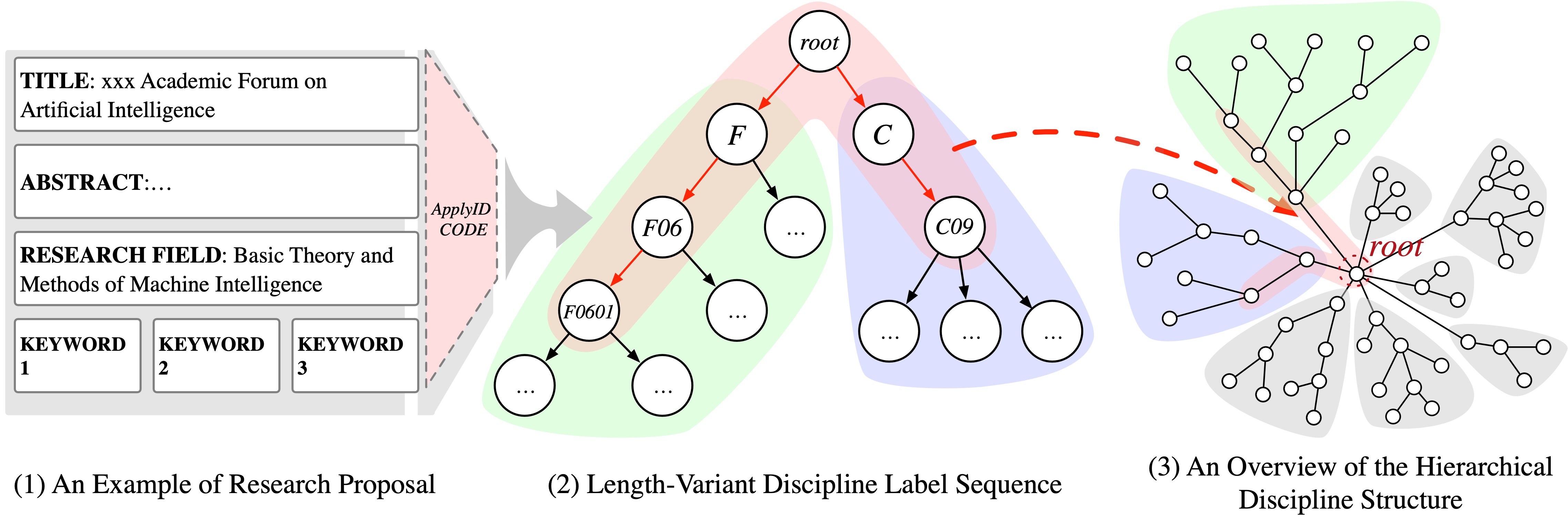
Figure 1: A toy model of the Interdisciplinary Research Proposal Classification.

Nowadays, research funding is awarded based on the intellectual merits and broader impacts of proposals. Under this mechanism, investigators submit research proposals to open-court competitive programs managed by federal agencies (e.g., NSF, NIH). Proposals are then assigned to appropriate reviewers to solicit review comments and ratings. The biggest challenge of running such a peer-review system is to label precise interdisciplinary topics of proposals and allocate appropriate domain experts to obtain effective review comments. However, with the increasing number of universities, faculty members, hired graduate students, and publications, the submissions of research proposals have been exploding [1, 2]. For example, the National Natural Science Foundation of China (NSFC) organizes review panels for more than one million research proposals every year. Due to this growth momentum, there is an urgent need to introduce AI to automated and intelligent proposal labeling for review assignment.

In addition, research proposals increasingly exhibit interdisciplinary characteristics. It is inappropriate to select reviewers from only one field. It, therefore, is highly needed to classify a proposal into one or more disciplines, which we call the task of Interdisciplinary Research Proposal Classification (IRPC). Figure 1 demonstrates an example of the IRPC task. After analyzing large-scale proposals from NSFC, we identify three unique data characteristics. These properties provide great potential to overcome the challenges in the IRPC task:

(Property 1: Hierarchical Discipline Structure) Before embarking on the specific problem, it is worth understanding how the funding administrator regiment the disciplines. In NSFC, thousands of disciplines and sub-disciplines are organized into a hierarchical structure to better index, search, and match reviewers and proposals. Each discipline is associated with a unique alphabetical identifier, which is called ApplyID. An ApplyID is a sequence of alphabetical letters. The ApplyID starts with a capital letter from A to H, representing eight major disciplines (e.g., Mathematical Sciences is marked by the letter A). The capital letter is followed by a sequence of numbers, in which every two numbers stand for a sub-discipline division. Figure 1.2 shows an example disciplinary path: F0601. F represents Information Sciences. 06 represents Artificial Intelligence that is a sub-discipline of Information Sciences. 01 represents Fundamentals of Artificial Intelligence that is a sub-discipline of artificial intelligence.

(Property 2: Interdisciplinarity) Interdisciplinary research is an indispensable part of advancing scientific progress [3]. In NSFC, an interdisciplinary research proposal will be marked by two ApplyID codes and assigned to the reviewers according to those codes. Figure 1.2 shows the ApplyID for an interdisciplinary proposal. This proposal is related to Fundamentals of Artificial Intelligence from the major discipline Information Sciences (F0601) and Neuroscience and Psychology (C09) from the major discipline Life Sciences. A proposal with incorrect or incomplete ApplyID codes will be assigned to wrong or non-expert reviewers, which lead to biased evaluations. Thus, to avoid the destruction of valuable pioneering and interdisciplinary research, it is critical to identify an accurate multiple disciplines for interdisciplinary proposals.

(Property 3: Multiple-type Text) The research proposal consists of multi-type textual data, including abstract, keywords, and title. Different types of text have distinct impacts on the topic path detection process. For example, an expert can identify the coarse-grained discipline (e.g., Information Sciences) of a proposal by reading the title. However, when the expert tries to identify a fine-grained disciplinary category (e.g., the Machine Learning, a sub-discipline of information sciences), they might need to consider the contents of each type (e.g., the introduction). In addition, since texts in most research proposals vary widely in length and structure, stitching each text together results in a severe loss of information.

To model the three unique proprieties, we propose three unique strategies for the IRPC task. First, we adopt the top-down Hierarchical Multi-label Classification (HMC) schema to utilize the hierarchical structure among the disciplines. This schema organize the prediction process level-wisely, thus reducing the candidate target number. Further, a level-wise prediction can generate the topic path under a given partial label, which is practical for a real-world application (e.g., the funding administrators or applicants might provide an unrefined topic path, and the model can generate the rest). Second, the interdisciplinarity among the disciplines can be represented as a weighted graph. We construct an Interdisciplinary Graph and use its topology structure to learn the label (discipline) embedding, thus incorporating the knowledge into each prediction step. Third, we model the semantic information within multiple-type text separately by a hierarchical Transformer architecture. In our design, each type of text will attach with a type token to preserve its type-specific semantic information. The self-attention mechanism in Transformer will also enhance the model’s ability to handle the texts with variate lengths. Based on the above technical insights, we propose Hierarchical Interdisciplinary Research Proposal Classification Network (HIRPCN), a deep learning model with a hierarchical multi-label classification scheme.

In conclusion, our contributions are as follows:

• We identify the critical problems of assigning proposals to its related areas for review. We solve these problems via detecting topic paths on the hierarchical discipline structure.

• We propose HIRPCN, a framework integrating proposals’ semantic information and interdisciplinary topology knowledge for hierarchical label generation, which can generate one or more topic paths for non-interdisciplinary or interdisciplinary proposals.

• The experiments and experts’ evaluations show that our model can generate high-quality prediction results and reveal the candidate interdisciplines for research with incomplete labels.

• We post a demo of our model to demonstrate the process of the topic path detection and how it would aid the funding administrator. Our approach will apply to funding management in the future and contribute to improving the effectiveness and fairness of the science ecosystem.

2 Definitions and Problem Statement

2.1 Important Definitions

2.1.1 A Research Proposal

Applicants write proposals to apply for grants. Figure 1.1 shows a proposal which includes multiple documents such as Title, Abstract, and Keywords, Research Fields, etc. Let’s denote a proposal by $A$, the documents in a proposal are denoted by $D=\{d_{t}\}_{t=1}^{|T|}$ and the types of each document are denoted by $T=\{t_{i}\}_{i=1}^{|T|}$. The $|T|$ is the total number of the document types, and $d_{i}$ is the document of $i$-th type $t_{i}$. Every document $d_{i}$ in the proposal, denoted as $d_{i}=[w^{1}_{i},w^{2}_{i},...,w_{i}^{|d_{i}|}]$, is a sequence of words, where $w^{k}_{i}$ is the $k$-th word in the document $d_{i}$.

2.1.2 Hierarchical Discipline Structure

A hierarchical discipline structure, denoted by $\gamma$, is a DAG or a tree that is composed of discipline entities and the directed Belong-to relation from a discipline to its sub-disciplines. The discipline nodes set $\mathbf{C}=\{C_{0}\cup C_{1}\cup...\cup C_{H}\}$ are organized in $H$ hierarchical levels, where $H$ is the depth of hierarchical level, $C_{k}=\{c^{i}_{k}\}^{|C_{k}|}_{i=1}$ is the set of the disciplines in the $i$-th level. The $C_{0}=\{root\}$ is the root level of $\gamma$. To describe the connection between different disciplines, we introduce $\prec$, a partial order representing the Belong-to relationship. $\prec$ is asymmetric, anti-reflexive and transitive[4]:

$$\bullet\text{The only one greatest category }\textit{root}\text{ is the root of the }\gamma,$$

$$\bullet\forall c^{x}_{i}\in C_{i},c^{y}_{j}\in C_{j},c^{x}_{i}\prec c^{y}_{j}\to c^{y}_{j}\not\prec c^{x}_{i},$$

$$\bullet\forall c^{x}_{i}\in C_{i},c^{x}_{i}\not\prec c^{x}_{i},$$

$$\bullet\forall c^{x}_{i}\in C_{i},c^{y}_{j}\in C_{j},c^{z}_{k}\in C_{k},c^{x}_{i}\prec c^{y}_{j}\land c^{y}_{j}\prec c^{z}_{k}\to c^{x}_{i}\prec c^{z}_{k}.$$

Finally, we define the Hierarchical Discipline Structure $\gamma$ as a partial order set $\gamma=(\mathbf{C},\prec)$.

2.1.3 Topic Path

In this paper, we define the target labels of each research proposal as the Topic Path $\mathbb{L}=[L_{0},L_{1},L_{2},...,L_{H_{A}}]$. $L_{i}=\{l_{i}^{j}\}_{j=1}^{|L_{i}|}$ is a set of the labels in the label paths on the $i$-th level (i.e., $\forall l_{i}^{j}\in L_{i}\to l_{i}^{j}\in C_{i}$). $H_{A}$ is the proper length of label paths. For example, in the Figure 1, the input research proposal are labeled by the ApplyID codes $F0601$ and $C09$. So the $\mathbb{L}$ for this research proposal can be processed as $[\{l_{root}\},\{F,C\},\{F06,C09\},\{F0601,l_{stop}\}]$. The $l_{root}$ stands for the root node of the discipline structure. The $l_{stop}$ is an end-of-prediction token, which is appended to the last set in $\mathbb{L}$ to denote the topic path ended.

2.1.4 Interdisciplinary Graph

A discipline is a combination of domain knowledge and topics. On the one hand, those topics will be carefully selected [5] by the applicants to represent the key idea of their research proposal. On the other hand, the overlapping topic (co-topic) between disciplines could represent their similarity. So, how to measure interdisciplinarity? S. W. Aboelela [6] believes that interdisciplinary research is engaging from two seemingly unrelated fields, which means: (1) these disciplines will have few overlapped topics. (2) those overlapped topics will be frequently cited by the researchers. In this paper, we adopt the Rao-Stirling [7] (RS) to measure interdisciplinarity. The RS is a non-parametric quantitative heuristic, which is widely adopted to measure the diversity in science [7, 8, 9], the ecosystem [10] and energy security [11]. The RS is defined as:

$$RS=\sum_{ab(a\not=b)}(p_{a}\cdot p_{b})^{\alpha}\cdot(d_{ab})^{\beta},$$ (1)

where the first part $\left[\sum_{ab(a\not=b)}(p_{a}\cdot p_{b})\right]$ are proportional representations of elements $a$ and $b$ in the system, and the rest $\left[\sum_{ab(a\not=b)}d_{a,b}\right]$ is the degree of difference attributed to elements $a$ and $b$. The $\alpha$ and $\beta$ are two constant to weighting the two components. We introduce the RS in a micro view to define the weight on $e_{a\to b}$:

$$e_{a\to b}=(p_{a\to b})^{\alpha}(d_{a\to b})^{\beta},$$ (2)

where $p_{a\to b}$ is the proportion of the proposals in discipline $a$ that contain same topics in $b$, which represents the co-selected frequency of $a$ to $b$. $d_{a\to b}$ is the proportion of topic overlap from $a$ to $b$. Their detailed definitions are as:

$$p_{a\to b}=\frac{\sum_{i}^{n}\mathbbm{1}(k_{i}\in\{K_{a}\cap K_{b}\})F_{a}[k_{i}]}{\sum_{i}^{n}F_{a}[k_{i}]},$$ (3)

$$d_{a\to b}=1-\frac{|K_{a}\cap K_{b}|}{|K_{a}|},$$ (4)

where the $\mathbbm{1}(\cdot)\to\{0,1\}$ is the indicator function, $K_{a}$ and $K_{b}$ are topic set of $a$ and $b$, $n$ is the total number of the topic. $F_{a}$ and $F_{b}$ are two lookup table holding the frequency of each topic being selected in the proposals that relat to $a$ and $b$.

By that, we build a Interdisciplinary Graph, denoted as $G=(\mathbf{C},E)$, to represent the interdisciplinarity among disciplines. $G$ is a collection of discipline set $\mathbf{C}$ and directed weighted edge set $E=\left\{e_{a\to b}\right\}^{|\mathbf{C}|}_{a,b=1}$. Each $e_{a\to b}\geq 0$ represents the interdisciplinary strength from discipline $a$ to discipline $b$.

2.2 Problem Formulation

We formulate the IRPC task in a hierarchical classification schema and use a sequence of discipline-level-specific label sets $\mathbb{L}$ as topic path to represent the proposals’ disciplinary codes. To sum up, given the proposal’s document set $D$ and the interdisciplinary graph $G$, we decompose the prediction process into an top-down fashion from the beginning level to the certain level on the hierarchical discipline structure $\gamma$. Suppose the $k-1$ ancestors labels in $\mathbb{L}$ are $\mathbb{L}_{<k}=[L_{0},L_{1},...,L_{k-1}]$, where $\mathbb{L}_{<1}=\{L_{0}\}$. The prediction on level $k$ can be seen as a multi-label classification task on $C_{k}$ based on the incomplete topic path $\mathbb{L}_{<k}$, this process can be defined as:

$$\Omega(D,G,\gamma,\mathbb{L}_{<k};\Theta)\to L_{k},$$

where $\Theta$ are the parameters of model $\Omega$. Also, we use the end-of-prediction label $l_{stop}$ in the last set $L_{H_{A}}$ to mark the proper level (i.e., the $H_{A}$) where the model to stop on. Eventually, we can formulate the probability of the topic path assignment as:

$$P(\mathbb{L}|D,G,\gamma;\Theta)=\prod_{k=1}^{H_{A}}P(L_{k}|D,G,\gamma,\mathbb{L}_{<k};\Theta)$$ (5)

where $P(\mathbb{L}|D,G,\gamma;\Theta)$ is the overall probability of the proposal $A$ belonging to the label set sequence $\mathbb{L}$, $P(L_{k}|D,G,\gamma,\mathbb{L}_{<k};\Theta)$ is the label set assignment probability of $A$ in level-$k$ when given the previous ancestor $\mathbb{L}_{<k}$. In training, given all the ground truth labels, our goal is to maximize the Equation 5.

3 Interdisciplinary Topic Detection

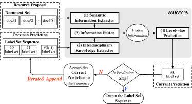
Figure 2: An overview figure of the HIRPCN during the level-$k$ prediction.

3.1 Overview of the Proposed Framework

Figure 2 illustrate iteration of our framework upon four components: (1) Semantic Information Extractor (SIE) models the semantic components in research proposals according to their particular type (e.g., title, abstract, keywords, research fields) and encodes them into a matrix. (2) Interdisciplinary Knowledge Extractor (IKE) obtains the representation of previous prediction results from the pre-built interdisciplinary graphs. (3) Information Fusion (IF) fuses the type-specific semantic information and the representation of previous prediction results. (4) Level-wise Prediction (LP) predicts the probability that a research proposal falls within particular disciplines at the current step. After completing this iteration, our framework takes the discipline predictions, appends them to the label set sequence, and then moves to the next step. The initial input of the model will be the root node in the hierarchical discipline structure and a document set from a research proposal. The model will incrementally complete the input research proposal’s label path as the iteration goes on until the end-of-prediction label has been generated.

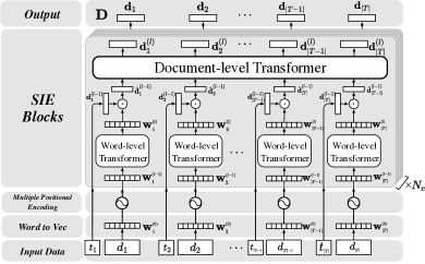
Figure 3: Illustration of Semantic Information Extractor. The $\odot$ means integrating operation between vanilla document representation and their type information.

3.2 Semantic Information Extractor

Figure 3 shows the overview of SIE. SIE comprises a Word to Vec layer, a Multiple Positional Encoding (MPE) layer, and multi-layer SIEBlocks. Each SIEBlock consists of two parts: a word-level Transformer and a document-level Transformer. Formally, the representation of a proposal is obtained by:

$$\mathbf{D}=N_{e}\times SIEBlock(\{\mathbf{W}_{i}^{(0)}\}_{i=1}^{|T|}),$$ (6)

where the matrix $\mathbf{D}$ is the representation of the input research proposal. $\mathbf{W}_{i}^{(0)}$ is the word embedding matrix of the document $d_{i}$. The $N_{e}$ is the total layer number of SIEBlocks.

Our Perspective: We consider two essential aspects of the research proposal. First, different types of documents (e.g., title, abstract, keywords, research fields) in a research proposal should be separately weighed when identifying the topic path of the proposal. Second, in the proposal, each document varies in length (e.g., title and abstract), and concatenating them together will cause a severe loss of information. Inspired by the long-text modeling methods [13, 14, 15], we design a hierarchical Transformer architecture to embed both texts and their particular type within a proposal into a matrix.

Step 1: Word to Vec and Multilple Positional Encoding. We first vectorize each words in document by a pre-trained $h$-dimensional Word2Vec [16] model, then sum them with positional encoding to preserve the position information. After separately concatenating each document’s word vector, we can obtain the word embedding. It is worth noting that we padded each document to an identical length before the Word to Vec component. The length of each document after padding is denoted by $|d|$. The word embedding for document $d_{i}$ is denoted as $\mathbf{W}^{(0)}_{i}\in\mathbb{R}^{|d|\times h}$. Then we seperately feed each document representation matrix into the multi-layer SIEBlocks.

Step 2: Word-level Transformer. In the first stage of $l$-th SIEBlock, we aim to use a word-level Transformer to extract the contextual semantic information. We can obtain the document representation matrix $\mathbf{W}^{(l-1)}_{i}\in\mathbb{R}^{|d|\times h}$ from the previous layer. Then, we can formulate the process of the current layer as:

$$\mathbf{W}^{(l)}_{i} =Transformer_{w}(\mathbf{W}^{(l-1)}_{i}),$$ (7)

where the $\mathbf{W}^{(l)}_{i}\in\mathbb{R}^{|d|\times h}$ is the vanilla document representation matrix in current layer. The ${Transformer}_{w}(\cdot)$ is the word-level Transformer block in $l$-th SIEBlock.

Step 3: Document-level Transformer. In the second stage of $l$-th SIEBlock, we aim to fuse each vanilla document representation matrix with its correlated type information by a document-level Transformer:

$$\mathbf{D}^{(l)}={Transformer}_{d}(\{\mathbf{d}^{(l-1)}_{i}\odot\mathbf{W}^{(l)}_{i}\}_{i=1}^{|T|}),$$ (8)

where ${Transformer}_{d}(\cdot)$ is the document-level Transformer block. $\mathbf{d}^{(l-1)}_{i}\in\mathbb{R}^{h}$ is the type-specific representation of $d_{i}$ from previous layer.In the first layer, the model will initialize each document’s type-specific representation with a randomly initialized look-up table according to their type $t$. And the $\odot$ is a fusing operation.

Inspired by ViT[17] and TNT[18], we set the $\odot$ operation as: (1) a Vectorization Operation on $\mathbf{W}^{(l)}_{i}$. (2) a Fully-connected Layer to transform the vanilla document representation from dimension $|d|h$ to dimension $h$. (3) an Element-wise Add with the vector $\mathbf{d}^{(l-1)}_{i}$ from previous layer to obatin the type-specific representation in current layer. $\mathbf{D}^{(l)}\in\mathbb{R}^{|T|\times h}$ is the outputs of current layer, which can be seen as $|T|$-views of high-level abstraction for proposals. After $N_{e}$ times propagation, we can obtain the final output of SIE as $\mathbf{D}=\mathbf{D}^{(N_{e})}$.

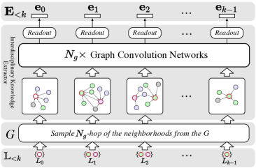
Figure 4: Illustration of Interdisciplinary Knowledge Extractor. The colors of the circles represent their belonging disciplines. We use the red outline to mark the central nodes.

3.3 Interdisciplinary Knowledge Extractor

The IKE is aimed to acquire the embedding of each prediction step from the pre-built interdisciplinary graph $G$. Figure 4 shows an overview of IKE, which consists of multi-layer Graph Covolutional Network (GCN) and a Readout Layer. From an overall perspective, the label embedding is learned by:

$$\mathbf{E}_{<k}=IKE(\mathbb{L}_{<k},G),$$ (9)

where the $\mathbf{E}_{<k}\in\mathbb{R}^{k\times h}$ is the matrix to preserve the prediction state and interdisciplinary knowledge from previous $k-1$ steps.

Our Perspective: Embed the Previous Prediction. We usually model people’s behavior by capturing their relationships with others on the social network graph. The same idea is adopted in IKE to extract the previous prediction state from the interdisciplinary graph. Instead of inputting the former prediction result directly or passing a hidden state between each step, our design uses the previous results and their neighborhood on the interdisciplinary graph to obtain the representation of each step.

Step 1: Obtain the Representation. Suppose we are processing the $k$-th step. Given the sequence of label sets $\mathbb{L}_{<k}=[L_{0},L_{1},...,L_{k-1}]$ from the previous $k-1$ steps (or from a manually given partial label). Each label set $L_{i}$ consists of the disciplines for holding the prediction result in the $i$-th step. We first treat the including discipline nodes as the central node and sample their $N_{g}$-hops neighborhoods (as an adjacency weighted matrix) from the interdisciplinary graph $G$, where the $N_{g}$ is the total layer number of GCN. Then we feed the adjacency weighted matrix and its corresponding node features into the GCN:

$$\mathbf{H}_{i}=N_{g}\times GCN(E_{i},\mathbf{H}^{(0)}_{i}),$$ (10)

where the $\mathbf{H}^{(0)}_{i}$ is a random initialized input feature of the central nodes and their $N_{g}$-hops neighborhood nodes. The $E_{i}$ is the weighted adjacency matrix between these nodes. The $\mathbf{H}_{i}$ is the output matrix undergoing $N_{g}$ times GCN propagations.

Step 2: Readout the Features. Due to the varied number of discipline nodes within each prediction label set, we have to pool the matrix and acquire the representations of each step. For example, the representation of $L_{i}$ is obtained by:

$$\mathbf{e}_{i}=Readout(\mathbf{H}_{i},L_{i}),$$ (11)

where the Readout layer is a lookup operation (i.e., take the $L_{i}$ included node embedding) followed by a mean pooling layer. The $\mathbf{e}_{i}\in\mathbb{R}^{h}$ is the final representation of $L_{i}$. Then we can obtain the output of IKE as $\mathbf{E}_{<k}=[\mathbf{e}_{0},\mathbf{e}_{1},...,\mathbf{e}_{k-1}]$.

The $\mathbf{E}_{<k}$ can be seen as the representation of the prediction results from the previous $k-1$ steps integrated with their neighborhoods information from the interdisciplinary graph. We believe that the neighborhood information could help the model more inclined to predict the discipline that is highly connected to the historical predicted discipline on the interdisciplinary graph, thereby improving the ability to predict the interdisciplinary.

3.4 Information Fusion

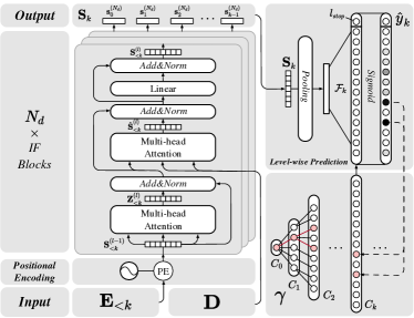
Figure 5: Illustration of Information Fusion and Level-wise Prediction in step-$k$.

In IF, we use a multi-layer IF Block to integrate the extracted information from SIE and IKE. As the left side of Figure 5 shows, the IF consists of a positional encoding and multi-layer IFBlocks. We start the introduction by giving its dataflow:

$$\mathbf{S}_{k}=N_{d}\times IFBlock(\mathbf{E}_{<k},\mathbf{D}),$$ (12)

where $N_{d}$ is the total layer number of IF Block, and $\mathbf{S}_{k}\in\mathbb{R}^{k\times h}$ is the fusion matrix that integrated the semantic information and the previous prediction information with interdisciplinary knowledge.

Our Perspective: Adaptively Utilize Each Part of Information. There are two aspects we consider in IF. First, the current prediction state should be significantly affected by its previous results. Second, the model should adaptively choose the critical part of semantic information according to its current prediction state. To advance those, we divide the IF into two steps.

Step 1: Positional Encoding and Previous Label Embedding Fusion. We first sum the $\mathbf{E}_{<k}$ with positional encoding to obtain $\mathbf{S}_{<k}^{(0)}$ for preserving the order of prediction. Then, in layer-$(l)$ we perform Multi-Head Self-Attention between each prediction result representation to help each element in $\mathbf{S}_{<k}^{(l-1)}$ aggregate knowledge from their context:

$$\hat{\mathbf{S}}^{(l)}_{<k}=\mathbf{S}_{<k}^{(l-1)}\circ\textit{MultiHead}(\mathbf{S}_{<k}^{(l-1)},\mathbf{S}_{<k}^{(l-1)},\mathbf{S}_{<k}^{(l-1)})),$$ (13)

where $\circ$ operation is a Layer Normalization with a Residual Connection Layer. In this step, the $\textit{MultiHead}(\cdot)$ adaptively aggregate the context information from every step prediction, and the $\circ$ operation integrate the context knowledge to the prediction result embedding and form the the level-$l$ prediction state as $\hat{\mathbf{S}}^{(l)}_{<k}\in\mathbb{R}^{k\times h}$. With the order information, we believe step 1 of IF can capture the hierarchical dependency and the interdisciplinary knowledge in $\mathbb{L}_{<k}$

Step 2: Obtain the Semantic Informaion Adaptively. As mentioned before, we hope our model can utilize each part of the research proposal adaptively through prediction progress. Thus, we treat the prediction state $\hat{\mathbf{S}}^{(l)}_{<k}$ as Query and the representation of document set $\mathbf{D}$ as Key and Value into another Multi-head Attention to propagate the semantic information:

$$\mathbf{Z}^{(l)} =\hat{\mathbf{S}}^{(l)}_{<k}\circ\textit{MultiHead}(\hat{\mathbf{S}}^{(l)}_{<k},\mathbf{D},\mathbf{D})),$$ (14)

$$\mathbf{S}_{<k}^{(l)} =\mathbf{Z}^{(l)}\circ FC(\mathbf{Z}^{(l)}),$$

The $\textit{MultiHead}(\cdot)$ adaptively aggregate the semantic information from the research proposal by the current prediction state, and the $\circ$ operation integrate the semantic information to the label embedding and construct the hidden feature $\mathbf{Z}^{(l)}\in\mathbb{R}^{k\times h}$ in level-$l$. After a Fully-connected Layer denoted as $FC(\cdot)$ and the $\circ$ operation, we form $\mathbf{S}_{<k}^{(l)}$ to hold the fusion information in level-$l$.

After $N_{d}$ times propagations, we acquire the $\mathbf{S}_{k}=\mathbf{S}_{<k}^{(N_{d})}$ to represent the output of IF. With the IF, the model will learn the dependency between previous prediction steps and adaptively fuse each part of semantic information by the current prediction progress.

3.5 Level-wise Prediction

The right side of Figure 5 demonstrate the prediction in step-$k$. In LP, We feed the fusion feature matrix $\mathbf{S}_{k}$ into a Pooling Layer, a Fully-connected Layer, and a Sigmoid Layer to generate each label’s probability for $k$-th level-wise label prediction.

$$y_{k}=Sigmoid(FC_{k}(Pooling(\mathbf{S}_{k}))),$$ (15)

where the $y_{k}$ is the probability (i.e., $P(L_{k}|D,G,\gamma,\mathbb{L}_{<k};\Theta)$ in Equation 5) for each discipline in $k$-th level of hierarchical discipline structure $\gamma$. It is worth noting that we add a $l_{stop}$ token in each step to determine the prediction state. Thus, the $FC_{k}(\cdot)$ denotes a level-specific feed-forward network with a ReLU activation function to project the input to a $|C_{k}|+1$ length vector, where represents the label number of level-$k$ with $l_{stop}$ token. After the $Sigmoid(\cdot)$, the final output $y_{k}$ is the probability of $k$-th level’s labels. Thus, the level-$k$’s objective function $\mathcal{L}_{k}$ can be defined as:

$$\mathcal{L}_{k}(\Theta) =\sum^{\mid C_{k}\mid+1}_{i=1}\left(Y_{k}(i)\log(y^{i}_{k})+(1-Y_{k}(i))\log(1-y^{i}_{k})\right),$$ (16)

$$\text{where }Y_{k}(i)=\begin{cases}0:l_{i}\not\in L_{k}\\ 1:l_{i}\in L_{k}\end{cases},$$

where the $y^{i}_{k}$ is the probability of the level-$k$’s $i$-th label.

The label prediction starts from the 1st level with given $\mathbb{L}_{<1}$. In the $k$-th level prediction, the label corresponding to the index of the value in the $y_{k}$ which achieves the threshold will be selected to construct the current prediction result set $L_{k}$. The model will append the $L_{k}$ to $\mathbb{L}_{<k}$ to construct $\mathbb{L}_{k}$ as current prediction result. If the prediction continues, $\mathbb{L}_{k}$ will form the next previous prediction result $\mathbb{L}_{<(k+1)}$. To require that the model can define a distribution over labels of all possible lengths, we add a end-of-prediction label $l_{stop}$ token and set the first element of $y_{k}$ as the probability of $l_{stop}$ in level-k. In the final step, the $l_{stop}$ will include in the prediction target.

We sum the loss in each level to obtain the overall loss function of HIRPCN as:

$$\mathcal{L}(\Theta)=\sum\mathcal{L}_{k}(\Theta).\\$$ (17)

During the training process, our target is to optimize the objective function $\mathcal{L}(\Theta)$.

3.6 Application

Our proposed method (HIRPCN) aims to generate the topic path for an input research proposal. In real world scenario, the applicants will submit the research proposals and the ApplyID codes. Then the fund administrator will assign reviewers depending on the given ApplyID codes. This framework can introduce AI as an assistant to address: 1) the barrier between the applicant and the complex discipline structure; 2) the missed or concealed topic information. Besides these, the design of IKE can let the model start prediction from any given level, making the applicants only need to provide coarse-grained labels, which is essential for online guidance. Lastly, the attention mechanism can provide interpretability for model prediction, and its visualization can facilitate the fund administrator to verify each research proposal’s topic path.

4 Experiments

In this section, we conducted experiments to evaluate the performance of HIRPCN and answer the following questions: Q1. Is the performance of HIRPCN superior to the existing baseline models? Q2. How is each component of HIRPCN affect the performance? Q3. Can HIRPCN achieve the best performance on the prediction at all levels? Q4. How good is the prediction result? Q5. Can the given partial expert advice improve the performance of HIRPCN? Q6. Can HIRPCN adaptively utilize the semantic information and historical prediction results? Q7. How is the word-level attention mechanism works for a better semantic extraction? Q8. What is the extra generated label significance to the peer-review assignment? We also evaluated the model performance from different settings of interdisciplinary graphs and hyperparameters.

4.1 Experimental Setup

4.1.1 Dataset Description

We collected research proposals written by the scientists from 2020’s NSFC research funding application platform, containing 280683 records with 2494 ApplyID codes. As shown in Table  I, when the level goes deeper, since there is more number of disciplines, the classification becomes harder. In data processing, we chose four parts of a research proposal as the document data: 1) Title, 2) Keywords, 3) Abstract, 4) Research Field. The Abstract part is in long-text form, and the average length is 100. The rest three documents are all short text. We removed all the punctuation and padded the length of each document to 200. Then we added a type-token at the beginning of each document to mark its particular type (just like the [CLS] token in the Bert[21]). For the label construction, we generate the topic path of each research proposal (as described in Section 2.1.3). We further organized and divided those processed data by their interdisciplinarity into three datasets:

• RP-all: An overall dataset with all kinds of research proposals, whether interdisciplinary research or non-interdisciplinary research.

• RP-bi: Including all research proposals with two major disciplines or one major discipline but gets interdisciplinarity in its sub-discipline.

• RP-differ: Only includes the interdisciplinary research proposals with two major disciplines and its data shows the most interdisciplinarity among the three datasets.

In Table II, we counted the lengths of each label sequence and the average number of level-wise labels on three datasets. Generally speaking, from RP-all to RP-differ, the data exhibit interdisciplinarity increasingly and becomes more challenging to detect its topic path. The comparison of model performance between these datasets can evaluate the specific design of HIRPCN.

TABLE I: The discipline and sub-discipline numbers on each level of hierarchical discipline structure.

Prefix	Major Discipline Name	Total	$|C_{2}|$	$|C_{3}|$	$|C_{4}|$
A	Mathematical Sciences	318	6	57	255
B	Chemical Sciences	392	8	59	325
C	Life Sciences	801	21	162	618
D	Earth Sciences	166	7	94	65
E	Engineering and Materials Sciences	138	13	118	7
F	Information Sciences	100	7	88	5
G	Management Sciences	107	4	57	46
H	Medicine Sciences	456	29	427	0
-	Total Disciplines	2478	95	1062	1321

TABLE II: The Details of Three Datasets.

Dataset	RP-all	RP-bi	RP-differ
Total Proposal Number	280683	125466	20632
#Avg. Labels Length	2.393	3.355	3.397
#Avg. Labels Num in Level-1	1.073	1.164	2.000
#Avg. Labels Num in Level-2	1.197	1.442	2.000
#Avg. Labels Num in Level-3	1.364	1.870	1.985
#Avg. Labels Num in Level-4	0.477	0.726	0.808

4.1.2 Baseline Algorithms

We compared our model with seven Text Classification (TC) methods including TextCNN [22], DPCNN [23], FastText [24, 25], TextRNN [26], TextRNN-Attn [27], TextRCNN [28], Trasnformer [12] and three state-of-the-art HMC approaches including HMCN-F, HMCN-R [29], and HARNN [30]. We choosed three Hierarchical Multi-label Text Classification (HMTC) methods including HE-AGCRCNN[31], HiLAP[32], two variants of HiAGM[33] (i.e., HiAGM-LA and HiAGM-TP). We also posted three ablation models of HIRPCN as baselines, including w/o Interdisciplinary Graph (w/o IKE), w/o Hierarchical Transformers (w/o SIE), and w/o ALL. We summarized four critical attributes of these baseline models in Table III as:

• Hierarchical Awareness: represents whether the model uses the hierarchical information of the label structure to enhance the model performance.

• Text-type Awareness: represents whether the model is aware of the document type within each part of the research proposal.

• Interdisciplinary Awareness: represents whether the model can utilize the interdisciplinary knowledge in the discipline system, i.e., the interdisciplinary graph.

• Start Prediction From Anywhere: represents whether the model can start prediction with a given partial label, which is critical when aiding applicants and administrators in judging the proposal belongings.

4.1.3 Evaluation Metrics

To fairly evaluate the HIRPCN with other baselines, we adopted several metrics from the Multi-label Classification [34, 35, 36], i.e., the Micro-F1 (MiF1), and Macro-F1 (MaF1). We conducted a 5-fold cross-validation and reported the average recommendation performance.

4.1.4 Hyperparameters, Source Code and Reproducibility

We set the SIE layer number $N_{e}$ to 8, the dimension size $h$ to 64, and the multi-head number to 8. The IKE layer number $N_{g}$ is set to 1. The IF layer number $N_{d}$ is set to 8, and the multi-head number is set to 8. We pre-trained the word embedding with a dimension ($h$) 64 via Word2Vec[16] model. For the detail of training, we use Adam optimizer[37] with a learning rate of $1\times 10^{-3}$, and set the mini-batch as 512, adam weight decay as $1\times 10^{-7}$. The dropout rate is set to $0.2$ to prevent overfitting. The warm-up step is set as 1000. The $\alpha$ and $\beta$ for interdisciplinary graph construction set to 0.1. We shared the source code via Dropbox.

4.1.5 Environmental Settings

All methods are implemented by PyTorch 1.8.1[38]. The experiments are conducted on a CentOS 7.1 server with a AMD EPYC 7742 CPU and 8 NVIDIA A100 GPUs.

4.2 Experimental Results

TABLE III: Experimental results on all dataset. The best results are highlighted in bold. The second-best results are highlighted in underline.

Dataset					RP-all		RP-bi		RP-differ
Attributes	Hierarchical Awareness	Text-type Awareness	Interdisciplinary Awareness	Start Prediction From Anywhere	MiF1	MaF1	MiF1	MaF1	MiF1	MaF1
TextCNN	✗	✗	✗	✗	0.456	0.168	0.426	0.148	0.438	0.063
DPCNN	✗	✗	✗	✗	0.376	0.108	0.364	0.080	0.346	0.020
FastText	✗	✗	✗	✗	0.460	0.167	0.427	0.149	0.432	0.067
TextRNN	✗	✗	✗	✗	0.402	0.100	0.364	0.077	0.351	0.021
TextRNN-Attn	✗	✗	✗	✗	0.413	0.098	0.367	0.072	0.338	0.018
TextRCNN	✗	✗	✗	✗	0.426	0.138	0.381	0.100	0.367	0.025
Transformer	✗	✗	✗	✗	0.370	0.083	0.339	0.066	0.358	0.023
HMCN-F	✓	✗	✗	✗	0.676	0.459	0.582	0.308	0.569	$\underline{0.161}$
HMCN-R	✓	✗	✗	✗	0.599	0.289	0.506	0.185	0.478	0.069
HARNN	✓	✗	✗	✗	0.686	0.443	0.574	0.294	0.516	0.102
HE-AGCRCNN	✓	✗	✗	✗	0.513	0.331	0.467	0.289	0.463	0.118
HiLAP	✓	✗	✗	✗	0.628	0.418	0.536	0.280	0.528	0.141
HiAGM-LA	✓	✗	✗	✗	0.594	0.400	0.505	0.258	0.501	0.134
HiAGM-TP	✓	✗	✗	✗	0.629	0.428	0.548	0.285	0.535	0.135
w/o ALL	✓	✗	✗	✓	0.704	0.429	0.583	0.259	0.512	0.098
w/o SIE	✓	✗	✓	✓	0.710	0.438	0.587	0.276	0.533	0.099
w/o IKE	✓	✓	✗	✓	0.737	0.488	0.636	0.329	0.577	0.127
HIRPCN	✓	✓	✓	✓	0.748	0.512	0.648	0.384	0.635	0.180

4.2.1 RQ1: Overall Comparison

We evaluated every method on all datasets and reported the results in Table III. To compare the overall performance of the different models, we organized each step’s prediction results flatly. Then, we used the MiF1 and the MaF1 as the overall evaluation metrics. From the results, we can observe that: Firstly, the HIRPCN achieved the best performance among all datasets, proving that HIRPCN could better solve the challenges mentioned in the IRPC task. Besides this, the methods with top-down HMC schema (e.g., HMCN, HARNN, HIRPCN, and its variants) universally performed better than TC methods. The first reason is that the methods with top-down HMC schema organize the labels in a hierarchical view rather than a flat view, which can reduce the candidate label number in each step. Secondly, one of the critical attributes of the top-down HMC schema is that the model will generate the current prediction base on its previous prediction state. Because there are fewer categories in the earlier levels, the classification in these levels will be easier to predict correctly. Thus, the precise former results will facilitate the performance of these methods in the rest steps. We can also observe that the HMTC methods (e.g., HE-AGCRNN, HiLAP, and HiAGM) performed better than the TC method but slightly worse than the HMC methods. The reason for the former is although their encoder is similar to the TC methods, the HMTC methods either adopted the hierarchical structure into loss function (e.g., the HE-AGCRNN), initialized the label embedding by hierarchical structure (e.g., the HiAGM and its variants), or explicitly using the dependency of each label(e.g., the HiLAP). The latter is because we adopted the Hierarchical Transformer-based encoder for semantic information extraction in these HMC methods, which is more suitable for modeling long text. Further, we noticed that the model’s performance on the three datasets gradually declined. As we mentioned before, the interdisciplinary proposals have more labels on each level, making the classification task harder. The performance on RP-bi is better than that on RP-differ, indicating due to the disparity between the two major disciplines, identifying the topic path under them will become much more challenging. Also, the performance of HIRPCN is better than other baselines, showing its robustness and generalization on the datasets with different interdisciplinarity.

4.2.2 RQ2: Ablation Study

We also discussed the performance of each ablation variant of HIRPCN. The w/o SIE replaced the SIE component with a vanilla Transformer, making the model unable to discriminate the different types of documents (no Text-type Awareness). The w/o IKE removed the IKE component. In each prediction step, w/o IKE will initialize the input previous prediction results by a look-up table (no Interdisciplinary Awareness). The w/o ALL ablated both the IKE and SIE to represent the blank control group. From the Figure III, we can observe that: First of all, the HIRPCN beats all its ablation variants. This observation proves that both SIE and IKE component is valid in our model design. We also noticed that w/o SIE performs worse than w/o IKE in each dataset (e.g., from -3.8% to -8.2% deterioration on Micro-F1). This phenomenon indicates that the type-specific semantic information will play a more critical role in topic path detection. Secondly, w/o IKE performed slightly worse (e.g., -1.5% deterioration on Micro-F1) than HIRPCN on the RP-all dataset, while this deterioration (e.g., -1.9% and -9.1% in Micro-F1) becomes larger on RP-bi and RP-differ. This phenomenon proves that the interdisciplinary knowledge plays a significant role in the classification of interdisciplinary proposals. Lastly, HIRPCN and w/o IKE, both with hierarchical Transformer, are significantly superior to other HMC methods on RP-all and RP-bi, showing the advantage of modeling various lengths of the documents and the multiple types of text for proposal embeddings.

4.2.3 RQ3: Level-wise Performance

TABLE IV: Experimental results on RP-differ in level-wise. The best results are highlighted in bold. The second-best results are highlighted in underline.

Level	1		2		3		4
Metric	MiF1	MaF1	MiF1	MaF1	MiF1	MaF1	MiF1	MaF1
TextCNN	0.735	0.600	0.403	0.285	0.254	0.067	0.190	0.040
DPCNN	0.689	0.543	0.284	0.151	0.132	0.017	0.084	0.009
FastText	0.730	0.610	0.402	0.303	0.251	0.078	0.164	0.037
TextRNN	0.692	0.569	0.296	0.155	0.130	0.018	0.073	0.009
TextRNN-Attn	0.677	0.548	0.278	0.148	0.125	0.015	0.071	0.008
TextRCNN	0.690	0.559	0.310	0.183	0.165	0.025	0.105	0.010
Transformer	0.702	0.577	0.308	0.183	0.135	0.022	0.070	0.009
HMCN-F	0.782	0.670	0.565	0.461	0.460	0.201	0.341	0.102
HMCN-R	0.770	0.664	0.478	0.339	0.278	0.074	0.183	0.041
HARNN	0.793	0.683	0.529	0.409	0.341	0.122	0.226	0.058
HE-AGCRCNN	0.743	0.693	0.439	0.411	0.289	0.132	0.171	0.068
HiLAP	0.732	0.624	0.523	0.418	0.419	0.172	0.306	0.082
HiAGM-LA	0.702	0.610	0.509	0.402	0.398	0.169	0.265	0.069
HiAGM-TP	0.731	0.627	0.538	0.430	0.429	0.178	0.314	0.084
w/o ALL	0.810	0.692	0.564	0.441	0.357	0.133	0.219	0.060
w/o SIE	0.812	0.703	0.551	0.445	0.369	0.138	0.223	0.065
w/o IKE	0.825	0.715	0.627	0.506	0.429	0.150	0.281	0.075
HIRPCN	0.846	0.731	0.658	0.540	0.519	0.222	0.368	0.114

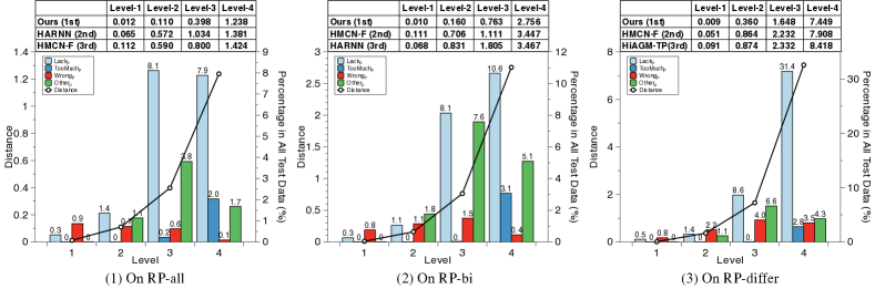
Figure 6: The details of the wrong case and level-wise prediction distance on three datasets. The attached table also reported the interdisciplinary distances of the second and third-best methods.

We reported the performance of level-wise prediction of HIRPCN and other baselines on the RP-differ dataset. Table IV showed the level-wise Micro-F1 and level-wise Macro-F1 classification results on four levels. From the results, we can observe that HIRPCN outperforms all the baseline methods and the variants on every level, showing the advanced ability of the classification at all granularity. We also observed that the performance of each model tends to decrease with the depth of level increase. The reason is that the number of categories increases rapidly, making the classification task harder. We also noticed that Macro-F1 dropped relatively more suddenly than Micro-F1 on each method. From the dataset statistic, we interpreted this as: 1) the length of the label path is variable, so in some cases, the last two levels might contain no target. 2) the test set is imbalanced, so some disciplines might not contain samples. Thus, the Macro-F1 will be lower than Micro-F1, especially in the last two levels. The level-wise model performance on RP-all and RP-bi show the same tendency as on RP-differ so we won’t go into detail.

4.2.4 RQ4: Evaluation of Prediction Results

The Micro-F1 and the Macro-F1 can measure how accurate the prediction is. However, it might be insufficient to evaluate the HIRPCN in real-world applications. In this experiment, we conducted two statistical analyses on three datasets for prediction results. The first analysis evaluates how close the prediction is to the truth label. For instance, if given a truth label in the 3rd level as $\{\textit{A0101}\}$, a prediction $\{\textit{A0102}\}$ might be more acceptable than $\{\textit{B0101}\}$, although they are both wrong. Based on that, we developed a metric named interdisciplinary distance given as:

$$\mathcal{D}(L_{k},\hat{L}_{k})=\sum_{l\in L_{k}}min(\left\{dis(l,\hat{l})\right\}_{\hat{l}\in\hat{L}_{k}}),$$ (18)

where $L_{k}$ and $\hat{L}_{k}$ are the truth labels and the prediction results in level-$k$, respectively. $min(\cdot)$ will take the minimized value from a given set. We adopted a revised edit distance as the distance function $dis(\cdot)$. In detail, if any two-digit or major discipline in the predicted ApplyID code is different from the truth, the function will instantly return the penalty. By discussing it with funding agencies, we set the penalty as $\{1,10,30,50\}$, depending on the remaining step. For example, the distance between A0101 and A0102 will be $1$ due to they are different in level-$3$, and the remaining step will be $0$. And the distance between A0101 and B0101 will be $30$ because they are already different in the first level and their remaining step will be $2$. Also, if $l$ or $\hat{l}$ is null (i.e., the $L_{k}$ or $\hat{L}_{k}$ is empty), the distance will be $k$. Thus, $\mathcal{D}(L_{k},\hat{L}_{k})$ will quantitatively assess the distance between truth label set $L_{k}$ and predicted set $\hat{L}_{k}$. Then, we level-wise average the distance of every sample from the test set. The higher average interdisciplinary distance represents the prediction for this level-$k$ are more offset. Another analysis is we count the appearance number of three wrong cases, i.e., Lack, TooMuch, Wrong, and Other. Lack represents the prediction in the current level is null, which means the model stop at a coarse level. TooMuch means the model step into a too-fine-grained level, and the truth label in the current level is null. Wrong represents that the model gives a prediction that not following the hierarchy. Other represents all other wrong cases.

We calculated the average distance of each level and counted the number of wrong cases. The results of these analyses were reported in Figure 6. Firstly, we can observe that the interdisciplinary distance and the number of wrong cases grow from level-1 to level-4, which is the same as the observation of the decline of Micro-F1 and Macro-F1 in Table III. Secondly, HIRPCN outperforms the second and third-best methods in the distance and shows excellent superiority in the first few levels. This observation shows the same phenomenon as the comparison with Micro-F1 and Macro-F1 in Table III. Furthermore, due to the most happening wrong cases in the level-4 of RP-differ is Lack, this distance is caused by the model stopping prediction prematurely rather than giving an incorrect prediction, which is acceptable in the real world. Apart from those, we noticed that the most reason to cause the distance between predictions and truth labels is Lack. Simultaneously, the appearance number of TooMuch is relatively less, showing that our model will be more prude when predicting the topic path. Additionally, Wrong happened around 0.7% to 4.0% in percentage in each level, showing that although we did not provide an explicit coherence constraint, the HIRPCN will instinctively learn the dependency and hierarchy between each level.

4.2.5 RQ5: Prediction with Given Labels

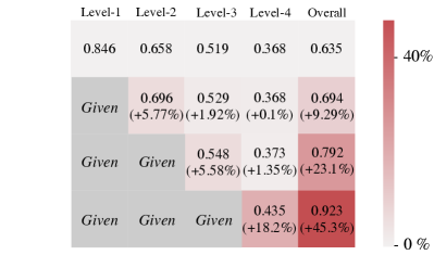
Figure 7: The performance and improvement with given labels in terms of Micro-F1.

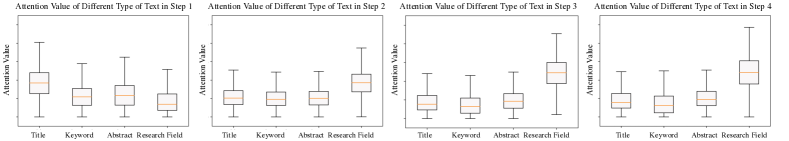
Figure 8: Attention value of different type of semantic information in each step.

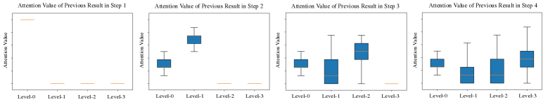
Figure 9: Attention value of historical prediction results in each step.

The Given Labels is a partial label set provided by applicants or funding administrators when they try to fill the ApplyID. As mentioned in the previous section, we hope the HIRPCN can be an assistant who knows the whole picture of the discipline system to aid the categorization with the manager. This study evaluated the improvement when HIRPCN receives incomplete labels and predicts the rest label. It is also worth noting that other baseline methods use a hidden vector to represent previous prediction results, which cannot initialize the prediction from a given partial label set. Thus, we compared the performance of HIRPCN with different levels of provided expert knowledge on the RP-differ dataset. As you can see in Figure 7, the first row of this heatmap showed the Micro-F1 of the HIRPCN on RP-differ when applicants were not given the partial labels. The rest rows illustrated when the first level, first and second level, first, second and third level were given and how the model improved its performance using these partial labels. The color of each cell showed the strength of the improvement. From the heatmap, we can observe that: Firstly, with the incomplete labels given, the overall performance of HIRPCN rises. This phenomenon proves that the architecture enables the model to utilize the partial label to improve the overall performance. Secondly, we noticed that the given partial labels could significantly improve the next-level prediction but decline in the remaining level. We interpret this phenomenon as the current prediction result might be more related to its most recent-level results. So, the model would be trained to raise a high attention on the most current level rather than other earlier-level. In summary, the improvement from the given partial label shows the potential application scenario for the AI assistant system.

4.2.6 RQ6: Attention Mechanism On Information Fusion

Adaptively utilizing each part of the research proposal and the previous prediction results is the most critical idea of the Information Fusion component. In this experiment, we gathered the model’s attention value on each previous prediction step and each different type of text from the IF component. The results was reported in Figure 8 and Figure 9.

The attention to different types of text: Figure 8 illustrated the attention value of the different types of documents in each step. We observed that the Title field is important while predicting the major discipline (step 1). However, HIRPCN will pay more attention to the Research Field and Abstract to generate the rest labels. Although, it might not be noteworthy to interpret and compare the model mechanism with experts’ behavior. But, compared to simply concatenating the text sequence, the attention mechanism could provide more potential for information fusion.

The attention to historical prediction results: Figure 9 showed the model’s attention to the historical prediction results. We noticed that the model would adopt the interdisciplinary knowledge information from the most recent predictions. However, the model might consider other historical predictions to generate the rest in some cases. This phenomenon also proves the experiment observation in RQ5 (i.e., the given partial label will significantly improve the next level’s performance).

To sum up, the attention in the Information Fusion will adaptively variate during the prediction progress. This phenomenon shows the validity of the model component and brings excellent potential to the HIRPCN.

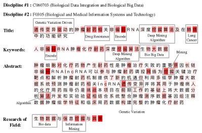
Figure 10: A interdisciplinary research proposal and its word-level attention visualization from the Information Sciences and the Life Sciences.

4.2.7 RQ7: Attention Mechanism On Text

Figure 10 is a case study of an interdisciplinary research proposal. If a word token gained more attention from SIE, it would be shaded redder in this figure. The first observation is that the SIE raised a high signal on the critical words instead of the stop words, even in the long text data. For example, in the Abstract, the term “挖掘” (Mining) and “算法” (Algorithm) generally gained more attention than the word “是” (Is) and “和” (And). We think the attention mechanism will help the HIRPCN learn the importance of each word token and find the critical term to identify the topic path. Further, the attention value was high for the terms relevant to the corresponded discipline of the research proposal. For example, in the Title, the word “肺癌” (Lung Cancer) and “深度挖掘算法” (Deep Mining Algorithm) gained more attention due to they were relevant respectively to the Life Sciences and Information Sciences. This phenomenon shows that the HIRPCN can extract useful semantic information from documents by highlighting domain-related words. Lastly, the self-attention mechanism worked well in the documents with multiple types and variable lengths, such as the term “耐药相关” (Drug Resistance) in the Title or the words “挖掘” (Mining), “算法” (Algorithm) in the Abstract. We believe this phenomenon shows why the SIE is superior for handling the multiple texts in research proposals. In addition, those highlighted critical words can bring interpretability to HIRPCN, which is also essential for fund administrators.

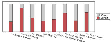
Figure 11: The results of hidden interdiscipline find study.

4.2.8 RQ8: Hidden Interdiscipline Find

Among all the wrong cases in RP-all, the HIRPCN classifies part of non-interdisciplinary research to interdisciplinary, which means except for their labeled discipline, our model predicts an extra discipline. After observing those wrong cases, we noticed that these non-interdisciplinary research proposals were somewhat related to their extra predicted disciplines. To understand this phenomenon, We invited eight fund administrators from NSFC with an insightful understanding and management experience of the eight major disciplines to judge if those extra disciplines can provide helpful information for improving the reviewer assignment. We first group those cases by the extra discipline predicted by HIRPCN. Then we sample 50 research proposals from each group. We send those research proposals to each expert according to the expert’s familiar discipline. If the expert thinks the reviewers from the extra discipline should be considered to supplement the peer-review group, they will mark it as correct, otherwise wrong. We illustrated the percentage of correct of each extra discipline in Figure 11. From the results, we can observe that those experts marked 57% of the samples as correct. Further, all experts commented that the HIRPCN could detect the hidden interdisciplinary research domain. Besides these, some experts commented that although some cases were marked wrong, most of them explicitly use the keywords from the predicted extra discipline. The Experts categorized those cases into non-interdisciplinary research because their focal point is on the labeled discipline instead of the predicted extra one (e.g., a study on Artificial Intelligence might introduce the ideas and terms from Neural Sciences. Still, the neuroscientists might be not suitable to review it). Furthermore, some experts commented that they marked some cases as wrong because the investigators created the labeled discipline to cover the extra discipline topic. So, the labeled discipline is enough to describe the research domain. For example, the discipline Bionics and Artificial Intelligent (C1005) in Life Sciences (C), was created to represented the interdiscipline of Bionics (C10) and Artificial Intelligent (F06).

We randomly picked four proposals and listed them in Figure 12. Applicants manually labeled those proposals with one discipline, but our model extra marked them with another domain from the Information Sciences. We can observe that those research proposals are highly related to their labeled disciplines, while they also strongly bond with the Information Sciences, whether the methodology or the idea. We believe that, with the HIRPCN, those research proposals can be reviewed by experts who are knowledgeable in both areas, thus providing a fair evaluation.

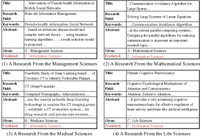
Figure 12: Four cases in different area, while HIRPCN detect another hidden discipline.

4.3 Interdisciplinary Graph Settings

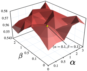
Figure 13: The model performance with different interdisciplinary graph settings.

As mentioned in Section 2.1.4, we introduced a weighted graph to represent the interdisciplinarity between each discipline. This weight is defined by the proportion (disparity) and the citation number (frequency) of the overlap topic in Equation 3. On the one hand, if two domains show high interdisciplinarity, their research area will have great distinction overall, but their overlap topic will be a significant hot area to research. On the other hand, two disciplines that have too many overlapped topics or their overlap topic have little citation might be two similar disciplines (e.g., the Machine Learning and the Deep Learning) or two irrelative areas (e.g., the Management Sciences and the Electronic Engineering), both show little interdisciplinarity. We use two parameter $\alpha$ and $\beta$ to set the weight of two component.

We trained the HIRPCN on RP-differ with different combinations of $\alpha$ and $\beta$. The result of model performance in epoch 100 is visualized in Figure 13. From the figure, we can observe that the best setting of the interdisciplinary graph is set the $\alpha$ and $\beta$ to 0.1. If we both set the $\alpha$ and $\beta$ to 0, all edge weights will equal 1.0, and the graph will deteriorate to a co-topic graph. In epoch 100, this setting would undermine the model performance by around -3.5% compared to the best setting. We believe this phenomenon will explain the importance of interdisciplinary knowledge and our adopted RS measurement.

4.4 Hyperparameter Selection

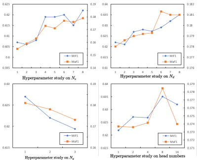
Figure 14: Hyper parameter selection study.

We conducted experiments to evaluate the effect of four key hyperparameters, i.e., $N_{e}$, $N_{d}$, $N_{g}$, and the number of self-attention heads in the SIE and IF. We investigated the sensitivity of those parameters in each part of HIRPCN and reported the results in Figure 14. From the figure, we can observe that with the $N_{e}$ and $N_{d}$ vary from 1 to 8, the performance of HIRPCN increases at first and then decreases slowly. The model will likely be over-fitting to impact the classification results with more parameters introduced. Also, we found that the model would have the best performance when IKE sampled a one-hop neighborhood to extract interdisciplinary knowledge. The reason is that the interdisciplinary graph has many edges, and two or more hop sampling strategies will make the sampled sub-graph denser, which will provide unrelated knowledge for IKE. Lastly, more attention heads will generally improve the performance of HIRPCN. Meanwhile, we found that too many attention heads will make the model performs worse. Based on the experimental result, we set $N_{e}$ to 8, $N_{d}$ to 8, $N_{g}$ to 1, and the number of self-attention heads to 8 to achieve the best performance.

5 Related Works

5.1 Text Classification

The text classification [39] problem is a classical natural language processing task, which aims to extract intrinsic semantic information and assign its related labels. The shallow approaches, such as Word2Vec [16], and GloVe [40], aim to map the word sequence into vector space and then classify each document by this representation. The deep-learning approaches developed many encoders to enhance the semantic information extraction, such as RNN-based [41, 26, 27], CNN-based [22, 28, 23], Attention-based [12], and pretrained language model based [21]. Apart from those approaches, many solutions have been proposed to solve the Multi-label Text Classification, such as WRAP [42], LCBM [43], and 3WDLE [44]. However, in a real-world scenario, the labels of text classification are always exhibit a hierarchical structure, which named the Hierarchical Multi-label Text Classification (HMTC) task. To address this challenge, the study [31] learns the label dependency and uses this dependency to construct the loss function. HiLAP [32] proposed a reinforcement approach so the prediction can follow the label structure. HiAGM [33] proposed two structure encoders for modeling the hierarchical labels. HiMatch [45] implemented a text-to-hierarchical-label matching network. The interdisciplinary research proposal classification task can be seen as a complicated form of HMTC task which aims to categorize multiple types of documents into a hierarchical discipline structure.

5.2 Hierarchical Multi-label Classification

Our work is most related to deep-learning based hierarchical multi-label classification [46] (HMC) methods which leverage standard neural network approaches for multi-label classification problems [47, 29, 48] and then exploit the hierarchy constraint [30] in order to produce coherent predictions and improve performance. Zhang et al. [49] propose a document categorization method with hierarchical structure under weak supervision. The work [50] design a attention-based graph convolution network to category the patent to IPC codes. The work in [51] use the convolution neural network as an encoder and explore the HMC problem in image classification. The works in [52] propose a active learning approach for HMC problem. Aly et al. [53] propose a capsule network based method for HMC problem. TAXOGAN [54] embedding the network nodes and hierarchical labels together, which focuses on taxonomy modeling. In recent studies [55], researchers try to exploit more information among the label embedding and label correlation. Besides the label embedding approach, the study [56] explore the performance of hierarchy dependency as a training constraint and achieve well performance on a small dataset with neural networks. The previous studies in this area are well constructed and have significant success in a specific dataset. However, few studies [36, 57] focus on the complex sci-tech text data classification with a hierarchical discipline structure. In this paper, we inherit the fundamental idea of HMC networks to construct our novel classification methods on the hierarchical discipline structure.

6 Conclusion

This paper proposed HIRPCN, a novel HMC method for the IRPC task on the real-world research proposal dataset. This method extracts the semantic information from each document separately and combines them to achieve a high-level abstraction. Then, the model process each previous level’s prediction result and neighborhood topology structure on the pre-defined interdisciplinary graph as interdisciplinary knowledge. The prediction step integrates each part of the research proposal by attention mechanism and generates the next level prediction. The experiments show that our model achieves the best performance on three real-world datasets and can provide the best granular on each level prediction. Other experiments explains the attention mechanism and points out that our model could fix the incomplete interdisciplinary labels under a domain-specific expert evaluation. With the ability to start prediction from any given label, HIRPCN could assist whether researcher or fund administrator to fill the discipline information, which is crucial to improve the reviewer assignation.

7 Acknowledgments

This work was supported by the Natural Science Foundation of China under Grant No.61836013, the National Key Research and Development Plan of China under Grant No. 2022YFF0712200, Beijing Natural Science Foundation under Grant No.4212030, Youth Innovation Promotion Association, CAS.

Meng Xiao was born in 1995. He received his B.S. degree from the East China University of Technology and graduated from China University of Geosciences (Wuhan) with a master’s degree. He is currently working toward obtaining a Ph.D. degree at the University of Chinese Academy of Sciences. His main research interests include Data Mining, Graph Representation Learning, Hierarchical Multi-label Text Classification combined with the knowledge, and the Knowledge Graphs of the discipline system.

Ziyue Qiao was born in 1996. He received his B.E. degree in 2017 from the Wuhan University, China. He is currently working toward obtaining a Ph.D. degree at the Computer Network Information Center, University of Chinese Academy of Sciences. His research interests include data mining, graph learning, and natural language processing, with an emphasis on designing new algorithms for graph representation/transfer learning and academic data mining.

Yanjie Fu is an assistant professor in the Department of Computer Science at the University of Central Florida. He received his Ph.D. degree from Rutgers, the State University of New Jersey in 2016, the B.E. degree from University of Science and Technology of China in 2008, and the M.E. degree from Chinese Academy of Sciences in 2011. His research interests include data mining and big data analytics.

Hao Dong was born in 1997. He received his B.S. degree in 2019 from Shaanxi Normal University, China. He is currently working toward obtaining a Ph.D. degree at the Computer Network Information Center, University of Chinese Academy of Sciences. His research probes Data Mining, Natural Language Processing, Knowledge-Based Graph, and Temporal Graph.

Yi Du was born in 1988. He received his Ph.D. degree from Institute of Software, Chinese Academy of Sciences in 2013. He is a professor at the Department of Big Data Technology and Application Development at Computer Network Information Center, Chinese Academy of Sciences. His research interests include big data and visual analytics.

Pengyang Wang is an assistant professor in the State Key Lab of Internet of Things and Smart Cities at the University of Macau. He received his Ph.D. in Computer Science from the University of Central Florida. He has broad interests in data mining and machine learning, especially in geospatial-temporal data modeling. He has published in related domains on top venues such as KDD, TKDE, IJCAI, WWW, AAAI etc. He also served as a (senior) program committee member among top conferences in the data mining and artificial intelligence communities.

Hui Xiong is currently a Chair Professor at the Hong Kong University of Science and Technol- ogy (Guangzhou). Dr. Xiong’s research interests include data mining, mobile computing, and their applications in business. Dr. Xiong received his PhD in Computer Science from University of Minnesota, USA. For his outstanding contributions to data mining and mobile computing, he was elected an AAAS Fellow and an IEEE Fellow in 2020.

Yuanchun Zhou was born in 1975. He received his Ph.D. degree from Institute of Computing Technology, Chinese Academy of Sciences, in 2006. He is a professor, Ph.D. supervisor, the deputy director of Computer Network Information Center, Chinese Academy of Sciences. His research interests include data mining, big data processing, and knowledge graph.

References

- [1] S. Milojević, “Quantifying the cognitive extent of science,” Journal of Informetrics, vol. 9, no. 4, pp. 962–973, 2015.
- [2] S. Fortunato, C. T. Bergstrom, K. Börner, J. A. Evans, D. Helbing, S. Milojević, A. M. Petersen, F. Radicchi, R. Sinatra, B. Uzzi et al., “Science of science,” Science, vol. 359, no. 6379, 2018.
- [3] J. G. Foster, A. Rzhetsky, and J. A. Evans, “Tradition and innovation in scientists’ research strategies,” American Sociological Review, vol. 80, no. 5, pp. 875–908, 2015.
- [4] F. Wu, J. Zhang, and V. Honavar, “Learning classifiers using hierarchically structured class taxonomies,” in International symposium on abstraction, reformulation, and approximation. Springer, 2005, pp. 313–320.
- [5] Q. He, “Knowledge discovery through co-word analysis,” Library Trends, vol. 48, no. 1, pp. 133–159, 1999, retrieved from http://eric.ed.gov/?id=EJ595487.
- [6] S. W. Aboelela, E. Larson, S. Bakken, O. Carrasquillo, A. Formicola, S. A. Glied, J. Haas, and K. M. Gebbie, “Defining interdisciplinary research: Conclusions from a critical review of the literature,” Health services research, vol. 42, no. 1p1, pp. 329–346, 2007.
- [7] A. Stirling, “A general framework for analysing diversity in science, technology and society,” Journal of the Royal Society Interface, vol. 4, no. 15, pp. 707–719, 2007.
- [8] A. Porter and I. Rafols, “Is science becoming more interdisciplinary? measuring and mapping six research fields over time,” Scientometrics, vol. 81, no. 3, pp. 719–745, 2009.
- [9] I. Rafols and M. Meyer, “Diversity and network coherence as indicators of interdisciplinarity: case studies in bionanoscience,” Scientometrics, vol. 82, no. 2, pp. 263–287, 2010.
- [10] R. Biggs, M. Schlüter, D. Biggs, E. L. Bohensky, S. BurnSilver, G. Cundill, V. Dakos, T. M. Daw, L. S. Evans, K. Kotschy et al., “Toward principles for enhancing the resilience of ecosystem services,” Annual review of environment and resources, vol. 37, pp. 421–448, 2012.
- [11] C. Winzer, “Conceptualizing energy security,” Energy policy, vol. 46, pp. 36–48, 2012.
- [12] A. Vaswani, N. Shazeer, N. Parmar, J. Uszkoreit, L. Jones, A. N. Gomez, L. Kaiser, and I. Polosukhin, “Attention is all you need,” in Proceedings of the 31st International Conference on Neural Information Processing Systems, vol. 30, 2017, pp. 5998–6008.
- [13] R. Pappagari, P. Zelasko, J. Villalba, Y. Carmiel, and N. Dehak, “Hierarchical transformers for long document classification,” in 2019 IEEE Automatic Speech Recognition and Understanding Workshop (ASRU). IEEE, 2019, pp. 838–844.
- [14] X. Zhang, F. Wei, and M. Zhou, “Hibert: Document level pre-training of hierarchical bidirectional transformers for document summarization,” arXiv preprint arXiv:1905.06566, 2019.
- [15] Y. Liu and M. Lapata, “Hierarchical transformers for multi-document summarization,” arXiv preprint arXiv:1905.13164, 2019.
- [16] T. Mikolov, I. Sutskever, K. Chen, G. S. Corrado, and J. Dean, “Distributed representations of words and phrases and their compositionality,” in Advances in Neural Information Processing Systems 26, vol. 26, 2013, pp. 3111–3119.
- [17] A. Dosovitskiy, L. Beyer, A. Kolesnikov, D. Weissenborn, X. Zhai, T. Unterthiner, M. Dehghani, M. Minderer, G. Heigold, S. Gelly et al., “An image is worth 16x16 words: Transformers for image recognition at scale,” arXiv preprint arXiv:2010.11929, 2020.
- [18] K. Han, A. Xiao, E. Wu, J. Guo, C. Xu, and Y. Wang, “Transformer in transformer,” arXiv preprint arXiv:2103.00112, 2021.
- [19] T. N. Kipf and M. Welling, “Semi-supervised classification with graph convolutional networks,” arXiv preprint arXiv:1609.02907, 2016.
- [20] M. Wang, D. Zheng, Z. Ye, Q. Gan, M. Li, X. Song, J. Zhou, C. Ma, L. Yu, Y. Gai, T. Xiao, T. He, G. Karypis, J. Li, and Z. Zhang, “Deep graph library: A graph-centric, highly-performant package for graph neural networks,” arXiv preprint arXiv:1909.01315, 2019.
- [21] J. Devlin, M.-W. Chang, K. Lee, and K. Toutanova, “Bert: Pre-training of deep bidirectional transformers for language understanding,” arXiv preprint arXiv:1810.04805, 2018.
- [22] P. Bojanowski, E. Grave, A. Joulin, and T. Mikolov, “Enriching Word Vectors with Subword Information,” Transactions of the Association for Computational Linguistics, vol. 5, pp. 135–146, 2017.
- [23] R. Johnson and T. Zhang, “Deep pyramid convolutional neural networks for text categorization,” ACL 2017 - 55th Annual Meeting of the Association for Computational Linguistics, Proceedings of the Conference (Long Papers), vol. 1, pp. 562–570, 2017.
- [24] A. Joulin, E. Grave, P. Bojanowski, and T. Mikolov, “Bag of tricks for efficient text classification,” 15th Conference of the European Chapter of the Association for Computational Linguistics, EACL 2017 - Proceedings of Conference, vol. 2, pp. 427–431, 2017.
- [25] P. Bojanowski, E. Grave, A. Joulin, and T. Mikolov, “Enriching Word Vectors with Subword Information,” Transactions of the Association for Computational Linguistics, vol. 5, pp. 135–146, 2017.
- [26] P. Liu, X. Qiu, and H. Xuanjing, “Recurrent neural network for text classification with multi-task learning,” IJCAI International Joint Conference on Artificial Intelligence, vol. 2016-Janua, pp. 2873–2879, 2016.
- [27] P. Zhou, W. Shi, J. Tian, Z. Qi, B. Li, H. Hao, and B. Xu, “Attention-based bidirectional long short-term memory networks for relation classification,” 54th Annual Meeting of the Association for Computational Linguistics, ACL 2016 - Short Papers, pp. 207–212, 2016.
- [28] P. Bojanowski, E. Grave, A. Joulin, and T. Mikolov, “Enriching Word Vectors with Subword Information,” Transactions of the Association for Computational Linguistics, vol. 5, pp. 135–146, 2017.
- [29] J. Wehrmann, R. Cerri, and R. Barros, “Hierarchical multi-label classification networks,” in International Conference on Machine Learning. PMLR, 2018, pp. 5075–5084.
- [30] W. Huang, E. Chen, Q. Liu, Y. Chen, Z. Huang, Y. Liu, Z. Zhao, D. Zhang, and S. Wang, “Hierarchical multi-label text classification: An attention-based recurrent network approach,” in Proceedings of the 28th ACM International Conference on Information and Knowledge Management, 2019, pp. 1051–1060.
- [31] H. Peng, J. Li, S. Wang, L. Wang, Q. Gong, R. Yang, B. Li, P. Yu, and L. He, “Hierarchical taxonomy-aware and attentional graph capsule rcnns for large-scale multi-label text classification,” IEEE Transactions on Knowledge and Data Engineering, 2019.
- [32] Y. Mao, J. Tian, J. Han, and X. Ren, “Hierarchical text classification with reinforced label assignment,” arXiv preprint arXiv:1908.10419, 2019.
- [33] J. Zhou, C. Ma, D. Long, G. Xu, N. Ding, H. Zhang, P. Xie, and G. Liu, “Hierarchy-aware global model for hierarchical text classification,” in Proceedings of the 58th Annual Meeting of the Association for Computational Linguistics, 2020, pp. 1106–1117.
- [34] E. Gibaja and S. Ventura, “Multi-label learning: a review of the state of the art and ongoing research,” Wiley Interdisciplinary Reviews: Data Mining and Knowledge Discovery, vol. 4, no. 6, pp. 411–444, 2014.
- [35] C. Vens, J. Struyf, L. Schietgat, S. Džeroski, and H. Blockeel, “Decision trees for hierarchical multi-label classification,” Machine learning, vol. 73, no. 2, p. 185, 2008.
- [36] M. Xiao, Z. Qiao, Y. Fu, Y. Du, and P. Wang, “Expert knowledge-guided length-variant hierarchical label generation for proposal classification,” 2021 IEEE International Conference on Data Mining, pp. 757–766, 2021.
- [37] D. P. Kingma and J. Ba, “Adam: A method for stochastic optimization,” arXiv preprint arXiv:1412.6980, 2014.
- [38] A. Paszke, S. Gross, F. Massa, A. Lerer, J. Bradbury, G. Chanan, T. Killeen, Z. Lin, N. Gimelshein, L. Antiga et al., “Pytorch: An imperative style, high-performance deep learning library,” arXiv preprint arXiv:1912.01703, 2019.
- [39] Q. Li, H. Peng, J. Li, C. Xia, R. Yang, L. Sun, P. S. Yu, and L. He, “A survey on text classification: From shallow to deep learning,” arXiv preprint arXiv:2008.00364, 2020.
- [40] J. Pennington, R. Socher, and C. D. Manning, “Glove: Global vectors for word representation,” in Proceedings of the 2014 conference on empirical methods in natural language processing (EMNLP), 2014, pp. 1532–1543.
- [41] S. Hochreiter and J. Schmidhuber, “Long short-term memory,” Neural computation, vol. 9, no. 8, pp. 1735–1780, 1997.
- [42] Z.-B. Yu and M.-L. Zhang, “Multi-label classification with label-specific feature generation: A wrapped approach,” IEEE Transactions on Pattern Analysis and Machine Intelligence, 2021.
- [43] S. Sun and D. Zong, “Lcbm: a multi-view probabilistic model for multi-label classification,” IEEE Transactions on Pattern Analysis and Machine Intelligence, vol. 43, no. 8, pp. 2682–2696, 2020.
- [44] T. Zhao, Y. Zhang, D. Miao, and W. Pedrycz, “Selective label enhancement for multi-label classification based on three-way decisions,” International Journal of Approximate Reasoning, vol. 150, pp. 172–187, 2022.
- [45] H. Chen, Q. Ma, Z. Lin, and J. Yan, “Hierarchy-aware label semantics matching network for hierarchical text classification,” in Proceedings of the 59th Annual Meeting of the Association for Computational Linguistics and the 11th International Joint Conference on Natural Language Processing (Volume 1: Long Papers), 2021, pp. 4370–4379.
- [46] R. Cerri, R. C. Barros, and A. C. de Carvalho, “Hierarchical classification of gene ontology-based protein functions with neural networks,” in 2015 international joint conference on neural networks (IJCNN). IEEE, 2015, pp. 1–8.
- [47] E. Giunchiglia and T. Lukasiewicz, “Multi-label classification neural networks with hard logical constraints,” arXiv preprint arXiv:2103.13427, 2021.
- [48] F. Gargiulo, S. Silvestri, M. Ciampi, and G. De Pietro, “Deep neural network for hierarchical extreme multi-label text classification,” Applied Soft Computing, vol. 79, pp. 125–138, 2019.
- [49] Y. Zhang, X. Chen, Y. Meng, and J. Han, “Hierarchical metadata-aware document categorization under weak supervision,” in Proceedings of the 14th ACM International Conference on Web Search and Data Mining, 2021, pp. 770–778.
- [50] P. Tang, M. Jiang, B. N. Xia, J. W. Pitera, J. Welser, and N. V. Chawla, “Multi-label patent categorization with non-local attention-based graph convolutional network,” in Proceedings of the AAAI Conference on Artificial Intelligence, vol. 34, no. 05, 2020, pp. 9024–9031.
- [51] R. La Grassa, I. Gallo, and N. Landro, “Learn class hierarchy using convolutional neural networks,” Applied Intelligence, pp. 1–7, 2021.
- [52] F. K. Nakano, R. Cerri, and C. Vens, “Active learning for hierarchical multi-label classification,” Data Mining and Knowledge Discovery, vol. 34, no. 5, pp. 1496–1530, 2020.
- [53] R. Aly, S. Remus, and C. Biemann, “Hierarchical multi-label classification of text with capsule networks,” ACL 2019 - 57th Annual Meeting of the Association for Computational Linguistics, Proceedings of the Student Research Workshop, pp. 323–330, 2019.
- [54] C. Yang, J. Zhang, and J. Han, “Co-embedding network nodes and hierarchical labels with taxonomy based generative adversarial networks,” Proceedings - IEEE International Conference on Data Mining, ICDM, vol. 2020-Novem, pp. 721–730, 2020.
- [55] H. Liu, G. Chen, P. Li, P. Zhao, and X. Wu, “Multi-label text classification via joint learning from label embedding and label correlation,” Neurocomputing, vol. 460, pp. 385–398, 2021.
- [56] E. Giunchiglia and T. Lukasiewicz, “Coherent hierarchical multi-label classification networks,” Advances in Neural Information Processing Systems, vol. 33, pp. 9662–9673, 2020.
- [57] M. Xiao, M. Wu, Z. Qiao, Z. Ning, Y. Du, Y. Fu, and Y. Zhou, “Hierarchical mixup multi-label classification with imbalanced interdisciplinary research proposals,” arXiv preprint arXiv:2209.13912, 2022.