Rotating Solar Models in Agreement with Helioseismic Results and Updated Neutrino Fluxes

Abstract

Standard solar models (SSMs) constructed in accordance with old solar abundances are in reasonable agreement with seismically inferred results, but SSMs with new low-metal abundances disagree with the seismically inferred results. The constraints of neutrino fluxes on solar models exist in parallel with those of helioseismic results. The solar neutrino fluxes were updated by Borexino Collaboration. We constructed rotating solar models with new low-metal abundances where the effects of enhanced diffusion and convection overshoot were included. A rotating model using OPAL opacities and the Caffau abundance scale has better sound-speed and density profiles than the SSM with the old solar abundances and reproduces the observed $p$-mode frequency ratios $r_{02}$ and $r_{13}$. The depth and helium abundance of the convection zone of the model agree with the seismically inferred ones at the level of $1\sigma$. The updated neutrino fluxes are also reproduced by the model at the level of $1\sigma$. The effects of rotation and enhanced diffusion not only improve the model’s sound-speed and density profiles but bring the neutrino fluxes predicted by the model into agreement with the detected ones. Moreover, the calculations show that OP may underestimate opacities for the regions of the Sun with $T\gtrsim 5\times 10^{6}$ K by around $1.5\%$, while OPAL may underestimate opacities for the regions of the Sun with $2\times 10^{6}$ K $\lesssim T\lesssim 5\times 10^{6}$ K by about $1-2\%$.

1 Introduction

The heavy-element abundance $Z_{s}$ of the Sun, derived by Grevesse & Sauval (1998, hereafter GS98) from photospheric spectroscopy, is $0.017$, whose uncertainty is of the order of $10$ percent. The ratio of the heavy-element abundance to hydrogen abundance is $0.0231$. Since Lodders (2003) and Asplund et al. (2005) reassessed the value of the $Z_{s}$, it has been revised several times (Lodders et al., 2009; Asplund et al., 2009; Caffau et al., 2010, 2011; Lodders, 2020; Asplund et al., 2021; Amarsi et al., 2021). The well-known values of the new $Z_{s}$ are $0.0133$ (Lodders, 2003), $0.0122$ (Asplund et al., 2005), $0.0141$ (Lodders et al., 2009), or $0.0134$ (Asplund et al., 2009, hereafter AGSS09). These revised values are obviously lower than the old one.

The helium abundance, $Y_{s}$, in the solar convection zone (CZ) and thus photosphere cannot be inferred directly from spectroscopy, but can be determined by helioseismology. The values of seismically inferred $Y_{s}$ and $Z_{s}$ are $0.2485\pm 0.0035$ (Basu & Antia, 2004; Serenelli & Basu, 2010) and $0.0172\pm 0.002$ (Antia & Basu, 2006), respectively. However, the values given by Vorontsov et al. (2013) or Vorontsov et al. (2014) are in the range of $Y_{s}=0.240–0.255$ and $Z_{s}=0.008–0.013$ or $Y_{s}=0.245–0.260$ and $Z_{s}=0.006–0.011$. Moreover, the value of $Z_{s}$ inferred by Buldgen et al. (2017) is in the range of $0.008–0.014$. The radius of the base of the CZ (BCZ) also can be determined by helioseismology. The inferred radius of the BCZ is $0.713\pm 0.003$ $R_{\odot}$ (Christensen-Dalsgaard et al., 1991) or $0.713\pm 0.001$ $R_{\odot}$ (Basu & Antia, 1997).

The standard solar models (SSMs) constructed in accordance with the high metal abundances (old solar abundances, e.g. GS98) are considered to be in good agreement with the seismically inferred sound-speed and density profiles, depth and helium abundance of the CZ, but the SSMs constructed in accordance with the low metal abundances (revised solar abundances) do not completely agree with the seismically inferred results (Bahcall et al., 2004; Basu & Antia, 2004; Yang & Bi, 2007; Basu et al., 2009; Serenelli et al., 2009, 2011; Zhang & Li, 2012) and the neutrino flux constraints (Bahcall & Pinsonneault, 2004; Turck-Chièze et al., 2010, 2011; Turck-Chièze & Couvidat, 2011; Yang, 2016), which is known as solar modeling problem or solar abundance problem (Basu et al., 2015; Christensen-Dalsgaard, 2021; Salmon et al., 2021; Amarsi et al., 2021).

In order to reconcile the low-Z models with helioseismology, many physical effects have been studied. For example, increased opacity at the base of the CZ was studied by Bahcall et al. (2004), Serenelli et al. (2009), and Buldgen et al. (2019); enhanced neon abundance was suggested by Bahcall et al. (2005); mass accretion of metal-rich/poor material or helium-poor material was investigated by Castro et al. (2007), Guzik & Mussack (2010), Serenelli et al. (2011), and Zhang et al. (2019); overshooting below the CZ was used to recover the CZ depth (Montalbán et al., 2006; Castro et al., 2007; Yang, 2019; Zhang et al., 2019).

In order to match the seismically inferred sound-speed and density profiles (Basu et al., 2000, 2009), the gravitational settling that reduces the surface helium abundance by about $11\%$ ($\sim 0.03$ by mass fraction) below its initial value is required in SSMs. Macroscopic turbulent mixing can reduce the amount of surface helium settling by around $40\%$ (Proffitt & Michaud, 1991). The effects of the turbulent mixing on the diffusion and settling of helium and heavy elements were not considered in the diffusion coefficients of Thoul et al. (1994). Asplund et al. (2004) suggested that enhanced diffusion and settling of helium and heavy elements might be able to reconcile the low-Z models with helioseismology. The increased diffusion can significantly improve sound-speed and density profiles, but leaves the CZ helium abundance too low (Basu & Antia, 2004; Montalbán et al., 2004; Guzik et al., 2005; Yang, 2019).

Rotational mixing can transport helium outward. It thus can counteract the effect of enhanced diffusion on the surface helium abundance (Yang, 2019), i.e., it can improve the prediction of the surface helium abundance. The effects of rotation on the low-Z models were studied by Yang & Bi (2007), Turck-Chièze et al. (2010, 2011), and Yang (2016, 2019). However, the rotating models with AGSS09 mixtures (Yang, 2019) disagree with the detected neutrino fluxes of Borexino Collaboration (2018, 2020).

Bahcall & Pinsonneault (2004) and Serenelli et al. (2009) found that an $11\%-20\%$ increase in OPAL opacities at the BCZ can reconcile the low-Z models with helioseismology. Badnell et al. (2005) showed that in the region OP opacity is slightly larger than OPAL opacity but no more than $2.5$ percent. Buldgen et al. (2019) concluded that the solar modeling problem likely occurs from multiple small contributors. Opacity could be one of the contributors.

The production of solar neutrinos is sensitive to the central properties of the Sun. The ⁸B neutrino flux is strongly dependent on the central temperature of the Sun (Bahcall & Ulrich, 1988; Turck-Chièze & Couvidat, 2011). The determinations of solar neutrino fluxes complement helioseismology in diagnosing the core of the Sun. The constraints of neutrino fluxes on solar models exist in parallel with those of helioseismology and are studied by many authors (Bahcall & Pinsonneault, 2004; Turck-Chièze et al., 2010, 2011; Turck-Chièze & Couvidat, 2011; Yang, 2016, 2019; Zhang et al., 2019). Borexino Collaboration (2018, 2020) updated solar neutrino fluxes and determined the total fluxes of ¹³N, ¹⁵O, and ¹⁷F neutrinos. Their ⁸B neutrino flux is higher than that determined by Bergström et al. (2016). The low-Z model of Zhang et al. (2019) with helium-poor accretion and solar-wind mass loss agrees with helioseismic results but disagrees with the neutrino fluxes detected by Borexino Collaboration (2018, 2020). Moreover, Salmon et al. (2021) showed that the updated solar neutrino fluxes prefer high-metallicity solar models. The solar modeling problem has persisted for almost 20 years.

Caffau et al. (2010, 2011) independently analysed carbon, nitrogen, and oxygen abundances in the solar photosphere. They found that the heavy-element abundance of the solar surface is $Z_{s}=0.0154/0.0153$, supplemented with data from Lodders et al. (2009). The value of $Z_{s}/X_{s}$ advocated by Caffau et al. (2011) is $0.0209$. These values are larger than those of Lodders et al. (2009) and AGSS09. Hope et al. (2020) studied the possible origin of the solar abundance problem. Their result favors the solar $Z_{s}$ reported by Caffau et al. (2011) rather than the measurement by AGSS09.

Lodders (2020) reanalysed the solar photospheric abundances and recommended $Z_{s}=0.0149$ and $Z_{s}/X_{s}=0.0201$. Asplund et al. (2021, hereafter AAG21) also reassessed the solar abundances with updated atomic data and a 3D radiative-hydrodynamical model of the solar photosphere. They advocated $Z_{s}=0.0139\pm 0.0006$, $Y_{s}=0.2423\pm 0.0054$, and $Z_{s}/X_{s}=0.0187\pm 0.0009$. Moreover, using the 3D radiative-hydrodynamical model of solar photosphere, Amarsi et al. (2021) analysed $408$ molecular lines of C, N, and O and obtained solar C, N, and O abundances, which are slightly larger than their previous results in AAG21. With these molecular abundances, the value of the heavy-element abundance of the solar surface increases from $Z_{s}=0.0139$ to $Z_{s}=0.0142$ (Amarsi et al., 2021). This increase indicates that “it may be worthwhile to continue improving the atomic and molecular data as well as the model atmospheres and line formation methods” (Amarsi et al., 2021).

In this work, we mainly focus on whether the solar models constructed in accordance with AAG21 mixtures and Caffau et al. (2011) mixtures agree with the seismically inferred results and updated neutrino fluxes. The paper is organized as follows. Input physics in models are introduced in Section 2, calculation results are presented in Section 3, and discussion and summary are given in Section 4.

2 Input Physics in Models

All solar models were calculated by using the Yale Rotating Stellar Evolution Code (Pinsonneault et al., 1989; Yang & Bi, 2007; Demarque et al., 2008) in its rotation and non-rotation configurations. The frequencies of $p$-modes of models were computed by using the Guenther (1994) pulsation code. The OPAL equation-of-state (EOS2005) tables (Rogers & Nayfonov, 2002), OPAL (Iglesias & Rogers, 1996) and OP opacity tables (Seaton, 1987; The Opacity Project Team, 1995; Badnell et al., 2005; Delahaye et al., 2016) were used, supplemented by the Ferguson et al. (2005) opacity tables at low temperature. The opacity tables were reconstructed with the GS98, Caffau et al. (2011), and AAG21 mixtures (see Appendix A). The nuclear reaction rates were calculated with the subroutine of Bahcall & Pinsonneault (1992) and Bahcall et al. (1995, 2001) (see Appendix B). Convection was determined by the Schwarzschild criterion and treated according to the standard mixing-length theory (Böhm-Vitense, 1958; Kippenhahn et al., 2012). The overshoot region below the BCZ was assumed to be both fully mixed and adiabatically stratified (Christensen-Dalsgaard et al., 1991). The depth of the overshoot region is determined by $\delta_{\rm ov}H_{p}$ (Demarque et al., 2008), where $\delta_{\rm ov}$ is a free parameter and $H_{p}$ is the local pressure scale height. A convection overshoot of $\delta_{\rm ov}\approx 0.1$ is required to recover the seismically inferred depth of the CZ in our rotating models. The diffusion and settling of both helium and heavy elements were computed using the formulas of Thoul et al. (1994). In the atmosphere, Krishna Swamy (1966) $T-\tau$ relation was adopted.

We treated the transport of angular momentum and material mixing as a diffusion process (Endal & Sofia, 1978), i.e.

$$\frac{\partial\Omega}{\partial t}=f_{\Omega}\frac{1}{\rho r^{4}}\frac{\partial}{\partial r}(\rho r^{4}D\frac{\partial\Omega}{\partial r})\,$$ (1)

for the transport of angular momentum and

$$\begin{array}[]{lll}\frac{\partial X_{i}}{\partial t}&=&f_{c}f_{\Omega}\frac{1}{\rho r^{2}}\frac{\partial}{\partial r}(\rho r^{2}D\frac{\partial X_{i}}{\partial r})\\ &&+(\frac{\partial X_{i}}{\partial t})_{\rm nuc}-\frac{1}{\rho r^{2}}\frac{\partial}{\partial r}(f_{0}\rho r^{2}X_{i}V_{i})\end{array}$$ (2)

for the change in the mass fraction $X_{i}$ of chemical species $i$, where $D$ is the diffusion coefficient caused by rotational instabilities including the Eddington circulation, the Goldreich-Schubert-Fricke instability (Pinsonneault et al., 1989), and the secular shear instability of Zahn (1993). The default values of $f_{\Omega}$ and $f_{c}$ are $1$ and $0.03$ (Yang, 2019), respectively. We applied a straight multiplier $f_{0}$ to the diffusion velocity $V_{i}$ to enhance the rates of diffusion and settling, as Basu & Antia (2004), Montalbán et al. (2004), Guzik et al. (2005), and Yang (2019) have done, despite the fact that there is no obvious physical justification for such a multiplier. The value of $f_{0}$ is $1$ for standard cases but larger than $1$ for an enhanced diffusion model. The angular-momentum loss from the CZ due to magnetic braking was calculated with Kawaler’s relation (Kawaler, 1988; Chaboyer et al, 1995). More details of calculation for rotation were described in Pinsonneault et al. (1989) and Yang (2019).

All models were evolved from a homogeneous zero-age main-sequence model to the present solar age $4.57$ Gyr, luminosity $3.844\times 10^{33}$ erg $\mathrm{s}^{-1}$, radius $6.9598\times 10^{10}$ cm, and mass $1.9891\times 10^{33}$ g (Bahcall et al., 1995). The initial metallicity $Z_{0}$, hydrogen abundance $X_{0}$, and mixing-length parameter $\alpha_{\rm{MLT}}$ are free parameters. They were adjusted to match the constraints of luminosity and radius within around $10^{-5}$ and observed $Z_{s}/X_{s}$. The initial helium abundance is determined by $Y_{0}=1-X_{0}-Z_{0}$. The value of $\alpha_{\rm{MLT}}$ changes with input physics, i.e. a new solar calibration of $\alpha_{\rm{MLT}}$ is performed each time the input physics change. The initial rotation rate, $\Omega_{i}$ of rotating models was adjusted to reproduce the solar equatorial velocity of about $2.0$ km s^-1. The values of these parameters are shown in Table 1.

3 Calculation Results

3.1 Solar Models with High Metal Abundances

3.1.1 The Models Constructed with OPAL Opacity Tables

Using the OPAL opacity tables constructed with GS98 mixtures, we computed SSM GS98M and rotating model GS98Mr. The central temperature and density, surface helium and heavy-element abundances, radius of the BCZ, and other parameters of the models are listed in Table 1. The fluxes of $pp$, $pep$, $hep$, ⁷Be, ⁸B, ¹³N, ¹⁵O, and ¹⁷F neutrinos calculated from the models are given in Table 2. Table 3 lists some of the physical configurations of each model.

The surface heavy-element abundance of $0.0174$ of GS98M is in agreement with that determined by GS98. The surface helium abundance and $r_{cz}$ of GS98M are also consistent with the seismically inferred ones (see Table 1). We compared the sound speed and density of models with those inferred by Basu et al. (2009) using the data from the Birmingham Solar-Oscillations Network (Chaplin et al., 1996) and the Michelson Doppler Imager (Schou et al., 1998). The values of relative sound-speed difference, $\delta c_{s}/c_{s}$, and density difference, $\delta\rho/\rho$, between the Sun and GS98M are less than $0.0043$ and $0.028$, respectively (see Figure 1). Moreover, the ratios of small to large frequency separations, $r_{02}$ and $r_{13}$ (Roxburgh & Vorontsov, 2003), of the model agree with those calculated from observed frequencies of Chaplin et al. (1999) or García et al. (2011) (see Figure 2). Table 4 gives the values of $\chi^{2}_{c_{s}+\rho}$ and $\chi^{2}_{d_{02+13}}$ of the models.

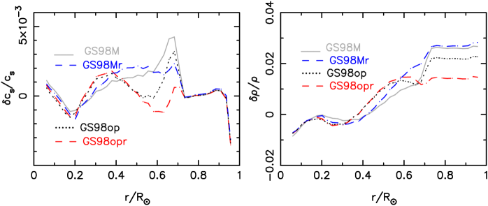
Figure 1: Relative sound-speed and density differences, in the sense (Sun-Model)/Model, between the Sun and models. The solar sound speed and density are given in Basu et al. (2009).

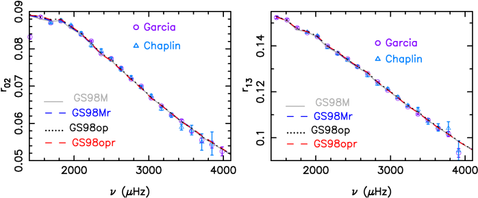
Figure 2: Distributions of observed and predicted ratios $r_{02}$ and $r_{13}$ as a function of frequency. The circles and triangles show the ratios calculated from the frequencies observed by GOLF & VIRGO (García et al., 2011) and BiSON (Chaplin et al., 1999), respectively.

We compared the neutrino fluxes computed from models with those determined by different authors (Bellini et al., 2011, 2012; Ahmed et al., 2004; Bergström et al., 2016; Borexino Collaboration, 2018, 2020) and ones predicted by the models BP04 (Bahcall & Pinsonneault, 2004) and SSeM (Turck-Chièze & Couvidat, 2011) in Table 2. The neutrino fluxes of GS98M are comparable with those of BP04. Some differences between the nuclear cross-section factors $S_{0}$ (Bahcall, 1989) used in BP04 and those used in GS98M are listed in Table 6 of Appendix B. The total fluxes of ¹³N, ¹⁵O, and ¹⁷F neutrinos calculated from GS98M are $\Phi(\rm CNO)=10.2\times 10^{8}$ cm^-2 s^-1, slightly larger than $7^{+3}_{-2}\times 10^{8}$ cm^-2 s^-1 detected by Borexino Collaboration (2020). The $pp$, $pep$, $hep$, ⁷Be, and ⁸B neutrino fluxes of GS98M are in agreement with those determined by Borexino Collaboration (2018). However, the fluxes of ⁷Be and ⁸B neutrinos are larger than those determined by Bergström et al. (2016) (see Table 2).

Figure 1 shows that the effects of rotation can significantly improve the sound-speed and density profiles. The value of the relative sound-speed difference, $\delta c_{s}/c_{s}$, below the CZ can be decreased by about $50\%$. Moreover, the centrifugal effect leads to a decrease in the central temperature. The fluxes of ⁷Be, ⁸B, ¹³N, ¹⁵O, and ¹⁷F neutrinos are sensitive to the central temperature. Thus the fluxes calculated from rotating models are generally lower than those computed from non-rotating models (see Table 2). The total fluxes of ¹³N, ¹⁵O, and ¹⁷F neutrinos of GS98Mr are $\Phi(\rm CNO)=9.5\times 10^{8}$ cm^-2 s^-1, which are in agreement with the detected value of $7^{+3}_{-2}\times 10^{8}$ cm^-2 s^-1. The ⁸B neutrino flux of $5.29\times 10^{6}$ cm^-2 s^-1 for GS98Mr is consistent with $5.16^{+0.13}_{-0.09}\times 10^{6}$ cm^-2 s^-1 determined by Bergström et al. (2016) and $5.68^{+0.39}_{-0.41}\times 10^{6}$ cm^-2 s^-1 detected by Borexino Collaboration (2018). However, the surface helium abundance of 0.2534 of GS98Mr is higher than the inferred value of $0.2485\pm 0.0035$. Thus the high-Z models constructed with OPAL opacities do not completely agree with helioseismic results and updated neutrino fluxes.

3.1.2 The Models Constructed with OP Opacity Tables

In order to study the effects of opacities, we constructed SSM GS98op and rotating model GS98opr by using OP opacity tables. Tables 1 and 2 list the fundamental parameters and neutrino fluxes of the models, respectively. For almost the same metallicity, OP opacities are larger by about $0-2\%$ than OPAL opacities in the region of the Sun with $0.5$ $R_{\odot}$$\lesssim r\lesssim 0.8$ $R_{\odot}$ but smaller by about $1-2\%$ in the region with $r\lesssim 0.4$ $R_{\odot}$ (see Figure 3). The sound-speed and density profiles and frequency separation ratios of the models are shown in Figures 1 and 2, respectively, which show that OP has almost no improvement in the reproduction of the frequency separation ratios in comparison to OPAL (see Figure 2), but obviously improves density profile and the sound-speed profile below the CZ where OP opacities are mainly larger than OPAL opacities. OP slightly worsens the sound-speed profile in the inner layers of radiative region where OP opacities are lower than OPAL opacities (see Figures 1 and 3).

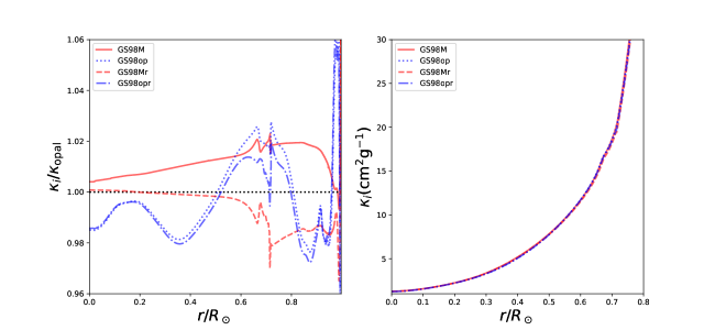
Figure 3: Left panel: comparison of Rosseland mean opacity of different models relative to that of a reference model constructed with OPAL opacity tables and $Z_{s}=0.0170$. Right panel: distributions of Rosseland mean opacity of the models as a function of radius.

In order to obtain the same surface heavy-element abundance and the solar luminosity and radius at the age of $4.57$ Gyr, the decrease in opacities requires decreasing the initial helium abundance and changing $\alpha_{\rm{MLT}}$. As a consequence, the surface helium abundances of the models constructed with OP opacity tables are lower than those of the models constructed with OPAL opacity tables. The surface helium abundance of $0.2414$ for GS98op is smaller than the inferred value of $0.2485\pm 0.0035$. Therefore, GS98op is not a good SSM.

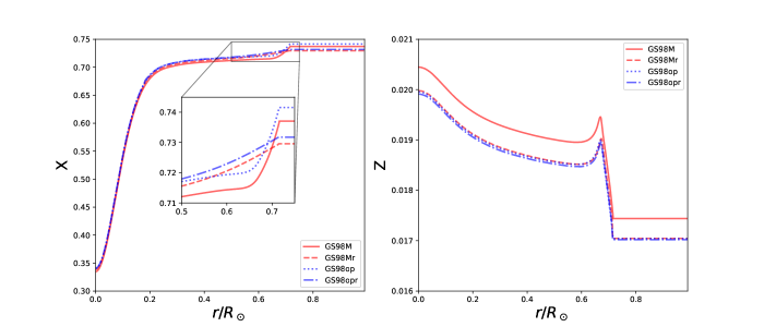
Figure 4: Distributions of hydrogen and metal abundances of models as a function of radius.

Rotational mixing brings hydrogen into inner layers from outer layers and transports helium outward, i.e. decreases the hydrogen abundance in the CZ, but increases the hydrogen abundance in the region with $0.5$ $R_{\odot}$ $\lesssim r\lesssim 0.7$ $R_{\odot}$ (see Figure 4), which changes the distribution of the mean molecular weight. As a consequence, the density and sound-speed profiles are significantly improved by the effects of rotation. The value of the relative sound-speed difference below the CZ is decreased by about $80\%$ (see Figure 1). Although OP improves the sound-speed profile below the CZ, the effects of rotation play a more important role in improving the sound-speed profile. Moreover, the amount of the CZ helium settling is reduced by about $34\%$. The surface helium abundance of $0.2511$ for GS98opr is in agreement with the seismically inferred value of $0.2485\pm 0.0035$, and increased by about $0.01$ compared to that of the non-rotating model.

The central temperatures of models constructed with OP opacity tables are lower than those of models constructed with OPAL opacity tables. Therefore, the fluxes of ⁷Be, ⁸B, ¹³N, ¹⁵O, and ¹⁷F neutrinos computed from GS98op and GS98opr are smaller than those calculated from GS98M and GS98Mr. The total fluxes $\Phi(\rm CNO)$ of GS98op and GS98opr are in agreement with that detected by Borexino Collaboration (2020). The ⁸B neutrino fluxes of the models are consistent with that determined by Bergström et al. (2016) but lower than one detected by Borexino Collaboration (2018). Thus the high-Z models constructed with OP opacities also do not completely agree with helioseismic results and updated neutrino fluxes.

We chose GS98M as the best SSM and GS98opr as the best rotating model with high metal abundances and went on to construct the models with low metal abundances and compare them with these two models.

3.2 Solar Models with Low Metal Abundances

3.2.1 Standard and Rotating Models

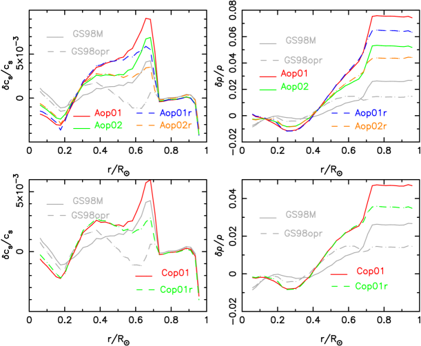
Figure 5: Relative sound-speed and density differences, in the sense (Sun-Model)/Model, between the Sun and models. The solar sound speed and density are given in Basu et al. (2009).

Using OP opacity tables reconstructed with AAG21 mixtures, we computed SSM Aop01 and rotating model Aop01r with the surface heavy-element abundance determined by Asplund et al. (2021). Although OP opacities and the effects of rotation can significantly improve sound-speed and density profiles, the sound-speed and density profiles of Aop01 and Aop01r are not as good as those of GS98M (see Figure 5). The models also can not reproduce the observed frequency separation ratios $r_{02}$ and $r_{13}$ (see Figure 6 or Table 4) and inferred helium abundance. The total fluxes $\Phi(\rm CNO)$ of Aop01 and Aop01r are in agreement with the detection of Borexino Collaboration (2020), but their ⁷Be and ⁸B neutrino fluxes are too low (see Table 2).

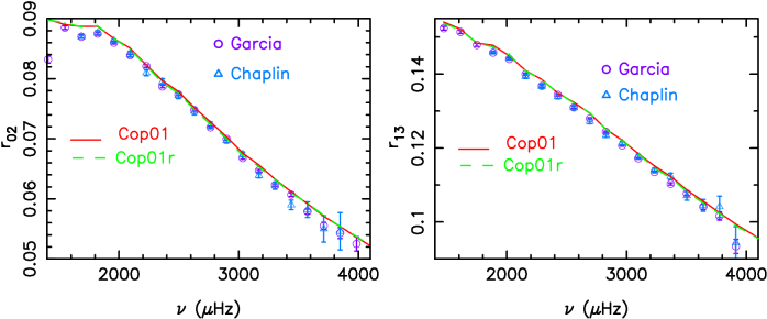
Figure 6: Distributions of observed and predicted ratios $r_{02}$ and $r_{13}$ as a function of frequency. The circles and triangles show the ratios calculated from the frequencies observed by GOLF & VIRGO (García et al., 2011) and BiSON (Chaplin et al., 1999), respectively.

With the heavy-element abundance determined by Lodders (2020), we constructed SSM Aop02 and rotating model Aop02r. We also calculated SSM Cop01 and rotating model Cop01r by using the OP opacity tables reconstructed with Caffau et al. (2011) mixtures. The SSMs Aop02 and Cop01 obviously disagree with seismically inferred results and detected ⁸B neutrino flux. For rotating models Aop02r and Cop01r, the overshoot of convection brings the depth of the CZ into agreement with the seismically inferred one. The surface helium abundances of Aop02r and Cop01r are $0.2453$ and $0.2467$, respectively, consistent with the inferred value of $0.2485\pm 0.0035$. The total fluxes $\Phi(\rm CNO)$ predicted by Aop02r and Cop01r are $7.4$ and $7.6\times 10^{8}$ cm^-2 s^-1, respectively, which are in good agreement with that detected by Borexino Collaboration (2020). The sound-speed profiles of Aop02r and Cop01r are comparable with that of GS98M (see Figure 5). The observed frequency separation ratios $r_{02}$ and $r_{13}$ are almost reproduced by the models (see Figure 6). However, the ⁸B neutrino fluxes of Aop02r and Cop01r are obviously lower than those determined by Bergström et al. (2016) and Borexino Collaboration (2018) (see Table 2). Moreover, their density profiles are not as good as that of GS98M. These indicate that the effects of OP and rotation can improve the solar model but can not completely solve the solar modeling problem.

3.2.2 Rotating and Enhanced Diffusion Models Constructed in Accordance with AAG21 Mixtures

The gravitational settling and diffusion reduce the surface helium abundance of SSMs by around $11\%$ ($\sim 0.03$ by mass fraction) below its initial value (see Table 1), which plays an important role in shaping the sound-speed and density profiles of the models. Rotational mixing reduces the amount of the surface helium settling by about $33\%-36\%$. In order to counteract the effects of rotational mixing on the settling of elements, we increased the rates of element diffusion and settling by $36\%$, and then constructed rotating models Aop12r and Aopal12r by using OP and OPAL opacity tables. The two models had the surface heavy-element abundance determined by Lodders (2020). Tables 1 and 2 list their fundamental parameters and neutrino fluxes, respectively.

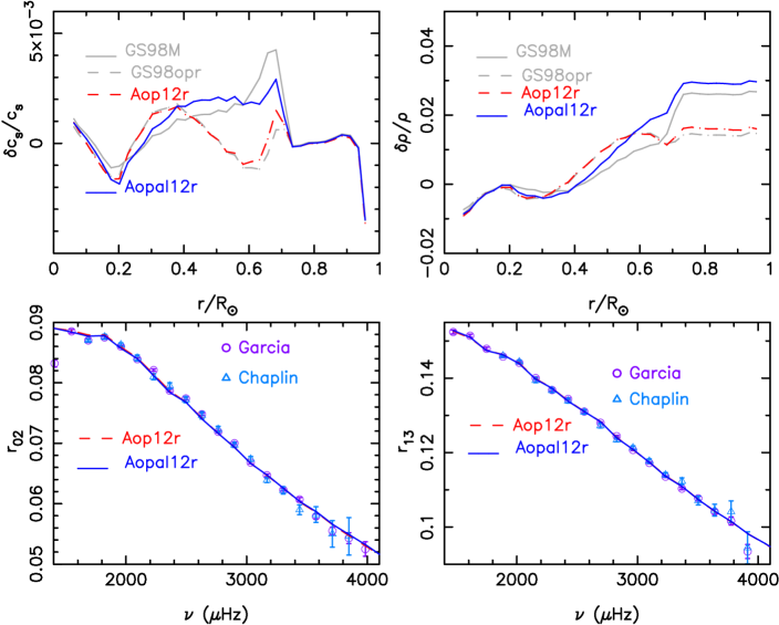
Figure 7: Top panels: relative sound-speed and density differences, in the sense (Sun-Model)/Model, between the Sun and models. The solar sound speed and density are given in Basu et al. (2009). Bottom panels: distributions of observed and predicted ratios $r_{02}$ and $r_{13}$ as a function of frequency. The circles and triangles show the ratios calculated from the frequencies observed by GOLF & VIRGO (García et al., 2011) and BiSON (Chaplin et al., 1999), respectively.

The sound-speed and density profiles of Aopal12r are almost as good as those of GS98M, but those of Aop12r are obviously better than those of GS98M (see Figure 7). The inferred CZ depth and observed frequency separation ratios $r_{02}$ and $r_{13}$ are reproduced well by the two models (see Table 1 and Figure 7). The total fluxes of ¹³N, ¹⁵O, and ¹⁷F neutrinos are $\Phi(\rm CNO)=8.37\times 10^{8}$ cm^-2 s^-1 for Aop12r and $\Phi(\rm CNO)=8.53\times 10^{8}$ cm^-2 s^-1 for Aopal12r, which are consistent with the detected value of $7^{+3}_{-2}\times 10^{8}$ cm^-2 s^-1 (Borexino Collaboration, 2020). However, the ⁸B neutrino fluxes computed from Aop12r and Aopal12r are lower than that detected by Borexino Collaboration (2018) (see Table 2). The surface helium abundances of Aop12r and Aopal12r are $0.2413$ and $0.2424$, respectively, which are consistent with $0.2423\pm 0.0054$ advocated by Asplund et al. (2021) but lower than $0.2485\pm 0.0035$ inferred by Basu & Antia (2004). Thus these models also do not completely agree with helioseismic results and updated neutrino fluxes.

3.2.3 Rotating and Enhanced Diffusion Models Constructed in Accordance with Caffau Mixtures

By using OPAL and OP opacity tables reconstructed with Caffau et al. (2011) mixtures, we computed rotating models Copal11r and Cop11r. In order to counteract the effects of rotational mixing on the settling of elements, same as the cases in models Aopal12r and Aop12r, the rates of element diffusion and settling were also increased by $36\%$ in models Copal11r and Cop11r. The surface heavy-element abundance of $0.01548$ for Copal11r is consistent with that determined by Caffau et al. (2010). Figure 8 shows that Copal11r has better sound-speed and density profiles (smaller $\chi^{2}_{c_{s}+\rho}$) than GS98M and reproduces the observed frequency separation ratios $r_{02}$ and $r_{13}$. The relative differences $\delta c_{s}/c_{s}$ and $\delta\rho/\rho$ between the Sun and Copal11r are smaller than $0.0021$ and $0.025$, respectively. It also reproduces the seismically inferred surface helium abundance and radius $r_{cz}$ at the level of $1\sigma$ (see Table 1).

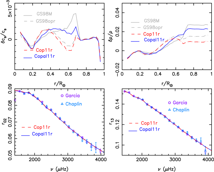
Figure 8: Top panels: relative sound-speed and density differences, in the sense (Sun-Model)/Model, between the Sun and models. The solar sound speed and density are given in Basu et al. (2009). Bottom panels: distributions of observed and predicted ratios $r_{02}$ and $r_{13}$ as a function of frequency. The circles and triangles show the ratios calculated from the frequencies observed by GOLF & VIRGO (García et al., 2011) and BiSON (Chaplin et al., 1999), respectively.

The fluxes of $pp$, $pep$, $hep$, ⁷Be, and ⁸B neutrinos and the total fluxes of ¹³N, ¹⁵O, and ¹⁷F neutrinos calculated from Copal11r are in agreement with those detected by Borexino Collaboration (2018, 2020) at the level of $1\sigma$. The ⁸B neutrino flux of $5.41\times 10^{6}$ cm^-2 s^-1 is also in good agreement with $(5.21\pm 0.27)\times 10^{6}$ cm^-2 s^-1 (Ahmed et al., 2004) but larger than that determined by Bergström et al. (2016) (see Table 2). Copal11r not only is in agreement with updated neutrino fluxes but has better sound-speed and density profiles than GS98M (see Figure 8 or Table 4). It is thus better than GS98M.

The surface heavy-element abundance of Cop11r is also $0.01548$. Cop11r has better sound-speed and density profiles (smaller $\chi^{2}_{c_{s}+\rho}$) than Copal11r (see Figure 8 and Table 4). It also reproduces the observed $r_{02}$ and $r_{13}$, inferred radius $r_{cz}$, and updated neutrino fluxes except the ⁸B neutrino flux. The ⁸B neutrino flux of Cop11r is $5.16\times 10^{6}$ cm^-2 s^-1, which is lower than $5.68^{+0.39}_{-0.41}\times 10^{6}$ cm^-2 s^-1 (Borexino Collaboration, 2018) but in good agreement with that determined by Bergström et al. (2016). The surface helium abundance of $0.2431$ for Cop11r is lower than $0.2485\pm 0.0035$ inferred by Basu & Antia (2004) but consistent with $0.2423\pm 0.0054$ advocated by Asplund et al. (2021). OP significantly improves the sound-speed and density profiles, but leads to the fact that the ⁸B neutrino flux and surface helium abundance are lower than the inferred values. However, if $\Phi(^{8}\rm B)=5.16^{+0.13}_{-0.09}\times 10^{6}$ cm^-2 s^-1 (Bergström et al., 2016) and $Y_{s}=0.2423\pm 0.0054$ (Asplund et al., 2021) are adopted, the $\Phi(^{8}\rm B)$ and $Y_{s}$ of GS98op are more consistent with these values than those of GS98M. In this case, GS98op is the best SSM with high metal abundances rather than GS98M; and Cop11r is better than GS98op.

Models Cop11r and Copal11r have the same input physics except opacity tables. The models constructed with OP opacity tables have better sound-speed and density profiles but lower surface helium abundance and ⁸B neutrino flux than those constructed with OPAL opacity tables. The differences in the sound-speed and density profiles, surface helium abundances, and ⁸B neutrino fluxes caused by the discrepancies in the opacities are marked. The results indicate that a small discrepancy in opacities can obviously affect the solar model.

3.3 Possible Problems in Opacities

In order to understand the effects of the differences in opacities on models, we constructed model Aop12ri with OP opacity tables and Copal11ri with OPAL opacity tables. The OP opacities in the regions of Aop12ri with $T\gtrsim 4.5\times 10^{6}$ K ($r\lesssim 0.45$ $R_{\odot}$) were increased by about $1.5\%$ ($k_{0}\leq 1.015$, see Appendix A) to approximately match OPAL opacities in the same regions. The OPAL opacities for the regions of Copal11ri with $2\times 10^{6}$ K $\lesssim T\lesssim 5\times 10^{6}$ K were increased by about $1-2.3\%$ ($k_{0}\leq 1.023$) to roughly match OP opacities (see Figure 9). The fundamental parameters and neutrino fluxes of these two models are also listed in Tables 1 and 2, respectively.

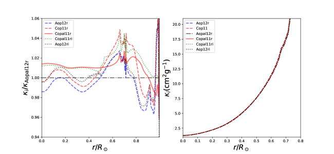
Figure 9: Left panel: comparison of Rosseland mean opacity of different models relative to that of Aopal12r. Right panel: distributions of Rosseland mean opacity of the models as a function of radius.

Aop12ri is in good agreement with helioseismic results and updated neutrino fluxes except the surface helium abundance and ⁸B neutrino flux. The surface helium abundance of Aop12ri is $0.2436$, which is lower than the seismically inferred value of $0.2485\pm 0.035$. Moreover, the ⁸B neutrino flux of Aop12ri is $5.19\times 10^{6}$ cm^-2 s^-1, which is lower than that detected by Borexino Collaboration (2018). But they are higher than those of Aop12r. The increase in OP opacities mainly improves the predictions of surface helium abundance and ⁸B neutrino flux but slightly worsens the sound-speed and density profiles in comparison to those of Aop12r (see Table 4 or Figures 8 and 10). However, the sound-speed and density profiles of Aop12ri are still better than those of GS98M.

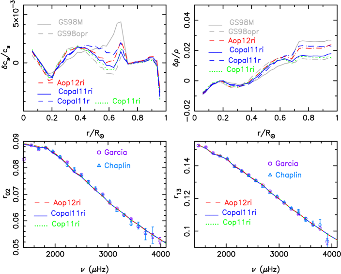
Figure 10: Top panels: relative sound-speed and density differences, in the sense (Sun-Model)/Model, between the Sun and models. The solar sound speed and density are given in Basu et al. (2009). Bottom panels: distributions of observed and predicted ratios $r_{02}$ and $r_{13}$ as a function of frequency. The circles and triangles show the ratios calculated from the frequencies observed by GOLF & VIRGO (García et al., 2011) and BiSON (Chaplin et al., 1999), respectively.

The increase in OPAL opacities has almost no effect on surface helium abundance and neutrino fluxes (see Table 2) but significantly improves the sound-speed and density profiles (see Figure 10). The relative differences $\delta c_{s}/c_{s}$ and $\delta\rho/\rho$ between Sun and Copal11ri are smaller than $0.00117$ and $0.0178$ near the BCZ, decreased by about $46\%$ and $29\%$ in comparison to those of Copal11r, respectively. Copal11ri reproduces the observed ratios $r_{02}$ and $r_{13}$ (see Figure 10) and the inferred helium abundance and $r_{cz}$ at the level of $1\sigma$. The neutrino fluxes calculated from Copal11ri also agree with those detected by Borexino Collaboration (2018, 2020) at the level of $1\sigma$. Copal11ri is the best rotating model for the heavy-element abundance determined by Caffau et al. (2010). It is better than Copal11r and in good agreement with helioseismic results and updated neutrino fluxes.

The increase in OPAL opacities works well. The changes in OP opacities would have the same effect. In order to test this case, we constructed model Cop11ri. The OP opacities for the regions of Cop11ri with $T\gtrsim 4.5\times 10^{6}$ K were increased by about $1.5\%$ to approximately match OPAL opacities in the same regions. The calculations show that models Cop11ri and Copal11ri have almost the same sound-speed and density profiles (see Figure 10), surface helium and heavy-element abundances (see Table 1), and neutrino fluxes (see Table 2). They also have almost the same $Z_{0}$, $Y_{0}$, and $\alpha_{\rm{MLT}}$. The modified OP and OPAL opacities produce almost the same rotating models. These imply that the differences between Cop11r and Copal11r result from discrepancies in opacities, and that OPAL might underestimate opacities for the regions of the Sun with $2\times 10^{6}$ K $\lesssim T\lesssim 5\times 10^{6}$ K by about $1-2\%$, or that OP might underestimate opacities in the regions of the Sun with $T\gtrsim 4.5\times 10^{6}$ K by around $1.5\%$. The possible underestimate in OP leads to the fact that the models constructed with OP opacity tables have a lower surface helium abundance and ⁸B neutrino flux than those constructed with OPAL opacity tables, while the possible underestimate in OPAL results in the fact that the sound-speed and density profiles of the models constructed with OPAL opacity tables are not as good as those of the models constructed with OP opacity tables.

With the modified opacities, only the models with the metal abundance determined by Lodders (2020) agree with the ⁸B neutrino flux determined by Bergström et al. (2016) and the helium abundance advocated by Asplund et al. (2021), but the models with the metal abundance determined by Caffau et al. (2010) are in agreement with the ⁸B neutrino flux detected by Borexino Collaboration (2018) and the seismically inferred helium abundance. Thus precisely determining ⁸B neutrino flux aids in solving the solar abundance problem.

4 Discussion and Summary

Although GS98M was chosen as the best SSM with high metal abundances, the value of $\Phi(\rm CNO)$ of GS98M is slightly larger than the detected value of $7^{+3}_{-2}\times 10^{8}$ cm^-2 s^-1 (Borexino Collaboration, 2020). That of GS98opr is in agreement with the detected one, but its ⁸B neutrino flux is lower than that updated by Borexino Collaboration (2018). Thus the updated neutrino fluxes do not favour the high-Z models. Moreover, the values of $\Phi(\rm CNO)$ calculated from the models with the heavy-element abundance determined by Asplund et al. (2021) are consistent with the detected value, but the ⁷Be and ⁸B neutrino fluxes predicted by the models are much lower than those determined by Bergström et al. (2016) and ones detected by Borexino Collaboration (2018). Therefore, the updated neutrino fluxes also do not prefer the models with the heavy-element abundance determined by Asplund et al. (2021). For the same input physics, the fluxes of ⁷Be, ⁸B, ¹³N, ¹⁵O, and ¹⁷F neutrinos predicted by models increase with an increase in metallicity. These imply that the updated neutrino fluxes prefer a heavy-element abundance between that determined by GS98 and one advocated by Asplund et al. (2021).

Convection was treated according to the standard mixing-length theory (Böhm-Vitense, 1958) in this work. The treatment of convection is one of the sources of uncertainty in modeling of stars. Different treatments of convection, such as Joyce & Chaboyer (2018), Spada et al. (2018, 2019), and Jermyn et al. (2022), could affect solar models and deserve more detailed study.

There are many $T-\tau$ relations for solar atmosphere (Krishna Swamy, 1966; Ball, 2022). The temperature, $T$ reaches $T_{\mathrm{eff}}$ at $\tau=2/3$ for the Eddington approximation but $\tau=0.312156330$ for the Krishna Swamy (1966) $T-\tau$ relation, i.e. the solar radius R is defined at an outer layer for the Krishna Swamy (1966) $T-\tau$ relation. As a consequence, the Krishna Swamy (1966) $T-\tau$ relation requires a larger $\alpha_{\rm{MLT}}$ to reproduce solar radius than the Eddington approximation (Demarque et al., 2008; Joyce & Chaboyer, 2018; Spada et al., 2018). In order to study the effect of the $T-\tau$ relation on our results, we computed the solar models with the Eddington approximation. The calculations show that the $T-\tau$ relation has hardly any influence on neutrino fluxes, frequency separation ratios, and sound-speed and density profiles in the radiative region, but slightly affects the sound-speed and density profiles in the CZ (lead to a slight increase in $\chi^{2}_{c_{s}+\rho}$). Choosing between the Eddington approximation or Krishna Swamy (1966) $T-\tau$ relation does not change our results.

Rotational mixing can more efficiently inhibit the settling of helium than of heavy-element abundances because the mixing depends on the gradient of elements (Yang, 2019). It can reduce the amount of the surface helium settling by about $33-36\%$ in our models, which is consistent with the result of Proffitt & Michaud (1991), who found that macroscopic turbulent mixing can reduce the amount of the surface helium settling by around $40\%$. It leads to the fact that the surface helium abundances of rotating models are obviously higher than those of non-rotating models. In the enhanced diffusion models, the velocity of diffusion and settling was increased by $36\%$. However, we have no obvious physical justification for the multiplier. In non-rotating models, the enhanced diffusion leaves the surface helium abundance too low. However, rotational mixing completely counteracts the effect of the enhanced diffusion on the surface helium abundance in rotating models. Thus the surface helium abundances of the rotating models with the enhanced diffusion are higher than those of non-rotating models. The effects of rotation and enhanced diffusion bring low-Z models into agreement with helioseismic results (Basu & Antia, 2004; Basu et al., 2009) and updated neutrino fluxes (Borexino Collaboration, 2018, 2020). However, the calculations show that the same effects can not bring high-Z models into agreement with the helioseismic results and the updated neutrino fluxes at the same time.

The effects of rotation and enhanced diffusion were studied by Yang (2019), where the value of multiplier ($f_{0}$) was larger than or equal to $1.5$ and OPAL opacity tables constructed in accordance with AGSS09 mixtures were used. The flux of ⁷Be neutrino and the total fluxes of ¹³N, ¹⁵O, and ¹⁷F neutrinos predicted by the best model of Yang (2019) are larger than those detected by Borexino Collaboration (2018, 2020). The ⁷Be neutrino flux is also higher than that determined by Bergström et al. (2016). Different from the earlier models of Yang (2019), Copal11r and Copal11ri, in which the value of multiplier is $1.36$ and opacity tables are reconstructed in accordance with Caffau et al. (2011) mixtures, are in good agreement with the detected neutrino fluxes at the level of $1\sigma$.

The differences between OPAL and OP opacities are small but can obviously affect the properties of solar models. The ⁸B neutrino fluxes computed from models constructed with OP opacity tables are lower than those calculated from models constructed with OPAL opacity tables, which derives from the fact that OP underestimates opacities for the regions of the Sun with $T\gtrsim 5\times 10^{6}$ K by about $1.5\%$ compared to OPAL, especially in the core. As a consequence, the models constructed with OP opacity tables disagree with the ⁸B neutrino flux detected by Borexino Collaboration (2018) but can agree with that determined by Bergström et al. (2016). Thus precisely determining the ⁸B neutrino flux aid in diagnosing the opacities in the solar core.

Moreover, the sound-speed and density profiles of models constructed with OPAL opacity tables are obviously not as good as those of models constructed with OP opacity tables, which results from the fact that OPAL underestimates opacities for the regions of the Sun with $2\times 10^{6}$ K $\lesssim T\lesssim 5\times 10^{6}$ K by about $1-2\%$ compared to OP. If OPAL opacities in the regions are increased by about $1-2\%$ to approximately match OP opacities for the same regions, the models constructed with the OPAL opacities will produce better sound-speed and density profiles. If OP opacities for the regions of the Sun with $T\gtrsim 5\times 10^{6}$ K are increased by about $1.5\%$, the model constructed with the OP opacities will be almost the same as that constructed with the modified OPAL opacities. These imply that the discrepancies between the sound speed and density of the Sun and those of the models could partly derive from opacity. The small differences between OPAL and OP opacities can obviously affect sound-speed and density profiles, surface helium abundance, and neutrino fluxes of models, which do not depend on mixture patterns. But the effect on neutrino fluxes slightly relies on the value of $Z_{0}$. In order to improve the solar model, the discrepancies between OPAL and OP may deserve more studies.

In this work, by using OP and OPAL opacity tables reconstructed with AAG21 and Caffau’s mixtures, we constructed rotating solar models in which the effects of convection overshoot and enhanced diffusion were included. We obtained a rotating model, Copal11r, that is better than the SSM GS98M and the earlier rotating models of Yang (2016, 2019). The surface heavy-element abundance of Copal11r is $0.01548$, which is consistent with the value of $0.0154$ determined by Caffau et al. (2010) and that inferred by Basu & Antia (2004). The surface helium abundance of $0.2450$ and the radius of the BCZ of $0.714$ $R_{\odot}$ are in agreement with the seismically inferred values at the level of $1\sigma$. The initial helium abundance is $0.2718$, which is consistent with the value of $0.273\pm 0.006$ inferred by Serenelli & Basu (2010). The ratios $r_{02}$ and $r_{13}$ of Copal11r agree with those calculated from observed frequencies. The sound-speed and density profiles of Copal11r are better than those of GS98M. Moreover, the fluxes of $pp$, $pep$, $hep$, ⁷Be, and ⁸B neutrinos and the total fluxes of ¹³N, ¹⁵O, and ¹⁷F neutrinos calculated from Copal11r agree with those detected by Borexino Collaboration (2018, 2020) at the level of $1\sigma$. The fluxes of ⁷Be and ⁸B neutrinos are also consistent with those determined by Bellini et al. (2011) and Ahmed et al. (2004). To recover the seismically inferred depth of the CZ, a convection overshoot of $\delta_{\rm ov}\approx 0.1$ is required in rotating models. Rotation or enhanced diffusion alone can improve sound-speed and density profiles, but the combination of rotation and enhanced diffusion is required to bring the rotating model into agreement with seismically inferred results and detected neutrino fluxes. More details of Copal11r are given in Appendix C.

If the surface helium abundance of $0.2423\pm 0.0054$ advocated by Asplund et al. (2021) and the ⁸B neutrino flux determined by Bergström et al. (2016) are adopted, we can obtain another rotating model, Cop11r, that is better than GS98op. The models constructed with OP opacity tables have obviously better sound-speed and density profiles but lower surface helium abundance and ⁷Be, ⁸B, ¹³N, ¹⁵O, and ¹⁷F neutrino fluxes than those constructed with OPAL opacity tables. The calculations show that OPAL may underestimate opacities for the regions of the Sun with $2\times 10^{6}$ K $\lesssim T\lesssim 5\times 10^{6}$ K by about $1-2\%$, and that OP may underestimate opacities in the regions of the Sun with $T\gtrsim 5\times 10^{6}$ K by around $1.5\%$. If the possible underestimate of OPAL or OP were corrected, the model better than Copal11r or Cop11r would be obtained.

Table 1: Fundamental Parameters of Solar Models Constructed in Accordance with Different Mixtures.

Model	$Y_{0}$	$Z_{0}$	$\alpha_{\rm{MLT}}$	$\delta_{\rm ov}$	$f_{0}$	$\rho_{c}$	$r_{cz}$	$Y_{s}$	$Z_{s}$	$(Z/X)_{s}$	$\Delta Y$	$\Omega_{i}$
Opacity Tables Constructed with GS98 mixtures
GS98M	0.2761	0.01940	2.1223	0	1.0	154.59	0.716	0.2455	0.0174	0.0237	0.0306	0
GS98Mr	0.2735	0.01896	2.0754	0.05	1.0	154.11	0.715	0.2534	0.0170	0.0234	0.0201	10
GS98op	0.2713	0.01894	2.1352	0	1.0	154.25	0.716	0.2414	0.0170	0.0230	0.0299	0
GS98opr	0.2711	0.01890	2.0979	0.05	1.0	154.16	0.714	0.2512	0.0170	0.0232	0.0199	10
Opacity Tables Constructed with AAG21 mixtures
Aop01	0.2583	0.01557	2.0722	0	1.0	151.98	0.725	0.2283	0.0139	0.0184	0.0300	0
Aop02	0.2648	0.01661	2.0954	0	1.0	152.89	0.722	0.2347	0.0149	0.0199	0.0301	0
Aop01r	0.2582	0.01554	2.0383	0.15	1.0	151.86	0.716	0.2389	0.0140	0.0187	0.0193	10
Aop02r	0.2648	0.01659	2.0596	0.15	1.0	152.88	0.713	0.2453	0.0149	0.0202	0.0195	10
Aop12r	0.2675	0.01717	2.1055	0.10	1.36	154.42	0.714	0.2413	0.0149	0.0201	0.0262	10
Aopal12r	0.2690	0.01720	2.0872	0.10	1.36	154.27	0.714	0.2424	0.0149	0.0201	0.0266	10
Aop12ri	0.2702	0.01722	2.0918	0.10	1.36	154.34	0.715	0.2436	0.0149	0.0202	0.0266	10
Opacity Tables Constructed with Caffau mixtures
Cop01	0.2666	0.01719	2.0924	0	1.0	152.87	0.720	0.2365	0.0154	0.0206	0.0301	0
Cop01r	0.2664	0.01714	2.0582	0.12	1.0	152.76	0.714	0.2467	0.0154	0.0209	0.0197	10
Cop11r	0.2695	0.01780	2.1056	0.10	1.36	154.42	0.711	0.2431	0.01548	0.0209	0.0264	10
Cop11ri	0.2717	0.01777	2.0883	0.10	1.36	154.29	0.714	0.2450	0.0154	0.0209	0.0267	10
Copal11r	0.2717	0.01784	2.0817	0.10	1.36	154.25	0.713	0.2450	0.01548	0.0209	0.0267	10
Copal11ri	0.2720	0.01774	2.0865	0.10	1.36	154.46	0.712	0.2453	0.0154	0.0209	0.0267	10

Note. — The central density $\rho_{c}$, CZ radius $r_{cz}$, and initial angular velocity $\Omega_{i}$ are in units of g cm^-3, $R_{\odot}$, and $10^{-6}$ rad s^-1, respectively. The quantity $\Delta Y=Y_{0}-Y_{s}$ is the amount of surface helium settling.

Table 2: Predicted and Measured Solar Neutrino Fluxes.

model	$T_{c}$	$pp$	$pep$	$hep$	7Be	8B	13N	15O	17F
BP04	…	5.94	1.40	7.88	4.86	5.79	5.71	5.03	5.91
SSeM	…	5.92	1.39	….	4.85	4.98	5.77	4.97	3.08
Measured	…	6.06${}^{+0.02a}_{-0.06}$	1.6$\pm$0.3b	…	4.84$\pm$0.24a	5.21$\pm$0.27c	…	…	…
B16d	…	5.97${}^{+0.04}_{-0.03}$	1.448$\pm$0.013	19${}^{+12}_{-9}$	4.80${}^{+0.24}_{-0.22}$	5.16${}^{+0.13}_{-0.09}$	$\leq$13.7	$\leq$2.8	$\leq$85
Borexinoe	…	6.1$\pm$0.5	1.39$\pm$0.19	$<$220	4.99$\pm$0.11	5.68${}^{+0.39}_{-0.41}$	7${}^{+3}_{-2}$
GS98M	15.777	5.95	1.40	9.69	5.09	5.59	5.40	4.77	5.52
GS98Mr	15.733	5.96	1.41	9.73	4.95	5.29	5.08	4.45	5.14
GS98op	15.706	5.98	1.42	9.81	4.92	5.18	4.97	4.35	5.02
GS98opr	15.693	5.97	1.41	9.78	4.86	5.07	4.90	4.28	4.93
Aop01	15.513	6.05	1.45	10.19	4.42	4.12	3.43	2.91	3.32
Aop02	15.604	6.02	1.43	9.79	4.66	4.60	3.97	3.43	3.93
Aop01r	15.498	6.03	1.44	10.15	4.36	4.01	3.37	2.85	3.25
Aop02r	15.598	6.01	1.43	9.99	4.63	4.55	3.94	3.40	3.89
Aop12r	15.680	5.97	1.42	9.84	4.82	4.98	4.45	3.88	4.47
Aopal12r	15.706	5.97	1.42	9.81	4.87	5.09	4.54	3.96	4.57
Aop12ri	15.715	5.96	1.41	9.77	4.91	5.19	4.61	4.04	4.66
Cop01	15.645	6.00	1.42	9.95	4.75	4.82	4.25	3.69	4.24
Cop01r	15.623	5.98	1.42	9.92	4.66	4.65	4.16	3.59	4.12
Cop11r	15.716	5.95	1.41	9.77	4.89	5.16	4.73	4.15	4.79
Cop11ri	15.751	5.94	1.40	9.70	4.99	5.38	4.90	4.32	4.99
Copal11r	15.761	5.95	1.41	9.71	4.99	5.41	4.93	4.34	5.03
Copal11ri	15.764	5.95	1.41	9.72	5.00	5.44	4.92	4.34	5.02

Note. — The table shows the predicted fluxes, in units of $10^{10}(pp)$, $10^{9}(^{7}\mathrm{Be})$, $10^{8}(pep,^{13}\mathrm{N},^{15}\mathrm{O})$, $10^{6}(^{8}\mathrm{B},^{17}\mathrm{F})$, and $10^{3}(hep)$ $\mathrm{cm}^{2}$ $\mathrm{s}^{-1}$. The central temperature $T_{c}$ of models is in unit of $10^{6}$ K. The BP04 is the best model of Bahcall & Pinsonneault (2004) and has the GS98 mixtures. The SSeM is the best seismic model with high metal abundances that can reproduce inferred sound speed (Turck-Chièze & Couvidat, 2011).

Table 3: Physical Configurations of Models.

Model Name	Mixtures	Opacity	Enhanced Diffusion	$Z_{s}$ value	Rotation	Increased Opacity ($k_{0}$)a
GS98M	GS98	OPAL	No	GS98	No	No
GS98Mr	GS98	OPAL	No	GS98	Yes	No
GS98op	GS98	OP	No	GS98	No	No
GS98opr	GS98	OP	No	GS98	Yes	No
Aop01	AAG21b	OP	No	AAG21	No	No
Aop02	AAG21	OP	No	Lodders 2020	No	No
Aop01r	AAG21	OP	No	AAG21	Yes	No
Aop02r	AAG21	OP	No	Lodders 2020	Yes	No
Aop12r	AAG21	OP	Yes	Lodders 2020	Yes	No
Aop12ri	AAG21	OP	Yes	Lodders 2020	Yes	Yes($1\leq k_{0}\leq 1.015$)
Aopal12r	AAG21	OPAL	Yes	Lodders 2020	Yes	No
Cop01	Caffauc	OP	No	Caffau	No	No
Cop01r	Caffau	OP	No	Caffau	Yes	No
Cop11r	Caffau	OP	Yes	Caffau	Yes	No
Cop11ri	Caffau	OP	Yes	Caffau	Yes	Yes($1\leq k_{0}\leq 1.015$)
Copal11r	Caffau	OPAL	Yes	Caffau	Yes	No
Copal11ri	Caffau	OPAL	Yes	Caffau	Yes	Yes($1\leq k_{0}\leq 1.023$)

Note. — ^a See the Appendix A. ^bSee the Table 5 in Appendix A and Asplund et al. (2021). ^cSee the Table 5 and Caffau et al. (2010, 2011).

Table 4: The Values of $\chi^{2}$ of Different Models.

Model	$\chi^{2\ a}_{c_{s}+\rho}$	$\chi^{2\ b}_{d_{02+13}}$	$\chi^{2\ c}_{Borexino-neutrino}$	$\chi^{2\ d}_{\rm helium}$
GS98M	882.4	1.2	0.53	0.7
GS98Mr	799.2	1.4	0.49	2.0
GS98op	578.2	1.8	0.61	4.1
GS98opr	369.6	1.5	0.88	0.6
Aop01	6244.7	19.0	7.08	33.3
Aop02	3144.1	16.2	2.85	15.5
Aop01r	4424.0	9.0	8.43	7.5
Aop02r	1983.0	7.0	3.23	0.8
Aop12r	389.1	1.7	1.11	4.2
Aopal12r	917.4	1.6	0.78	3.0
Aop12ri	524.3	2.0	0.57	2.0
Cop01	2440.7	8.3	1.72	11.8
Cop01r	1402.2	6.5	2.75	0.3
Cop11r	323.7	1.6	0.67	2.4
Cop11ri	369.7	1.8	0.38	1.0
Copal11r	590.6	1.5	0.37	1.0
Copal11ri	342.6	1.6	0.35	0.8

Note. — The function $\chi^{2}$ defined as $\chi^{2}=\frac{1}{N}\sum^{N}_{i=1}\frac{(q_{\rm ob,i}-q_{\rm th,i})^{2}}{\sigma^{2}_{i}}$, where $q_{\rm ob,i}$ and $q_{\rm th,i}$ are the observed/inferred and theoretical values of quantities $q_{\rm i}$, respectively; $\sigma_{i}$ are the errors associated to the corresponding observed/inferred quantities; $N$ is the number of the quantities.

Appendix A Opacity Tables

The low-temperature opacity tables with the mixtures listed in Table 5 were downloaded from https://www.wichita.edu/academics/fairmount_college_of_liberal_arts_and_sciences/physics/Research/opacity.php. The OPAL and OP opacity tables with the same mixtures were computed from https://opalopacity.llnl.gov/type1inp.html and http://op-opacity.obspm.fr/opacity/, respectively. The OP opacities did not consider the contributions of P, Cl, K, and Ti compared to OPAL opacities. The contributions of the missing elements (P, Cl, K, and Ti) were automatically transferred to other elements (see the note of the website of OP). The opacity tables, used in this work, are also available at the author’s github repository at https://github.com/yangwuming/SUN.

The low-temperature opacity tables were used in the low-temperature region with $\lg T<4.0$, and OPAL or OP tables were used in the high-temperature region with $\lg T>4.1$. In the region with $4.0\leq\lg T\leq 4.1$, the opacity was linearly interpolated between the high-temperature and low-temperature opacities. Moreover, we corrected the wrong CALL YALO2D in the subroutine YALO3D2 of YREC, which mainly affects the value of mixing-length parameter $\alpha_{\rm{MLT}}$ (lead to a small decrease in $\alpha_{\rm{MLT}}$). For models Aop12ri, Copal11ri, and Cop11ri, we applied a straight multiplier $k_{0}$ to opacity $\kappa$ to enhance the opacity in a given region (see Section 3.3).

Table 5: Fractional Abundances of Heavy Elements Used to Construct Opacity Tables.

Element	Number fraction	Number fraction
	(Caffau’s mixtures)	(AAG21 mixtures)
C	0.260408	0.266509
N	0.059656	0.062476
O	0.473865	0.452597
Ne	0.096751	0.106099
Na	0.001681	0.001534
Mg	0.029899	0.032788
Al	0.002487	0.002487
Si	0.029218	0.029903
P	0.000237	0.000238
S	0.011632	0.012182
Cl	0.000150	0.000189
Ar	0.002727	0.002217
K	0.000106	0.000109
Ca	0.001760	0.001844
Ti	0.000072	0.000086
Cr	0.000385	0.000385
Mn	0.000266	0.000243
Fe	0.027268	0.026651
Ni	0.001431	0.001465

Note. — The number fraction of Caffau’s mixtures were listed by Ferguson in the WSU low temperature opacities, while those of AAG21 mixtures were calculated by using the data in Table 2 of Asplund et al. (2021).

Appendix B Nuclear reactions

The nuclear reaction rates in conjunction with the corresponding energy release of three alternative $pp$ branches ($pp1,pp2,pp3$), CNO cycle, and helium burning are calculated in YREC. The sequence of the reactions is explicitly listed in Demarque et al. (2008). The standard reaction rates implemented are identical to the rates published in Bahcall (1989). The calculated energy generation and neutrino fluxes are dependent on Q-values and nuclear cross-section factors $S_{0}$, respectively. The default Q-values are taken from the Table 21 of Bahcall & Ulrich (1988) and not changed. The default values of nuclear cross-section factors $S_{0}$ are taken from the Tables 3.2 and 3.4 of Bahcall (1989). Compared with the default and those adopted by Bahcall & Pinsonneault (1992), we adopted different $S_{0}(hep)$ and $S_{0}(^{7}\rm{Be}+p)$, which are shown in Table 6. The value of $0.0202$ keV barns of $S_{0}(^{7}\rm{Be}+p)$ (Schramm & Shi, 1994) is in agreement with $0.0205\pm 0.0007$ keV barns of Baby et al. (2003) and $0.0208\pm 0.0007$ keV barns of Adelberger et al. (2011). Moreover, if $S_{0}(hep)=15.3\times 10^{-20}$ keV barns (Wolfs et al., 1989) is adopted, the value of $hep$ flux of model Copal11r is $14.4\times 10^{3}$ cm² s^-1, which is in better agreement with that determined by Bergström et al. (2016). The changes in $S_{0}(hep)$ and $S_{0}(^{7}\rm{Be}+p)$ affect, respectively, only the $hep$ and ⁸B fluxes (Bahcall & Pinsonneault, 2004). All models were computed by using the same Q-values and $S_{0}$.

Table 6: Some of Nuclear Cross-section Factors $S_{0}$ (keV barns).

Reaction	Defaulta	BP92	BP04	This work
1H($p$, e${}^{+}\nu_{e}$ ) 2H	$4.07\times 10^{-22}$	$4.00^{+0.06}_{-0.04}\times 10^{-22}$	$3.94(1\pm 0.004)\times 10^{-22}$	$4.00\times 10^{-22}$
1H($p+e^{-}$, $\nu_{e}$) 2H	Eq. (3.17)a	Eq. (3.17)a	Eq. (3.17)a	Eq. (3.17)a
3He(3He, $2p$) 4He	$5.15\times 10^{3}$	$5.00(1\pm 0.06)\times 10^{3}$	$5.4\times 10^{3}$	$5.00\times 10^{3}$
3He(4He, $\gamma$) 7Be	0.54	$0.533(1\pm 0.032)$	0.533	0.533
7Be($e^{-}$, $\nu_{e}$) 7Li	Eq. (3.18)a	Eq. (3.18)a	Eq. (26)b	Eq. (3.18)a
7Be($p$, $\gamma$) 8B	0.0243	$0.0224(1\pm 0.093)$	0.0206$\pm 0.0008^{c}$	0.0202d
3He($p$, e${}^{+}\nu_{e}$ )4He	$8\times 10^{-20}$	$1.30\times 10^{-20}$	$(8.6\pm 1.3)\times 10^{-20}$	$2.30\times 4.5^{e}\times 10^{-20}$

Note. — ^aBahcall (1989). ^bThe equation of Adelberger et al. (1998). ${}^{c}S_{20\ \rm{keV}}(^{7}\rm{Be}+p)$ given by Junghans et al. (2003). ^dThe value given by Schramm & Shi (1994). ^eThe value of $S_{0}(hep)$ given by Schiavilla et al. (1994) is $2.30\times 10^{-20}$, which should be multiplied by a factor of $4.5$ (Marcucci et al., 2000).

Appendix C Numerical Solar Model and Data Availability

Table 7 presents a basic numerical description of model Copal11r. All models and data used in this work are availabe at the author’s github repository at https://github.com/yangwuming/SUN. In the old YREC, opacity was calculated by linearly interpolating between the opacity of a given $Z_{1}$ and that of another given $Z_{2}$ for heavy-element diffusion. We modified the code to linearly interpolate between a series of $Z$ values (with $\delta Z=0.001$) for the heavy-element diffusion. The amended YREC package, including pulsation code, are available from the author at yangwuming@bnu.edu.cn.

Table 7: Numerical Description of Model Copal11r.

M/M⊙	r/R⊙	L/L⊙	T (K)	$\rho$ (g cm-3)	p (dyn cm-2)	$\kappa$ (cm2 g-1)	X	Y	Z	$\Omega$ (10-6 rad s-1)
0.000001	0.00190	0.00001	1.576e+07	1.542e+02	2.368e+17	1.2914e+00	0.3364	0.6444	0.0192	1.50e-05
0.000002	0.00263	0.00002	1.576e+07	1.542e+02	2.367e+17	1.2916e+00	0.3365	0.6443	0.0192	1.50e-05
0.000003	0.00310	0.00003	1.576e+07	1.541e+02	2.367e+17	1.2917e+00	0.3366	0.6442	0.0192	1.50e-05
0.000005	0.00365	0.00005	1.576e+07	1.541e+02	2.366e+17	1.2918e+00	0.3367	0.6441	0.0192	1.50e-05
0.000009	0.00430	0.00008	1.576e+07	1.540e+02	2.366e+17	1.2920e+00	0.3369	0.6439	0.0192	1.50e-05
0.000014	0.00507	0.00013	1.575e+07	1.539e+02	2.364e+17	1.2922e+00	0.3371	0.6437	0.0192	1.50e-05
0.000023	0.00597	0.00021	1.575e+07	1.538e+02	2.363e+17	1.2926e+00	0.3375	0.6434	0.0192	1.50e-05
0.000038	0.00704	0.00034	1.574e+07	1.537e+02	2.361e+17	1.2931e+00	0.3379	0.6430	0.0191	1.50e-05
0.000062	0.00829	0.00055	1.574e+07	1.534e+02	2.357e+17	1.2938e+00	0.3385	0.6424	0.0191	1.50e-05
0.000102	0.00977	0.00089	1.573e+07	1.531e+02	2.353e+17	1.2947e+00	0.3393	0.6415	0.0191	1.50e-05
0.000166	0.01152	0.00146	1.571e+07	1.527e+02	2.347e+17	1.2960e+00	0.3405	0.6403	0.0191	1.50e-05
0.000272	0.01358	0.00238	1.570e+07	1.521e+02	2.339e+17	1.2979e+00	0.3421	0.6387	0.0191	1.50e-05
0.000444	0.01601	0.00387	1.567e+07	1.512e+02	2.328e+17	1.3004e+00	0.3444	0.6365	0.0191	1.50e-05
0.000726	0.01889	0.00629	1.564e+07	1.501e+02	2.312e+17	1.3039e+00	0.3475	0.6334	0.0191	1.49e-05
0.001187	0.02230	0.01022	1.559e+07	1.485e+02	2.291e+17	1.3087e+00	0.3517	0.6292	0.0191	1.49e-05
0.001939	0.02634	0.01655	1.552e+07	1.463e+02	2.261e+17	1.3149e+00	0.3576	0.6233	0.0191	1.48e-05
0.003168	0.03116	0.02669	1.543e+07	1.434e+02	2.221e+17	1.3236e+00	0.3656	0.6153	0.0191	1.48e-05
0.005179	0.03691	0.04284	1.530e+07	1.394e+02	2.166e+17	1.3357e+00	0.3766	0.6044	0.0191	1.47e-05
0.008465	0.04382	0.06827	1.512e+07	1.342e+02	2.092e+17	1.3526e+00	0.3914	0.5895	0.0190	1.45e-05
0.013830	0.05217	0.10770	1.488e+07	1.274e+02	1.993e+17	1.3763e+00	0.4114	0.5696	0.0190	1.43e-05
0.022608	0.06237	0.16760	1.455e+07	1.187e+02	1.863e+17	1.4098e+00	0.4378	0.5433	0.0189	1.41e-05
0.036949	0.07497	0.25560	1.410e+07	1.079e+02	1.694e+17	1.4577e+00	0.4720	0.5092	0.0188	1.37e-05
0.056968	0.08871	0.36217	1.358e+07	9.657e+01	1.509e+17	1.5169e+00	0.5091	0.4722	0.0187	1.33e-05
0.080715	0.10213	0.46885	1.304e+07	8.624e+01	1.333e+17	1.5799e+00	0.5433	0.4380	0.0186	1.30e-05
0.109607	0.11617	0.57552	1.248e+07	7.636e+01	1.161e+17	1.6526e+00	0.5758	0.4057	0.0185	1.26e-05
0.146362	0.13193	0.68219	1.185e+07	6.642e+01	9.836e+16	1.7429e+00	0.6072	0.3744	0.0184	1.22e-05
0.196727	0.15132	0.78841	1.110e+07	5.573e+01	7.918e+16	1.8647e+00	0.6383	0.3434	0.0183	1.18e-05
0.254970	0.17201	0.87065	1.033e+07	4.595e+01	6.194e+16	2.0069e+00	0.6631	0.3188	0.0182	1.14e-05
0.312918	0.19172	0.92300	9.650e+06	3.798e+01	4.845e+16	2.1549e+00	0.6810	0.3010	0.0181	1.04e-05
0.369383	0.21066	0.95531	9.044e+06	3.149e+01	3.790e+16	2.3107e+00	0.6909	0.2911	0.0180	9.57e-06
0.423543	0.22902	0.97493	8.501e+06	2.610e+01	2.965e+16	2.4761e+00	0.6975	0.2846	0.0179	9.20e-06
0.474881	0.24694	0.98679	8.011e+06	2.160e+01	2.319e+16	2.6534e+00	0.7022	0.2800	0.0179	8.80e-06
0.523093	0.26456	0.99366	7.567e+06	1.786e+01	1.814e+16	2.8464e+00	0.7054	0.2768	0.0178	8.40e-06
0.568053	0.28198	0.99705	7.162e+06	1.474e+01	1.419e+16	3.0574e+00	0.7078	0.2745	0.0177	8.03e-06
0.609743	0.29929	0.99852	6.789e+06	1.215e+01	1.110e+16	3.2874e+00	0.7098	0.2725	0.0177	7.66e-06
0.648210	0.31657	0.99923	6.446e+06	1.001e+01	8.682e+15	3.5379e+00	0.7115	0.2709	0.0177	7.31e-06
0.683576	0.33387	0.99960	6.126e+06	8.229e+00	6.792e+15	3.8109e+00	0.7129	0.2695	0.0176	6.96e-06
0.715985	0.35125	0.99980	5.829e+06	6.762e+00	5.312e+15	4.1078e+00	0.7141	0.2683	0.0176	6.64e-06
0.745591	0.36875	0.99991	5.550e+06	5.552e+00	4.156e+15	4.4296e+00	0.7151	0.2673	0.0176	6.32e-06
0.772576	0.38642	0.99997	5.287e+06	4.556e+00	3.251e+15	4.7782e+00	0.7161	0.2664	0.0175	6.02e-06
0.797116	0.40428	1.00000	5.040e+06	3.737e+00	2.543e+15	5.1556e+00	0.7169	0.2656	0.0175	5.74e-06
0.819381	0.42237	1.00001	4.806e+06	3.064e+00	1.989e+15	5.5644e+00	0.7177	0.2648	0.0175	5.46e-06
0.839548	0.44069	1.00001	4.584e+06	2.511e+00	1.556e+15	6.0050e+00	0.7186	0.2640	0.0174	5.21e-06
0.857782	0.45929	1.00001	4.373e+06	2.058e+00	1.217e+15	6.4815e+00	0.7194	0.2632	0.0174	4.96e-06
0.874233	0.47816	1.00000	4.172e+06	1.686e+00	9.520e+14	7.0002e+00	0.7203	0.2624	0.0174	4.73e-06
0.889056	0.49732	1.00000	3.980e+06	1.382e+00	7.447e+14	7.5656e+00	0.7212	0.2614	0.0174	4.51e-06
0.902387	0.51678	0.99999	3.795e+06	1.132e+00	5.825e+14	8.1805e+00	0.7223	0.2604	0.0173	4.30e-06
0.914354	0.53654	0.99998	3.618e+06	9.283e-01	4.557e+14	8.8490e+00	0.7234	0.2593	0.0173	4.11e-06
0.925080	0.55659	0.99998	3.446e+06	7.614e-01	3.564e+14	9.5772e+00	0.7247	0.2580	0.0173	3.92e-06
0.934675	0.57691	0.99997	3.280e+06	6.251e-01	2.788e+14	1.0375e+01	0.7262	0.2565	0.0173	3.75e-06
0.943239	0.59749	0.99997	3.118e+06	5.137e-01	2.181e+14	1.1257e+01	0.7278	0.2549	0.0173	3.58e-06
0.950869	0.61828	0.99996	2.958e+06	4.230e-01	1.706e+14	1.2250e+01	0.7296	0.2531	0.0173	3.42e-06
0.957649	0.63923	0.99996	2.799e+06	3.491e-01	1.334e+14	1.3427e+01	0.7316	0.2510	0.0174	3.28e-06
0.963657	0.66025	0.99997	2.637e+06	2.894e-01	1.044e+14	1.5065e+01	0.7338	0.2485	0.0177	3.14e-06
0.968963	0.68119	0.99997	2.467e+06	2.417e-01	8.165e+13	1.6387e+01	0.7360	0.2467	0.0173	3.02e-06
0.973526	0.70160	0.99998	2.295e+06	2.041e-01	6.424e+13	1.7759e+01	0.7382	0.2454	0.0164	2.92e-06
0.976002	0.71333	1.00022	2.185e+06	1.854e-01	5.560e+13	1.8426e+01	0.7396	0.2450	0.0155	2.87e-06
0.977337	0.72008	1.00037	2.114e+06	1.764e-01	5.118e+13	1.9703e+01	0.7396	0.2450	0.0155	2.87e-06
0.980936	0.73943	1.00030	1.918e+06	1.522e-01	4.004e+13	2.3806e+01	0.7396	0.2450	0.0155	2.87e-06
0.984045	0.75784	1.00024	1.741e+06	1.313e-01	3.132e+13	2.8373e+01	0.7396	0.2450	0.0155	2.87e-06
0.986711	0.77528	1.00019	1.579e+06	1.133e-01	2.450e+13	3.3468e+01	0.7396	0.2450	0.0155	2.87e-06
0.988982	0.79177	1.00016	1.433e+06	9.775e-02	1.916e+13	3.9246e+01	0.7396	0.2450	0.0155	2.87e-06
0.990904	0.80729	1.00013	1.300e+06	8.435e-02	1.499e+13	4.5830e+01	0.7396	0.2450	0.0155	2.87e-06
0.992521	0.82188	1.00011	1.180e+06	7.278e-02	1.173e+13	5.3219e+01	0.7396	0.2450	0.0155	2.87e-06
0.993874	0.83555	1.00009	1.070e+06	6.280e-02	9.173e+12	6.1516e+01	0.7396	0.2450	0.0155	2.87e-06
0.995001	0.84832	1.00008	9.710e+05	5.419e-02	7.175e+12	7.0972e+01	0.7396	0.2450	0.0155	2.87e-06
0.995933	0.86022	1.00007	8.811e+05	4.677e-02	5.613e+12	8.2430e+01	0.7396	0.2450	0.0155	2.87e-06
0.996702	0.87130	1.00006	7.995e+05	4.036e-02	4.390e+12	9.6834e+01	0.7396	0.2450	0.0155	2.87e-06
0.997334	0.88158	1.00006	7.254e+05	3.483e-02	3.434e+12	1.1441e+02	0.7396	0.2450	0.0155	2.87e-06
0.997850	0.89110	1.00005	6.583e+05	3.006e-02	2.686e+12	1.3527e+02	0.7396	0.2450	0.0155	2.87e-06
0.998271	0.89991	1.00005	5.975e+05	2.594e-02	2.101e+12	1.5967e+02	0.7396	0.2450	0.0155	2.87e-06
0.998613	0.90804	1.00005	5.423e+05	2.239e-02	1.644e+12	1.8885e+02	0.7396	0.2450	0.0155	2.87e-06
0.998889	0.91554	1.00005	4.923e+05	1.932e-02	1.286e+12	2.2482e+02	0.7396	0.2450	0.0155	2.87e-06
0.999113	0.92244	1.00005	4.469e+05	1.668e-02	1.006e+12	2.7065e+02	0.7396	0.2450	0.0155	2.87e-06
0.999292	0.92878	1.00005	4.058e+05	1.439e-02	7.867e+11	3.3250e+02	0.7396	0.2450	0.0155	2.87e-06
0.999436	0.93461	1.00005	3.685e+05	1.242e-02	6.154e+11	4.1670e+02	0.7396	0.2450	0.0155	2.87e-06
0.999552	0.93995	1.00004	3.348e+05	1.072e-02	4.814e+11	5.3263e+02	0.7396	0.2450	0.0155	2.87e-06
0.999644	0.94484	1.00004	3.042e+05	9.247e-03	3.765e+11	6.9405e+02	0.7396	0.2450	0.0155	2.87e-06
0.999718	0.94933	1.00004	2.765e+05	7.979e-03	2.946e+11	9.2024e+02	0.7396	0.2450	0.0155	2.87e-06
0.999777	0.95343	1.00004	2.514e+05	6.883e-03	2.304e+11	1.2436e+03	0.7396	0.2450	0.0155	2.87e-06
0.999823	0.95718	1.00004	2.288e+05	5.936e-03	1.802e+11	1.7082e+03	0.7396	0.2450	0.0155	2.87e-06
0.999860	0.96060	1.00004	2.083e+05	5.118e-03	1.410e+11	2.3811e+03	0.7396	0.2450	0.0155	2.87e-06
0.999890	0.96373	1.00004	1.898e+05	4.411e-03	1.103e+11	3.3552e+03	0.7396	0.2450	0.0155	2.87e-06
0.999913	0.96659	1.00004	1.731e+05	3.798e-03	8.626e+10	4.7501e+03	0.7396	0.2450	0.0155	2.87e-06
0.999931	0.96921	1.00004	1.581e+05	3.269e-03	6.748e+10	6.6841e+03	0.7396	0.2450	0.0155	2.87e-06
0.999946	0.97159	1.00004	1.447e+05	2.810e-03	5.278e+10	9.2032e+03	0.7396	0.2450	0.0155	2.87e-06
0.999957	0.97378	1.00004	1.326e+05	2.412e-03	4.129e+10	1.2213e+04	0.7396	0.2450	0.0155	2.87e-06
0.999967	0.97578	1.00004	1.217e+05	2.068e-03	3.230e+10	1.5468e+04	0.7396	0.2450	0.0155	2.87e-06
0.999974	0.97761	1.00004	1.118e+05	1.772e-03	2.526e+10	1.8710e+04	0.7396	0.2450	0.0155	2.87e-06
0.999979	0.97930	1.00004	1.028e+05	1.516e-03	1.976e+10	2.1823e+04	0.7396	0.2450	0.0155	2.87e-06
0.999984	0.98084	1.00004	9.461e+04	1.298e-03	1.546e+10	2.4907e+04	0.7396	0.2450	0.0155	2.87e-06
0.999987	0.98225	1.00004	8.699e+04	1.111e-03	1.209e+10	2.8321e+04	0.7396	0.2450	0.0155	2.87e-06
0.999990	0.98355	1.00004	7.994e+04	9.521e-04	9.458e+09	3.2562e+04	0.7396	0.2450	0.0155	2.87e-06
0.999994	0.98581	1.00004	6.744e+04	7.004e-04	5.788e+09	4.5889e+04	0.7396	0.2450	0.0155	2.87e-06
0.999996	0.98771	1.00004	5.714e+04	5.143e-04	3.541e+09	6.9908e+04	0.7396	0.2450	0.0155	2.87e-06
0.999998	0.98929	1.00004	4.894e+04	3.749e-04	2.167e+09	1.0278e+05	0.7396	0.2450	0.0155	2.87e-06
0.999999	0.99064	1.00004	4.252e+04	2.701e-04	1.326e+09	1.2664e+05	0.7396	0.2450	0.0155	2.87e-06
0.999999	0.99179	1.00004	3.746e+04	1.923e-04	8.113e+08	1.2530e+05	0.7396	0.2450	0.0155	2.87e-06
0.999999	0.99231	1.00004	3.531e+04	1.616e-04	6.346e+08	1.1637e+05	0.7396	0.2450	0.0155	2.87e-06
0.999999	0.99279	1.00004	3.337e+04	1.355e-04	4.964e+08	1.0456e+05	0.7396	0.2450	0.0155	2.87e-06
1.000000	0.99354	1.00004	3.044e+04	9.966e-05	3.255e+08	8.2105e+04	0.7396	0.2450	0.0155	2.87e-06
1.000000	0.99444	1.00004	2.716e+04	6.534e-05	1.845e+08	5.6764e+04	0.7396	0.2450	0.0155	2.87e-06
1.000000	0.99594	1.00004	2.214e+04	2.646e-05	5.699e+07	2.3956e+04	0.7396	0.2450	0.0155	2.87e-06
1.000000	0.99786	1.00004	1.643e+04	4.852e-06	6.879e+06	4.6756e+03	0.7396	0.2450	0.0155	2.87e-06
1.000000	0.99837	1.00004	1.495e+04	2.667e-06	3.292e+06	2.5776e+03	0.7396	0.2450	0.0155	2.87e-06
1.000000	0.99881	1.00004	1.360e+04	1.469e-06	1.576e+06	1.3462e+03	0.7396	0.2450	0.0155	2.87e-06
1.000000	0.99919	1.00004	1.230e+04	8.173e-07	7.542e+05	6.2276e+02	0.7396	0.2450	0.0155	2.87e-06
1.000000	0.99952	1.00004	1.090e+04	4.663e-07	3.610e+05	2.0916e+02	0.7396	0.2450	0.0155	2.87e-06
1.000000	0.99979	1.00004	8.935e+03	2.874e-07	1.728e+05	2.7659e+01	0.7396	0.2450	0.0155	2.87e-06
1.000000	0.99998	1.00004	6.028e+03	2.073e-07	8.270e+04	5.0052e-01	0.7396	0.2450	0.0155	2.87e-06
1.000000	1.00002	1.00004	5.777e+03	1.719e-07	6.569e+04	3.1819e-01	0.7396	0.2450	0.0155	2.87e-06

References

- Adelberger et al. (1998) Adelberger, E. G., et al. 1998, Rev. Mod. Phys., 70, 1265
- Adelberger et al. (2011) Adelberger E. G., et al. 2011, RMP, 83, 195
- Ahmed et al. (2004) Ahmed, S. N., Anthony, A. E., Beier, E. W. et al. 2004, PhRvL, 92, 1301
- Amarsi et al. (2021) Amarsi, A. M., Grevesse, N., Asplund, M., Collet, R. 2021, A&A, 656, 113
- Antia & Basu (2006) Antia, H. M., & Basu, S. 2006, ApJ, 644, 1292
- Asplund et al. (2021) Asplund, M., Amarsi, A. M., Grevesse, N. 2021, A&A 653, A141
- Asplund et al. (2004) Asplund, M., Grevesesse N., Sauval, A. J., Allende Prieto, C., & Kiselman, D. 2004, A&A, 417, 751
- Asplund et al. (2005) Asplund, M., Grevesesse, N., Sauval, A. J., Allende Prieto, C., & Blomme, R. 2005, A&A, 431, 693
- Asplund et al. (2009) Asplund, M., Grevesse, N., Sauval, A., & Scott, P. 2009, ARA&A, 47, 481 (AGSS09)
- Baby et al. (2003) Baby, L. T., et al. 2003a, Phys. Rev. Lett., 90, 022501
- Badnell et al. (2005) Badnell, N. R., Bautista, M. A., Butler, K., Delahaye, F., Mendoza, C., Palmeri, P., Zeippen, C. J., Seaton, M. J. 2005, MNRAS, 360, 458
- Bahcall (1989) Bahcall, J. N. , 1989, Neutrino Astrophysics (Cambridge University, Cambridge, England).
- Bahcall et al. (2001) Bahcall, J. N., Pinsonneault, M. H., & Basu, S, 2001, ApJ, 555, 990
- Bahcall & Pinsonneault (1992) Bahcall, J. N., & Pinsonneault, M. H. 1992, Rev. Mod. Phys., 64, 885 (BP92)
- Bahcall et al. (1995) Bahcall J. N., Pinsonneault M. H., & Wasserburg G. J. 1995, Rev. Mod. Phys., 67, 781
- Bahcall et al. (2005) Bahcall, J. N., Basu, S., Pinsonneault, M. H., & Serenelli, A. M. 2005, ApJ, 618, 1049