Scaling limit of the disordered
generalized Poland–Scheraga model for DNA denaturation

Abstract.

The Poland–Scheraga model, introduced in the 1970’s, is a reference model to describe the denaturation transition of DNA. More recently, it has been generalized in order to allow for asymmetry in the strands lengths and in the formation of loops: the mathematical representation is based on a bivariate renewal process, that describes the pairs of bases that bond together. In this paper, we consider a disordered version of the model, in which the two strands interact via a potential $\beta V(\widehat{\omega}_{i},\bar{\omega}_{j})+h$ when the $i$-th monomer of the first strand and the $j$-th monomer of the second strand meet. Here, $h\in\mathbb{R}$ is a homogeneous pinning parameter, $(\widehat{\omega}_{i})_{i\geq 1}$ and $(\bar{\omega}_{j})_{j\geq 1}$ are two sequences of i.i.d. random variables attached to each DNA strand, $V(\cdot,\cdot)$ is an interaction function and $\beta>0$ is the disorder intensity. Our main result finds some condition on the underlying bivariate renewal so that, if one takes $\beta,h\downarrow 0$ at some appropriate (explicit) rate as the length of the strands go to infinity, the partition function of the model admits a non-trivial, i.e. disordered, scaling limit. This is known as an intermediate disorder regime and is linked to the question of disorder relevance for the denaturation transition. Interestingly, and unlike any other model of our knowledge, the rate at which one has to take $\beta\downarrow 0$ depends on the interaction function $V(\cdot,\cdot)$ and on the distribution of $(\widehat{\omega}_{i})_{i\geq 1}$, $(\bar{\omega}_{j})_{j\geq 1}$. On the other hand, the intermediate disorder limit of the partition function, when it exists, is universal: it is expressed as a chaos expansion of iterated integrals against a Gaussian process ${\mathcal{M}}$, which arises as the scaling limit of the field $(e^{\beta V(\widehat{\omega}_{i},\bar{\omega}_{j})})_{i,j\geq 0}$ and exhibits strong correlations on lines and columns.

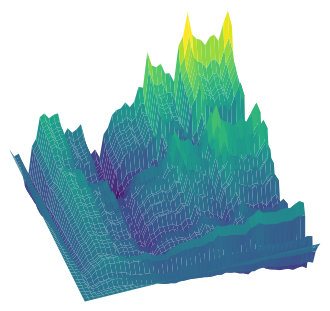
Figure 1. A realization of the (non-isotropic) Gaussian field ${\mathcal{M}}$ appearing in the disordered scaling limit of the generalized Poland–Scheraga model. The field $(V(\widehat{\omega}_{i},\bar{\omega}_{j}))_{i,j\geq 1}$ presents correlations along rows and columns: these correlations appear in the limiting process ${\mathcal{M}}$ and can be observed in the figure above.

1. Introduction

1.1. The Poland–Scheraga model and the question of disorder relevance

The Poland–Scheraga (PS) model [61] has been introduced in the 1970’s in order to describe the denaturation transition of DNA. Since then, it has been widely studied in the bio-physics and mathematical literature, both from a theoretical perspective, see [38, 42, 43], and an experimental one, see e.g. [20, 21]. The model is based on a renewal process that describes the pairs of bases that bind together and it can naturally embed the inhomogeneous character of the interactions between the bases (see Figure 2(a)). More generally, the model is known as the pinning model, which is also used to describe the behavior of one-dimensional interfaces (or polymers) interacting with a defect line. The inhomogeneity of the interactions along the DNA strands is usually modeled thanks to a sequence of random variables, often dubbed as disorder, that represent the different values of the binding potentials along the polymer; in the context of pinning models, this reduces to considering an inhomogeneous (disordered) defect line.

One remarkable feature of the pinning model is that its homogeneous version, that is when the binding potentials are all equals, is solvable. One can show that the model exhibits a depinning (or denaturation) transition and one can identify the critical temperature and the behavior of the free energy when approaching the critical temperature, see [42, Ch. 4].

Disorder relevance

A natural question is then to know whether disorder changes the characteristics of the phase transition: in other words, can we determine if (and how) the critical temperature and the critical behavior of the free energy is affected by the presence of inhomogeneities in the binding interactions? This is the general question of disorder relevance for physical systems: if an arbitrarily small amount of disorder changes the characteristics of the phase transition, then disorder is called relevant; otherwise disorder is called irrelevant. In a celebrated paper, the physicist Harris [50] proposed a general criterion, based on the critical behavior of the homogeneous (or pure) system—more specifically on the correlation length critical exponent $\nu$—, to predict whether an i.i.d. disorder is relevant or not: for a $d$-dimensional physical system, disorder should be irrelevant if $\nu>2/d$ and relevant if $\nu<2/d$; the case $\nu=2/d$, called marginal, requires more investigation.

The pinning model has seen an intense activity over the past decades, both in theoretical physics (see e.g. [33, 35, 36, 39, 53, 67] to cite a few) and in rigorous mathematical physics (see e.g. [3, 5, 9, 13, 32, 34, 46, 47, 48, 49, 54, 68, 69]). One reason for that activity comes from the fact that the homogeneous model is exactly solvable and displays a critical exponent $\nu$ that ranges from $1$ to $+\infty$: the disordered pinning model has therefore been an ideal framework to test the validity of Harris’ predictions. The Harris criterion has now been put on rigorous ground by a series of works (see [3, 5, 32, 34, 48, 49, 54, 68, 69]), the marginal case being also completely settled (see [46, 47] and [13]), after some contradictory predictions in the physics literature [35, 39].

Intermediate disorder regime

A recent and complementary approach to the question of disorder relevance has been to consider scaling limits of the model, see [26] for an overview. In this context, disorder relevance can be understood as the possibility of tuning down the intensity of disorder as the system size grows in such a way that disorder is still present in the limit. The idea is therefore to scale the different parameters of the model with the size of the system, in such a way to obtain a non-trivial, i.e. disordered, scaling limit. This is called the intermediate disorder regime, which corresponds to identifying a scaling window for the disorder intensity in which one observes a transition from a “weak disorder” phase to a “strong disorder” phase.

This approach has first been implemented in the context of the directed polymer model in dimension $1+1$, see [2], and has been widened in [27] to other models (including the pinning model); let us also mention [14, 64] for other results in the same spirit. In particular, let us stress that in [27], the conditions for having a non-trivial scaling limit of the model exactly matches that of Harris’ condition for disorder relevance.

The intermediate disorder scaling limit seems to have wide applications for understanding relevant disorder systems. For instance: it makes it possible to extract universal behaviors of quantities of interest such as the critical point shift or the free energy of the model see [30, 57]; it is a way to construct continuum disordered systems that arise as scaling limits of discrete models (and encapsulate their universal features), see [1, 15, 23, 25]. Let us also mention that, in the case of marginally relevant disordered systems, understanding the intermediate disorder scaling limit is much more challenging, see [28]. However, in the context of the directed polymer in dimension $2+1$ it provides a way to make sense of (and study) the ill-defined stochastic heat equation, see the recent paper [29].

Generalization of the Poland–Scheraga model

The Poland–Scheraga model, thanks to its simplicity, plays a central role in the study of DNA denaturation. But some aspects of it are oversimplified and fail to capture important features of the model: in particular, the two DNA strands are assumed to be of equal length, and loops have to be symmetric, ruling out for instance the existence of mismatches (see Figure 2(a)). For these reasons, Garel and Orland [40] (see also [58]) introduced a generalization of the model that overcomes these two limitations: loops are allowed to be asymmetric and the two strands are allowed to be of different lengths (see Figure 2(b)).

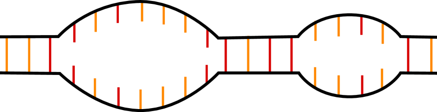
(a) Standard PS model.

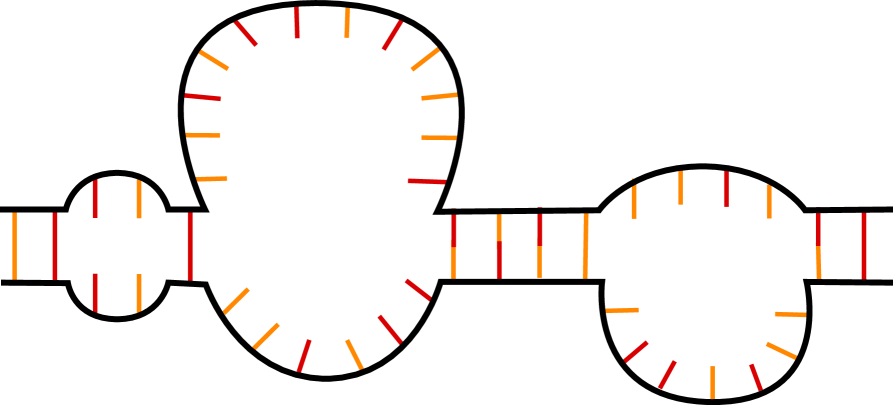
(b) Generalized PS model.

Figure 2. Standard vs. generalized Poland-Scheraga models, with two types of monomers along the strands. The standard PS model is represented on the left: the two strands have the same length and loops are symmetric (there is no mismatch). The configuration is encoded by the sequence of lengths of the successive loops, from left to right (in the example (A): $1,1,8,1,1,1,5,1$). The generalized PS model is represented on the right: the two strands may have different lengths and loops are allowed to be asymmetric. (mismatches occur). A loop is encoded by a pair $(k,\ell)$, with $k$ the length of the ’top’ strand and $\ell$ the length of the ’bottom’ strand in that loop: a configuration is encoded by the sequence of pairs describing the successive loops, from left to right (in the example (B): $(1,1),(3,3),(13,7),(1,1),(1,1),(1,1),(5,8),(1,1)$).

The mathematical formulation of this generalized Poland–Scheraga (gPS) model has been developed by Giacomin and Khatib [45], and is based on a bivariate renewal process, i.e. a renewal process on $\mathbb{N}^{2}$, whose increments describe the successive loops in the DNA (an increment $(k,\ell)$ describes a loop with length $k$ in the first strand and length $\ell$ in the second strand, see Figure 2(b)). In [45], the authors consider only the homogeneous gPS model: somehow surprisingly they find that the model is also solvable, but with a much richer phenomenology than in the PS model. In particular, in addition to the denaturation transition, other phase transitions, called condensation transitions, may occur; this was first observed in [58]. The critical points for the denaturation and condensation transitions can be identified (see [45]). Moreover, the critical behavior of the denaturation transition has been described in [45] and the condensation transitions have been further investigated in [10] (it corresponds to a big-jump transition for the bivariate renewal process).

As far as the disordered version of the gPS model is concerned, this has been investigated in the physics literature, but only at a numerical level, see e.g. [40, 66]. In [11], the authors consider a disordered version of the model, in which a pairing between the $i$-th monomer of the first strand and the $j$-th monomer of the second strand is associated with a disorder variable $\omega_{i,j}$, where $(\omega_{i,j})_{i,j\geq 0}$ are i.i.d. random variables (note that this is not necessarily adapted to the modeling of DNA). In that case, Harris’ predictions for disorder relevance on the denaturation phase transition have been confirmed in [11]: if $\nu$ is the critical exponent for the free energy in the pure model, disorder is irrelevant as soon as $\nu>1$ (here, the dimension of the disorder field is $d=2$). In [56], the author considers the case where the disorder variable $\omega_{i,j}$ associated to the pairing of the $i$-th monomer of the first strand and the $j$-th monomer of the second strand is constructed thanks to two sequences $(\widehat{\omega}_{i})_{i\geq 0},(\bar{\omega}_{j})_{j\geq 0}$ of i.i.d. random variables, representing the inhomogeneities along the two strands. More precisely, [56] takes $\omega_{i,j}=\widehat{\omega}_{i}\bar{\omega}_{j}$ as a natural toy model, for which computations are more explicit. A striking finding of [56] is that, in that case, disorder relevance depends on the distribution of $\widehat{\omega}_{i},\bar{\omega}_{j}$: for “most” distributions, disorder is irrelevant if $\nu>2$ and relevant if $\nu<2$ (the disorder is fundamentally one-dimensional); on the other hand, there are distributions, namely $\frac{1}{2}(\delta_{-x}+\delta_{x})$ for some $x>0$, such that disorder is irrelevant as soon as $\nu>1$ (the disorder is essentially two-dimensional).

Intermediate disorder scaling limit for the gPS model

One of the goal of the present paper is to complement the existing results on the influence of disorder on the denaturation transition for the gPS model. For this purpose, we investigate the intermediate disorder scaling limit of the model, in the spirit of [27, 26]. We extend the results of [56] in several directions:

• We consider a more general disorder variable $\omega_{i,j}$ associated to the pairing of the $i$-th monomer of the first strand and the $j$-th monomer of the second strand: we take $\omega_{i,j}=V(\widehat{\omega}_{i},\bar{\omega}_{j})$ where $(\widehat{\omega}_{i})_{i\geq 0}$, $(\bar{\omega}_{j})_{j\geq 0}$ are sequences of i.i.d. random variables and $V(\cdot,\cdot)$ is any (symmetric) interaction function.

• We identify the correct intermediate disorder scaling and we prove the convergence of the partition function towards a non-trivial limit under that scaling. Remarkably, the scaling depends finely on the distribution of $\omega_{i,j}$, i.e. on the function $V(\cdot,\cdot)$ and on the distribution of $\widehat{\omega}_{i},\bar{\omega}_{j}$.

• The identification of the intermediate disorder scaling allows us to give a sufficient condition for disorder relevance (we determine whether the effective dimension of the disorder is one or two). It also enables us to obtain sharp bounds on the critical point shift, improving some results of [56].

One of the main novelties of the present paper is that, to the best of our knowledge, it is the first instance where the intermediate disorder scaling depends on the distribution of disorder, therefore displaying some non-universality feature. On the other hand, the limit of the partition function under the intermediate disorder scaling is universal, in the sense that it does not depend on the distribution of the disorder $\omega_{i,j}$ or on the fine details of the underlying bivariate renewal.

One major difficulty of the present work is that the disorder field $(\omega_{i,j})_{i,j\geq 0}$ presents some long-range correlations (along lines and columns): as a result, the limit that we obtain is based on a correlated Gaussian field ${\mathcal{M}}$ (see Figure 1 for an illustration) that exhibits the same type of correlations. Note that in the PS model, the question of the influence of long-range correlated disorder on the denaturation transition has been investigated, for instance in [6, 7, 12, 16, 31, 59]. However, to the best of our knowledge, intermediate disorder regimes have so far been considered only in the case of i.i.d. disorder fields (or at least time-independent for models in dimension $1+d$), with the exception of [64]. One can therefore view our result as a new attempt to investigate the influence of a correlated disorder on physical systems.

Some notation

Throughout the article, we write elements of $\mathbb{N}^{2}$, $\mathbb{R}^{2}$ with bold characters, and elements of $\mathbb{N}$, $\mathbb{R}$ with plain characters (in particular we note ${\boldsymbol{0}}:=(0,0)$ and ${\boldsymbol{1}}:=(1,1)$); moreover for $\textbf{{t}}\in\mathbb{R}^{2}$, $\textbf{{t}}^{(a)}$ will denote its projection on its $a$-th coordinate, $a\in\{1,2\}$. When there is no risk of confusion, we may also write more simply $\textbf{{t}}=(t_{1},t_{2})$. We also define orders on $\mathbb{R}^{2}$: for $\textbf{{s}},\textbf{{t}}\in\mathbb{R}^{d}$, write

$$\textbf{{s}}\prec\textbf{{t}}\quad\text{ if }\ s_{1}<t_{1},\,s_{2}<t_{2}\,,\qquad\text{ and }\qquad\textbf{{s}}\preccurlyeq\textbf{{t}}\quad\text{ if }\ s_{1}\leq t_{1},\,s_{2}\leq t_{2}\,.$$

For ${\boldsymbol{0}}\preccurlyeq\textbf{{s}}\preccurlyeq\textbf{{t}}$, let $[\textbf{{s}},\textbf{{t}}]$ denote the rectangle $[s_{1},t_{1}]\times[s_{2},t_{2}]$ (and similarily $[\textbf{{s}},\textbf{{t}}):=[s_{1},t_{1})\times[s_{2},t_{2})$, etc.) and $\llbracket\textbf{{s}},\textbf{{t}}\rrbracket:=[\textbf{{s}},\textbf{{t}}]\cap\mathbb{Z}^{2}$. For $s,t\in\mathbb{R}$, we write $s\wedge t=\min(s,t)$ and $s\vee t=\max(s,t)$; and for $\textbf{{s}},\textbf{{t}}\in\mathbb{R}^{2}$,

$$\textbf{{s}}\wedge\textbf{{t}}\;:=\;(s_{1}\wedge t_{1},s_{2}\wedge t_{2})\qquad\text{and}\qquad\textbf{{s}}\vee\textbf{{t}}\;:=\;(s_{1}\vee t_{1},s_{2}\vee t_{2})\;.$$

For $\textbf{{s}}\in\mathbb{R}^{2}$, let $\lfloor\textbf{{s}}\rfloor:=(\lfloor s_{1}\rfloor,\lfloor s_{2}\rfloor)$. Finally, we will say that $\textbf{{s}},\textbf{{t}}\in\mathbb{R}^{2}$ are aligned if they are on the same line or column, that is if $s_{1}=t_{1}$ or $s_{2}=t_{2}$, and we then write $\textbf{{s}}\leftrightarrow\textbf{{t}}$; otherwise we write $\textbf{{s}}\nleftrightarrow\textbf{{t}}$.

1.2. The generalized Poland-Scheraga model: definition and first properties

Let $\boldsymbol{\tau}=(\boldsymbol{\tau}_{k})_{k\geq 0}$ be a bivariate renewal process, with $\boldsymbol{\tau}_{0}={\boldsymbol{0}}$ and inter-arrival distribution

(1.1) $$\mathbf{P}\big{(}\boldsymbol{\tau}_{1}=(\ell_{1},\ell_{2})\big{)}:=K(\ell_{1}+\ell_{2})=\frac{L(\ell_{1}+\ell_{2})}{(\ell_{1}+\ell_{2})^{2+\alpha}},\qquad\forall\,{\boldsymbol{\ell}}=(\ell_{1},\ell_{2})\in\mathbb{N}^{2}\,,$$

with $\mathbf{P}(|\boldsymbol{\tau}_{1}|<+\infty)=1$. With a slight abuse of notation, we also interpret $\boldsymbol{\tau}$ as a set $\{\boldsymbol{\tau}_{1},\boldsymbol{\tau}_{2},\ldots\}$ (we will always omit $\boldsymbol{\tau}_{0}$).

Let $\widehat{\omega}=(\widehat{\omega}_{i})_{i\geq 1}$ and $\bar{\omega}=(\bar{\omega}_{i})_{i\geq 1}$ be two independent sequences of i.i.d. random variables, whose laws are denoted $\widehat{\mathbb{P}}$ and $\bar{\mathbb{P}}$ respectively. We assume that $\widehat{\mathbb{P}}=\bar{\mathbb{P}}$ and we let $\mathbb{P}:=\widehat{\mathbb{P}}\otimes\bar{\mathbb{P}}$. For $\textbf{{i}}\in\mathbb{N}^{2}$, we denote $\omega_{\textbf{{i}}}=\omega_{i_{1},i_{2}}:=V(\widehat{\omega}_{i_{1}},\bar{\omega}_{i_{2}})$, where $V(\cdot,\cdot)$ is a symmetric function describing the interactions between the monomers; we naturally assume that $V(\cdot,\cdot)$ is not constant. Let us stress that $\omega:=(\omega_{\textbf{{i}}})_{\textbf{{i}}\in\mathbb{N}^{2}}$ is a strongly correlated field. Throughout the paper, we assume that there is some $\beta_{0}>0$ such that

$$\lambda(\beta):=\log\mathbb{E}[e^{\beta\omega_{{\boldsymbol{1}}}}]<+\infty\qquad\text{ for }\beta\in[0,\beta_{0})\,.$$

Example 1.1.

A first, natural example, is to take $V$ in a product form, that is $V(x,y)=f(x)f(y)$ for some function $f$: this is the choice made in [56], with $f(x)=x$. Another natural example would be to take $V(x,y)=g(x+y)$, for some function $g$.

Remark 1.2.

Recalling that the gPS model was introduced to model DNA denaturation, it would also be natural to consider a field $(\omega_{\textbf{{i}}})_{\textbf{{i}}\in\mathbb{N}^{2}}$ defined as a function of a unique sequence $(\widetilde{\omega}_{i})_{i\geq 1}$ of i.i.d. random variables, by $\omega_{\textbf{{i}}}=V(\widetilde{\omega}_{i_{1}},\widetilde{\omega}_{i_{2}})$, with $V$ a symmetric function. Our approach would actually provide results very similar to the one we obtain in the setting described above. We comment in Section 2.5.3 below what is expected when constructing $\omega$ with a unique sequence $\widetilde{\omega}$, but we do not develop that case any further since it becomes more technical and should not bring much different results.

For a fixed realization of $\omega$ (quenched disorder), we define, for $\beta\geq 0$ (the disorder strength) and $h\in\mathbb{R}$ (the pinning potential), the following polymer measures: for any $\textbf{{n}}\in\mathbb{N}^{2}$, representing the respective lengths of the strands, let

(1.2) $$\frac{\mathrm{d}\mathbf{P}_{\textbf{{n}},h}^{\beta,\omega,\mathrm{q}}}{\mathrm{d}\mathbf{P}}(\tau):=\frac{1}{Z_{\textbf{{n}},h}^{\beta,\omega,\mathrm{q}}}\exp\Big{(}\sum_{\textbf{{i}}\in\llbracket{\boldsymbol{1}},\textbf{{n}}\rrbracket}\big{(}\beta\omega_{\textbf{{i}}}-\lambda(\beta)+h\big{)}{\sf 1}_{\{\textbf{{i}}\in\boldsymbol{\tau}\}}\Big{)}{\sf 1}_{\{\textbf{{n}}\in\boldsymbol{\tau}\}},$$

where

(1.3) $$Z_{\textbf{{n}},h}^{\beta,\omega,\mathrm{q}}:=\mathbf{E}\Big{[}\exp\Big{(}\sum_{\textbf{{i}}\in\llbracket{\boldsymbol{1}},\textbf{{n}}\rrbracket}\big{(}\beta\omega_{\textbf{{i}}}-\lambda(\beta)+h\big{)}{\sf 1}_{\{\textbf{{i}}\in\boldsymbol{\tau}\}}\Big{)}{\sf 1}_{\{\textbf{{n}}\in\boldsymbol{\tau}\}}\Big{]}$$

is the partition function of the system. This corresponds to giving a reward (or penalty if it is negative) $\beta\omega_{\textbf{{i}}}+h$ if $\textbf{{i}}=(i_{1},i_{2})\in\boldsymbol{\tau}$, that is if monomer $i_{1}$ of the first strand is paired with monomer $i_{2}$ of the second strand. The term $-\lambda(\beta)$ is only present for renormalization purposes, and even though $Z_{\textbf{{n}},h}^{\beta,\omega,\mathrm{q}}$ depends on the realization of $\omega$, we will drop it in the notation for conciseness.

Let us mention that it is also natural consider a conditioned or free version of the model, either by replacing ${\sf 1}_{\{\textbf{{n}}\in\boldsymbol{\tau}\}}$ with a conditioning or simply by removing it: the partition functions are then

(1.4) $$Z_{\textbf{{n}},h}^{\beta,\mathrm{cond}} :=\mathbf{E}\Big{[}\exp\Big{(}\sum_{\textbf{{i}}\in\llbracket{\boldsymbol{1}},\textbf{{n}}\rrbracket}\big{(}\beta\omega_{\textbf{{i}}}-\lambda(\beta)+h\big{)}{\sf 1}_{\{\textbf{{i}}\in\boldsymbol{\tau}\}}\Big{)}\,\Big{|}\,\textbf{{n}}\in\boldsymbol{\tau}\Big{]}\,,$$

(1.5) $$\text{ and }\qquad Z_{\textbf{{n}},h}^{\beta,\mathrm{free}} :=\mathbf{E}\Big{[}\exp\Big{(}\sum_{\textbf{{i}}\in\llbracket{\boldsymbol{1}},\textbf{{n}}\rrbracket}\big{(}\beta\omega_{\textbf{{i}}}-\lambda(\beta)+h\big{)}{\sf 1}_{\{\textbf{{i}}\in\boldsymbol{\tau}\}}\Big{)}\Big{]}\,.$$

Free energy and denaturation phase transition

In [11, 56], it is shown that for $\gamma>0$ (the asymptotic strand lengths ratio), the following limit, called free energy, exists p.s. and in $L^{1}(\mathbb{P})$:

(1.6) $$\mathtt{F}_{\gamma}(\beta,h)=\lim_{\begin{subarray}{c}n_{1},n_{2}\to\infty\\ n_{1}/n_{2}\to\gamma\end{subarray}}\frac{1}{n_{1}}\log Z_{(n_{1},n_{2}),h}^{\beta,\mathrm{q}}=\lim_{\begin{subarray}{c}n_{1},n_{2}\to\infty\\ n_{1}/n_{2}\to\gamma\end{subarray}}\frac{1}{n_{1}}\mathbb{E}\log Z_{(n_{1},n_{2}),h}^{\beta,\mathrm{q}}\,.$$

Also, the limit is unchanged if one replaces the partition function by its conditioned or its free counterparts. The function $(\beta,h)\mapsto\mathtt{F}_{\gamma}(\beta,h+\lambda(\beta))$ is non-negative, convex and non-decreasing in each coordinate. Additionally, the free energy encodes localization properties of the model: indeed, one can exploit the convexity of $\mathtt{F}_{\gamma}$ to show that, if $\partial_{h}\mathtt{F}_{\gamma}(\beta,h)$ exists, which is for all but at most countably many $(\beta,h)$, then

$$\partial_{h}\mathtt{F}_{\gamma}(\beta,h)=\lim_{\begin{subarray}{c}n_{1},n_{2}\to\infty\\ n_{1}/n_{2}\to\gamma\end{subarray}}\mathbf{E}_{\textbf{{n}},h}^{\beta,\mathrm{q}}\Big{[}\frac{1}{n_{1}}\sum_{\textbf{{i}}\in\llbracket{\boldsymbol{1}},\textbf{{n}}\rrbracket}{\sf 1}_{\{\textbf{{i}}\in\boldsymbol{\tau}\}}\Big{]}\,,\qquad\mathbb{P}\text{-a.s.}$$

In other words, $\partial_{h}\mathtt{F}_{\gamma}(\beta,h)$ is the asymptotic fraction of contacts between the two strands. This leads to the definition of the critical point:

(1.7) $$h_{c}^{\mathrm{q}}(\beta):=\inf\{h\colon\mathtt{F}_{\gamma}(\beta,h)>0\}\,,$$

which marks the transition between a delocalized phase ($h<h_{c}^{\mathrm{q}}(\beta)$, zero density of contacts) and a localized phase ($h<h_{c}^{\mathrm{q}}(\beta)$, positive density of contacts). Let us stress that $h_{c}^{\mathrm{q}}(\beta)$ does not depend on $\gamma>0$, since we have the following bounds $\mathtt{F}_{\gamma}(\beta,h)\leq\mathtt{F}_{\gamma^{\prime}}(\beta,h)\leq\frac{\gamma^{\prime}}{\gamma}\mathtt{F}_{\gamma}(\beta,h)$ for $0<\gamma\leq\gamma^{\prime}$, see [11, Prop. 2.1].

Homogeneous gPS model and Harris’ predictions for disorder relevance

As mentioned above, the homogeneous version of the model, i.e. when $\beta=0$, is solvable, see [45]. More precisely, under the assumption (1.1), we have $h_{c}=h_{c}(0)=0$ and we can identify the critical behavior

(1.8) $$\mathtt{F}_{\gamma}(0,h)\sim c_{\alpha,\gamma}\psi(1/h)h^{\nu}\,,\qquad\text{as }h\downarrow 0\,,\quad\text{ with }\nu=\frac{1}{\alpha}\vee 1\,,$$

for some slowly varying function $\psi$ (that depends on $\alpha$ and $L(\cdot)$) and some constant $c_{\alpha,\gamma}$ (it is the only quantity on the r.h.s. of (1.8) that depends on $\gamma$). This determines the critical behavior of the homogeneous denaturation transition, identified by the critical point $h_{c}(0)=0$.

Simply by applying Jensen’s inequality, we get that

$$\mathtt{F}_{\gamma}(\beta,h)=\lim_{\begin{subarray}{c}n_{1},n_{2}\to\infty\\ n_{1}/n_{2}\to\gamma\end{subarray}}\frac{1}{n_{1}}\mathbb{E}\log Z_{(n_{1},n_{2}),h}^{\beta,\mathrm{q}}\leq\lim_{\begin{subarray}{c}n_{1},n_{2}\to\infty\\ n_{1}/n_{2}\to\gamma\end{subarray}}\frac{1}{n_{1}}\log\mathbb{E}[Z_{(n_{1},n_{2}),h}^{\beta,\mathrm{q}}]=\mathtt{F}_{\gamma}(0,h)\,,$$

where we have used that $\mathbb{E}[Z_{\textbf{{n}},h}^{\beta,\mathrm{q}}]=Z_{\textbf{{n}},h}^{\beta=0,\mathrm{q}}$, see [56, Eq. (1.11)]. Hence, we get that $h_{c}^{\mathrm{q}}(\beta)\geq 0$ for any $\beta\geq 0$.

In view of (1.8), Harris’ criterion for disorder relevance becomes: if $d$ is the “dimension of disorder”, then disorder should be irrelevant if $\alpha<\frac{d}{2}$ and relevant if $\alpha>\frac{d}{2}$. It would be natural to assume that in our setting where $\omega_{\textbf{{i}}}=V(\widehat{\omega}_{i_{1}},\bar{\omega}_{i_{2}})$, disorder is one-dimensional (since two strands of length $n$ involve $2n$ independent random variables). Yet, [56] studies the question of the influence of disorder in the case $V(x,y)=xy$, and shows the following: (i) if $\widehat{\mathbb{P}}\neq\frac{1}{2}(\delta_{-x}+\delta_{x})$ for all $x>0$; then disorder is “one-dimensional”: it is relevant if $\alpha>\frac{1}{2}$ and irrelevant if $\alpha<\frac{1}{2}$; (ii) if $\widehat{\mathbb{P}}=\frac{1}{2}(\delta_{-x}+\delta_{x})$ for some $x>0$, then disorder is “two-dimensional”: it is relevant if $\alpha>1$ and irrelevant if $\alpha<1$.

2. Main results: intermediate disorder for the gPS model

Our aim is to complete those results on disorder (ir)-relevance for the gPS model, by taking inspiration from [2, 27]. In those papers the authors proved for some disordered systems (notably the disordered pinning model in [27]) that, by choosing a disorder intensity $\beta_{n}$ decaying to 0 as $n\to\infty$, it was possible to exhibit an intermediate disorder regime, laying in-between the homogeneous ($\beta=0$) and disordered ($\beta>0$ constant) ones. In [26], it is argued that the fact that such a scaling gives rise to a non-trivial, random limit is a new notion of disorder relevance, and that it should coincide with the usual meaning introduced by Harris [50].

Our main result consists in proving an intermediate disorder scaling limit of the disordered gPS model defined in Section 1.2: we focus on the scaling limit of the partition function in the case $\alpha\in(0,1)$, since then the bivariate renewal admits a non-trivial scaling limit, see Proposition 2.1 below. We then derive some consequences of this scaling limit in terms of disorder relevance, more precisely regarding the critical point shift. One of the main difficulties we have to overcome is the fact that the disorder field $(\omega_{\textbf{{i}}})_{\textbf{{i}}\in\mathbb{N}^{2}}$ has long-range (in fact, infinite-range) correlations along lines and columns.

2.1. Heuristics of the chaos expansion

As in [2, 27], we look for scaling limits of the partition functions by computing polynomial expansions, starting with the free version (1.5) for simplicity. Let us define

$$\zeta_{\textbf{{i}}}=\zeta_{\textbf{{i}}}(\beta):=e^{\beta\omega_{\textbf{{i}}}-\lambda(\beta)}-1\,,$$

so that $\exp\big{(}(\beta\omega_{\textbf{{i}}}-\lambda(\beta)+h){\sf 1}_{\{\textbf{{i}}\in\boldsymbol{\tau}\}}\big{)}=1+(e^{h}\zeta_{\textbf{{i}}}+e^{h}-1){\sf 1}_{\{\textbf{{i}}\in\boldsymbol{\tau}\}}$. Then, for $\textbf{{t}}\in(\mathbb{R}_{+}^{*})^{2}$ and $n\in\mathbb{N}$, expanding the product in $Z_{n\textbf{{t}},h}^{\beta,\mathrm{free}}=\mathbf{E}\big{[}\prod_{\textbf{{i}}\in\llbracket{\boldsymbol{1}},n\textbf{{t}}\rrbracket}\big{(}1+(e^{h}\zeta_{\textbf{{i}}}+e^{h}-1){\sf 1}_{\{\textbf{{i}}\in\boldsymbol{\tau}\}}\big{)}\big{]}$ and using the renewal structure, we have

(2.1) $$\begin{split}Z_{n\textbf{{t}},h}^{\beta,\mathrm{free}}&=1+\sum_{k=1}^{(nt_{1})\wedge(nt_{2})}\sum_{{\boldsymbol{0}}=\textbf{{i}}_{0}\prec\textbf{{i}}_{1}\prec\ldots\prec\textbf{{i}}_{k}\preccurlyeq n\textbf{{t}}}\prod_{l=1}^{k}\Big{(}(e^{h}\zeta_{\textbf{{i}}_{l}}+e^{h}-1)\,u(\textbf{{i}}_{l}-\textbf{{i}}_{l-1})\Big{)}\,,\end{split}$$

where we denoted $u(\textbf{{i}}):=\mathbf{P}(\textbf{{i}}\in\boldsymbol{\tau})$ the renewal mass function. In order to understand the correct scaling for the parameters $h$ and $\beta$, let us focus on the convergence of the term $k=1$. As $h\to 0$, it is equal to (up to smaller order terms in $h$)

(2.2) $$\sum_{\textbf{{i}}\in\llbracket{\boldsymbol{1}},n\textbf{{t}}\rrbracket}\zeta_{\textbf{{i}}}\hskip 1.0ptu(\textbf{{i}})+h\sum_{\textbf{{i}}\in\llbracket{\boldsymbol{1}},n\textbf{{t}}\rrbracket}\hskip 1.0ptu(\textbf{{i}})\,.$$

2.1.1. The homogeneous term

Looking at the homogeneous term in (2.2) (i.e. the second one), we need to estimate the renewal mass function $u(\textbf{{i}})$. When $\alpha\in(0,1)$, this is provided by [72].

Proposition 2.1 ([72], main result).

Assume $\alpha\in(0,1)$ in (1.1). Then for $\textbf{{s}}\in(\mathbb{R}_{+}^{*})^{2}$, we have

(2.3) $$\lim_{n\to+\infty}n^{2-\alpha}L(n)\mathbf{P}\big{(}\lfloor n\textbf{{s}}\rfloor\in\boldsymbol{\tau}\big{)}\;=\;\varphi(\textbf{{s}})\,,$$

for some continuous function $\varphi:(\mathbb{R}_{+}^{*})^{2}\to\mathbb{R}_{+}$. Writing s in the polar form $\textbf{{s}}=re^{i\theta}$, we get that $\varphi(\textbf{{s}})=r^{\alpha-2}a(\theta)$, for some continuous function $a:[0,\pi/2]\to\mathbb{R}_{+}$, which is equal to $0$ at $\theta=0$ and $\theta=\pi/2$.

This theorem and a Riemann sum approximation imply that $\sum_{\textbf{{i}}\in\llbracket{\boldsymbol{1}},n\textbf{{t}}\rrbracket}u(\textbf{{i}})\sim c_{\textbf{{t}}}L(n)^{-1}n^{\alpha}$ as $n\to\infty$, with $c_{\textbf{{t}}}:=\int_{[{\boldsymbol{0}},\textbf{{t}}]}\varphi(\textbf{{s}})\mathrm{d}\textbf{{s}}<+\infty$. Hence, in order to make the second term converge in (2.2), we have to take $h=h_{n}$ proportional to $L(n)n^{-\alpha}$.

Remark 2.2.

One could show that for any $\alpha>0$, the random set $\frac{1}{n}\boldsymbol{\tau}=\{\frac{\boldsymbol{\tau}_{i}}{n}\}_{i\geq 0}\subseteq(\mathbb{R}_{+})^{2}$ converges in distribution towards a random closed set ${\mathcal{S}}_{\alpha}\subseteq(\mathbb{R}_{+})^{2}$ (for the Fell–Matheron topology, we refer to [25, App. A] for an overview of such convergence for univariate renewals). When $\alpha\in(0,1)$, Proposition 2.1 shows that ${\mathcal{S}}_{\alpha}$ is random (and $\varphi$ characterizes its finite-dimensional distributions). On the other hand, when $\alpha\geq 1$, ${\mathcal{S}}_{\alpha}$ is easily seen to be simply the diagonal $\Delta=\{(x,x),x\in\mathbb{R}_{+}\}$: this justifies to focus on the case $\alpha\in(0,1)$.

In fact, let us state right away the scaling limit of the homogeneous constrained partition function, i.e. when $\beta_{n}\equiv 0$, in the scaling window $h_{n}\asymp L(n)n^{-\alpha}$. Similar results hold for the free and conditioned partition function (see Remark 2.9 in the non-homogeneous case).

Proposition 2.3.

Assume that $\lim_{n\to\infty}n^{\alpha}L(n)^{-1}h_{n}=\widehat{h}\in\mathbb{R}$. Then, for any $\alpha\in(0,1)$ and any $\textbf{{t}}\succ 0$, writing $Z_{\textbf{{n}},h}:=Z_{\textbf{{n}},h}^{\beta=0}$, we have

(2.4) $$\lim_{n\to\infty}n^{2-\alpha}L(n)Z_{\lfloor n\textbf{{t}}\rfloor,h_{n}}=\mathbf{Z}_{\textbf{{t}},\widehat{h}}:=\varphi(\textbf{{t}})+\sum_{k=1}^{+\infty}\widehat{h}^{k}\idotsint\limits_{{\boldsymbol{0}}\prec\textbf{{s}}_{1}\prec\cdots\prec\textbf{{s}}_{k}\prec\textbf{{t}}}\prod_{i=1}^{k+1}\varphi(\textbf{{s}}_{i}-\textbf{{s}}_{i-1})\mathrm{d}\textbf{{s}}_{1}\cdots\mathrm{d}\textbf{{s}}_{k}\,,$$

In (2.4) we use the convention $\textbf{{s}}_{0}:={\boldsymbol{0}}$ and $\textbf{{s}}_{k+1}:=\textbf{{t}}$ for the $k$-th term of the sum.

In view of Remark 2.2, in the same way as the function $\varphi$ characterizes the finite-dimensional distribution of the set $\mathcal{S}_{\alpha}$, one can interpret the quantity $\mathbf{Z}_{\textbf{{t}},\widehat{h}}$ as characterizing the finite-dimensional distribution of a (weakly) pinned set $\mathcal{S}_{\alpha}$, much as in [65] for the usual pinning model. In particular, we have $\mathbf{Z}_{\textbf{{t}},\widehat{h}=0}=\varphi(\textbf{{t}})$.

2.1.2. The disordered term

Considering the disorder term in (2.2) (i.e. the first one), notice that $\mathbb{E}[\zeta_{\textbf{{i}}}]=0$ and $\mathbb{V}\mathrm{ar}(\zeta_{i})\sim\mathbb{V}\mathrm{ar}(\omega_{{\boldsymbol{1}}})\beta^{2}$ as $\beta\downarrow 0$ (see Lemma 2.4 below). If the variables $(\zeta_{\textbf{{i}}})_{\textbf{{i}}\in\mathbb{N}^{2}}$ were independent, then, properly rescaled, the sum would converge to an integral of $\varphi$ against a white noise, as is the case for an i.i.d. disorder, see [2, 27]. However, in our case, the field $(\zeta_{\textbf{{i}}})_{\textbf{{i}}\in\mathbb{N}^{2}}$ displays strong correlations on each line and column of $\mathbb{N}^{2}$. Therefore, the first result we prove is that the partial sums of $(\zeta_{\textbf{{i}}})_{\textbf{{i}}\in\mathbb{N}^{2}}$, properly normalized by $\beta^{r}n^{3/2}$ for some $r\in\mathbb{N}$, converge towards a Gaussian random field ${\mathcal{M}}$ which encapsulates the correlation structure of $\zeta$, see Theorem 2.7 below. A (non-trivial) consequence of Theorem 2.7 (and Proposition 2.1) is the following convergence in distribution and in $L^{2}(\mathbb{P})$, as $n\to\infty$ and $\beta\downarrow 0$,

(2.5) $$\frac{1}{\sigma_{r}n^{3/2}\beta^{r}}\sum_{\textbf{{i}}\in\llbracket{\boldsymbol{1}},n\textbf{{t}}\rrbracket}\zeta_{\textbf{{i}}}\;\frac{u(\textbf{{i}})L(n)}{n^{\alpha-2}}\;\longrightarrow\;\int_{[{\boldsymbol{0}},\textbf{{t}}]}\varphi(\textbf{{s}})\mathrm{d}{\mathcal{M}}(\textbf{{s}})\,,$$

where $r\in\mathbb{N}$ and $\sigma_{r}$ are constants that depend on the distribution of $\omega_{\textbf{{i}}}$ (see Lemma 2.4 below). The definition of the integral with respect to ${\mathcal{M}}$, together with the fact that the integral on the right-hand side of (2.5) is well-defined, is part of the statement, and is discussed in detail in Section 4 below.

2.1.3. Scaling window

All together, the analysis of the first term (2.2) in the chaos expansion (2.1) suggests that one should take the following scaling for the parameters $\beta_{n},h_{n}$:

(2.6) $$\lim_{n\to\infty}\frac{h_{n}}{L(n)n^{-\alpha}}:=\widehat{h}\in\mathbb{R}\qquad\text{ and }\qquad\lim_{n\to\infty}\frac{\beta_{n}}{(n^{\frac{1}{2}-\alpha}L(n))^{\frac{1}{r}}}:=\widehat{\beta}\in[0,+\infty)\,.$$

Note in particular that in order to be able to have $\lim_{n\to\infty}\beta_{n}=0$ (which is required to obtain an intermediate disorder regime), we require $\alpha>\frac{1}{2}$.

2.2. Convergence of the field $(\zeta_{\textbf{{i}}})_{\textbf{{i}}\in\mathbb{N}^{2}}$

Recall that $\omega_{\textbf{{i}}}=V(\widehat{\omega}_{i_{1}},\bar{\omega}_{i_{2}})$ for some symmetric function $V(\cdot,\cdot)$. Let us denote $\mathfrak{P}$ the set of disorder distributions $\mathbb{P}=\widehat{\mathbb{P}}\otimes\bar{\mathbb{P}}$ such that $\lambda(\beta):=\log\mathbb{E}[e^{\beta\omega_{{\boldsymbol{1}}}}]<+\infty$ for $\beta\in[0,\beta_{0})$. Recall also that $\zeta_{\textbf{{i}}}=\zeta_{\textbf{{i}}}(\beta_{n}):=e^{\beta_{n}\omega_{\textbf{{i}}}-\lambda(\beta_{n})}-1$ and that it has mean $0$. Before we prove the convergence of the field $(\zeta_{\textbf{{i}}})_{\textbf{{i}}\in\mathbb{N}^{2}}$, let us state a central lemma that provides the asymptotic behavior of the two-point correlations $\mathbb{E}[\zeta_{\textbf{{i}}}\zeta_{\textbf{{j}}}]$: a key fact is that the correlations on lines and columns actually depend on the interaction function $V(\cdot,\cdot)$ and on the distribution $\mathbb{P}$.

Lemma 2.4.

Let $\textbf{{i}},\textbf{{j}}\in\mathbb{N}^{2}$. If $\textbf{{i}}\nleftrightarrow\textbf{{j}}$ then $\mathbb{E}\left[\zeta_{\textbf{{i}}}\zeta_{\textbf{{j}}}\right]=0$. Additionally, as $\beta_{n}\to 0$,

(2.7) $$\mathbb{E}\left[\zeta_{\textbf{{i}}}\zeta_{\textbf{{j}}}\right]=\begin{cases}\sigma^{2}\beta_{n}^{2}+o(\beta_{n}^{2})\quad&\text{if }\textbf{{i}}=\textbf{{j}},\\ \sigma_{r}^{2}\beta_{n}^{2r}+o(\beta_{n}^{2r})\quad&\text{if }\textbf{{i}}\leftrightarrow\textbf{{j}},\,\textbf{{i}}\neq\textbf{{j}}\text{ and }\mathbb{P}\in\mathfrak{P}_{r}\,,\end{cases}$$

with $\sigma^{2}:=\mathrm{Var}(\omega_{{\boldsymbol{1}}})$, $\sigma_{r}^{2}=\frac{1}{(r!)^{2}}\mathbb{V}\mathrm{ar}\big{(}\mathbb{E}[\omega_{\textbf{{i}}}^{r}\,|\,\widehat{\omega}_{i_{1}}]\big{)}$ and

(2.8) $$\mathfrak{P}_{r}=\Big{\{}\mathbb{P}\colon\ \min\big{\{}k\geq 1\,,\,\mathbb{V}\mathrm{ar}\big{(}\mathbb{E}[\omega_{\textbf{{i}}}^{k}\,|\,\widehat{\omega}_{i_{1}}]\big{)}>0\big{\}}=r\Big{\}}\,.$$

If $\sigma_{k}^{2}=0$ for all $k\in\mathbb{N}$, i.e. if $\mathbb{P}\in\mathfrak{P}_{\infty}$, then $\mathbb{E}\left[\zeta_{\textbf{{i}}}\zeta_{\textbf{{j}}}\right]=0$ for all $\textbf{{i}}\neq\textbf{{j}}$ (in fact, $\mathbb{E}\left[\zeta_{\textbf{{i}}}\mid\widehat{\omega}_{i_{1}}\right]=0$).

Therefore, $\mathfrak{P}$ is partitioned into sets $\mathfrak{P}_{r}$ for $r\in\mathbb{N}\cup\{+\infty\}$ and the decay of the correlations on lines and columns depend on which $\mathfrak{P}_{r}$ contains the distribution $\mathbb{P}$. Let us stress that in general, the $\mathfrak{P}_{r}$ (and notably $\mathfrak{P}_{\infty}$) are non-empty: let us give a few examples.

Example 2.5.

In the case $V(x,y)=xy$ we find that (see [56]): $\mathfrak{P}_{1}$ is the set of distributions such that $\mathbb{E}[\bar{\omega}_{1}]\neq 0$ (or else $\mathbb{E}[\omega_{\textbf{{i}}}\,|\,\widehat{\omega}_{i_{1}}]=0$ a.s.); $\mathfrak{P}_{2}$ is the set of distributions such that $\mathbb{E}[\bar{\omega}_{1}]=0$ and $\mathbb{V}\mathrm{ar}(\bar{\omega}_{1}^{2})>0$; $\mathfrak{P}_{r}$ is empty for any $r\geq 3$; $\mathfrak{P}_{\infty}$ contains the remaining distributions, i.e. $\mathbb{P}=\frac{1}{2}(\delta_{-x}+\delta_{x})$ for some $x>0$.

Example 2.6.

In Appendix C, we tailor an example to obtain an instance where $\mathfrak{P}_{4}\neq\emptyset$ and even $\mathfrak{P}_{8}\neq\emptyset$. The example is based on an interaction function of the form $V(x,y)=xf(y)+yf(x)$, for some well chosen distribution $\mathbb{P}$ and function $f$. It is reasonable to expect that such an example could be adapted to construct cases where $\mathfrak{P}_{r}$ is non-empty for some arbitrarily large values of $r$.

Let us now state the convergence of the field $(\zeta_{\textbf{{i}}})_{i\in\mathbb{N}^{2}}$. For $\textbf{{s}}=(s_{1},s_{2})\in(\mathbb{R}_{+})^{2}$ and $n\in\mathbb{N}$, let us define

(2.9) $$M_{n}(\textbf{{s}})\;:=\;\sum_{\textbf{{i}}\in\llbracket{\boldsymbol{1}},n\textbf{{s}}\rrbracket}\zeta_{\textbf{{i}}}\,,$$

with the convention $M_{n}(\textbf{{s}})=0$ if $s_{1}<1/n$ or $s_{2}<1/n$.

Theorem 2.7.

Let $\textbf{{t}}\in(\mathbb{R}_{+})^{2}$ and recall that $\zeta_{\textbf{{i}}}=e^{\beta_{n}\omega_{\textbf{{i}}}-\lambda(\beta_{n})}-1$, $\textbf{{i}}\in\mathbb{N}^{2}$. Assume that $\mathbb{P}\in\mathfrak{P}_{r}$ for some $r\in\mathbb{N}$. If $\lim_{n\to\infty}\beta_{n}=0$ and $\lim_{n\to\infty}n\beta_{n}^{2r}=+\infty$, then

(2.10) $$\bigg{(}\frac{1}{\sigma_{r}n^{3/2}\beta_{n}^{r}}M_{n}(\textbf{{s}})\bigg{)}_{\textbf{{s}}\in[{\boldsymbol{0}},\textbf{{t}}]}\;\xrightarrow{(d)}\;\big{(}{\mathcal{M}}(\textbf{{s}})\big{)}_{\textbf{{s}}\in[{\boldsymbol{0}},\textbf{{t}}]}\,,$$

where ${\mathcal{M}}$ is a Gaussian field on $(\mathbb{R}_{+})^{2}$ with zero-mean and covariance matrix given by

(2.11) $$K(\textbf{{u}},\textbf{{v}}):=\big{(}u_{1}\wedge v_{1}\big{)}\big{(}u_{2}\wedge v_{2}\big{)}\big{(}u_{1}\vee v_{1}+u_{2}\vee v_{2}\big{)}\,,\quad\textbf{{u}}=(u_{1},u_{2}),\textbf{{v}}=(v_{1},v_{2})\in(\mathbb{R}_{+})^{2}\,.$$

The convergence holds for the topology of the uniform convergence on $[{\boldsymbol{0}},\textbf{{t}}]$.

Let us also mention that when $\mathbb{P}\in\mathfrak{P}_{\infty}$, then using Lemma 2.4 and the central limit theorem, we can show that

$$\bigg{(}\frac{1}{\sigma n\beta_{n}}M_{n}(\textbf{{s}})\bigg{)}_{\textbf{{s}}\in[{\boldsymbol{0}},\textbf{{t}}]}\;\xrightarrow{(d)}\;\big{(}{\mathcal{W}}(\textbf{{s}})\big{)}_{\textbf{{s}}\in[{\boldsymbol{0}},\textbf{{t}}]}\,,$$

where ${\mathcal{W}}$ is a Gaussian field with covariance $(u_{1}\wedge v_{1})(u_{2}\wedge v_{2})$, i.e. ${\mathcal{W}}$ is a Brownian sheet. In other words, the rescaled field $(\frac{1}{\sigma n\beta_{n}}\zeta_{\textbf{{i}}})_{\textbf{{i}}\in\mathbb{N}^{2}}$ converges to a Gaussian two-dimensional white noise. We do not prove this statement since it is not needed below.

2.3. Intermediate disorder: statement of the main result

We now have the tools to state our main result. The only missing piece is that our statement involves iterated integrals against the field ${\mathcal{M}}$. We refer to Section 4 and Appendix B below for a construction of the integrals against the field ${\mathcal{M}}$, and in particular for the proof that the chaos expansion series in (2.13) is well-defined in $L^{2}(\mathbb{P})$.

Theorem 2.8.

Let $\boldsymbol{\tau}$ satisfy (1.1) with $\alpha\in(\frac{1}{2},1)$. Let $\mathbb{P}\in\mathfrak{P}_{r}$ for some $r\in\mathbb{N}$, and let $(\beta_{n})_{n\geq 1}$, $(h_{n})_{n\geq 1}$ satisfy the scaling relation (2.6). Then for any $\textbf{{t}}\succ{\boldsymbol{0}}$, we have the convergence in distribution

(2.12) $$n^{2-\alpha}L(n)Z_{\lfloor n\textbf{{t}}\rfloor,h_{n}}^{\beta_{n},\omega,\mathrm{q}}\quad\xrightarrow[n\to+\infty]{(d)}\quad\mathbf{Z}_{\textbf{{t}},\widehat{h}}^{\widehat{\beta},{\mathcal{M}},\mathrm{q}}\,,$$

where the random variable $\mathbf{Z}_{\textbf{{t}},\widehat{h}}^{\widehat{\beta},{\mathcal{M}},\mathrm{q}}$ is given by the chaos expansion (in $L^{2}(\mathbb{P})$)

(2.13) $$\mathbf{Z}_{\textbf{{t}},\widehat{h}}^{\widehat{\beta},{\mathcal{M}},\mathrm{q}}:=\varphi(\textbf{{t}})+\sum_{k=1}^{+\infty}\ \ \idotsint\limits_{{\boldsymbol{0}}\prec\textbf{{s}}_{1}\prec\cdots\prec\textbf{{s}}_{k}\prec\textbf{{t}}}\psi_{\textbf{{t}}}\big{(}\textbf{{s}}_{1},\ldots,\textbf{{s}}_{k}\big{)}\prod_{j=1}^{k}\Big{(}\sigma_{r}\widehat{\beta}^{r}\,\mathrm{d}{\mathcal{M}}(\textbf{{s}}_{j})+\widehat{h}\,\mathrm{d}\textbf{{s}}_{j}\Big{)}\,.$$

In (2.13), we have $\sigma_{r}^{2}:=\frac{1}{(r!)^{2}}\mathbb{V}\mathrm{ar}\big{(}\mathbb{E}[\omega_{\textbf{{i}}}^{r}\,|\,\widehat{\omega}_{i_{1}}]\big{)}$ and $\psi_{\textbf{{t}}}$ is defined by

(2.14) $$\psi_{\textbf{{t}}}(\textbf{{s}}_{1},\ldots,\textbf{{s}}_{k})\;:=\;{\sf 1}_{\{{\boldsymbol{0}}=:\textbf{{s}}_{0}\prec\textbf{{s}}_{1}\prec\cdots\prec\textbf{{s}}_{k}\prec s_{k+1}:=\textbf{{t}}\}}\,\prod_{i=1}^{k+1}\varphi(\textbf{{s}}_{i}-\textbf{{s}}_{i-1})\,.$$

Remark 2.9.

As far as the conditioned $~{}^{\mathrm{cond}}$ and free $~{}^{\mathrm{free}}$ partition functions are concerned, the same result holds, without the scaling factor $n^{2-\alpha}L(n)$: one has to replace $\psi_{\textbf{{t}}}$ respectively by $\psi_{\textbf{{t}}}^{\mathrm{cond}}$ and $\psi_{\textbf{{t}}}^{\mathrm{free}}$, defined by

(2.15) $$\psi_{\textbf{{t}}}^{\mathrm{cond}}(\textbf{{s}}_{1},\ldots,\textbf{{s}}_{k}) :=\frac{\psi_{\textbf{{t}}}(\textbf{{s}}_{1},\ldots,\textbf{{s}}_{k})}{\varphi(\textbf{{t}})}\,,$$

(2.16) $$\psi_{\textbf{{t}}}^{\mathrm{free}}(\textbf{{s}}_{1},\ldots,\textbf{{s}}_{k}) :={\sf 1}_{\{{\boldsymbol{0}}=:\textbf{{s}}_{0}\prec\textbf{{s}}_{1}\prec\cdots\prec\textbf{{s}}_{k}\prec\textbf{{t}}\}}\,\prod_{i=1}^{k}\varphi(\textbf{{s}}_{i}-\textbf{{s}}_{i-1})\,.$$

In this paper we focus on the proof for the constrained partition function, and comment in Remark 4.15 below how to deduce the statement for the other two cases.

Let us conclude this section by showing that when $\alpha\in(0,\frac{1}{2})$ or when $\alpha\in(0,1)$ and $\mathbb{P}\in\mathfrak{P}_{\infty}$, then one cannot obtain a disordered scaling limit by taking $\beta_{n}\to 0$. This shows that disorder is irrelevant in these case, in the sense put forward in [26]. We state the result in the free case for future use (similar statements hold in the constrained and conditioned case).

Proposition 2.10.

Assume that $\alpha\in(0,\frac{1}{2})$ or that $\alpha\in(0,1)$ and $\mathbb{P}\in\mathfrak{P}_{\infty}$. Then, if $\lim_{n\to\infty}n^{\alpha}L(n)^{-1}h_{n}=\widehat{h}\in\mathbb{R}$, for any vanishing sequence $(\beta_{n})_{n\geq 1}$ we have that $\lim_{n\to\infty}Z_{\lfloor n\textbf{{t}}\rfloor,h_{n}}^{\beta_{n},\mathrm{free}}=\mathbf{Z}_{\textbf{{t}},\widehat{h}}^{\mathrm{free}}$ in $L^{2}(\mathbb{P})$.

2.4. Consequence on the critical point shift for the gPS model

As a consequence of the scaling limit obtained above, we are able to obtain upper bounds on the critical point shift. Indeed, the following general statement allows to relate the second moment of the partition function at the annealed critical point $h_{c}^{\mathrm{a}}(\beta)=0$ to the critical point shift $h_{c}(\beta)$. It is extracted from [56, Prop. 3.1], and its proof is inspired by the approach in [54].

Proposition 2.11 (Proposition 3.1 in [56]).

Fix some constant $C>1$ and define

$$n_{\beta}:=\sup\big{\{}n\in\mathbb{N},\,\mathbb{E}[(Z_{n{\boldsymbol{1}},h=0}^{\beta,\mathrm{free}})^{2}]\leq C\big{\}}\,.$$

Then there is some (explicit) slowly varying function $\widetilde{L}$ such that the critical point satisfies

$$0\leq h_{c}(\beta)\leq\widetilde{L}(n_{\beta})n_{\beta}^{-\alpha}\,.$$

If $Z_{n,h=0}^{\beta,\mathrm{free}}$ is bounded in $L^{2}(\mathbb{P})$, then $n_{\beta}=+\infty$ (provided that $C$ had been fixed large enough), so $h_{c}^{\mathrm{q}}(\beta)=0$; moreover, there exists a slowly varying function $\widehat{L}$ such that for all $h\in(0,1)$ we have $\mathtt{F}_{\gamma}(\beta,h)\geq\widehat{L}(1/h)h^{1/\alpha}$.

Together with Theorem 2.8, this allows us to obtain an upper bound on the critical point shift.

Corollary 2.12.

Assume that $\alpha\in(\frac{1}{2},1)$ and that $\mathbb{P}\in\mathfrak{P}_{r}$ for some $r\in\mathbb{N}$. Then, we have the following upper bound on the critical point: there is some $\beta_{1}>0$ such that for all $\beta\in(0,\beta_{1})$ we have

$$0\leq h_{c}^{\mathrm{q}}(\beta)\leq L_{2}(1/\beta)\beta^{\frac{2\alpha r}{2\alpha-1}}\,,$$

for some slowly varying function $L_{2}$.

Note that this sharpens the bound found in [56, Prop. 2.4], which treats the case of a product interaction $V(x,y)=xy$: when $\mathbb{P}\in\mathfrak{P}_{2}$, it was obtained that $h_{c}^{\mathrm{q}}(\beta)\leq L_{2}(1/\beta)\beta^{\frac{2\alpha}{2\alpha-1}}$. We believe that the upper bound in Corollary 2.12 is sharp in general, up to slowly varying functions: indeed, it matches the lower bound on the critical point shift obtained in [56, Thm. 2.3] (in the case of a product interaction). Obtaining a lower bound on the critical point shift in the case of a general interaction seems reachable but technically involved. For this, one would need to adapt the ideas developed in [56], with extra technical difficulties coming from the general interaction $V(x,y)$. We leave this problem for future work.

Proof of Corollary 2.12.

Let $\beta(n):=(n^{\frac{1}{2}-\alpha}L(n))^{1/r}$ and let $\bar{n}(\cdot)$ be the asymptotic inverse of $\beta(\cdot)$, i.e. such that $\beta(\bar{n}(u))\sim\bar{n}(\beta(1/u))^{-1}\sim u$ as $u\downarrow 0$. One can show that $\bar{n}(u)\sim L^{*}(u)u^{-\frac{2r}{2\alpha-1}}$ as $u\downarrow 0$ for some (semi-explicit) slowly varying function $L^{*}$, see [19, Thm. 1.5.13].

Now, by Theorem 2.8 and thanks to the definition of $\bar{n}(\cdot)$, we have that $Z_{\bar{n}(\beta){\boldsymbol{1}},0}^{\beta,\mathrm{free}}$ converges to $\mathbf{Z}_{{\boldsymbol{1}},\widehat{h}=0}^{\widehat{\beta}=1,\mathrm{free}}$ as $\beta\downarrow 0$ in $L^{2}$. Hence, letting $C:=2\mathbb{E}[(\mathbf{Z}_{{\boldsymbol{1}},0}^{1,\mathrm{free}})^{2}]$, we get that there exists $\beta_{1}>0$ such that $\mathbb{E}[(Z_{\bar{n}(\beta){\boldsymbol{1}},h=0}^{\beta,\mathrm{free}})^{2}]\leq C$ for all $\beta\leq\beta_{1}$. Put otherwise, we get that $\bar{n}(\beta)\leq n_{\beta}$ for any $\beta\leq\beta_{1}$, with $n_{\beta}$ defined in Proposition 2.11 with the constant $C$ above. Applying Proposition 2.11, we therefore end up with

$$0\leq h_{c}^{\mathrm{q}}(\beta)\leq c\widetilde{L}(\bar{n}(\beta))\bar{n}(\beta)^{-\alpha}\,,$$

for all $\beta\leq\beta_{1}$. Since $\bar{n}(u)\sim L^{*}(u)u^{-\frac{2r}{2\alpha-1}}$ as $u\downarrow 0$, this concludes the proof. ∎

Let us stress that another corollary of Proposition 2.11 comes as a consequence of the proof of Proposition 2.10. The following result shows that when $\alpha\in(0,\frac{1}{2})$ or when $\alpha\in(0,1)$ and $\mathbb{P}\in\mathfrak{P}_{\infty}$, then disorder is irrelevant in the sense that, for small $\beta>0$, there is no critical point shift and no modification of the homogeneous critical behavior (recall (1.8) and the fact that $\mathtt{F}_{\gamma}(\beta,h)\leq\mathtt{F}_{\gamma}(0,h)$).

Corollary 2.13.

Assume that $\alpha\in(0,\frac{1}{2})$ or that $\alpha\in(0,1)$ and $\mathbb{P}\in\mathfrak{P}_{\infty}$. Then, there is some $\beta_{1}>0$ such that for all $\beta\in(0,\beta_{1})$ we have $h_{c}^{\mathrm{q}}(\beta)=0$ and $\mathtt{F}_{\gamma}(0,h)\geq\mathtt{F}_{\gamma}(\beta,h)\geq\widehat{L}(1/h)h^{1/\alpha}$ for all $h\in(0,1)$.

Proof.

Thanks to Proposition 2.11, one simply need to show that for $\beta$ small enough $Z_{n,h=0}^{\beta,\mathrm{free}}$ is bounded in $L^{2}(\mathbb{P})$. The estimate on $\mathbb{E}[(Z_{n{\boldsymbol{1}},h=0}^{\beta,\mathrm{free}})^{2}]$ is obtained in the proof of Proposition 2.10, see Section 6.2, more precisely Remark 6.3. ∎

2.5. Some Comments

2.5.1. About disorder relevance

Theorem 2.8 and Proposition 2.10 provide a complete characterization for the existence of a non-trivial scaling limit for the gPS model with disorder $\omega_{\textbf{{i}}}=V(\widehat{\omega}_{i_{1}},\bar{\omega}_{i_{2}})$ and $\alpha<1$. For the toy model $V(x,y)=xy$ of [56], they confirm the prediction of [26] claiming that this matches Harris’ criterion for disorder relevance [50], assuming that the dimension of the disorder is described by the correlations of the field $(\zeta_{\textbf{{i}}})_{\textbf{{i}}\in\mathbb{N}^{2}}$ as in Lemma 2.4 (i.e., disorder is one-dimensional if and only if $\mathbb{E}[\zeta_{\textbf{{i}}}\zeta_{\textbf{{j}}}]\neq 0$ for $\textbf{{i}}\leftrightarrow\textbf{{j}}$). Let us stress that we also proved that this limit is (partially) universal, in the sense that the limiting continuous random field ${\mathcal{M}}$ which defines $\mathbf{Z}_{\textbf{{t}},\widehat{h}}^{\widehat{\beta},{\mathcal{M}},\mathrm{q}}$ does not depend on $V(\cdot,\cdot)$ or $\widehat{\mathbb{P}},\bar{\mathbb{P}}$, but only on the line-and-column correlation structure we chose for $\omega$; however, the scaling at which the non-trivial limit holds depends strongly on the chosen disorder distribution, and ranges in a wide (countable) amount of possible values indexed by $r\in\mathbb{N}$ (where we provided explicit examples for $r=1,2,4$ and $8$ in Examples 2.5, 2.6).

Let us mention that all this work is concerned with the denaturation transition. Regarding the condensation transitions in the gPS model, the question of the influence of disorder has not yet been investigated. However, the findings of [44] suggest that these (big-jump) transitions are actually absent from the disordered version of the model.

2.5.2. About the continuum gPS model

In the relevant disorder case, a natural next step would be to study the continuous model. Inspired by the article [25], one should be able to construct a universal continuum gPS model, i.e. a disordered measure on random closed sets of $\mathbb{R}_{+}^{2}$ that are increasing (for $\prec$), with a continuum partition function $\mathbf{Z}_{\textbf{{t}},\widehat{h}}^{\widehat{\beta},{\mathcal{M}},\mathrm{q}}$ given by (2.13).

Following the lines of [25], one should prove the convergence of a two-parameter family of point-to-point partition functions towards a process of continuum partition functions, see [25, Thm. 16]; another line of proof could also be to consider continuum partition functions restricted to functionals of the random closed set, as done in [15]. Let us stress here that in (Conj1) below, the limit depends on the parameter $r$ (and $\sigma_{r}$, which could be absorbed in the definition of $\widehat{\beta}$): the continuum model therefore carries a dependence on $r$, but only through the power of the inverse temperature; on the other hand and more importantly, the disorder field ${\mathcal{M}}$ is what makes the continuum model universal.

Similarly to what is argued in [27, Sec 1.3, §2], one could be able to use the continuum partition to extract information on the free energy $\mathtt{F}_{\gamma}(\beta,h)$ in the weak-disorder limit, i.e. when $\beta,h\to 0$. In particular, one can define the continuum free energy as

(2.17) $$\mathbf{F}_{\gamma}(\widehat{\beta},\widehat{h}):=\lim_{\textbf{{t}}\to\infty,\frac{t_{1}}{t_{2}}\to\gamma}\frac{1}{t_{1}}\mathbb{E}\Big{[}\log\mathbf{Z}_{\textbf{{t}},\widehat{h}}^{\widehat{\beta},{\mathcal{M}},\mathrm{q}}\Big{]}\,.$$

The fact that the limit exists and is finite is not immediate, but should follow from super-additivity and concentration arguments. One is then led to conjecture that, setting $\beta_{\varepsilon}=\widehat{\beta}(\varepsilon^{\alpha-\frac{1}{2}}L(1/\varepsilon)^{-1})^{\frac{1}{r}}$ and $h_{\varepsilon}=\widehat{h}\varepsilon^{\alpha}L(1/\varepsilon)$ (see (2.6)), we have that

(Conj1) $$\lim_{\varepsilon\downarrow 0}\varepsilon^{-1}\mathtt{F}_{\gamma}(\beta_{\varepsilon},h_{\varepsilon})=\mathbf{F}_{\gamma}(\widehat{\beta},\widehat{h})\,.$$

As argued in [27], this amounts to exchanging the limits of infinite volume, i.e. letting the size of the system to infinity, and of weak disorder, i.e. letting the inverse temperature $\beta$ and the external field $h$ go to $0$. This exchange of limits is in fact a delicate issue: it has been shown for instance in the context of the copolymer model with tail exponent $\alpha\in(0,1)$ in [22, 24] and for the pinning model with tail exponent $\alpha\in(\frac{1}{2},1)$ in [30]; but is known not to hold for $\alpha>1$, see [27, Sec 1.3, §3] and [9].

Analogously to what is done in [30], the exchange of limits (Conj1) would provide information on the behavior of the critical point $h_{c}^{\mathrm{q}}(\beta)$ defined in (1.7) in the weak-disorder limit $\beta\downarrow 0$. One should first prove that the critical point for the continuous model, defined by

$$\mathbf{h}_{c}^{\mathrm{q}}(\widehat{\beta}):=\sup\big{\{}\widehat{h}\in\mathbb{R},\mathbf{F}_{\gamma}(\widehat{\beta},\widehat{h})=0\big{\}}\,,$$

is positive and finite. Then, using the scaling properties ${\mathcal{M}}([0,c\textbf{{t}}])\stackrel{{\scriptstyle\text{(d)}}}{{=}}c^{3/2}{\mathcal{M}}([0,\textbf{{t}}])$ and $\varphi(c\textbf{{t}})=c^{\alpha-2}\varphi(\textbf{{t}})$ for $\textbf{{t}}\succ 0$ and $c>0$, we get that $\mathbf{Z}_{c\textbf{{t}},\widehat{h}}^{\widehat{\beta},{\mathcal{M}},\mathrm{q}}\stackrel{{\scriptstyle\text{(d)}}}{{=}}\mathbf{Z}_{\textbf{{t}},c^{\alpha}\widehat{h}}^{c^{\frac{1}{r}(\alpha-\frac{1}{2})}\widehat{\beta},{\mathcal{M}},\mathrm{q}}$, recalling also that $\widehat{\beta}$ appears with an exponent $r$ in the chaos expansion (2.13). This in turns implies that

$$\mathbf{F}_{\gamma}\big{(}c^{\frac{1}{r}(\alpha-\frac{1}{2})}\widehat{\beta},c^{\alpha}\widehat{h}\big{)}=c\,\mathbf{F}_{\gamma}(\widehat{\beta},\widehat{h})\,,\qquad\text{and}\qquad\mathbf{h}_{c}^{\mathrm{q}}(\widehat{\beta})=\mathbf{h}_{c}^{\mathrm{q}}(1)\widehat{\beta}^{\frac{2\alpha r}{2\alpha-1}}\,.$$

Then, similarly to [30, Thm. 2.4], one could expect that a slightly stronger version of (Conj1) would yield the following universal weak-disorder asymptotics

(Conj2) $$\lim_{\beta\downarrow 0}\frac{h_{c}^{\mathrm{q}}(\beta)}{\widetilde{L}_{\alpha}(\frac{1}{\beta^{r}})\beta^{\frac{2\alpha r}{2\alpha-1}}}=\mathbf{h}_{c}^{\mathrm{q}}(1)\,,$$

where $\widetilde{L}_{\alpha}$ is a slowly varying function obtained by inverting the relation $\beta^{r}\sim n^{\frac{1}{2}-\alpha}L(n)$ as $n\sim\widetilde{L}_{\alpha}(\beta^{-r})^{2}\beta^{\frac{2r}{2\alpha-1}}$ as $\beta\downarrow 0$, $n\uparrow\infty$ (so $h\sim\widehat{h}L(n)n^{-\alpha}$ translates into $h\sim\widehat{h}\widetilde{L}_{\alpha}(\beta^{-r})\beta^{\frac{2\alpha r}{2\alpha-1}}$); see [30, Rem. 2.2] or [27, Sec. 3.1] for details in the context of the pinning model. Let us stress that the constant $\mathbf{h}_{c}^{\mathrm{q}}(1)$ depends only on $\alpha$ and not on the fine details either of the bivariate renewal (in particular not on the slowly varying function $L$) or of the disorder distribution $\omega$, except trough the constant $\sigma_{r}$.

2.5.3. About the case of a single sequence of disorder

Let us now briefly discuss the case where we only have a single sequence of i.i.d. random variables $(\widetilde{\omega}_{i})_{i\geq 1}$ and where the disorder sequence is given by $\omega_{\textbf{{i}}}:=V(\widetilde{\omega}_{i_{1}},\widetilde{\omega}_{i_{2}})$. Define $\lambda(\beta)=\log\mathbb{E}[e^{\beta\omega_{\textbf{{i}}}}]$ for i not on the diagonal, i.e. with $i_{1}\neq i_{2}$; note that in general we have $\log\mathbb{E}[e^{\beta\omega_{\textbf{{i}}}}]\neq\lambda(\beta)$ for i on the diagonal. Define again $\zeta_{\textbf{{i}}}:=e^{\beta\omega_{\textbf{{i}}}-\lambda(\beta)}-1$ for any $\textbf{{i}}\in\mathbb{N}^{2}$; in particular, we have $\mathbb{E}[\zeta_{\textbf{{i}}}]=0$ if i is not on the diagonal and $\mathbb{E}[\zeta_{\textbf{{i}}}]\neq 0$ if i is on the diagonal.

Now, note that $\omega_{\textbf{{i}}}$ is independent of $\omega_{\textbf{{j}}}$ except if $i_{1}=j_{1}$, $i_{1}=j_{2}$, $i_{2}=j_{1}$ or $i_{2}=j_{2}$; in that case, we say that i and j are linked and we write $\textbf{{i}}\leftrightsquigarrow\textbf{{j}}$. We also separate the cases where $(i_{1},i_{2})=(j_{1},j_{2})$ or $(i_{1},i_{2})=(j_{2},j_{1})$, that is $\textbf{{i}}=\textbf{{j}}$ or i is the symmetric of j with respect to the diagonal, that we denote as $\textbf{{i}}\rightleftharpoons\textbf{{j}}$. We provide a figure below: the lines represent the points that are linked to $(i,j)$.

Now, we can perform the same calculations as for Lemma 2.4. One gets that $\mathbb{E}\left[\zeta_{\textbf{{i}}}\zeta_{\textbf{{j}}}\right]=0$ if $\textbf{{i}}\not\leftrightsquigarrow\textbf{{j}}$ and that, for i and j not on the diagonal and $\textbf{{i}}\not\rightleftharpoons\textbf{{j}}$, as $\beta_{n}\to 0$ we have

(2.18) $$\mathbb{E}\left[\zeta_{\textbf{{i}}}\zeta_{\textbf{{j}}}\right]=\begin{cases}\sigma_{r}^{2}\beta_{n}^{2r}+o(\beta_{n}^{2r})\quad&\text{if }\textbf{{i}}\leftrightsquigarrow\textbf{{j}}\text{ and }\mathbb{P}\in\mathfrak{P}_{r},\\ 0\quad&\text{if }\textbf{{i}}\leftrightsquigarrow\textbf{{j}}\text{ and }\mathbb{P}\in\mathfrak{P}_{\infty},\\ \end{cases}$$

One can also obtain estimates on $\mathbb{E}\left[\zeta_{\textbf{{i}}}\zeta_{\textbf{{j}}}\right]$ when i and j are on the diagonal or $\textbf{{i}}\rightleftharpoons\textbf{{j}}$. One should be able to adapt the proof of the convergence in Theorem 2.7, with a different covariance structure due to the fact that the correlations occur in a more intricate way (using the relation $\textbf{{i}}\leftrightsquigarrow\textbf{{j}}$ instead of $\textbf{{i}}\leftrightarrow\textbf{{j}}$). After some calculations, we expect that the (rescaled) field $(\zeta_{\textbf{{i}}})_{\textbf{{i}}\in\mathbb{N}^{2}}$ converges to a Gaussian field with covariance function given by

(2.19) $$Q(\textbf{{s}},\textbf{{t}})=2x^{(1)}x^{(2)}x^{(3)}+x^{(1)}x^{(4)}(x^{(2)}+x^{(3)})\,,$$

with $x^{(1)}<x^{(2)}<x^{(3)}<x^{(4)}$ the ordered points of $t_{1},t_{2},s_{1},s_{2}$. A realization of such a Gaussian field is presented in Figure 3. Finally, a reasonable conjecture is that the statement of Theorem 2.8 also holds in this setting when replacing the field ${\mathcal{M}}$ with the one described above. However, proving this result should involve even more technicalities than in our setting (see in particular Sections 3.2, 4.3 and 5.5 below) because of the more complex combinatorics appearing in the correlations. This is the reason why we do not develop on this further.

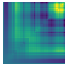
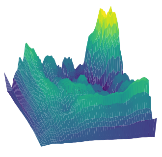
Figure 3. A realization of a Gaussian field with covariance $Q(\cdot,\cdot)$ defined in (2.19). The covariance structure is different from the Gaussian field ${\mathcal{M}}$, to be compared with Figure 1.

2.5.4. About other models with long-range correlated disorder

The question of the influence of disorder with long-range correlations on physical systems has been addressed widely in the physical literature, starting with the seminal paper by Weinrib and Halperin [71]. In [71], the authors propose a modification of Harris’ predictions on disorder relevance, depending on the rate of decay of the two-point correlation function: namely, if the disorder verifies $\mathbb{E}[\omega_{x}\omega_{y}]\asymp\|x-y\|^{-a}$ for some $a>0$, then disorder should be irrelevant if $\nu>2/\min(d,a)$ and relevant if $\nu<2/\min(d,a)$, with $\nu$ the critical exponent of the homogeneous model. In other words, Harris’ criterion is modified if $a<d$.

As far as the standard (one-dimensional) pinning model is concerned, this question has been investigated in the mathematical literature, for instance in [6, 7, 12, 16, 17, 31, 60]. In particular, it has been proven in [7, 12] that Weinrib–Halperin’s prediction fail: disorder becomes always relevant as soon as $a<d=1$. The main idea is that the two-point correlations do not encapsulate the important features of the environment; instead one has to study the rare appearance of large regions of favorable disorder. However, one could still hope to recover Weinrib–Halperin’s predictions for the existence of a non-trivial intermediate disorder scaling limit of the model (at least for Gaussian disorder), tuning down the inverse temperature $\beta_{n}\downarrow 0$ at the correct scale.

As a first step, one would need to make sense of the following continuum partition function, which is the natural candidate for the limit of the (free) partition function:

(2.20) $$\mathbf{Z}_{\beta}(t)=1+\sum_{k=1}^{\infty}\beta^{k}\int_{0<s_{1}<\cdots<s_{k}<t}\prod_{i=1}^{k}\vartheta(s_{i}-s_{i-1})\prod_{i=1}^{k}W(\mathrm{d}s_{i})\,.$$

In the above expression, $\vartheta(s)=s^{\alpha-1}$ corresponds to the scaled renewal mass function $\mathbf{P}(i\in\tau)$ (with $\alpha\in(0,1)$ the tail exponent of $\mathbf{P}(\tau_{1}>i)$, verifying $\alpha=1/\nu$) and $W$ a fractional Brownian Motion with Hurst index $H\in(\frac{1}{2},1)$, i.e. a Gaussian field with covariance function $\mathbb{E}[W_{s}W_{t}]=\frac{1}{2}(|s|^{2H}+|t|^{2H}-|t-s|^{2H})$, which corresponds to the scaling limit of a Gaussian field $(\omega_{n})_{n\in\mathbb{Z}}$ with correlations $\mathbb{E}[\omega_{n},\omega_{n+k}]\sim c|k|^{-a}$, $a=2(1-H)\in(0,1)$. Then, one is able to compute (or at least estimate) the $L^{2}$ norm of each term in the sum. In particular, for $k=1$, one gets

$$\left\|\int_{0<s<t}\vartheta(s)W(\mathrm{d}s)\right\|_{L^{2}}^{2}=c_{H}\int_{0<s^{\prime}<s<1}\!\!\!s^{\prime\alpha-1}s^{\alpha-1}(s-s^{\prime})^{2H-2}\mathrm{d}s\mathrm{d}s^{\prime}=c_{H}\frac{\Gamma(\alpha)\Gamma(2H-1)}{\Gamma(\alpha+2H-1)}\int_{0}^{1}s^{2\alpha+2H-3}\mathrm{d}s\,,$$

which is finite if and only if $2\alpha+2H-2=2/\nu-a>0$, that is if and only if $\nu<2/a$, recovering Weinrib–Halperin’s condition for disorder relevance. This suggests that the expansion (2.20) makes sense when $\nu<2/a$. However, when controlling the $L^{2}$ norm of the $k$-th term, we obtain a bound that is not summable in $k$. Therefore new ideas are needed in order to decide whether it is possible to make sense of (2.20) when $\nu<2/a$; if so, this would confirm Weinrib–Halperin’s predictions, in the sense put forward in [26].

Let us also mention that the effect of long-range correlations in the disorder has been studied in the directed polymer model, for instance in [55, 63]. However, in these references, the disorder displays correlations only in the spatial dimension and not in the time dimension; it remains an open problem to study the model with correlations in time.

2.6. Organisation of the rest of the paper

Henceforth, the paper is organized as follows. In Section 3 we prove Lemma 2.4, from which we deduce the convergence of arbitrary moments of the rescaled field $M_{n}$ to those of ${\mathcal{M}}$. Theorem 2.7 then follows from standard arguments of finite-dimensional convergence and tightness. Let us also mention that Claim 3.5 below ensures us that in the remainder of the paper, we may reduce all questions of convergence, notably the main theorem, to $L^{2}$-convergences on a convenient $L^{2}(\mathbb{P})$ space.

In Section 4, we discuss the integration against the random field ${\mathcal{M}}$. We first provide general results for defining the integral against a random field by using its covariance measure, notably Theorem 4.8. In Section 4.2 we apply these to prove the well-posedness of $\int\varphi\,\mathrm{d}{\mathcal{M}}$ in (2.5), and in Section 4.3 we proceed similarly for iterated integrals. In particular we prove that the series $\mathbf{Z}$ in (2.13) is a well-defined $L^{2}(\mathbb{P})$ random variable.

Section 5 contains the most technical parts of the paper, which are required to prove Theorem 2.8. Section 5.1 shows that we may reduce the statement to the case $h_{n}\equiv 0$, Sections 5.2–5.3 prove the convergence of any term of the polynomial expansion (2.1) to its continuous counterpart in (2.13), and Section 5.4 concludes with the convergence of the whole partition function to the series $\mathbf{Z}$.

Finally, Section 6 displays the proofs of statements regarding the homogeneous gPS model (Proposition 2.3), and when the limit is trivial (Proposition 2.10). Those results are postponed to the end of the paper since they rely on standard techniques, namely Riemann-sum convergences and estimates on bi-variate renewal processes.

Some estimates on bi-variate renewal processes and bivariate homogeneous pinning models are recalled in Appendix A. In Appendix B we prove Theorem 4.8: similar results can already be found in the literature (see e.g. [70, Theorem 2.5]), but for the sake of completeness we provide a full construction of the integral with covariance measures. In Appendix C we eventually provide examples of disorder distributions in $\mathfrak{P}_{4}$, $\mathfrak{P}_{8}$, as claimed in Example 2.6.

3. Convergence of the field $M_{n}$ to ${\mathcal{M}}$: proof of Theorem 2.7

Let us comment on the meaning of the convergence in Theorem 2.7. Define

(3.1) $$L^{\infty}([{\boldsymbol{0}},\textbf{{t}}])\,:=\,\big{\{}f:[{\boldsymbol{0}},\textbf{{t}}]\to\mathbb{R}\ ;\ \text{$f$ is measurable and bounded}\big{\}}\,,$$

and equip it with the norm $\|\cdot\|_{\infty}$ (and ensuing Borel sigma-algebra). Then, for any random variables $(W_{n})_{n\geq 1}$ and ${\mathcal{W}}$ in $L^{\infty}([{\boldsymbol{0}},\textbf{{t}}])$, we have that $W_{n}$ converges in distribution to ${\mathcal{W}}$ if for any bounded function $h:L^{\infty}([{\boldsymbol{0}},\textbf{{t}}])\to\mathbb{R}$ that is continuous (for the aforementioned topology), $\lim_{n\to\infty}\mathbb{E}[h(W_{n})]=\mathbb{E}[h({\mathcal{W}})]$. Notice that the fields $M_{n}$ and ${\mathcal{M}}$ defined above are a.s. bounded so this convergence is well-posed. In this section, we prove the convergence in Theorem 2.7 and we also provide useful estimates on $(M_{n}(\textbf{{s}}))_{\textbf{{s}}\succcurlyeq{\boldsymbol{0}}}$.

To be able to distinguish the different notation, the $L^{p}$ norms on spaces of functions from $[{\boldsymbol{0}},\textbf{{t}}]$ to $\mathbb{R}$, i.e. $L^{p}([{\boldsymbol{0}},\textbf{{t}}])$, will be noted $\|\cdot\|_{p}$, whereas on spaces of real random variables, i.e. $L^{p}(\mathbb{P})$, they will be noted $\|\cdot\|_{L^{p}(\mathbb{P})}$ or $\|\cdot\|_{L^{p}}$, $p\in[1,\infty]$.

3.1. Preliminary results: the covariance structure

We start with some preliminaries, controlling the covariances of the field $(\zeta_{\textbf{{i}}})_{\textbf{{i}}\in\mathbb{N}^{2}}$: we prove Lemma 2.4, then we show how the covariance function $K(\textbf{{u}},\textbf{{v}})$ appears and prove some other useful estimates. Recall that $\zeta_{\textbf{{i}}}=\zeta_{\textbf{{i}}}(\beta_{n}):=e^{\beta_{n}\omega_{\textbf{{i}}}-\lambda(\beta_{n})}-1$ has mean $0$, that $\omega_{\textbf{{i}}}=V(\widehat{\omega}_{i_{1}},\bar{\omega}_{i_{2}})$. Recall also the definition (2.8) of the sets $(\mathfrak{P}_{r})_{r\geq 1}$ and $\mathfrak{P}_{\infty}$ partitioning the set $\mathfrak{P}$ of all distributions.

Proof of Lemma 2.4.

First of all, if $i_{1}\neq j_{1}$ and $i_{2}\neq j_{2}$, then $\omega_{\textbf{{i}}}$ and $\omega_{\textbf{{j}}}$ are independent, so we clearly have that $\mathbb{E}[\zeta_{\textbf{{i}}}\zeta_{\textbf{{j}}}]=0$.

When $\textbf{{i}}=\textbf{{j}}$, by a simple (and classical) Taylor expansion, we find

$$\mathbb{E}[\zeta_{\textbf{{i}}}\zeta_{\textbf{{j}}}]=e^{\lambda(2\beta_{n})-2\lambda(\beta_{n})}-1\sim\mathbb{V}\mathrm{ar}(\omega_{{\boldsymbol{1}}})\beta_{n}^{2}\qquad\text{ as }\beta_{n}\downarrow 0\,.$$

It remains to treat the case $\textbf{{i}}\leftrightarrow\textbf{{j}}$ but $\textbf{{i}}\neq\textbf{{j}}$. Let us assume that $i_{1}\neq j_{1}$ but $i_{2}=j_{2}$ and write for simplicity $\varpi_{1}:=\widehat{\omega}_{i_{1}}$, $\varpi_{2}:=\bar{\omega}_{i_{2}}$ and $\varpi_{3}=\widehat{\omega}_{j_{1}}$: this way we have $\omega_{\textbf{{i}}}=V(\varpi_{1},\varpi_{2})$ and $\omega_{\textbf{{j}}}=V(\varpi_{2},\varpi_{3})$. Then, we write

(3.2) $$\begin{split}e^{2\lambda(\beta_{n})}\mathbb{E}[\zeta_{\textbf{{i}}}\zeta_{\textbf{{j}}}]&=\mathbb{E}[e^{\beta_{n}(V(\varpi_{1},\varpi_{2})+V(\varpi_{2},\varpi_{3}))}]-\mathbb{E}[e^{\beta_{n}V(\varpi_{1},\varpi_{2})}]\mathbb{E}[e^{\beta_{n}V(\varpi_{1},\varpi_{2})}]\\ &=\sum_{k=0}^{+\infty}\frac{\beta_{n}^{k}}{k!}\sum_{j=0}^{k}\binom{k}{j}\big{(}a_{j,k}-b_{j,k}\big{)}\,,\end{split}$$

where for the last equality we have expanded the exponentials, developed $(V(\varpi_{1},\varpi_{2})+V(\varpi_{2},\varpi_{3}))^{k}$ and set

$$a_{j,k}:=\mathbb{E}[V(\varpi_{1},\varpi_{2})^{j}V(\varpi_{2},\varpi_{3})^{k-j}]\,,\quad b_{j,k}:=\mathbb{E}[V(\varpi_{1},\varpi_{2})^{j}]\mathbb{E}[V(\varpi_{2},\varpi_{3})^{k-j}]\,.$$

Now, we show that for $\mathbb{P}\in\mathfrak{P}_{r}$, if $j<r$ then $a_{j,k}=b_{j,k}$ (and similarly for $k-j<r$, by symmetry). Indeed, by definition of $\mathfrak{P}_{r}$ the random variable $\mathbb{E}[V(\varpi_{1},\varpi_{2})^{j}\,|\,\varpi_{1}]$ is constant a.s., equal to $\mathbb{E}[V(\varpi_{1},\varpi_{2})^{j}]$. Therefore, if $j<r$, conditioning with respect to $\varpi_{1}$ we get

$$\begin{split}a_{j,k}=\mathbb{E}[V(\varpi_{1},\varpi_{2})^{j}V(\varpi_{2},\varpi_{3})^{k-j}]&=\mathbb{E}[\mathbb{E}[V(\varpi_{1},\varpi_{2})^{j}\,|\,\varpi_{1}]\,V(\varpi_{2},\varpi_{3})^{k-j}]\\ &=\mathbb{E}[V(\varpi_{1},\varpi_{2})^{j}]\mathbb{E}[V(\varpi_{2},\varpi_{3})^{k}]=b_{j,k}\,.\end{split}$$

Note that this also holds if $r=+\infty$.

Therefore, if $\mathbb{P}\in\mathfrak{P}_{\infty}$, we have $a_{j,k}=b_{j,k}$ for all $j,k\geq 0$, so $\mathbb{E}[\zeta_{\textbf{{i}}}\zeta_{\textbf{{j}}}]=0$, as announced. If $\mathbb{P}\in\mathfrak{P}_{r}$ with $r\in\mathbb{N}$, then we have $\sum_{j=0}^{k}\binom{k}{j}(a_{j,k}-b_{j,k})=0$ for all $k<2r$, and for $k=2r$, $\sum_{j=0}^{2r}\binom{k}{j}(a_{j,k}-b_{j,k})=\binom{2r}{r}(a_{r,r}-b_{r,r})$, with

$$\begin{split}a_{r,r}-b_{r,r}&=\mathbb{E}[V(\varpi_{1},\varpi_{2})^{r}V(\varpi_{2},\varpi_{3})^{r}]-\mathbb{E}[V(\varpi_{1},\varpi_{2})^{r}]\mathbb{E}[V(\varpi_{2},\varpi_{3})^{r}]\\ &=\mathbb{E}\big{[}\mathbb{E}[V(\varpi_{1},\varpi_{2})^{r}\,|\,\varpi_{2}]^{2}\big{]}-\mathbb{E}[V(\varpi_{1},\varpi_{2})^{r}]^{2}\\ &=\mathbb{V}\mathrm{ar}\big{(}\mathbb{E}[V(\varpi_{1},\varpi_{2})^{r}\,|\,\varpi_{2}]\big{)}=:\widetilde{\sigma}_{r}^{2}\,,\end{split}$$

where we have used that conditionally on $\varpi_{2}$, $V(\varpi_{1},\varpi_{2})$ and $V(\varpi_{2},\varpi_{3})$ are independent, and by symmetry of $V$ we have $\mathbb{E}[V(\varpi_{1},\varpi_{2})^{r}\,|\,\varpi_{2}]=\mathbb{E}[V(\varpi_{2},\varpi_{3})^{r}\,|\,\varpi_{2}]$. Going back to (3.2), for $\mathbb{P}\in\mathfrak{P}_{r}$, we get that as $\beta_{n}\downarrow 0$,

$$e^{2\lambda(\beta_{n})}\mathbb{E}[\zeta_{\textbf{{i}}}\zeta_{\textbf{{j}}}]=(1+o(1))\frac{\beta_{n}^{2r}}{(2r)!}\binom{2r}{r}\widetilde{\sigma}_{r}^{2}=(1+o(1))\frac{\widetilde{\sigma}_{r}^{2}}{(r!)^{2}}\beta_{n}^{2r}\,.$$

Since $e^{2\lambda(\beta_{n})}\to 1$, this concludes the proof of Lemma 2.4 with $\sigma^{2}_{r}:=\widetilde{\sigma}^{2}_{r}/(r!)^{2}$. ∎

Let us define, for $\textbf{{s}}\in\mathbb{R}_{+}\times\mathbb{R}_{+}$,

(3.3) $$\overline{M}_{n}(\textbf{{s}}):=\frac{1}{\sigma_{r}n^{3/2}\beta_{n}^{r}}M_{n}(\textbf{{s}})=\frac{1}{\sigma_{r}n^{3/2}\beta_{n}^{r}}\sum_{\textbf{{i}}\in\llbracket{\boldsymbol{1}},n\textbf{{s}}\rrbracket}\zeta_{\textbf{{i}}}\,,$$

where $\frac{1}{\sigma_{r}n^{3/2}\beta_{n}^{r}}$ is the scaling advertised in Theorem 2.7. Thanks to Lemma 2.4, we easily identify the covariance structure of $(\overline{M}_{n}(\textbf{{s}}))_{\textbf{{s}}\succcurlyeq{\boldsymbol{0}}}$. Let $\textbf{{s}}=(s_{1},s_{2}),\textbf{{t}}=(t_{1},t_{2})\in\mathbb{R}_{+}^{2}$, and let us compute

(3.4) $$\mathbb{E}\left[\overline{M}_{n}(\textbf{{s}})\overline{M}_{n}(\textbf{{t}})\right]=\frac{1}{\sigma_{r}^{2}n^{3}\beta_{n}^{2r}}\sum_{\textbf{{i}}\in\llbracket{\boldsymbol{1}},n\textbf{{s}}\rrbracket}\sum_{\textbf{{j}}\in\llbracket{\boldsymbol{1}},n\textbf{{t}}\rrbracket}\mathbb{E}\left[\zeta_{\textbf{{i}}}\zeta_{\textbf{{j}}}\right].$$

Then, in view of Lemma 2.4 (or (2.7)), we distinguish in the sum indices $(\textbf{{i}},\textbf{{j}})$ that are equal (there are $(1+o(1))(s_{1}\wedge t_{1})(s_{2}\wedge t_{2})\,n^{2}$ of them), aligned indices that are not equal (there are $(1+o(1))(s_{1}\wedge t_{1})(s_{2}\wedge t_{2})(s_{1}\vee t_{1}+s_{2}\vee t_{2})\,n^{3}$ of them, see Figure 4), and other indices (which do not contribute to the sum).

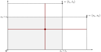
Figure 4. Graphical representation of indices $\textbf{{i}}\in\llbracket{\boldsymbol{1}},n\textbf{{s}}\rrbracket$, $\textbf{{j}}\in\llbracket{\boldsymbol{1}},n\textbf{{t}}\rrbracket$ with $\textbf{{i}}\leftrightarrow\textbf{{j}}$ and $\textbf{{i}}\neq\textbf{{j}}$. One of $\textbf{{i}},\textbf{{j}}$ must be in $\llbracket{\boldsymbol{1}},n\textbf{{s}}\rrbracket\cap\llbracket{\boldsymbol{1}},n\textbf{{t}}\rrbracket$ (there are $(s_{1}\wedge t_{1})(s_{2}\wedge t_{2})n^{2}$ possible locations, represented as the red dot), and the other one has to be aligned with it (there are $(s_{1}\vee t_{1}+s_{2}\vee t_{2})n-1$ possibilities, represented by the red lines).

Therefore, in view of (2.7), as $n\to+\infty$ the covariance $\mathbb{E}\big{[}\overline{M}_{n}(\textbf{{s}})\overline{M}_{n}(\textbf{{t}})\big{]}$ is asymptotic to

$$(s_{1}\wedge t_{1})(s_{2}\wedge t_{2})\frac{\sigma^{2}}{\sigma_{r}^{2}n\beta_{n}^{2r}}\hskip 1.0pt+\hskip 1.0pt(s_{1}\wedge t_{1})(s_{2}\wedge t_{2})(s_{1}\vee t_{1}+s_{2}\vee t_{2})\,.$$

If $\lim_{n\to\infty}n\beta_{n}^{2r}=+\infty$, which is one assumption of Theorem 2.7, then we end up with

(3.5) $$\lim_{n\to+\infty}\mathbb{E}\left[\overline{M}_{n}(\textbf{{s}})\overline{M}_{n}(\textbf{{t}})\right]=K(\textbf{{s}},\textbf{{t}}):=(s_{1}\wedge t_{1})(s_{2}\wedge t_{2})(s_{1}\vee t_{1}+s_{2}\vee t_{2}),$$

which is the correlation function in Theorem 2.7.

Let us conclude this section by giving a lemma that gives estimates on multi-point correlations—this will appear useful in the rest of the paper. Let us define the classes of sets of “$m$-aligned” indices (with possible repetitions of the indices) as

(3.6) $$\mathcal{A}_{m}:=\left\{(\textbf{{i}}_{1},\ldots,\textbf{{i}}_{m})\in(\mathbb{N}^{2})^{m}\ ;\ \begin{aligned} &\forall\ 1\leq k,k^{\prime}\leq m,\exists k_{0}=k,k_{1},\ldots,k_{p}=k^{\prime}\\ &\text{such that }\forall 1\leq a\leq p,\ \textbf{{i}}_{k_{a}}\leftrightarrow\textbf{{i}}_{k_{a-1}}\end{aligned}\right\}\,,$$

in other words, $(\textbf{{i}}_{1},\ldots,\textbf{{i}}_{m})\in\mathcal{A}_{m}$ if for all pair $(\textbf{{i}}_{k},\textbf{{i}}_{k^{\prime}})$, $1\leq k,k^{\prime}\leq m$, there is a path from $\textbf{{i}}_{k}$ to $\textbf{{i}}_{k^{\prime}}$ of subsequently aligned indices in $\{\textbf{{i}}_{1},\ldots,\textbf{{i}}_{m}\}$. We refer to Figure 5 below for an illustration of sets that are $m$-aligned.

Moreover, a specific type of $m$-aligned sets will play an important role in the computation of the scaling limit of the partition function below, which may be formed by the union of two renewal trajectories $\boldsymbol{\tau},\boldsymbol{\tau}^{\prime}\subset\mathbb{N}^{2}$. A $m$-aligned set $(\textbf{{i}}_{1},\ldots,\textbf{{i}}_{m})\in{\mathcal{A}}_{m}$ is called a $m$-chain of points if there is no repetition of the indices and if we may reorder it into a non-decreasing sequence $\textbf{{i}}_{1}\preccurlyeq\textbf{{i}}_{2}\preccurlyeq\textbf{{i}}_{3}\preccurlyeq\ldots$ such that $\textbf{{i}}_{1}\prec\textbf{{i}}_{3}\prec\cdots$ and $\textbf{{i}}_{2}\prec\textbf{{i}}_{4}\prec\cdots$; an example is provided in Figure 5. For such sets, we improve our estimate on multi-point correlations by additionally controlling the dependence of the pre-factor in $m\in\mathbb{N}$.

Figure 5. Examples of sets that are $m$-aligned with $m=7$. The indices that are alone on their column or on their line are represented with (empty) circles, the ones that are aligned with another index both vertically and horizontally are represented by filled dots. If we denote $b$ the number of points alone on their line or column then we have from left to right $b=5$, $b=0$, $b=2$. More specifically, the third example is a $m$-chain of points.

Lemma 3.1.

Assume that $\mathbb{P}\in\mathfrak{P}_{r}$ for some $r\in\mathbb{N}$. For any $m\geq 2$ and $q_{1},\ldots,q_{m}\in\mathbb{N}$, there is a constant $C=C_{m,q}$ such that for any set $\textbf{{I}}=(\textbf{{i}}_{1},\textbf{{i}}_{2},\ldots,\textbf{{i}}_{m})\in{\mathcal{A}}_{m}$ of distinct $m$-aligned points we have

(3.7) $$0\leq\mathbb{E}\Big{[}\prod_{p=1}^{m}\zeta_{\textbf{{i}}_{p}}^{q_{p}}\Big{]}\leq C\,\beta_{n}^{R}\qquad\text{with }R:=\sum_{p=1}^{m}q_{p}\vee r_{p}\,,$$

where $r_{p}:=r$ if $\textbf{{i}}_{p}$ is alone on its line or on its column (in other words if $\textbf{{i}}_{p}^{(2)}\neq\textbf{{i}}_{j}^{(2)}$ for all $j\neq p$ or if $\textbf{{i}}_{p}^{(1)}\neq\textbf{{i}}_{j}^{(1)}$ for all $j\neq p$), and $r_{p}=\lceil\frac{r}{2}\rceil$ otherwise.

In addition, there exists a constant $C^{\prime}>0$ such that for any $m\geq 2$, for any $m$-chain of points $\textbf{{I}}=(\textbf{{i}}_{1},\textbf{{i}}_{2},\ldots,\textbf{{i}}_{m})\in{\mathcal{A}}_{m}$, we have

(3.8) $$0\leq\mathbb{E}\Big{[}\prod_{p=1}^{m}\zeta_{\textbf{{i}}_{p}}\Big{]}\leq(C^{\prime})^{m}\beta_{n}^{2r+(m-2)\lceil\frac{r}{2}\rceil}\,.$$

Proof.

The fact that correlations are non-negative simply follows from the observation that $\omega\mapsto e^{\beta_{n}\omega-\lambda(\beta_{n})}-1$ is non-decreasing and from the FKG inequality (see e.g. [62]), so we only have to prove the upper bound.

Let us write for simplicity $\varpi_{p,1}=\widehat{\omega}_{i_{p}^{(1)}}$, $\varpi_{p,2}=\bar{\omega}_{i_{p}^{(2)}}$: this way, we have $\omega_{\textbf{{i}}_{p}}=V(\varpi_{p,1},\varpi_{p,2})$. Therefore, we can write

(3.9) $$e^{\lambda(\beta_{n})}\zeta_{\textbf{{i}}_{p}}=e^{\beta_{n}V(\varpi_{p,1},\varpi_{p,2})}-\mathbb{E}[e^{\beta_{n}V(\varpi_{p,1},\varpi_{p,2})}]=\sum_{k=0}^{+\infty}\frac{\beta_{n}^{k}}{k!}\Big{(}V(\varpi_{p,1},\varpi_{p,2})^{k}-\mathbb{E}\big{[}V(\varpi_{p,1},\varpi_{p,2})^{k}\big{]}\Big{)}\,.$$

Hence, expanding the power $q_{p}$ we have

$$\Big{(}e^{\lambda(\beta_{n})}\zeta_{\textbf{{i}}_{p}}\Big{)}^{q_{p}}=\sum_{\ell=0}^{+\infty}\beta_{n}^{\ell}W_{p,\ell}$$

where we have set

$$W_{p,\ell}:=\sum_{k_{1}+\cdots+k_{q_{p}}=\ell}\frac{1}{\prod_{j=1}^{q_{p}}k_{j}!}\prod_{j=1}^{q_{p}}\Big{(}V(\varpi_{p,1},\varpi_{p,2})^{k_{j}}-\mathbb{E}\big{[}V(\varpi_{p,1},\varpi_{p,2})^{k_{j}}\big{]}\Big{)}\,,$$

and notice that $W_{p,\ell}=0$ for any $\ell<q_{p}$. We can now expand the product of series and take the expectation: we get that

(3.10) $$e^{\sum_{p=1}^{m}q_{p}\lambda(\beta_{n})}\mathbb{E}\Big{[}\prod_{p=1}^{m}\zeta_{\textbf{{i}}_{p}}^{q_{p}}\Big{]}=\sum_{\ell=0}^{+\infty}\beta_{n}^{\ell}\sum_{\ell_{1}+\cdots+\ell_{m}=\ell}\mathbb{E}\Big{[}\prod_{j=1}^{m}W_{j,\ell_{j}}\Big{]}\,.$$

Now, using that for any $k<r$ $\mathbb{E}[V(\varpi_{p,1},\varpi_{p,2})^{k}\,|\,\varpi_{p,2}]=\mathbb{E}[V(\varpi_{p,1},\varpi_{p,2})^{k}]$ a.s. by definition of $\mathfrak{P}_{r}$, one can easily check that $\mathbb{E}[W_{p,\ell}\,|\,\varpi_{p,2}]=0$ a.s. for any $\ell<r$. With this in mind, if $\textbf{{i}}_{p}$ is alone on its line (i.e. $\textbf{{i}}_{p}^{(2)}\neq\textbf{{i}}_{j}^{(2)}$ for all $j\neq p$), since $\varpi_{p,1}$ appears only in $W_{p,\ell_{p}}$, conditioning with respect to $(\varpi_{j,1})_{j\neq p}$ and $(\varpi_{j,2})_{1\leq j\leq m}$, we get

$$\mathbb{E}\Big{[}\prod_{j=1}^{m}W_{j,\ell_{j}}\Big{]}=\mathbb{E}\Big{[}\mathbb{E}[W_{p,\ell_{p}}\,|\,\varpi_{p,2}]\prod_{j=1,j\neq p}^{m}W_{j,\ell_{j}}\Big{]}=0\quad\text{ if }\ell_{p}<r\,.$$

This obviously holds also in the case where $\textbf{{i}}_{p}$ is alone on its column since then $\varpi_{p,2}$ appears only in $W_{p,\ell_{p}}$. However, we cannot use the same trick if both $\varpi_{p,1}$ and $\varpi_{p,2}$ appear in other terms $W_{j,\ell_{j}}$ with $j\neq p$: in that case, we use Cauchy–Schwarz inequality to get

$$\Big{|}\mathbb{E}\Big{[}\prod_{j=1}^{m}W_{j,\ell_{j}}\Big{]}\Big{|}\leq\mathbb{E}\Big{[}W_{p,\ell_{p}}^{2}\Big{]}^{1/2}\mathbb{E}\Big{[}\prod_{j\neq p}W_{j,\ell_{j}}^{2}\Big{]}^{1/2}=0\quad\text{ if }2\ell_{p}<r\,.$$

where we have used that, analogously as above, $\mathbb{E}[(W_{p,\ell})^{2}\,|\,\varpi_{p,2}]=0$ a.s. for any $2\ell<r$.

Overall, we get that $\mathbb{E}[\prod_{j=1}^{m}W_{j,\ell_{j}}]=0$ if there is some $j$ such that $\ell_{j}<q_{j}\vee r_{j}$, with $r_{j}$ as defined in the statement of the lemma. Therefore, the first non-zero term in the series (3.10) is (possibly) for $\ell_{j}=q_{j}\vee r_{j}$: and since $\exp(-\lambda(\beta_{n}))$ is bounded by $1$, this concludes the proof of (3.7).

For the second part of the lemma (in which $q_{p}=1$ for all $p$), note that starting from (3.9), we have similarly to (3.10)

(3.11) $$e^{m\lambda(\beta_{n})}\mathbb{E}\Big{[}\prod_{p=1}^{m}\zeta_{\textbf{{i}}_{p}}\Big{]}=\sum_{k_{1},\cdots,k_{m}\geq 0}\frac{(\beta_{n})^{k_{1}+\cdots+k_{m}}}{\prod_{p=1}^{m}k_{p}!}\mathbb{E}\Big{[}\prod_{p=1}^{m}Y_{p,k_{p}}\Big{]}\,,$$

with $Y_{p,k}:=V(\varpi_{p,1},\varpi_{p,2})^{k}-\mathbb{E}\big{[}V(\varpi_{p,1},\varpi_{p,2})^{k}\big{]}$. Then, exactly as above, the sum can be restricted to $k_{p}\geq r_{p}$ for all $p$, with here $r_{1}=r_{m}=r$ (the first and last index of the chain are both aligned with only one other index), and otherwise $r_{p}=\lceil\frac{r}{2}\rceil$ for $2\leq p\leq m-1$. Now, note that, using Cauchy–Schwarz inequality, we get that

$$\mathbb{E}\Big{[}\prod_{p=1}^{m}Y_{p,k_{p}}\Big{]}\leq\mathbb{E}\Big{[}\prod_{p\text{ even}}(Y_{p,k_{p}})^{2}\Big{]}^{1/2}\mathbb{E}\Big{[}\prod_{p\text{ odd}}(Y_{p,k_{p}})^{2}\Big{]}^{1/2}\leq\prod_{p=1}^{m}\mathbb{E}\big{[}(Y_{p,k_{p}})^{2}\big{]}^{1/2}\,,$$

where we used that $(Y_{p,k_{p}})_{p\text{ even}}$, resp. $(Y_{p,k_{p}})_{p\text{ odd}}$, are independent, thanks to the structure of I (the indices $\textbf{{i}}_{p}$ for $p$ even, resp. $p$ odd, are strictly increasing). Since by assumption $V(\varpi_{p,1},\varpi_{p,2})$ admits a finite $\beta_{0}/2$ exponential moment, we get that there is a constant $C>0$ such that $\mathbb{E}[V(\varpi_{p,1},\varpi_{p,2})^{k}]\leq C^{k}$ for all $k\geq 1$, hence $\mathbb{E}[(Y_{p,k_{p}})^{2}]^{1/2}\leq(C^{\prime})^{k_{p}}$. We therefore end up with

$$\mathbb{E}\Big{[}\prod_{p=1}^{m}\zeta_{\textbf{{i}}_{p}}\Big{]}=\sum_{k_{1}\geq r_{1},\cdots,k_{m}\geq r_{m}}\frac{(C^{\prime}\beta_{n})^{k_{1}+\cdots+k_{m}}}{\prod_{p=1}^{m}k_{p}!}\leq(C^{\prime}\beta_{n})^{\sum_{i=1}^{m}r_{i}}e^{mC^{\prime}\beta_{n}}\,,$$

where we used that $\sum_{k\geq r}\frac{a^{k}}{k!}\leq a^{r}\sum_{k\geq 0}\frac{a^{k}}{k!}=a^{r}e^{a}$ for $a\geq 0$. Recalling that we already observed above that $\sum_{i=1}^{m}r_{i}=2r+(m-2)\lceil\frac{r}{2}\rceil$, this concludes the proof of (3.8). ∎

3.2. Finite-dimensional convergence

In this section, we prove the convergence in distribution of $(\overline{M}_{n}(\textbf{{s}}_{1}),\ldots,\overline{M}_{n}(\textbf{{s}}_{m}))$, for any $m\in\mathbb{N}$ and $\textbf{{s}}_{1},\ldots,\textbf{{s}}_{m}\in\mathbb{R}_{+}^{2}$. Let $\Sigma_{\textbf{{s}}_{1},\ldots,\textbf{{s}}_{m}}(i,j):=K(\textbf{{s}}_{i},\textbf{{s}}_{j})$ be the covariance matrix of $({\mathcal{M}}(\textbf{{s}}_{1}),\ldots,{\mathcal{M}}(\textbf{{s}}_{m}))$, where we recall that $K(\cdot,\cdot)$ is defined in (2.11). In view of (3.5), $\Sigma$ is the limit of the sequence of the covariance matrices of $(\overline{M}_{n}(\textbf{{s}}_{1}),\ldots,\overline{M}_{n}(\textbf{{s}}_{m}))$; in particular, it is positive semi-definite.

Proposition 3.2.

Let $m\in\mathbb{N}$ and $\textbf{{s}}_{1},\ldots,\textbf{{s}}_{m}\in\mathbb{R}_{+}^{2}$. As $n\to\infty$, if $lim_{n\to\infty}\beta_{n}=0$ and $\lim_{n\to\infty}n\beta_{n}^{2r}=+\infty$, then $(\overline{M}_{n}(\textbf{{s}}_{1}),\ldots,\overline{M}_{n}(\textbf{{s}}_{m}))$ converges in distribution toward a Gaussian vector, centered and with covariance matrix $\Sigma_{\textbf{{s}}_{1},\ldots,\textbf{{s}}_{m}}$.

Before we prove this proposition, let us start with the case $m=1$, which already encapsulates the combinatorial difficulty and will ease the understanding of the general case $m\in\mathbb{N}$. We show the convergence of the moments of $\overline{M}_{n}(\textbf{{s}})$ to the moments of a Gaussian variable, which implies the convergence in distribution.

Lemma 3.3.

Let $\ell\in\mathbb{N}$ and $\textbf{{s}}\in\mathbb{R}_{+}^{2}$. Then $\mathbb{E}\big{[}(\overline{M}_{n}(\textbf{{s}}))^{\ell}\big{]}$ is well defined if $n$ is large enough, and if $lim_{n\to\infty}\beta_{n}=0$, $\lim_{n\to\infty}n\beta_{n}^{2r}=+\infty$, then we have

(3.12) $$\lim_{n\to+\infty}\mathbb{E}\Big{[}\big{(}\overline{M}_{n}(\textbf{{s}})\big{)}^{\ell}\Big{]}\>=\>\begin{cases}0&\quad\text{ if }\ell\text{ is odd},\\ \big{(}K(\textbf{{s}},\textbf{{s}})\big{)}^{\ell/2}\,\frac{\ell!}{2^{\ell/2}(\ell/2)!}&\quad\text{ if }\ell\text{ is even.}\end{cases}$$

where $K(\textbf{{s}},\textbf{{t}})$ is defined in (2.11), so $K(\textbf{{s}},\textbf{{s}})=s_{1}s_{2}(s_{1}+s_{2})$.

Proof.

We write

(3.13) $$\mathbb{E}\Big{[}\big{(}\overline{M}_{n}(\textbf{{s}})\big{)}^{\ell}\Big{]}=\Big{(}\frac{1}{\sigma_{r}n^{3/2}\beta_{n}^{r}}\Big{)}^{\ell}\sum_{\textbf{{i}}_{1}\in\llbracket{\boldsymbol{1}},n\textbf{{s}}\rrbracket}\cdots\sum_{\textbf{{i}}_{\ell}\in\llbracket{\boldsymbol{1}},n\textbf{{s}}\rrbracket}\mathbb{E}\left[\zeta_{\textbf{{i}}_{1}}\cdots\zeta_{\textbf{{i}}_{\ell}}\right].$$

Now, notice that $\mathbb{E}\left[\zeta_{\textbf{{i}}_{1}}\cdots\zeta_{\textbf{{i}}_{\ell}}\right]$ depends only on the relative positions of the indices $(\textbf{{i}}_{k})_{k=1}^{\ell}$. For instance, if one of the $\textbf{{i}}_{k}$ is isolated (i.e. not aligned with any other index i) then the expectation is equal to $0$.

Recall the definition (3.6) of classes of sets of “$m$-aligned” indices (with possible repetitions of the indices). Then, for any $\textbf{{I}}=(\textbf{{i}}_{1},\ldots,\textbf{{i}}_{\ell})\in\llbracket{\boldsymbol{1}},n\textbf{{s}}\rrbracket^{\ell}$, there is a unique partition $\mathbb{J}=\{J_{1},\ldots,J_{k}\}$ of $\{1,\ldots,\ell\}$ such that for $1\leq a\leq k$, $\{\textbf{{i}}_{j}\}_{j\in J_{a}}$ is a maximal set of “$m$-aligned” indices of I; in particular $\{\textbf{{i}}_{j}\}_{j\in J_{a}}\in{\mathcal{A}}_{|J_{a}|}$ for all $1\leq a\leq k$, and $\textbf{{i}}_{j}\not\leftrightarrow\textbf{{i}}_{j^{\prime}}$ for any $j\in J_{a}$, $j^{\prime}\in J_{b}$ with $a\neq b$. One can view $(J_{a})_{1\leq a\leq k}$ as equivalence classes, for the following equivalence relation (defined for I fixed): $j\rightleftarrows j^{\prime}$ if and only if there exists a path $j_{0}=j,j_{1},\ldots,j_{q}=j^{\prime}$ in $\{1,\ldots,\ell\}$ satisfying $\textbf{{i}}_{j_{p}}\leftrightarrow\textbf{{i}}_{j_{p+1}}$ for all $0\leq p<q$. For $\textbf{{I}}=(\textbf{{i}}_{1},\ldots,\textbf{{i}}_{\ell})\in\llbracket{\boldsymbol{1}},n\textbf{{s}}\rrbracket^{\ell}$, we denote $\Phi(\textbf{{I}})=\mathbb{J}$ this partition. For $J\subset\{1,\ldots,\ell\}$ we let $\Phi_{\textbf{{I}}}^{-1}(J)\subset\textbf{{I}}$ be the set $\{\textbf{{i}}_{j},j\in J\}$, with possible repetition of the indices: this way, any partition $\mathbb{J}=\{J_{1},\ldots,J_{k}\}$ of $\{1,\ldots,\ell\}$ induces a partition $\{\Phi_{\textbf{{I}}}^{-1}(J_{1}),\ldots,\Phi_{\textbf{{I}}}^{-1}(J_{s})\}$ of I; if $\mathbb{J}=\Phi(\textbf{{I}})$, this corresponds to the partitioning of I into maximal sets of “$m$-aligned” indices.

Therefore, if $\Phi(\textbf{{I}})=\mathbb{J}=\{J_{1},\ldots,J_{k}\}$, we may factorize

(3.14) $$\mathbb{E}\left[\zeta_{\textbf{{i}}_{1}}\cdots\zeta_{\textbf{{i}}_{\ell}}\right]=\prod_{a=1}^{k}\mathbb{E}\Big{[}\prod_{j\in J_{a}}\zeta_{\textbf{{i}}_{j}}\Big{]}=\prod_{J\in\mathbb{J}}\mathbb{E}\Big{[}\prod_{\textbf{{i}}\in\Phi_{\textbf{{I}}}^{-1}(J)}\zeta_{\textbf{{i}}}\Big{]}\,.$$

As a consequence, denoting ${\mathcal{J}}_{\ell}$ the set of partitions of $\{1,\ldots,\ell\}$, we write

(3.15) $$\mathbb{E}\big{[}(\overline{M}_{n}(\textbf{{s}}))^{\ell}\big{]}=\Big{(}\frac{1}{\sigma_{r}n^{3/2}\beta_{n}^{r}}\Big{)}^{\ell}\sum_{\mathbb{J}\in{\mathcal{J}}_{\ell}}\sum_{\begin{subarray}{c}\textbf{{I}}\in\llbracket{\boldsymbol{1}},n\textbf{{s}}\rrbracket^{\ell}\\ \Phi(\textbf{{I}})=\mathbb{J}\end{subarray}}\prod_{J\in\mathbb{J}}\mathbb{E}\Big{[}\prod_{\textbf{{i}}\in\Phi_{\textbf{{I}}}^{-1}(J)}\zeta_{\textbf{{i}}}\Big{]}\,.$$

First of all, in (3.15), we can restrict the sum to having only $|J|\geq 2$: indeed if $|J|=1$ we obviously have $\mathbb{E}[\prod_{\textbf{{i}}\in\Phi_{\textbf{{I}}}^{-1}(J)}\zeta_{\textbf{{i}}}]=\mathbb{E}[\zeta_{\boldsymbol{1}}]=0$ (note that it also restricts the sum to $|\mathbb{J}|\leq\ell/2$). Now, we claim that the main contribution in the sum comes from having $|J|=2$ for all $J\in\mathbb{J}$, or in other words from the term $|\mathbb{J}|=\ell/2$.

Indeed let us show that, for any $m\geq 3$,

(3.16) $$\frac{1}{(\sigma_{r}n^{3/2}\beta_{n}^{r})^{m}}\sum_{I\in{\mathcal{A}}_{m}(n\textbf{{s}})}\mathbb{E}\Big{[}\prod_{\textbf{{i}}\in I}\zeta_{\textbf{{i}}}\Big{]}\xrightarrow{n\to+\infty}0\,,$$

where we introduced the notation ${\mathcal{A}}_{m}(n\textbf{{s}})=\{I\in{\mathcal{A}}_{m},I\subset\llbracket{\boldsymbol{1}},n\textbf{{s}}\rrbracket\}$ (note that we still allow repetitions of the indices). To that end, we perform a first simplification: denote $\widetilde{\mathcal{A}}_{m}(n\textbf{{s}})$ the set of $I\in{\mathcal{A}}_{m}(n\textbf{{s}})$ such that all indices in $I$ are distinct. Then, we clearly have that $|{\mathcal{A}}_{m}\setminus\widetilde{\mathcal{A}}_{m}|\leq m|{\mathcal{A}}_{m-1}|\leq Cm\|\textbf{{s}}\|_{1}n^{m}$ and hence

$$\frac{1}{(\sigma_{r}n^{3/2}\beta_{n}^{r})^{m}}\sum_{I\in{\mathcal{A}}_{m}(n\textbf{{s}})\setminus\widetilde{\mathcal{A}}_{m}(n\textbf{{s}})}\mathbb{E}\Big{[}\prod_{\textbf{{i}}\in I}\zeta_{\textbf{{i}}}\Big{]}\leq C_{r,m}\frac{1}{(n^{1/2}\beta_{n}^{r})^{m}}\xrightarrow{n\to+\infty}0\,,$$

where we simply bounded $\mathbb{E}[\prod_{\textbf{{i}}\in I}\zeta_{\textbf{{i}}}]$ by a constant and used that $n\beta_{n}^{2r}\to+\infty$. We therefore only need to prove (3.16) with ${\mathcal{A}}_{m}(n\textbf{{s}})$ replaced by $\widetilde{\mathcal{A}}_{m}(n\textbf{{s}})$. Now, with the idea of using Lemma 3.1, let us define (see Figure 5 for an illustration)

$$\widetilde{\mathcal{A}}_{m}^{(b)}(n\textbf{{s}}):=\Big{\{}\{\textbf{{i}}_{1},\ldots,\textbf{{i}}_{m}\}\in\widetilde{\mathcal{A}}_{m}(n\textbf{{s}})\,,\text{ there are exactly $b$ indices alone on a line or a column}\Big{\}}\,.$$

Now we just have to show (3.16) with $\widetilde{\mathcal{A}}_{m}^{(b)}(n\textbf{{s}})$ in place of ${\mathcal{A}}_{m}(n\textbf{{s}})$, for any $b\in\{0,\ldots,m\}$. Using Lemma 3.1-(3.7), we then have that for an $I\in\widetilde{\mathcal{A}}_{m}^{(b)}(n\textbf{{s}})$ (recall all indices are distinct)

$$\mathbb{E}\Big{[}\prod_{\textbf{{i}}\in I}\zeta_{\textbf{{i}}}\Big{]}\leq C\beta_{n}^{br+(m-b)\lceil r/2\rceil}\leq C\beta_{n}^{(b+m)r/2}\,.$$

Hence, using that $|\widetilde{\mathcal{A}}_{m}^{(b)}(n\textbf{{s}})|\leq|{\mathcal{A}}_{m}(n\textbf{{s}})|\leq C\|\textbf{{s}}\|_{1}n^{m+1}$, we have

(3.17) $$\frac{1}{(\sigma_{r}n^{3/2}\beta_{n}^{r})^{m}}\sum_{I\in\widetilde{\mathcal{A}}_{m}^{(b)}(n\textbf{{s}})}\mathbb{E}\Big{[}\prod_{\textbf{{i}}\in I}\zeta_{\textbf{{i}}}\Big{]}\leq\frac{C_{m,r}}{(n^{1/2}\beta_{n}^{r})^{m}}n\beta_{n}^{(b+m)r/2}=\frac{C_{m,r}}{(n^{1/2}\beta_{n}^{r})^{m-2}}\beta_{n}^{(b+m-4)r/2}\,.$$

Now, this goes to $0$ since $m\geq 3$ and $n^{1/2}\beta_{n}^{r}\to\infty$, due also to the fact that $b+m\geq 4$: indeed, we cannot have $b=0$ if $m=3$ so we either have $b\geq 1$ or $m\geq 4$.

In addition to (3.16), recall that when $m=2$ then (3.5) shows that

$$(\sigma_{r}n^{3/2}\beta_{n}^{r})^{-m}\sum_{I\in{\mathcal{A}}_{m}(n\textbf{{s}})}\mathbb{E}\Big{[}\prod_{\textbf{{i}}\in I}\zeta_{\textbf{{i}}}\Big{]}\xrightarrow{n\to+\infty}K(\textbf{{s}},\textbf{{s}})\;,$$

in particular these terms are bounded. All together, for any fixed partition $\mathbb{J}\in{\mathcal{J}}_{\ell}$ with at least one $|J|\geq 3$, we have

(3.18) $$\begin{split}\frac{1}{(\sigma_{r}n^{3/2}\beta_{n}^{r})^{\ell}}&\sum_{\begin{subarray}{c}\textbf{{I}}\in\llbracket{\boldsymbol{1}},n\textbf{{s}}\rrbracket^{\ell}\\ \Phi(\textbf{{I}})=\mathbb{J}\end{subarray}}\prod_{J\in\mathbb{J}}\hskip 1.0pt\mathbb{E}\Big{[}\prod_{\textbf{{i}}\in\Phi_{\textbf{{I}}}^{-1}(J)}\zeta_{\textbf{{i}}}\Big{]}\leq\;\prod_{J\in\mathbb{J}}\Big{(}\frac{1}{(\sigma_{r}n^{3/2}\beta_{n}^{r})^{|J|}}\sum_{I\in{\mathcal{A}}_{|J|}(n\textbf{{s}})}\mathbb{E}\Big{[}\prod_{\textbf{{i}}\in I}\zeta_{\textbf{{i}}}\Big{]}\Big{)}\;\stackrel{{\scriptstyle n\to+\infty}}{{\longrightarrow}}\;0,\end{split}$$

where we simply dropped the condition that $\textbf{{i}}_{j}\not\leftrightarrow\textbf{{i}}_{j^{\prime}}$ if $j,j^{\prime}$ are in different $J$’s.

Recall (3.15), where we have already said that we can restrict the sum to $\mathbb{J}\in{\mathcal{J}}_{\ell}$ having all $|J|\geq 2$.

(i) If $\ell$ is odd, then it imposes that one $|J|$ is larger or equal than $3$. Hence $\mathbb{E}[(\overline{M}_{n}(\textbf{{s}}))^{\ell}]$ goes to $0$, which proves the first part of (3.12).

(ii) If $\ell$ is even, then the only part contributing to the sum in (3.15) comes from $\mathbb{J}\in{\mathcal{J}}_{\ell}$ having all $|J|=2$: we denote $\mathscr{P}_{\ell}$ the set of pairings of $\{1,\ldots,\ell\}$, i.e. the sets of partitions $\mathbb{J}\in{\mathcal{P}}_{\ell}$ with $|J|=2$ for all $J\in\mathbb{J}$. We end up with

(3.19) $$\mathbb{E}\big{[}(\overline{M}_{n}(\textbf{{s}}))^{\ell}\big{]} =o(1)+\frac{1}{n^{3\ell/2}}\sum_{\mathbb{J}\in\mathscr{P}_{\ell}}\sum_{\begin{subarray}{c}\textbf{{I}}\in\llbracket{\boldsymbol{1}},n\textbf{{s}}\rrbracket^{\ell}\\ \Phi(\textbf{{I}})=\mathbb{J}\end{subarray}}\prod_{J\in\mathbb{J}}\frac{1}{\sigma_{r}^{2}\beta_{n}^{2r}}\mathbb{E}\Big{[}\prod_{\textbf{{i}}\in\Phi_{\textbf{{I}}}^{-1}(J)}\zeta_{\textbf{{i}}}\Big{]}\,.$$

Now, denote $\Upsilon_{\ell}=\{(\textbf{{i}}_{1},\ldots,\textbf{{i}}_{\ell})\in(\mathbb{N}^{2})^{\ell},\exists\,j,j^{\prime}\text{ s.t.}\textbf{{i}}_{j}=\textbf{{i}}_{j^{\prime}}\}$. Analogously to (3.18), we get that for a fixed $\mathbb{J}\in\mathscr{P}_{\ell}$, the sum over $\textbf{{I}}\in\llbracket{\boldsymbol{1}},n\textbf{{s}}\rrbracket^{\ell}\cap\Upsilon_{\ell}$ with $\Phi(\textbf{{I}})=\mathbb{J}$ goes to $0$: indeed, there must be some $J=\{j,j^{\prime}\}$ with $\textbf{{i}}_{j}=\textbf{{i}}_{j^{\prime}}$, and Lemma 2.4 gives that $\mathbb{E}[\zeta_{\textbf{{i}}_{j}}^{2}]=O(\beta_{n}^{2})$, so that $(n^{3}\beta_{n}^{2r})^{-1}\sum_{\textbf{{i}}_{j}\in\llbracket{\boldsymbol{1}},n\textbf{{s}}\rrbracket}\mathbb{E}[\zeta_{\textbf{{i}}_{j}}^{2}]=O(n^{-2}\beta_{n}^{2(1-r)})$ goes to $0$ (and all the other terms are bounded).

As a consequence, the restriction of the sum to $\textbf{{I}}\in\llbracket{\boldsymbol{1}},n\textbf{{s}}\rrbracket^{\ell}\cap\Upsilon_{\ell}$ in (3.19) goes to $0$, and we have

(3.20) $$\mathbb{E}\big{[}(\overline{M}_{n}(\textbf{{s}}))^{\ell}\big{]}=o(1)+\frac{1}{n^{3\ell/2}}\sum_{\mathbb{J}\in\mathscr{P}_{\ell}}\sum_{\begin{subarray}{c}\textbf{{I}}\in\llbracket{\boldsymbol{1}},n\textbf{{s}}\rrbracket^{\ell}\cap\Upsilon_{\ell}^{c}\\ \Phi(\textbf{{I}})=\mathbb{J}\end{subarray}}\prod_{J\in\mathbb{J}}\frac{1}{\sigma_{r}^{2}\beta_{n}^{2r}}\mathbb{E}\Big{[}\prod_{\textbf{{i}}\in\Phi_{\textbf{{I}}}^{-1}(J)}\zeta_{\textbf{{i}}}\Big{]}\,.$$

Then, Lemma 2.4 (or (2.18)) gives that $\mathbb{E}[\prod_{\textbf{{i}}\in\Phi_{\textbf{{I}}}^{-1}(J)}\zeta_{\textbf{{i}}}]=(1+o(1))\sigma_{r}^{2}\beta_{n}^{2r}$ for all $J$ in the product above. Moreover, there are $((1+o(1))s_{1}s_{2}(s_{1}+s_{2})n^{3})^{\ell/2}$ terms in the sum (recall Figure 4). All together, we get the second part of (3.12), using that the number of pairings $\mathrm{Card}(\mathscr{P}_{\ell})$ is the correct combinatorial factor ∎

Proof of Proposition 3.2.

We now prove the finite-dimensional convergence. Let $m\in\mathbb{N}$, $\textbf{{s}}_{1},\ldots,\textbf{{s}}_{m}\in\mathbb{R}_{+}^{2}$ and let $({\mathcal{M}}(\textbf{{s}}_{1}),\ldots,{\mathcal{M}}(\textbf{{s}}_{m}))$ be a Gaussian vector of covariance matrix $\Sigma_{\textbf{{s}}_{1},\ldots,\textbf{{s}}_{m}}$. We show that for any $u_{1},\ldots,u_{m}\in\mathbb{R}$, $\big{(}\sum_{k=1}^{m}u_{k}\overline{M}_{n}(\textbf{{s}}_{k})\big{)}_{n\geq 1}$ converges in distribution to $\sum_{k=1}^{m}u_{k}{\mathcal{M}}(\textbf{{s}}_{k})$, by showing the convergence of its moments. Let $\ell\in\mathbb{N}$, and let us compute

(3.21) $$\mathbb{E}\bigg{[}\Big{(}\sum_{k=1}^{m}u_{k}\overline{M}_{n}(\textbf{{s}}_{k})\Big{)}^{\ell}\bigg{]}=\sum_{k_{1}=1}^{m}\cdots\sum_{k_{\ell}=1}^{m}\mathbb{E}\Big{[}\prod_{j=1}^{\ell}u_{k_{j}}\overline{M}_{n}(\textbf{{s}}_{k_{j}})\Big{]}\,.$$

We fix $k_{1},\ldots,k_{\ell}\in\{1,\ldots,m\}$ and we consider

(3.22) $$\mathbb{E}\Big{[}\prod_{j=1}^{\ell}\overline{M}_{n}(\textbf{{s}}_{k_{j}})\Big{]} =\Big{(}\frac{1}{\sigma_{r}n^{3/2}\beta_{n}^{r}}\Big{)}^{\ell}\sum_{\textbf{{i}}_{1}\in\llbracket{\boldsymbol{1}},\textbf{{s}}_{k_{1}}\rrbracket}\cdots\sum_{\textbf{{i}}_{\ell}\in\llbracket{\boldsymbol{1}},\textbf{{s}}_{k_{\ell}}\rrbracket}\mathbb{E}\Big{[}\prod_{j=1}^{\ell}\zeta_{\textbf{{i}}_{j}}\Big{]}\,.$$

Then, we proceed as for the proof of Lemma 3.3: to each $\ell$-uple $\textbf{{I}}=(\textbf{{i}}_{1},\ldots,\textbf{{i}}_{\ell})$, we associate a partition $\Phi(\textbf{{I}})=\mathbb{J}=\{J_{1},\ldots,J_{k}\}$ by decomposing I into disjoint maximal “$|J|$-aligned” indices. As we showed above, cf. (3.18), the contribution of the terms with some $|J|\neq 2$ goes to $0$. First of all, this implies that if $\ell$ is odd, then $\mathbb{E}[\prod_{j=1}^{\ell}\overline{M}_{n}(\textbf{{s}}_{k_{j}})]$ goes to $0$ as $n\to+\infty$. If $\ell$ is even, then analogously to (3.19)-(3.20), the main contribution to (3.22) comes from pairings $\mathbb{J}\in\mathscr{P}_{\ell}$, and from $\textbf{{I}}\in\llbracket{\boldsymbol{1}},n\textbf{{s}}_{k_{1}}\rrbracket\times\cdots\times\llbracket{\boldsymbol{1}},n\textbf{{s}}_{k_{\ell}}\rrbracket$ with distinct entries. We therefore have that

$$\mathbb{E}\Big{[}\prod_{j=1}^{\ell}\overline{M}_{n}(\textbf{{s}}_{k_{j}})\Big{]} =o(1)+\frac{1}{n^{3\ell/2}}\sum_{\mathbb{J}\in\mathscr{P}_{\ell}}\sum_{\begin{subarray}{c}\textbf{{I}}\in\llbracket{\boldsymbol{1}},n\textbf{{s}}_{k_{1}}\rrbracket\times\cdots\times\llbracket{\boldsymbol{1}},n\textbf{{s}}_{k_{\ell}}\rrbracket,\\ \textbf{{I}}\notin\Upsilon_{\ell},\,\Phi(\textbf{{I}})=\mathbb{J}\end{subarray}}\prod_{J\in\mathbb{J}}\frac{1}{\sigma_{r}^{2}\beta_{n}^{2r}}\mathbb{E}\Big{[}\prod_{\textbf{{i}}\in\Phi_{\textbf{{I}}}^{-1}(J)}\zeta_{\textbf{{i}}}\Big{]}$$

$$=(1+o(1))\sum_{\mathbb{J}\in\mathscr{P}_{\ell}}\prod_{J=\{j,j^{\prime}\}\in\mathbb{J}}K(\textbf{{s}}_{k_{j}},\textbf{{s}}_{k_{j^{\prime}}})\,.$$

Here, we used again Lemma 2.4, and that for any fixed $\mathbb{J}$, the number of terms in the sum over I with $\Phi(\textbf{{I}})=\mathbb{J}$ has $(1+o(1))\prod_{J=\{j,j^{\prime}\}\in\mathbb{J}}K(\textbf{{s}}_{k_{j}},\textbf{{s}}_{k_{j^{\prime}}})n^{3}$ terms, in analogy with Figure 4.

Going back to (3.21), we get that if $\ell$ is odd, then the $\ell$-th moment goes to $0$. If $\ell$ is even, we have that it is $(1+o(1))$ times

$$\sum_{\mathbb{J}\in\mathscr{P}_{\ell}}\sum_{k_{1},\ldots,k_{\ell}=1}^{m}\prod_{J=\{j,j^{\prime}\}\in\mathbb{J}}u_{k_{j}}u_{k_{j^{\prime}}}K(\textbf{{s}}_{k_{j}},\textbf{{s}}_{k_{j^{\prime}}})=\sum_{\mathbb{J}\in\mathscr{P}_{\ell}}\Big{(}\sum_{k,k^{\prime}=1}^{m}u_{k}u_{k^{\prime}}K(\textbf{{s}}_{k},\textbf{{s}}_{k^{\prime}})\Big{)}^{\ell/2}\!.$$

All together, we have shown that for any $u_{1},\ldots,u_{m}\in\mathbb{R}$ and any even $\ell\in\mathbb{N}$

(3.23) $$\mathbb{E}\bigg{[}\Big{(}\sum_{k=1}^{m}u_{k}\overline{M}_{n}(\textbf{{s}}_{k})\Big{)}^{\ell}\bigg{]}\xrightarrow{n\to+\infty}\frac{\ell!}{2^{\ell/2}(\ell/2)!}\bigg{(}\sum_{k,k^{\prime}=1}^{m}u_{k}u_{k^{\prime}}K(\textbf{{s}}_{k},\textbf{{s}}_{k^{\prime}})\bigg{)}^{\ell/2}\,.$$

(The limit is $0$ if $\ell$ is odd.) Note that the term raised to the power $\ell/2$ is the variance of $\sum_{k=1}^{m}u_{k}{\mathcal{M}}(\textbf{{s}}_{k})$. This shows that for any $\ell\in\mathbb{N}$, the $\ell$-th moment of $\sum_{k=1}^{m}u_{k}\overline{M}_{n}(\textbf{{s}}_{k})$ converges as $n\to\infty$ to the $\ell$-th moment of $\sum_{k=1}^{m}u_{k}{\mathcal{M}}(\textbf{{s}}_{k})$. Since $({\mathcal{M}}(\textbf{{s}}_{k}))_{1\leq k\leq m}$ is a Gaussian vector, this implies the convergence in distribution of $(\overline{M}_{n}(\textbf{{s}}_{k}))_{1\leq k\leq m}$ to $({\mathcal{M}}(\textbf{{s}}_{k}))_{1\leq k\leq m}$. ∎

3.3. Convergence of $(\overline{M}_{n}(\mathbf{s}))_{\mathbf{s}\in[\mathbf{0},\mathbf{t}]}$

In this section we prove that the sequence $(\overline{M}_{n}(\textbf{{s}}))_{\textbf{{s}}\in[{\boldsymbol{0}},\textbf{{t}}]}$ converges in distribution to $({\mathcal{M}}(\textbf{{s}}))_{\textbf{{s}}\in[{\boldsymbol{0}},\textbf{{t}}]}$. Let us first introduce a continuous interpolation of $\overline{M}_{n}$. For any $n\in\mathbb{N}$ and $\textbf{{s}}\in\mathbb{R}_{+}^{2}$, let $\textbf{{s}}^{[n]}:=\tfrac{1}{n}\lfloor n\hskip 1.0pt\textbf{{s}}\rfloor$ (not to be confused with the projection $\textbf{{s}}^{(a)}\in\mathbb{R}$, $a\in\{1,2\}$); notice that $\textbf{{s}}^{[n]}\in\frac{1}{n}\mathbb{Z}^{2}$, and $\|\textbf{{s}}^{[n]}-\textbf{{s}}\|_{1}\leq\frac{2}{n}$. Define for any $\textbf{{s}}\in[{\boldsymbol{0}},\textbf{{t}}]$,

(3.24) $$\begin{split}\widetilde{M}_{n}(\textbf{{s}})=&(1-\gamma_{1})(1-\gamma_{2})\overline{M}_{n}(\textbf{{s}}^{[n]})+\gamma_{1}(1-\gamma_{2})\overline{M}_{n}(\textbf{{s}}^{[n]}+\tfrac{1}{n}(1,0))\\ &\qquad\qquad+\gamma_{2}(1-\gamma_{1})\overline{M}_{n}(\textbf{{s}}^{[n]}+\tfrac{1}{n}(0,1))+\gamma_{2}\gamma_{1}\overline{M}_{n}(\textbf{{s}}^{[n]}+\tfrac{1}{n}(1,1))\;,\end{split}$$

where $(\gamma_{1},\gamma_{2}):=n(\textbf{{s}}-\textbf{{s}}^{[n]})\in[0,1)^{2}$, and where we use the convention $\overline{M}_{n}(\textbf{{s}}):=\overline{M}_{n}(\textbf{{s}}\wedge\textbf{{t}})$ if $\textbf{{s}}\in\mathbb{R}_{+}^{2}\setminus[{\boldsymbol{0}},\textbf{{t}}]$. Note that $\widetilde{M}_{n}$ is a continuous random field, which satisfies $\widetilde{M}_{n}(\textbf{{s}}^{[n]})=\overline{M}_{n}(\textbf{{s}}^{[n]})$ for all $\textbf{{s}}^{[n]}\in[{\boldsymbol{0}},\textbf{{t}}]\cap\frac{1}{n}\mathbb{Z}$.

We prove the following Lemma.

Lemma 3.4.

Under the assumptions of Theorem 2.7, one has for any $p<+\infty$,

(3.25) $$\|\widetilde{M}_{n}-\overline{M}_{n}\|_{\infty}\;\overset{L^{p}}{\underset{n\to\infty}{\longrightarrow}}\;0\;.$$

Recall that $\|\widetilde{M}_{n}-\overline{M}_{n}\|_{\infty}:=\sup_{{\boldsymbol{0}}\preccurlyeq\textbf{{s}}\preccurlyeq\textbf{{t}}}|\widetilde{M}_{n}(\textbf{{s}})-\overline{M}_{n}(\textbf{{s}})|$, which is a real-valued random variable. Recall also that for $p\in\mathbb{N}$, $\zeta_{\boldsymbol{1}}\in L^{p}(\mathbb{P})$ as soon as $n$ is sufficiently large.

Proof.

We prove the result for $p\in 2\mathbb{N}$ (we take $p>4r$) and $n$ sufficiently large, so that in particular $\zeta_{\boldsymbol{1}}\in L^{p}(\mathbb{P})$. First, notice that for $n\in\mathbb{N}$ and $\textbf{{s}}\in[{\boldsymbol{0}},\textbf{{t}}]$, one has

(3.26) $$\big{|}\widetilde{M}_{n}(\textbf{{s}})-\overline{M}_{n}(\textbf{{s}})\big{|}\;\leq\;\max\left\{\begin{aligned} &\big{|}\overline{M}_{n}(\textbf{{s}}^{[n]})-\overline{M}_{n}(\textbf{{s}}^{[n]}+(\tfrac{1}{n},0))\big{|}\,,\\ &\big{|}\overline{M}_{n}(\textbf{{s}}^{[n]})-\overline{M}_{n}(\textbf{{s}}^{[n]}+(0,\tfrac{1}{n}))\big{|}\,,\\ &\big{|}\overline{M}_{n}(\textbf{{s}}^{[n]})-\overline{M}_{n}(\textbf{{s}}^{[n]}+(\tfrac{1}{n},\tfrac{1}{n}))\big{|}\end{aligned}\right\}\,.$$

Let us rewrite the last term, for $\textbf{{i}}\in\mathbb{N}_{0}^{2}$,

$$\overline{M}_{n}(\tfrac{1}{n}\textbf{{i}})-\overline{M}_{n}(\tfrac{1}{n}\textbf{{i}}+(\tfrac{1}{n},\tfrac{1}{n}))\;=\;\frac{1}{n^{3/2}\beta_{n}^{r}}\bigg{(}\sum_{j=1}^{i_{1}+1}\zeta_{j,i_{2}+1}+\sum_{j=1}^{i_{2}}\zeta_{i_{1}+1,j}\bigg{)}\,.$$

Doing similarly with the two other terms, and using the inequality $(a+b)^{p}\leq 2^{p}(a^{p}+b^{p})$ (recall $p\in 2\mathbb{N}$), we obtain

(3.27) $$\begin{split}(n^{3/2}\beta_{n}^{r}\hskip 1.0pt\|\widetilde{M}_{n}-\overline{M}_{n}\|_{\infty})^{p}&\;\leq\;C_{1}\sup_{{\boldsymbol{0}}\preccurlyeq\textbf{{i}}\preccurlyeq n\textbf{{t}}}\Big{(}\sum_{j=1}^{i_{1}}\zeta_{(j,i_{2}+1)}\Big{)}^{p}+C_{1}\sup_{{\boldsymbol{0}}\preccurlyeq\textbf{{i}}\preccurlyeq n\textbf{{t}}}\Big{(}\sum_{j=1}^{i_{2}}\zeta_{(i_{1}+1,j)}\Big{)}^{p}\\ &\;\leq\;C_{1}\sum_{{\boldsymbol{0}}\preccurlyeq\textbf{{i}}\preccurlyeq n\textbf{{t}}}\bigg{(}\Big{(}\sum_{j=1}^{i_{1}}\zeta_{(j,i_{2}+1)}\Big{)}^{p}+\Big{(}\sum_{j=1}^{i_{2}}\zeta_{(i_{1}+1,j)}\Big{)}^{p}\bigg{)}\end{split}$$

for some $C_{1}>0$. Hölder’s inequality and Lemma 3.1-(3.7) give $\mathbb{E}[\zeta_{\textbf{{i}}_{1}}\cdots\zeta_{\textbf{{i}}_{p}}]\leq\mathbb{E}[\zeta_{\boldsymbol{1}}^{p}]\leq c_{p}(\beta_{n})^{p}$, uniformly in $n\in\mathbb{N}$ and $\textbf{{i}}_{1},\ldots,\textbf{{i}}_{p}\in(\mathbb{N}^{2})^{p}$: this implies $\mathbb{E}\big{[}(\sum_{j=1}^{i_{1}}\zeta_{(j,i_{2}+1)})^{p}\big{]}\leq c_{p}(i_{1})^{p}\beta_{n}^{p}$. Therefore, (3.27) gives

(3.28) $$\mathbb{E}\big{[}(\|\widetilde{M}_{n}-\overline{M}_{n}\|_{\infty})^{p}\big{]}\;\leq\;\frac{C_{2}t_{1}t_{2}\|\textbf{{t}}\|_{p}}{(n^{3/2}\beta_{n}^{r})^{p}}\hskip 1.0ptn^{p+2}\hskip 1.0pt\beta_{n}^{p}\leq\frac{C_{2}t_{1}t_{2}\|\textbf{{t}}\|_{p}}{(n^{1/2}\beta_{n}^{r})^{p-4}}\;,$$

where we have used that $\beta_{n}^{p}\leq\beta_{n}^{4r}$ for the last inequality (recall we took $p>4r$). This goes to $0$ since $p>4$, recalling that $n^{1/2}\beta_{n}^{r}\to+\infty$. ∎

We now have all the required estimates to finish the proof of Theorem 2.7.

Proof of Theorem 2.7.

First, let us prove that $(\widetilde{M}_{n})_{n\in\mathbb{N}}$ converges to ${\mathcal{M}}$ in distribution. Lemma 3.4 ensures us that for $m\in\mathbb{N}$ and $\textbf{{s}}_{1},\ldots,\textbf{{s}}_{m}\preccurlyeq\textbf{{t}}$, the vector $(\widetilde{M}_{n}(\textbf{{s}}_{1})-\overline{M}_{n}(\textbf{{s}}_{1}),\ldots,\widetilde{M}_{n}(\textbf{{s}}_{m})-\overline{M}_{n}(\textbf{{s}}_{m}))$ converges to $(0,\ldots,0)\in\mathbb{R}^{m}$ in probability. Recalling Proposition 3.2 and applying Slutsky’s theorem, this implies that $(\widetilde{M}_{n}(\textbf{{s}}_{k}))_{k=1}^{m}$ converges to $({\mathcal{M}}(\textbf{{s}}_{k}))_{k=1}^{m}$ in distribution, yielding the finite-dimensional convergence. As for the tightness of $(\widetilde{M}_{n})_{n\geq 1}$, it can be proven with a direct adaptation of Donsker’s theorem (see [52, Theorem 4.1.1 and Proposition 4.3.1, Chapter 6] for the multidimensional variant). In order not to overburden the presentation of this paper, we do not write the details here.

Finally, let $h:L^{\infty}([{\boldsymbol{0}},\textbf{{t}}])\to\mathbb{R}$ be a bounded Lipschitz function, and let us prove that $\lim_{n\to+\infty}\mathbb{E}[h(\overline{M}_{n})]=\mathbb{E}[h({\mathcal{M}})]$. We write

(3.29) $$\big{|}\mathbb{E}[h(\overline{M}_{n})]-\mathbb{E}[h({\mathcal{M}})]\big{|}\,\leq\,\big{|}\mathbb{E}[h(\widetilde{M}_{n})]-\mathbb{E}[h({\mathcal{M}})]\big{|}+C\hskip 1.0pt\mathbb{E}\big{[}\|\widetilde{M}_{n}-\overline{M}_{n}\|_{\infty}\big{]}\,,$$

for some $C>0$. The convergence in distribution of $(\widetilde{M}_{n})_{n\in\mathbb{N}}$ implies that the first term goes to 0 as $n\to\infty$, and Lemma 3.4 shows the same for the second term. We conclude with Portmanteau’s theorem [18, Theorem 2.1], which proves the convergence in distribution of $(\overline{M}_{n})_{n\in\mathbb{N}}$ to ${\mathcal{M}}$. ∎

3.4. Convergence of the field in $L^{p}(\mathbb{P})$

Before moving on to the definition of the integral against ${\mathcal{M}}$, let us state a last Claim which strengthens Theorem 2.7 on a convenient probability space.

Claim 3.5.

There exist a probability space $(\widehat{\Omega},\widehat{\mathcal{F}},\widehat{\mathbb{P}})$ and copies $\widehat{M}_{n}$, $n\geq 1$ (resp. $\widehat{\mathcal{M}}$) of $\overline{M}_{n}$, $n\geq 1$ (resp. of ${\mathcal{M}}$) on that space, such that for $\textbf{{s}}\in[{\boldsymbol{0}},\textbf{{t}}]$ and $p\in[1,\infty)$, $\widehat{M}_{n}(\textbf{{s}})\to\widehat{\mathcal{M}}(\textbf{{s}})$ in $L^{p}(\widehat{\mathbb{P}})$ as $n\to\infty$.

Proof.

This is a consequence of Skorokhod’s representation theorem. Since the set of continuous functions on $[{\boldsymbol{0}},\textbf{{t}}]$ with the $\|\cdot\|_{\infty}$-topology is separable, there exist a probability space $(\widehat{\Omega},\widehat{\mathcal{F}},\widehat{\mathbb{P}})$ and copies $\widehat{M}_{n}^{\prime}$, $n\geq 1$ (resp. $\widehat{\mathcal{M}}$) of $\widetilde{M}_{n}$, $n\geq 1$ (resp. ${\mathcal{M}}$) on that space, such that $\widehat{M}_{n}^{\prime}\to\widehat{\mathcal{M}}$ $\widehat{\mathbb{P}}$-almost surely. Using the moment estimates from Lemma 3.3 and dominated convergence theorem, it follows that for $\textbf{{s}}\in[{\boldsymbol{0}},\textbf{{t}}]$, $\widehat{M}_{n}^{\prime}(\textbf{{s}})\to\widehat{\mathcal{M}}(\textbf{{s}})$ in $L^{p}(\widehat{\mathbb{P}})$. Finally, let $\widehat{M}_{n}$ be a piecewise constant modification of $\widehat{M}_{n}^{\prime}$, i.e. $\widehat{M}_{n}(\textbf{{s}}):=\widehat{M}_{n}^{\prime}(\textbf{{s}}^{[n]})$ for $\textbf{{s}}\in[{\boldsymbol{0}},\textbf{{t}}]$, $n\in\mathbb{N}$; then $\widehat{M}_{n}$ has the same law as $\overline{M}_{n}$, $n\in\mathbb{N}$, and we conclude the proof with Lemma 3.4. ∎

4. Covariance measure of ${\mathcal{M}}$ and stochastic integral

In this section we prove the well-posedness of $k$-iterated integrals against the field ${\mathcal{M}}$, of any order $k\geq 1$. In particular we prove that the series $\mathbf{Z}:=\sum_{k=1}^{\infty}\int\psi_{\textbf{{t}}}\,\mathrm{d}{\mathcal{M}}$ defines a well-posed $L^{2}(\mathbb{P})$-random variable.

4.1. Presentation of the general theory

We first present the general theory for integrating a deterministic function against a $L^{2}(\mathbb{P})$-random field $X$ on $\mathbb{R}^{d}$ by using its covariance measure. This theory has already been introduced in the literature (see e.g. [70, Chapter 2]), but to our knowledge its applications were so far mostly limited to orthogonal fields, that is when $\mathbb{E}[X(A)X(B)]=0$ for $A\cap B=\emptyset$. In our setting it is applied to the non-orthogonal, non-martingale random field ${\mathcal{M}}$ and allows the construction of the limiting random variable in Theorem 2.8. Let us mention that part of the following claims can already be found in the literature, however for the sake of completeness we provide complete proofs in Appendix B.

Let us introduce some definitions. With analogous notation to what is done in $\mathbb{R}^{2}$, for $\textbf{{u}},\textbf{{v}}\in\mathbb{R}^{d}$ we denote $\textbf{{u}}\preccurlyeq\textbf{{v}}$ if all coordinates of u are smaller or equal than those of v; we also denote $u^{(a)}$ the $a$-th coordinate of u. We let

(4.1) $${\mathcal{S}}_{d}\;:=\;\big{\{}[\textbf{{u}},\textbf{{v}})\,;\,\textbf{{u}},\textbf{{v}}\in\mathbb{R}^{d}\,,\,\textbf{{u}}\preccurlyeq\textbf{{v}}\big{\}}\cup\{\emptyset\}$$

be the set of sub-rectangles of $\mathbb{R}^{d}$, closed at the bottom-left and open at the top-right.

Definition 4.1.

We call (additive) $L^{2}(\mathbb{P})$-random field on ${\mathcal{S}}_{d}$ any family $X$ of random variables $X(A)\in L^{2}(\mathbb{P})$, $A\in{\mathcal{S}}_{d}$, such that for $A,B\in{\mathcal{S}}_{d}$ with $A\cup B\in{\mathcal{S}}_{d}$, $A\cap B=\emptyset$, one has $X(A\cup B)=X(A)+X(B)$ $\mathbb{P}$-a.s. With a slight abuse of terminology we also call it a random field on $\mathbb{R}^{d}$.

Remark 4.2.

Notice that ${\mathcal{S}}_{d}$ is a semi-ring: it is non-empty, stable by finite intersection and for $A,B\in{\mathcal{S}}_{d}$, $A\setminus B$ is a finite union of disjoint elements of ${\mathcal{S}}_{d}$. Also, we have $\sigma({\mathcal{S}}_{d})=\mathrm{Bor}(\mathbb{R}^{d})$.

For any application $X:\mathbb{R}^{d}\to L^{2}(\mathbb{P})$, that we may call $L^{2}(\mathbb{P})$-random function from $\mathbb{R}^{d}$ to $\mathbb{R}$, we can define a random field $(X(A))_{A\in{\mathcal{S}}_{d}}$, by setting, for any rectangle $A=[\textbf{{u}}_{0},\textbf{{u}}_{1})\in{\mathcal{S}}_{d}$, $\textbf{{u}}_{0}\preccurlyeq\textbf{{u}}_{1}$,

(4.2) $$X\big{(}[\textbf{{u}}_{0},\textbf{{u}}_{1})\big{)}\;:=\;\sum_{\varepsilon\in\{0,1\}^{d}}(-1)^{d-\sum_{i=1}^{d}\varepsilon_{i}}X\big{(}\textbf{{u}}_{\varepsilon}\big{)}\,,$$

where for $\varepsilon=(\varepsilon_{1},\ldots,\varepsilon_{d})\in\{0,1\}^{d}$ we have set $\textbf{{u}}_{\varepsilon}=(u_{\varepsilon_{1}}^{(1)},\ldots,u_{\varepsilon_{d}}^{(d)})$, and $X(\emptyset):=0$. For $A\in{\mathcal{S}}_{d}$, $X(A)$ is called the increment of $X$ on $A$ (notice that it is coherent with the dimension $d=1$). We then take $X(A)$ as the definition of the integral of the function ${\sf 1}_{A}$ with respect to $X$, which we write ${\sf 1}_{A}\diamond X:=\int{\sf 1}_{A}\,\mathrm{d}X$ below, and our goal is to extend this definition to more general measurable functions.

Remark 4.3.

Any random function generates an additive random field via its increments, but some fields are not constructed by pointwise-defined functions, as for instance some white noises. Most of the upcoming statements hold for generic additive random fields, thus we do not distinguish notation between increments of functions and fields; we mention explicitly whenever we assume that a field is generated via the increments of some pointwise-defined random function.

Definition.

Let $X:{\mathcal{S}}_{d}\to L^{2}(\mathbb{P})$ be a random field. For $A,B\in{\mathcal{S}}_{d}$, define

(4.3) $$\nu(A\times B)=\mathbb{E}\big{[}X(A)X(B)\big{]}\,.$$

If $\nu$ can be extended to a $\sigma$-finite measure on $\mathrm{Bor}(\mathbb{R}^{d}\times\mathbb{R}^{d})$, we call $\nu$ the covariance measure of $X$ and we write $\nu_{X}:=\nu$.

As an example, let us state that the field ${\mathcal{M}}$ appearing in Theorem 2.7 admits a covariance measure $\nu_{\mathcal{M}}$ that can be computed explicitly (and which displays the correlation structure of the field ${\mathcal{M}}$ on lines and columns).

Proposition 4.4.

Let ${\mathcal{M}}$ be a Gaussian field on $(\mathbb{R}_{+})^{2}$ with zero-mean and covariance function $K(\textbf{{u}},\textbf{{v}})$ given in (2.11). There is a unique $\sigma$-finite measure $\nu_{\mathcal{M}}$ on $\mathrm{Bor}(\mathbb{R}_{+}^{2}\times\mathbb{R}_{+}^{2})$ such that for any $A,B\in{\mathcal{S}}_{2}\,$, $\nu_{\mathcal{M}}(A\times B)=\mathbb{E}[{\mathcal{M}}(A){\mathcal{M}}(B)]$. Moreover, for any non-negative measurable functions $g,h:\mathbb{R}_{+}^{2}\to\mathbb{R}$, we have

(4.4) $$\int_{\mathbb{R}_{+}^{2}\times\mathbb{R}_{+}^{2}}g(\textbf{{u}})h(\textbf{{v}})\hskip 1.0pt\mathrm{d}\nu_{\mathcal{M}}(\textbf{{u}},\textbf{{v}})\;=\;\int_{\mathbb{R}_{+}^{2}}g(\textbf{{u}})\Big{(}\int_{\mathbb{R}_{+}}h(x,u_{2})\mathrm{d}x+\int_{\mathbb{R}_{+}}h(u_{1},y)\mathrm{d}y\Big{)}\mathrm{d}\textbf{{u}}\,.$$

Remark 4.5.

For the sake of comparison, let us consider the Gaussian white noise $W$ on $\mathbb{R}^{d}$. One has $\nu_{W}(A\times B):=\mathbb{E}[W(A)W(B)]\;=\;\lambda_{d}(A\cap B)$ for $A,B\in{\mathcal{S}}_{d}$, where $\lambda_{d}$ denotes the $d$-dimensional Lebesgue measure. This can be extended to all $E\in\mathrm{Bor}(\mathbb{R}^{d}\times\mathbb{R}^{d})$ by $\nu_{W}(E)\;=\;\lambda_{d}\big{(}\pi_{d}(E)\big{)}$, where $\pi_{d}(E):=\{\textbf{{u}}\in\mathbb{R}^{d};(\textbf{{u}},\textbf{{u}})\in E\}$. Put otherwise, for non-negative and measurable $g,h:\mathbb{R}^{d}\to\mathbb{R}_{+}$, we have

(4.5) $$\int_{\mathbb{R}^{d}\times\mathbb{R}^{d}}g(\textbf{{u}})h(\textbf{{v}})\hskip 1.0pt\mathrm{d}\nu_{W}(\textbf{{u}},\textbf{{v}})\;=\;\int_{\mathbb{R}^{d}}g(\textbf{{u}})h(\textbf{{u}})\hskip 1.0pt\mathrm{d}\lambda_{d}(\textbf{{u}})\,.$$

Thus $\nu_{W}$ is supported on the diagonal of $\mathbb{R}^{d}\times\mathbb{R}^{d}$ and displays the absence of correlation in $W$.

More generally, a Gaussian field $(X_{\textbf{{s}}})_{\textbf{{s}}\in\mathbb{R}^{d}}$ with covariance function $K(\textbf{{s}},\textbf{{t}})$ admits a covariance measure $\nu_{X}$ which is formally given by $\mathrm{d}\nu_{X}(\textbf{{s}},\textbf{{t}})=\frac{\partial^{2}}{\partial\textbf{{s}}\,\partial\textbf{{t}}}K(\textbf{{s}},\textbf{{t}})$ (i.e. in the sense of distributional derivatives).

The proof of Proposition 4.4 is postponed to Section 4.2 below for coherence’s sake.

Assume $X$ is a random field which admits some covariance measure $\nu:=\nu_{X}$. Let us now display some properties of the measure $\nu$ which are useful to construct the stochastic integral against $X$. First, let us define

(4.6) $$L^{2}_{\nu}\;:=\;\left\{g:\mathbb{R}^{d}\to\mathbb{R}\text{ measurable}\;;\;\int_{\mathbb{R}^{d}\times\mathbb{R}^{d}}|g(\textbf{{u}})g(\textbf{{v}})|\hskip 1.0pt\mathrm{d}\nu(\textbf{{u}},\textbf{{v}})<+\infty\right\},$$

and for $g,h\in L^{2}_{\nu}$, write

(4.7) $$\langle g,h\rangle_{\nu}\;:=\;\int_{\mathbb{R}^{d}\times\mathbb{R}^{d}}g(\textbf{{u}})h(\textbf{{v}})\hskip 1.0pt\mathrm{d}\nu(\textbf{{u}},\textbf{{v}})\qquad\text{and}\qquad\|g\|_{\nu}\;:=\;\sqrt{\langle g,g\rangle_{\nu}}\;.$$

The next result shows that those definitions are well-posed. In particular, $L^{2}_{\nu}$ is a vector space and $\langle\cdot,\cdot\rangle_{\nu}$ enjoys many properties of a scalar product (but is not in general a scalar product, see Remark 4.7 below).

Proposition 4.6.

Let $X:{\mathcal{S}}_{d}\to L^{2}(\mathbb{P})$ be a random field which admits a $\sigma$-finite, non-negative covariance measure $\nu$ on $\mathrm{Bor}(\mathbb{R}^{d}\times\mathbb{R}^{d})$.

1. The set $L^{2}_{\nu}$ is a vector space. Moreover $\langle g,h\rangle_{\nu}$ is well-posed for $g,h\in L^{2}_{\nu}$.

2. The application $\langle\cdot,\cdot\rangle_{\nu}$ is bilinear, symmetric and semi-definite positive. In particular $\|g\|_{\nu}$ is well-posed for $g\in L^{2}_{\nu}$.

3. (Cauchy-Schwarz) For $g,h\in L^{2}_{\nu}$, one has $\langle g,h\rangle_{\nu}\leq\|g\|_{\nu}\|h\|_{\nu}$.

4. (Triangular inequality) For $g,h\in L^{2}_{\nu}$, one has $\|g+h\|_{\nu}\leq\|g\|_{\nu}+\|h\|_{\nu}$.

Remark 4.7.

Let us stress that $\langle\cdot,\cdot\rangle_{\nu}$ is not, in general, a scalar product on $L^{2}_{\nu}$ (in particular $\|\cdot\|_{\nu}$ is not a norm). Recall the expression of $\nu_{\mathcal{M}}$ from (4.4) and let $h:\mathbb{R}_{+}\to\mathbb{R}$ be defined by

$$h={\sf 1}_{[0,1/2)\times[0,1/2)}-{\sf 1}_{[1/2,1)\times[0,1/2)}-{\sf 1}_{[0,1/2)\times[1/2,1)}+{\sf 1}_{[1/2,1)\times[1/2,1)}\,,$$

we have $\|\hskip 1.0pt|h|\hskip 1.0pt\|_{\nu_{\mathcal{M}}}=\|{\sf 1}_{[{\boldsymbol{0}},{\boldsymbol{1}})}\|_{\nu_{\mathcal{M}}}=2<\infty$ so $h\in L^{2}_{\nu_{\mathcal{M}}}$; however $\|h\|_{\nu_{\mathcal{M}}}=0$, and more generally $\langle g,h\rangle_{\nu_{\mathcal{M}}}=0$ for all $g\in L^{2}_{\nu_{\mathcal{M}}}$.

On the other hand, with the Gaussian white noise $W$ on $\mathbb{R}^{2}$, for any function $g:\mathbb{R}^{2}\to\mathbb{R}$ we have $\|g\|_{\nu_{W}}^{2}\;=\;\int_{\mathbb{R}^{2}}g(\textbf{{u}})^{2}\hskip 1.0pt\mathrm{d}\lambda_{2}(\textbf{{u}})$ (see (4.5)). This proves that $\|g\|_{\nu_{W}}=0$ if and only if $g=0$ $\lambda_{2}$-a.e.

Let us now state the main theorem of this subsection, which defines an integral with respect to $X$ using its covariance measure $\nu$. Its proof is displayed in Appendix B.

Theorem 4.8.

Let $X:{\mathcal{S}}_{d}\to L^{2}(\mathbb{P})$ be a random field which admits a $\sigma$-finite, non-negative covariance measure $\nu$ on $\mathrm{Bor}(\mathbb{R}^{d}\times\mathbb{R}^{d})$. For $A\in{\mathcal{S}}_{d}$, we define

$${\sf 1}_{A}\diamond X\;:=\;X(A)\;\in\,L^{2}(\mathbb{P})\;.$$

Then the application $g\mapsto g\diamond X$ can be extended into an isometry from $L^{2}_{\nu}$ to $L^{2}(\mathbb{P})$: more precisely, for $g\in L^{2}_{\nu}$, there exists a random variable $g\diamond X$ defined almost everywhere on $(\Omega,{\mathcal{F}},\mathbb{P})$ such that

1. $(\cdot)\diamond X$ is linear: for $g,h\in L^{2}_{\nu}$, $\lambda\in\mathbb{R}$, $(g+\lambda h)\diamond X=g\diamond X+\lambda(h\diamond X)$ $\mathbb{P}$-a.s.;

2. for $g,h\in L^{2}_{\nu}$,

   (4.8) $$\mathbb{E}\big{[}(g\diamond X)(h\diamond X)\big{]}\;=\;\langle g,h\rangle_{\nu}\;.$$

The random variable $g\,\diamond X$ is called the integral of $g$ against $X$ and will be denoted $\int g\,\mathrm{d}X:=g\,\diamond X$.

4.2. Application to the field ${\mathcal{M}}$

Recall that we identify an $L^{2}(\mathbb{P})$-random function $X:\mathbb{R}^{2}\to L^{2}(\mathbb{P})$ with the field $(X(A))_{A\in{\mathcal{S}}_{2}}$, by setting $X(\emptyset):=0$ and for any rectangle $A=[\textbf{{u}},\textbf{{v}})$, $\textbf{{u}}\preccurlyeq\textbf{{v}}$, by rewriting (4.2) in dimension $d=2$ as

(4.9) $$X(A)\;:=\;X(v_{1},v_{2})-X(u_{1},v_{2})-X(v_{1},u_{2})+X(u_{1},u_{2})\,.$$

Let ${\mathcal{M}}$ be a Gaussian field on $(\mathbb{R}_{+})^{2}$ with covariance $K$ defined in (2.11). The goal of this section is twofold: first to prove Proposition 4.4, i.e. to define a measure $\nu_{\mathcal{M}}$ on $\mathrm{Bor}(\mathbb{R}_{+}^{2}\times\mathbb{R}_{+}^{2})$ such that for $A,B\in{\mathcal{S}}_{2}$, $\nu_{\mathcal{M}}(A,B)\;:=\;\nu_{\mathcal{M}}(A\times B)\;=\;\mathbb{E}\big{[}{\mathcal{M}}(A){\mathcal{M}}(B)\big{]}$; and second to prove that the limiting renewal mass function $\varphi$ is integrable against ${\mathcal{M}}$.

4.2.1. Computation of the covariance measure of ${\mathcal{M}}$: proof of Proposition 4.4

By (4.9) ${\mathcal{M}}$ is an additive field on ${\mathcal{S}}_{2}$: for any real numbers $x\leq y\leq z$ and $u\leq v$, one has

(4.10) $${\mathcal{M}}([u,v)\times[x,z))\;=\;{\mathcal{M}}([u,v)\times[x,y))+{\mathcal{M}}([u,v)\times[y,z))\,.$$

Moreover for any rectangles $A,B\in{\mathcal{S}}_{2}$, we can decompose them into finite unions of rectangles $A=\cup_{i=1}^{p}A_{i}$ and $B=\cup_{j=1}^{q}B_{j}$ such that for $1\leq i\leq p$, $1\leq j\leq q$ (we can take $p,q\leq 9$), one of the following holds:

1. $A_{i}=B_{j}$.

2. There exist $u_{0}\leq u_{1}$ and $s_{0}\leq s_{1}\leq t_{0}\leq t_{1}$ such that either $A_{i}=[u_{0},u_{1})\times[s_{0},s_{1})$ and $B_{j}=[u_{0},u_{1})\times[t_{0},t_{1})$ or $A_{i}=[s_{0},s_{1})\times[u_{0},u_{1})$ and $B_{j}=[t_{0},t_{1})\times[u_{0},u_{1})$, or the other way around.

3. For $a\in\{1,2\}$, the projections of $A_{i}$, $B_{j}$ on the $a$-th coordinate are disjoint.

This implies that we only have to compute the covariances of increments ${\mathcal{M}}(A)$, ${\mathcal{M}}(B)$ for couples of rectangles $(A,B)$ satisfying one of the above: this will give us covariances of all rectangles thanks to (4.10) and the bilinearity of $(X,Y)\mapsto\mathbb{E}[XY]$. We do so in the following Lemma.

Lemma 4.9.

Let ${\mathcal{M}}$ be a Gaussian field on $\mathbb{R}_{+}^{2}$ with covariance $K$ defined in (2.11). Let $u_{0}\leq u_{1}$ and $s_{0}\leq s_{1}\leq t_{0}\leq t_{1}$.

1. If $A=B=[u_{0},u_{1})\times[s_{0},s_{1})$, then

   $$\mathbb{E}\big{[}{\mathcal{M}}(A)^{2}\big{]}\;=\;(u_{1}-u_{0})(s_{1}-s_{0})(u_{1}-u_{0}+s_{1}-s_{0})\,.$$

2. If $A=[u_{0},u_{1})\times[s_{0},s_{1})$ and $B=[u_{0},u_{1})\times[t_{0},t_{1})$, then

   $$\mathbb{E}\big{[}{\mathcal{M}}(A){\mathcal{M}}(B)\big{]}\;=\;(u_{1}-u_{0})(s_{1}-s_{0})(t_{1}-t_{0})\,.$$

3. If the projections of $A,B$ on the $a$-th coordinate are disjoint for $a\in\{1,2\}$, then $\mathbb{E}[{\mathcal{M}}(A){\mathcal{M}}(B)]=0$.

Proof.

We only detail the proof in the second case $A=[u_{0},u_{1})\times[s_{0},s_{1})$ and $B=[u_{0},u_{1})\times[t_{0},t_{1})$, since the other two are very similar. Let us first rewrite (4.2) into

$${\mathcal{M}}(A)\;=\;\sum_{i,j\in\{0,1\}}(-1)^{i+j}{\mathcal{M}}(u_{i},s_{j})\;,$$

since $d=2$ is even here. Thus,

$$\mathbb{E}\big{[}{\mathcal{M}}(A){\mathcal{M}}(B)\big{]} =\;\sum_{i,j,k,l\in\{0,1\}}(-1)^{i+j+k+l}\,\mathbb{E}\big{[}{\mathcal{M}}(u_{i},s_{j}){\mathcal{M}}(u_{k},t_{l})\big{]}$$

$$=\;\sum_{i,j,k,l\in\{0,1\}}(-1)^{i+j+k+l}(u_{i}\wedge u_{k})(s_{j}\wedge t_{l})(u_{i}\vee u_{k}+s_{j}\vee t_{l})$$

$$=\;\sum_{i,j,k,l\in\{0,1\}}(-1)^{i+j+k+l}(u_{i}\wedge u_{k})(s_{j})(u_{i}\vee u_{k}+t_{l})\,,$$

where we used $s_{0}\leq s_{1}\leq t_{0}\leq t_{1}$. Let us develop the last factor to rewrite $\mathbb{E}[{\mathcal{M}}(A){\mathcal{M}}(B)]$ as a sum of two terms: in the first one, we can factorize $\sum_{l=0}^{1}(-1)^{l}=0$, so it remains

$$\mathbb{E}\big{[}{\mathcal{M}}(A){\mathcal{M}}(B)\big{]}\;=\;\bigg{(}\sum_{j=0}^{1}(-1)^{j}\hskip 1.0pts_{j}\bigg{)}\bigg{(}\sum_{l=0}^{1}(-1)^{l}\hskip 1.0ptt_{l}\bigg{)}\bigg{(}\sum_{i,k\in\{0,1\}}(-1)^{i+k}(u_{i}\wedge u_{k})\bigg{)}\,,$$

and a straightforward computation gives the result. ∎

Note that we can rewrite those expressions for any $A,B\in{\mathcal{S}}_{2}$ as

(4.11) $$\nu_{\mathcal{M}}(A,B):=\mathbb{E}\big{[}{\mathcal{M}}(A){\mathcal{M}}(B)\big{]}=\int_{[{\boldsymbol{0}},\textbf{{t}})}{\sf 1}_{A}(\textbf{{s}})\Big{(}\int_{0}^{t_{1}}{\sf 1}_{B}(x,s_{2})\mathrm{d}x+\int_{0}^{t_{2}}{\sf 1}_{B}(s_{1},y)\mathrm{d}y\Big{)}\mathrm{d}\textbf{{s}}\,.$$

where Lemma 4.9 proves this identity for $A,B$ satisfying (a), (b) or (c), and generic couples of rectangles are handled by bilinearity of the r.h.s. and (4.10). Let us mention that this quantity $\nu_{\mathcal{M}}(A,B)$ can also be written as

(4.12) $$\nu_{\mathcal{M}}(A,B) =\;\lambda_{3}\big{(}(x,y,z)\in\mathbb{R}^{3};\ (x,y)\in A\text{ and }(x,z)\in B\big{)}$$

$$\qquad\qquad+\lambda_{3}\big{(}(x,y,z)\in\mathbb{R}^{3};\ (x,y)\in A\text{ and }(z,y)\in B\big{)}\;,$$

where $\lambda_{3}$ denotes the 3-dimensional Lebesgue measure.

Conclusion of the proof of Proposition 4.4.

With this at hand, Proposition 4.4 is a direct consequence of Proposition B.4 which provides a criterion to extend a function on $({\mathcal{S}}^{2})^{2}$ into a measure on $\mathrm{Bor}(\mathbb{R}^{2}\times\mathbb{R}^{2})$, and (4.11) which allows us to identify its expression. Eventually, ${\mathcal{M}}$ admits a well-defined covariance measure $\nu_{\mathcal{M}}$ on $\mathrm{Bor}(\mathbb{R}^{2}_{+}\times\mathbb{R}^{2}_{+})$ which verifies (4.4). ∎

4.2.2. Integrability of $\varphi$ and $\psi$ against ${\mathcal{M}}$

Recall that Theorem 4.8 defines the integrals $g\diamond{\mathcal{M}}$ of functions $g\in L^{2}_{\nu_{\mathcal{M}}}$, where the measure $\nu_{\mathcal{M}}$ is given explicitly in (4.4). Let us now prove that the term $k=1$ in the expansion (2.13) is well-defined (at least for $\widehat{h}=0$). To lighten notation, from now on we will write $\|\cdot\|:=\|\cdot\|_{1}$ for the $L^{1}$ norm on $\mathbb{R}^{2}$.

Proposition 4.10.

Fix $\textbf{{t}}\succ 0$ and let $g:\mathbb{R}_{+}^{2}\to\mathbb{R}_{+}$ be the function defined by $g(\textbf{{s}}):=\|\textbf{{s}}\|^{\alpha-2}{\sf 1}_{({\boldsymbol{0}},\textbf{{t}})}(\textbf{{s}})$ for $\textbf{{s}}\in\mathbb{R}_{+}^{2}\setminus\{{\boldsymbol{0}}\}$ and $\alpha\in(0,1)$. Then $g\in L^{2}_{\nu_{\mathcal{M}}}$ if and only if $\alpha\in(\frac{1}{2},1)$. As a consequence, $\int_{[0,\textbf{{t}})}\varphi(\textbf{{s}})\varphi(\textbf{{t}}-\textbf{{s}})\mathrm{d}{\mathcal{M}}(\textbf{{s}})$ is well-defined if and only if $\alpha\in(\frac{1}{2},1)$.

Proof.

Recalling (4.4), we have that

(4.13) $$\begin{split}\|g\|^{2}_{\nu}&\;=\;\int_{({\boldsymbol{0}},\textbf{{t}})}g(\textbf{{s}})\Big{(}\int_{0}^{t_{1}}g(x,s_{2})\mathrm{d}x+\int_{0}^{t_{2}}g(s_{1},y)\mathrm{d}y\Big{)}\mathrm{d}\textbf{{s}}\\ &\;=\;\frac{1}{1-\alpha}\int_{({\boldsymbol{0}},\textbf{{t}})}(s_{2}^{\alpha-1}-(t_{1}+s_{2})^{\alpha-1}+s_{1}^{\alpha-1}-(t_{2}+s_{1})^{\alpha-1})(s_{1}+s_{2})^{\alpha-2}\mathrm{d}s_{1}\mathrm{d}s_{2}\,.\end{split}$$

For $\alpha\in(\frac{1}{2},1)$, we bound this from above by $\frac{1}{1-\alpha}\int_{({\boldsymbol{0}},\textbf{{t}})}(s_{2}^{\alpha-1}+s_{1}^{\alpha-1})(s_{1}+s_{2})^{\alpha-2}\mathrm{d}s_{1}\mathrm{d}s_{2}$. Then we have that

$$\begin{split}\int_{({\boldsymbol{0}},\textbf{{t}})}s_{1}^{\alpha-1}(s_{1}+s_{2})^{\alpha-2}\mathrm{d}s_{1}\mathrm{d}s_{2}&\;=\;\int_{0}^{t_{1}}\frac{s_{1}^{\alpha-1}}{\alpha-1}(s_{1}^{\alpha-1}-(s_{1}+t_{2})^{\alpha-1})\mathrm{d}s_{1}\\ &\;\leq\;\int_{0}^{t_{1}}\frac{s_{1}^{2\alpha-2}}{\alpha-1}\mathrm{d}s_{1}\;=\;\frac{t_{1}^{2\alpha-1}}{(1-\alpha)(2\alpha-1)},\end{split}$$

so we obtain $\|g\|^{2}_{\nu}\leq\frac{t_{1}^{2\alpha-1}+t_{2}^{2\alpha-1}}{(1-\alpha)^{2}(2\alpha-1)}<+\infty$.

On the other hand, for $\alpha\in(0,\frac{1}{2}]$, we write

$$\|g\|^{2}_{\nu}\;\geq\;\frac{1}{1-\alpha}\int_{({\boldsymbol{0}},\textbf{{t}})}(s_{2}^{\alpha-1}-t_{1}^{\alpha-1}+s_{1}^{\alpha-1}-t_{2}^{\alpha-1})(s_{1}+s_{2})^{\alpha-2}\mathrm{d}s_{1}\mathrm{d}s_{2}\;.$$

then we use that $(t_{1}^{\alpha-1}+t_{2}^{\alpha-1})\int_{({\boldsymbol{0}},\textbf{{t}})}(s_{1}+s_{2})^{\alpha-2}\mathrm{d}s_{1}\mathrm{d}s_{2}<+\infty$, and

$$\int_{({\boldsymbol{0}},\textbf{{t}})}s_{1}^{\alpha-1}(s_{1}+s_{2})^{\alpha-2}\mathrm{d}s_{1}\mathrm{d}s_{2}\;\geq\;\int_{0}^{t_{1}}\bigg{(}\frac{s_{1}^{2\alpha-2}-s_{1}^{\alpha-1}t_{2}^{\alpha-1}}{1-\alpha}\bigg{)}\mathrm{d}s_{1}=+\infty\;.$$

This proves that $\|g\|^{2}_{\nu}=+\infty$ for $\alpha\leq\frac{1}{2}$.

If we define the function $\psi_{\textbf{{t}}}(\textbf{{s}})=\varphi(\textbf{{s}})\varphi(\textbf{{t}}-\textbf{{s}}){\sf 1}_{\{{\boldsymbol{0}}\prec\textbf{{s}}\prec\textbf{{t}}\}}$, we can bound $\psi_{\textbf{{t}}}(\textbf{{s}})\leq Cg(\textbf{{s}})\varphi(\textbf{{t}}){\sf 1}_{\{\|\textbf{{s}}\|\leq\frac{1}{2}\|\textbf{{t}}\|\}}+C\varphi(\textbf{{t}})g(\textbf{{t}}-\textbf{{s}}){\sf 1}_{\{\|\textbf{{s}}\|>\frac{1}{2}\|\textbf{{t}}\|\}}$. Hence, $\|\psi_{\textbf{{t}}}\|_{\nu_{{\mathcal{M}}}}<+\infty$ if $\alpha\in(\frac{1}{2},1)$. If on the other hand we have $\alpha\in(0,\frac{1}{2}]$, using that $\psi_{\textbf{{t}}}(\textbf{{s}})\geq C\varphi(\textbf{{s}})\varphi(\textbf{{t}}){\sf 1}_{(0,\frac{1}{2}\textbf{{t}})}(\textbf{{s}})$, we get that $\|\psi_{\textbf{{t}}}\|_{\nu_{{\mathcal{M}}}}=+\infty$, since $\varphi(\textbf{{s}})\geq cg(\textbf{{s}})$ uniformly for $\textbf{{s}}=re^{i\theta}$ with $\theta\in(\frac{1}{6}\pi,\frac{1}{3}\pi)$ (which is enough to conclude, with the same computation as above). ∎

4.3. Integrals of higher rank against ${\mathcal{M}}$

The goal of this section is to define integrals of higher rank in the expansion of $\mathbf{Z}$ in (2.13) (at least when $\widehat{h}=0$) and to prove that the series defines a well-posed random variable in $L^{2}(\mathbb{P})$.

Recall that ${\mathcal{S}}_{d}$ denotes the semi-ring of bounded sub-rectangles of $\mathbb{R}^{d}$ and that $({\mathcal{S}}_{d})^{k}\simeq{\mathcal{S}}_{kd}$ is also a semi-ring: for $X:{\mathcal{S}}_{d}\to L^{2}(\mathbb{P})$ a random field, we define the product field $X^{\otimes k}$ on ${\mathcal{S}}_{kd}$ by $X^{\otimes k}(A)\;:=\;\prod_{i=1}^{k}X(A_{i})$ for $A=A_{1}\times\ldots\times A_{k}\in{\mathcal{S}}_{kd}$. If $X$ is a random function, i.e. $X:\mathbb{R}^{d}\to L^{2}(\mathbb{P})$, then we may define $X^{\otimes k}(\textbf{{s}}_{1},\ldots,\textbf{{s}}_{k}):=\prod_{i=1}^{k}X(\textbf{{s}}_{i})$ a random function on $(\mathbb{R}^{d})^{k}\simeq\mathbb{R}^{dk}$, and the above definition of the field $X^{\otimes k}(A)$ matches exactly the $dk$-dimensional increment of the function $X^{\otimes k}$ on $A\in{\mathcal{S}}_{kd}$, see (4.2). With those notation, if $X^{\otimes k}$ admits some covariance measure $\nu_{X^{\otimes k}}$ on $\mathrm{Bor}(\mathbb{R}^{dk}\times\mathbb{R}^{dk})$, then Theorem 4.8 may be applied as it is to define the stochastic integral against $X^{\otimes k}$. For $g:\mathbb{R}^{dk}\to\mathbb{R}$, $g\in L^{2}_{X^{\otimes k}}$, we will write

$$g\overset{k}{\diamond}X:=g\diamond(X^{\otimes k})=\int g\,\mathrm{d}(X^{\otimes k})\,.$$

Henceforth, this section is analogous to the previous one: first, we prove that the field ${\mathcal{M}}^{\otimes k}$ admits a well-defined, explicit covariance measure $\nu_{{\mathcal{M}}^{\otimes k}}$ on $\mathrm{Bor}(\mathbb{R}_{+}^{2k}\times\mathbb{R}_{+}^{2k})$; then, we prove that the function $\psi_{\textbf{{t}}}$ in (2.14) is integrable with respect to $\nu_{{\mathcal{M}}^{\otimes k}}$. Therefore the integral of $\psi_{\textbf{{t}}}$ against ${\mathcal{M}}^{\otimes k}$ is well-posed, and we additionally prove that the series of integrals in (2.13), i.e. $\mathbf{Z}$, is well-defined in $L^{2}(\mathbb{P})$.

Covariance measure of ${\mathcal{M}}^{\otimes k}$

We have the following result.

Proposition 4.11.

Let ${\mathcal{M}}$ be a Gaussian field on $\mathbb{R}_{+}^{2}$ with zero-mean and covariance matrix $K(\textbf{{u}},\textbf{{v}})$ given in (2.11) and let $k\geq 1$. Then ${\mathcal{M}}^{\otimes k}$ admits a unique non-negative $\sigma$-finite covariance measure $\nu_{{\mathcal{M}}^{\otimes k}}$ on $\mathrm{Bor}((\mathbb{R}_{+}^{2})^{k})$ such that for any $A,B\in{\mathcal{S}}_{2}^{k}$ we have $\nu_{{\mathcal{M}}^{\otimes k}}(A,B)\;=\;\nu_{X^{\otimes k}}(A\times B)=\mathbb{E}\big{[}{\mathcal{M}}^{\otimes k}(A)\hskip 1.0pt{\mathcal{M}}^{\otimes k}(B)\big{]}$. The measure $\nu_{{\mathcal{M}}^{\otimes k}}$ is characterized by the following: for any measurable non-negative function $g:(\mathbb{R}_{+}^{2})^{k}\to\mathbb{R}$, we have

(4.14) $$\int_{\mathbb{R}_{+}^{2k}}g(\textbf{{u}}_{1},\ldots,\textbf{{u}}_{2k})\hskip 1.0pt\mathrm{d}\nu_{{\mathcal{M}}^{\otimes k}}(\textbf{{u}}_{1},\ldots,\textbf{{u}}_{2k})$$

$$\qquad\;=\;\sum_{\mathcal{J}\in\mathscr{P}_{2k}}\int_{\mathbb{R}_{+}^{2k}}\bigg{(}\int_{{\mathcal{A}}_{\textbf{{u}}_{i_{1}}}\times\cdots\times{\mathcal{A}}_{\textbf{{u}}_{i_{k}}}}g(\textbf{{u}}_{1},\ldots,\textbf{{u}}_{2k})\mathrm{d}\lambda_{\textbf{{u}}_{i_{1}}}(\textbf{{u}}_{j_{1}})\ldots\mathrm{d}\lambda_{\textbf{{u}}_{i_{k}}}(\textbf{{u}}_{j_{k}})\bigg{)}\mathrm{d}\textbf{{u}}_{i_{1}}\ldots\mathrm{d}\textbf{{u}}_{i_{k}},$$

where the sum is over all partitions of $\{1,\ldots,2k\}$ into pairs $\mathcal{J}=\{\{i_{1},j_{1}\},\ldots,\{i_{k},j_{k}\}\}$, and for $\textbf{{u}}\in\mathbb{R}_{+}^{2}$,

• ${\mathcal{A}}_{\textbf{{u}}}$ denotes the set of points in $\mathbb{R}_{+}^{2}$ aligned with u, i.e. ${\mathcal{A}}_{\textbf{{u}}}:=(\mathbb{R}_{+}\times\{u_{2}\})\cup\big{(}\{u_{1}\}\times\mathbb{R}_{+})$;

• $\lambda_{\textbf{{u}}}$ denotes the (one-dimensional) Lebesgue measure on ${\mathcal{A}}_{\textbf{{u}}}$, i.e. for $f:\mathbb{R}_{+}^{2}\to\mathbb{R}_{+}$, $\int_{{\mathcal{A}}_{\textbf{{u}}}}f(\textbf{{v}})\mathrm{d}\lambda_{\textbf{{u}}}(\textbf{{v}})=\int_{0}^{\infty}f(x,u_{2})\mathrm{d}x+\int_{0}^{\infty}f(u_{1},y)\mathrm{d}y$.

This result is a direct analogue of Proposition 4.4 for generic $k\geq 1$. The formula (4.14) can be obtained as an application of Wick’s formula. Alternatively, one can obtain (4.14) for simple functions $g={\sf 1}_{A}$, $A\in{\mathcal{S}}_{2}^{k}$ thanks to Proposition 3.2, i.e. with the convergence of moments of $\overline{M}_{n}$ to those of ${\mathcal{M}}$, and then extend it to all functions (indeed, recall that in the asymptotics of the moments of $\overline{M}_{n}$, we proved that the contributing configurations contain only pairs of aligned points, see (3.19)). In order not to overburden the presentation of this paper, we leave the details to the reader.

Remark 4.12.

In the case of a Gaussian field $X$ with covariance measure $\nu_{X}$ (recall Remark 4.5), the covariance measure of $X^{\otimes k}$ can be obtained via Wick’s formula:

$$\mathrm{d}\nu_{X^{\otimes k}}(\textbf{{u}}_{1},\ldots,\textbf{{u}}_{2k})=\sum_{\mathcal{J}\in\mathscr{P}_{2k}}\prod_{\{a,b\}\in\mathcal{J}}\mathrm{d}\nu_{X}(\textbf{{u}}_{a},\textbf{{u}}_{b})\,.$$

Integrability of $\psi_{\textbf{{t}}}$ against ${\mathcal{M}}^{\otimes k}$

For any $k\in\mathbb{N}$, we define $\psi_{\textbf{{t}},k}:=\psi_{\textbf{{t}}}$ as in (2.14):

$$\psi_{\textbf{{t}},k}(\textbf{{s}}_{1},\ldots,\textbf{{s}}_{k}):=\varphi(\textbf{{s}}_{1})\varphi(\textbf{{s}}_{2}-\textbf{{s}}_{1})\ldots\varphi(\textbf{{s}}_{k}-\textbf{{s}}_{k_{1}})\varphi(\textbf{{t}}-\textbf{{s}}_{k}){\sf 1}_{\{{\boldsymbol{0}}\prec\textbf{{s}}_{1}\prec\cdots\prec\textbf{{s}}_{k}\prec\textbf{{t}}\}}\,.$$

To lighten notation, let us write $\nu_{k}:=\nu_{{\mathcal{M}}^{\otimes k}}$ henceforth. Similarly to Section 4.2, we prove here that the integral of $\psi_{\textbf{{t}},k}$ against $\nu_{k}$ is well defined when $\alpha\in(\tfrac{1}{2},1)$ and we give a bound on its dependence on $k$.

Proposition 4.13.

If $\alpha\in(\tfrac{1}{2},1)$, then $\psi_{\textbf{{t}},k}$, $\psi_{\textbf{{t}},k}^{\mathrm{free}}$ and $\psi_{\textbf{{t}},k}^{\mathrm{cond}}$ are in $L^{2}_{\nu_{k}}$ for all $k\geq 1$. More precisely, there is a constant $C_{\alpha}>0$ such that for $k\in\mathbb{N}$, we have

$$\|\psi_{\textbf{{t}},k}\|_{\nu_{k}}^{2}\leq\frac{(C_{\alpha})^{k+1}C_{\textbf{{t}},k,\alpha}}{\Gamma(k(\alpha-\frac{1}{2}))}\qquad\text{with }C_{\textbf{{t}},k,\alpha}:=\frac{(\textbf{{t}}^{(1)}\wedge\textbf{{t}}^{(2)})^{2(k+1)(\alpha-2)}}{(\textbf{{t}}^{(1)}\textbf{{t}}^{(2)}(\textbf{{t}}^{(1)}\vee\textbf{{t}}^{(2)}))^{k}}\,.$$

In particular $\psi_{\textbf{{t}},k}\overset{k}{\diamond}{\mathcal{M}}:=\psi_{\textbf{{t}},k}\diamond{\mathcal{M}}^{\otimes k}$ is a well-defined $L^{2}(\mathbb{P})$-random variable.

Notice that this proposition and the completeness of $L^{2}(\mathbb{P})$ immediately imply that the series $\mathbf{Z}$ from (2.13) is well-posed (at least for $\widehat{h}=0$, we will see in Section 5.1 that we can always reduce to this case).

Corollary 4.14.

For $\widehat{\beta}\geq 0$, one has $\sum_{k\geq 1}\widehat{\beta}^{k}\|\psi_{\textbf{{t}},k}\|_{\nu_{k}}<\infty$. In particular $\sum_{k\geq 1}\widehat{\beta}^{k}(\psi_{\textbf{{t}},k}\overset{k}{\diamond}{\mathcal{M}})$ is a well-posed random variable in $L^{2}(\mathbb{P})$.

Remark 4.15.

In the remainder of this paper we focus on the constrained partition function, i.e. on the integration of $\psi_{\textbf{{t}},k}$ defined in (2.14). We claim that the same results for $\psi_{\textbf{{t}},k}^{\mathrm{cond}}$ and $\psi_{\textbf{{t}},k}^{\mathrm{free}}$ follow naturally. Indeed, we have $\psi_{\textbf{{t}},k}^{\mathrm{cond}}=\varphi(\textbf{{t}})^{-1}\psi_{\textbf{{t}},k}$ so $\|\psi_{\textbf{{t}},k}^{\mathrm{cond}}\|_{\nu_{k}}^{2}\leq\varphi(\textbf{{t}})^{-2}\|\psi_{\textbf{{t}},k}\|_{\nu_{k}}^{2}$. Using that $\varphi(2\textbf{{t}}-\textbf{{s}})\geq C\varphi(\textbf{{t}})$ uniformly for $s\in[{\boldsymbol{0}},\textbf{{t}})$ we also get that

$$\psi_{\textbf{{t}},k}^{\mathrm{free}}(\textbf{{s}}_{1},\ldots,\textbf{{s}}_{k})\leq\frac{1}{C}\varphi(\textbf{{t}})^{-1}\,\varphi(\textbf{{s}}_{1})\varphi(\textbf{{s}}_{2}-\textbf{{s}}_{1})\ldots\varphi(\textbf{{s}}_{k}-\textbf{{s}}_{k_{1}})\varphi(2\textbf{{t}}-\textbf{{s}}_{k}){\sf 1}_{\{{\boldsymbol{0}}\prec\textbf{{s}}_{1}\prec\cdots\prec\textbf{{s}}_{k}\prec\textbf{{t}}\}}\,,$$

hence $\psi_{\textbf{{t}},k}^{\mathrm{free}}\leq\frac{1}{C}\psi_{2\textbf{{t}},k}^{\mathrm{cond}}$.

Proof.

Let us define $g_{k}$ similarly to $\psi_{\textbf{{t}},k}$, but with $g(\textbf{{s}})=\|\textbf{{s}}\|^{\alpha-2}$ in place of $\varphi(\textbf{{s}})$, where $\|\cdot\|:=\|\cdot\|_{1}$. We show the proposition for $g_{k}$, which will imply the result for $\psi_{\textbf{{t}},k}$ (recall Proposition 2.1). Let us warn the reader that the proof is more technical than in the case $k=1$, due to the richer combinatorics in the correlation structure of $\nu_{k}$, see (4.14).

We have

(4.15) $$\|g_{k}\|_{\nu_{k}}^{2}=\,\idotsint\limits_{\begin{subarray}{c}{\boldsymbol{0}}\prec\textbf{{u}}_{1}\prec\cdots\prec\textbf{{u}}_{k}\prec\textbf{{t}}\\ {\boldsymbol{0}}\prec\textbf{{v}}_{1}\prec\cdots\prec\textbf{{v}}_{k}\prec\textbf{{t}}\end{subarray}}\!g_{k}(\textbf{{u}}_{1},\ldots,\textbf{{u}}_{k})g_{k}(\textbf{{v}}_{1},\ldots,\textbf{{v}}_{k})\mathrm{d}\nu_{k}(\textbf{{u}}_{1},\ldots,\textbf{{u}}_{k},\textbf{{v}}_{1},\ldots,\textbf{{v}}_{k}).$$

Note that by a change of variable, we can reduce to the case where $\textbf{{t}}={\boldsymbol{1}}$, at the cost of a factor at most

$$C_{\textbf{{t}},k,\alpha}=\frac{(\textbf{{t}}^{(1)}\wedge\textbf{{t}}^{(2)})^{2(k+1)(\alpha-2)}}{(\textbf{{t}}^{(1)}\textbf{{t}}^{(2)}(\textbf{{t}}^{(1)}\vee\textbf{{t}}^{(2)}))^{k}}\,,$$

using that $\textbf{{t}}^{(1)}|x|+\textbf{{t}}^{(2)}|y|\geq(\textbf{{t}}^{(1)}\wedge\textbf{{t}}^{(2)})(|x|+|y|)$. Note that we can bound $C_{\textbf{{t}},k,\alpha}\leq(\textbf{{t}}^{(1)}\wedge\textbf{{t}}^{(2)})^{(k+1)(2\alpha-7)+3}$.

Now, in view of the expression of $\nu_{k}$ (recall (4.14)), for any fixed ${\boldsymbol{0}}\prec\textbf{{u}}_{1}\prec\cdots\prec\textbf{{u}}_{k}\prec\textbf{{t}}$, the integral over $\textbf{{v}}_{1},\ldots,\textbf{{v}}_{k}$ is concentrated on the “grid” set

$${\mathcal{G}}(\textbf{{u}}_{1},\ldots,\textbf{{u}}_{k})=\bigcup_{i=1}^{k}{\mathcal{A}}_{\textbf{{u}}_{i}}\,,$$

where we recall that for $\textbf{{u}}\in[{\boldsymbol{0}},{\boldsymbol{1}}]$, ${\mathcal{A}}_{\textbf{{u}}}$ is the set of points aligned with u, that we write as ${\mathcal{A}}_{\textbf{{u}}}={\mathcal{L}}_{\textbf{{u}}}^{(1)}\cup{\mathcal{L}}_{\textbf{{u}}}^{(2)}$ with ${\mathcal{L}}_{\textbf{{u}}}^{(1)}=[0,1]\times\{u_{2}\}$ and ${\mathcal{L}}_{\textbf{{u}}}^{(2)}=\{u_{1}\}\times[0,1]$. Moreover, the integral (4.15) is concentrated on $(\textbf{{v}}_{1},\ldots,\textbf{{v}}_{k})\in{\mathcal{G}}(\textbf{{u}}_{1},\ldots,\textbf{{u}}_{k})$ where there must be some $\textbf{{v}}_{i}$ in ${\mathcal{A}}_{\textbf{{u}}_{j}}$ for every $1\leq j\leq k$ (so that all points $\textbf{{u}}_{j}$ are aligned with one $\textbf{{v}}_{i}$): since $\textbf{{v}}_{1}\prec\cdots\prec\textbf{{v}}_{k}$, there is a permutation $\sigma$ of $\{1,\ldots,k\}$ such that $\textbf{{v}}_{i}\in{\mathcal{A}}_{\textbf{{u}}_{\sigma(i)}}$ for all $i$ (using also that the Lebesgue measure of points in ${\mathcal{A}}_{\textbf{{u}}_{j}}\cap{\mathcal{A}}_{\textbf{{u}}_{i}}$ is equal to $0$). We refer to Figure 6 for an illustration.

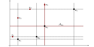
Figure 6. Illustration of the grid set ${\mathcal{G}}(\textbf{{u}}_{1},\ldots,\textbf{{u}}_{k})$, with $k=4$ points. The black squares represent the positions of $\textbf{{u}}_{1},\ldots,\textbf{{u}}_{4}$, and the set ${\mathcal{A}}_{\textbf{{u}}_{3}}$ is represented in a red solid line. The red dots represent the positions of $\textbf{{v}}_{1},\ldots,\textbf{{v}}_{4}$: here we have that $\textbf{{v}}_{1}\in{\mathcal{A}}_{\textbf{{u}}_{2}}$ ($\sigma(1)=2$), $\textbf{{v}}_{2}\in{\mathcal{A}}_{\textbf{{u}}_{1}}$ ($\sigma(2)=1$), $\textbf{{v}}_{3}\in{\mathcal{A}}_{\textbf{{u}}_{4}}$ ($\sigma(3)=4$) and $\textbf{{v}}_{4}\in{\mathcal{A}}_{\textbf{{u}}_{3}}$ ($\sigma(4)=3$).

Let us denote $\bar{S}_{k}$ the set of all permutations $\sigma$ of $\{1,\ldots,k\}$ that are admissible pairings of the $\textbf{{v}}_{i}$’s with $\textbf{{u}}_{j}$’s, in the sense that they are compatible with the condition $\textbf{{u}}_{1}\prec\cdots\prec\textbf{{u}}_{k}$ and $\textbf{{v}}_{1}\prec\cdots\prec\textbf{{v}}_{k}$. All together, we have

$$\|g_{k}\|_{\nu_{k}}^{2}=\!\!\idotsint\limits_{\begin{subarray}{c}{\boldsymbol{0}}\prec\textbf{{u}}_{1}\prec\cdots\prec\textbf{{u}}_{k}\prec{\boldsymbol{1}}\\ {\boldsymbol{0}}\prec\textbf{{v}}_{1}\prec\cdots\prec\textbf{{v}}_{k}\prec{\boldsymbol{1}}\end{subarray}}\!\!{\sf 1}_{\{\exists\sigma\in\bar{S}_{k}\,,\textbf{{v}}_{\sigma(i)}\in{\mathcal{A}}_{\textbf{{u}}_{i}}\forall i\}}g_{k}(\textbf{{u}}_{1},\ldots,\textbf{{u}}_{k})g_{k}(\textbf{{v}}_{1},\ldots,\textbf{{v}}_{k})\mathrm{d}\nu_{k}(\textbf{{u}}_{1},\ldots,\textbf{{u}}_{k},\textbf{{v}}_{1},\ldots,\textbf{{v}}_{k}).$$

Let us stress that $\bar{S}_{k}$ does not contain all permutations: indeed, we cannot have $\textbf{{u}}_{1}\prec\textbf{{u}}_{2}\prec\textbf{{u}}_{3}$ and $\textbf{{v}}_{1}\prec\textbf{{v}}_{2}\prec\textbf{{v}}_{3}$ with the following “alignment pattern”: $\textbf{{v}}_{3}\leftrightarrow\textbf{{u}}_{1}$, $\textbf{{v}}_{2}\leftrightarrow\textbf{{u}}_{2}$, $\textbf{{v}}_{1}\leftrightarrow\textbf{{u}}_{3}$. Hence, admissible permutations must avoid the pattern $(3\,2\,1)$. Since there are $C_{n}=\frac{1}{n+1}\binom{2n}{n}\leq 4^{n}$ such permutations (see e.g. [51] for a recent account on permutations avoiding patterns of length $3$), we get that

(4.16) $$|\bar{S}_{k}|\;\leq\;4^{k}\;.$$

Therefore, recalling that $g_{k}(\textbf{{u}})=\prod_{i=1}^{k+1}g(\textbf{{u}}_{i}-\textbf{{u}}_{i-1})$ with by convention $\textbf{{u}}_{0}={\boldsymbol{0}}$, $\textbf{{u}}_{k+1}={\boldsymbol{1}}$, the proof then consists in showing that, for any $\sigma\in\bar{S}_{k}$,

(4.17) $$\idotsint\limits_{\begin{subarray}{c}{\boldsymbol{0}}\prec\textbf{{u}}_{1}\prec\cdots\prec\textbf{{u}}_{k}\prec{\boldsymbol{1}}\\ {\boldsymbol{0}}\prec\textbf{{v}}_{1}\prec\cdots\prec\textbf{{v}}_{k}\prec{\boldsymbol{1}}\end{subarray}}\prod_{i=1}^{k+1}\Big{(}g(\textbf{{u}}_{\sigma(i)}-\textbf{{u}}_{\sigma(i)-1})g(\textbf{{v}}_{i}-\textbf{{v}}_{i-1}){\sf 1}_{\{\textbf{{v}}_{i}\in{\mathcal{A}}_{\textbf{{u}}_{\sigma(i)}}\}}\Big{)}\mathrm{d}\nu_{k}(\textbf{{u}}_{1},\ldots,\textbf{{u}}_{k},\textbf{{v}}_{1},\ldots,\textbf{{v}}_{k})\\[-15.0pt] \leq\frac{C^{k}}{\Gamma\big{(}k(\alpha-\frac{1}{2})\big{)}}\,.$$

This is a consequence of the following proposition.

Proposition 4.16.

There exists some (explicit) $C_{\alpha}>0$ such that for ${\boldsymbol{0}}\preccurlyeq\textbf{{u}}_{0}\prec\textbf{{u}}_{1}\preccurlyeq{\boldsymbol{1}}$, ${\boldsymbol{0}}\preccurlyeq\textbf{{v}}_{0}\prec\textbf{{v}}_{1}\preccurlyeq{\boldsymbol{1}}$ and $k\in\mathbb{N}\cup\{0\}$,

(4.18) $$\int_{[\textbf{{u}}_{0},\textbf{{u}}_{1}]\times[\textbf{{v}}_{0},\textbf{{v}}_{1}]}\|\textbf{{u}}-\textbf{{u}}_{0}\|^{k(\alpha-\frac{1}{2})}g(\textbf{{u}}-\textbf{{u}}_{0})g(\textbf{{v}}-\textbf{{v}}_{0})g(\textbf{{u}}_{1}-\textbf{{u}})g(\textbf{{v}}_{1}-\textbf{{v}})\mathrm{d}\nu_{\mathcal{M}}(\textbf{{u}},\textbf{{v}})$$

$$\hskip 85.35826pt\leq\;C_{\alpha}\,\widetilde{\Gamma}(k)\,\|\textbf{{u}}_{1}-\textbf{{u}}_{0}\|^{(k+1)(\alpha-\frac{1}{2})}g(\textbf{{u}}_{1}-\textbf{{u}}_{0})g(\textbf{{v}}_{1}-\textbf{{v}}_{0})\,,$$

where $\widetilde{\Gamma}(k):=\frac{\Gamma(k(\alpha-\frac{1}{2}))}{\Gamma((k+1)(\alpha-\frac{1}{2}))}$ if $k\in\mathbb{N}$, and $\widetilde{\Gamma}(0):=1$.

Applying Proposition 4.16 iteratively, we obtain (4.17), which concludes the proof. ∎

Proof of Proposition 4.16.

The way to estimate the integral in (4.18) depends on the respective locations of $\textbf{{u}}_{0},\textbf{{u}}_{1},\textbf{{v}}_{0},\textbf{{v}}_{1}$. We only treat the case $\textbf{{u}}_{0}^{(1)}<\textbf{{v}}^{(1)}_{0}<\textbf{{u}}^{(1)}_{1}<\textbf{{v}}^{(1)}_{1}$ and $\textbf{{v}}^{(2)}_{0}<\textbf{{u}}^{(2)}_{0}<\textbf{{v}}^{(2)}_{1}<\textbf{{u}}^{(2)}_{1}$, see Figure 7; other cases are analogous (or easier) and can be treated with similar techniques. We will actually estimate the integral in (4.18) restricted to $\textbf{{u}},\textbf{{v}}$ being on the same column, i.e. to $\textbf{{u}}^{(1)}=\textbf{{v}}^{(1)}$; the case where $\textbf{{u}},\textbf{{v}}$ are on the same line is similar.

We introduce the following notation, which will be used throughout the proof (we refer to Figure 7 for a graphical representation):

(4.19) $$x:=\textbf{{u}}^{(1)}-\textbf{{v}}_{0}^{(1)}=\textbf{{v}}^{(1)}-\textbf{{v}}_{0}^{(1)}\,, \quad y:=\textbf{{u}}^{(2)}-\textbf{{u}}_{0}^{(2)}\,, \qquad z:=\textbf{{v}}^{(2)}-\textbf{{v}}^{(2)}_{0}\,,$$

$$\overline{x}:=\textbf{{u}}^{(1)}_{1}-\textbf{{v}}^{(1)}_{0}\,, \quad\overline{y}:=\textbf{{u}}^{(2)}_{1}-\textbf{{u}}^{(2)}_{0}\,, \qquad\overline{z}:=\textbf{{v}}^{(2)}_{1}-\textbf{{v}}^{(2)}_{0}\,,$$

and also $a:=\textbf{{v}}^{(1)}_{0}-\textbf{{u}}^{(1)}_{0}$ and $b:=\textbf{{v}}^{(1)}_{1}-\textbf{{u}}^{(1)}_{1}$.

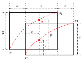
Figure 7. Illustration of the relative position of the points in the integral over $\textbf{{u}},\textbf{{v}}$ on the same column (in red). u (resp. v) is constrained to remain in a rectangle of size $\overline{x}\times\overline{y}$ (resp. $\overline{x}\times\overline{z}$), and their distances to $\textbf{{u}}_{0},\textbf{{u}}_{1},\textbf{{v}}_{0}$ and $\textbf{{v}}_{1}$ may be expressed in terms of $x,y,z$ and the constants $a,b,\overline{x},\overline{y}$ and $\overline{z}$.

With these notation, the integral in (4.18) restricted to $\textbf{{u}},\textbf{{v}}$ on the same column can be written as

$$\int_{0}^{\overline{x}}\int_{0}^{\overline{y}}\int_{0}^{\overline{z}}(x+y+a)^{k(\alpha-\frac{1}{2})}\big{[}(x+y+a)(x+z)(\overline{x}+\overline{y}-x-y)(\overline{x}+b+\overline{z}-x-z)\big{]}^{\alpha-2}\mathrm{d}x\,\mathrm{d}y\,\mathrm{d}z\,.$$

Using a change of variable $(x,s,t)=(x,x+y+a,x+z)$, we get

$$\int_{0}^{\overline{x}}\int_{x+a}^{x+\overline{y}+a}\int_{x}^{x+\overline{z}}s^{k(\alpha-\frac{1}{2})}\big{[}s\,t\,(\overline{s}-s)(\overline{t}-t)\big{]}^{\alpha-2}\,\mathrm{d}x\,\mathrm{d}s\,\mathrm{d}t$$

$$\qquad=\;\Big{(}\frac{\overline{s}}{2}\Big{)}^{k(\alpha-\frac{1}{2})}\Big{(}\frac{\overline{s}\,\overline{t}}{4}\Big{)}^{2\alpha-3}\int_{0}^{\overline{x}}\int_{2(x+a)/\overline{s}}^{2(x+\overline{y}+a)/\overline{s}}\int_{2x/\overline{t}}^{2(x+\overline{z})/\overline{t}}s^{k(\alpha-\frac{1}{2})}\big{[}s\,t\,(2-s)(2-t)\big{]}^{\alpha-2}\,\mathrm{d}x\,\mathrm{d}s\,\mathrm{d}t\,,$$

where we have set $\overline{s}:=\overline{x}+\overline{y}+a=\|\textbf{{u}}_{1}-\textbf{{u}}_{0}\|$, $\overline{t}:=\overline{x}+\overline{z}+b\;=\;\|\textbf{{v}}_{1}-\textbf{{v}}_{0}\|$, and then rescaled the last two integrals in $\overline{s}/2$, $\overline{t}/2$ respectively. Exchanging the integrals to first integrate with respect to $x$, this is equal to

(4.20) $$\Big{(}\frac{\overline{s}}{2}\Big{)}^{k(\alpha-\frac{1}{2})}\Big{(}\frac{\overline{s}\,\overline{t}}{4}\Big{)}^{2\alpha-3}\int_{0}^{2}\int_{0}^{2}s^{k(\alpha-\frac{1}{2})}\big{[}s\,t\,(2-s)(2-t)\big{]}^{\alpha-2}|A_{s,t}|\,\mathrm{d}s\,\mathrm{d}t\,,$$

where $A_{s,t}\subset[0,1]$ is defined by

(4.21) $$A_{s,t}\;:=\;\left\{x\in[0,\overline{x}]\;;\;x+a\in[\tfrac{s}{2}\overline{s}-\overline{y},\tfrac{s}{2}\overline{s}]\quad\text{and}\quad x\in[\tfrac{t}{2}\overline{t}-\overline{z},\tfrac{t}{2}\overline{t}]\right\}\,,$$

and $|A_{s,t}|$ denotes its Lebesgue measure. Therefore, the proof will be over once we show

(4.22) $$\int_{0}^{2}\int_{0}^{2}s^{k(\alpha-\frac{1}{2})}\big{[}s\,t\,(2-s)(2-t)\big{]}^{\alpha-2}|A_{s,t}|\,\mathrm{d}s\,\mathrm{d}t\;\leq\;C_{\alpha}\,2^{k(\alpha-\frac{1}{2})}\,\widetilde{\Gamma}(k)\,\Big{(}\frac{\overline{s}\,\overline{t}}{4}\Big{)}^{\frac{1}{2}}\,,$$

for some $C_{\alpha}>0$. Indeed, plugging (4.22) into (4.20), we get that the integral in (4.18) is bounded by

$$4^{\frac{5}{2}-2\alpha}C_{\alpha}\,\widetilde{\Gamma}(k)\,\bar{s}^{(k+1)(\alpha-\frac{1}{2})+(\alpha-2)}\,\bar{t}^{(\alpha-2)+(\alpha-\frac{1}{2})}\,,$$

which concludes the proof of (4.18) since $\overline{t}^{(\alpha-\frac{1}{2})}\leq 2^{\alpha-\frac{1}{2}}$ (recall $\textbf{{v}}_{1},\textbf{{v}}_{0}\in[{\boldsymbol{0}},{\boldsymbol{1}}]$).

Proof of (4.22). Let us first state an inequality which will prove useful henceforth:

(4.23) $$x\wedge y\;\leq\;\sqrt{(x\wedge y)(x\vee y)}\;=\;\sqrt{x\,y}\;,\qquad\forall\,x,y>0\,.$$

We split the l.h.s. of (4.22) into four integrals over the sets $I_{1}=\{s,t\leq 1\}$, $I_{2}=\{1\leq s,t\}$, $I_{3}=\{t\leq 1\leq s\}$ and $I_{4}=\{s\leq 1\leq t\}$ respectively, and we compute an upper bound for each term.

Integral over $I_{1}$. Since $A_{s,t}\subset[0,\frac{s}{2}\overline{s}]\cap[0,\frac{t}{2}\overline{t}]$, we have $|A_{s,t}|\leq(\tfrac{\overline{s}}{2}s)\wedge(\tfrac{\overline{t}}{2}t)\leq(\frac{\overline{s}\overline{t}}{4})^{1/2}(st)^{1/2}$ thanks to (4.23). Therefore, the integral over $I_{1}$ verifies

$$\int_{0}^{1}\int_{0}^{1}s^{k(\alpha-\frac{1}{2})}\big{[}s\,t\,(2-s)(2-t)\big{]}^{\alpha-2}|A_{s,t}|\,\mathrm{d}s\,\mathrm{d}t \leq\;\Big{(}\frac{\overline{s}\overline{t}}{4}\Big{)}^{\frac{1}{2}}\int_{0}^{1}s^{k(\alpha-\frac{1}{2})+\alpha-\frac{3}{2}}\,\mathrm{d}s\int_{0}^{1}t^{\alpha-\frac{3}{2}}\,\mathrm{d}t$$

$$=\frac{1}{\alpha-\frac{1}{2}}\frac{1}{(k+1)(\alpha-\frac{1}{2})}\Big{(}\frac{\overline{s}\overline{t}}{4}\Big{)}^{\frac{1}{2}}$$

where the last identity holds because $\alpha>1/2$ and $k\geq 0$. Then, we observe that there is $k_{\alpha}\in\mathbb{N}$ such that $\Gamma$ is increasing on $[k_{\alpha}(\alpha-\frac{1}{2}),\infty)$, hence for $k\geq k_{\alpha}$,

(4.24) $$\frac{1}{(k+1)(\alpha-\frac{1}{2})}\leq\frac{1}{k(\alpha-\frac{1}{2})}=\frac{\Gamma(k(\alpha-\frac{1}{2}))}{\Gamma(k(\alpha-\frac{1}{2})+1)}\;\leq\;\widetilde{\Gamma}(k)\;\leq\;2^{k(\alpha-\frac{1}{2})}\,\widetilde{\Gamma}(k)\;.$$

Fixing a suitable $C_{\alpha}>0$, this proves the upper bound (4.22) for the integral restricted on $I_{1}=\{s,t\leq 1\}$.

Integral over $I_{2}$. Recalling (4.21), we have $A_{s,t}\subset[\frac{s}{2}\overline{s}-\overline{y}-a,\overline{x}]\cap[\frac{t}{2}\overline{t}-\overline{z},\overline{x}]$, hence

$$|A_{s,t}|\;\leq\;\big{(}\overline{x}+\overline{y}+a-\tfrac{\overline{s}}{2}s\big{)}\wedge\big{(}\overline{x}+\overline{z}-\tfrac{\overline{t}}{2}t\big{)}\;\leq\;\big{(}\overline{s}(1-\tfrac{s}{2})\big{)}\wedge\big{(}\overline{t}(1-\tfrac{t}{2})\big{)}\;\leq\;\Big{(}\frac{\overline{s}\overline{t}}{4}\Big{)}^{\frac{1}{2}}\big{(}(2-s)(2-t)\big{)}^{\frac{1}{2}}\,,$$

where we used (4.23). Therefore,

$$\int_{1}^{2}\int_{1}^{2}s^{k(\alpha-\frac{1}{2})}\big{[}s\,t\,(2-s)(2-t)\big{]}^{\alpha-2}|A_{s,t}|\,\mathrm{d}s\,\mathrm{d}t \leq\Big{(}\frac{\overline{s}\overline{t}}{4}\Big{)}^{\frac{1}{2}}\int_{1}^{2}s^{k(\alpha-\frac{1}{2})-1}(2-s)^{\alpha-\frac{3}{2}}\,\mathrm{d}s\int_{1}^{2}(2-t)^{\alpha-\frac{3}{2}}\,\mathrm{d}t$$

(4.25) $$=\frac{1}{\alpha-\frac{1}{2}}\Big{(}\frac{\overline{s}\overline{t}}{4}\Big{)}^{\frac{1}{2}}\int_{1}^{2}s^{k(\alpha-\frac{1}{2})-1}(2-s)^{\alpha-\frac{3}{2}}\,\mathrm{d}s$$

where we also used that $s^{\alpha-1}\leq 1$ for $s\in[1,2]$ in the first inequality. For $k=0$ the integral above is finite, which proves (4.22); for $k\geq 1$, we recall that $\int_{0}^{1}x^{a-1}(1-x)^{b-1}\mathrm{d}x=\frac{\Gamma(a)\Gamma(b)}{\Gamma(a+b)}$, $a,b>0$, which yields (since $\alpha>1/2$)

(4.26) $$\int_{1}^{2}s^{k(\alpha-\frac{1}{2})-1}(2-s)^{\alpha-\frac{3}{2}}\,\mathrm{d}s\;\leq\;\int_{0}^{2}s^{k(\alpha-\frac{1}{2})-1}(2-s)^{\alpha-\frac{3}{2}}\,\mathrm{d}s\;\leq\;C_{\alpha}\,2^{k(\alpha-\frac{1}{2})}\,\frac{\Gamma(k(\alpha-\tfrac{1}{2}))\Gamma(\alpha-\frac{1}{2})}{\Gamma((k+1)(\alpha-\tfrac{1}{2}))}\,.$$

We conclude by recognizing the definition of $\widetilde{\Gamma}(k)$.

Integral over $I_{3}$. Similarly to the previous cases, we have $A_{s,t}\subset[\frac{s}{2}\overline{s}-\overline{y}-a,\overline{x}]\cap[0,\frac{t}{2}\overline{t}]$, so (4.23) implies

$$|A_{s,t}|\leq\big{(}\overline{s}(1-\tfrac{s}{2})\big{)}\wedge\big{(}\tfrac{t}{2}\overline{t}\big{)}\;\leq\;\Big{(}\frac{\overline{s}\overline{t}}{4}\Big{)}^{\frac{1}{2}}\big{(}(2-s)t\big{)}^{\frac{1}{2}}\,.$$

Thus,

$$\int_{1}^{2}\int_{0}^{1}s^{k(\alpha-\frac{1}{2})}\big{[}s\,t\,(2-s)(2-t)\big{]}^{\alpha-2}|A_{s,t}|\,\mathrm{d}s\,\mathrm{d}t\leq\Big{(}\frac{\overline{s}\overline{t}}{4}\Big{)}^{\frac{1}{2}}\int_{1}^{2}s^{k(\alpha-\frac{1}{2})-1}(2-s)^{\alpha-\frac{3}{2}}\,\mathrm{d}s\int_{0}^{1}t^{\alpha-\frac{3}{2}}\,\mathrm{d}t\,,$$

and a straightforward change of variable $t\to(2-t)$ yields the same upper bound as in (4.25)-(4.26).

Integral over $I_{4}$. With the same argument as before we have $|A_{s,t}|\leq(\tfrac{\overline{s}\overline{t}}{4})^{\frac{1}{2}}(s(2-t))^{\frac{1}{2}}$, so we get

$$\int_{0}^{1}\int_{1}^{2}s^{k(\alpha-\frac{1}{2})}\big{[}s\,t\,(2-s)(2-t)\big{]}^{\alpha-2}\lambda(A_{s,t})\,\mathrm{d}s\,\mathrm{d}t \leq\Big{(}\frac{\overline{s}\overline{t}}{4}\Big{)}^{\frac{1}{2}}\int_{0}^{1}s^{k(\alpha-\frac{1}{2})+\alpha-\frac{3}{2}}\,\mathrm{d}s\int_{1}^{2}(2-t)^{\alpha-\frac{3}{2}}\,\mathrm{d}t$$

$$=\frac{1}{\alpha-\frac{1}{2}}\frac{1}{(k+1)(\alpha-\frac{1}{2})}\Big{(}\frac{\overline{s}\overline{t}}{4}\Big{)}^{\frac{1}{2}}\;.$$

Then we conclude the proof as for the term $I_{1}$, with (4.24). ∎

5. Convergence of the polynomial chaos expansion

In this section we consider the polynomial expansion of the partition function. Similarly to Proposition 4.13 we focus on the constrained partition function (the cases of the conditioned or free partition function are analogous, recall Remark 4.15): similarly to (2.1), we have

(5.1) $$Z_{\lfloor n\textbf{{t}}\rfloor,h_{n}}^{\beta_{n},\omega,\mathrm{q}}=e^{\beta_{n}\omega_{\lfloor n\textbf{{t}}\rfloor}-\lambda(\beta_{n})+h_{n}}\sum_{k=0}^{\lfloor nt_{1}\rfloor\wedge\lfloor nt_{2}\rfloor}\sum_{{\boldsymbol{0}}=\textbf{{i}}_{0}\prec\textbf{{i}}_{1}\prec\ldots\prec\textbf{{i}}_{k+1}=\lfloor n\textbf{{t}}\rfloor}\prod_{l=1}^{k}(e^{h_{n}}\zeta_{\textbf{{i}}_{l}}+e^{h_{n}}-1)\,\prod_{l=1}^{k+1}u(\textbf{{i}}_{l}-\textbf{{i}}_{l-1})\,.$$

Let us highlight the different steps of the proof. First, we show that one can reduce to treating the case $h_{n}=0$, simply by expanding the product $\prod_{l=1}^{k}(e^{h_{n}}\zeta_{\textbf{{i}}_{l}}+e^{h_{n}}-1)$ and factorizing in the homogeneous partition function. Then, we show the $L^{2}$ convergence of the $k$-th term of the expansion to a (multivariate) integral against ${\mathcal{M}}$, for each $k\geq 1$ separately: this is the purpose of Proposition 5.1. To conclude the proof, we control the $L^{2}$ norm of each term of the expansion: we show that the $L^{2}$ norm of the $k$-th term is bounded by some constant $c_{k}$ uniformly in $n$, with $c_{k}$ summable—this is the content of Proposition 5.3.

Before starting the proof, let us recall the assumptions of Theorem 2.8 we work with in this section: we have $\alpha\in(\frac{1}{2},1)$, $\mathbb{P}\in\mathfrak{P}_{r}$ for some $r\in\mathbb{N}$, and the scaling relations (2.6) for $h_{n},\beta_{n}$. Recall also the definition (2.14) of $\psi:=\psi_{\textbf{{t}}}$, where we drop the index t to lighten notation—we work with a fixed t. Also, to lighten notation, from now on we write $n\textbf{{t}},nt_{1},nt_{2}$ omitting the integer part.

5.1. Reducing to the case $h_{n}=0$

Let us first explain how to reduce to the case $h_{n}=0$.

At the continuous level, note that expanding the product $\prod_{j=1}^{k}(\sigma_{r}\widehat{\beta}^{r}\,\mathrm{d}{\mathcal{M}}(\textbf{{s}}_{j})+\widehat{h}\,\mathrm{d}\textbf{{s}}_{j})$ in (2.13) and summing over points between indices where $\mathrm{d}{\mathcal{M}}(\textbf{{s}}_{j})$ appears, we get that the continuum partition function (2.13) can be rewritten as

$$\mathbf{Z}_{\textbf{{t}},\widehat{h}}^{\widehat{\beta},{\mathcal{M}},\mathrm{q}} =\sum_{\ell=0}^{+\infty}(\sigma_{r}\widehat{\beta}^{r})^{\ell}\idotsint\limits_{{\boldsymbol{0}}\prec\textbf{{s}}_{1}\prec\cdots\prec\textbf{{s}}_{\ell}\prec\textbf{{t}}}\ \prod_{j=1}^{\ell+1}\bigg{(}\sum_{k_{j}=0}^{+\infty}\widehat{h}^{k_{j}}\idotsint\limits_{\textbf{{s}}_{j-1}\prec\textbf{{s}}^{\prime}_{1}\prec\cdots\prec\textbf{{s}}^{\prime}_{k_{j}}\prec\textbf{{s}}_{j}}\prod_{i=1}^{k_{j}+1}\varphi(\textbf{{s}}^{\prime}_{i}-\textbf{{s}}^{\prime}_{i-1})\prod_{i=1}^{k_{j}}\mathrm{d}\textbf{{s}}^{\prime}_{i}\bigg{)}\prod_{j=1}^{\ell}\mathrm{d}{\mathcal{M}}(\textbf{{s}}_{j})$$

(5.2) $$=\sum_{\ell=0}^{+\infty}(\sigma_{r}\widehat{\beta}^{r})^{\ell}\idotsint\limits_{{\boldsymbol{0}}\prec\textbf{{s}}_{1}\prec\cdots\prec\textbf{{s}}_{\ell}\prec\textbf{{t}}}\psi^{(\widehat{h})}_{\textbf{{t}}}\big{(}\textbf{{s}}_{1},\ldots,\textbf{{s}}_{\ell}\big{)}\prod_{j=1}^{\ell}\mathrm{d}{\mathcal{M}}(\textbf{{s}}_{j})\,.$$

where, analogously to (2.14), we have defined

(5.3) $$\psi^{(\widehat{h})}_{\textbf{{t}}}\big{(}\textbf{{s}}_{1},\ldots,\textbf{{s}}_{k}\big{)}:={\sf 1}_{\{{\boldsymbol{0}}=:\textbf{{s}}_{0}\prec\textbf{{s}}_{1}\prec\cdots\prec\textbf{{s}}_{k}\prec\textbf{{s}}_{k+1}:=\textbf{{t}}\}}\prod_{j=1}^{k+1}\mathbf{Z}_{\textbf{{s}}_{j}-\textbf{{s}}_{j-1},\widehat{h}}\,,$$

recalling the definition of $\mathbf{Z}_{\textbf{{s}},\widehat{h}}$ in Proposition 2.3.

At the discrete level, analogously to what is done in (5.2), expanding the product $\prod_{l=1}^{k+1}(e^{h_{n}}\zeta_{\textbf{{i}}_{l}}+e^{h_{n}}-1)$ and rearranging the terms, we can rewrite (5.1) as

$$e^{-(\beta_{n}\omega_{n\textbf{{t}}}-\lambda(\beta_{n}))}Z_{\lfloor n\textbf{{t}}\rfloor,h_{n}}^{\beta_{n},\omega,\mathrm{q}}\\ =\sum_{\ell=0}^{\infty}\sum_{{\boldsymbol{0}}=\textbf{{i}}_{0}\prec\textbf{{i}}_{1}\prec\ldots\prec\textbf{{i}}_{\ell}\prec\textbf{{i}}_{\ell+1}=n\textbf{{t}}}\prod_{j=1}^{\ell}\zeta_{\textbf{{i}}_{j}}\prod_{j=1}^{\ell+1}e^{h_{n}}\bigg{(}\sum_{k_{j}=1}^{\infty}(e^{h_{n}}-1)^{k_{j}}\sum_{\textbf{{i}}_{j-1}=\textbf{{i}}^{\prime}_{0}\prec\textbf{{i}}^{\prime}_{1}\prec\ldots\prec\textbf{{i}}^{\prime}_{k_{j}}\prec\textbf{{i}}^{\prime}_{k_{j}+1}=\textbf{{i}}_{j}}\prod_{a=1}^{k_{j}}u(\textbf{{i}}_{a}-\textbf{{i}}_{a-1})\bigg{)}\\ =\sum_{\ell=0}^{\infty}\sum_{{\boldsymbol{0}}=\textbf{{j}}_{0}\prec\textbf{{j}}_{1}\prec\ldots\prec\textbf{{j}}_{\ell}\prec\textbf{{j}}_{\ell+1}=n\textbf{{t}}}\prod_{j=1}^{\ell}\zeta_{\textbf{{i}}_{j}}\prod_{j=1}^{\ell+1}Z_{\textbf{{i}}_{j}-\textbf{{i}}_{j-1},h_{n}}\,,$$

where we recognized the expansion of the homogeneous partition function $Z_{\textbf{{i}},h_{n}}$ to get the last identity, see (6.1).

Then, we can set $u^{(h_{n})}(\textbf{{i}}):=Z_{\textbf{{i}},h_{n}}$, and observe that thanks to Proposition 2.3 (which is proven in Section 6 by a standard Riemann-sum approximation) we have, for any $\textbf{{s}}\succ{\boldsymbol{0}}$,

$$\lim_{n\to\infty}n^{2-\alpha}L(n)u^{(h_{n})}(\lfloor n\textbf{{s}}\rfloor)=\mathbf{Z}_{\textbf{{s}},\widehat{h}}=:\varphi^{(\widehat{h})}(s)\,.$$

Note also that Lemma 6.1 which provides the uniform bound $u^{(h_{n})}(\textbf{{i}})\leq C_{\widehat{h}}L(\|\textbf{{i}}\|_{1})^{-1}\|\textbf{{i}}\|_{1}^{\alpha-2}$.

These are the two key properties that allow us to adapt the proof of Theorem 2.8, performed in the case $h_{n}\equiv 0$, to a general sequence $(h_{n})_{n\geq 1}$ (satisfying (2.6)). Indeed, we simply need to replace the renewal mass function $u(\cdot)$ with $u^{(h_{n})}(\cdot)$ and use Lemma 6.1 instead of $u(\textbf{{i}})\leq CL(\|\textbf{{i}}\|_{1})^{-1}\|\textbf{{i}}\|_{1}^{\alpha-2}$, which comes from [8, Thm. 4.1]. In the limit, the $k$-points correlation function $\psi(\textbf{{s}}_{1},\ldots,\textbf{{s}}_{k})=\prod_{i=1}^{k+1}\varphi(\textbf{{s}}_{i}-\textbf{{s}}_{i-1})$ for ${\boldsymbol{0}}\prec\textbf{{s}}_{0}\prec\textbf{{s}}_{1}\prec\cdots\prec\textbf{{s}}_{k+1}=\textbf{{t}}$ from (2.14) is simply replaced by $\psi^{(\widehat{h})}=\prod_{i=1}^{k}\varphi^{(\widehat{h})}(\textbf{{s}}_{i}-\textbf{{s}}_{i-1})$ defined in (5.3), as appears in (5.2).

5.2. Rewriting of the $k$-th term as a discrete integral

We now focus on the following expansion, for $h_{n}=0$:

$$n^{2-\alpha}L(n)Z_{n\textbf{{t}},h_{n}=0}^{\beta_{n},\omega,\mathrm{q}}=e^{\beta_{n}\omega_{n\textbf{{t}}}-\lambda(\beta_{n})}\sum_{k=0}^{\infty}\sum_{{\boldsymbol{0}}=\textbf{{i}}_{0}\prec\textbf{{i}}_{1}\prec\ldots\prec\textbf{{i}}_{k}\prec\textbf{{i}}_{k+1}=n\textbf{{t}}}n^{2-\alpha}L(n)\prod_{l=1}^{k}\zeta_{\textbf{{i}}_{l}}\prod_{l=1}^{k+1}u(\textbf{{i}}_{l}-\textbf{{i}}_{l-1})\,,$$

which leads us to define

(5.4) $$\widetilde{Z}_{n,k}:=\sum_{{\boldsymbol{0}}=\textbf{{i}}_{0}\prec\textbf{{i}}_{1}\prec\ldots\prec\textbf{{i}}_{k}\prec\textbf{{i}}_{k+1}=n\textbf{{t}}}n^{2-\alpha}L(n)\prod_{l=1}^{k}\zeta_{\textbf{{i}}_{l}}\prod_{l=1}^{k+1}u(\textbf{{i}}_{l}-\textbf{{i}}_{l-1})\,.$$

Note that the prefactor $e^{-(\beta_{n}\omega_{n\textbf{{t}}}-\lambda(\beta_{n}))}$ is irrelevant since it converges to 1 in $L^{2}$. The main idea is to rewrite the $k$-th term $\widetilde{Z}_{n,k}$ as some “integral” of a discrete approximation $\psi_{m}$ of $\psi$ against the product discrete field $\overline{M}_{n}^{\otimes k}$. Note that we use different indices $m,n$ for the approximation of the correlation function $\psi$ and for the approximation of the field ${\mathcal{M}}$: in the proof, the idea is to first let $n\to\infty$ and then $m\to\infty$.

Let us introduce some notation. For $m\in\mathbb{N}$, let $\Delta_{m}:=[{\boldsymbol{0}},\frac{1}{m}{\boldsymbol{1}})$ and ${\mathcal{D}}_{m}:=\frac{1}{m}\mathbb{Z}^{2}\cap[{\boldsymbol{0}},\textbf{{t}}]$. For $k,m,n\in\mathbb{N}$ and a function $g_{m}:[{\boldsymbol{0}},\textbf{{t}}]^{k}\to\mathbb{R}$ constant on each $\prod_{l=1}^{k}(\textbf{{u}}_{l}+\Delta_{m})$, $\textbf{{u}}_{1},\ldots,\textbf{{u}}_{k}\in{\mathcal{D}}_{m}$, we define the $k$-iterated “discrete integral” of $g_{m}$ against $\overline{M}_{n}$,

(5.5) $$g_{m}\overset{k}{\cdot}\overline{M}_{n}\;:=\;\sum_{\textbf{{u}}_{1},\ldots,\textbf{{u}}_{k}\in{\mathcal{D}}_{m}}g_{m}(\textbf{{u}}_{1},\ldots,\textbf{{u}}_{k})\hskip 1.0pt\prod_{l=1}^{k}\overline{M}_{n}\big{(}\textbf{{u}}_{l}-\tfrac{1}{n}{\boldsymbol{1}}+\Delta_{m}\big{)}\,,$$

where we refer to (3.3) for the definition of $\overline{M}_{n}$ and to (4.2) for the definition of increments of a field that appear in the last product. Note that the term $(-\tfrac{1}{n}{\boldsymbol{1}})$ is added to ensure that, if $n=m$ and $\frac{1}{n}\textbf{{i}}\in{\mathcal{D}}_{n}={\mathcal{D}}_{m}$, then we get $\overline{M}_{n}(\frac{1}{n}(\textbf{{i}}-{\boldsymbol{1}})+\Delta_{n})=\frac{1}{\sigma_{r}n^{3/2}\beta_{n}^{r}}\zeta_{\textbf{{i}},n}$, where we write $\zeta_{\textbf{{i}},n}:=\zeta_{\textbf{{i}}}=e^{\beta_{n}\omega_{\textbf{{i}}}-\lambda(\beta_{n})}-1$ for $\textbf{{i}}\in\mathbb{N}^{2}$ to keep track of the dependence on $n$.

Now, define

(5.6) $$\varphi_{m}(\textbf{{u}})\;:=\;m^{2-\alpha}L(m)\mathbf{P}\big{(}\lfloor m\textbf{{u}}\rfloor\in\boldsymbol{\tau}\big{)}\;,\qquad\textbf{{u}}\in[{\boldsymbol{0}},\textbf{{t}}]\;,$$

which is piecewise constant on each $(\textbf{{u}}+\Delta_{m})\cap[{\boldsymbol{0}},\textbf{{t}}]$, $\textbf{{u}}\in{\mathcal{D}}_{m}$. By Proposition 2.1 (from [72]), $\varphi_{m}$ converges simply to $\varphi$ as $m\to\infty$. With this at hand we define the piecewise constant approximation $\psi_{m}$ of $\psi$ by replacing $\varphi$ with $\varphi_{m}$ in its definition (2.14):

$$\psi_{m}(\textbf{{u}}_{1},\ldots,\textbf{{u}}_{k})=\varphi_{m}(\textbf{{u}}_{1})\,\varphi_{m}(\textbf{{u}}_{2}-\textbf{{u}}_{1})\,\cdots\,\varphi_{m}(\textbf{{t}}-\textbf{{u}}_{k}){\sf 1}_{\{{\boldsymbol{0}}\prec\textbf{{u}}_{1}\prec\cdots\prec\textbf{{u}}_{k}\prec\textbf{{t}}\}}\,.$$

With this notation, we can rewrite the $k$-th term $\widetilde{Z}_{n,k}$, see (5.4), as

(5.7) $$\widetilde{Z}_{n,k}=\bigg{(}\frac{\sigma_{r}n^{3/2}\beta_{n}^{r}}{n^{2-\alpha}L(n)}\bigg{)}^{k}\,\psi_{n}\overset{k}{\cdot}\overline{M}_{n}\;.$$

One of our main goals is to prove the following.

Proposition 5.1.

Let $k\geq 1$. Under the assumptions of Theorem 2.7, one has

$$\psi_{n}\overset{k}{\cdot}\overline{M}_{n}\quad\xrightarrow[n\to\infty]{(d)}\quad\psi\overset{k}{\diamond}{\mathcal{M}}\;.$$

This convergence holds in $L^{2}(\widehat{\mathbb{P}})$ on a convenient probability space $(\widehat{\Omega},\widehat{\mathcal{F}},\widehat{\mathbb{P}})$.

Recall from Proposition 4.13 that the stochastic integral $\psi\overset{k}{\diamond}{\mathcal{M}}$ is well defined.

Remark 5.2.

The “integral” $\psi_{n}\overset{k}{\cdot}\overline{M}_{n}$ that we introduced does not fall under the definition from Theorem 4.8. Even though one could define the covariance measure of $\overline{M}_{n}^{\otimes k}$ with a collection of Dirac masses, one cannot use a direct argument (such as dominated convergence) to get that $\psi_{n}\overset{k}{\diamond}\overline{M}_{n}^{\otimes k}$ converges towards $\psi\overset{k}{\diamond}{\mathcal{M}}$. Nonetheless, the development of such arguments would be an interesting expansion of our results towards a general methodology to study the influence of (correlated) disorder on physical systems.

5.3. Proof of Proposition 5.1

Recall from Claim 3.5 that, up to a change of probability space, we may assume that $(\overline{M}_{n})_{n\geq 1}$ converges $\mathbb{P}$-a.s. to $\overline{\mathcal{M}}$ and that all pointwise convergences hold in $L^{p}(\mathbb{P})$ for $p\geq 1$ (we do not change notation for simplicity’s sake). Hence we simply need to prove the $L^{2}(\mathbb{P})$ convergence on that probability space.

In order to deal with the fact that $\varphi$ blows up around ${\boldsymbol{0}}$, let us introduce a truncated version of $\varphi_{m},\psi_{m},\varphi,\psi$. For $\delta\geq 0$, let $\varphi_{m}^{\delta}(\textbf{{u}}):=\varphi_{m}(\textbf{{u}}){\sf 1}_{\{\|\textbf{{u}}\|\geq\delta\}}$ (note that $\varphi_{m}^{0}=\varphi_{m}$)and

$$\psi_{m}^{\delta}(\textbf{{u}}_{1},\ldots,\textbf{{u}}_{k}):=\varphi_{m}^{\delta}(\textbf{{u}}_{1})\,\varphi_{m}^{\delta}(\textbf{{u}}_{2}-\textbf{{u}}_{1})\,\cdots\,\varphi_{m}^{\delta}(\textbf{{t}}-\textbf{{u}}_{k}){\sf 1}_{\{{\boldsymbol{0}}\prec\textbf{{u}}_{1}\prec\cdots\prec\textbf{{u}}_{k}\prec\textbf{{t}}\}}\,.$$

We define similarly $\varphi^{\delta}(\textbf{{u}}):=\varphi(\textbf{{u}}){\sf 1}_{\{\|\textbf{{u}}\|\geq\delta\}}$ and $\psi^{\delta}$.

We write for $n\geq m$, $\delta>0$,

(5.8) $$\|\psi_{n}\overset{k}{\cdot}\overline{M}_{n}-\psi\overset{k}{\diamond}{\mathcal{M}}\|_{L^{2}}\;\leq\;I_{1}+I_{2}+I_{3}+I_{4}+I_{5}\;,$$

where

(5.9) $$\begin{array}[]{llll}I_{1}\;:=&\|\psi_{n}\overset{k}{\cdot}\overline{M}_{n}-\psi_{n}^{\delta}\overset{k}{\cdot}\overline{M}_{n}\|_{L^{2}}\,,&I_{2}\;:=&\|\psi_{n}^{\delta}\overset{k}{\cdot}\overline{M}_{n}-\psi_{m}^{\delta}\overset{k}{\cdot}\overline{M}_{n}\|_{L^{2}}\,,\vskip 3.0pt plus 1.0pt minus 1.0pt\\ I_{3}\;:=&\|\psi_{m}^{\delta}\overset{k}{\cdot}\overline{M}_{n}-\psi_{m}^{\delta}\overset{k}{\diamond}{\mathcal{M}}\|_{L^{2}}\,,&I_{4}\;:=&\|\psi_{m}^{\delta}\overset{k}{\diamond}{\mathcal{M}}-\psi^{\delta}\overset{k}{\diamond}{\mathcal{M}}\|_{L^{2}}\,,\vskip 3.0pt plus 1.0pt minus 1.0pt\\ I_{5}\;:=&\|\psi^{\delta}\overset{k}{\diamond}{\mathcal{M}}-\psi\overset{k}{\diamond}{\mathcal{M}}\|_{L^{2}}\,.&&\end{array}$$

We now need to control each term separately. We show that we can fix $\delta$ sufficiently small so that the terms $I_{1}$ and $I_{5}$ are small, uniformly in $n$ for $I_{1}$. Then, for a fixed $\delta$, we show that $I_{2},I_{4}$ can be made arbitrarily small by choosing $m$ large, uniformly in $n\geq m$ for $I_{2}$. It then remains to see that, for any fixed $m$ and $\delta$, $I_{3}$ vanishes as $n\to\infty$.

5.3.1. Term $I_{5}$

First of all, notice that we have $\lim_{\delta\to 0}\psi^{\delta}=\psi$, so by Proposition 4.13, the isometry property (4.8) and dominated (or monotone) convergence, we get that we can chose $\delta$ sufficiently small to make $I_{5}$ arbitrarily small.

5.3.2. Term $I_{1}$

We use the following key result, which shows that $I_{1}$ is arbitrarily small for small $\delta$, uniformly in $n$ large. Its proof is postponed to Section 5.5 below; it can be viewed as the core of the proof, and contains some of the most technical part of the paper. As a first part, we also include a bound on the $L^{2}$ norm of the discrete integral for the non-truncated $\psi_{n}$: this part is the discrete analogue of Proposition 4.13 and will prove useful later.

Proposition 5.3.

$(i)$ There exist constants $C,c>0$ and some $n_{0}\geq 1$ such that for any $k\in\mathbb{N}$, $n\geq n_{0}$, one has

(5.10) $$\|\psi_{n}\overset{k}{\cdot}\overline{M}_{n}\|_{L^{2}}^{2}\;\leq\;\frac{C^{k}}{\Gamma(k(\alpha-\frac{1}{2}))}+C^{k}\beta_{n}^{ck}\;.$$

$(ii)$ For every $k\in\mathbb{N}$, we have

(5.11) $$\lim_{\delta\downarrow 0}\limsup_{n\to\infty}\|\psi_{n}\overset{k}{\cdot}\overline{M}_{n}-\psi_{n}^{\delta}\overset{k}{\cdot}\overline{M}_{n}\|_{L^{2}}^{2}=0\;.$$

5.3.3. Term $I_{4}$

It is already clear that $\lim_{m\to\infty}I_{4}=0$: this follows from the fact that $\psi_{m}^{\delta}(\textbf{{u}})\to\psi^{\delta}(\textbf{{u}})$ as $m\to\infty$ for all $\textbf{{u}}\in[{\boldsymbol{0}},\textbf{{t}}]^{k}$, together with Proposition 4.13 and dominated convergence.

5.3.4. Term $I_{2}$

Let us show that the convergence $\lim_{m\to\infty}\psi_{m}^{\delta}=\psi^{\delta}$ actually holds for the $\|\cdot\|_{\infty}$ norm on $[{\boldsymbol{0}},\textbf{{t}}]^{k}$. First, the convergence $\lim_{m\to\infty}\varphi_{m}(\textbf{{u}})=\varphi(\textbf{{u}})$, $m\to\infty$ holds uniformly in $\textbf{{u}}\in[{\boldsymbol{0}},\textbf{{t}}]\setminus[0,\delta)^{2}$ for $\delta>0$ (see [72]). We therefore get that for $\delta>0$ fixed, $\lim_{m\to\infty}\|\varphi_{m}^{\delta}-\varphi^{\delta}\|_{\infty}=0$. Now, let $\textbf{{u}}:=(\textbf{{u}}_{1},\ldots,\textbf{{u}}_{k})$ with ${\boldsymbol{0}}=:\textbf{{u}}_{0}\preccurlyeq\textbf{{u}}_{1}\prec\ldots\prec\textbf{{u}}_{k}\preccurlyeq\textbf{{u}}_{k+1}:=\textbf{{t}}$. Then, by the simple fact (proven e.g. by recurrence) that

(5.12) $$\bigg{|}\prod_{i=1}^{k}a_{i}-\prod_{i=1}^{k}b_{i}\bigg{|}\leq\Big{(}\max_{1\leq i\leq k}\{|a_{i}|,|b_{i}|\}\Big{)}^{k-1}\sum_{i=1}^{k}|a_{i}-b_{i}|\,,$$

we get that

$$\bigg{|}\prod_{l=1}^{k+1}\varphi_{m}^{\delta}(\textbf{{u}}_{l}-\textbf{{u}}_{l-1})-\prod_{l=1}^{k+1}\varphi^{\delta}(\textbf{{u}}_{l}-\textbf{{u}}_{l-1})\bigg{|}\leq\;(k+1)\Big{(}\sup_{[{\boldsymbol{0}},\textbf{{t}}]\setminus[0,\delta)^{2}}(|\varphi_{m}(\textbf{{u}})|+|\varphi(\textbf{{u}})|)\Big{)}^{k}\;\big{\|}\varphi_{m}^{\delta}-\varphi^{\delta}\big{\|}_{\infty}\,.$$

Since, $|\varphi_{m}(\textbf{{u}})|,|\varphi(\textbf{{u}})|$ are bounded by a constant $C_{\delta}$ uniformly for $\|\textbf{{u}}\|\geq\delta$, this indeed shows that $\lim_{m\to\infty}\|\psi_{m}^{\delta}-\psi^{\delta}\|_{\infty}=0$.

Let us now prove that we can choose $m_{1}\in\mathbb{N}$ to make $I_{2}$ arbitrarily small uniformly in $n\geq m\geq m_{1}$. Notice that for $n\geq m$ and $\textbf{{u}}\in{\mathcal{D}}_{p}$, $p\in\{n,m\}$, we may rewrite

$$\overline{M}_{n}(\textbf{{u}}-\tfrac{1}{n}+\Delta_{p})\;=\;\sum_{{\boldsymbol{w}}\in(\textbf{{u}}+\Delta_{p})\cap{\mathcal{D}}_{nm}}\overline{M}_{n}({\boldsymbol{w}}-\tfrac{1}{n}+\Delta_{nm})\;,$$

which gives, with the definition (5.5),

(5.13) $$\psi^{\delta}_{m}\overset{k}{\cdot}\overline{M}_{n}-\psi^{\delta}_{n}\overset{k}{\cdot}\overline{M}_{n}\;=\;\sum_{{\boldsymbol{w}}\in({\mathcal{D}}_{nm})^{k}}\big{(}\psi^{\delta}_{m}({\boldsymbol{w}})-\psi^{\delta}_{n}({\boldsymbol{w}})\big{)}\prod_{l=1}^{k}\overline{M}_{n}({\boldsymbol{w}}_{l}-\tfrac{1}{n}+\Delta_{nm})\;.$$

Therefore, recalling that the correlations of the field $\overline{M}_{n}$ are non-negative, we have

$$\|\psi^{\delta}_{m}\overset{k}{\cdot}\overline{M}_{n}-\psi^{\delta}_{n}\overset{k}{\cdot}\overline{M}_{n}\|_{L^{2}}^{2} \leq\,\big{(}\|\psi_{m}^{\delta}-\psi_{n}^{\delta}\|_{\infty}\big{)}^{2}\!\!\sum_{{\boldsymbol{w}}\in({\mathcal{D}}_{nm})^{2k}}\!\mathbb{E}\Big{[}\prod_{l=1}^{2k}\overline{M}_{n}({\boldsymbol{w}}_{l}-\tfrac{1}{n}+\Delta_{nm})\Big{]}$$

$$\leq\,\big{(}\|\psi_{m}^{\delta}-\psi_{n}^{\delta}\|_{\infty}\big{)}^{2}\hskip 1.0pt\mathbb{E}\big{[}\overline{M}_{n}([{\boldsymbol{0}},\textbf{{t}}))^{2k}\big{]}\;=\;\big{(}\|\psi_{m}^{\delta}-\psi_{n}^{\delta}\|_{\infty}\big{)}^{2}\hskip 1.0pt\mathbb{E}\big{[}\overline{M}_{n}(\textbf{{t}})^{2k}\big{]}\;.$$

Recall that $(\mathbb{E}[\overline{M}_{n}(\textbf{{t}})^{2k}])_{n\geq 1}$ converges, so it is bounded. Thus, we conclude the proof by choosing $m_{1}\in\mathbb{N}$ such that, for $n\geq m\geq m_{1}$, $\|\psi_{m}^{\delta}-\psi_{n}^{\delta}\|_{\infty}$ is sufficiently small.

5.3.5. Term $I_{3}$

Let $m\in\mathbb{N}$ be fixed and $\delta\geq 0$ (we allow $\delta=0$). Since $\psi_{m}^{\delta}$ (or $\psi^{0}_{m}=\psi_{m}$) is constant on each $\prod_{l=1}^{k}(\frac{1}{m}\textbf{{i}}_{l}+\Delta_{m})$, $\textbf{{i}}_{1},\ldots,\textbf{{i}}_{k}\in\mathbb{N}_{0}^{2}$, there exists a family $\{a_{{\boldsymbol{w}}}\in\mathbb{R};{\boldsymbol{w}}=({\boldsymbol{w}}_{1},\ldots,{\boldsymbol{w}}_{k})\in({\mathcal{D}}_{m})^{k}\}$ such that for $(\textbf{{u}}_{1},\ldots,\textbf{{u}}_{k})\in[{\boldsymbol{0}},\textbf{{t}})^{k}$,

(5.14) $$\psi_{m}^{\delta}(\textbf{{u}}_{1},\ldots,\textbf{{u}}_{k})\;=\;\sum_{{\boldsymbol{w}}\in({\mathcal{D}}_{m})^{k}}a_{{\boldsymbol{w}}}\prod_{l=1}^{k}{\sf 1}_{[{\boldsymbol{0}},{\boldsymbol{w}}_{l})}(\textbf{{u}}_{l})\;.$$

Thus, starting from the definition (5.5), we get

(5.15) $$\psi_{m}^{\delta}\overset{k}{\cdot}\overline{M}_{n} =\;\sum_{\textbf{{u}}\in({\mathcal{D}}_{m})^{k}}\bigg{(}\sum_{{\boldsymbol{w}}\in({\mathcal{D}}_{m})^{k}}a_{\boldsymbol{w}}\prod_{l=1}^{k}{\sf 1}_{[{\boldsymbol{0}},{\boldsymbol{w}}_{l})}(\textbf{{u}}_{l})\bigg{)}\prod_{l=1}^{k}\overline{M}_{n}\big{(}\textbf{{u}}_{l}-\tfrac{1}{n}{\boldsymbol{1}}+\Delta_{m}\big{)}$$

$$=\;\sum_{{\boldsymbol{w}}\in({\mathcal{D}}_{m})^{k}}a_{\boldsymbol{w}}\sum_{\begin{subarray}{c}\textbf{{u}}\in({\mathcal{D}}_{m})^{k}\\ \textbf{{u}}\in\prod_{l=1}^{k}[{\boldsymbol{0}},{\boldsymbol{w}}_{l})\end{subarray}}\prod_{l=1}^{k}\overline{M}_{n}\big{(}\textbf{{u}}_{l}-\tfrac{1}{n}{\boldsymbol{1}}+\Delta_{m}\big{)}=\;\sum_{{\boldsymbol{w}}\in({\mathcal{D}}_{m})^{k}}a_{\boldsymbol{w}}\hskip 1.0pt\prod_{l=1}^{k}\hskip 1.0pt\overline{M}_{n}({\boldsymbol{w}}_{l}-\tfrac{1}{n}{\boldsymbol{1}})\;.$$

Recalling the definition of the integral $\overset{k}{\diamond}$, we have $(\prod_{l=1}^{k}{\sf 1}_{[{\boldsymbol{0}},{\boldsymbol{w}}_{l})})\overset{k}{\diamond}{\mathcal{M}}=\prod_{l=1}^{k}{\mathcal{M}}({\boldsymbol{w}}_{l})$. Hence we may also write with a similar computation

(5.16) $$\psi_{m}^{\delta}\overset{k}{\diamond}{\mathcal{M}}\;=\;\sum_{{\boldsymbol{w}}\in({\mathcal{D}}_{m})^{k}}a_{\boldsymbol{w}}\hskip 1.0pt\prod_{l=1}^{k}\hskip 1.0pt{\mathcal{M}}({\boldsymbol{w}}_{l})\;.$$

Using Proposition 3.2, it is clear that for fixed $\delta>0,m\in\mathbb{N}$ we have the convergence

(5.17) $$\sum_{{\boldsymbol{w}}\in({\mathcal{D}}_{m})^{k}}a_{\boldsymbol{w}}\hskip 1.0pt\prod_{l=1}^{k}\hskip 1.0pt\overline{M}_{n}({\boldsymbol{w}}_{l})\,\;\;\xrightarrow[n\to\infty]{L^{2}}\,\;\;\sum_{{\boldsymbol{w}}\in({\mathcal{D}}_{m})^{k}}a_{\boldsymbol{w}}\hskip 1.0pt\prod_{l=1}^{k}\hskip 1.0pt{\mathcal{M}}({\boldsymbol{w}}_{l})\,.$$

It remains to replace $\overline{M}_{n}({\boldsymbol{w}}_{l}-\tfrac{1}{n}{\boldsymbol{1}})$ with $\overline{M}_{n}({\boldsymbol{w}}_{l})$ in (5.15). For ${\boldsymbol{w}}_{1},\ldots,{\boldsymbol{w}}_{k}\in[{\boldsymbol{0}},\textbf{{t}})$, we have

$$\Big{\|}\prod_{l=1}^{k}\overline{M}_{n}({\boldsymbol{w}}_{l})-\prod_{l=1}^{k}\overline{M}_{n}({\boldsymbol{w}}_{l}-\tfrac{1}{n}{\boldsymbol{1}})\Big{\|}_{L^{2}}$$

$$\quad\leq\;\sum_{l=1}^{k}\Big{\|}\big{(}\overline{M}_{n}({\boldsymbol{w}}_{l})-\overline{M}_{n}({\boldsymbol{w}}_{l}-\tfrac{1}{n}{\boldsymbol{1}})\big{)}\prod_{j=1}^{l-1}\overline{M}_{n}({\boldsymbol{w}}_{l})\prod_{j=l+1}^{k}\overline{M}_{n}({\boldsymbol{w}}_{l}-\tfrac{1}{n}{\boldsymbol{1}})\Big{\|}_{L^{2}}$$

$$\quad\leq\;\sum_{l=1}^{k}\Bigg{(}\Big{\|}\overline{M}_{n}({\boldsymbol{w}}_{l})-\overline{M}_{n}({\boldsymbol{w}}_{l}-\tfrac{1}{n}{\boldsymbol{1}})\Big{\|}_{L^{2k}}\prod_{j=1}^{l-1}\Big{\|}\overline{M}_{n}({\boldsymbol{w}}_{l})\Big{\|}_{L^{2k}}\prod_{j=l+1}^{k}\Big{\|}\overline{M}_{n}({\boldsymbol{w}}_{l}-\tfrac{1}{n}{\boldsymbol{1}})\Big{\|}_{L^{2k}}\Bigg{)}\;,$$

where we used Hölder’s inequality. In each term of the sum, the $k-1$ last factors are all uniformly bounded by $\|\overline{M}_{n}(\textbf{{t}})\|_{L^{2k}}\leq C\|{\mathcal{M}}(\textbf{{t}})\|_{L^{2k}}<\infty$ (recall Claim 3.5). Then, the first factor goes to 0, thanks to Lemma 3.4, which proves that $\|\prod_{l=1}^{k}\overline{M}_{n}({\boldsymbol{w}}_{l})-\prod_{l=1}^{k}\overline{M}_{n}({\boldsymbol{w}}_{l}-\tfrac{1}{n}{\boldsymbol{1}})\|_{L^{2}}$ goes to $0$ as $n\to\infty$. Recollecting (5.15–5.17), this concludes the proof that $\lim_{n\to\infty}I_{3}=0$. Note that all the proof was also valid in the case $\delta=0$, so we also have that $\lim_{n\to\infty}\|\psi_{m}\overset{k}{\cdot}\overline{M}_{n}-\psi_{m}\overset{k}{\diamond}{\mathcal{M}}\|_{L^{2}}=0$.∎

5.4. Conclusion of the proof of Theorem 2.8

With the help of Proposition 5.1 and thanks to the first item of Proposition 5.3, we are able to conclude the proof of Theorem 2.8.

Indeed, in view of (5.7) and using the fact that $\lim_{n\to\infty}\frac{\beta_{n}^{r}}{n^{\frac{1}{2}-\alpha}L(n)}=\widehat{\beta}$ by (2.6), Proposition 5.1 shows that, for any fixed $k$,

$$\widetilde{Z}_{n,k}\xrightarrow[n\to\infty]{L^{2}}(\sigma_{r}\widehat{\beta})^{k}\,\psi\overset{k}{\diamond}{\mathcal{M}}=\idotsint\limits_{{\boldsymbol{0}}\prec\textbf{{s}}_{1}\prec\cdots\prec\textbf{{s}}_{k}\prec\textbf{{t}}}\psi_{\textbf{{t}}}\big{(}\textbf{{s}}_{1},\ldots,\textbf{{s}}_{k}\big{)}\prod_{j=1}^{k}\sigma_{r}\widehat{\beta}^{r}\,\mathrm{d}{\mathcal{M}}(\textbf{{s}}_{j})\,.$$

Then, item (i) of Proposition 5.3 shows that there is a constant $C>0$ and some $n_{0}\geq 0$ such that, for all $k\in\mathbb{N}$ and $n\geq n_{0}$,

$$\|\widetilde{Z}_{n,k}\|_{L^{2}}\leq\frac{C^{k}}{\Gamma(k(\alpha-\frac{1}{2}))^{1/2}}+(C\beta_{n}^{c/2})^{k}\leq\frac{C^{k}}{\Gamma(k(\alpha-\frac{1}{2}))^{1/2}}+2^{-k}\,.$$

Hence, we have the following bound on the $L^{2}$ norm of rest of the series, valid uniformly for $n\geq n_{0}$:

$$\Big{\|}\sum_{k\geq k_{0}}\widetilde{Z}_{n,k}\Big{\|}_{L^{2}}\leq\sum_{k\geq k_{0}}\|\widetilde{Z}_{n,k}\|_{L^{2}}\leq\sum_{k\geq k_{0}}\Big{(}\frac{C^{k}}{\Gamma(k(\alpha-\frac{1}{2}))^{1/2}}+2^{-k}\Big{)}\,,$$

which can be made arbitrarily small by choosing $k_{0}$ large. Hence, fixing $k_{0}>0$, letting $n\to\infty$ and then $k_{0}\to\infty$, we get that

$$\sum_{k=0}^{\infty}\widetilde{Z}_{n,k}\xrightarrow[n\to\infty]{L^{2}}\sum_{k=0}^{\infty}(\sigma_{r}\widehat{\beta})^{k}\,\psi\overset{k}{\diamond}{\mathcal{M}}=\mathbf{Z}_{\textbf{{t}},\widehat{h}=0}^{\widehat{\beta},{\mathcal{M}},\mathrm{q}}\,,$$

using also Corollary 4.14 to ensure that the r.h.s. is well-defined.∎

5.5. Proof of Proposition 5.3

The only thing that remains to be proven is now Proposition 5.3. We start with the proof of the first item and then we built on that proof to deal with the second item.

5.5.1. Proof of item (i) of Proposition 5.3

Notice that from (5.7), $\|\psi_{n}\overset{k}{\cdot}\overline{M}_{n}\|_{L^{2}}\leq C^{k}\|\widetilde{Z}_{n,k}\|_{L^{2}}$. We therefore need to control the $L^{2}$ norm of $\widetilde{Z}_{n,k}$ defined in (5.4), that can be written more compactly as

(5.18) $$\widetilde{Z}_{n,k}=n^{2-\alpha}L(n)\sum_{\textbf{{I}}\in{\mathcal{I}}_{k}}u_{n}(\textbf{{I}})\prod_{\textbf{{i}}\in\textbf{{I}}}\zeta_{\textbf{{i}}}\,,$$

where we have denoted

$$\mathcal{I}_{k}=\mathcal{I}_{k}(\textbf{{t}})=\Big{\{}\textbf{{I}}=(\textbf{{i}}_{1},\ldots,\textbf{{i}}_{k}),{\boldsymbol{0}}=:\textbf{{i}}_{0}\prec\textbf{{i}}_{1}\prec\cdots\prec\textbf{{i}}_{k}\prec n\textbf{{t}}=:\textbf{{i}}_{k+1}\Big{\}}$$

the set of increasing subsets of $\llbracket{\boldsymbol{1}},n\textbf{{t}}\rrbracket$ with cardinality $k$, and defined $u_{n}(\textbf{{I}}):=\prod_{l=1}^{k+1}u(\textbf{{i}}_{l}-\textbf{{i}}_{l-1})$ (with by convention $bi_{0}={\boldsymbol{0}}$, $\textbf{{i}}_{k+1}=n\textbf{{t}}$). With these notation, we need to control

(5.19) $$\|\widetilde{Z}_{n,k}\|_{L^{2}}^{2}=(n^{2-\alpha}L(n))^{2}\sum_{\textbf{{I}},\textbf{{J}}\in{\mathcal{I}}_{k}}u_{n}(\textbf{{I}})u_{n}(\textbf{{J}})\mathbb{E}\Big{[}\prod_{\textbf{{i}}\in\textbf{{I}},\textbf{{j}}\in\textbf{{J}}}\zeta_{\textbf{{i}}}\zeta_{\textbf{{j}}}\Big{]}\,.$$

Step 1. Controlling the correlation term

Since the indices in $\textbf{{I}},\textbf{{J}}$ are increasing, the set $\textbf{{I}}\cup\textbf{{J}}$ can be uniquely partitioned (as done in [56, Prop. 3.4]) into disjoint sets

(5.20) $$\boldsymbol{\iota}\cup\boldsymbol{\nu}\cup\bigcup_{m\in\mathbb{N}}\boldsymbol{\sigma}_{m}\,,$$

where:

• $\boldsymbol{\iota}$ is the set of isolated points, i.e. indices $\textbf{{i}}\in\textbf{{I}}$ (resp. in J) such that $\textbf{{j}}\not\leftrightarrow\textbf{{i}}$ for any $\textbf{{j}}\in\textbf{{J}}$ (resp. in I);

• $\boldsymbol{\nu}$ is the set of intersection points, i.e. indices that are both in I and J;

• $\sigma_{m}$ are chains of indices, i.e. indices $\textbf{{i}}_{1},\ldots,\textbf{{i}}_{p}$ (necessarily alternating between I and J) such that $\textbf{{i}}_{l+1}\leftrightarrow\textbf{{i}}_{l}$ for all $1\leq l\leq p-1$ and such that any other index in $\textbf{{I}}\cup\textbf{{J}}$ is not aligned with any of the $\textbf{{i}}_{l}$; the integer $p\geq 2$ is called the length of the chain.

By independence of the $\zeta_{\textbf{{i}}}$ for non-aligned sets, we get that

$$\mathbb{E}\Big{[}\prod_{\textbf{{i}}\in I,\textbf{{j}}\in J}\zeta_{\textbf{{i}}}\zeta_{\textbf{{j}}}\Big{]} =\mathbb{E}[\zeta_{{\boldsymbol{1}}}^{2}]^{|\boldsymbol{\nu}|}\mathbb{E}[\zeta_{{\boldsymbol{1}}}]^{|\boldsymbol{\iota}|}\prod_{m\in\mathbb{N}}\mathbb{E}\Big{[}\prod_{\textbf{{i}}\in\boldsymbol{\sigma}_{m}}\zeta_{\textbf{{i}}}\Big{]}$$

For fixed $\textbf{{I}},\textbf{{J}}$, let us denote $N_{0}(\textbf{{I}},\textbf{{J}})=|\boldsymbol{\iota}|$ the number of isolated points, $N_{1}(\textbf{{I}},\textbf{{J}})=|\boldsymbol{\nu}|$ the number of intersection points and $N_{p}(\textbf{{I}},\textbf{{J}})=|\{m,|\boldsymbol{\sigma}_{m}|=p\}|$ the number of chains of length $p$. The correlation is equal to $0$ when $N_{0}(\textbf{{I}},\textbf{{J}})\geq 1$, and in the case $N_{0}(\textbf{{I}},\textbf{{J}})=0$ we get, thanks to Lemma 3.1-(3.8),

(5.21) $$\mathbb{E}\Big{[}\prod_{\textbf{{i}}\in\textbf{{I}},\textbf{{j}}\in\textbf{{J}}}\zeta_{\textbf{{i}}}\zeta_{\textbf{{j}}}\Big{]}\leq C^{k}\beta_{n}^{2N_{1}(\textbf{{I}},\textbf{{J}})}\prod_{p=2}^{k}\big{(}\beta_{n}^{2r+(p-2)\lceil\frac{r}{2}\rceil}\big{)}^{N_{p}(\textbf{{I}},\textbf{{J}})}$$

where we also used that $|\textbf{{I}}|=|\textbf{{J}}|=k$ to get that the power of the constant is $2|\boldsymbol{\nu}|+|\boldsymbol{\iota}|+\sum_{m\geq 1}|\boldsymbol{\sigma}_{m}|=2k$.

Going back to (5.19), we can decompose $\|\widetilde{Z}_{n,k}\|_{L^{2}}^{2}$ into two parts. The first part contains the main contribution, which comes from sets of indices $\textbf{{I}},\textbf{{J}}$ such that $\textbf{{I}}\cup\textbf{{J}}$ contains only chains of length $2$, i.e. such that $N_{2}(\textbf{{I}},\textbf{{J}})=k$ (and necessarily $N_{p}(\textbf{{I}},\textbf{{J}})=0$ for all $p\neq 2$): using (5.21), this is bounded by $C^{k}$ times

(5.22) $${\mathcal{K}}_{1}={\mathcal{K}}_{1}(k,n):=(n^{2-\alpha}L(n))^{2}\,(\beta_{n}^{2r})^{k}\sum_{\textbf{{I}},\textbf{{J}}\in{\mathcal{I}}_{k},\,N_{2}(\textbf{{I}},\textbf{{J}})=k}u_{n}(\textbf{{I}})u_{n}(\textbf{{J}})\,.$$

The second part, containing contributions from all other sets of indices $\textbf{{I}},\textbf{{J}}$, will be negligible: decomposing over the value of $N_{p}(\textbf{{I}},\textbf{{J}})$ and using (5.21), we get that it is bounded by $C^{k}$ times

(5.23) $${\mathcal{K}}_{2}={\mathcal{K}}_{2}(k,n):=(n^{2-\alpha}L(n))^{2}\!\!\!\sum_{\begin{subarray}{c}q_{1},\ldots,q_{2k}\geq 0,q_{2}<k\\ 2q_{1}+\sum_{p=2}^{2k}pq_{p}=2k\end{subarray}}\sum_{\begin{subarray}{c}\textbf{{I}},\textbf{{J}}\in{\mathcal{I}}_{k}\\ N_{p}(\textbf{{I}},\textbf{{J}})=q_{p}\end{subarray}}u_{n}(\textbf{{I}})u_{n}(\textbf{{J}})\beta_{n}^{2q_{1}+\sum_{p=2}^{k}q_{p}(2r+(p-2)\lceil\frac{r}{2}\rceil)}\,.$$

Lemma 5.4.

There exists a constant $C>0$ and $n_{0}\geq 1$ such that for all $n\geq n_{0}$ and $k\in\mathbb{N}$,

$${\mathcal{K}}_{1}\leq\frac{C^{k}}{\Gamma(1+k(\alpha-\frac{1}{2}))}\,.$$

Lemma 5.5.

There exist constants $C,c>0$ and $n_{0}\geq 1$ such that for all $n\geq n_{0}$ and $k\in\mathbb{N}$,

$${\mathcal{K}}_{2}\leq\frac{C^{k}\beta_{n}}{\Gamma(1+k(\alpha-\frac{1}{2}))}+C^{k}\beta_{n}^{ck}\,.$$

These two lemmas readily conclude the proof of item (i) in Proposition 5.3, so let us now prove them.

Step 2. Proof of Lemma 5.4.

Note that one can rewrite $u_{n}(\textbf{{I}})=\mathbf{P}(\textbf{{I}}\subset\boldsymbol{\tau},n\textbf{{t}}\in\boldsymbol{\tau})$. Therefore, letting $\boldsymbol{\tau},\boldsymbol{\tau}^{\prime}$ be two independent bivariate renewals with joint law denoted $\mathbf{P}^{\otimes 2}$, we have that

(5.24) $$\begin{split}{\mathcal{K}}_{1}&=(\beta_{n}^{2r})^{k}\sum_{\textbf{{I}},\textbf{{J}}\in{\mathcal{I}}_{k},\,N_{2}(\textbf{{I}},\textbf{{J}})=k}(n^{2-\alpha}L(n))^{2}\mathbf{P}^{\otimes 2}(\textbf{{I}}\subset\boldsymbol{\tau},\textbf{{J}}\subset\boldsymbol{\tau}^{\prime},n\textbf{{t}}\in\boldsymbol{\tau}\cap\boldsymbol{\tau}^{\prime})\\ &\leq C_{\textbf{{t}}}(\beta_{n}^{2r})^{k}\sum_{\textbf{{I}},\textbf{{J}}\in{\mathcal{I}}_{k},\,N_{2}(\textbf{{I}},\textbf{{J}})=k}\mathbf{P}^{\otimes 2}\big{(}\textbf{{I}}\subset\boldsymbol{\tau},\textbf{{J}}\subset\boldsymbol{\tau}^{\prime}\mid n\textbf{{t}}\in\boldsymbol{\tau}\cap\boldsymbol{\tau}^{\prime}\big{)}\\ &=C_{\textbf{{t}}}(\beta_{n}^{2r})^{k}\mathbf{E}^{\otimes 2}_{n}\Big{[}\big{|}\big{\{}(\textbf{{I}},\textbf{{J}})\in{\mathcal{I}}_{k}^{2}\,,N_{2}(\textbf{{I}},\textbf{{J}})=k,\textbf{{I}}\subset\boldsymbol{\tau},\textbf{{J}}\subset\boldsymbol{\tau}^{\prime}\big{\}}\big{|}\Big{]}\,,\end{split}$$

where we have used that $n^{2-\alpha}L(n)\leq C^{\prime}_{\textbf{{t}}}\mathbf{P}(n\textbf{{t}}\in\boldsymbol{\tau})^{-1}$ for some constant $C^{\prime}_{\textbf{{t}}}$, see Proposition 2.1. We also introduced the notation $\mathbf{P}^{\otimes 2}_{n}(\cdot)=\mathbf{P}^{\otimes 2}(\;\cdot\mid n\textbf{{t}}\in\boldsymbol{\tau}\cap\boldsymbol{\tau}^{\prime})$. Now, we denote

$${\mathcal{C}}_{2}(\boldsymbol{\tau},\boldsymbol{\tau}^{\prime})=\big{|}\big{\{}(\textbf{{i}},\textbf{{j}})\in\llbracket{\boldsymbol{1}},n\textbf{{t}}\rrbracket^{2}\,,\textbf{{i}}\in\boldsymbol{\tau},\textbf{{j}}\in\boldsymbol{\tau}^{\prime},\textbf{{i}}\leftrightarrow\textbf{{j}}\big{\}}\big{|}\,,$$

i.e. the number of pairs of aligned points in $(\boldsymbol{\tau}\cup\boldsymbol{\tau}^{\prime})\cap\llbracket{\boldsymbol{1}},n\textbf{{t}}\rrbracket$, so we have that

$$\big{|}\big{\{}(\textbf{{I}},\textbf{{J}})\in{\mathcal{I}}_{k}^{2}\,,\textbf{{I}}\subset\boldsymbol{\tau},\textbf{{J}}\subset\boldsymbol{\tau}^{\prime}\big{\}}\big{|}\leq\binom{{\mathcal{C}}_{2}(\boldsymbol{\tau},\boldsymbol{\tau}^{\prime})}{k}\leq\frac{1}{k!}{\mathcal{C}}_{2}(\boldsymbol{\tau},\boldsymbol{\tau}^{\prime})^{k}\,.$$

We end up with

$${\mathcal{K}}_{1}\leq\frac{C^{k}}{k!}\mathbf{E}^{\otimes 2}_{n}\Big{[}\big{(}\beta_{n}^{2r}{\mathcal{C}}_{2}(\boldsymbol{\tau},\boldsymbol{\tau}^{\prime})\big{)}^{k}\Big{]}\,.$$

Recall that the projection of $\boldsymbol{\tau}$ on its $a$-th coordinate is denoted $\boldsymbol{\tau}^{(a)}$, $a\in\{1,2\}$. Now, notice that ${\mathcal{C}}_{2}(\boldsymbol{\tau},\boldsymbol{\tau}^{\prime})\leq|\rho^{(1)}\cap[0,nt_{1}]|+|\rho^{(2)}\cap[0,nt_{2}]|$, where we have denoted $\rho^{(1)}=\boldsymbol{\tau}^{(1)}\cap\boldsymbol{\tau}^{\prime(1)}$ and $\rho^{(2)}=\boldsymbol{\tau}^{(2)}\cap\boldsymbol{\tau}^{\prime(2)}$ for simplicity. Using that $(x+y)^{k}\leq 2^{k}(x^{k}+y^{k})$, and that the law of $\rho^{(a)}$ conditionally on $nt_{a}\in\rho^{(a)}$ is symmetric in $\frac{1}{2}nt_{a}$, we have for $a\in\{1,2\}$ the upper bound

$$\mathbf{E}^{\otimes 2}\bigg{[}\bigg{(}\beta_{n}^{2r}\sum_{i=1}^{nt_{a}}{\sf 1}_{\{i\in\rho^{(a)}\}}\bigg{)}^{k}\;\bigg{|}\;nt_{a}\in\rho^{(a)}\bigg{]}\,\leq\,C\,2^{k+1}\,\mathbf{E}^{\otimes 2}\bigg{[}\bigg{(}\beta_{n}^{2r}\sum_{i=1}^{\frac{1}{2}nt_{a}}{\sf 1}_{\{i\in\rho^{(a)}\}}\bigg{)}^{k}\bigg{]}\,,$$

where we used [46, Lem. A.2] to remove the conditioning, at the cost of a constant factor.

Then, we can bound the term above thanks to Lemma A.2. Indeed, from Remark A.1, we have that

$$U_{\frac{1}{2}nt_{a}}=\sum_{i=1}^{\frac{1}{2}nt_{a}}\mathbf{P}(i\in\rho^{(a)})\sim c_{\alpha,t_{a}}n^{2\alpha-1}L(n)^{-2}\sim C_{\alpha,\widehat{\beta},t_{a}}\beta_{n}^{-2r}\qquad\text{ as }n\to\infty\,,$$

where we plugged in the definition (2.6) of $\beta_{n}$ for the last identity. Therefore, letting $\gamma:=2\alpha-1$ and $0<\delta<\gamma$ in Lemma A.2, we have that there exists a constant $C>0$ such that

$$\mathbf{E}^{\otimes 2}\bigg{[}\bigg{(}\beta_{n}^{2r}\sum_{i=1}^{\frac{1}{2}nt_{a}}{\sf 1}_{\{i\in\rho^{(a)}\}}\bigg{)}^{k}\bigg{]}\leq C^{k}\,\Gamma\big{(}k(1-\gamma+\delta)+1\big{)}\,.$$

This concludes the proof, since $\Gamma(k(1-\gamma+\delta)+1)\leq C^{\prime k}\frac{k!}{\Gamma(k(\gamma-\delta)+1)}$ thanks to Stirling’s formula, then taking $\delta=\frac{1}{2}\gamma=\alpha-\frac{1}{2}$. ∎

Remark 5.6.

Let us note for future use that we have proven above that for any $\delta\in(0,2\alpha-1)$ there is a constant $C>0$ such that for any $k\geq 1$

$$\frac{1}{k!}\mathbf{E}^{\otimes 2}_{n}\bigg{[}\bigg{(}\beta_{n}^{2r}\sum_{i=1}^{nt_{a}}{\sf 1}_{\{i\in\rho^{(a)}\}}\bigg{)}^{k}\bigg{]}\leq\frac{C^{k}}{k!}\Gamma\big{(}k(2(1-\alpha)+\delta)+1\big{)}\leq\frac{C^{\prime k}}{\Gamma(k(2\alpha-1-\delta)+1)}\,.$$

Using that $\sum_{j\geq 0}\frac{u^{j}}{\Gamma(bj+1)}\leq Ce^{2u^{1/b}}$, see e.g. [41, Thm. 1], we get that there is a constant $c>0$ such that for any $u>0$,

(5.25) $$\mathbf{E}^{\otimes 2}_{n}\bigg{[}\exp\bigg{(}u\beta_{n}^{2r}\sum_{i=1}^{nt_{a}}{\sf 1}_{\{i\in\rho^{(a)}\}}\bigg{)}\bigg{]}\leq c^{-1}e^{cu^{1/(2\alpha-1+\delta)}}<+\infty\,.$$

Step 3. Proof of Lemma 5.5.

We proceed similarly as above, the proof being more involved. Rewriting $u_{n}(\textbf{{I}})=\mathbf{P}(\textbf{{I}}\subset\boldsymbol{\tau},n\textbf{{t}}\in\boldsymbol{\tau})$, we get as in (5.24) that ${\mathcal{K}}_{2}$ can be bounded by a constant $C_{\textbf{{t}}}$ times

$$\sum_{\begin{subarray}{c}q_{1},\ldots,q_{2k}\geq 0,q_{2}<k\\ 2q_{1}+\sum_{p=2}^{2k}pq_{p}=2k\end{subarray}}\beta_{n}^{2q_{1}+\sum_{p=2}^{k}q_{p}(2r+(p-2)\lceil\frac{r}{2}\rceil)}\mathbf{E}^{\otimes 2}_{n}\Big{[}\big{|}\big{\{}(\textbf{{I}},\textbf{{J}})\in{\mathcal{I}}_{k}^{2}\,,N_{p}(\textbf{{I}},\textbf{{J}})=q_{p}\,\forall 1\leq p\leq 2k,\textbf{{I}}\subset\boldsymbol{\tau},\textbf{{J}}\subset\boldsymbol{\tau}^{\prime}\big{\}}\big{|}\Big{]}\,.$$

Now, similarly as above, we easily get that

$$\big{|}\big{\{}(\textbf{{I}},\textbf{{J}})\in{\mathcal{I}}_{k}^{2}\,,N_{p}(\textbf{{I}},\textbf{{J}})=q_{p}\,\forall 1\leq p\leq 2k,\textbf{{I}}\subset\boldsymbol{\tau},\textbf{{J}}\subset\boldsymbol{\tau}^{\prime}\big{\}}\big{|}\leq\binom{|\boldsymbol{\tau}\cap\boldsymbol{\tau}^{\prime}\cap\llbracket{\boldsymbol{1}},n\textbf{{t}}\rrbracket|}{q_{1}}\prod_{p=2}^{2k}\binom{{\mathcal{C}}_{p}(\boldsymbol{\tau},\boldsymbol{\tau}^{\prime})}{q_{p}}\,,$$

where ${\mathcal{C}}_{p}(\boldsymbol{\tau},\boldsymbol{\tau}^{\prime})$ is the number of chains of length $p$ contained in $(\boldsymbol{\tau}\cup\boldsymbol{\tau}^{\prime})\cap\llbracket{\boldsymbol{1}},n\textbf{{t}}\rrbracket$. In the end, we need to bound

(5.26) $$\mathbf{E}^{\otimes 2}_{n}\Bigg{[}\sum_{\begin{subarray}{c}q_{1},\ldots,q_{2k}\geq 0,q_{2}<k\\ 2q_{1}+\sum_{p=2}^{2k}pq_{p}=2k\end{subarray}}\frac{1}{\prod_{p=1}^{k}q_{p}!}\Big{(}\beta_{n}^{2}|\boldsymbol{\tau}\cap\boldsymbol{\tau}^{\prime}\cap\llbracket{\boldsymbol{1}},n\textbf{{t}}\rrbracket|\Big{)}^{q_{1}}\prod_{p=2}^{2k}\Big{(}\beta_{n}^{2r+(p-2)\lceil\frac{r}{2}\rceil}{\mathcal{C}}_{p}(\boldsymbol{\tau},\boldsymbol{\tau}^{\prime})\Big{)}^{q_{p}}\Bigg{]}\,.$$

Let us now make an observation: for any $\lambda=(\lambda_{1},\ldots,\lambda_{2k})$ with $\lambda_{i}\geq 0$, we can write

$$\sum_{\begin{subarray}{c}q_{1},\ldots,q_{2k}\geq 0,q_{2}<k\\ 2q_{1}+\sum_{p=2}^{2k}pq_{p}=2k\end{subarray}}\prod_{p=1}^{2k}\frac{\lambda_{p}^{q_{p}}}{q_{p}!}=e^{\sum_{p=1}^{2k}\lambda_{p}}\mathbf{P}_{\lambda}\Big{(}2Q_{1}+\sum_{p=2}^{2k}pQ_{p}=2k\Big{)}\,,$$

where $\mathbf{P}_{\lambda}$ is the law of independent Poisson random variables $(Q_{p})_{1\leq p\leq 2k}$ with respective parameters $(\lambda_{p})_{1\leq p\leq 2k}$ (by convention $Q_{p}=0$ if $\lambda_{p}=0$). We can therefore rewrite (5.26) as

(5.27) $$\mathbf{E}^{\otimes 2}_{n}\bigg{[}e^{\sum_{p=1}^{2k}\boldsymbol{\lambda}_{p}}\mathbf{P}_{\boldsymbol{\lambda}}\Big{(}2Q_{1}+\sum_{p=2}^{2k}pQ_{p}=2k,Q_{2}<k\Big{)}\bigg{]}\,,$$

where $\boldsymbol{\lambda}=\boldsymbol{\lambda}^{(n)}(\boldsymbol{\tau},\boldsymbol{\tau}^{\prime})$ is defined by

(5.28) $$\boldsymbol{\lambda}_{1}=\beta_{n}^{2}\,|\boldsymbol{\tau}\cap\boldsymbol{\tau}^{\prime}\cap\llbracket{\boldsymbol{1}},n\textbf{{t}}\rrbracket|\,,\qquad\boldsymbol{\lambda}_{p}=\beta_{n}^{2r+(p-2)\lceil\frac{r}{2}\rceil}{\mathcal{C}}_{p}(\boldsymbol{\tau},\boldsymbol{\tau}^{\prime})\text{ for }p\geq 2\,.$$

Using Hölder’s inequality and Cauchy–Schwarz’s inequality, for any $\varepsilon>0$ (fixed small enough), we have that (5.27) is bounded by

(5.29) $$\mathbf{E}^{\otimes 2}_{n}\bigg{[}e^{2\frac{1+\varepsilon}{\varepsilon}\boldsymbol{\lambda}_{1}}\bigg{]}^{\frac{\varepsilon}{2(1+\varepsilon)}}\mathbf{E}^{\otimes 2}_{n}\bigg{[}e^{2\frac{1+\varepsilon}{\varepsilon}\sum_{p=2}^{2k}\boldsymbol{\lambda}_{p}}\bigg{]}^{\frac{\varepsilon}{2(1+\varepsilon)}}\mathbf{E}^{\otimes 2}_{n}\bigg{[}\mathbf{P}_{\boldsymbol{\lambda}}\Big{(}2Q_{1}+\sum_{p=2}^{2k}pQ_{p}=2k,Q_{2}<k\Big{)}^{1+\varepsilon}\bigg{]}^{\frac{1}{1+\varepsilon}}\,.$$

First term in (5.29). From [11, Prop. A.3], we know that when $\alpha<1$ the intersection $\boldsymbol{\tau}\cap\boldsymbol{\tau}^{\prime}$ is terminating, so $|\boldsymbol{\tau}\cap\boldsymbol{\tau}^{\prime}|$ is a geometric random variable. Lemma A.3 below states that the conditioning does not change this very much: it gives that

$$\mathbf{E}^{\otimes 2}_{n}\bigg{[}e^{2\frac{1+\varepsilon}{\varepsilon}\boldsymbol{\lambda}_{1}}\bigg{]}\leq\mathbf{E}^{\otimes 2}_{n}\bigg{[}e^{2\frac{1+\varepsilon}{\varepsilon}\beta_{n}^{2}|\boldsymbol{\tau}\cap\boldsymbol{\tau}^{\prime}|}\bigg{]}\leq\sum_{k\geq 0}e^{2\frac{1+\varepsilon}{\varepsilon}\beta_{n}\texttwosuperior k}\mathbf{P}_{n}^{\otimes 2}\big{(}|\boldsymbol{\tau}\cap\boldsymbol{\tau}^{\prime}|>k\big{)}\leq C\,,$$

where the last line holds for $n$ large enough (so that $2\frac{1+\varepsilon}{\varepsilon}\beta_{n}^{2}$ is smaller than half the constant $c$ appearing in Lemma A.3).

Second term in (5.29). Since a chain in $\boldsymbol{\tau}\cup\boldsymbol{\tau}^{\prime}$ of length $p^{\prime}\geq p$ contains exactly $p^{\prime}-p+1$ chains of length $p$, we get that the number of $p$-chains included in $\boldsymbol{\tau}\cup\boldsymbol{\tau}^{\prime}$ is

(5.30) $${\mathcal{C}}_{p}(\boldsymbol{\tau},\boldsymbol{\tau}^{\prime})=\sum_{p^{\prime}\geq p}(p^{\prime}-p+1)N_{p^{\prime}}(\boldsymbol{\tau},\boldsymbol{\tau}^{\prime})\,,$$

where we recall that $N_{p}(\boldsymbol{\tau},\boldsymbol{\tau}^{\prime})$ is the number of (maximal) chains of length $p$ in the decomposition (5.20) of $(\boldsymbol{\tau}\cup\boldsymbol{\tau}^{\prime})\cap\llbracket{\boldsymbol{1}},n\textbf{{t}}\rrbracket$. We therefore get that,

$$\sum_{p=2}^{2k}\boldsymbol{\lambda}_{p}=\sum_{p=2}^{2k}\beta_{n}^{2r+(p-2)\lceil\frac{r}{2}\rceil}{\mathcal{C}}_{p}(\boldsymbol{\tau},\boldsymbol{\tau}^{\prime})=\beta_{n}^{2r}\sum_{p^{\prime}=2}^{2k}N_{p^{\prime}}(\boldsymbol{\tau},\boldsymbol{\tau}^{\prime})\sum_{p=2}^{p^{\prime}}(p^{\prime}-p+1)\beta_{n}^{(p-2)\lceil\frac{r}{2}\rceil}\leq 2\beta_{n}^{2r}\sum_{p^{\prime}=2}^{2k}p^{\prime}N_{p^{\prime}}(\boldsymbol{\tau},\boldsymbol{\tau}^{\prime})\,,$$

where we have used that $\sum_{p=2}^{p^{\prime}}(p^{\prime}-p+1)\beta_{n}^{(p-2)\lceil\frac{r}{2}\rceil}\leq 2p^{\prime}$ provided that $n$ is large enough so that $\beta_{n}^{\lceil\frac{r}{2}\rceil}\leq 1/2$. Notice also that we have

(5.31) $$\sum_{p^{\prime}=2}^{2k}p^{\prime}N_{p^{\prime}}(\boldsymbol{\tau},\boldsymbol{\tau}^{\prime})\leq 2\big{(}|\rho^{(1)}\cap[0,nt_{1}]|+|\rho^{(2)}\cap[0,nt_{2}]|\big{)}\,,$$

where we recall that $\rho^{(a)}=\boldsymbol{\tau}^{(a)}\cap\boldsymbol{\tau}^{\prime(a)}$, $a\in\{1,2\}$. Indeed, the left-hand side is the total length of all the chains of length larger than $2$ in $\boldsymbol{\tau}\cup\boldsymbol{\tau}^{\prime}$ and point in a chain belongs either to $\rho^{(1)}=\boldsymbol{\tau}^{(1)}\cap\boldsymbol{\tau}^{\prime(1)}$, to $\rho^{(2)}=\boldsymbol{\tau}^{(2)}\cap\boldsymbol{\tau}^{\prime(2)}$ or to both (one may also refer to [56, Eq. (3.22)]). Hence, we get that

$$\mathbf{E}^{\otimes 2}_{n}\bigg{[}e^{2\frac{1+\varepsilon}{\varepsilon}\sum_{p=2}^{n}\boldsymbol{\lambda}_{p}}\bigg{]}\leq\mathbf{E}^{\otimes 2}_{n}\bigg{[}\exp\bigg{(}8\frac{1+\varepsilon}{\varepsilon}\beta_{n}^{2r}\Big{(}\sum_{i=1}^{nt_{1}}{\sf 1}_{\{i\in\rho^{(1)}\}}+\sum_{i=1}^{nt_{2}}{\sf 1}_{\{i\in\rho^{(2)}\}}\Big{)}\bigg{)}\bigg{]}\,,$$

which is finite thanks to Remark 5.6, see (5.25) (after using Cauchy–Schwarz inequality to deal with $\rho^{(1)}$ and $\rho^{(2)}$ separately).

Third term in (5.29). Denoting $\widetilde{Q}_{3}:=\sum_{p\geq 3}pQ_{p}$, we want to show that there is a constant $C,c>0$ such that, for $n$ large enough (how large must not depend on $k$)

(5.32) $$\mathbf{E}^{\otimes 2}_{n}\bigg{[}\mathbf{P}_{\boldsymbol{\lambda}}\Big{(}2Q_{1}+2Q_{2}+\widetilde{Q}_{3}=2k,Q_{2}<k\Big{)}^{1+\varepsilon}\bigg{]}^{\frac{1}{1+\varepsilon}}\leq\frac{C^{k}\beta_{n}}{\Gamma(k(\alpha-\frac{1}{2})+1)}+C^{k}\beta_{n}^{ck}\,.$$

We separate the estimate into three parts, according to the three following events: we fix some $\eta\in(0,1)$ (its precise value is given below), (i) $\widetilde{Q}_{3}=0$ and $Q_{1}\geq 1$; (ii) $Q_{1}+Q_{2}\geq(1-\eta)k,\widetilde{Q}_{3}\geq 1$; (iii) $\widetilde{Q}_{3}\geq 2\eta k$.

Case (i). On the event that $\widetilde{Q}_{3}=0$, we get that

$$\begin{split}\mathbf{P}_{\boldsymbol{\lambda}}\Big{(}2Q_{1}+2Q_{2}+\widetilde{Q}_{3}=2k,Q_{2}<k,\widetilde{Q}_{3}=0\Big{)}&\leq\mathbf{P}_{\boldsymbol{\lambda}}\Big{(}Q_{1}+Q_{2}=k,Q_{2}<k\Big{)}\\ &=\frac{e^{-(\boldsymbol{\lambda}_{1}+\boldsymbol{\lambda}_{2})}}{k!}\sum_{\ell=1}^{k}\binom{n}{k}\boldsymbol{\lambda}_{1}^{\ell}\boldsymbol{\lambda}_{2}^{k-\ell}\leq\frac{2^{k}}{k!}\big{(}\boldsymbol{\lambda}_{1}\boldsymbol{\lambda}_{2}^{k-1}+\boldsymbol{\lambda}_{1}^{k}\big{)}\,.\end{split}$$

where we have bounded $(\boldsymbol{\lambda}_{1}/\boldsymbol{\lambda}_{2})^{\ell}$ by the maximum of $\boldsymbol{\lambda}_{1}/\boldsymbol{\lambda}_{2}$ and $(\boldsymbol{\lambda}_{1}/\boldsymbol{\lambda}_{2})^{k}$ and bounded the sum of the binomial factors by $2^{k}$. Plugging this in the l.h.s. of  (5.32), and using that $(x+y)^{\gamma}\leq 2^{\gamma}(x^{\gamma}+y^{\gamma})$ for $\gamma\geq 1$ and $(x+y)^{\gamma^{\prime}}\leq x^{\gamma^{\prime}}+y^{\gamma^{\prime}}$ for $\gamma^{\prime}<1$ so that

(5.33) $$\mathbf{E}\big{[}(A+B)^{\gamma}\big{]}^{\gamma^{\prime}}\leq 2^{\gamma\gamma^{\prime}}\big{(}\mathbf{E}\big{[}A^{\gamma}\big{]}^{\gamma^{\prime}}+\mathbf{E}\big{[}B^{\gamma}\big{]}^{\gamma^{\prime}}\big{)}\,,$$

we get that

(5.34) $$\mathbf{E}^{\otimes 2}_{n}\bigg{[}\mathbf{P}_{\boldsymbol{\lambda}}\Big{(}2Q_{1}+2Q_{2}+\widetilde{Q}_{3}=2k,Q_{2}<k,\widetilde{Q}_{3}=0\Big{)}^{1+\varepsilon}\bigg{]}^{\frac{1}{1+\varepsilon}}\!\!\leq\frac{2^{k+1}}{k!}\bigg{(}\mathbf{E}^{\otimes 2}_{n}\Big{[}(\boldsymbol{\lambda}_{1}\boldsymbol{\lambda}_{2}^{k-1})^{1+\varepsilon}\Big{]}^{\frac{1}{1+\varepsilon}}+\mathbf{E}^{\otimes 2}_{n}\Big{[}\boldsymbol{\lambda}_{1}^{(1+\varepsilon)k}\Big{]}^{\frac{1}{1+\varepsilon}}\bigg{)}.$$

For the first term, we use Hölder’s inequality to get

$$\mathbf{E}^{\otimes 2}_{n}\Big{[}(\boldsymbol{\lambda}_{1}\boldsymbol{\lambda}_{2}^{k-1})^{1+\varepsilon}\Big{]}^{\frac{1}{1+\varepsilon}}\leq\mathbf{E}^{\otimes 2}_{n}\Big{[}(\boldsymbol{\lambda}_{1})^{\frac{(1+\varepsilon)^{2}}{\varepsilon}}\Big{]}^{\frac{\varepsilon}{(1+\varepsilon)^{2}}}\mathbf{E}^{\otimes 2}_{n}\Big{[}\boldsymbol{\lambda}_{2}^{(1+\varepsilon)^{2}(k-1)}\Big{]}^{\frac{1}{(1+\varepsilon)^{2}}}\,.$$

Now, recalling that $\boldsymbol{\lambda}_{1}=\beta_{n}^{2}\,|\boldsymbol{\tau}\cap\boldsymbol{\tau}^{\prime}\cap\llbracket{\boldsymbol{1}},n\textbf{{t}}\rrbracket|$, we get that

$$\mathbf{E}^{\otimes 2}_{n}\Big{[}(\boldsymbol{\lambda}_{1})^{\frac{(1+\varepsilon)^{2}}{\varepsilon}}\Big{]}^{\frac{\varepsilon}{(1+\varepsilon)^{2}}}=\beta_{n}^{2}\mathbf{E}^{\otimes 2}_{n}\Big{[}|\boldsymbol{\tau}\cap\boldsymbol{\tau}^{\prime}\cap\llbracket{\boldsymbol{1}},n\textbf{{t}}\rrbracket|^{\frac{(1+\varepsilon)^{2}}{\varepsilon}}\Big{]}^{\frac{\varepsilon}{(1+\varepsilon)^{2}}}\leq C_{\varepsilon}\beta_{n}^{2}\,,$$

using Lemma A.3 for the last inequality. Using that $\boldsymbol{\lambda}_{2}\leq\beta_{n}^{2r}(|\rho^{(1)}\cap[0,nt_{1}]|+|\rho^{(2)}\cap[0,nt_{2}]|)$ and applying (5.33) with $\gamma=(1+\varepsilon)^{2}(k-1),\gamma^{\prime}=\frac{1}{(1+\varepsilon)^{2}}$, we also get that for $\delta\in(0,2\alpha-1)$,

$$\begin{split}\mathbf{E}^{\otimes 2}_{n}\Big{[}\boldsymbol{\lambda}_{2}^{(1+\varepsilon)^{2}(k-1)}\Big{]}^{\frac{1}{(1+\varepsilon)^{2}}}&\leq 2^{k-1}\sum_{a=1,2}\mathbf{E}^{\otimes 2}_{n}\bigg{[}\Big{(}\beta_{n}^{2r}\sum_{i=1}^{nt_{a}}{\sf 1}_{\{i\in\rho^{(a)}\}}\Big{)}^{(1+\varepsilon)^{2}(k-1)}\bigg{]}^{\frac{1}{(1+\varepsilon)^{2}}}\\ &\leq C^{k}\Gamma\big{(}(1+\varepsilon)^{2}k(2(1-\alpha)+\delta)+1\big{)}^{1/(1+\varepsilon)^{2}}\leq(C^{\prime})^{k}\Gamma(k(2(1-\alpha)+\delta)+1)\,,\end{split}$$

where first we have used Remark 5.6 and then Stirling’s asymptotics for Gamma functions. Using again Stirling’s formula, setting $\delta=\alpha-\frac{1}{2}$, we have $\frac{1}{k!}\Gamma(k(1-(\alpha-\frac{1}{2}))+1)\leq C^{k}\Gamma(k(\alpha-\frac{1}{2})+1)^{-1}$.

The second term we need to estimate in (5.34) is

$$\mathbf{E}^{\otimes 2}_{n}\Big{[}(\boldsymbol{\lambda}_{1})^{(1+\varepsilon)^{2}k}\Big{]}^{\frac{1}{1+\varepsilon}}=\beta_{n}^{2k}\mathbf{E}^{\otimes 2}_{n}\Big{[}|\boldsymbol{\tau}\cap\boldsymbol{\tau}^{\prime}\cap\llbracket{\boldsymbol{1}},n\textbf{{t}}\rrbracket|^{(1+\varepsilon)^{2}k}\Big{]}^{\frac{1}{1+\varepsilon}}\leq C^{k}\beta_{n}^{2k}\,,$$

using again Lemma A.3 for the last inequality.

All together, we conclude that

(5.35) $$\mathbf{E}^{\otimes 2}_{n}\bigg{[}\mathbf{P}_{\boldsymbol{\lambda}}\Big{(}2Q_{1}+2Q_{2}+\widetilde{Q}_{3}=2k,Q_{2}<k,\widetilde{Q}_{3}=0\Big{)}^{1+\varepsilon}\bigg{]}^{\frac{1}{1+\varepsilon}}\leq\frac{C^{k}\beta_{n}^{2}}{\Gamma(k(\alpha-\frac{1}{2})+1)}+\frac{C^{k}}{k!}\beta_{n}^{2k}\,.$$

Case (ii). Let $\eta>0$ (fixed below) and consider the event $Q_{1}+Q_{2}\geq(1-\eta)k$, $\widetilde{Q}_{3}\geq 1$. We have

$$\begin{split}\mathbf{P}_{\boldsymbol{\lambda}}\Big{(}2Q_{1}+2Q_{2}+\widetilde{Q}_{3}&=2k,Q_{1}+Q_{2}\geq(1-\eta)k,\widetilde{Q}_{3}\geq 1\Big{)}\\ &\leq\sum_{\ell=(1-\eta)k}^{k-1}\mathbf{P}_{\boldsymbol{\lambda}}\Big{(}\widetilde{Q}_{3}=2(k-\ell),Q_{1}+Q_{2}=\ell\Big{)}\\ &\leq\max_{(1-\eta)k\leq\ell\leq k-1}\mathbf{P}_{\boldsymbol{\lambda}}\Big{(}Q_{1}+Q_{2}=\ell\Big{)}\mathbf{P}_{\boldsymbol{\lambda}}\Big{(}\widetilde{Q}_{3}\geq 1\Big{)}\leq\frac{(1\vee(\boldsymbol{\lambda}_{1}+\boldsymbol{\lambda}_{2})^{k-1})}{((1-\eta)k)!}\sum_{p\geq 3}p\boldsymbol{\lambda}_{p}\,,\end{split}$$

where we have used Markov’s inequality for the last line; recall that $\widetilde{Q}_{3}=\sum_{p\geq 3}pQ_{p}$, with $(Q_{p})_{p}$ independent Poisson random variables of respective parameter $\boldsymbol{\lambda}_{p}$ given in (5.28). (We also omitted the integer part of $(1-\eta)k$ for simplicity.) Now, notice that

$$\begin{split}\sum_{p\geq 3}p\boldsymbol{\lambda}_{p}=\sum_{p=3}^{2k}\beta_{n}^{2r+(p-2)\lceil\frac{r}{2}\rceil}p\hskip 1.0pt{\mathcal{C}}_{p}(\boldsymbol{\tau},\boldsymbol{\tau}^{\prime})&\leq 2k\beta_{n}^{2r+\lceil\frac{r}{2}\rceil}\sum_{p=2}^{2k}{\mathcal{C}}_{p}(\boldsymbol{\tau},\boldsymbol{\tau}^{\prime})\\ &\leq 8k^{2}\beta_{n}\times\beta_{n}^{2r}(|\rho^{(1)}\cap[0,nt_{1}]|+|\rho^{(2)}\cap[0,nt_{2}]|)\,,\end{split}$$

where we have also used (5.30)-(5.31) to get that ${\mathcal{C}}_{p}(\boldsymbol{\tau},\boldsymbol{\tau}^{\prime})\leq 2(|\rho^{(1)}\cap[0,nt_{1}]|+|\rho^{(2)}\cap[0,nt_{2}]|)$ for all $p$. All together, bounding $(1\vee(\boldsymbol{\lambda}_{1}+\boldsymbol{\lambda}_{2})^{k-1})\leq 1+2^{k}\boldsymbol{\lambda}_{1}^{k-1}+2^{k}\boldsymbol{\lambda}_{2}^{k-1}$ and recalling also that $\boldsymbol{\lambda}_{1}=\beta_{n}^{2}\,|\boldsymbol{\tau}\cap\boldsymbol{\tau}^{\prime}\cap\llbracket{\boldsymbol{1}},n\textbf{{t}}\rrbracket|$, $\boldsymbol{\lambda}_{2}\leq\beta_{n}^{2r}(|\rho^{(1)}\cap[0,nt_{1}]|+|\rho^{(2)}\cap[0,nt_{2}]|)$, we obtain that

$$\mathbf{E}^{\otimes 2}_{n}\bigg{[}\mathbf{P}_{\boldsymbol{\lambda}}\Big{(}2Q_{1}+2Q_{2}+\widetilde{Q}_{3}=2k,Q_{1}+Q_{2}\geq(1-\eta)k,\widetilde{Q}_{3}\geq 1\Big{)}^{1+\varepsilon}\bigg{]}^{\frac{1}{1+\varepsilon}}$$

$$\leq\frac{C^{k}\beta_{n}}{((1-\eta)k)!}\sum_{a=1,2}\bigg{(}\mathbf{E}^{\otimes 2}_{n}\bigg{[}\Big{(}\beta_{n}^{2r}\sum_{i=1}^{nt_{a}}{\sf 1}_{\{i\in\rho^{(a)}\}}\Big{)}^{1+\varepsilon}\bigg{]}^{\frac{1}{1+\varepsilon}}$$

$$\quad\quad+\mathbf{E}^{\otimes 2}_{n}\bigg{[}\Big{(}\big{(}\beta_{n}^{2}|\boldsymbol{\tau}\cap\boldsymbol{\tau}^{\prime}\cap\llbracket{\boldsymbol{1}},n\textbf{{t}}\rrbracket|\big{)}^{k-1}\,\beta_{n}^{2r}\sum_{i=1}^{nt_{a}}{\sf 1}_{\{i\in\rho^{(a)}\}}\Big{)}^{1+\varepsilon}\bigg{]}^{\frac{1}{1+\varepsilon}}+\mathbf{E}^{\otimes 2}_{n}\bigg{[}\Big{(}\beta_{n}^{2r}\sum_{i=1}^{nt_{a}}{\sf 1}_{\{i\in\rho^{(a)}\}}\Big{)}^{k(1+\varepsilon)}\bigg{]}^{\frac{1}{1+\varepsilon}}\bigg{)}\,,$$

where we have again used (5.33) (with $\gamma=1+\varepsilon$, $\gamma^{\prime}=\frac{1}{1+\varepsilon}$). The first expectation is bounded by a constant thanks to Remark 5.6. The second expectation is also bounded by a constant. Indeed, using Cauchy–Schwarz inequality to treat both quantities separately, we use Lemma A.3 to show that $\mathbf{E}^{\otimes 2}_{n}[\big{(}\beta_{n}^{2}|\boldsymbol{\tau}\cap\boldsymbol{\tau}^{\prime}\cap\cap\llbracket{\boldsymbol{1}},n\textbf{{t}}\rrbracket|\big{)}^{b}]$ is bounded by some universal constant $C$ (in fact, the constant goes to $0$ as $b\to\infty$, provided that $\beta_{n}$ is small enough), and then we use Remark 5.6 for the other term. For the last term, we can again use Remark 5.6 to get that it is bounded by $C^{k}\Gamma((1+\varepsilon)k(2(1-\alpha)+\delta)+1)^{1/(1+\varepsilon)}\leq C^{\prime k}\Gamma(k(2(1-\alpha)+\delta)+1)$, the last inequality following from Stirling’s asymptotics.

Again by Stirling’s formula, setting $\delta=\frac{1}{2}(\alpha-\frac{1}{2})$, $\eta=\frac{1}{2}(\alpha-\frac{1}{2})$, we get that $\frac{1}{((1-\eta)k)!}\Gamma(k(2(1-\alpha)+\delta)+1)\leq C^{k}\Gamma(k(\alpha-\frac{1}{2})+1)^{-1}$. All together, we have obtained that

(5.36) $$\mathbf{E}^{\otimes 2}_{n}\bigg{[}\mathbf{P}_{\boldsymbol{\lambda}}\Big{(}2Q_{1}+2Q_{2}+\widetilde{Q}_{3}=2k,Q_{1}+Q_{2}\geq(1-\eta)k,\widetilde{Q}_{3}\geq 1\Big{)}^{1+\varepsilon}\bigg{]}^{\frac{1}{1+\varepsilon}}\leq\frac{C^{k}\beta_{n}}{\Gamma(k(\alpha-\frac{1}{2})+1)}\,.$$

Case (iii). It remains to control the case where $Q_{1}+Q_{2}<(1-\eta)k$ and hence $\widetilde{Q}_{3}\geq 2\eta k$. Let $a_{n}:=-\frac{1}{4}\log\beta_{N}$ and denote $\textbf{{A}}_{n}$ the event $\{\sum_{p\geq 3}\boldsymbol{\lambda}_{p}e^{pa_{n}}\leq k\}$. We have that

$$\begin{split}\mathbf{E}^{\otimes 2}_{n}\bigg{[}\mathbf{P}_{\boldsymbol{\lambda}}\Big{(}2Q_{1}+2Q_{2}+\widetilde{Q}_{3}=2k,\widetilde{Q}_{3}\geq 2\eta k\Big{)}^{1+\varepsilon}\bigg{]}^{\frac{1}{1+\varepsilon}}\leq\mathbf{P}^{\otimes 2}_{n}\big{(}\textbf{{A}}_{n}^{c}\big{)}^{\frac{1}{1+\varepsilon}}+\mathbf{E}^{\otimes 2}_{n}\Big{[}\mathbf{P}_{\boldsymbol{\lambda}}\big{(}\widetilde{Q}_{3}\geq 2\eta k\big{)}^{1+\varepsilon}{\sf 1}_{\textbf{{A}}_{n}}\Big{]}^{\frac{1}{1+\varepsilon}}\,.\end{split}$$

For the first term, notice that by the definition (5.28) of $\boldsymbol{\lambda}$ and recalling (5.30)-(5.31), we get

$$\sum_{p=3}^{2k}\boldsymbol{\lambda}_{p}e^{pa_{n}} \leq\beta_{n}^{2r}\sum_{p^{\prime}=3}^{2k}p^{\prime}N_{p^{\prime}}(\boldsymbol{\tau},\boldsymbol{\tau}^{\prime})\sum_{p=3}^{p^{\prime}}\beta_{n}^{(p-2)\lceil\frac{r}{2}\rceil}e^{pa_{n}}$$

$$\leq 2\beta_{n}^{2r}\big{(}|\rho^{(1)}\cap[0,nt_{1}]|+|\rho^{(2)}\cap[0,nt_{2}]|\big{)}\sum_{p=3}^{\infty}\beta_{n}^{p/3}e^{pa_{n}}\,,$$

where we have used that $p-2\geq p/3$ for $p\geq 3$. Now, using the definition of $a_{n}$ we get that $\beta_{n}^{p/3}e^{pa_{n}}=\beta_{n}^{p/12}$ so the last sum is bounded by a constant times $\beta_{n}^{1/4}$. Hence, we get that for $\delta\in(0,2\alpha-1)$,

$$\mathbf{P}^{\otimes 2}_{n}\big{(}\textbf{{A}}_{n}^{c}\big{)}\leq\mathbf{P}^{\otimes 2}_{n}\Big{(}\beta_{n}^{2r}\sum_{a=1,2}\sum_{i=1}^{nt_{a}}{\sf 1}_{\{i\in\rho^{(a)}\}}\geq ck\beta_{n}^{-1/4}\Big{)}\leq\exp\Big{(}-c_{\delta}(\beta_{n}^{-1/4}k)^{\frac{1}{1-(2\alpha-1)+\delta}}\Big{)}\,,$$

where the last inequality comes from Lemma A.2; note that the conditioning in $\mathbf{P}^{\otimes 2}_{n}$ can be removed by using [46, Lem. A.2]. Since the power verifies $\frac{1}{1-(2\alpha-1)+\delta}>1$, this is clearly bounded by $\exp(-c_{\delta}\beta_{n}^{-1/4}k)\leq\beta_{n}^{k}$, at least for $n$ large enough.

For the second term, we use that

$$\mathbf{P}_{\boldsymbol{\lambda}}\big{(}\widetilde{Q}_{3}\geq 2\eta k\big{)}\leq e^{-2\eta ka_{n}}\mathbf{E}_{\boldsymbol{\lambda}}\Big{[}e^{a_{n}\widetilde{Q}_{3}}\Big{]}=e^{-2\eta ka_{n}}\exp\Big{(}\sum_{p\geq 3}\boldsymbol{\lambda}_{p}(e^{pa_{n}}-1)\Big{)}$$

where for the last identity we recalled the definition $\widetilde{Q}_{3}=\sum_{p\geq 3}pQ_{p}$, with $Q_{p}\sim\text{Poisson}(\boldsymbol{\lambda}_{p})$. Hence, on the event $\textbf{{A}}_{n}$, we get that the sum in the last exponential is bounded by $k$: we obtain

$$\mathbf{E}^{\otimes 2}_{n}\Big{[}\mathbf{P}_{\boldsymbol{\lambda}}\big{(}\widetilde{Q}_{3}\geq 2\eta k\big{)}^{1+\varepsilon}{\sf 1}_{\textbf{{A}}_{n}}\Big{]}^{\frac{1}{1+\varepsilon}}\leq e^{-k(2\eta a_{n}-1)}\leq e^{-k\eta a_{n}}=(\beta_{n})^{\frac{\eta k}{4}}\,,$$

where the last inequality is valid for $n$ large enough, using that $a_{n}\to\infty$; the last identity follows recalling that $e^{a_{n}}=(\beta_{n})^{1/4}$, by definition of $a_{n}$.

All together, we have obtained that

(5.37) $$\mathbf{E}^{\otimes 2}_{n}\bigg{[}\mathbf{P}_{\boldsymbol{\lambda}}\Big{(}2Q_{1}+2Q_{2}+\widetilde{Q}_{3}=2k,\widetilde{Q}_{3}\geq 2\eta k\Big{)}^{1+\varepsilon}\bigg{]}^{\frac{1}{1+\varepsilon}}\leq\beta_{n}^{k}+(\beta_{n})^{\frac{\eta k}{4}}\,.$$

Conclusion. We now simply need to collect (5.35)-(5.36)-(5.37) to conclude the proof of (5.32) and hence of Lemma 5.5; with the constant $c=\frac{\eta}{4}=\frac{1}{8}(\alpha-\frac{1}{2})$. ∎

5.5.2. Proof of item (ii) of Proposition 5.3

Similarly to (5.7) and (5.18), we can write

$$\Big{(}\frac{\sigma_{r}\beta_{n}^{r}}{n^{\frac{1}{2}-\alpha}L(n)}\Big{)}^{k}\,\big{(}\psi_{n}^{\delta}\overset{k}{\cdot}\overline{M}_{n}-\psi_{n}\overset{k}{\cdot}\overline{M}_{n}\big{)}=n^{2-\alpha}L(n)\sum_{\textbf{{I}}\in{\mathcal{I}}_{k}}\big{(}u_{n}^{\delta}(\textbf{{I}})-u_{n}(\textbf{{I}})\big{)}\prod_{\textbf{{i}}\in\textbf{{I}}}\zeta_{\textbf{{i}}}\,,$$

where for $\textbf{{I}}=(\textbf{{i}}_{1},\ldots,\textbf{{i}}_{k})$ increasing, we have set $u_{n}(\textbf{{I}}):=\prod_{l=1}^{k+1}u(\textbf{{i}}_{l}-\textbf{{i}}_{l-1})$ and $u_{n}^{\delta}(\textbf{{I}}):=\prod_{l=1}^{k+1}u^{\delta}(\textbf{{i}}_{l}-\textbf{{i}}_{l-1})$ with $u^{\delta}(\textbf{{i}}):=u(\textbf{{i}}){\sf 1}_{\{\|\textbf{{i}}\|\geq\delta n\}}$ (recall that by convention $\textbf{{i}}_{0}={\boldsymbol{0}}$ and $\textbf{{i}}_{k+1}=n\textbf{{t}}$). Using that $\sigma_{r}\beta_{n}^{r}\geq cn^{\frac{1}{2}-\alpha}L(n)$, we simply need to bound the $L^{2}$ norm of the right-hand side, which is equal to

$$(n^{2-\alpha}L(n))^{2}\sum_{\textbf{{I}},\textbf{{J}}\in{\mathcal{I}}_{k}}\big{(}u_{n}^{\delta}(\textbf{{I}})-u_{n}(\textbf{{I}})\big{)}\big{(}u_{n}^{\delta}(\textbf{{J}})-u_{n}(\textbf{{J}})\big{)}\mathbb{E}\Big{[}\prod_{\textbf{{i}}\in\textbf{{I}},\textbf{{j}}\in\textbf{{J}}}\zeta_{\textbf{{i}}}\zeta_{\textbf{{j}}}\Big{]}\,,$$

Note that if all indices in I are such that $\|\textbf{{i}}_{l}-\textbf{{i}}_{l-1}\|\geq\delta n$, then $u_{n}^{\delta}(\textbf{{I}})=u_{n}(\textbf{{I}})$, and similarly for J; if one has $\|\textbf{{i}}_{l}-\textbf{{i}}_{l-1}\|<\delta n$ for one $l$, then we have $u_{n}^{\delta}(\textbf{{I}})=0$. Hence, we get that

$$\|\psi_{n}\overset{k}{\cdot}\overline{M}_{n}-\psi_{n}^{\delta}\overset{k}{\cdot}\overline{M}_{n}\|_{L^{2}}^{2}\leq C^{k}(n^{2-\alpha}L(n))^{2}\sum_{\textbf{{I}},\textbf{{J}}\in{\mathcal{I}}_{k}^{\delta}}u_{n}(\textbf{{I}})u_{n}(\textbf{{J}})\mathbb{E}\Big{[}\prod_{\textbf{{i}}\in\textbf{{I}},\textbf{{j}}\in\textbf{{J}}}\zeta_{\textbf{{i}}}\zeta_{\textbf{{j}}}\Big{]}\,,$$

where we have defined ${\mathcal{I}}_{k}^{\delta}=\{\textbf{{I}}\in{\mathcal{I}}_{k},\,\exists 1\leq l\leq k+1,\|\textbf{{i}}_{l}-\textbf{{i}}_{l-1}\|<\delta n\}$. Then, as in the proof of item (i) of Proposition 5.3, we can decompose over the structure of $\textbf{{I}}\cup\textbf{{J}}$ (see (5.20) and (5.21)): we obtain that

$$\|\psi_{n}\overset{k}{\cdot}\overline{M}_{n}-\psi_{n}^{\delta}\overset{k}{\cdot}\overline{M}_{n}\|_{L^{2}}^{2}\leq C^{k}\big{(}{\mathcal{K}}_{1}^{\delta}+{\mathcal{K}}_{2}^{\delta}\big{)}\,,$$

where ${\mathcal{K}}_{1}^{\delta},{\mathcal{K}}_{2}^{\delta}$ are defined exactly as ${\mathcal{K}}_{1},{\mathcal{K}}_{2}$, see (5.22)-(5.23), with the sum restricted to $\textbf{{I}},\textbf{{J}}\in{\mathcal{I}}_{k}^{\delta}$ instead of ${\mathcal{I}}_{k}$. Now, we can bound ${\mathcal{K}}_{2}^{\delta}\leq{\mathcal{K}}_{2}$, and directly use Lemma 5.5 to deal with this term. Therefore,

$$\limsup_{n\to\infty}\|\psi_{n}\overset{k}{\cdot}\overline{M}_{n}-\psi_{n}^{\delta}\overset{k}{\cdot}\overline{M}_{n}\|_{L^{2}}^{2}\leq C^{k}\limsup_{n\to\infty}{\mathcal{K}}_{1}^{\delta}\,,$$

and it remains to deal with ${\mathcal{K}}_{1}^{\delta}$: as in (5.24), we can write

(5.38) $${\mathcal{K}}_{1}^{\delta}\leq C(\beta_{n}^{2r})^{k}\mathbf{E}^{\otimes 2}_{n}\Big{[}\big{|}\big{\{}(\textbf{{I}},\textbf{{J}})\in{\mathcal{I}}_{k}^{\delta}\times{\mathcal{I}}_{k}^{\delta}\,,N_{2}(\textbf{{I}},\textbf{{J}})=k,\textbf{{I}}\subset\boldsymbol{\tau},\textbf{{J}}\subset\boldsymbol{\tau}^{\prime}\big{\}}\big{|}\Big{]}\,,$$

where we recall that $N_{2}(\textbf{{I}},\textbf{{J}})=k$ means that $\textbf{{I}}\cup\textbf{{J}}$ can be written as a union of $k$ disjoint pairs of aligned indices.

Let us denote ${\mathcal{A}}(\boldsymbol{\tau},\boldsymbol{\tau}^{\prime})=\{(\textbf{{i}},\textbf{{j}})\in\llbracket{\boldsymbol{1}},n\textbf{{t}}-{\boldsymbol{1}}\rrbracket^{2},\textbf{{i}}\in\boldsymbol{\tau},\textbf{{j}}\in\boldsymbol{\tau}^{\prime},\textbf{{i}}\leftrightarrow\textbf{{j}}\}$ the set of pairs of aligned points in $\boldsymbol{\tau}\cup\boldsymbol{\tau}^{\prime}$; note that on the event $\{N_{2}(\textbf{{I}},\textbf{{J}})=k\}$, indices $(\textbf{{i}},\textbf{{j}})\in\textbf{{I}}\times\textbf{{J}}$ form $k$ distinct pairs in ${\mathcal{A}}(\boldsymbol{\tau},\boldsymbol{\tau}^{\prime})$. Since $\textbf{{I}}\in{\mathcal{I}}_{k}^{\delta}$, there must be some index $l\in\{1,\ldots,k+1\}$ such that $\|\textbf{{i}}_{l}-\textbf{{i}}_{l-1}\|\leq\delta n$: decomposing according to whether $l=1$, $l=k+1$ or $2\leq l\leq k$, we get (using some symmetry)

$$\big{|}\big{\{}(\textbf{{I}},\textbf{{J}})\in{\mathcal{I}}_{k}^{\delta}\times{\mathcal{I}}_{k}^{\delta}\,,N_{2}(\textbf{{I}},\textbf{{J}})=k,\textbf{{I}}\subset\boldsymbol{\tau},\textbf{{J}}\subset\boldsymbol{\tau}^{\prime}\big{\}}\big{|}\leq 2{\mathcal{C}}_{2}^{\delta}(\boldsymbol{\tau},\boldsymbol{\tau}^{\prime})\;\binom{{\mathcal{C}}_{2}(\boldsymbol{\tau},\boldsymbol{\tau}^{\prime})}{k-1}+\;\widetilde{C}_{2}^{\delta}(\boldsymbol{\tau},\boldsymbol{\tau}^{\prime})\;\binom{{\mathcal{C}}_{2}(\boldsymbol{\tau},\boldsymbol{\tau}^{\prime})}{k-2}\,,$$

where we recall that ${\mathcal{C}}_{2}(\boldsymbol{\tau},\boldsymbol{\tau}^{\prime})=|{\mathcal{A}}(\boldsymbol{\tau},\boldsymbol{\tau}^{\prime})|$ and we defined ${\mathcal{C}}_{2}^{\delta}(\boldsymbol{\tau},\boldsymbol{\tau}^{\prime})=|\{(\textbf{{i}},\textbf{{j}})\in{\mathcal{A}}(\boldsymbol{\tau},\boldsymbol{\tau}^{\prime}),\|\textbf{{i}}\|\leq\delta n\}|$ and

$$\widetilde{\mathcal{C}}_{2}^{\delta}(\boldsymbol{\tau},\boldsymbol{\tau}^{\prime})=\big{|}\big{\{}(\textbf{{i}},\textbf{{j}}),(\textbf{{i}}^{\prime},\textbf{{j}}^{\prime})\in{\mathcal{A}}(\boldsymbol{\tau},\boldsymbol{\tau}^{\prime}),\|\textbf{{i}}^{\prime}-\textbf{{i}}\|\leq\delta n\big{\}}\big{|}\,.$$

In other words, $\widetilde{\mathcal{C}}_{2}^{\delta}$ counts how many couples of aligned pairs of points in $\boldsymbol{\tau}\cup\boldsymbol{\tau}^{\prime}$ have indices i at distance smaller than $\delta n$. Using that $\binom{b}{a}\leq\frac{1}{a!}b^{a}$ and recalling (5.38), we therefore need to control (we only need to control the first term if $k=1$)

$$\begin{split}\mathbf{E}^{\otimes 2}_{n}\Big{[}\beta_{n}^{2r}{\mathcal{C}}_{2}^{\delta}(\boldsymbol{\tau},\boldsymbol{\tau}^{\prime})\big{(}\beta_{n}^{2r}{\mathcal{C}}_{2}(\boldsymbol{\tau},\boldsymbol{\tau}^{\prime})\big{)}^{k-1}\Big{]}&\leq\mathbf{E}^{\otimes 2}_{n}\Big{[}\big{(}\beta_{n}^{2r}{\mathcal{C}}_{2}^{\delta}(\boldsymbol{\tau},\boldsymbol{\tau}^{\prime})\big{)}^{2}\Big{]}^{1/2}\mathbf{E}^{\otimes 2}_{n}\Big{[}\big{(}\beta_{n}^{2r}{\mathcal{C}}_{2}(\boldsymbol{\tau},\boldsymbol{\tau}^{\prime})\big{)}^{2(k-1)}\Big{]}^{1/2}\,;\\ \mathbf{E}^{\otimes 2}_{n}\Big{[}\beta_{n}^{4r}\widetilde{\mathcal{C}}_{2}^{\delta}(\boldsymbol{\tau},\boldsymbol{\tau}^{\prime})\big{(}\beta_{n}^{2r}{\mathcal{C}}_{2}(\boldsymbol{\tau},\boldsymbol{\tau}^{\prime})\big{)}^{k-2}\Big{]}&\leq\mathbf{E}^{\otimes 2}_{n}\Big{[}\big{(}\beta_{n}^{4r}\widetilde{\mathcal{C}}_{2}^{\delta}(\boldsymbol{\tau},\boldsymbol{\tau}^{\prime})\big{)}^{2}\Big{]}^{1/2}\mathbf{E}^{\otimes 2}_{n}\Big{[}\big{(}\beta_{n}^{2r}{\mathcal{C}}_{2}(\boldsymbol{\tau},\boldsymbol{\tau}^{\prime})\big{)}^{2(k-2)}\Big{]}^{1/2}\,.\end{split}$$

In both cases, the second term is bounded by a constant (which depends on $k$), see Remark 5.6. On the first line, for the first term one easily gets that ${\mathcal{C}}_{2}^{\delta}(\boldsymbol{\tau},\boldsymbol{\tau}^{\prime})\leq|\rho^{(1)}\cap[0,\delta n]|+|\rho^{(2)}\cap[0,\delta n]|$. It is then straightforward to get that

$$\mathbf{E}^{\otimes 2}_{n}\Big{[}\big{(}\beta_{n}^{2r}{\mathcal{C}}_{2}^{\delta}(\boldsymbol{\tau},\boldsymbol{\tau}^{\prime})\big{)}^{2}\Big{]}\leq C\mathbf{E}^{\otimes 2}\bigg{[}\Big{(}\beta_{n}^{2r}\sum_{i=1}^{\delta n}{\sf 1}_{\{i\in\rho^{(1)}\}}\Big{)}^{2}\bigg{]}\leq C^{\prime}\Big{(}\beta_{n}^{2r}L(n)^{-2}(\delta n)^{2\alpha-1}\Big{)}^{2}\leq C\delta^{2(2\alpha-1)}\,,$$

using first [46, Lem. A.2] to remove the conditioning, then expanding the square and using that $\mathbf{P}(i\in\rho^{(1)})=\mathbf{P}(i\in\tau^{(1)})^{2}\sim cL(i)^{-2}i^{2\alpha-2}$ as $i\to\infty$. Details are left to the reader.

It only remains to estimate

$$\begin{split}&\mathbf{E}^{\otimes 2}_{n}\Big{[}\widetilde{\mathcal{C}}_{2}^{\delta}(\boldsymbol{\tau},\boldsymbol{\tau}^{\prime})^{2}\Big{]}=\mathbf{E}^{\otimes 2}_{n}\bigg{[}\bigg{(}\sum_{\begin{subarray}{c}{\boldsymbol{0}}\prec\textbf{{i}}\prec\textbf{{i}}^{\prime}\prec n\textbf{{t}}\\ \textbf{{j}},\textbf{{j}}^{\prime}\in\llbracket{\boldsymbol{0}},n\textbf{{t}}\rrbracket\end{subarray}}{\sf 1}_{\{\|\textbf{{i}}^{\prime}-\textbf{{i}}\|\leq\delta n\}}{\sf 1}_{\{(\textbf{{i}},\textbf{{j}})\in{\mathcal{A}}(\boldsymbol{\tau},\boldsymbol{\tau}^{\prime})\}}{\sf 1}_{\{(\textbf{{i}}^{\prime},\textbf{{j}}^{\prime})\in{\mathcal{A}}(\boldsymbol{\tau},\boldsymbol{\tau}^{\prime})\}}\bigg{)}^{2}\bigg{]}\\ &\quad\leq\frac{1}{\mathbf{P}(n\textbf{{t}}\in\boldsymbol{\tau})^{2}}\sum_{\begin{subarray}{c}{\boldsymbol{0}}\prec\textbf{{i}}_{1}\preccurlyeq\textbf{{i}}_{2}\preccurlyeq\textbf{{i}}_{3}\preccurlyeq\textbf{{i}}_{4}\preccurlyeq n\textbf{{t}}\\ \|\textbf{{i}}_{2}-\textbf{{i}}_{1}\|\leq\delta n\end{subarray}}\sum_{\begin{subarray}{c}{\boldsymbol{0}}\prec\textbf{{j}}_{1}\preccurlyeq\textbf{{j}}_{2}\preccurlyeq\textbf{{j}}_{3}\preccurlyeq\textbf{{j}}_{4}\prec n\textbf{{t}}\\ \exists\,\sigma\in\mathfrak{S}_{4},\,\textbf{{j}}_{l}\leftrightarrow\textbf{{i}}_{\sigma(l)}\text{ for }1\leq l\leq 4\end{subarray}}\mathbf{P}\big{(}\textbf{{i}}_{1},\textbf{{i}}_{2},\textbf{{i}}_{3},\textbf{{i}}_{4},n\textbf{{t}}\in\boldsymbol{\tau}\big{)}\mathbf{P}\big{(}\textbf{{j}}_{1},\textbf{{j}}_{2},\textbf{{j}}_{3},\textbf{{j}}_{4},n\textbf{{t}}\in\boldsymbol{\tau}^{\prime}\big{)}\,.\end{split}$$

Note that the indices must be in non-decreasing order, otherwise we cannot have $\textbf{{i}}_{1},\textbf{{i}}_{2},\textbf{{i}}_{3},\textbf{{i}}_{4},n\textbf{{t}}\in\boldsymbol{\tau}$. Then, we can use the following uniform bound from [8, Thm. 4.1, see also Eq. (4.2)]: there exists $c>0$ such that

$$\mathbf{P}(\textbf{{i}}\in\textbf{{t}})\,\leq\,c\,L(\|\textbf{{i}}\|)^{-1}\,\|\textbf{{i}}\|^{\alpha-2}\;,\qquad\forall\;\textbf{{i}}\in\mathbb{N}^{2}\;.$$

Note that Lemma 6.1 is the analogous of this inequality in the case $h_{n}\not\equiv 0$. Using this, if all indices are distinct, we bound $\mathbf{P}(\textbf{{i}}_{1},\textbf{{i}}_{2},\textbf{{i}}_{3},\textbf{{i}}_{4},n\textbf{{t}}\in\boldsymbol{\tau}^{\prime})$ by a constant times $\prod_{l=1}^{5}L(\|\textbf{{i}}_{l}-\textbf{{i}}_{l-1}\|)^{-1}\|\textbf{{i}}_{l}-\textbf{{i}}_{l-1}\|^{\alpha-2}$ (with the convention $\textbf{{i}}_{0}=\textbf{{j}}_{0}={\boldsymbol{0}}$, $\textbf{{i}}_{5}=\textbf{{j}}_{5}:=n\textbf{{t}}$), and similarly for $\mathbf{P}(\textbf{{j}}_{1},\textbf{{j}}_{2},\textbf{{j}}_{3},\textbf{{j}}_{4},n\textbf{{t}}\in\boldsymbol{\tau}^{\prime})$: by a Riemann sum approximation, we have that for any $\sigma\in\mathfrak{S}_{4}$

$$\begin{split}\sum_{\begin{subarray}{c}{\boldsymbol{0}}\prec\textbf{{i}}_{1}\prec\textbf{{i}}_{2}\prec\textbf{{i}}_{3}\prec\textbf{{i}}_{4}\prec n\textbf{{t}}\\ {\boldsymbol{0}}\prec\textbf{{j}}_{1}\prec\textbf{{j}}_{2}\prec\textbf{{j}}_{3}\prec\textbf{{j}}_{4}\prec n\textbf{{t}}\\ \textbf{{j}}_{l}\leftrightarrow\textbf{{i}}_{\sigma(l)}\text{ for }1\leq l\leq 4\end{subarray}}&\!\!{\sf 1}_{\{{\|\textbf{{i}}_{2}-\textbf{{i}}_{1}\|\leq\delta n}\}}\mathbf{P}\big{(}\textbf{{i}}_{1},\textbf{{i}}_{2},\textbf{{i}}_{3},\textbf{{i}}_{4},n\textbf{{t}}\in\boldsymbol{\tau}^{\prime}\big{)}\mathbf{P}\big{(}\textbf{{j}}_{1},\textbf{{j}}_{2},\textbf{{j}}_{3},\textbf{{j}}_{4},n\textbf{{t}}\in\boldsymbol{\tau}^{\prime}\big{)}\leq C\big{(}L(n)^{-1}n^{\alpha-2}\big{)}^{10}(n^{3})^{4}\\[-12.0pt] &\quad\times\int_{[{\boldsymbol{0}},\textbf{{t}}]^{4}}\bigg{(}\int_{{\mathcal{A}}_{\textbf{{u}}_{1}}\times\cdots\times{\mathcal{A}}_{\textbf{{u}}_{4}}}g(\textbf{{v}}_{1},\ldots,\textbf{{v}}_{4})\prod_{l=1}^{4}\lambda_{\textbf{{u}}_{\sigma(l)}}(\mathrm{d}\textbf{{v}}_{l})\bigg{)}g(\textbf{{u}}_{1},\ldots,\textbf{{u}}_{4}){\sf 1}_{\{\|\textbf{{u}}_{2}-\textbf{{u}}_{1}\|\leq\delta\}}\prod_{l=1}^{4}\mathrm{d}\textbf{{u}}_{l}\,,\end{split}$$

where $g(\textbf{{s}}_{1},\ldots,\textbf{{s}}_{4})=\prod_{l=1}^{5}\|\textbf{{s}}_{l}-\textbf{{s}}_{l-1}\|^{\alpha-2}$ with the convention $\textbf{{s}}_{0}={\boldsymbol{0}}$ and $\textbf{{s}}_{5}=\textbf{{t}}$. Here, we have used the notation of Proposition 4.11: ${\mathcal{A}}_{\textbf{{u}}}$ denotes the points in $\mathbb{R}_{+}^{2}$ aligned with u and $\lambda_{\textbf{{u}}}$ is the (one-dimensional) Lebesgue measure on ${\mathcal{A}}_{\textbf{{u}}}$. In particular, the integral in the right-hand side is bounded by

$$\int_{\mathbb{R}_{+}^{16}}g(\textbf{{u}}_{1},\ldots,\textbf{{u}}_{4})g(\textbf{{v}}_{1},\ldots,\textbf{{v}}_{4})\mathrm{d}\nu_{{\mathcal{M}}^{\otimes 8}}(\textbf{{u}}_{1},\ldots,\textbf{{u}}_{4},\textbf{{v}}_{1},\ldots,\textbf{{v}}_{4})=\|g\|_{\nu_{{\mathcal{M}}}^{(4)}}^{2},$$

which is known to be finite by Proposition 4.13. The case where some of the indices $\textbf{{i}}_{a}$ (or $\textbf{{j}}_{b}$) are equal in the sum is treated exactly in the same manner: there are simply fewer terms and the sum is smaller (details are left to the reader).

Recalling that $\beta_{n}^{2r}\sim cL(n)^{2}n^{1-2\alpha}$ and that $\mathbf{P}(n\textbf{{t}}\in\boldsymbol{\tau})\sim\varphi(\textbf{{t}})L(n)^{-2}n^{\alpha-2}$, we therefore end up with

$$\mathbf{E}^{\otimes 2}_{n}\big{[}\big{(}\beta_{n}^{4r}\widetilde{\mathcal{C}}_{2}^{\delta}(\boldsymbol{\tau},\boldsymbol{\tau}^{\prime})\big{)}^{2}\big{]}\leq CI_{\delta},$$

where

$$I_{\delta}:=\int_{\mathbb{R}_{+}^{16}}{\sf 1}_{\{\|\textbf{{u}}_{2}-\textbf{{u}}_{1}\|\leq\delta\}}g(\textbf{{u}}_{1},\ldots,\textbf{{u}}_{4})g(\textbf{{v}}_{1},\ldots,\textbf{{v}}_{4})\mathrm{d}\nu_{{\mathcal{M}}^{\otimes 8}}(\textbf{{u}}_{1},\ldots,\textbf{{u}}_{4},\textbf{{v}}_{1},\ldots,\textbf{{v}}_{4})\,.$$

We therefore end up with $\limsup_{n\to\infty}{\mathcal{K}}_{1}^{\delta}\leq C_{k,\textbf{{t}}}(\delta^{2(2\alpha-1)}+I_{\delta})$. Since $\lim_{\delta\downarrow 0}I_{\delta}=0$ by dominated convergence, this concludes the proof. ∎

6. Homogeneous and degenerate disordered case: proof of Propositions 2.3 and 2.10

6.1. Homogeneous case: proof of Proposition 2.3

Let us prove the result, which essentially comes from Riemann-sum convergence. We focus here on the constrained partition function; the free case is identical. First of all, we expand the partition function as

(6.1) $$\begin{split}Z_{n\textbf{{t}},h_{n}}&=\mathbf{E}\Big{[}\Big{(}\prod_{\textbf{{i}}\in\llbracket 1,n\textbf{{t}}\rrbracket}(1+(e^{h_{n}}-1){\sf 1}_{\{\textbf{{i}}\in\boldsymbol{\tau}\}})\Big{)}{\sf 1}_{\{n\textbf{{t}}\in\boldsymbol{\tau}\}}\Big{]}\\ &=e^{h_{n}}\sum_{k=0}^{(nt_{1})\wedge(nt_{2})}(e^{h_{n}}-1)^{k}\sum_{{\boldsymbol{0}}=\textbf{{i}}_{0}\prec\textbf{{i}}_{1}\prec\ldots\prec\textbf{{i}}_{k}\prec\textbf{{i}}_{k+1}=n\textbf{{t}}}\prod_{l=1}^{k+1}u(\textbf{{i}}_{l}-\textbf{{i}}_{l-1})\,.\end{split}$$

Since $h_{n}\sim\widehat{h}L(n)n^{-\alpha}$ by assumption, we have that for any fixed $\varepsilon>0$, for $n$ large enough, $(1-\varepsilon)\widehat{h}\leq\frac{e^{h_{n}}-1}{L(n)n^{-\alpha}}\leq(1-\varepsilon)\widehat{h}$. We now define for $\check{h}\in\mathbb{R}$,

$$\check{Z}_{n\textbf{{t}},\check{h}}=\sum_{k=0}^{\infty}\check{h}^{k}\frac{1}{n^{2k}}\sum_{{\boldsymbol{0}}=\textbf{{i}}_{0}\prec\textbf{{i}}_{1}\prec\ldots\prec\textbf{{i}}_{k}\prec\textbf{{i}}_{k+1}=n\textbf{{t}}}\prod_{l=1}^{k+1}\Big{(}L(n)n^{2-\alpha}u(\textbf{{i}}_{l}-\textbf{{i}}_{l-1})\Big{)}\,,$$

so that $\check{Z}_{n\textbf{{t}},(1-\varepsilon)\widehat{h}}\leq L(n)n^{2-\alpha}Z_{n\textbf{{t}},h_{n}}\leq\check{Z}_{n\textbf{{t}},(1+\varepsilon)\widehat{h}}$ for large enough $n$. We show below that

(6.2) $$\lim_{n\to\infty}\check{Z}_{n\textbf{{t}},\check{h}}=\mathbf{Z}_{\textbf{{t}},\check{h}}=\sum_{k=0}^{+\infty}\check{h}^{k}\idotsint\limits_{{\boldsymbol{0}}\prec\textbf{{s}}_{1}\prec\cdots\prec\textbf{{s}}_{k}\prec\textbf{{t}}}\psi_{\textbf{{t}}}\big{(}\textbf{{s}}_{1},\ldots,\textbf{{s}}_{k}\big{)}\mathrm{d}\textbf{{s}}_{1}\cdots\mathrm{d}\textbf{{s}}_{k}$$

and that $\check{h}\mapsto\mathbf{Z}_{\textbf{{t}},\check{h}}$ is continuous. Together with the above bounds, this will conclude the proof.

For each $k$, the convergence of the $k$-th term in $\check{Z}_{n\textbf{{t}},\check{h}}$ to the $k$-th term of $\mathbf{Z}_{\textbf{{t}},\check{h}}$ is a simple consequence of Riemann-sum convergence, since $L(n)n^{2-\alpha}u(\lfloor n\textbf{{u}}\rfloor-\lfloor n\textbf{{v}}\rfloor)$ converges to $\varphi(\textbf{{i}}_{l}-\textbf{{i}}_{l-1})$, see Proposition 2.1—the convergence is actually uniform on compacts. One can also use the uniform bound $L(n)n^{2-\alpha}u(\textbf{{i}})\leq C\|\frac{1}{n}\textbf{{i}}\|_{1}^{\alpha-2}$, which comes from [8, Thm. 4.1], to bound all sums uniformly: there exists $C>0$ such that for all $k\geq 1$

$$\begin{split}\frac{1}{n^{2k}}&\sum_{{\boldsymbol{0}}=\textbf{{i}}_{0}\prec\textbf{{i}}_{1}\prec\ldots\prec\textbf{{i}}_{k}\prec\textbf{{i}}_{k+1}=n\textbf{{t}}}\prod_{l=1}^{k+1}\Big{(}L(n)n^{2-\alpha}u(\textbf{{i}}_{l}-\textbf{{i}}_{l-1})\Big{)}\\ &\leq C^{k}\idotsint\limits_{{\boldsymbol{0}}=\textbf{{s}}_{0}\prec\textbf{{s}}_{1}\prec\cdots\prec\textbf{{s}}_{k}\prec\textbf{{s}}_{k+1}=\textbf{{t}}}\prod_{i=1}^{k+1}\|\textbf{{s}}_{i}-\textbf{{s}}_{i-1}\|^{\alpha-2}\mathrm{d}\textbf{{s}}_{1}\cdots\mathrm{d}\textbf{{s}}_{k}\\ &\leq(C^{\prime})^{k}\idotsint\limits_{0=t_{0}<t_{1}<\cdots<t_{k}<t_{k+1}=\|\textbf{{t}}\|_{1}}\prod_{i=1}^{k+1}(t_{i}-t_{i-1})^{\alpha-1}\mathrm{d}t_{1}\cdots\mathrm{d}t_{k}=\frac{(C^{\prime}\Gamma(\alpha))^{k}}{\Gamma(k\alpha)}\|\textbf{{t}}\|_{1}^{(k+1)\alpha-1}\,,\end{split}$$

where we have used a standard calculation for the last identity (see e.g. [14, Lem. A.3]). Therefore, this shows that for any $k_{0}\geq 1$

$$\sum_{k\geq k_{0}}\check{h}^{k}\frac{1}{n^{2k}}\sum_{{\boldsymbol{0}}=\textbf{{i}}_{0}\prec\textbf{{i}}_{1}\prec\ldots\prec\textbf{{i}}_{k}\prec\textbf{{i}}_{k+1}=n\textbf{{t}}}\prod_{l=1}^{k+1}\Big{(}L(n)n^{2-\alpha}u(\textbf{{i}}_{l}-\textbf{{i}}_{l-1})\Big{)}\leq\sum_{k\geq k_{0}}\frac{(C^{\prime}\Gamma(\alpha)\check{h})^{k}}{\Gamma(k\alpha)}\|\textbf{{t}}\|_{1}^{(k+1)\alpha-1}\,,$$

which can be made arbitrarily small by taking $k_{0}$ large, uniformly for $\check{h}$ in a bounded interval. This concludes the proof of (6.2) and shows that the convergence is uniform on compacts. Hence, this also shows that the limit $\mathbf{Z}_{\textbf{{t}},\check{h}}$ is continuous in $\check{h}$. ∎

Notice that Proposition 2.3 shows that $\lim_{n\to\infty}n^{2-\alpha}L(n)Z_{n\textbf{{u}},n\textbf{{v}},h_{n}}=\mathbf{Z}_{\textbf{{u}}-\textbf{{v}},\widehat{h}}$, where we have set

$$Z_{\textbf{{a}},\textbf{{b}},h_{n}}=\mathbf{E}\bigg{[}\exp\Big{(}h_{n}\sum_{\textbf{{i}}\in\llbracket\textbf{{a}}+{\boldsymbol{1}},\textbf{{b}}\rrbracket}{\sf 1}_{\{\textbf{{i}}\in\boldsymbol{\tau}\}}\Big{)}{\sf 1}_{\{\textbf{{b}}\in\boldsymbol{\tau}\}}\,\bigg{|}\,\textbf{{a}}\in\boldsymbol{\tau}\bigg{]}\,.$$

Let us state a lemma which will be useful in the following: it can be found in [56, Lem. 5.2]

Lemma 6.1.

If $h_{n}\sim\widehat{h}L(n)n^{-\alpha}$ for some $\widehat{h}\in\mathbb{R}$, there exists a constant $C=C_{\widehat{h},\textbf{{t}}}$ such that for any $n\in\mathbb{N}$, $\textbf{{i}}\in\llbracket{\boldsymbol{1}},n\textbf{{t}}\rrbracket$, we have

$$Z_{\textbf{{i}},h_{n}}\leq CL(\|\textbf{{i}}\|_{1})^{-1}\|\textbf{{i}}\|_{1}^{\alpha-2}\,.$$

As a by-product, this proves that $\mathbf{Z}_{\textbf{{s}},\widehat{h}}\leq C\|\textbf{{s}}\|_{1}^{\alpha-2}$ for all $0\prec\textbf{{s}}\prec\textbf{{t}}$.

6.2. Degenerate disordered case: proof of Proposition 2.10

Here, we focus on the free partition function. First of all, let us notice that we can write

$$Z_{n\textbf{{t}},h_{n}}^{\beta_{n},\mathrm{free}}=Z_{n\textbf{{t}},h_{n}}^{\mathrm{free}}\mathbf{E}_{h_{n}}\Big{[}\exp\Big{(}\sum_{\textbf{{i}}\in\llbracket{\boldsymbol{1}},n\textbf{{t}}\rrbracket}(\beta_{n}\omega_{\textbf{{i}}}-\lambda(\beta_{n})){\sf 1}_{\{\textbf{{i}}\in\boldsymbol{\tau}\}}\Big{)}\Big{]}\,,$$

where we have used the short-hand notation $\mathbf{P}_{h_{n}}=\mathbf{P}_{n\textbf{{t}},h_{n}}^{\widehat{\beta}=0,\mathrm{free}}$. We have seen in Proposition 2.3 that $Z_{n\textbf{{t}},h_{n}}^{\mathrm{free}}$ converges to $\mathbf{Z}_{\textbf{{t}},\widehat{h}}^{\mathrm{free}}$. We therefore simply need to prove that the second term above converges to $1$ in $L^{2}(\mathbb{P})$, which is the purpose of the following lemma.

Lemma 6.2.

Assume that $\alpha\in(0,\frac{1}{2})$ or that $\alpha\in(0,1)$ and $\mathbb{P}\in\mathfrak{P}_{\infty}$. Then if $h_{n}\sim\widehat{h}L(n)n^{-\alpha}$, for any vanishing sequence $(\beta_{n})_{n\geq 1}$ we have

$$\lim_{n\to\infty}\mathbf{E}_{h_{n}}\Big{[}\exp\Big{(}\sum_{i\in\llbracket{\boldsymbol{1}},n\textbf{{t}}\rrbracket}(\beta_{n}\omega_{\textbf{{i}}}-\lambda(\beta_{n})){\sf 1}_{\{\textbf{{i}}\in\boldsymbol{\tau}\}}\Big{)}\Big{]}=1\quad\text{ in }L^{2}(\mathbb{P})\,.$$

Proof.

We focus on the proof in the case $h_{n}\equiv 0$, that is when $\mathbf{P}_{h_{n}}=\mathbf{P}$. Let

$$Z_{n\textbf{{t}},\beta_{n}}^{\omega}=\mathbf{E}\Big{[}\exp\Big{(}\sum_{\textbf{{i}}\in\llbracket{\boldsymbol{1}},n\textbf{{t}}\rrbracket}(\beta_{n}\omega_{\textbf{{i}}}-\lambda(\beta_{n})){\sf 1}_{\{\textbf{{i}}\in\boldsymbol{\tau}\}}\Big{)}\Big{]}\,.$$

Since $\mathbb{E}[Z_{n\textbf{{t}},\beta_{n}}^{\omega}]=1$, we simply need to show that $\lim_{n\to\infty}\mathbb{E}[(Z_{n\textbf{{t}},\beta_{n}}^{\omega})^{2}]=1$.

Case $\alpha\in(0,\frac{1}{2})$. In that case, one can use [56, Prop. 3.3] (whose proof uses only that $\omega_{\textbf{{i}}}$ is correlated via horizontal and vertical lines, but not the specific definition of $\omega_{\textbf{{i}}}$): it gives that

(6.3) $$1\leq\mathbb{E}[(Z_{n\textbf{{t}},\beta_{n}}^{\omega})^{2}]\leq\mathbf{E}^{\otimes 2}\Big{[}e^{\frac{3}{2}(\lambda(2\beta_{n})-2\lambda(\beta_{n}))\big{(}|\boldsymbol{\tau}^{(1)}\cap\boldsymbol{\tau}^{\prime(1)}|+|\boldsymbol{\tau}^{(2)}\cap\boldsymbol{\tau}^{\prime(2)}|\big{)}}\Big{]}\,,$$

where $\boldsymbol{\tau},\boldsymbol{\tau}^{\prime}$ are two independent bivariate renewals with the same distribution, and $\boldsymbol{\tau}^{(i)},\boldsymbol{\tau}^{\prime(i)}$ are their projections on the $i$-th coordinate. Notice that $\boldsymbol{\tau}^{(i)},\boldsymbol{\tau}^{\prime(i)}$ are two independent recurrent renewal processes, with inter-arrival distribution verifying $\mathbf{P}(\boldsymbol{\tau}^{(i)}=n)\sim c_{\alpha}L(n)n^{-(1+\alpha)}$ as $n\to\infty$, so we get $\mathbf{P}(n\in\boldsymbol{\tau}^{(i)})\sim c^{\prime}_{\alpha}L(n)^{-1}n^{1-\alpha}$ thanks to [37]. Hence, $\boldsymbol{\tau}^{(i)}\cap\boldsymbol{\tau}^{\prime(i)}$ is a renewal process which is terminating if $\alpha\in(0,\frac{1}{2})$, because $\sum_{n=1}^{\infty}\mathbf{P}(n\in\boldsymbol{\tau}^{(i)}\cap\boldsymbol{\tau}^{\prime(i)})=\sum_{n=1}^{\infty}\mathbf{P}(n\in\boldsymbol{\tau}^{(i)})^{2}<+\infty$. We therefore have that $|\boldsymbol{\tau}^{(1)}\cap\boldsymbol{\tau}^{\prime(1)}|$, $|\boldsymbol{\tau}^{(2)}\cap\boldsymbol{\tau}^{\prime(2)}|$ are two (correlated) geometric random variable, so the upper bound in (6.3) goes to $0$ as $\beta_{n}\to 0$ (for instance using Cauchy–Schwarz inequality to treat the two geometric random variables separately).

Case $\alpha\in(0,1)$, $\mathbb{P}\in\mathfrak{P}_{\infty}$. In that case, we can compute exactly the second moment of the partition function. Writing $\zeta_{\textbf{{i}}}:=e^{\beta_{n}\omega_{\textbf{{i}}}-\lambda(\beta_{n})}-1$ and expanding the product as in (2.1), we get

$$Z_{n\textbf{{t}},\beta_{n}}^{\omega}=1+\sum_{k=1}^{(nt_{1})\wedge(nt_{2})}\sum_{{\boldsymbol{0}}=\textbf{{i}}_{0}\prec\textbf{{i}}_{1}\prec\ldots\prec\textbf{{i}}_{k}\preccurlyeq n\textbf{{t}}}\prod_{l=1}^{k}\zeta_{\textbf{{i}}_{l}}\,u(\textbf{{i}}_{l}-\textbf{{i}}_{l-1}).$$

By Lemma 2.4, if $\mathbb{P}\in\mathfrak{P}_{\infty}$ then we have $\mathbb{E}[\zeta_{\textbf{{i}}}\mid(\zeta_{\textbf{{j}}})_{\textbf{{j}}\neq\textbf{{i}}}]=0$. We therefore get that, for any $\textbf{{i}}_{1}\prec\cdots\prec\textbf{{i}}_{k}$ and $\textbf{{i}}^{\prime}_{1}\prec\cdots\prec\textbf{{i}}^{\prime}_{k^{\prime}}$,

$$\mathbb{E}\Big{[}\prod_{l=1}^{k}\zeta_{\textbf{{i}}_{l}}\prod_{l=1}^{k^{\prime}}\zeta_{\textbf{{i}}^{\prime}_{l}}\Big{]}=\begin{cases}0&\qquad\text{ if }\textbf{{i}}_{l}\neq\textbf{{i}}^{\prime}_{l}\text{ for some }l\\ \mathbb{E}[\zeta_{{\boldsymbol{1}}}^{2}]^{k}&\qquad\text{ if }k=k^{\prime}\ \text{ and }\textbf{{i}}_{l}=\textbf{{i}}^{\prime}_{l}\text{ for all }l\,,\end{cases}$$

where the second line comes from the fact that $(\zeta_{i_{l}}^{2})_{1\leq l\leq k}$ are independent, because $\textbf{{i}}_{1}\prec\cdots\prec\textbf{{i}}_{k}$. Since $\mathbb{E}[\zeta_{{\boldsymbol{1}}}^{2}]=e^{\lambda(2\beta)-2\lambda(\beta)}-1$, we therefore end up with

(6.4) $$\begin{split}\mathbb{E}[(Z_{n\textbf{{t}},\beta_{n}}^{\beta,\omega})^{2}]&=1+\sum_{k=1}^{(nt_{1})\wedge(nt_{2})}\sum_{{\boldsymbol{0}}=\textbf{{i}}_{0}\prec\textbf{{i}}_{1}\prec\ldots\prec\textbf{{i}}_{k}\preccurlyeq n\textbf{{t}}}\prod_{l=1}^{k}(e^{\lambda(2\beta_{n})-2\lambda(\beta_{n})}-1)u(\textbf{{i}}_{l}-\textbf{{i}}_{l-1})^{2}\\ &=\mathbf{E}^{\otimes 2}\bigg{[}\exp\bigg{(}(\lambda(2\beta_{n})-2\lambda(\beta_{n}))\sum_{\textbf{{i}}\in\llbracket{\boldsymbol{1}},n\textbf{{t}}\rrbracket}{\sf 1}_{\{\textbf{{i}}\in\boldsymbol{\tau}\cap\boldsymbol{\tau}^{\prime}\}}\bigg{)}\bigg{]}\leq\mathbf{E}^{\otimes 2}\Big{[}e^{(\lambda(2\beta_{n})-2\lambda(\beta_{n}))|\boldsymbol{\tau}\cap\boldsymbol{\tau}^{\prime}|}\Big{]}\,,\end{split}$$

where again $\boldsymbol{\tau},\boldsymbol{\tau}^{\prime}$ are two independent bivariate renewals with the same distribution. From [11, Prop A.3], $\boldsymbol{\tau}\cap\boldsymbol{\tau}^{\prime}$ is terminating when $\alpha<1$, so $|\boldsymbol{\tau}\cap\boldsymbol{\tau}^{\prime}|$ is a geometric random variable, and the upper bound in (6.4) goes to $1$ as $\beta_{n}\to 0$.

The case of a general sequence $(h_{n})_{n\geq 1}$ satisfying $h_{n}\sim\widehat{h}L(n)n^{-\alpha}$ can easily be adapted, using for instance that $\mathbf{P}_{h_{n}}(\textbf{{i}}\in\boldsymbol{\tau})=Z_{\textbf{{i}},h_{n}}Z_{n\textbf{{t}}-\textbf{{i}},h_{n}}^{\mathrm{free}}$, together with Proposition 2.3 (and the help of Lemma 6.1)—or analogous results for the one-dimensional pinning model in the case $\alpha\in(\frac{1}{2},1)$. ∎

Remark 6.3 (Proof of Corollary 2.13).

Let us stress that the bounds (6.3)-(6.4) provide uniform bounds on the second moment $\mathbb{E}[(Z_{n\textbf{{t}},\beta}^{\beta,\mathrm{free}})^{2}]$, also for a non-vanishing $\beta>0$. We therefore get that if $\beta>0$ is fixed small enough, the upper bounds (6.3)-(6.4) are finite, so that $Z_{n\textbf{{t}},\beta}^{\beta,\mathrm{free}}$ is bounded in $L^{2}(\mathbb{P})$. Applying Proposition 2.11, this gives Corollary 2.13.

Appendix A Technical results on renewal processes

We give in this section some technical estimates on the intersection of two independent copies $\boldsymbol{\tau},\boldsymbol{\tau}^{\prime}$ of a bivariate renewal satisfying (1.1). We start with a lemma that gives estimates on $\boldsymbol{\tau}^{(1)}\cap\boldsymbol{\tau}^{\prime(1)}$, the intersection of the projection of $\boldsymbol{\tau},\boldsymbol{\tau}^{\prime}$.

Let $\tau=(\tau_{i})_{i\geq 1}$ be a recurrent one-dimensional renewal process on $\mathbb{N}$ starting from $\tau_{0}=0$ and inter-arrival distribution verifying $\mathbf{P}(\tau_{1}>n)\sim\ell(n)n^{-\gamma}$ as $n\to\infty$, for some $\gamma\in(0,1)$ and some slowly varying function $\ell(\cdot)$. Define

$$U_{n}:=\sum_{i=1}^{n}\mathbf{P}(i\in\tau)\,.$$

Then, $\mathbf{P}(\tau_{1}>n)\sim\ell(n)n^{-\gamma}$ is equivalent to the fact that $U_{n}\sim c_{\gamma}n^{\gamma}\ell(n)^{-1}$ with $c_{\gamma}=\frac{\sin(\pi\gamma)}{\pi\gamma}$, see [19, Thm. 8.7.3].

Remark A.1.

If $\boldsymbol{\tau},\boldsymbol{\tau}^{\prime}$ are two independent copies of a bivariate renewal satisfying (1.1), then $\tau=\boldsymbol{\tau}^{(1)}\cap\boldsymbol{\tau}^{\prime(1)}$ is a one-dimensional renewal process: if $\alpha\in(\frac{1}{2},1)$, then $\tau$ is recurrent and verifies the above tail assumption, with $\gamma=2\alpha-1\in(0,1)$ and $\ell(n)=c_{\alpha}L(n)^{2}$ for some explicit constant $c_{\alpha}$. Indeed, thanks to (1.1), we have $\mathbf{P}(\boldsymbol{\tau}^{(1)}=n)\sim cL(n)n^{-(1+\alpha)}$ as $n\to\infty$, so Doney’s result [37] gives that $\mathbf{P}(n\in\boldsymbol{\tau}^{(1)})\sim c_{\alpha}n^{\alpha-1}L(n)^{-1}$. Then, if $\alpha\in(\frac{1}{2},1)$,

$$U_{n}=\sum_{i=1}^{n}\mathbf{P}(i\in\boldsymbol{\tau}^{(1)}\cap\boldsymbol{\tau}^{\prime(1)})=\sum_{i=1}^{n}\mathbf{P}(i\in\boldsymbol{\tau}^{(1)})^{2}\sim c_{\gamma}n^{2\alpha-1}L(n)^{-2}\,$$

and one concludes thanks to [19, Thm. 8.7.3].

The following large deviation estimate is standard but we include it here since most of the literature treats more general cases (or with less optimal bounds, as in [4, Lem. A.3]).

Lemma A.2.

For any $\delta\in(0,\gamma)$ there is a constant $c_{\delta}$ such that for any $t\geq 1$ and any $n\geq 1$

$$\mathbf{P}\Big{(}\sum_{i=1}^{n}{\sf 1}_{\{i\in\tau\}}\geq tU_{n}\Big{)}\leq\exp\Big{(}-c_{\delta}\,t^{\frac{1}{1-\gamma+\delta}}\Big{)}\,.$$

As a consequence, for any $\delta\in(0,\gamma)$, there is a constant $C_{\delta}>0$ such that for any $k\geq 1$

$$\mathbf{E}\Big{[}\Big{(}\frac{1}{U_{n}}\sum_{i=1}^{n}{\sf 1}_{\{i\in\tau\}}\Big{)}^{k}\Big{]}\leq(C_{\delta})^{k}\Gamma\big{(}k(1-\gamma+\delta)\big{)}\,.$$

Proof.

Denote $t_{n}:=\lceil tU_{n}\rceil$, so that, for any $\lambda\in(0,1)$,

$$\mathbf{P}\Big{(}\sum_{i=1}^{n}{\sf 1}_{\{i\in\tau\}}\geq tU_{n}\Big{)}=\mathbf{P}(\tau_{t_{n}}\leq n)\leq e^{\lambda n}\mathbf{E}[e^{-\lambda\tau_{1}}]^{t_{n}}\,.$$

Then, one can use that there is a constant $c$ such that $\mathbf{E}[e^{-\lambda\tau_{1}}]\leq 1-c\ell(1/\lambda)\lambda^{\gamma}$ for all $\lambda\in(0,1)$, by standard properties of the Laplace transform (see e.g. [19, Thm. 1.7.1]). Hence, using that $U_{n}\sim c_{\gamma}n^{\gamma}\ell(n)^{-1}$, we get that

$$\mathbf{P}\Big{(}\sum_{i=1}^{n}{\sf 1}_{\{i\in\tau\}}\geq tU_{n}\Big{)}\leq\exp\Big{(}\lambda n-c^{\prime}tn^{\gamma}\ell(n)^{-1}\lambda^{\gamma}\ell(1/\lambda)\Big{)}\leq\exp\Big{(}\lambda n-c^{\prime}_{\delta}t(\lambda n)^{\gamma-\delta}\Big{)}\,,$$

where we have used Potter’s bound ([19, Thm. 1.5.6]), to get that for any $\delta\in(0,\gamma)$ there is a constant $c_{\delta}>0$ such that $\frac{\ell(1/\lambda)}{\ell(n)}\geq c_{\delta}(\lambda n)^{-\delta}$ for any $\lambda\geq 1/n$. Optimizing over $\lambda$, we choose $\lambda=c_{\delta}^{\prime\prime}t^{1/(1-\gamma+\delta)}/n$ (which is greater than $1/n$, at least for $t$ large). This completes the upper bound.

For the second term, using the first part of the result, we bound

$$\begin{split}\mathbf{E}\Big{[}\Big{(}\frac{1}{U_{n}}\sum_{i=1}^{n}{\sf 1}_{\{i\in\tau\}}\Big{)}^{k}\Big{]}=\int_{0}^{\infty}\mathbf{P}\Big{(}\sum_{i=1}^{n}{\sf 1}_{\{i\in\tau\}}\geq t^{1/k}U_{n}\Big{)}\mathrm{d}t&\leq 1+\int_{0}^{\infty}e^{-c_{\delta}t^{\frac{1}{k(1-\gamma+\delta)}}}\mathrm{d}t\\ &=1+(c_{\delta})^{k(1-\gamma+\delta)}k(1-\gamma-\delta)\Gamma(k(1-\gamma+\delta))\end{split}$$

where we simply used a change of variable $t=(u/c_{\delta})^{k(1-\gamma+\delta)}$ for the last identity. This concludes the proof, using also that $z\Gamma(z)=\Gamma(z+1)$. ∎

Lemma A.3.

Let $\boldsymbol{\tau},\boldsymbol{\tau}^{\prime}$ be two independent copies of a bivariate renewal satisfying (1.1) with $\alpha\in(0,1)$. For any $\textbf{{t}}\succ{\boldsymbol{0}}$, there exist constants $c,c_{\textbf{{t}}}>0$ such that for any $k\geq 1$

$$\mathbf{P}^{\otimes 2}\Big{(}\big{|}\boldsymbol{\tau}\cap\boldsymbol{\tau}^{\prime}\cap\llbracket{\boldsymbol{0}},n\textbf{{t}}\rrbracket\big{|}>k\,\Big{|}\,n\textbf{{t}}\in\boldsymbol{\tau}\cap\boldsymbol{\tau}^{\prime}\Big{)}\leq c_{\textbf{{t}}}\mathbf{P}^{\otimes 2}\Big{(}\big{|}\boldsymbol{\tau}\cap\boldsymbol{\tau}^{\prime}\cap\llbracket{\boldsymbol{0}},n\textbf{{t}}\rrbracket\big{|}>k\Big{)}\leq c_{\textbf{{t}}}e^{-ck}\,.$$

Proof.

Let $\mathbf{T}:=\{\textbf{{i}}\in\llbracket{\boldsymbol{0}},n\textbf{{t}}\rrbracket,\|\textbf{{i}}\|\leq\|n\textbf{{t}}-\textbf{{i}}\|\}$ be the set of points that are closer to ${\boldsymbol{0}}$ than $n\textbf{{t}}$. Since conditionally on $n\textbf{{t}}\in\boldsymbol{\tau}$, the time-reversed process $\widetilde{\boldsymbol{\tau}}$ in $\llbracket{\boldsymbol{0}},n\textbf{{t}}\rrbracket\setminus\mathbf{T}$ starting from $n\textbf{{t}}$ has the same law in as $\boldsymbol{\tau}$ in $\mathbf{T}$, we get by sub-additivity that

$$\mathbf{P}^{\otimes 2}\big{(}|\boldsymbol{\tau}\cap\boldsymbol{\tau}^{\prime}\cap\llbracket{\boldsymbol{0}},n\textbf{{t}}\rrbracket|>k\mid n\textbf{{t}}\in\boldsymbol{\tau}\cap\boldsymbol{\tau}^{\prime}\big{)}\leq 2\mathbf{P}^{\otimes 2}\big{(}|\boldsymbol{\tau}\cap\boldsymbol{\tau}^{\prime}\cap\mathbf{T}|>\tfrac{k}{2}\mid n\textbf{{t}}\in\boldsymbol{\tau}\cap\boldsymbol{\tau}^{\prime}\big{)}\,.$$

Therefore, it suffices to compute an upper bound for the r.h.s. above. Let $\textbf{{X}}:=\sup\{\textbf{{i}}\in\boldsymbol{\tau},\textbf{{i}}\in\mathbf{T}\}$ and $\textbf{{X}}^{\prime}:=\sup\{\textbf{{i}}\in\boldsymbol{\tau}^{\prime},\textbf{{i}}\in\mathbf{T}\}$ be the up-right most point (i.e. the sup is taken for the order $\preccurlyeq$) of $\boldsymbol{\tau}$, resp. $\boldsymbol{\tau}^{\prime}$ in $\mathbf{T}$. Then [56, Lem. A.1] (which is proven in the symmetric case $\textbf{{t}}={\boldsymbol{1}}$ but remains valid for any $\textbf{{t}}\succ{\boldsymbol{0}}$) proves that there exists a constant $C_{\textbf{{t}}}$ such that, for all $\textbf{{i}}\in\mathbf{T}$,

$$\mathbf{P}(\textbf{{X}}=\textbf{{i}}\mid n\textbf{{t}}\in\boldsymbol{\tau})\leq\frac{C_{\textbf{{t}}}}{\mathbf{P}(n\textbf{{t}}\in\boldsymbol{\tau})}L(\|\textbf{{n}}\|)^{-1}\|\textbf{{n}}\|^{-(2-\alpha)}\mathbf{P}(\textbf{{X}}=\textbf{{i}})\leq C^{\prime}_{\textbf{{t}}}\mathbf{P}(\textbf{{X}}=\textbf{{i}})\,,$$

where the last inequality comes from Proposition 2.1 (taken from [72]). Using this, we obtain

$$\begin{split}\mathbf{P}^{\otimes 2}&\big{(}|\boldsymbol{\tau}\cap\boldsymbol{\tau}^{\prime}\cap\mathbf{T}|>\tfrac{k}{2}\,\big{|}\,n\textbf{{t}}\in\boldsymbol{\tau}\cap\boldsymbol{\tau}^{\prime}\big{)}\\ &=\sum_{\textbf{{i}},\textbf{{j}}\in\mathbf{T}}\mathbf{P}^{\otimes 2}\big{(}|\boldsymbol{\tau}\cap\boldsymbol{\tau}^{\prime}\cap\mathbf{T}|>\tfrac{k}{2}\,\big{|}\,\textbf{{X}}=\textbf{{i}},\textbf{{X}}^{\prime}=\textbf{{j}}\big{)}\mathbf{P}(\textbf{{X}}=\textbf{{i}}\mid n\textbf{{t}}\in\boldsymbol{\tau})\mathbf{P}(\textbf{{X}}^{\prime}=\textbf{{j}}\mid n\textbf{{t}}\in\boldsymbol{\tau}^{\prime})\\ &\leq(C^{\prime}_{\textbf{{t}}})^{2}\sum_{\textbf{{i}},\textbf{{j}}\in\mathbf{T}}\mathbf{P}^{\otimes 2}\big{(}|\boldsymbol{\tau}\cap\boldsymbol{\tau}^{\prime}\cap\mathbf{T}|>\tfrac{k}{2}\mid\textbf{{X}}=\textbf{{i}},\textbf{{X}}^{\prime}=\textbf{{j}}\big{)}\mathbf{P}(\textbf{{X}}=\textbf{{i}})\mathbf{P}(\textbf{{X}}^{\prime}=\textbf{{j}})\\ &\leq(C^{\prime}_{\textbf{{t}}})^{2}\mathbf{P}^{\otimes 2}\big{(}|\boldsymbol{\tau}\cap\boldsymbol{\tau}^{\prime}\cap\mathbf{T}|>\tfrac{k}{2}\big{)}\,.\end{split}$$

This proves the first inequality in the lemma. Since it is proven in [11, Prop. A.3] that the bivariate renewal $\boldsymbol{\tau}\cap\boldsymbol{\tau}^{\prime}$ is terminating for $\alpha\in(0,1)$, we get that $|\boldsymbol{\tau}\cap\boldsymbol{\tau}^{\prime}|$ is a geometric random variable, which concludes the proof. ∎

Appendix B Integration against a correlated field: proofs of the general theory

Recall the definition of the semi-ring of rectangles of $\mathbb{R}^{d}$:

$${\mathcal{S}}_{d}\;:=\;\big{\{}[\textbf{{u}},\textbf{{v}})\subset\mathbb{R}^{d}\,;\,\textbf{{u}}\preccurlyeq\textbf{{v}}\big{\}}\cup\{\emptyset\}\,,$$

and let ${\mathcal{R}}_{d}$ be the ring of sets generated by ${\mathcal{S}}_{d}$: it is given by all finite unions of rectangles in ${\mathcal{S}}_{d}$ (recall that a ring of sets is a non-empty class of sets, stable by finite union and difference). Recall also that we call any family $(X(A))_{A\in{\mathcal{S}}_{d}}$ of $L^{2}(\mathbb{P})$ random variables an (additive) $L^{2}(\mathbb{P})$-random field on ${\mathcal{S}}_{d}$ if $X(A\cup B)=X(A)+X(B)$ $\mathbb{P}$-a.s. for all $A,B\in{\mathcal{S}}_{d}$, $A\cup B\in{\mathcal{S}}_{d}$ and $A\cap B=\emptyset$. Let $X:{\mathcal{S}}_{d}\to L^{2}(\mathbb{P})$ be a $L^{2}(\mathbb{P})$ random field and assume that there exists a $\sigma$-finite measure $\nu$ on $\mathrm{Bor}(\mathbb{R}^{d}\times\mathbb{R}^{d})\simeq\mathrm{Bor}(\mathbb{R}^{2d})$ such that for $A,B\in{\mathcal{S}}_{d}$,

$$\mathbb{E}\big{[}X(A)X(B)\big{]}\;=\;\nu(A\times B)\;.$$

In this section we establish the properties of $L^{2}_{\nu}$ and $\langle\cdot,\cdot\rangle_{\nu}$ (recall (4.6-4.7)) and we define the integral against $X$. We divide this appendix into four parts:

• First, we prove that any $L^{2}(\mathbb{P})$ random field on ${\mathcal{S}}_{d}$ can be uniquely extended to bounded sets of $\mathrm{Bor}(\mathbb{R}^{d})$ (in particular we define the integrals of indicator functions of bounded Borel sets against $X$);

• Second, we prove Proposition 4.6, that is $L^{2}_{\nu}$ is (almost) an inner product vector space;

• Third, we extend the integral to $L^{2}_{\nu}$ and prove Theorem 4.8;

• Finally, we provide sufficient conditions for a generic correlation function on ${\mathcal{S}}_{k}$, $k\in\mathbb{N}$ to be extended to a full $\sigma$-additive measure on $\mathrm{Bor}(\mathbb{R}^{k})$. In particular this implies the well-posedness of $\nu_{\mathcal{M}}$ in Proposition 4.4.

B.1. Extension to indicator functions of bounded Borel sets

Proposition B.1.

Let $X:{\mathcal{S}}_{d}\to L^{2}(\mathbb{P})$ be an additive $L^{2}(\mathbb{P})$-random field. Then it admits a unique “regular” extension to bounded sets of $\mathrm{Bor}(\mathbb{R}^{d})$.

Here, “regular” means that for a given bounded $B\in\mathrm{Bor}(\mathbb{R}^{d})$ and a sequence $A_{n}\in{\mathcal{R}}_{d}$, $n\geq 1$ that converges to $B$ in the sense that

$$\limsup_{n\to\infty}B\triangle A_{n}:=\bigcap_{n\geq 1}\bigcup_{k\geq n}(B\triangle A_{k})=\emptyset,$$

(where $\triangle$ denotes the symmetric difference), then we have $\lim_{n\to\infty}X(A_{n})=X(B)$ in $L^{2}(\mathbb{P})$. Also, “unique” means that for any two such extensions $\widetilde{X}$, $\widehat{X}$ then for any bounded $B\in\mathrm{Bor}(\mathbb{R}^{d})$ we have $\widetilde{X}(B)=\widehat{X}(B)$ $\mathbb{P}$-a.s. Let us mention that this regularity property can be extended to sequences $A_{n}\in\mathrm{Bor}(\mathbb{R}^{d})$, $n\geq 1$ uniformly bounded and satisfying the above, but we leave the proof as an exercise to the reader.

Proof.

The core of the proof relies on the following two observations.

—Fact 1. Notice that any $C\in{\mathcal{R}}_{d}$ can be written as a disjoint union of rectangles $\cup_{i=1}^{k}C_{i}$, so we can define

(B.1) $${\sf 1}_{C}\diamond X\;:=\;\sum_{i=1}^{k}({\sf 1}_{C_{i}}\diamond X)\;=\;\sum_{i=1}^{k}X(C_{i})\;=:\;X(C)\;,$$

which does not depend on the chosen decomposition (recall (4.10)). Moreover, the isometry relation (4.8) clearly applies to ${\sf 1}_{A},{\sf 1}_{B}$ with $A,B\in{\mathcal{R}}_{d}$ by bilinearity, that is

$$\mathbb{E}[({\sf 1}_{A}\diamond X)({\sf 1}_{B}\diamond X)]\;=\;\langle{\sf 1}_{A},{\sf 1}_{B}\rangle_{\nu}\,,\qquad A,B\in{\mathcal{R}}_{d}\,,$$

(recall that the $\langle\cdot,\cdot\rangle_{\nu}$ is defined in (4.7)). Furthermore, the definition of $(\cdot)\diamond X$ can also be extended linearly to expressions $\sum_{i=1}^{k}a_{i}{\sf 1}_{A_{i}}$ with $A_{i}\in{\mathcal{R}}_{d}$, $a_{i}\in\mathbb{R}$, $1\leq i\leq k$, and by bilinearity they still satisfy the isometry relation.

—Fact 2. We have the following lemma from measure theory, which is proven afterwards.

Lemma B.2.

Let $(E,{\mathcal{E}},\mu)$ be a measured space such that $\mu(E)<\infty$ and let ${\mathcal{R}}\subset{\mathcal{P}}(E)$ be a non-empty ring of sets such that $\sigma({\mathcal{R}})={\mathcal{E}}$. Then for any $B\in{\mathcal{E}}$ and $n\in\mathbb{N}$, there exists $A_{n}\in{\mathcal{R}}$ such that

(B.2) $$\mu(B\triangle A_{n})\leq 2^{-n}\,,$$

where $\triangle$ denotes the symmetric difference.

With these two observations at hand the proof is direct. Let $B$ be a bounded set of $\mathrm{Bor}(\mathbb{R}^{d})$: in particular, setting $\Lambda_{m}:=[-m,m)^{d}$, we have that $B\in\mathrm{Bor}(\Lambda_{m})$ for some $m>0$. Let $(A_{n})_{n\geq 1}$ be a sequence of elements of ${\mathcal{R}}_{d}\cap\mathrm{Bor}(\Lambda_{m})$ satisfying (B.2) for the finite measure $\mu_{m}(A):=\nu(A\times\Lambda_{m})$ on $\mathrm{Bor}(\Lambda_{m})$. Then $X(A_{n})={\sf 1}_{A_{n}}\diamond X\in L^{2}(\mathbb{P})$, $n\geq 1$ is well defined, and for $p,q\geq 1$,

$$\mathbb{E}\big{[}(X(A_{p})-X(A_{q}))^{2}\big{]}\; =\;\|{\sf 1}_{A_{p}}\diamond X-{\sf 1}_{A_{q}}\diamond X\|^{2}_{L^{2}}\;=\;\|{\sf 1}_{A_{p}}-{\sf 1}_{A_{q}}\|^{2}_{\nu}$$

$$=\;\int_{\Lambda_{m}^{2}}({\sf 1}_{A_{p}}-{\sf 1}_{A_{q}})(\textbf{{u}})\times({\sf 1}_{A_{p}}-{\sf 1}_{A_{q}})(\textbf{{v}})\,\mathrm{d}\nu(\textbf{{u}},\textbf{{v}})$$

$$\leq\;\int_{\Lambda_{m}^{2}}{\sf 1}_{A_{p}\triangle A_{q}}(\textbf{{u}})\,\mathrm{d}\nu(\textbf{{u}},\textbf{{v}})\;=\;\mu_{m}(A_{p}\triangle A_{q})\;,$$

where we used $|{\sf 1}_{A_{p}}-{\sf 1}_{A_{q}}|={\sf 1}_{A_{p}\triangle A_{q}}\leq 1$. Since $A_{p}\triangle A_{q}\subset(A_{p}\triangle B)\cup(B\triangle A_{q})$, it follows that $\mu(A_{p}\triangle A_{q})\leq 2^{-p}+2^{-q}$, thus $(X(A_{n}))_{n\geq 1}$ is a Cauchy sequence in $L^{2}(\mathbb{P})$. By completeness, it therefore has a limit that we denote $X(B)$ (or ${\sf 1}_{B}\diamond X$), which does not depend on the chosen sequence $(A_{n})_{n\geq 1}$ that verifies $\lim_{n\to\infty}\mu(B\triangle A_{n})=0$ (this is obtained with the same computation as above). ∎

Before proving Lemma B.2, let us mention that the sequence $(A_{n})_{n\geq 1}$ constructed above satisfies (i) $\lim_{n\to\infty}{\sf 1}_{A_{n}}={\sf 1}_{B}$ $\mu_{m}$-a.e., and (ii) $\lim_{n\to\infty}{\sf 1}_{A_{n}}\diamond X={\sf 1}_{B}\diamond X$ in $L^{2}(\mathbb{P})$. Thus, the functions ${\sf 1}_{B}$ with $B\in\mathrm{Bor}(\Lambda_{m})$ bounded do satisfy the isometry relation (4.8) again, by dominated convergence and bilinearity.

Proof of Lemma B.2.

Let us define for $n\in\mathbb{N}$,

$${\mathcal{A}}_{n}\;:=\;\big{\{}B\in{\mathcal{E}}\,;\,\exists A\in{\mathcal{R}},\,\mu(B\triangle A)\leq 2^{-n}\big{\}}\,,$$

and ${\mathcal{A}}=\cap_{n\geq 1}{\mathcal{A}}_{n}$. It is clear that ${\mathcal{R}}\subset{\mathcal{A}}_{n}$ for all $n\in\mathbb{N}$, so ${\mathcal{R}}\subset{\mathcal{A}}$. Let us prove that ${\mathcal{A}}$ is a Dynkin system, which will conclude the proof by Dynkin’s $\pi$-$\lambda$ theorem.

First, we clearly have ${\mathcal{R}}\subset{\mathcal{A}}$, so ${\mathcal{A}}$ is non-empty. Let $B_{1},B_{2}\in{\mathcal{A}}$ such that $B_{1}\subset B_{2}$, and $n\in\mathbb{N}$. By assumption there exist $A_{1},A_{2}\in{\mathcal{R}}$ such that $\mu(B_{a}\triangle A_{a})\leq 2^{-n-1}$, $a\in\{1,2\}$. Since ${\mathcal{R}}$ is a ring, we have $A_{2}\setminus A_{1}\in{\mathcal{R}}$, and we also notice

$$(B_{2}\setminus B_{1})\,\triangle\,(A_{2}\setminus A_{1})\;\subset\;(B_{2}\triangle A_{2})\cup(B_{1}\triangle A_{1})\,.$$

Hence $\mu((B_{2}\setminus B_{1})\triangle(A_{2}\setminus A_{1}))\leq 2^{-n}$ and $B_{2}\setminus B_{1}\in{\mathcal{A}}_{n}$ for all $n\in\mathbb{N}$, thus ${\mathcal{A}}$ is stable by difference.

Let $B_{k}\in{\mathcal{A}}$ such that $B_{k}\subset B_{k+1}$, $k\geq 1$, and let $B=\cup_{k\geq 1}B_{k}$. Let $n\in\mathbb{N}$. Notice that, since $\mu(B)<\infty$, there exists $k_{0}\in\mathbb{N}$ such that $\mu(B\setminus B_{k_{0}})\leq 2^{-n-1}$. Moreover $B_{k_{0}}\in{\mathcal{A}}$, so there exists $A\in{\mathcal{R}}$ such that $\mu(B_{k_{0}}\triangle A)\leq 2^{-n-1}$. Thus,

$$\mu(B\triangle A)\;\leq\;\mu(B\setminus B_{k_{0}})+\mu(B_{k_{0}}\triangle A)\;\leq\;2^{-n}\,,$$

which finishes the proof. ∎

B.2. Proof of Proposition 4.6.

Consider the application

$$(g,h)\;\mapsto\;\langle g,h\rangle_{\nu}\;=\;\int_{\mathbb{R}^{d}}g(\textbf{{u}})h(\textbf{{v}})\hskip 1.0pt\mathrm{d}\nu(\textbf{{u}},\textbf{{v}})\;,$$

which is well-defined (possibly infinite) on non-negative, measurable functions. We claim that it is bilinear, symmetric and positive semi-definite: indeed, we have proven in the previous section that the isometry (4.8) is satisfied for indicator functions of bounded Borel sets, which implies those properties; and they can be extended to non-negative measurable functions on $\mathbb{R}^{d}$ by monotone convergence.

In order to prove that $L^{2}_{\nu}$ is a vector space (notice that it is not straightforward from the definition), we first have to prove a Cauchy-Schwarz inequality for non-negative functions: for $g,h$ non-negative measurable functions on $\mathbb{R}^{d}$, we claim that:

(B.3) $$\langle g,h\rangle_{\nu}\;\leq\;\|g\|_{\nu}\|h\|_{\nu}\,,\qquad\forall\;g,h\geq 0\;.$$

To show this, let us define ${\mathcal{G}}$ (resp. ${\mathcal{G}}_{+}$) the set of finite linear combinations of indicator functions $g=\sum_{i=1}^{n}c_{i}{\sf 1}_{A_{i}}$ of bounded Borel sets $A_{i}\in\mathrm{Bor}(\mathbb{R}^{d})$, $c_{i}\in\mathbb{R}$, $1\leq i\leq n$ (resp. with $c_{i}\geq 0$). Notice that, using the bilinearity of $\langle\cdot,\cdot\rangle_{\nu}$, the application $g\mapsto g\diamond X$ can be extended to ${\mathcal{G}}$ and satisfies the isometry property (4.8) for all $g,h\in{\mathcal{G}}$. With those observations in mind let $g,h$ be measurable non-negative functions, which we can write as $g=\sum_{i\geq 1}c_{i}{\sf 1}_{A_{i}}$ and $h=\sum_{j\geq 1}d_{j}{\sf 1}_{B_{j}}$ for some $c_{i},d_{j}\geq 0$, $A_{i},B_{j}\in\mathrm{Bor}(\mathbb{R}^{d})$ bounded, $i,j\geq 1$. For $n\in\mathbb{N}$, define $g_{n}=\sum_{i=1}^{n}c_{i}{\sf 1}_{A_{i}}$ and $h_{n}=\sum_{j=1}^{n}d_{j}{\sf 1}_{B_{j}}$, so that $g_{n},h_{n}\in{\mathcal{G}}_{+}$. Therefore, using (4.8) on ${\mathcal{G}}$, Cauchy–Schwarz inequality on $L^{2}(\mathbb{P})$, then (4.8) again, we obtain

$$\langle g_{n},h_{n}\rangle_{\nu}\,=\,\mathbb{E}\big{[}(g_{n}\diamond X)(h_{n}\diamond X)\big{]}\,\leq\,\mathbb{E}\big{[}(g_{n}\diamond X)^{2}\big{]}^{1/2}\mathbb{E}\big{[}(h_{n}\diamond X)^{2}\big{]}^{1/2}\,=\,\|g_{n}\|_{\nu}\|h_{n}\|_{\nu}\,.$$

We conclude the proof of (B.3) by monotone convergence, letting $n\to\infty$.

Therefore, for $g,h\in L^{2}_{\nu}$, the inequality (B.3) implies that $\langle|g|,|h|\rangle_{\nu}<\infty$ and thus $g+h\in L^{2}_{\nu}$, which proves that $L^{2}_{\nu}$ is a vector space. Moreover, the observation that $\langle\cdot,\cdot\rangle_{\nu}$ is bilinear, symmetric and positive semi-definite can also be extended on $L^{2}_{\nu}$ using (4.8) on ${\mathcal{G}}$ and dominated convergence. This fully proves Proposition 4.6-($i$)-($ii$).

Regarding the Cauchy-Schwarz inequality, we may extend it from non-negative functions (recall (B.3)) to $L^{2}_{\nu}$: indeed, write for $g,h\in L^{2}_{\nu}$ and $\lambda\in\mathbb{R}$,

$$0\;\leq\;\|g+\lambda h\|_{\nu}^{2}\;=\;\|g\|_{\nu}^{2}+2\lambda\langle g,h\rangle_{\nu}+\lambda^{2}\|h\|_{\nu}^{2}\;,$$

and since $\langle g,h\rangle_{\nu}\in\mathbb{R}$ is well-posed, we deduce that the quadratic polynomial in $\lambda$ above has a non-positive discriminant, which concludes the proof of $(iii)$.

Finally, we deduce that a triangle inequality $(iv)$ holds for $\|\cdot\|_{\nu}$: for $g,h\in L^{2}_{\nu}$, write

(B.4) $$\|g+h\|_{\nu}^{2}\;=\;\|g\|_{\nu}^{2}+2\langle g,h\rangle_{\nu}+\|h\|_{\nu}^{2}\;\leq\;\|g\|_{\nu}^{2}+2\|g\|_{\nu}\|h\|_{\nu}+\|h\|_{\nu}^{2}\;=\;(\|g\|_{\nu}+\|h\|_{\nu})^{2},$$

which proves the inequality. ∎

B.3. Proof of Theorem 4.8

We finally extend the definition of the integral to $L^{2}_{\nu}$. Recall that ${\mathcal{G}}$ is the set of finite linear combinations of indicator functions of bounded Borel sets, that $g\mapsto g\diamond X$ is well-posed on ${\mathcal{G}}$ and satisfies (4.8). Finally, notice that ${\mathcal{G}}$ is dense in $L^{2}_{\nu}$. Therefore, our goal is to extend the integral from ${\mathcal{G}}$ to $L^{2}_{\nu}$ by completeness; however this is not straightforward since $(L^{2}_{\nu},\|\cdot\|_{\nu})$ is not actually a normed space (because $\|\cdot\|_{\nu}$ is not a genuine norm, recall Remark 4.7). We circumvent this difficulty with a quotient of vector spaces.

Define (with an abuse of notation)

(B.5) $$\mathrm{Ker}(\nu)\;:=\;\{g\in L^{2}_{\nu}\,;\,\|g\|_{\nu}=0\}=\;\{g\in L^{2}_{\nu}\,;\,\forall\,h\in L^{2}_{\nu},\,\langle g,h\rangle_{\nu}=0\}\;.$$

The equality in (B.5) is a direct consequence of the Cauchy-Schwarz inequality: for $g\in L^{2}_{\nu}$ such that $\|g\|_{\nu}=0$ and $h\in L^{2}_{\nu}$, one has $\langle g,h\rangle_{\nu}\leq\|g\|_{\nu}\|h\|_{\nu}=0$ and $-\langle g,h\rangle_{\nu}\leq\|g\|_{\nu}\hskip 1.0pt\|-h\|_{\nu}=0$, so $\langle g,h\rangle_{\nu}=0$. In particular, $\mathrm{Ker}(\nu)$ is a linear subspace of $L^{2}_{\nu}$.

For $g\in L^{2}_{\nu}$, let us denote $\overline{g}$ its equivalence class in $L^{2}_{\nu}/\mathrm{Ker}(\nu)$. It is clear that for $\overline{g}$, $\overline{h}\in L^{2}_{\nu}/\mathrm{Ker}(\nu)$ and any representatives $g_{1}$, $g_{2}\in\overline{g}$ and $h_{1}$, $h_{2}\in\overline{h}$, then we have $\langle g_{1},h_{1}\rangle_{\nu}=\langle g_{2},h_{2}\rangle_{\nu}$. Therefore $\langle\cdot,\cdot\rangle_{\nu}$ can be defined on $L^{2}_{\nu}/\mathrm{Ker}(\nu)$, on which it is a scalar product; in particular $\|\cdot\|_{\nu}$ is a well-defined norm on $L^{2}_{\nu}/\mathrm{Ker}(\nu)$.

Recall that the integral is well-posed on ${\mathcal{G}}$ and satisfies (4.8). For any $g\in{\mathcal{G}}$, we may define $\overline{g}\diamond X:=g\diamond X$, which is well-defined almost everywhere on $(\Omega,{\mathcal{F}},\mathbb{P})$: indeed, for any two representatives $g_{1}$, $g_{2}\in\overline{g}$,

$$\|g_{1}\diamond X-g_{2}\diamond X\|^{2}_{L^{2}}\;=\;\|g_{1}-g_{2}\|^{2}_{\nu}\;=\;0\;,$$

so $g_{1}\diamond X=g_{2}\diamond X$ almost surely. Therefore, the application $\overline{g}\mapsto\overline{g}\diamond X$ is an isometry from the normed space $({\mathcal{G}}/\mathrm{Ker}(\nu),\|\cdot\|_{\nu})$ to $L^{2}(\mathbb{P})$, hence it can be extended to the completion of $({\mathcal{G}}/\mathrm{Ker}(\nu),\|\cdot\|_{\nu})$ which is $(L^{2}_{\nu}/\mathrm{Ker}(\nu),\|\cdot\|_{\nu})$. Finally for $g\in L^{2}_{\nu}$, define $g\diamond X:=\overline{g}\diamond X$, which satisfies (4.8) and thus concludes the proof of Theorem 4.8. ∎

B.4. A sufficient condition for the well-posedness of the covariance measure

Let us stress that the assumption that the covariance function $\nu$ defines a non-negative, $\sigma$-additive measure on $\mathrm{Bor}(\mathbb{R}^{d})$ does not follow naturally from its definition. On the one hand, if the field $X$ admits some negative correlations, then the construction has to be adapted to signed measures (which should not prove too difficult conceptually). On the other hand, it is easy to construct fields with non-$\sigma$-additive correlations.

Example B.3.

Consider the case $d=2$ and the deterministic field $X(u_{1},u_{2})={\sf 1}_{\{u_{1}+u_{2}\geq 0\}}$, $(u_{1},u_{2})\in\mathbb{R}^{2}$. For any point of the line $\{(x,-x),x\in\mathbb{R}\}$, say ${\boldsymbol{0}}$ for simplicity, one can construct sequences of sets such as $A_{n}=[-2/n,1/n]^{2}$ and $B_{n}=[-1/n,2/n]^{2}$ which satisfy

$$\limsup_{n\to\infty}A_{n}=\limsup_{n\to\infty}B_{n}=\{{\boldsymbol{0}}\},\quad\text{and}\quad X(A_{n})=1=-X(B_{n})\,,\;\forall\,n\geq 1\,.$$

Hence it is clear that neither $X$ or its covariance function can be extended to bounded Borel sets consistently.

In dimension 1 this issue around discontinuities can be circumvented by allowing atoms in the covariance measure, but this isn’t enough in higher dimensions (in the above example, the whole diagonal $\{(x,-x),x\in\mathbb{R}\}$ is singular). An interesting question would therefore be to find sufficient and/or necessary conditions on a random function or field $X$ for its covariance function to be $\sigma$-additive and effectively define a measure on $\mathrm{Bor}(\mathbb{R}^{d})$. The following result is a step in this direction, giving a simple sufficient condition. It will be applied to functions defined on ${\mathcal{S}}_{d}\times{\mathcal{S}}_{d}\simeq{\mathcal{S}}_{2d}$, but for the sake of generality we prove it for functions on ${\mathcal{S}}_{k}$, $k\geq 1$.

Proposition B.4.

Let $\nu:{\mathcal{S}}_{k}\to\mathbb{R}$ satisfy the following:

1. $\nu$ is non-negative on ${\mathcal{S}}_{k}$;

2. $\nu$ is additive on ${\mathcal{S}}_{k}$;

3. $\nu$ is $\sigma$-finite on ${\mathcal{S}}_{k}$: that is $\nu([-m,m)^{k})<\infty$ for all $m>0$;

4. there exists a measure $\mu$ on $\mathrm{Bor}(\mathbb{R}^{k})$, $\sigma$-finite on ${\mathcal{S}}_{k}$, such that for $A\in{\mathcal{S}}_{k}$, $\nu(A)\leq\mu(A)$.

Then $\nu$ can be extended to a $\sigma$-finite measure on $\mathrm{Bor}(\mathbb{R}^{k})$, which is unique. In particular, if $\nu(A)=\mu(A)$ for all $A\in{\mathcal{S}}_{k}$, then $\nu(A)=\mu(A)$ for all $A\in\mathrm{Bor}(\mathbb{R}^{k})$.

Let us point out that for $X$ an additive $L^{2}(\mathbb{P})$-random field on ${\mathcal{S}}_{d}$ and $\nu(A\times B):=\mathbb{E}[X(A)X(B)]$, $A,B\in{\mathcal{S}}_{d}$, then (ii), (iii) automatically hold, and (i) holds for fields $X$ with non-negative correlations. Finally, we prove in (4.11)-(4.12) that $\nu_{\mathcal{M}}$ satisfies assumption (iv), so Proposition B.4 applies to $\nu_{\mathcal{M}}$ and directly implies Proposition 4.4.

Proof of Proposition B.4.

By assumption $\nu$ is additive on ${\mathcal{S}}_{k}$ which is a semi-ring of sets and $\sigma({\mathcal{S}}_{k})=\mathrm{Bor}(\mathbb{R}^{k})$, so in order to extend it into a measure with Carathéodory’s theorem it only remains to show that it is $\sigma$-additive on ${\mathcal{S}}_{k}$ (and the extension will be unique because of assumption (iii)). We do so under the additional assumption $\mu({\mathcal{S}}_{k})<\infty$, then the general result follows by defining $\nu_{m}:=\nu(\cdot\cap[-m,m)^{k})$, $\mu_{m}:=\mu(\cdot\cap[-m,m)^{k})$ and letting $m\to\infty$.

First, let us prove that $\nu$ is non-decreasing on ${\mathcal{S}}_{k}$: let $A_{1},A_{2}\in{\mathcal{S}}_{k}$ such that $A_{1}\subset A_{2}$. Since ${\mathcal{S}}_{k}$ is a semi-ring, $A_{2}\setminus A_{1}=\cup_{i=1}^{p}B_{i}$ for some $p\in\mathbb{N}$ and disjoint $B_{i}\in{\mathcal{S}}_{k}$, $1\leq i\leq p$. Using assumptions (i) and (ii), we have

$$\nu(A_{2})\;=\;\nu(A_{1})+\sum_{i=1}^{p}\nu(B_{i})\;\geq\;\nu(A_{1})\;,$$

which proves the statement. Moreover, this can straightforwardly be extended to $A_{1},A_{2}\in{\mathcal{R}}({\mathcal{S}}_{k})$ which is the ring generated by ${\mathcal{S}}_{k}$ (i.e. all finite unions of rectangles).

Now let $A_{i}\in{\mathcal{S}}_{k}$, $i\in\mathbb{N}$, such that $A:=\bigcup_{i\geq 1}A_{i}\in{\mathcal{S}}_{k}$. We may assume that the $(A_{i})_{i\geq 1}$ are disjoint without loss of generality. For $n\in\mathbb{N}$, we have

$$\nu\Big{(}\bigcup_{i\geq 1}A_{i}\Big{)}\;\geq\;\nu\Big{(}\bigcup_{i=1}^{n}A_{i}\Big{)}\;=\;\sum_{i=1}^{n}\nu(A_{i})\;,$$

and taking the limit as $n\to\infty$, we obtain $\nu(\bigcup_{i\geq 1}A_{i})\geq\sum_{i\geq 1}\nu(A_{i})$. Let us now show that $\nu(\bigcup_{i\geq n}A_{i})$ vanishes as $n\to\infty$, which will conclude the proof. For $n\in\mathbb{N}$, recall that $\bigcup_{i\geq 1}A_{i}\in{\mathcal{S}}_{k}$ and $A_{i}\in{\mathcal{S}}_{k}$, $1\leq i\leq n-1$. Since ${\mathcal{S}}_{k}$ is a semi-ring of sets, $\bigcup_{i\geq n}A_{i}$ can be written as a finite union $\bigcup_{j=1}^{p}B_{j}$ for some disjoint $B_{j}\in{\mathcal{S}}_{k}$, $1\leq j\leq p$. Thereby,

$$0\;\leq\;\nu\Big{(}\bigcup_{i\geq n}A_{i}\Big{)}\;=\;\sum_{j=1}^{p}\nu(B_{j})\;\leq\;\sum_{j=1}^{p}\mu(B_{j})\;=\;\mu\Big{(}\bigcup_{i\geq n}A_{i}\Big{)}\,,$$

where we used assumption (iv). Since we assumed that $\mu$ is a finite measure,

$$\lim_{n\to\infty}\mu\Big{(}\bigcup_{i\geq n}A_{i}\Big{)}\;=\;\mu\Big{(}\bigcap_{n\geq 1}\bigcup_{i\geq n}A_{i}\Big{)}\;=\;\mu(\emptyset)\;=\;0\;,$$

which concludes the proof. ∎

Appendix C An example of distribution in $\mathfrak{P}_{4},\mathfrak{P}_{8}$

Let us provide an example of distributions $\mathbb{P}$ and interaction function $V(x,y)$ tailored to obtain cases where $\mathfrak{P}_{4},\mathfrak{P}_{8}$ are not empty. We let $V(x,y)=xf(y)+yf(x)$, where $f$ is determined below. We choose $X:=\widehat{\omega}_{i}$ (and $Y:=\bar{\omega}_{i}$) to be uniformly distributed in the set $E=\{\pm\sqrt{a},\pm\sqrt{b},\pm\sqrt{2-a},\pm\sqrt{2-b}\}$, where $0<a<b<1$ are two parameters we can play with. Now, we choose a function $f:E\to E$ by setting

$$\begin{split}f(\pm\sqrt{a})&=\pm\sqrt{2-a}\quad\text{ (the sign is the same)},\\ f(\pm\sqrt{2-a})&=\mp\sqrt{a}\quad\text{ (the sign is reversed)},\\ f(\pm\sqrt{b})&=\pm\sqrt{2-b}\quad\text{ (the sign is the same)},\\ f(\pm\sqrt{2-b})&=\mp\sqrt{b}\quad\text{ (the sign is reversed)}.\end{split}$$

Observe then that for all $x\in E$ we have $x^{2}+f(x)^{2}=2$ and that $f(f(x))=-x$. From this we get the following facts on $\omega_{\textbf{{i}}}:=V(X,Y)=Xf(Y)+Yf(X)$:

• For any $k\geq 0$ we have $\mathbb{E}[V(X,Y)^{2k+1}\,|\,X]=0$. This is due to the fact that all the terms $Y^{2k+1-j}f(Y)^{j}$, $0\leq j\leq 2k+1$ appearing in the binomial expansion of $V(X,Y)^{k}$ have mean zero. This is easily shown by induction on $j$, using that that $\mathbb{E}[Y^{2k+1}]=0$, $\mathbb{E}[Y^{2k}f(Y)]=0$ by a direct calculation and then reducing $j$ by using that $f(x)^{2}=2-x^{2}$ when $j\geq 2$. This shows that $\mathbb{P}\notin\mathfrak{P}_{r}$ for any odd $r$.

• We have that $Y$ and $f(Y)$ have the same distribution and $\mathbb{E}[Y]=0$, $\mathbb{E}[Y^{2}]=1$. By a direct calculation, one finds that

$$\mathbb{E}[V(X,Y)^{2}\,|\,X]=X^{2}+f(X)^{2}=2\,,$$

where we also have used that $\mathbb{E}[Yf(Y)]=0$ (by a direct calculation or making use of the fact that $Y$ and $f(Y)$ have the same law and $f(f(Y))=-Y$). We therefore get that $\mathbb{P}\notin\mathfrak{P}_{2}$.

• Now, by a direct calculation, we get that

$$\mathbb{E}[V(X,Y)^{4}\,|\,X]=\mathbb{E}[Y^{4}]\big{(}X^{4}+f(X)^{4}\big{)}+6X^{2}f(X)^{2}\mathbb{E}[Y^{2}f(Y)^{2}]+4Xf(X)(f(X)^{2}-X^{2})\mathbb{E}[Y^{3}f(Y)]\,,$$

using also that $\mathbb{E}[Yf(Y)^{3}]=-\mathbb{E}[Y^{3}f(Y)]$, since $Y$ and $f(Y)$ have the same law and $f(f(Y))=-Y$. Note that $X^{4}+f(X)^{4}=4-2X^{2}f(X)^{2}$ and $\mathbb{E}[Y^{4}]=2-\mathbb{E}[Y^{2}f(Y)^{2}]$, so that setting $\mu_{0}=\mathbb{E}[Y^{2}f(Y)^{2}]$ and $\mu_{1}=\mathbb{E}[Y^{3}f(Y)]$ we can write

$$\mathbb{E}[V(X,Y)^{4}\,|\,X]=4(2-\mu_{0})+4(2\mu_{0}-1)X^{2}f(X)^{2}+4\mu_{1}Xf(X)(f(X)^{2}-X^{2})\,.$$

Then, one can notice that $X^{2}f(X)^{2}$ can only take two values, $u:=a(2-a)$ and $v:=b(2-b)$, with equal probabilities (note that $0<u<v<1$). In particular, we have

$$\mu_{0}:=\mathbb{E}[Y^{2}f(Y)^{2}]=\frac{1}{2}(u+v)\,.$$

Similarly, one can check that $Xf(X)(f(X)^{2}-X^{2})$ takes only two values (with equal probabilities), $2\sqrt{a(2-a)}(1-a)=2\sqrt{u(1-u)}$ and $2\sqrt{b(2-b)}(1-b)=2\sqrt{v(1-v)}$. Recalling that $\mathbb{E}[Yf(Y)^{3}]=-\mathbb{E}[Y^{3}f(Y)]$ this gives that

$$\mu_{1}=\mathbb{E}[Y^{3}f(Y)]=-\frac{1}{2}(\sqrt{u(1-u)}+\sqrt{v(1-v)})\,.$$

Overall, we find that $\mathbb{E}[V(X,Y)^{4}\,|\,X]$ takes two values with equal probabilities:

$$\begin{split}A&=4(2-\mu_{0})+4(2\mu_{0}-1)u+8\mu_{1}\sqrt{u(1-u)}\,,\\ B&=4(2-\mu_{0})+4(2\mu_{0}-1)v+8\mu_{1}\sqrt{v(1-v)}\,.\end{split}$$

It then remains to determine whether $A\neq B$. We have

$$\begin{split}A-B&=4(2\mu_{0}-1)(u-v)+8\mu_{1}(\sqrt{u(1-u)}-\sqrt{v(1-v)})\\ &=4(u+v-1)(u-v)-4(u(1-u)-v(1-v))=8(u-v)(u+v-1)\,,\end{split}$$

where we have used the values of $\mu_{0}$ and $\mu_{1}$ above. If $u+v\neq 1$ then $A\neq B$, showing that $\mathbb{E}[V(X,Y)^{4}\,|\,X]$ is not a.s. constant and thus $\mathbb{P}\in\mathfrak{P}_{4}$.

• In the case where we have $u+v=1$ then the above shows that $\mathbb{E}[V(X,Y)^{4}\,|\,X]$ is a.s. constant, so $\mathbb{P}\notin\mathfrak{P}_{4}$. One can then carry on and determine whether $\mathbb{P}\in\mathfrak{P}_{r}$ for some $r\geq 6$. We do not develop here the calculations, but one can actually check that in the case $u+v=1$ then $\mathbb{E}[V(X,Y)^{6}\,|\,X]$ is again a.s. constant: we have that $\mathbb{P}\notin\mathfrak{P}_{6}$. On the other hand, $\mathbb{E}[V(X,Y)^{8}\,|\,X]$ can be checked to be a.s. non-constant (except for one value of $u$) showing that $\mathbb{P}\in\mathfrak{P}_{8}$ in that case.

References

- [1] T. Alberts, K. Khanin, and J. Quastel. The continuum directed random polymer. J. Stat. Phys., 154(1):305–326, 2014.
- [2] T. Alberts, K. Khanin, and J. Quastel. The intermediate disorder regime for directed polymers in dimension . Ann. Probab., 42(3):1212–1256, 2014.
- [3] K. S. Alexander. The effect of disorder on polymer depinning transitions. Commun. Math. Phys., 279(1):117–146, 2008.
- [4] K. S. Alexander and Q. Berger. Pinning of a renewal on a quenched renewal. Electron. J. Probab., 23:1–48, 2018.
- [5] K. S. Alexander and N. Zygouras. Quenched and annealed critical points in polymer pinning models. Commun. Math. Phys., 291(3):659–689, 2009.
- [6] Q. Berger. Comments on the influence of disorder for pinning model in correlated Gaussian environment. ALEA, Lat. Am. J. Probab. Math. Stat., 10(2):953–977, 2013.
- [7] Q. Berger. Pinning model in random correlated environment: Appearance of an infinite disorder regime. J. Stat. Phys., 155, 2014.
- [8] Q. Berger. Strong renewal theorems and local large deviations for multivariate random walks and renewals. Electron. J. Probab., 24(46):1–47, 2019.
- [9] Q. Berger, F. Caravenna, J. Poisat, R. Sun, and N. Zygouras. The critical curve of the random pinning and copolymer models at weak coupling. Commun. Math. Phys., 326:507–530, 2014.
- [10] Q. Berger, G. Giacomin, and M. Khatib. DNA melting structures in the generalized Poland-Scheraga model. ALEA, Lat. Am. J. Probab. Math. Stat., 15:993–1025, 2018.
- [11] Q. Berger, G. Giacomin, and M. Khatib. Disorder and denaturation transition in the generalized Poland–Scheraga model. Ann. Henri Lebesgue, 3:299–339, 2020.
- [12] Q. Berger and H. Lacoin. Sharp critical behavior for pinning models in a random correlated environment. Stoch. Process. Appl., 122(4):1397–1436, 2012.
- [13] Q. Berger and H. Lacoin. Pinning on a defect line: characterization of marginal disorder relevance and sharp asymptotics for the critical point shift. J. Inst. Math. Jussieu, 17(2):305–346, 2018.
- [14] Q. Berger and H. Lacoin. The scaling limit of the directed polymer with power-law tail disorder. Commun. Math. Phys., pages 1–55, 2021.
- [15] Q. Berger and H. Lacoin. The continuum directed polymer in Lévy noise. J. Éc. Polytech., 2:213–280, 2022.
- [16] Q. Berger and J. Poisat. On the critical curves of the pinning and copolymer models in correlated Gaussian environment. Electron. J. Probab., 20(none):1–35, 2015.
- [17] Q. Berger and F. L. Toninelli. Hierarchical pinning model in correlated random environment. 49(3):781–816, 2013.
- [18] P. Billingsley. Convergence of Probability Measures. Wiley, 1968.
- [19] N. H. Bingham, C. M. Goldie, and J. L. Teugels. Regular Variation. Encyclopedia of Mathematics and its Applications. Cambridge University Press, 1987.
- [20] R. D. Blake, J. W. Bizzaro, J. D. Blake, G. R. Day, S. G. Delcourt, J. Knowles, K. A. Marx, and J. J. Santalucia. Statistical mechanical simulation of polymeric DNA melting with MELTSIM. Bioinformatics (Oxford, England), 15:370–5, 1999.
- [21] R. D. Blake and S. G. Delcourt. Thermal stability of DNA. Nucleic Acids Research, 26(14):3323–3332, 1998.
- [22] E. Bolthausen and F. d. Hollander. Localization transition for a polymer near an interface. Ann. Probab., 25:1334–1366, 1997.
- [23] A. Bowditch and R. Sun. The two-dimensional continuum random field Ising model. Ann. Probab., 50(2):419–454, 2022.
- [24] F. Caravenna and G. Giacomin. The weak coupling limit of disordered copolymer models. Ann. Probab., 38(6):2322–2378, 2010.
- [25] F. Caravenna, R. Sun, and N. Zygouras. The continuum disordered pinning model. Probab. Theory Relat. Fields, 164(1-2):17–59, 2016.
- [26] F. Caravenna, R. Sun, and N. Zygouras. Scaling limits of disordered systems and disorder relevance. In Proceedings of the XVIII International Congress of Mathematical Physics, 2016.
- [27] F. Caravenna, R. Sun, and N. Zygouras. Polynomial chaos and scaling limits of disordered systems. J. Eur. Math. Soc. (JEMS), 19:1–65, 2017.
- [28] F. Caravenna, R. Sun, and N. Zygouras. Universality in marginally relevant disordered systems. Ann. Appl. Probab., 27(5):3050–3112, 2017.
- [29] F. Caravenna, R. Sun, and N. Zygouras. The critical 2d stochastic heat flow. preprint arXiv:2109.03766, 2021.
- [30] F. Caravenna, F. L. Toninelli, and N. Torri. Universality for the pinning model in the weak coupling regime. Ann. Probab., 45(4):2154–2209, 2017.
- [31] D. Cheliotis, Y. Chino, and J. Poisat. The random pinning model with correlated disorder given by a renewal set. Ann. Henri Lebesgue, 2019.
- [32] D. Cheliotis and F. den Hollander. Variational characterization of the critical curve for pinning of random polymers. Ann. Probab., 41(3B):1767–1805, 2013.
- [33] D. Cule and T. Hwa. Denaturation of heterogeneous DNA. Phys. Rev. Letters, 79(12):2375, 1997.
- [34] B. Derrida, G. Giacomin, H. Lacoin, and F. L. Toninelli. Fractional moment bounds and disorder relevance for pinning models. Comm. Math. Phys., 287:867–887, 2009.
- [35] B. Derrida, V. Hakim, and J. Vannimenus. Effect of disorder on two-dimensional wetting. J. Stat. Phys., 66(5):1189–1213, 1992.
- [36] B. Derrida and M. Retaux. The depinning transition in presence of disorder: a toy model. J. Stat. Phys., 156(2):268–290, 2014.
- [37] R. A. Doney. One-sided local large deviation and renewal theorems in the case of infinite mean. Probab. Theory Relat. Fields, 107(4):451–465, 1997.
- [38] M. E. Fisher. Walks, walls, wetting, and melting. J. Stat. Phys., 34:667–729, 1984.
- [39] G. Forgacs, J. Luck, T. M. Nieuwenhuizen, and H. Orland. Wetting of a disordered substrate: exact critical behavior in two dimensions. Phys. Rev. Letters, 57(17):2184, 1986.
- [40] T. Garel and H. Orland. Generalized Poland–Scheraga model for DNA hybridization. Biopolymers, 75:453–467, 2004.
- [41] S. Gerhold. Asymptotics for a variant of the Mittag–Leffler function. Integral Transfrom Spec. Functions., 23(6):397–403, 2012.
- [42] G. Giacomin. Random Polymer Models. Imperial College Press, World Scientific, 2007.
- [43] G. Giacomin. Disorder and Critical Phenomena Through Basic Probability Models, volume 2025 of Ecole d’Eté de probabilités de Saint-Flour. Springer-Verlag Berlin Heidelberg, 2010.
- [44] G. Giacomin and B. Havret. Localization, big-jump regime and the effect of disorder for a class of generalized pinning models. J. Stat. Phys., 2020.
- [45] G. Giacomin and M. Khatib. Generalized Poland-Scheraga denaturation model and two-dimensional renewal processes. Stoch. Proc. Appl., 127(526-573), 2017.
- [46] G. Giacomin, H. Lacoin, and F. L. Toninelli. Marginal relevance of disorder for pinning models. Commun. Pure Appl. Math., 63:233–265, 2010.
- [47] G. Giacomin, H. Lacoin, and F. L. Toninelli. Disorder relevance at marginality and critical point shift. Ann. Inst. H. Poincaré: Prob. Stat., 47:148–175, 2011.
- [48] G. Giacomin and F. L. Toninelli. Smoothing effect of quenched disorder on polymer depinning transitions. Comm. Math. Phys., 266:1–16, 2006.
- [49] G. Giacomin and F. L. Toninelli. On the irrelevant disorder regime of pinning models. Ann. Probab., 37(5):1841–1875, 2009.
- [50] A. B. Harris. Effect of random defects on the critical behaviour of Ising models. J. Phys., pages 1671–1692, 1974.
- [51] S. Janson. Patterns in random permutations avoiding some sets of multiple patterns. Algorithmica, 82(3):616–641, 2020.
- [52] D. Khoshnevisa. Multiparameter Processes: An Introduction to Random Fields. Springer Monographs in Mathematics. Springer-Verlag New York, 2002.
- [53] H. Kunz and R. Livi. DNA denaturation and wetting in the presence of disorder. EPL (Europhysics Letters), 99(3):30001, 2012.
- [54] H. Lacoin. The martingale approach to disorder irrelevance for pinning models. Electron. Commun. Probab., 15:418–427, 2010.
- [55] H. Lacoin. Influence of spatial correlation for directed polymers. Ann. Probab., 39(1):139–175, 2011.
- [56] A. Legrand. Influence of disorder on DNA denaturation: the disordered generalized Poland-Scheraga model. Electron. J. Probab., 26:1–43, 2021.
- [57] M. Nakashima. Free energy of directed polymers in random environment in -dimension at high temperature. Electron. J. Probab., 24:1–43, 2019.
- [58] R. A. Neher and U. Gerland. Intermediate phase in DNA melting. Phys. Rev. E, 73, 2006.
- [59] J. Poisat. Ruelle-perron-frobenius operator approach to the annealed pinning model with Gaussian long-range correlated disorder. Markov Process. Relat. Fields, 19(3):577–606, 2013.
- [60] J. Poisat. Ruelle-perron-frobenius operator approach to the annealed pinning model with Gaussian long-range correlated disorder. Markov Process. Relat. Fields., 19(3), 2013.
- [61] D. Poland and H. A. Scheraga. Theory of helix-coil transitions in biopolymers; statistical mechanical theory of order-disorder transitions in biological macromolecules. Academic Press, 1970.
- [62] C. J. Preston. A generalization of the FKG inequalities. Comm. Math. Phys., 36(3):233–241, 1974.
- [63] G. Rang. From directed polymers in spatial-correlated environment to stochastic heat equations driven by fractional noise in 1+ 1 dimensions. Stoch. Process. Appl., 130(6):3408–3444, 2020.
- [64] H. Shen, J. Song, R. Sun, and L. Xu. Scaling limit of a directed polymer among a poisson field of independent walks. J. Funct. Anal., 281(5):109066, 2021.
- [65] J. Sohier. Finite size scaling for homogeneous pinning models. ALEA, Lat. Am. J. Probab. Math. Stat., 6:163–177, 2009.
- [66] M. V. Tamm and S. K. Nechaev. Unzipping of two random heteropolymers: Ground-state energy and finite-size effects. Phys. Rev. E, 78(1):011903, 2008.
- [67] L.-H. Tang and H. Chaté. Rare-event induced binding transition of heteropolymers. Phys. Rev. Letters, 86(5):830, 2001.
- [68] F. L. Toninelli. Disordered pinning models and copolymers: beyond annealed bounds. Ann. Appl. Probab., pages 1569–1587, 2008.
- [69] F. L. Toninelli. A replica-coupling approach to disordered pinning models. Commun. Math. Phys., 280(2):389–401, 2008.
- [70] J. B. Walsh. An introduction to stochastic partial differential equations. In École d’été de probabilités de Saint-Flour, XIV–1984, volume 1180 of Lecture Notes in Math., pages 265–439. Springer, Berlin, 1986.
- [71] A. Weinrib and B. I. Halperin. Critical phenomena in systems with long-range-correlated quenched disorder. Phys. Rev. B, 27(1):413, 1983.
- [72] J. A. Williamson. Random walks and Riesz kernels. Pacific J. Math., 25(2), 1968.