Mine yOur owN Anatomy: Revisiting Medical Image Segmentation with Extremely Limited Labels

Abstract

Recent studies on contrastive learning have achieved remarkable performance solely by leveraging few labels in the context of medical image segmentation. Existing methods mainly focus on instance discrimination and invariant mapping (i.e., pulling positive samples closer and negative samples apart in the feature space). However, they face three common pitfalls: (1) tailness: medical image data usually follows an implicit long-tail class distribution. Blindly leveraging all pixels in training hence can lead to the data imbalance issues, and cause deteriorated performance; (2) consistency: it remains unclear whether a segmentation model has learned meaningful and yet consistent anatomical features due to the intra-class variations between different anatomical features; and (3) diversity: the intra-slice correlations within the entire dataset have received significantly less attention. This motivates us to seek a principled approach for strategically making use of the dataset itself to discover similar yet distinct samples from different anatomical views. In this paper, we introduce a novel semi-supervised 2D medical image segmentation framework termed Mine yOur owN Anatomy (MONA), and make three contributions. First, prior work argues that every pixel equally matters to the model training; we observe empirically that this alone is unlikely to define meaningful anatomical features, mainly due to lacking the supervision signal. We show two simple solutions towards learning invariances – through the use of stronger data augmentations and nearest neighbors. Second, we construct a set of objectives that encourage the model to be capable of decomposing medical images into a collection of anatomical features in an unsupervised manner. Lastly, we both empirically and theoretically, demonstrate the efficacy of our MONA on three benchmark datasets with different labeled settings, achieving new state-of-the-art under different labeled semi-supervised settings. MONA makes minimal assumptions on domain expertise, and hence constitutes a practical and versatile solution in medical image analysis.

1 Introduction

With the advent of deep learning, medical image segmentation has drawn great attention and substantial research efforts in recent years. Traditional supervised training schemes coupled with large-scale annotated data can engender remarkable performance. However, training with massive high-quality annotated data is infeasible in clinical practice since a large amount of expert-annotated medical data often incurs considerable clinical expertise and time. Under such a setting, this poses the question of how models benefit from a large amount of unlabelled data during training. Recently emerged methods based on contrastive learning (CL) significantly reduce the training cost by learning strong visual representations in an unsupervised manner [89, 66, 42, 19, 40, 37, 20, 13, 71, 50]. A popular way of formulating this idea is through imposing feature consistency to differently augmented views of the same image - which treats each view as an individual instance.

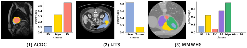
Figure 1: Examples of three benchmarks (i.e., ACDC, LiTS, MMWHS) with long-tail class distributions.

Despite great promise, the main technical challenges remain: (1) How far is CL from becoming a principled framework for medical image segmentation? (2) Is there any better way to implicitly learn some intrinsic properties from the original data (i.e., the inter-instance relationships and intra-instance invariance)? (3) What will happen if models can only access a few labels in training?

To address the above challenges, we outline three principles below: (1) tailness: existing approaches inevitably suffer from class collapse problems – wherein similar pairs from the same latent class are assumed to have the same representation [2, 22, 51]. This assumption, however, rarely holds for real-world clinical data. We observe that the long-tail distribution problem has received increasing attention in the computer vision community [47, 107, 24, 94, 45]. In contrast, there have been a few prior long-tail works for medical image segmentation. For example, as illustrated in Figure 1, most medical image images follow a Zipf long-tail distribution where various anatomical features share very different class frequencies, which can result in worse performance; (2) consistency: considering the scarcity of medical data in practice, augmentations are a widely adopted pre-text task to learn meaningful representations. Intuitively, the anatomical features should be semantically consistent across different transformations and deformations. Thus, it is important to assess whether the model is robust to diverse views of anatomy; (3) diversity: recent work [105, 3, 83] pointed out that going beyond simple augmentations to create more diverse views can learn more discriminative anatomical features. At the same time, this is particularly challenging to both introduce sufficient diversity and preserve the anatomy of the original data, especially in data-scarce clinical scenarios. To deploy into the wild, we need to quantify and address three research gaps from different anatomical views.

In this paper, we present Mine yOur owN Anatomy (MONA), a novel contrastive semi-supervised 2D medical segmentation framework, based on different anatomical views. The workflow of MONA is illustrated in Figure 2. The key innovation in MONA is to seek diverse views (i.e., augmented/mined views) of different samples whose anatomical features are homogeneous within the same class type, while distinctive for different class types. We make the following contributions. First, we consider the problem of tailness. An issue is that label classes within medical images typically exhibit a long-tail distribution. Another one, technically more challenging, is the fact that there is only a few labeled data and large quantities of unlabeled ones during training. Intuitively we would like to sample more pixel-level representations from tail classes. Thus, we go beyond the naïve setting of instance discrimination in CL [19, 40, 37] by decomposing images into diverse and yet consistent anatomical features, each belonging to different classes. In particular, we propose to use pseudo labeling and knowledge distillation to learn better pixel-level representations within multiple semantic classes in a training mini-batch. Considering performing pixel-level CL with medical images is impractical for both memory cost and training time, we then adopt active sampling strategies [57] such as in-batch hard negative pixels, to better discriminate the representations at a larger scale.

We further address the two other challenges: consistency and diversity. The success of the common CL theme is mainly attributed to invariant mapping [38] and instance discrimination [89, 19]. Starting from these two key aspects, we try to further improve the segmentation quality. More specifically, we suggest that consistency to transformation (equivariance) is an effective strategy to establish the invariances (i.e., anatomical features and shape variance) to various image transformations. Furthermore, we investigate two ways to include diversity-promoting views in sample generation. First, we incorporate a memory buffer to alleviate the demand for large batch size, enabling much more efficient training without inhibiting segmentation quality. Second, we leverage stronger augmentations and nearest neighbors to mine views as positive views for more semantic similar contexts.

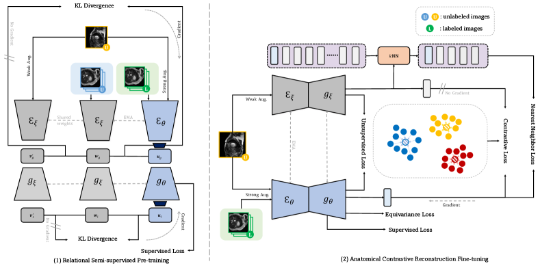
Figure 2: Overview of the MONA framework including two stages: (1) relational semi-supervised pre-training, (2) our proposed anatomical contrastive reconstruction fine-tuning. Note that U and L denote unlabeled and labeled data.

Extensive experiments are conducted on a variety of datasets and the latest CL frameworks (i.e., MoCo [40], SimCLR [19], BYOL [37], and ISD [80]), which consistently demonstrate the effectiveness of our proposed MONA. For example, our MONA establishes the new state-of-the-art performance, compared to all the state-of-the-art semi-supervised approaches with different label ratios (i.e., 1%, 5%, 10%). Moreover, we present a systematic evaluation for analyzing why our approach performs so well and how different factors contribute to the final performance (See Section 4.2). Theoretically, we show the efficacy of our MONA in label efficiency (See Appendix C). Empirically, we also study whether these principles can effectively complement each CL framework (See Appendix D). We hope our findings will provide useful insights on medical image segmentation to other researchers.

To summarise, our contributions are as follows: ❶ we carefully examine the problem of semi-supervised 2D medical image segmentation with extremely limited labels, and identify the three principles to address such challenging tasks; ❷ we construct a set of objectives, which significantly improves the segmentation quality, both long-tail class distribution and anatomical features; ❸ we both empirically and theoretically analyze several critical components of our method and conduct thorough ablation studies to validate their necessity; ❹ with the combination of different components, we establish state-of-the-art under SSL settings, for all the challenging three benchmarks.

2 Related work

Medical Image Segmentation.   Medical image segmentation aims to assign a class label to each pixel in an image, and plays a major role in real-world applications, such as assisting the radiologists for better disease diagnosis and reduced cost. With sufficient annotated training data, significant progress has been achieved with the introduction of Fully convolutional networks (FCN) [58] and UNet [73]. Follow-up works can be categorized into two main directions. One direction is to improve modern segmentation network design. Many CNN-based [77, 41] and Transformer-like [84, 27] model variants [61, 17, 1, 65, 18, 88, 87, 16, 11, 91, 39, 81, 26, 44, 95] have been proposed since then. For example, some works [17, 18, 25] proposed to use dilated/atrous/deformable convolutions with larger receptive fields for more dense anatomical features. Other works [16, 11, 91, 39, 81, 95] include Transformer blocks to capture more long-range information, achieving the impressive performance. A parallel direction is to select proper optimization strategies, by designing loss functions to learn meaningful representations [56, 92, 76]. However, those methods assume access to a large, labeled dataset. This restrictive assumption makes it challenging to deploy in most real-world clinical practices. In contrast, our MONA is more robust as it leverages only a few labeled data and large quantities of unlabeled one in the learning stage.

Semi-Supervised Learning (SSL).   The goal in robust SSL is to improve the medical segmentation performance by taking advantage of large amounts of unlabelled data during training. It can be roughly categorized into three groups: (1) self-training by generating unreliable pseudo-labels for performance gains, such as pseudo-label estimation [49, 4, 28, 21], model uncertainty [98, 35, 46, 60, 99, 63, 10, 12], confidence estimation [8, 33, 48], and noisy student [90]; (2) consistency regularization [9, 23, 30, 29] by integrating consistency corresponding to different transformation, such as pi-model [75], co-training [70, 106], and mean-teacher [79, 71, 50, 103, 54, 72]; (3) other training strategies such as adversarial training [100, 64, 102, 104, 52, 82] and entropy minimization [36]. In contrast to these works, we do not explore more advanced pseudo-labelling strategy to learn spatially structured representations. In this work, we are the first to explore a novel direction for discovering distinctive and semantically consistent anatomical features without image-level or region-level labels. Further, we expect that our findings can be relevant for other medical image segmentation frameworks.

Contrastive Learning.   CL has recently emerged as a promising paradigm for medical image segmentation via exploiting abundant unlabeled data, leading to state-of-the-art results [14, 96, 15, 43, 50, 71, 97]. The high-level idea of CL is to pull closer the different augmented views of the same instance but pushes apart all the other instances away. Intuitively, differently augmented views of the same image are considered positives, while all the other images serve as negatives. The major difference between different CL-based frameworks lies in the augmentation strategies to obtain positives and negatives. A few very recent studies [47, 45] confirm the superiority of CL of addressing imbalance issues in image classification. Moreover, existing CL frameworks [14, 96] mainly focus on the instance level discrimination (i.e., different augmented views of the same instance should have similar anatomical features or clustered around the class weights). However, we argue that not all negative samples equally matter, and the above issues have not been explored from the perspective of medical image segmentation, considering the class distributions in the medical image are perspectives diverse and always exhibit long tails [34, 93, 74]. Inspired by the aforementioned, we address these two issues in medical image segmentation - two appealing perspectives that still remain under-explored.

3 Mine yOur owN Anatomy (MONA)

3.1 Framework

Overview.   We introduce our contrastive learning framework (See Figure 2), which includes (1) relational semi-supervised pre-training, and (2) anatomical contrastive reconstruction fine-tuning. The key idea is to seek diverse yet semantically consistent views whose anatomical features are homogeneous within the same class type, while distinctive for different class types. In this paper, our pre-training stage is built upon ISD [80] - a competitive framework for image classification. The main differences between ISD and MONA are: MONA is more tailored to medical image segmentation, i.e., considering the dense nature of this problem both in global and local manner, and can generalize well to those long-tail scenarios. Also, our principles are expected to apply to other CL framework ((i.e., MoCo [40], SimCLR [19], BYOL [37]). More detailed empirical and theoretical analysis can be found in Appendix D and Appendix C.

Pre-training preliminary.   Let $(X,Y)$ be our dataset, including training images ${\bf x}\in X$ and their corresponding $\mathcal{C}$-class segmentation labels ${\bf y}\in Y$, where $X$ is composed of $N$ labeled and $M$ unlabeled slices. Note that, for brevity, ${\bf y}$ can be either sampled from $Y$ or pseudo-labels. The student and teacher networks $\mathcal{F}$, parameterized by weights $\theta$ and $\xi$, each consist of a encoder $\mathcal{E}$ and a decoder $\mathcal{D}$ (i.e., UNet [73]). Concretely, given a sample ${\bf s}$ from our unlabeled dataset, we have two ways to generate views: (1) we formulate augmented views (i.e., ${\bf x},{\bf x}^{\prime}$) through two different augmentation chains; and (2) we create $d$ mined views (i.e., ${\bf x}_{r,i}$) by randomly selecting from the unlabeled dataset followed by additional augmentation. We then fed the augmented views to both $\mathcal{F}_{\theta}$ and $\mathcal{F}_{\xi}$, and the mined views to $\mathcal{F}_{\xi}$. Similar to [14], we adopt the global and local instance discrimination strategies in the latent and output feature spaces. Specifically, the encoders generate global features ${\bf z}_{g}={\mathcal{E}}_{\theta}({\bf x})$, ${\bf z}^{\prime}_{g}={\mathcal{E}}_{\xi}({\bf x}^{\prime})$, and ${\bf z}_{r,g}={\mathcal{E}}_{\xi}({\bf x}_{r})$, which are then fed into the nonlinear projection heads to obtain ${\bf v}_{g}=h_{\theta}({\bf z}_{g})$, ${\bf v}^{\prime}_{g}=h_{\xi}({\bf z}^{\prime}_{g})$, and ${\bf w}_{g}=h_{\xi}({\bf z}_{r,g})$. The augmented embeddings from the student network are further projected into secondary space, i.e., ${{\bf u}_{g}}=h^{\prime}_{\theta}({\bf v}_{g})$. We calculate similarities across mined views and augmented views from the student and teacher in both global and local manners. Then a softmax function is applied to process the calculated similarities, which models the relationship distributions:

$${\bf s}_{\theta} =\text{log}\frac{\text{exp}\big{(}\text{sim}\big{(}{\bf u},{\bf w}\big{)}/\tau_{\theta}\big{)}}{\sum_{j=1}^{k}\text{exp}\big{(}\text{sim}\big{(}{\bf u},{\bf w}_{j}\big{)}/\tau_{\theta}\big{)}},\quad$$ (3.1)

$${\bf s}_{\xi} =\text{log}\frac{\text{exp}\big{(}\text{sim}\big{(}{\bf v}^{\prime},{\bf w}\big{)}/\tau_{\xi}\big{)}}{\sum_{j=1}^{k}\text{exp}\big{(}\text{sim}\big{(}{\bf v}^{\prime},{\bf w}_{j}\big{)}/\tau_{\xi}\big{)}},$$

where $\tau_{\theta}$ and $\tau_{\xi}$ are different temperature parameters, and $\text{sim}(\cdot,\cdot)$ denotes cosine similarity. The unsupervised instance discrimination loss (i.e., Kullback-Leibler divergence $\mathcal{KL}$) can be defined as:

$$\mathcal{L}_{\text{inst}}=\mathcal{KL}({\bf s}_{\theta}||{\bf s}_{\xi}).$$ (3.2)

The parameters $\xi$ of $\mathcal{F}_{\xi}$ is updated as: $\xi=t\xi+(1-t)\theta$ with $t=0.99$ as a momentum hyperparameter. In our pre-training stage, the total loss is the sum of global and local instance discrimination loss $\mathcal{L}_{\text{inst}}$ (on pseudo-labels), and supervised segmentation loss $\mathcal{L}_{\text{sup}}$ (i.e., equal combination of dice loss and cross-entropy loss on ground-truth labels): $\mathcal{L^{\text{global}}_{\text{inst}}}+\mathcal{L^{\text{local}}_{\text{inst}}}+\mathcal{L}_{\text{sup}}$.

Principles.   As shown in Figure 2, the principles behind MONA (i.e., the second anatomical contrastive reconstruction stage) aim to ensure tailness, consistency, and diversity. Concretely, tailness is for actively sampling more tail class hard pixels; consistency ensures the feature invariances; and diversity further encourages to discover more anatomical features in different images. More theoretical analysis is in Appendix C.

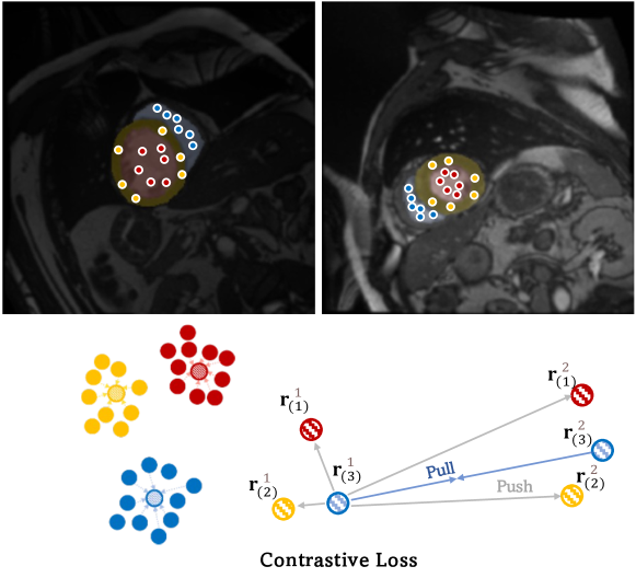
Figure 3: Illustration of the contrastive loss.

3.2 Anatomical Contrastive Reconstruction

Tailness.   Motivated by the observations (Figure 1), our primary cue is that medical images naturally exhibit an imbalanced or long-tailed class distribution, wherein many class labels are associated with only a few pixels. To generalize well on such imbalanced setting, we propose to use anatomical contrastive formulation (ACF) (See Figure 3).

Here we additionally attach the representation heads to fuse the multi-scale features with the feature pyramid network (FPN) [55] structure and generate the $m$-dimensional representations with consecutive convolutional layers. The high-level idea is that the features should be very similar among the same class type, while very dissimilar across different class types. Particularly for long-tail medical data, a naïve application of this idea would require substantially computational resources proportional to the square of the number of pixels within the dataset, and naturally overemphasize the anatomy-rich head classes and leaves the tail classes under-learned in learning invariances, both of which suffer performance drops.

To this end, we address this issue by actively sampling a set of pixel-level anchor representations ${\bf r}_{q}\in\mathcal{R}_{q}^{c}$ (queries), pulling them closer to the class-averaged mean of representations ${\bf r}_{k}^{c,+}$ within this class $c$ (positive keys), and pushing away from representations ${\bf r}_{k}^{-}\in\mathcal{R}_{k}^{c}$ from other classes (negative keys). Formally, the contrastive loss is defined as:

$$\mathcal{L}_{\text{contrast}} =\sum_{c\in\mathcal{C}}\sum_{{\bf r}_{q}\sim\mathcal{R}^{c}_{q}}$$ (3.3)

$$-\log\frac{\exp({\bf r}_{q}\cdot{\bf r}_{k}^{c,+}/\tau)}{\exp({\bf r}_{q}\cdot{\bf r}_{k}^{c,+}/\tau)+\sum_{{\bf r}_{k}^{-}\sim\mathcal{R}^{c}_{k}}\exp({\bf r}_{q}\cdot{\bf r}_{k}^{-}/\tau)},$$

where $\mathcal{C}$ denotes a set of all available classes for each mini-batch, and $\tau$ is a temperature hyperparameter. Suppose $\mathcal{A}$ is a collection including all pixel coordinates within ${\bf x}$, these representations are:

$$\mathcal{R}_{q}^{c} =\bigcup_{[m,n]\in\mathcal{A}}\!\!\mathbbm{1}({\bf y}_{[m,n]}\!=\!c)\,{\bf r}_{[m,n]},\,$$ (3.4)

$$\mathcal{R}_{k}^{c} =\bigcup_{[m,n]\in\mathcal{A}}\!\!\mathbbm{1}({\bf y}_{[m,n]}\!\neq\!c)\,{\bf r}_{[m,n]},\,$$

$${\bf r}_{k}^{c,+} =\frac{1}{|\mathcal{R}_{q}^{c}|}\sum_{{\bf r}_{q}\in\mathcal{R}_{q}^{c}}{\bf r}_{q}\,.$$

We then note that CL might benefit more, where the instance discrimination task is achieved by incorporating more positive and negative pairs. However, naively unrolling CL to this setting is impractical since it requires extra memory overheads that grow proportionally with the amount of instance discrimination tasks. To this end, we adopt a random set (i.e., the mini-batch) of other images. Intuitively, we would like to maximize the anatomical similarity between all the representations from the query class, and analogously minimize all other class representations. We then create a graph $\mathcal{G}$ to compute the pair-wise class relationship: $\mathcal{G}[p,q]=\left({\bf r}_{k}^{p,+}\cdot{\bf r}_{k}^{q,+}\right),\forall p,q\in\mathcal{C},\text{ and }p\neq q,$ where $\mathcal{G}\in\mathbb{R}^{|\mathcal{C}|\times|\mathcal{C}|}$. Here finding the accurate decision boundary can be formulated mathematically by normalizing the pair-wise relationships among all negative class representations via the softmax operator. To address the challenge in imbalanced medical image data, we define the pseudo-label (i.e., easy and hard queries) based on a defined threshold as follows:

$$\begin{split}\mathcal{R}_{q}^{c,\,\text{easy}}&=\bigcup_{{\bf r}_{q}\in\mathcal{R}^{c}_{q}}\mathbbm{1}(\widehat{{\bf y}}_{q}>\delta_{\theta}){\bf r}_{q},\quad\\ \mathcal{R}_{q}^{c,\,\text{hard}}&=\bigcup_{{\bf r}_{q}\in\mathcal{R}^{c}_{q}}\mathbbm{1}(\widehat{{\bf y}}_{q}\leq\delta_{\theta}){\bf r}_{q},\end{split}$$ (3.5)

where $\widehat{{\bf y}}_{q}$ is the $c^{\text{th}}$-class pseudo-label corresponding to ${\bf r}_{q}$, and $\delta_{\theta}$ is the user-defined threshold. For further improvement in long-tail scenarios, we construct a class-aware memory bank [40] to store a fixed number of negative samples per class $c$.

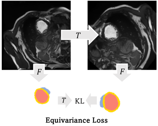
Figure 4: Illustration of the equivariance loss.

Table 1: Comparison of segmentation performance (DSC[%]/ASD[mm]) on ACDC and LiTS under three labeled ratio settings (1%, 5%, 10%). The best results are indicated in bold.

ACDC LiTS 1% Labeled 5% Labeled 10% Labeled 1% Labeled 5% Labeled 10% Labeled Method DSC $\uparrow$ ASD $\downarrow$ DSC $\uparrow$ ASD $\downarrow$ DSC $\uparrow$ ASD $\downarrow$ DSC $\uparrow$ ASD $\downarrow$ DSC $\uparrow$ ASD $\downarrow$ DSC $\uparrow$ ASD $\downarrow$ UNet-F [73] 91.5 0.996 91.5 0.996 91.5 0.996 68.5 17.8 68.5 17.8 68.5 17.8 UNet-L 14.5 19.3 51.7 13.1 79.5 2.73 57.0 34.6 60.4 30.4 61.6 28.3 EM [86] 21.1 21.4 59.8 5.64 75.7 2.73 56.6 38.4 61.2 33.3 62.9 38.5 CCT [67] 30.9 28.2 59.1 10.1 75.9 3.60 52.4 52.3 60.6 48.7 63.8 31.2 DAN [100] 34.7 25.7 56.4 15.1 76.5 3.01 57.2 27.1 62.3 25.8 63.2 30.7 URPC [59] 32.2 26.9 58.9 8.14 73.2 2.68 55.5 34.6 62.4 37.8 63.0 43.1 DCT [70] 36.0 24.2 58.5 10.8 78.1 2.64 57.6 38.5 60.8 34.4 61.9 31.7 ICT [85] 35.8 21.3 59.0 4.59 75.1 0.898 58.3 32.2 60.1 39.1 62.5 32.4 MT [79] 36.8 19.6 58.3 11.2 80.1 2.33 56.7 34.3 61.9 40.0 63.3 26.2 UAMT [98] 35.2 24.3 61.0 7.03 77.6 3.15 57.8 41.9 61.0 47.0 62.3 26.0 CPS [21] 37.1 30.0 61.0 2.92 78.8 3.41 57.7 39.6 62.1 36.0 64.0 23.6 GCL [14] 59.7 14.3 70.6 2.24 87.0 0.751 59.3 29.5 63.3 20.1 65.0 37.2 SCS [43] 59.4 12.7 73.6 5.37 84.2 2.01 57.8 39.6 61.5 28.8 64.6 33.9 PLC [15] 58.8 15.1 70.6 2.67 87.3 1.34 56.6 41.6 62.7 26.1 68.2 16.9 $\bullet$ MONA (ours) 82.6 2.03 88.8 0.622 90.7 0.864 64.1 20.9 67.3 16.4 69.3 18.0

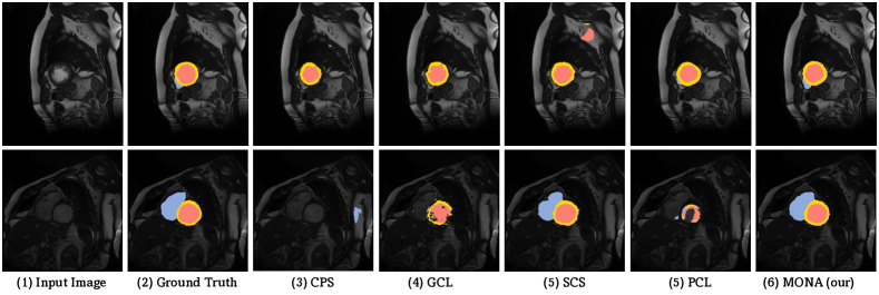
Figure 5: Visualization of segmentation results on ACDC with 5% label ratio. As is shown, MONA consistently yields more accurate predictions and better boundary adherence compared to all other SSL methods. Different anatomical classes are shown in different colors (RV: ; Myo: ; LV: ).

Consistency.   The proposed ACF is designed to address imbalanced issues, but anatomical consistency remains to be weak in the long-tail medical image setting since medical segmentation should be robust to different tissue types which show different anatomical variations. As shown in Figure 4, we hence construct a random image transformation $\mathcal{T}$ and define the equivariance loss on both labeled and unlabeled data by measuring the feature consistency distance between each original segmentation map and the segmentation map generated from the transformed image:

$$\mathcal{L}_{\text{eqv}}({\bf x},\mathcal{T}({\bf x})) =\sum_{{\bf x}\in X}\mathcal{KL}\left(\mathcal{T}(\mathcal{F}_{\theta}({\bf x})),\mathcal{F}_{\theta}(\mathcal{T}({\bf x}))\right)$$ (3.6)

$$+\mathcal{KL}\left(\mathcal{F}_{\theta}(\mathcal{T}({\bf x})),\mathcal{T}(\mathcal{F}_{\theta}({\bf x}))\right)\,.$$

Here we define $\mathcal{T}$ on both the input image ${\bf x}$ and $\mathcal{F}_{\theta}({\bf x})$, via the random transformations (i.e., affine, intensity, and photo-metric augmentations), since the model should learn to be robust and invariant to these transformations.

Diversity.   Oversampling too many images from the random set would create extra memory overhead, and more importantly, our finding also uncovers that a large number of random images might not necessarily help impose additional invariances between neighboring samples since redundant images might introduce additional noise during training (see the Appendix E). In contrast to sampling from latent space, we perform in the output space. Therefore, we formulate our insight as an auxiliary loss that regularizes the representations - keeping the anatomical contrastive reconstruction task as the main force. In practice, we first search for $K$-nearest neighbors from the first-in-first-out (FIFO) memory bank [40], and then use the nearest neighbor loss $\mathcal{L}_{\text{nn}}$ in a way that maximizing cosine similarity, to exploit the inter-instance relationship.

Setup.   The total loss $\mathcal{L}_{\text{total}}$ is the sum of contrastive loss $\mathcal{L}_{\text{contrast}}$ (on both ground-truth labels and pseudo-labels), equivariance loss $\mathcal{L}_{\text{eqv}}$ (on both ground-truth labels and pseudo-labels), nearest neighbors loss $\mathcal{L}_{\text{nn}}$ (on both ground-truth labels and pseudo-labels), unsupervised cross-entropy loss $\mathcal{L}_{\text{unsup}}$ (on pseudo-labels) and supervised segmentation loss $\mathcal{L}_{\text{sup}}$ (on ground-truth labels): $\mathcal{L}_{\text{sup}}+\lambda_{1}\mathcal{L_{\text{contrast}}}+\lambda_{2}\mathcal{L}_{\text{eqv}}+\lambda_{3}\mathcal{L}_{\text{unsup}}+\lambda_{4}\mathcal{L}_{\text{nn}}$. We theoretically analyze the effectiveness of our MONA in the very limited label setting (See Appendix C). We also empirically conduct ablations on different hyperparameters (See Appendix E).

4 Experiments

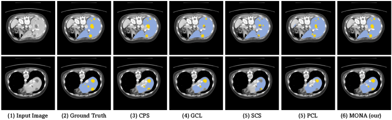
Figure 6: Visualization of segmentation results on LiTS with 5% labeled ratio. As is shown, MONA consistently produces sharp and accurate object boundaries compared to all other SSL methods. Different anatomical classes are shown in different colors (Liver: ; Tumor: ).

In this section, we evaluate our proposed MONA on three popular medical image segmentation datasets under varying labeled ratio settings: the ACDC dataset [6], the LiTS dataset [7], and the MMWHS dataset [108] (See Appendix B). Moreover, to further validate our approach’s unsupervised imbalance handling ability, we consider a more realistic and more challenging scenario, wherein the models would only have access to the extremely limited labeled data (i.e., 1% labeled ratio) and large quantities of unlabeled one in training. For all experiments, we follow the same training and testing protocol. Note that 1%, 5%, and 10% label ratios denote the ratio of patients. For ACDC, we adopt the fixed data split. For LiTS and MMWHS, we adopt the random data split with respect to patient. All three splitting details are in the supplementary material. See Appendix A for more implementation details.

4.1 Main Results

We show the effectiveness of our method under three different label ratios (i.e., 1%, 5%, 10%). We also compare MONA with various state-of-the-art SSL and fully-supervised methods on three datasets: ACDC [6], LiTS [7], MMWHS [108]. We choose 2D UNet [73] as backbone, and compare against SSL methods including UNet trained with full/limited supervisions (UNet-F/UNet-L), EM [86], CCT [67], DAN [100], URPC [59], DCT [70], ICT [85], MT [79], UAMT [98], CPS [21], SCS [43], GCL [14], and PLC [15]. We report quantitative comparisons on ACDC and LiTS in Table 1, and average all our results over three runs. (More results on MMWHS in Appendix B).

ACDC.   We benchmark performances on ACDC with respect to different labeled ratios (i.e., 1%, 5%, 10%). The following observations can be drawn: First, our proposed MONA significantly outperforms all other SSL methods under three different label ratios. Especially, with only extremely limited labeled data available (e.g., 1%), our method obtains massive gains of 82.6% and 2.03 in Dice and ASD (i.e., dramatically improving the performance from 59.4% to 82.6%). Second, as shown in Figure 5, we can see the clear advantage of MONA, where the anatomical boundaries of different tissues are clearly more pronounced such as RV and Myo regions. As seen, our method is capable of producing consistently sharp and accurate object boundaries across various challenge scenarios.

LiTS.   We then evaluate MONA on LiTS, using 1%, 5%, 10% labeled ratios. The results are summarized in Table 1 and Figure 6. The conclusions we can draw are highly consistent with the above ACDC case: First, at the different label ratios (i.e., 1%, 5%, 10%), MONA consistently outperforms all the other SSL methods, which again demonstrates the effectiveness of learning representations for the inter-class correlations and intra-class invariances under imbalanced class-distribution scenarios. In particular, our MONA, trained on a 1% labeled ratio (i.e., extremely limited labels), dramatically improves the previous best averaged Dice score from 59.3% to 64.1% by a large margin, and even performs on par with previous SSL methods using 10% labeled ratio. Second, our method consistently outperforms all the evaluated SSL methods under different label ratios (i.e., 1%, 5%, 10%). Third, as shown in Figure 6, we observe that MONA is able to produce more accurate results compared to the previous best schemes.

4.2 Ablation Study

In this subsection, we conduct comprehensive analyses to understand the inner workings of MONA on ACDC under 5% labeled ratio. Note that for reproducibility, we report the average performance of three independent runs with different random seeds. More results and details about our case study are referred to the Appendix D and E.

Effects of Different Components.   Our key observation is that it is crucial to build meaningful anatomical representations for the inter-class correlations and intra-class invariances under imbalanced class-distribution scenarios can further improve performance. Upon our choice of architecture, we first consider our proposed CL pre-trained method (i.e., GLCon). To validate this, we experiment with the key components in MONA on ACDC, including: (1) tailness, (2) consistency, and (3) diversity. The results are in Table 2. As is shown, each key component makes a clear difference and leveraging all of them contributes to the remarkable performance improvements. This suggests the importance of learning meaningful representations for the inter-class correlations and intra-class invariances within the entire dataset. The intuitions behind each concept are as follows: (1) Only tailness: many anatomy-rich head classes would be sampled; (2) Only consistency: it would lead to object collapsing due to the different anatomical variations; (3) Only diversity: oversampling too many negative samples often comes at the cost of performance degradation. By combining tailness, consistency, and diversity, our method confers a significant advantage at representation learning in imbalanced feature similarity, semantic consistency and anatomical diversity, which further highlights the superiority of our proposed MONA (More results in Appendix D).

Table 2: Ablation on model component: (1) tailness; (2) consistency; (3) diversity, compared to the Vanilla and our MONA.

Method	Metrics
	Dice[%] $\uparrow$	ASD[mm] $\downarrow$
Vanilla	74.2	3.89
w/ tailness	83.1	0.602
w/ consistency	84.2	1.86
w/ diversity	78.2	3.07
w/ tailness + consistency	88.1	0.864
w/ consistency + diversity	80.2	2.11
w/ tailness + diversity	85.0	0.913
$\bullet$ MONA (ours)	88.8	0.622

Effects of Different Augmentations.   In addition to further improving the quality and stability in anatomical representation learning, we claim that MONA also gains robustness using augmentation strategies. For augmentation strategies, previous works [80, 105, 78] show that composing the weak augmentation strategy for the “pivot-to-target” model (i.e., trained with limited labeled data and a large number of unlabeled data) is helpful for anatomical representation learning since the standard contrastive strategy is too aggressive, intuitively leading to a “hard” task (i.e., introducing too many disturbances and yielding model collapses). Here we examine whether and how applying different data augmentations helps MONA. In this work, we implement the weak augmentation to the teacher’s input as random rotation, random cropping, horizontal flipping, and strong augmentation to the student’s input as random rotation, random cropping, horizontal flipping, random contrast, CutMix [31], brightness changes [69], morphological changes (diffeomorphic deformations). We summarize the results in Table 3, and list the following observations: (1) weak augmentations benefits more: composing the weak augmentation for the teacher model and strong augmentation for the student model significantly boosts the performance across two benchmark datasets. (2) same augmentation pairs do not make more gains: interestingly, applying same type of augmentation pairs does not lead to the best performance compared to different types of augmentation pairs. We postulate that composing different augmentations can be considered as a harder albeit more useful strategy for anatomical representation learning, making feature more generalizable.

Table 3: Ablation on augmentation strategies for MONA on the ACDC and LiTS dataset under 5% labeled ratio.

Dataset		Student Teacher		Metrics
		Aug. Aug.		Dice[%] $\uparrow$	ASD[mm] $\downarrow$
ACDC		Weak	Weak	86.0	1.02
		Strong	Weak	88.8	0.622
		Weak	Strong	86.4	2.83
		Strong	Strong	88.8	2.07
LiTS		Weak	Weak	62.3	26.5
		Weak	Strong	67.3	16.4
		Strong	Weak	64.3	34.7
		Strong	Strong	66.5	21.1

Extra Study.   More investigations about (1) generalization across CL frameworks; (2) theoretical analysis; (3) ablation on different training settings are in Appendix D, C, and E.

5 Conclusion

In this paper, we have presented MONA, a semi-supervised contrastive learning method for 2D medical image segmentation. We start from the observations that medical image data always exhibit a long-tail class distribution, and the same anatomical objects (i.e., liver regions for two people) are more similar to each other than different objects (e.g.liver and tumor regions). We further expand upon this idea by introducing anatomical contrastive formulation, as well as equivariance and invariances constraints. Both empirical and theoretical studies show that we can formulate a generic set of perspectives that allows us to learn meaningful representations across different anatomical features, which can dramatically improve the segmentation quality and alleviate the training memory bottleneck. Extensive experiments on three datasets demonstrate the superiority of our proposed framework in the long-tailed medical data regimes with extremely limited labels. We believe our results contribute to a better understanding of medical image segmentation and point to new avenues for long-tailed medical image data in realistic clinical applications.

Appendix

Appendix A More Training Details

A.1 Datasets

The ACDC dataset was hosted in MICCAI 2017 ACDC challenge [6], which includes 200 3D cardiac cine MRI scans with expert annotations for three classes (i.e., left ventricle (LV), myocardium (Myo), and right ventricle (RV)). We use 120, 40 and 40 scans for training, validation, and testing. Note that 1%, 5%, and 10% label ratios denote the ratio of patients. For pre-processing, we adopt the similar setting in [14] by normalizing the intensity of each 3D scan (i.e., using min-max normalization) into $[0,1]$, and re-sampling all 2D scans and the corresponding segmentation maps into a fixed spatial resolution of $256\times 256$ pixels.

The LiTS dataset was hosted in MICCAI 2017 Liver Tumor Segmentation Challenge [7], which includes 131 contrast-enhanced 3D abdominal CT volumes with expert annotations for two classes (i.e., liver and tumor). Note that 1%, 5%, and 10% label ratios denote the ratio of patients. We use 100 and 31 scans for training, and testing with random order. The splitting details are in the supplementary material. For pre-processing, we adopt the similar setting in [53] by truncating the intensity of each 3D scan into $[-200,250]$ HU for removing irrelevant and redundant details, normalizing each 3D scan into $[0,1]$, and re-sampling all 2D scans and the corresponding segmentation maps into a fixed spatial resolution of $256\times 256$ pixels.

The MMWHS dataset was hosted in MICCAI 2017 challenge [108], which includes 20 3D cardiac MRI scans with expert annotations for seven classes: left ventricle (LV), left atrium (LA), right ventricle (RV), right atrium (RA), myocardium (Myo), ascending aorta (AAo), and pulmonary artery (PA). Note that 1%, 5%, and 10% label ratios denote the ratio of patients. We use 15 and 5 scans for training and testing with random order. The splitting details are in the supplementary material. For pre-processing, we normalize the intensity of each 3D scan (i.e., using min-max normalization) into $[0,1]$, and re-sampling all 2D scans and the corresponding segmentation maps into a fixed spatial resolution of $256\times 256$ pixels.

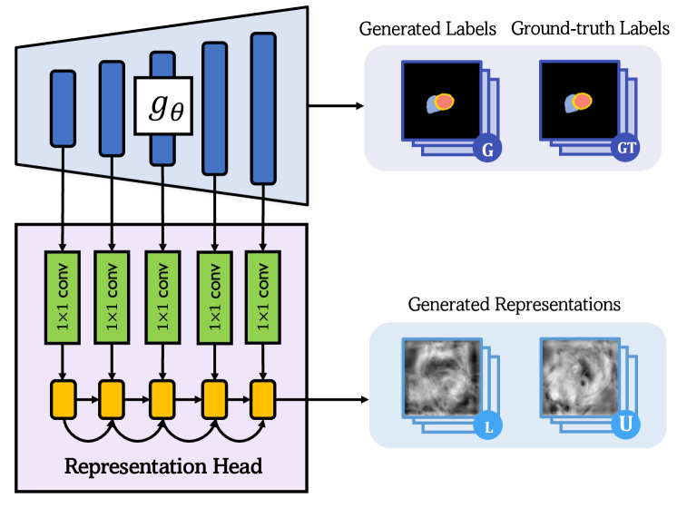
Figure 7: Representation head architecture.

Table 4: Comparison of segmentation performance (DSC[%]/ASD[mm]) on MMWHS under three labeled ratio settings (1%, 5%, 10%). On all three labeled settings, MONA significantly outperforms all the state-of-the-art methods by a significant margin. The best results are in bold.

1% Labeled 5% Labeled 10% Labeled Method DSC $\uparrow$ ASD $\downarrow$ DSC $\uparrow$ ASD $\downarrow$ DSC $\uparrow$ ASD $\downarrow$ UNet-F [73] 85.8 8.01 85.8 8.01 85.8 8.01 UNet-L 58.3 33.9 77.8 24.4 82.7 13.5 EM [86] 54.5 41.1 80.6 17.3 82.1 15.1 CCT [67] 62.8 27.5 79.0 21.9 79.4 16.3 DAN [100] 52.8 48.4 79.4 22.7 80.2 15.0 URPC [59] 65.7 29.7 73.7 20.5 81.9 12.3 DCT [70] 62.7 27.5 80.8 23.0 82.8 12.4 ICT [85] 59.9 32.8 76.5 15.4 82.2 12.0 MT [79] 58.8 35.6 76.5 15.5 79.4 19.8 UAMT [98] 61.1 37.6 76.3 20.9 83.7 14.2 CPS [21] 58.8 33.6 78.3 22.5 82.0 13.1 GCL [14] 71.6 20.3 83.5 7.41 86.7 8.76 SCS [43] 71.4 19.3 81.1 11.5 82.6 9.68 PLC [15] 71.5 19.8 83.4 10.7 86.0 9.65 $\bullet$ MONA (ours) 83.9 9.06 86.3 8.22 87.6 6.83

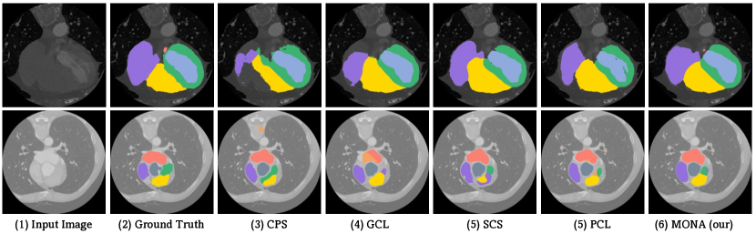
Figure 8: Visualization of segmentation results on MMWHS with 5% labeled ratio. As is shown, MONA consistently generates more accurate predictions compared to all other SSL methods with a significant performance margin. Different anatomical classes are shown in different colors (LV: ; LA: ; RV: ; RA: ; Myo: ; PA: ).

A.2 Implementation Details.

We implement all the evaluated models using PyTorch library [68]. All the models are trained using Stochastic Gradient Descent (SGD) (i.e., initial learning rate = $0.01$, momentum = $0.9$, weight decay = $0.0001$) with batch size of $6$, and the initial learning rate is divided by $10$ every $2500$ iterations. All of our experiments are conducted on NVIDIA GeForce RTX 3090 GPUs. We first train our model with 100 epochs during the pre-training, and then retrain the model for 200 epochs during the fine-tuning. We set the temperature $\tau_{\xi}$, $\tau_{\theta}$, $\tau$ as 0.01, 0.1, 0.5. The size of the memory bank is 36. During the pre-training, we follow the settings of ISD, including global projection head setting, and predictors with the $512$-dimensional output embedding, and adopt the setting of local projection head in [43]. More specifically, given the predicted logits $\widehat{{\bf y}}\in\mathbb{R}^{\mathcal{C}\times\mathcal{H}\times\mathcal{W}}$, we create 36 different views (i.e., random crops at the same location) of $\widehat{{\bf y}}$ and $\widehat{{\bf y}}^{\prime}$ with the fixed size $64\times 64$, and then project all pixels into $512$-dimensional output embedding space, and the output feature dimension of $h^{\prime}_{\theta}$ is also $512$. An illustration of our representation head is presented in Figure 7. We then actively sample 256 query embeddings and 512 key embeddings for each mini-batch, and the confidence threshold $\delta_{\theta}$ is set to $0.97$. When fine-tuning we use an equally sized pool of candidates $K=5$, as well as $\lambda_{1}=0.01$, $\lambda_{2}=1.0$, $\lambda_{3}=1.0$, and $\lambda_{4}=1.0$. For different augmentation strategies, we implement the weak augmentation to the teacher’s input as random rotation, random cropping, horizontal flipping, and strong augmentation to the student’s input as random rotation, random cropping, horizontal flipping, random contrast, CutMix [31], brightness changes [69], morphological changes (diffeomorphic deformations). We adopt two popular evaluation metrics: Dice coefficient (DSC) and Average Symmetric Surface Distance (ASD) for 3D segmentation results. Of note, the projection heads, the predictor, and the representation head are only used in training, and will be discarded during inference.

Table 5: Ablation study of different contrastive learning frameworks on ACDC under three labeled ratio settings (1%, 5%, 10%). We compare two settings: with or without fine-tuning on the segmentation performance (DSC[%]/ASD[mm]). We denote ‘without fine-tuning” to only pretaining. On all three labeled settings, our methods (i.e., GLCon and MONA) significantly outperform all the state-of-the-art methods by a significant margin. All the experiments are run with three different random seeds. The best results are in bold.

1% Labeled 5% Labeled 10% Labeled Framework Method DSC $\uparrow$ ASD $\downarrow$ DSC $\uparrow$ ASD $\downarrow$ DSC $\uparrow$ ASD $\downarrow$ only pretaining MoCov2 [20] 38.6 22.4 56.2 17.9 81.0 5.36 $k$NN-MoCo [83] 39.5 22.0 58.3 15.7 83.1 7.18 SimCLR [19] 34.8 24.3 51.7 19.9 80.3 4.16 BYOL [37] 35.9 7.25 65.9 9.15 85.6 2.51 ISD [80] 45.8 17.2 71.0 4.29 85.3 2.97 $\mathbf{\circ}$ GLCon (ours) 49.3 7.11 74.2 3.89 86.5 1.92 w/ fine-tuning MoCov2 [20] 77.7 4.78 85.4 1.52 86.7 1.74 $k$NN-MoCo [83] 78.0 4.28 85.9 1.51 86.9 1.61 SimCLR [19] 75.7 4.33 83.2 2.06 86.1 2.25 BYOL [37] 77.1 4.84 85.3 2.06 88.1 0.994 ISD [80] 80.1 3.00 83.8 1.95 88.6 1.20 $\bullet$ MONA (ours) 82.6 2.03 88.8 0.622 90.7 0.864

Appendix B More Experiments Results - MMWHS

Lastly, we validate MONA on MMWHS, under 1%, 5%, 10% labeled ratios. The results are provided in Table 4 and Figure 8. Again, we found that MONA consistently outperforms all other SSL methods with a significant performance margin, and achieves the highest accuracy among all the SSL approaches under three labeled ratios. As is shown, MONA trained at the 1% labeled ratio significantly outperforms all other SSL methods trained at the 1% labeled ratio, even over the 5% labeled ratio. Concretely, MONA trained at only 1% labeled ratio outperforms the second-best method (i.e., GLCon) both at the 1% and 5% labeled, yielding 12.3% and 0.4% gains in Dice. We also observe the similar patterns that, MONA performs better than all the other SSL methods at 10% labeled, which again demonstrates the superiority of MONA in extremely limited labeled data regimes.

Appendix C Theoretical Analysis

In this section, we provide a theoretical justification for our MONA. We will focus on exploring how the student-teacher architecture in MONA functions in a way that helps the model generalizes well in the limited-label setting.

To begin with, we introduce some notations and definitions to facilitate our analysis in this section. We denote an image by $\mathbf{x}$ and its label (segmentation map) by $\mathbf{y}$. A segmentation model is a function $f$ such that $f(\mathbf{x})$ is an output segmentation of the image $\mathbf{x}$. Let a (supervised) loss function be denoted by $\ell(\cdot)$, such that the loss of a model $f(\cdot)$ for a sample $(\mathbf{x},\mathbf{y})$ is given as $\ell(f(\mathbf{x}),\mathbf{y})$. Here for generality, we do not specify the exact form of $\ell$, and $\ell$ can be taken as cross-entropy loss, DICE loss, etc.

Since MONA is a semi-supervised framework, we start by considering the supervised part. Specifically, we adopt the typical setting of empirical risk minimization (ERM). Assume there are $n$ data labeled samples $\mathcal{S}_{n}=\{\mathbf{x}_{i},\mathbf{y}_{i}\}_{i=1}^{n}$ from some population distribution $\mathcal{D}$. Let $\mathcal{F}$ denote a function class that contains all the candidate models (e.g., parameterized family of neural networks). The empirical risk of a model $f$ (i.e.supervised training loss) is defined as:

$$R_{\ell,f}(\mathcal{S}_{n})=\frac{1}{n}\sum_{i=1}^{n}\ell(f(\mathbf{x}_{i}),\mathbf{y}_{i}).$$

Supervised learning learns a model by ERM:

$$\widehat{f}=\arg\min_{f\in\mathcal{F}}R_{\ell,f}(\mathcal{S}_{n}).$$

Rademacher complexity

To understand how ERM in the supervised part of MONA is related to its generalization ability, we invoke the tool of Rademacher complexity.

For any function class $\mathcal{G}$, its Rademacher complexity is defined as follows:

Definition C.1 (Rademacher complexity).

Assume there is a labeled sample set $\mathcal{S}_{n}=\{\mathbf{x}_{i},\mathbf{y}_{i}\}_{i=1}^{n}$, such that $(\mathbf{x}_{i},\mathbf{y}_{i})$ are $i.i.d.$ samples from some population distribution $\mathcal{D}$. Let $\sigma=\{\sigma_{i}\}_{i=1}^{n}$ be $i.i.d.$ Bernoulli random variables. The empirical Rademacher complexity $\mathfrak{R}_{\mathcal{S}_{n}}(\mathcal{G})$ is defined as:

$$\mathfrak{R}_{\mathcal{S}_{n}}(\mathcal{G})=\frac{1}{n}\mathbb{E}_{\sigma}\left[\sup_{g\in\mathcal{G}}\sum_{i=1}^{n}\sigma_{i}g(\mathbf{x}_{i},\mathbf{y}_{i})\right].$$

The Rademacher complexity $\mathfrak{R}_{n}(\mathcal{G})$ is defined as:

$$\mathfrak{R}_{n}(\mathcal{G})=\mathbb{E}_{\mathcal{S}_{n}\sim\mathcal{D}^{n}}[\mathfrak{R}_{\mathcal{S}_{n}}(\mathcal{G})].$$

The model function class $\mathcal{F}$ and the loss function $\ell$ together induce a function class $\mathcal{G}_{\ell,\mathcal{F}}$ defined as:

$$\mathcal{G}_{\ell,\mathcal{F}}=\left\{g:(\mathbf{x},\mathbf{y})\to\ell(f(\mathbf{x}),\mathbf{y})\ \middle|\ f\in\mathcal{F}\right\}.$$

The power of Rademacher complexity is that it can relate the generalization ability of the model learned by ERM is related with the training loss and sample size.

Theorem C.2 ([5]).

Let $0<\delta<1$. With probability at least $1-\delta$ over the distribution of the sample set $\mathcal{S}_{n}$, for all $g\in\mathcal{G}_{\ell,\mathcal{F}}$ such that $g(\mathbf{x},\mathbf{y})=\ell(f(\mathbf{x}),\mathbf{y})$, it holds that:

$$\mathbb{E}_{\mathcal{D}}[g(\mathbf{x},\mathbf{y})]\leq R_{\ell,f}(\mathcal{S}_{n})+2\mathfrak{R}_{n}(\mathcal{G}_{\ell,\mathcal{F}})+\sqrt{\frac{\log(1/\delta)}{n}}.$$

Remark C.3.

The left-hand side of the above result is essentially $\mathbb{E}_{\mathcal{D}}[g(\mathbf{x},\mathbf{y})]=\mathbb{E}_{\mathcal{D}}[\ell(f(\mathbf{x}),\mathbf{y})]$, which is the generalization error of the model $f$. Therefore, the above theorem provides an upper bound of the generalization error, which depends on the empirical risk (i.e.supervised training loss) $R_{\ell,f}(\mathcal{S}_{n})$, the labeled sample size $n$, and the Rademacher complexity $\mathfrak{R}_{n}(\mathcal{G}_{\ell,\mathcal{F}})$.

By Remark C.3, to learn a model with small generalization error, all three terms in the right-hand side need to be made small. The supervised training aims at minimizing the empirical risk $R_{\ell,f}(\mathcal{S}_{n})$. The last term, $\sqrt{\frac{\log(1/\delta)}{n}}$, is decreasing in the labeled sample size $n$. For medical imaging tasks where labeled samples are limited, the sample size $n$ is a bottle neck and usually cannot be very large. Therefore, one approach is to reduce the Rademacher complexity of the function class $\mathcal{G}_{\ell,\mathcal{F}}$. In the following, we show that the student-teacher architecture of MONA can implicitly reduce the Rademacher complexity of the function class $\mathcal{G}_{\ell,\mathcal{F}}$ by restricting the complexity of the model function class $\mathcal{F}$. Due to the complex nature of the segmentation task, we consider some common setting where the complexity of the model class $\mathcal{F}$ is determined by certain basis functions.

Function class with basis

We consider the model function class $\mathcal{F}$ which contains a finite set of basis functions.

Definition C.4 (Finite-basis function class).

A real-valued function class $\mathcal{F}$ is a finite-basis function class if it satisfies the following: There exists a finite set of functions $\{\phi_{i}\}_{i=1}^{m}$, such that for any $f\in\mathcal{F}$, there exists a coordinate vector $\{c_{i}\}_{i=1}^{m}$ such that $f(\cdot)=\sum_{i=1}^{m}c_{i}\phi_{i}(\cdot)$.

A finite-basis function class has a desired property which allows us to bound its Rademacher complexity. For example, the following lemma gives the upper bound of the Rademacher complexity of when the underlying basis are linear functions.

Lemma C.5.

Suppose $\mathcal{F}$ is a finite-basis function class with linear basis functions $\{\phi_{i}\}_{i=1}^{n}$ such that $\|\phi_{i}\|_{\infty}\leq V_{i}$ for some $V_{i}>0$, for all $i=1,\cdots,m$. Assume that for any $f\in\mathcal{F}$, $f=\sum_{i=1}^{m}c_{i}\phi_{i}$ where $|c_{i}|<C_{i}$ for some fixed $C_{i}>0$. Then the Rademacher complexity of $\mathcal{F}$ is upper bounded by:

$$\mathfrak{R}_{n}(\mathcal{F})\leq\tilde{\mathcal{O}}\left((\sum_{j=1}^{m}C_{j})\cdot\max_{j\in[m]}V_{j}\cdot\frac{1}{\sqrt{n}}\right),$$

where $\widetilde{\mathcal{O}}$ hides logarithmic and constant factors.

Proof of Lemma C.5.

First, for a linear function $\phi_{j}(\cdot)$, its Rademacher complexity is $\mathcal{O}(V_{j}\frac{1}{\sqrt{n}})$ [5]. Furthermore, if we define a function class as $\mathcal{H}_{j}=\{h(\cdot)=c_{j}\phi_{j}(\cdot):|c_{j}|\leq C_{j}\}$, then $\mathcal{H}_{j}$ is again a linear function class, which contains functions with absolute value upper bounded by $C_{j}V_{j}$. This implies that

$$\mathfrak{R}_{n}(\mathcal{H}_{j})=\tilde{\mathcal{O}}\left(C_{j}\cdot V_{j}\cdot\frac{1}{\sqrt{n}}\right)$$

Finally, we invoke Theorem 12 in [5], which shows the subadditivity of Rademacher complexity, i.e., for any function classes $\mathcal{V}$ and $\mathcal{V}^{\prime}$, we have $\mathfrak{R}_{n}(\mathcal{V}+\mathcal{V}^{\prime})\leq\mathfrak{R}_{n}(\mathcal{V})+\mathfrak{R}_{n}(\mathcal{V}^{\prime})$. Applying this to $\mathcal{H}_{1}+\cdots+\mathcal{H}_{m}$ and then using Hölder’s inequality over $\sum_{j=1}^{m}C_{j}V_{j}$, we finish the proof. ∎

With the finite-basis function class defined, we now consider the student-teacher architecture of MONA and show that it can help reduce the effective size of the basis, thus reducing the Rademacher complexity in certain examples. To this end, we point out that the student-teacher architecture in MONA is a modified version of self-distillation [32, 101]. Specifically, self-distillation refers to the case where the student model and the teacher model share the same architecture, and the predictions of the trained student model are fed back in as new target values for retraining iteratively. Specifically, denote by $f_{t}$ the model at the $t$-th iteration, the simplest form of self-distillation is called one-step self-distillation, which updates the model at the $(t+1)$-st iteration by $f_{t+1}=\arg\min_{f\in\mathcal{F}}\sum_{i=1}^{n}\ell(f(\mathbf{x}_{i},\mathbf{y}_{i,t}))$, where $\mathbf{y}_{i,t}=f_{t}(\mathbf{x}_{i})$ is the pseudo-label generated by $f_{t}$. The student-teacher architecture in MONA is multi-step generalization of self-distillation. In MONA, the teacher model is set to be the EMA of the student, and its features are used to implement contrastive learning for the student model. In other words, if the student model at the $(t+1)$-st iteration is denoted by $f_{t+1}$, then the teacher model can be denoted as $\sum_{j=0}^{w}\gamma_{j}f_{t-j}$ by the definition of EMA. Furthermore, the teacher model of MONA is used to generate positive/negative examples for contrastive loss. This is a bit different from the pseudo-labels in the vanilla self-distillation. Although this is not exactly the same as $f_{t}$, the learning dynamic is similar. This explains that the student-teacher architecture in MONA is indeed self-distillation.

We now demonstrate how self-distillation can help reduce the size of the basis. Since self-distillation and EMA-based self-distillation are extremely complicated to analyze directly, there is a lack of theoretical study. One notable exception is [62], which considers a simple example of kernel-regularized regression. Therefore, we follow the framework of [62] and show that under their proposed example, self-distillation can reduce the size of the basis. Specifically, consider the following problem

$$f^{*} =\arg\min_{f\in\mathcal{F}}\int_{\mathbf{x}}\int_{\mathbf{x}^{\prime}}\kappa(\mathbf{x},\mathbf{x}^{\prime})f(x)f(x^{\prime})d\mathbf{x}d\mathbf{x}^{\prime},$$

$$\quad s.t.\ \ \frac{1}{n}\sum_{i=1}^{n}\|f(\mathbf{x}_{i})-\mathbf{y}_{i}\|_{2}^{2}\leq\epsilon,$$ (C.1)

where $\kappa(\cdot,\cdot)$ is a positive definite kernel function. The above is a simple regularized regression problem, where the loss function $\ell$ is the $\ell_{2}$ loss.

For the problem described above, it can be shown that the solution via self-distillation has a closed-form solution.

Proposition 1 ([62]).

For the problem defined by Eqn.C, suppose we solve it using one-step self-distillation. Then there exists matrix-valued function $G(\mathbf{x})$, matrices $\mathbf{V}$, $\mathbf{D}$, and $\{\mathbf{A}_{\tau}\}_{\tau=0}^{t}$ , such that

$$f_{t}(\mathbf{x})=\mathbf{G}(\mathbf{x})^{\top}\mathbf{V}^{\top}\mathbf{D}^{-1}(\Pi_{\tau=0}^{t}\mathbf{A}_{\tau})\mathbf{V}\mathbf{Y}_{0},$$ (C.2)

where $\mathbf{Y}_{0}$ is the unknown vector of ground truth labels for $\mathbf{x}_{1},\cdots,\mathbf{x}_{n}$.

We point out that, from Proposition 1, the only $t$-dependent term is the matrices product $\Pi_{\tau=0}^{t}\mathbf{A}_{\tau}$. We denote $\mathbf{B}_{t}=\Pi_{\tau=0}^{t}\mathbf{A}_{\tau}$. Importantly, it has been shown that $\mathbf{B}_{t}$ becomes sparse over time.

Theorem C.6 (Theorem 5, [62]).

Under the same assumption as Proposition 1, $\mathbf{B}_{t}$ is a diagonal matrix. Furthermore, the diagonal element of $B_{t}$ satisfies that, for any $j,l$,

$$\frac{\mathbf{B}_{t}(j,j)}{\mathbf{B}_{t}(l,l)}\geq\left(\frac{\frac{\|\mathbf{Y}_{0}\|}{\sqrt{n\epsilon}}-1+\frac{d_{\min}}{d_{j}}}{\frac{\|\mathbf{Y}_{0}\|}{\sqrt{n\epsilon}}-1+\frac{d_{\min}}{d_{l}}}\right)^{t+1},$$

where $d_{j},d_{l}>0$ are diagonal elements of the matrix $\mathbf{D}$.

Theorem C.6 implies the basis reducing the effect of self-distillation. Specifically, assume without loss of generality that $d_{j}<d_{l}$, Theorem C.6 implies that $\mathbf{B}_{t}(l,l)\leq\rho_{k,l}^{-t-1}\mathbf{B}_{t}(j,j)$, where $\rho_{k,l}<1$. Therefore, all the small diagonal elements of $\mathbf{B}_{t}$ will be negligible compared to the largest element. In other words, $\mathbf{B}_{t}$ is a soft-sparse matrix. Furthermore, from Eqn. C.2, we can see that $f_{t}(\mathbf{x})$ can be viewed as:

$$f_{t}(\mathbf{x})=[\mathbf{G}(\mathbf{x})^{\top}\mathbf{V}^{\top}\mathbf{D}^{-1}][\mathbf{B}_{t}\mathbf{V}\mathbf{Y}_{0}],$$

where $[\mathbf{B}_{t}\mathbf{V}\mathbf{Y}_{0}]$ is a column vector with sparsity (since $\mathbf{B}_{t}$ is a sparse diagonal matrix). Therefore, we can indeed view $f_{t}(\mathbf{x})$ as a function of finite basis with sparse coordinate vector $[\mathbf{B}_{t}\mathbf{V}\mathbf{Y}_{0}]$. Specifically, denote the vector $\mathbf{V}\mathbf{Y}_{0}$ by $\mathbf{u}=[\mathbf{u}(j)]_{j=1}^{m}$. Then the vector $[\mathbf{B}_{t}\mathbf{V}\mathbf{Y}_{0}]$ can be written as

$$[\mathbf{B}_{t}\mathbf{V}\mathbf{Y}_{0}]=[\mathbf{B}_{t}(j,j)\mathbf{u}(j)]_{j=1}^{m}.$$

Since this vector $[\mathbf{B}_{t}(j,j)\mathbf{u}(j)]_{j=1}^{m}$ does not involve $\mathbf{x}$, it can be viewed as the coordinate vector, and the entries of $[\mathbf{G}(\mathbf{x})^{\top}\mathbf{V}^{\top}\mathbf{D}^{-1}]$ can be viewed as basis functions. If the coordinate vector is sparse, then according to Lemma C.5, most of $C_{i}$’s will be negligible, and thus $\sum_{j=1}^{m}C_{j}$ becomes small. This indicates that, if we view $\mathcal{F}$ as the training-induced model function class, then its Rademacher compleity $\mathfrak{R}_{n}(\mathcal{F})$ will be actually be small compared to the entire model function class. Finally, since the induced function class $\mathcal{G}_{\ell,f}$ is a composition of $\ell$ and $f$, the Rademacher complexity of $\mathcal{G}_{\ell,f}$ is at most $\mathcal{O}(L_{\ell}\mathfrak{R}_{n}(\mathcal{F}))$, where $L_{\ell}$ is the Lipschitz constant of $\ell(\cdot,\mathbf{y})$. Therefore we see that self-distillation (or the student-teacher architecture) can effectively reduce the complexity of the function class and lead to better generalization performance.

Table 6: Ablation study of different principles across different contrastive learning frameworks under various labeled ratio settings (1%, 5%, 10%). Experiments are conducted on ACDC using UNet [73] as the backbone with three independent runs. Here we report the segmentation performance in terms of DSC[%] and ASD[mm]. On all three labeled settings, incorporating our methods (i.e., tailness, consistency, and diversity) consistently achieve superior model robustness gains across different state-of-the-art CL frameworks.

1% Labeled 5% Labeled 10% Labeled Framework Principle DSC $\uparrow$ ASD $\downarrow$ DSC $\uparrow$ ASD $\downarrow$ DSC $\uparrow$ ASD $\downarrow$ MoCov2 [20] Vanilla 38.6 22.4 56.2 17.9 81.0 5.36 tailness 65.0 3.99 81.3 1.13 84.8 1.52 consistency 70.3 6.88 79.5 3.65 81.9 3.79 diversity 47.5 10.2 72.2 5.82 83.1 5.46 tailness + consistency 75.8 5.10 83.8 1.89 85.7 2.81 consistency + diversity 73.3 6.34 75.4 5.63 82.7 4.39 tailness + diversity 75.5 5.40 82.4 3.39 85.3 2.49 tailness + consistency + diversity 77.7 4.78 85.4 1.52 86.7 1.74 $k$NN-MoCo [83] Vanilla 39.5 22.0 58.3 15.7 83.1 7.18 tailness 66.7 3.87 83.7 1.39 86.2 1.17 consistency 72.2 5.97 81.7 3.13 84.8 3.57 diversity 50.5 9.53 73.5 5.92 83.5 5.45 tailness + consistency 76.3 4.51 84.3 2.51 85.7 2.72 consistency + diversity 72.1 6.45 78.6 5.56 84.6 4.08 tailness + diversity 75.5 5.75 81.7 3.01 85.6 2.14 tailness + consistency + diversity 78.0 4.28 85.9 1.51 86.9 1.61 SimCLR [19] Vanilla 34.8 24.3 51.7 19.9 80.3 4.16 tailness 61.9 3.52 79.8 1.70 84.5 2.01 consistency 70.8 5.46 78.1 2.89 84.7 2.24 diversity 45.9 8.49 68.3 6.46 83.5 3.92 tailness + consistency 73.0 4.24 83.0 2.43 85.9 2.46 consistency + diversity 71.1 6.49 75.6 4.47 83.9 3.51 tailness + diversity 71.9 4.98 81.1 2.92 85.3 2.94 tailness + consistency + diversity 75.7 4.33 83.2 2.06 86.1 2.25 BYOL [37] Vanilla 35.9 7.25 65.9 9.15 85.6 2.51 tailness 64.2 4.26 81.9 1.71 86.4 0.871 consistency 71.0 5.45 80.2 3.22 87.0 2.08 diversity 47.5 6.29 70.7 5.48 85.7 2.36 tailness + consistency 73.7 4.74 83.3 2.01 87.7 1.25 consistency + diversity 70.9 6.08 76.0 4.55 86.1 1.93 tailness + diversity 72.2 5.81 82.6 3.12 86.4 1.33 tailness + consistency + diversity 77.1 4.84 85.3 2.06 88.1 0.994 ISD [80] Vanilla 45.8 17.2 71.0 4.29 85.3 2.97 tailness 71.8 2.80 79.2 1.47 87.1 1.02 consistency 78.8 3.98 80.2 2.90 87.3 1.94 diversity 54.5 8.03 77.1 6.90 86.2 2.58 tailness + consistency 79.6 2.99 83.0 1.93 88.2 1.24 consistency + diversity 75.1 4.72 77.8 3.65 86.5 2.45 tailness + diversity 74.8 7.98 82.3 2.02 87.2 1.35 tailness + consistency + diversity 80.1 3.00 83.8 1.95 88.6 1.20 MONA (ours) Vanilla 49.3 7.11 74.2 3.89 86.5 1.92 tailness 75.1 1.83 83.1 0.602 87.8 0.577 consistency 81.5 2.78 84.2 1.86 88.4 1.33 diversity 62.8 3.97 78.2 3.07 86.6 1.88 tailness + consistency 81.2 2.19 88.1 0.864 90.1 0.966 consistency + diversity 81.8 3.29 80.2 2.11 86.9 1.67 tailness + diversity 78.6 3.33 85.0 0.913 89.5 0.673 tailness + consistency + diversity 82.6 2.03 88.8 0.622 90.7 0.864

Appendix D Generalization Study of Contrastive Learning Pre-training

As discussed in Section 3.1, our motivation comes from the observation that there are only very limited labeled data and a large amount of unlabeled data in real-world clinical practice. As the fully-supervised methods generally outperform all other SSL methods by clear margins, we postulate that leveraging massive unlabeled data usually introduces additional noise during training, leading to degraded segmentation quality. To address this challenge, “contrastive learning” is a straightforward way to leverage existing unlabeled data in the learning procedure. As supported in Section 4 and Appendix B, our findings have shown that MONA generalizes well across different benchmark datasets (i.e., ACDC, LiTS, MMWHS) with diverse labeled settings (i.e., 1%, 5%, 10%). In the following subsection, we further demonstrate that our proposed principles (i.e., tailness, consistency, diversity) are beneficial to various state-of-the-art CL-based frameworks (i.e., MoCov2 [20], $k$NN-MoCo [83], SimCLR [19], BYOL [37], and ISD [80]) with different label settings. More details about these three principles can be found in Section 3.2. Of note, to the best of our knowledge, MONA is the first SSL training scheme that consistently outperforms the fully-supervised method on diverse benchmark datasets with only 10% labeled ratio.

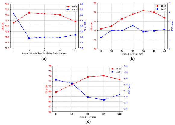
Figure 9: Effects of $k$-nearest neighbour in global feature space, mined view-set size, and mined view patch size. We report Dice and ASD of GLCon on the ACDC dataset at the 5% labeled ratio. All the experiments are run with three different random seeds.

Training Details of Competing CL Methods.   We identically follow the default setting in each CL framework [20, 83, 19, 37, 80] except the epochs number. We train each model in the semi-supervised setting. For labeled data, we follow the same training strategy in Section 3.1. As for unlabeled data, we strictly follow the default settings in each baseline. Specifically, for fair comparisons, we pre-train each CL baseline and our proposed CL pre-trained method (i.e., GLCon) for 100 epochs in all our experiments. Then we fine-tune each CL model with our proposed principles with the same setting, as provided in Appendix A. For $k$NN-MoCo [83], given the following ablation study we set the number of neighbors $k$ as 5, and further compare different settings of $k$ in $k$NN-MoCo [83] in the following subsection. All the experiments are run with three different random seeds, and the results we present are calculated from the validation set.

Comparisons with CL-based Frameworks.   Table 5 presents the comparisons between our proposed methods (i.e., GLCon and MONA) and various CL baselines. After analyzing these extensive results, we can draw several consistent observations. First, we can observe that our proposed GLCon achieves performance gains under all the labeled ratios, which not only demonstrates the effectiveness of our method, but also further verifies this argument using “global-local” strategy [14]. The average improvement in Dice obtained by GLCon could reach up to 2.53%, compared to the second best scores at different labeled ratios. Second, we can find that incorporating our proposed three principles significantly outperforms the CL baselines without fine-tuning, across all frameworks and different labeled ratios. These experimental findings suggest that our proposed three principles can further improve the generalization across different labeled ratios. On the ACDC dataset at the 1% labeled ratio, the backbones equipped with all three principles all obtain promising results, improving the performance of MoCov2, $k$NN-MoCo, SimCLR, BYOL, ISD, and our GLCon by 39.1%, 38.5%, 40.9%, 41.2%, 34.3%, 33.3%, respectively. The ACDC dataset is a popular multi-class medical image segmentation dataset, with massive imbalanced or long-tailed class distribution cases. The imbalanced or long-tailed class distribution gap could result in the vanilla models overfitting to the head class, and generalizing very poorly to the tail class. With the addition of under-sampling the head classes, the principle – tailness – can be deemed as the prominent strategy to yield better generalization and segmentation performance of the models across different labeled ratios. Similar results are found under 5% and 10% labeled ratios. Third, over a wide range of labeled ratios, MONA can establish the new state-of-the-art performance bar for semi-supervised 2D medical image segmentation. Particularly, MONA – for the first time – boots the segmentation performance with 10% labeled ratio over the fully-supervised method while significantly outperforming all the other semi-supervised methods by a large margin. In summary, our proposed methods (i.e., GLCon and MONA) obtain remarkable performance on all labeled settings. The results verify the superiority of our proposed three principles (i.e., tailness, consistency, diversity) jointly, which makes the model well generalize to different labeled settings, and can be easily and seamlessly plugged into all other CL frameworks [20, 83, 19, 37, 80] adopting the two-branch design, demonstrating that these concepts consistently help the model yield extra performance boosts for them all.

Figure 10: Effects of hyperparameters $\lambda_{1},\lambda_{2},\lambda_{3},\lambda_{4}$. We report Dice and ASD of MONA on the ACDC dataset at the 5% labeled ratio. All the experiments are run with three different random seeds.

Generalization Across CL Frameworks   As demonstrated in Table 6, incorporating tailness, consistency, and diversity have obviously superior performance boosts, which is aligned with consistent observations with Section 4.2 can be drawn. This suggests that these three principles can serve as desirable properties for medical image segmentation in both supervised and unsupervised settings.

Does $k$-nearest neighbour in global feature space help?   Prior work suggests that the use of stronger augmentations and nearest neighbour can be the very effective tools in learning additional invariances [83]. That is, both the specific number of nearest neighbours and specific augmentation strategies are necessary to achieve superior performance. In this subsection, we study the relationship of $k$-nearest neighbour in global feature space and the behavior of our GLCon for the downstream medical image segmentation. Here we first follow the same augmentation strategies in [83] (More analysis on data augmentation can be found in Section 4.2), and then conduct ablation studies on how the choices of $k$-nearest neighbour can influence the performance of GLCon. Specifically, we run GLCon on the ACDC dataset at the 5% labeled ratio with a range of $k\in\{3,5,7,10,12\}$. Figure 9(a) shows the ablation study on $k$-nearest neighbour in global feature on the segmentation performance. As is shown, we find that GLCon at $k=5,7,10$ have almost identical performance ($k=5$ has slightly better performance compared to other two settings), and all have superior performance compared to all others. In contrast, GLCon – through the use of randomly selected samples – is capable of finding diverse yet semantically consistent anatomical features from the entire dataset, which at the same time gives better segmentation performance.

Ablation Study of Mined View-Set Size.   We then conduct ablation studies on how the mined view-set size in GLCon can influence the segmentation performance. We run GLCon on the ACDC dataset at 5% labeled ratio with a range of the mined view-set size $\in\{12,18,24,30,36,42,48\}$. The results are summarized in Figure 9(b). As is shown, we find that GLCon trained with view-set size $36$ and $42$ have similar or superior performance compared to all other settings, and our model with view-set size of $36$ achieves the highest performance.

Ablation Study of Mined View Size.   Lastly, we study the influence of mined view size on the segmentation performance. Specifically, we run GLCon on the ACDC dataset at the 5% labeled ratio with a range of the mined view size $\in\{8,16,32,64,128\}$. Figure 9(c) shows the ablation study of mined view size on the segmentation performance. As is shown, we observe that GLCon trained with mined view size of $32$ and $64$ have similar segmentation abilities, and both achieve superior performance compared to other settings. Here the mined view size of $64$ works the best for GLCon to yield the superior segmentation performance.

Conclusion.   Given the above ablation study, we set $k$, mined view-set size, patch size as $5$, $36$, $64\times 64$ in our experiments, respectively. This can contribute to satisfactory segmentation performance.

Appendix E Ablation Study of Anatomical Contrastive Reconstruction

In this section, we give a detailed analysis on the choice of the parameters in the anatomical contrastive reconstruction fine-tuning, and take a deeper look and understand how they contribute to the final segmentation performance. All the hyperparameters in training are the same across three benchmark datasets. All the experiments are run with three different random seeds, and the experimental results we report are calculated from the validation set.

Ablation Study of Total Loss $\mathcal{L}_{\text{total}}$.   Proper choices of hyperparameters in total loss $\mathcal{L}_{\text{total}}$ (See Section 3.2) play a significant role in improving overall segmentation quality. We hence conduct the fine-grained analysis of the hyperparameters in $\mathcal{L}_{\text{total}}$. In practice, we fine-tune the models with three independent runs, and grid search to select multiple hyperparameters. Specifically, we run MONA on the ACDC dataset at the 5% labeled ratio with a range of different hyperparameters $\lambda_{1}\!\in\!\{0.005,0.001,0.05,0.01,0.05,0.1\}$, and $\lambda_{2},\lambda_{3},\lambda_{4}\!\in\!\{0.1,0.2,0.5,1.0,2.0,10.0\}$. We summarize the results in Figure 10, and take the best setting $\lambda_{1}\!=\!0.01$, $\lambda_{2}\!=\!1.0$, $\lambda_{3}\!=\!1.0,\lambda_{4}\!=\!1.0$.

Ablation Study of Confidence Threshold ${\delta_{\theta}}$.   We then assess the influence of ${\delta_{\theta}}$ on the segmentation performance. Specifically, we run MONA on the ACDC dataset at the 5% labeled ratio with a range of the confidence threshold ${\delta_{\theta}}\in\{0.85,0.88,0.91,0.94,0.97,1.0\}$. Figure 11(a) shows the ablation study of ${\delta_{\theta}}$ on the segmentation performance. As we can see, MONA on ${\delta_{\theta}}=0.97$ has superior performance compared to other settings.

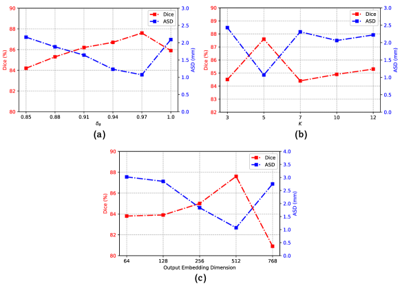
Figure 11: Effects of confidence threshold ${\delta_{\theta}}$, $K$-nearest neighbour constraint, and output embedding dimension. We report Dice and ASD of MONA on the ACDC dataset at the 5% labeled ratio. All the experiments are run with three different random seeds.

Ablation Study of $K$-Nearest Neighbour Constraint.   Next, we conduct ablation studies on how the choices of $K$ in $K$-nearest neighbour constraint can influence the segmentation performance. Specifically, we run MONA on the ACDC dataset at the 5% labeled ratio with a range of the choices $K\in\{3,5,7,10,12\}$. Figure 11(b) shows the ablation study of $K$ choices on the segmentation performance. As we can see, MONA on $K=5$ achieves the best performance compared to other settings.

Ablation Study of Output Embedding Dimension.   Finally, we study the influence of the output embedding dimension on the segmentation performance of MONA. Specifically, we run MONA on the ACDC dataset at the 5% labeled ratio with a range of output embedding dimension $\in\{64,128,256,512,768\}$. Figure 11(c) shows the ablation study of output embedding dimension on the segmentation performance. As we can see, MONA with output embedding dimension of $512$, can be trained to outperform other settings.

Conclusion.   Given the above ablation study, we select $\lambda_{1}\!=\!0.01$, $\lambda_{2}\!=\!1.0$, $\lambda_{3}\!=\!1.0,\lambda_{4}\!=\!1.0$, ${\delta_{\theta}}=0.97$, $K=5$, output embedding dimension $=512$ in our experiments. This can provide the optimal segmentation performance across different labeled ratios.

References

- [1] Md Zahangir Alom, Mahmudul Hasan, Chris Yakopcic, Tarek M Taha, and Vijayan K Asari. Recurrent residual convolutional neural network based on U-Net (R2U-Net) for medical image segmentation. arXiv preprint arXiv:1802.06955, 2018.
- [2] Sanjeev Arora, Hrishikesh Khandeparkar, Mikhail Khodak, Orestis Plevrakis, and Nikunj Saunshi. A theoretical analysis of contrastive unsupervised representation learning. arXiv preprint arXiv:1902.09229, 2019.
- [3] Mehdi Azabou, Mohammad Gheshlaghi Azar, Ran Liu, Chi-Heng Lin, Erik C Johnson, Kiran Bhaskaran-Nair, Max Dabagia, Bernardo Avila-Pires, Lindsey Kitchell, Keith B Hengen, et al. Mine your own view: Self-supervised learning through across-sample prediction. arXiv preprint arXiv:2102.10106, 2021.
- [4] Wenjia Bai, Ozan Oktay, Matthew Sinclair, Hideaki Suzuki, Martin Rajchl, Giacomo Tarroni, Ben Glocker, Andrew King, Paul M Matthews, and Daniel Rueckert. Semi-supervised learning for network-based cardiac mr image segmentation. In MICCAI, 2017.
- [5] Peter L Bartlett and Shahar Mendelson. Rademacher and gaussian complexities: Risk bounds and structural results. Journal of Machine Learning Research, 3(Nov):463–482, 2002.
- [6] Olivier Bernard, Alain Lalande, Clement Zotti, Frederick Cervenansky, Xin Yang, Pheng-Ann Heng, Irem Cetin, Karim Lekadir, Oscar Camara, Miguel Angel Gonzalez Ballester, et al. Deep learning techniques for automatic MRI cardiac multi-structures segmentation and diagnosis: Is the problem solved? IEEE Transactions on Medical Imaging, 2018.
- [7] Patrick Bilic, Patrick Ferdinand Christ, Eugene Vorontsov, Grzegorz Chlebus, Hao Chen, Qi Dou, Chi-Wing Fu, Xiao Han, Pheng-Ann Heng, Jürgen Hesser, et al. The liver tumor segmentation benchmark (lits). arXiv preprint arXiv:1901.04056, 2019.
- [8] Charles Blundell, Julien Cornebise, Koray Kavukcuoglu, and Daan Wierstra. Weight uncertainty in neural network. In ICML, 2015.
- [9] Gerda Bortsova, Florian Dubost, Laurens Hogeweg, Ioannis Katramados, and Marleen de Bruijne. Semi-supervised medical image segmentation via learning consistency under transformations. In MICCAI, 2019.
- [10] Robin Camarasa, Daniel Bos, Jeroen Hendrikse, Paul Nederkoorn, Eline Kooi, Aad van der Lugt, and Marleen de Bruijne. Quantitative comparison of monte-carlo dropout uncertainty measures for multi-class segmentation. In Uncertainty for Safe Utilization of Machine Learning in Medical Imaging, and Graphs in Biomedical Image Analysis. 2020.
- [11] Hu Cao, Yueyue Wang, Joy Chen, Dongsheng Jiang, Xiaopeng Zhang, Qi Tian, and Manning Wang. Swin-unet: Unet-like pure transformer for medical image segmentation. arXiv preprint arXiv:2105.05537, 2021.
- [12] Xuyang Cao, Houjin Chen, Yanfeng Li, Yahui Peng, Shu Wang, and Lin Cheng. Uncertainty aware temporal-ensembling model for semi-supervised abus mass segmentation. IEEE Transactions on Medical Imaging, 2020.
- [13] Mathilde Caron, Ishan Misra, Julien Mairal, Priya Goyal, Piotr Bojanowski, and Armand Joulin. Unsupervised learning of visual features by contrasting cluster assignments. In NeurIPS, 2020.
- [14] Krishna Chaitanya, Ertunc Erdil, Neerav Karani, and Ender Konukoglu. Contrastive learning of global and local features for medical image segmentation with limited annotations. In NeurIPS, 2020.
- [15] Krishna Chaitanya, Ertunc Erdil, Neerav Karani, and Ender Konukoglu. Local contrastive loss with pseudo-label based self-training for semi-supervised medical image segmentation. arXiv preprint arXiv:2112.09645, 2021.
- [16] Jieneng Chen, Yongyi Lu, Qihang Yu, Xiangde Luo, Ehsan Adeli, Yan Wang, Le Lu, Alan L Yuille, and Yuyin Zhou. Transunet: Transformers make strong encoders for medical image segmentation. In MICCAI, 2021.
- [17] Liang-Chieh Chen, George Papandreou, Iasonas Kokkinos, Kevin Murphy, and Alan L Yuille. Deeplab: Semantic image segmentation with deep convolutional nets, atrous convolution, and fully connected crfs. IEEE transactions on pattern analysis and machine intelligence, 2017.
- [18] Liang-Chieh Chen, Yukun Zhu, George Papandreou, Florian Schroff, and Hartwig Adam. Encoder-decoder with atrous separable convolution for semantic image segmentation. In ECCV, 2018.
- [19] Ting Chen, Simon Kornblith, Mohammad Norouzi, and Geoffrey Hinton. A simple framework for contrastive learning of visual representations. In ICML, 2020.
- [20] Xinlei Chen, Haoqi Fan, Ross Girshick, and Kaiming He. Improved baselines with momentum contrastive learning. arXiv preprint arXiv:2003.04297, 2020.
- [21] Xiaokang Chen, Yuhui Yuan, Gang Zeng, and Jingdong Wang. Semi-supervised semantic segmentation with cross pseudo supervision. In CVPR, 2021.
- [22] Ching-Yao Chuang, Joshua Robinson, Yen-Chen Lin, Antonio Torralba, and Stefanie Jegelka. Debiased contrastive learning. In NeurIPS, 2020.
- [23] Wenhui Cui, Yanlin Liu, Yuxing Li, Menghao Guo, Yiming Li, Xiuli Li, Tianle Wang, Xiangzhu Zeng, and Chuyang Ye. Semi-supervised brain lesion segmentation with an adapted mean teacher model. In MICCAI, 2019.
- [24] Yin Cui, Menglin Jia, Tsung-Yi Lin, Yang Song, and Serge Belongie. Class-balanced loss based on effective number of samples. In CVPR, 2019.
- [25] Jifeng Dai, Haozhi Qi, Yuwen Xiong, Yi Li, Guodong Zhang, Han Hu, and Yichen Wei. Deformable convolutional networks. In CVPR, 2017.
- [26] Aditya Desai, Zhaozhuo Xu, Menal Gupta, Anu Chandran, Antoine Vial-Aussavy, and Anshumali Shrivastava. Raw nav-merge seismic data to subsurface properties with mlp based multi-modal information unscrambler. In NeurIPS, 2021.
- [27] Alexey Dosovitskiy, Lucas Beyer, Alexander Kolesnikov, Dirk Weissenborn, Xiaohua Zhai, Thomas Unterthiner, Mostafa Dehghani, Matthias Minderer, Georg Heigold, Sylvain Gelly, et al. An image is worth 16x16 words: Transformers for image recognition at scale. In ICLR, 2020.
- [28] Deng-Ping Fan, Tao Zhou, Ge-Peng Ji, Yi Zhou, Geng Chen, Huazhu Fu, Jianbing Shen, and Ling Shao. Inf-net: Automatic covid-19 lung infection segmentation from ct images. IEEE Transactions on Medical Imaging, 2020.
- [29] Kang Fang and Wu-Jun Li. Dmnet: difference minimization network for semi-supervised segmentation in medical images. In MICCAI, 2020.
- [30] Gaurav Fotedar, Nima Tajbakhsh, Shilpa Ananth, and Xiaowei Ding. Extreme consistency: Overcoming annotation scarcity and domain shifts. In MICCAI, 2020.
- [31] Geoff French, Samuli Laine, Timo Aila, Michal Mackiewicz, and Graham Finlayson. Semi-supervised semantic segmentation needs strong, varied perturbations. In BMVC, 2020.
- [32] Tommaso Furlanello, Zachary Lipton, Michael Tschannen, Laurent Itti, and Anima Anandkumar. Born again neural networks. In International Conference on Machine Learning, pages 1607–1616. PMLR, 2018.
- [33] Yarin Gal and Zoubin Ghahramani. Dropout as a bayesian approximation: Representing model uncertainty in deep learning. In ICML, 2016.
- [34] Adrian Galdran, Gustavo Carneiro, and Miguel A González Ballester. Balanced-mixup for highly imbalanced medical image classification. In MICCAI, 2021.
- [35] Simon Graham, Hao Chen, Jevgenij Gamper, Qi Dou, Pheng-Ann Heng, David Snead, Yee Wah Tsang, and Nasir Rajpoot. Mild-net: Minimal information loss dilated network for gland instance segmentation in colon histology images. Medical image analysis, 2019.
- [36] Yves Grandvalet and Yoshua Bengio. Semi-supervised learning by entropy minimization. NeurIPS, 2004.
- [37] Jean-Bastien Grill, Florian Strub, Florent Altché, Corentin Tallec, Pierre Richemond, Elena Buchatskaya, Carl Doersch, Bernardo Avila Pires, Zhaohan Guo, Mohammad Gheshlaghi Azar, et al. Bootstrap your own latent-a new approach to self-supervised learning. In NeurIPS, 2020.
- [38] Raia Hadsell, Sumit Chopra, and Yann LeCun. Dimensionality reduction by learning an invariant mapping. In CVPR, 2006.
- [39] Ali Hatamizadeh, Yucheng Tang, Vishwesh Nath, Dong Yang, Andriy Myronenko, Bennett Landman, Holger Roth, and Daguang Xu. Unetr: Transformers for 3d medical image segmentation. arXiv preprint arXiv:2103.10504, 2021.
- [40] Kaiming He, Haoqi Fan, Yuxin Wu, Saining Xie, and Ross Girshick. Momentum contrast for unsupervised visual representation learning. In CVPR, 2020.
- [41] Kaiming He, Xiangyu Zhang, Shaoqing Ren, and Jian Sun. Deep residual learning for image recognition. In CVPR, 2016.
- [42] R Devon Hjelm, Alex Fedorov, Samuel Lavoie-Marchildon, Karan Grewal, Phil Bachman, Adam Trischler, and Yoshua Bengio. Learning deep representations by mutual information estimation and maximization. In ICLR, 2019.
- [43] Xinrong Hu, Dewen Zeng, Xiaowei Xu, and Yiyu Shi. Semi-supervised contrastive learning for label-efficient medical image segmentation. In MICCAI, 2021.
- [44] Fabian Isensee, Paul F Jaeger, Simon AA Kohl, Jens Petersen, and Klaus H Maier-Hein. nnu-net: a self-configuring method for deep learning-based biomedical image segmentation. Nature methods, 2021.
- [45] Ziyu Jiang, Tianlong Chen, Ting Chen, and Zhangyang Wang. Improving contrastive learning on imbalanced data via open-world sampling. In NeurIPS, 2021.
- [46] Alain Jungo and Mauricio Reyes. Assessing reliability and challenges of uncertainty estimations for medical image segmentation. In MICCAI, 2019.
- [47] Bingyi Kang, Yu Li, Sa Xie, Zehuan Yuan, and Jiashi Feng. Exploring balanced feature spaces for representation learning. In ICLR, 2020.
- [48] Alex Kendall and Yarin Gal. What uncertainties do we need in bayesian deep learning for computer vision? In NeurIPS, 2017.
- [49] Dong-Hyun Lee et al. Pseudo-label: The simple and efficient semi-supervised learning method for deep neural networks. In Workshop on challenges in representation learning, ICML, 2013.
- [50] Jun Li, Quan Quan, and S Kevin Zhou. Mixcl: Pixel label matters to contrastive learning. arXiv preprint arXiv:2203.02114, 2022.
- [51] Junnan Li, Pan Zhou, Caiming Xiong, and Steven Hoi. Prototypical contrastive learning of unsupervised representations. In ICLR, 2021.
- [52] Shuailin Li, Chuyu Zhang, and Xuming He. Shape-aware semi-supervised 3d semantic segmentation for medical images. In MICCAI, 2020.
- [53] Xiaomeng Li, Hao Chen, Xiaojuan Qi, Qi Dou, Chi-Wing Fu, and Pheng-Ann Heng. H-denseunet: hybrid densely connected unet for liver and tumor segmentation from ct volumes. IEEE Trans. Med. Imaging, 2018.
- [54] Xiaomeng Li, Lequan Yu, Hao Chen, Chi-Wing Fu, Lei Xing, and Pheng-Ann Heng. Transformation-consistent self-ensembling model for semisupervised medical image segmentation. IEEE Transactions on Neural Networks and Learning Systems, 2020.
- [55] Tsung-Yi Lin, Piotr Dollár, Ross Girshick, Kaiming He, Bharath Hariharan, and Serge Belongie. Feature pyramid networks for object detection. In CVPR, 2017.
- [56] Tsung-Yi Lin, Priya Goyal, Ross Girshick, Kaiming He, and Piotr Dollár. Focal loss for dense object detection. In ICCV, 2017.
- [57] Shikun Liu, Shuaifeng Zhi, Edward Johns, and Andrew J Davison. Bootstrapping semantic segmentation with regional contrast. arXiv preprint arXiv:2104.04465, 2021.
- [58] Jonathan Long, Evan Shelhamer, and Trevor Darrell. Fully convolutional networks for semantic segmentation. In CVPR, 2015.
- [59] Xiangde Luo, Wenjun Liao, Jieneng Chen, Tao Song, Yinan Chen, Shichuan Zhang, Nianyong Chen, Guotai Wang, and Shaoting Zhang. Efficient semi-supervised gross target volume of nasopharyngeal carcinoma segmentation via uncertainty rectified pyramid consistency. In MICCAI, 2021.
- [60] Alireza Mehrtash, William M Wells, Clare M Tempany, Purang Abolmaesumi, and Tina Kapur. Confidence calibration and predictive uncertainty estimation for deep medical image segmentation. IEEE transactions on medical imaging, 2020.
- [61] Fausto Milletari, Nassir Navab, and Seyed-Ahmad Ahmadi. V-net: Fully convolutional neural networks for volumetric medical image segmentation. In 3DV. IEEE, 2016.
- [62] Hossein Mobahi, Mehrdad Farajtabar, and Peter Bartlett. Self-distillation amplifies regularization in hilbert space. Advances in Neural Information Processing Systems, 33:3351–3361, 2020.
- [63] Tanya Nair, Doina Precup, Douglas L Arnold, and Tal Arbel. Exploring uncertainty measures in deep networks for multiple sclerosis lesion detection and segmentation. Medical image analysis, 2020.
- [64] Dong Nie, Yaozong Gao, Li Wang, and Dinggang Shen. Asdnet: Attention based semi-supervised deep networks for medical image segmentation. In MICCAI, 2018.
- [65] Ozan Oktay, Jo Schlemper, Loic Le Folgoc, Matthew Lee, Mattias Heinrich, Kazunari Misawa, Kensaku Mori, Steven McDonagh, Nils Y Hammerla, Bernhard Kainz, et al. Attention u-net: Learning where to look for the pancreas. arXiv preprint arXiv:1804.03999, 2018.
- [66] Aaron van den Oord, Yazhe Li, and Oriol Vinyals. Representation learning with contrastive predictive coding. arXiv preprint arXiv:1807.03748, 2018.
- [67] Yassine Ouali, Céline Hudelot, and Myriam Tami. Semi-supervised semantic segmentation with cross-consistency training. In CVPR, 2020.
- [68] Adam Paszke, Sam Gross, Francisco Massa, Adam Lerer, James Bradbury, Gregory Chanan, Trevor Killeen, Zeming Lin, Natalia Gimelshein, Luca Antiga, et al. Pytorch: An imperative style, high-performance deep learning library. In NeurIPS, 2019.
- [69] Fábio Perez, Cristina Vasconcelos, Sandra Avila, and Eduardo Valle. Data augmentation for skin lesion analysis. In OR 2.0 Context-Aware Operating Theaters, Computer Assisted Robotic Endoscopy, Clinical Image-Based Procedures, and Skin Image Analysis, pages 303–311. Springer, 2018.
- [70] Siyuan Qiao, Wei Shen, Zhishuai Zhang, Bo Wang, and Alan Yuille. Deep co-training for semi-supervised image recognition. In ECCV, 2018.
- [71] Quan Quan, Qingsong Yao, Jun Li, et al. Information-guided pixel augmentation for pixel-wise contrastive learning. arXiv preprint arXiv:2211.07118, 2022.
- [72] Simon Reiß, Constantin Seibold, Alexander Freytag, Erik Rodner, and Rainer Stiefelhagen. Every annotation counts: Multi-label deep supervision for medical image segmentation. In CVPR, 2021.
- [73] Olaf Ronneberger, Philipp Fischer, and Thomas Brox. U-net: Convolutional networks for biomedical image segmentation. In MICCAI, 2015.
- [74] Abhijit Guha Roy, Jie Ren, Shekoofeh Azizi, Aaron Loh, Vivek Natarajan, Basil Mustafa, Nick Pawlowski, Jan Freyberg, Yuan Liu, Zach Beaver, et al. Does your dermatology classifier know what it doesn’t know? detecting the long-tail of unseen conditions. Medical Image Analysis, 2022.
- [75] Mehdi Sajjadi, Mehran Javanmardi, and Tolga Tasdizen. Regularization with stochastic transformations and perturbations for deep semi-supervised learning. In NeurIPS, 2016.
- [76] Gonglei Shi, Li Xiao, Yang Chen, and S Kevin Zhou. Marginal loss and exclusion loss for partially supervised multi-organ segmentation. Medical Image Analysis, 2021.
- [77] Karen Simonyan and Andrew Zisserman. Very deep convolutional networks for large-scale image recognition. arXiv preprint arXiv:1409.1556, 2014.
- [78] Kihyuk Sohn, David Berthelot, Nicholas Carlini, Zizhao Zhang, Han Zhang, Colin A Raffel, Ekin Dogus Cubuk, Alexey Kurakin, and Chun-Liang Li. Fixmatch: Simplifying semi-supervised learning with consistency and confidence. NeurIPS, 2020.
- [79] Antti Tarvainen and Harri Valpola. Mean teachers are better role models: Weight-averaged consistency targets improve semi-supervised deep learning results. In NeurIPS, 2017.
- [80] Ajinkya Tejankar, Soroush Abbasi Koohpayegani, Vipin Pillai, Paolo Favaro, and Hamed Pirsiavash. Isd: Self-supervised learning by iterative similarity distillation. In ICCV, 2021.
- [81] Jeya Maria Jose Valanarasu, Poojan Oza, Ilker Hacihaliloglu, and Vishal M Patel. Medical transformer: Gated axial-attention for medical image segmentation. In MICCAI, 2021.
- [82] Gabriele Valvano, Andrea Leo, and Sotirios A Tsaftaris. Learning to segment from scribbles using multi-scale adversarial attention gates. IEEE Transactions on Medical Imaging, 2021.
- [83] Wouter Van Gansbeke, Simon Vandenhende, Stamatios Georgoulis, and Luc V Gool. Revisiting contrastive methods for unsupervised learning of visual representations. In NeurIPS, 2021.
- [84] Ashish Vaswani, Noam Shazeer, Niki Parmar, Jakob Uszkoreit, Llion Jones, Aidan N Gomez, Łukasz Kaiser, and Illia Polosukhin. Attention is all you need. In NeurIPS, 2017.
- [85] Vikas Verma, Kenji Kawaguchi, Alex Lamb, Juho Kannala, Yoshua Bengio, and David Lopez-Paz. Interpolation consistency training for semi-supervised learning. In IJCAI, 2019.
- [86] Tuan-Hung Vu, Himalaya Jain, Maxime Bucher, Matthieu Cord, and Patrick Pérez. Advent: Adversarial entropy minimization for domain adaptation in semantic segmentation. In CVPR, 2019.
- [87] Yicheng Wu, Yong Xia, Yang Song, Donghao Zhang, Dongnan Liu, Chaoyi Zhang, and Weidong Cai. Vessel-net: retinal vessel segmentation under multi-path supervision. In MICCAI, 2019.
- [88] Yicheng Wu, Yong Xia, Yang Song, Yanning Zhang, and Weidong Cai. Multiscale network followed network model for retinal vessel segmentation. In MICCAI, 2018.
- [89] Zhirong Wu, Yuanjun Xiong, X Yu Stella, and Dahua Lin. Unsupervised feature learning via non-parametric instance discrimination. In CVPR, 2018.
- [90] Qizhe Xie, Minh-Thang Luong, Eduard Hovy, and Quoc V Le. Self-training with noisy student improves imagenet classification. In CVPR, 2020.
- [91] Yutong Xie, Jianpeng Zhang, Chunhua Shen, and Yong Xia. Cotr: Efficiently bridging cnn and transformer for 3d medical image segmentation. In MICCAI, 2021.
- [92] Yuan Xue, Hui Tang, Zhi Qiao, Guanzhong Gong, Yong Yin, Zhen Qian, Chao Huang, Wei Fan, and Xiaolei Huang. Shape-aware organ segmentation by predicting signed distance maps. arXiv preprint arXiv:1912.03849, 2019.
- [93] Ke Yan, Jinzheng Cai, Dakai Jin, Shun Miao, Dazhou Guo, Adam P Harrison, Youbao Tang, Jing Xiao, Jingjing Lu, and Le Lu. Sam: Self-supervised learning of pixel-wise anatomical embeddings in radiological images. IEEE Trans. Med. Imaging, 2022.
- [94] Yuzhe Yang and Zhi Xu. Rethinking the value of labels for improving class-imbalanced learning. In NeurIPS, 2020.
- [95] Chenyu You, Ruihan Zhao, Fenglin Liu, Sandeep Chinchali, Ufuk Topcu, Lawrence Staib, and James S Duncan. Class-aware generative adversarial transformers for medical image segmentation. arXiv preprint arXiv:2201.10737, 2022.
- [96] Chenyu You, Ruihan Zhao, Lawrence Staib, and James S Duncan. Momentum contrastive voxel-wise representation learning for semi-supervised volumetric medical image segmentation. arXiv preprint arXiv:2105.07059, 2021.
- [97] Chenyu You, Yuan Zhou, Ruihan Zhao, Lawrence Staib, and James S Duncan. Simcvd: Simple contrastive voxel-wise representation distillation for semi-supervised medical image segmentation. IEEE Transactions on Medical Imaging, 2022.
- [98] Lequan Yu, Shujun Wang, Xiaomeng Li, Chi-Wing Fu, and Pheng-Ann Heng. Uncertainty-aware self-ensembling model for semi-supervised 3d left atrium segmentation. In MICCAI, 2019.
- [99] Yu Zeng, Yunzhi Zhuge, Huchuan Lu, and Lihe Zhang. Joint learning of saliency detection and weakly supervised semantic segmentation. In ICCV, 2019.
- [100] Yizhe Zhang, Lin Yang, Jianxu Chen, Maridel Fredericksen, David P Hughes, and Danny Z Chen. Deep adversarial networks for biomedical image segmentation utilizing unannotated images. In MICCAI, 2017.
- [101] Zhilu Zhang and Mert Sabuncu. Self-distillation as instance-specific label smoothing. Advances in Neural Information Processing Systems, 33:2184–2195, 2020.
- [102] Zizhao Zhang, Lin Yang, and Yefeng Zheng. Translating and segmenting multimodal medical volumes with cycle-and shape-consistency generative adversarial network. In CVPR, 2018.
- [103] Ziyuan Zhao, Fangcheng Zhou, Zeng Zeng, Cuntai Guan, and S Kevin Zhou. Meta-hallucinator: Towards few-shot cross-modality cardiac image segmentation. In Medical Image Computing and Computer Assisted Intervention–MICCAI 2022: 25th International Conference, Singapore, September 18–22, 2022, Proceedings, Part V, pages 128–139. Springer, 2022.
- [104] Han Zheng, Lanfen Lin, Hongjie Hu, Qiaowei Zhang, Qingqing Chen, Yutaro Iwamoto, Xianhua Han, Yen-Wei Chen, Ruofeng Tong, and Jian Wu. Semi-supervised segmentation of liver using adversarial learning with deep atlas prior. In MICCAI, 2019.
- [105] Mingkai Zheng, Shan You, Fei Wang, Chen Qian, Changshui Zhang, Xiaogang Wang, and Chang Xu. Ressl: Relational self-supervised learning with weak augmentation. In NeurIPS, 2021.
- [106] Yuyin Zhou, Yan Wang, Peng Tang, Song Bai, Wei Shen, Elliot Fishman, and Alan Yuille. Semi-supervised 3d abdominal multi-organ segmentation via deep multi-planar co-training. In WACV, 2019.
- [107] Xiangxin Zhu, Dragomir Anguelov, and Deva Ramanan. Capturing long-tail distributions of object subcategories. In CVPR, 2014.
- [108] Xiahai Zhuang and Juan Shen. Multi-scale patch and multi-modality atlases for whole heart segmentation of mri. Medical image analysis, 2016.