3D non-LTE iron abundances in FG-type dwarfs

Iron is one of the most important elements in stellar astrophysics. However, spectroscopic measurements of its abundance are prone to systematic modelling errors. We present three dimensional non-local thermodynamic equilibrium (3D non-LTE) calculations across $32$ STAGGER-grid models with effective temperatures from $5000\,\mathrm{K}$ to $6500\,\mathrm{K}$, surface gravities of $4.0\,\mathrm{dex}$ and $4.5\,\mathrm{dex}$, and metallicities from $-3\,\mathrm{dex}$ to $0\,\mathrm{dex}$, and we study the effects on $171$ Fe I and $12$ Fe II optical lines. In warm metal-poor stars, the 3D non-LTE abundances are up to $0.5\,\mathrm{dex}$ larger than 1D LTE abundances inferred from Fe I lines of an intermediate excitation potential. In contrast, the 3D non-LTE abundances can be $0.2\,\mathrm{dex}$ smaller in cool metal-poor stars when using Fe I lines of a low excitation potential. The corresponding abundance differences between 3D non-LTE and 1D non-LTE are generally less severe but can still reach $\pm 0.2\,\mathrm{dex}$. For Fe II lines, the 3D abundances range from up to $0.15\,\mathrm{dex}$ larger to $0.10\,\mathrm{dex}$ smaller than 1D abundances, with negligible departures from 3D LTE except for the warmest stars at the lowest metallicities. The results were used to correct 1D LTE abundances of the Sun and Procyon (HD 61421), and of the metal-poor stars HD 84937 and HD 140283, using an interpolation routine based on neural networks. The 3D non-LTE models achieve an improved ionisation balance in all four stars. In the two metal-poor stars, they removed excitation imbalances amounting to $250\,\mathrm{K}$ to $300\,\mathrm{K}$ errors in effective temperature. For Procyon, the 3D non-LTE models suggest $\mathrm{\left[Fe/H\right]}=0.11\pm 0.03$, which is significantly larger than literature values based on simpler models. We make the 3D non-LTE interpolation routine for FG-type dwarfs publicly available, in addition to 1D non-LTE departure coefficients for standard MARCS models of FGKM-type dwarfs and giants. These tools, together with an extended 3D LTE grid for Fe II from 2019, can help improve the accuracy of stellar parameter and iron abundance determinations for late-type stars.

1 Introduction

Iron is one of the most discussed elements in astrophysics. It is the seventh most abundant element in the Sun (Asplund et al., 2021) and an important source of opacity throughout the solar interior (Bailey et al., 2015; Mondet et al., 2015). Its high cosmic abundance and open $3d$ shell conspire to make iron dominate the spectra of FG-type dwarfs such as the Sun, and so it is the usual proxy of the stellar metal mass fraction ($Z$). It is also a precise and illuminating tracer of the evolution of galaxies, being formed copiously by both core-collapse supernovae on short timescales, and Type Ia supernovae at later cosmic epochs (Maoz & Graur, 2017). In spectroscopic surveys, including extremely large ones such as APOGEE (Ahumada et al., 2020) and GALAH (Buder et al., 2021), iron is often used to infer other fundamental stellar parameters such as the effective temperature ($T_{\mathrm{eff}}$) and surface gravity ($\log{g}$), via excitation and ionisation equilibria of Fe I and Fe II lines (Frebel et al., 2013; Ruchti et al., 2013; Tsantaki et al., 2013; Ezzeddine et al., 2017; Li & Ezzeddine, 2022).

However, measurements of iron abundances ($A\left({\mathrm{Fe}}\right)$ or $\mathrm{\left[Fe/H\right]}$) can suffer from systematic modelling errors. Most spectroscopic analyses carried out today do the following: a) employ one-dimensional (1D) hydrostatic model stellar atmospheres that are necessarily in radiative equilibrium at the upper boundary; and b) invoke the assumption of local thermodynamic equilibrium (LTE). Both assumptions can alter Fe I and Fe II line strengths (Shchukina & Trujillo Bueno, 2001; Holzreuter & Solanki, 2012, 2013). The quantitative 1D LTE systematic errors typically depend on the excitation potential ($E_{\text{low}}$), and are different for Fe I and Fe II. Thus they may introduce errors in spectroscopic determinations of $T_{\mathrm{eff}}$ and $\log{g}$ as well.

The 1D LTE systematic errors are particularly prominent for warm, metal-poor stars, where $A\left({\mathrm{Fe}}\right)$ determinations are usually underestimated (Amarsi et al., 2016; Nordlander et al., 2017). Here, the reduced metal opacity results in a larger UV flux escaping the deeper photosphere, which drives a severe over-ionisation of Fe I and a slight over-excitation of Fe II (Shchukina et al., 2005). This non-LTE effect is enhanced by the steeper temperature gradients within metal-poor 3D model stellar atmospheres as efficient adiabatic cooling makes them much cooler in the upper layers than what is expected from 1D models that are close to radiative equilibrium (Collet et al., 2006, 2011).

In the last decade, 3D model stellar atmospheres combined with 3D non-LTE post-processing radiative transfer calculations have increasingly been used for spectroscopic abundance determinations of different elements. For iron this approach has not been utilised much, other than in studies of the Sun (Lind et al., 2017; Asplund et al., 2021) and of a small number of metal-poor stars (Amarsi et al., 2016; Nordlander et al., 2017).

Here we describe recent 3D non-LTE calculations for iron for FG-type dwarfs (Sect. 2). To our knowledge, this is the first grid of its kind. We briefly explore the systematic effects on 1D LTE and 1D non-LTE measurements of $A\left({\mathrm{Fe}}\right)$ across parameter space (Sect. 3), focussing on the $171$ Fe I and $12$ Fe II optical lines used in the analysis of the Gaia benchmark stars (GBS; Jofré et al. 2014). We present a routine based on neural networks that interpolates the predicted abundance differences (Sect. 4), and we describe the impact on four standard stars: the Sun, Procyon (HD 61421), HD 84937, and HD 140283 (Sect. 5). We end with a summary of our overall conclusions, and provide grids of 1D non-LTE departure coefficients for FGKM-type dwarfs and giants as well as the interpolation routine for 1D LTE versus 3D non-LTE abundance differences which is publicly available (Sect. 6).

2 Method

Table 1: Inelastic collision cross sections included in the model atom.

Process	Equation	Method	Ref.
Electron impact excitation	$\mathrm{{Fe\textsc{I}}}(i)+\mathrm{e^{-}}\leftrightarrow\mathrm{{Fe\textsc{I}}}(j)+\mathrm{e^{-}}$	$B$-spline $R$-matrix	a
	$\mathrm{{Fe\textsc{II}}}(i)+\mathrm{e^{-}}\leftrightarrow\mathrm{{Fe\textsc{II}}}(j)+\mathrm{e^{-}}$	$R$-matrix	b, c
Electron impact ionisation	$\mathrm{{Fe\textsc{I}}}(i)+\mathrm{e^{-}}\leftrightarrow\mathrm{{Fe\textsc{II}}}(j)+2\mathrm{e^{-}}$	Semi-empirical	d
	$\mathrm{{Fe\textsc{II}}}(i)+\mathrm{e^{-}}\leftrightarrow\mathrm{{Fe\textsc{III}}}(j)+2\mathrm{e^{-}}$
Hydrogen impact excitation	$\mathrm{{Fe\textsc{I}}}(i)+\mathrm{H(n=1)}\leftrightarrow\mathrm{{Fe\textsc{I}}}(j)+\mathrm{H(n=1)}$	Asymptotic model (LCAO)	e
		Free electron model	f
	$\mathrm{{Fe\textsc{II}}}(i)+\mathrm{H(n=1)}\leftrightarrow\mathrm{{Fe\textsc{II}}}(j)+\mathrm{H(n=1)}$	Asymptotic model (Simplified)	g
		Drawin	h
Charge transfer	$\mathrm{{Fe\textsc{I}}}(i)+\mathrm{H(n=1)}\leftrightarrow\mathrm{{Fe\textsc{II}}}(j)+\mathrm{H^{-}}$	Asymptotic model (LCAO)	e
	$\mathrm{{Fe\textsc{II}}}(i)+\mathrm{H(n=1)}\rightarrow\mathrm{{Fe\textsc{III}}}(j)+\mathrm{H^{-}}$	Asymptotic model (Simplified)	g

(a) Wang et al. (2018); (b) Bautista et al. (2015); (c) Zhang & Pradhan (1995); (d) Allen (1973); (e) Barklem (2018); (f) Kaulakys (1991); (g) Yakovleva et al. (2019); (h) Lambert (1993)

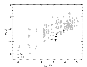
Figure 1: $E_{\text{low}}$ and $\log{gf}$ for the Jofré et al. (2014) set of Fe I and Fe II lines considered in this study.

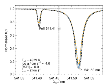
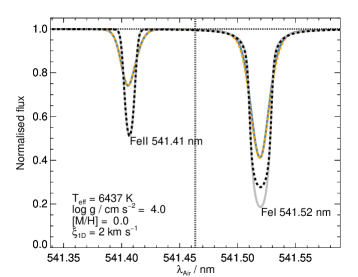
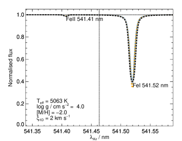
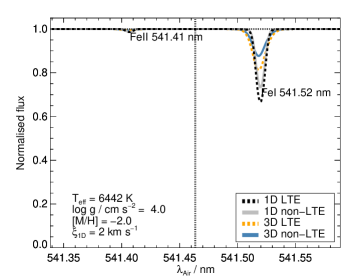
Figure 2: Synthetic spectra in LTE (dashed) and non-LTE (solid) from 1D ATMO and 3D STAGGER models with different $T_{\mathrm{eff}}$ (columns) and $\mathrm{\left[M/H\right]}$ (rows). The 1D spectra shown here were calculated with $\xi_{\text{mic;1D}}=2\,\mathrm{km\,s^{-1}}$ and without any macroturbulent broadening. An integration limit is illustrated as a vertical dashed line.

2.1 Model stellar atmospheres

Post-processing radiative transfer calculations were performed across a subset of the STAGGER grid of 3D hydrodynamic model stellar atmospheres (Magic et al., 2013). The selected models have four values of $T_{\mathrm{eff}}$ between $5000\,\mathrm{K}$ and $6500\,\mathrm{K}$, two values of $\log{g}$ of $4.0\,\mathrm{dex}$ and $4.5\,\mathrm{dex}$ (in units of logarithmic $\mathrm{cm\,s^{-2}}$), and four values of $\mathrm{\left[Fe/H\right]}$ between $-3.0\,\mathrm{dex}$ and $0.0\,\mathrm{dex}$. The models were computed with the solar chemical composition of Asplund et al. (2009), scaled by $\mathrm{\left[Fe/H\right]}$, and with an enhancement to the canonical $\upalpha$ elements (O, Ne, Mg, Si, S, Ar, Ca, and Ti) of $+0.4\,\mathrm{dex}$ for $\mathrm{\left[Fe/H\right]}\leq-1.0$. To avoid confusion in the subsequent discussion, $\mathrm{\left[M/H\right]}$ is used in place of $\mathrm{\left[Fe/H\right]}$ to represent the overall metallicity of the model stellar atmospheres.

Prior to carrying out the calculations in this work, the models were trimmed and re-gridded to both reduce the horizontal resolution (to speed up the calculations), and to increase the resolution in the steep continuum-forming regions (to improve accuracy), in the manner described in Sect. 2.1.1 of Amarsi et al. (2018). The calculations were carried out on five snapshots of each model.

Post-processing radiative transfer calculations were also performed on two families of 1D hydrostatic model stellar atmospheres: ATMO models (Magic et al. 2013, Appendix A) and an extended grid of MARCS models (Gustafsson et al., 2008). The ATMO models adopt the same equation of state, raw opacity data, opacity bins, and formal solver as their companion 3D hydrodynamic STAGGER models. These calculations permit a differential determination of 3D versus 1D effects. The calculations on MARCS models were only used for the analysis of Procyon (HD 61421; Sect. 5.2), and also to generate a grid of 1D non-LTE departure coefficients to be made publicly available (Sect. 6). The grid extends over dwarfs and giants of spectral types FGKM; further details Amarsi et al. (2020b).

2.2 Model atom

The model atom is based on the model described by Lind et al. (2017), with a number of updates and modifications outlined in Asplund et al. (2021). These updates are summarised here for completeness.

The energies of $LSJ$ levels and the bound-bound radiative transition probabilities ($\log{gf}$) were taken from the compilation of Lind et al. (2017). Natural line broadening parameters were calculated here consistently with these radiative data. Pressure broadening parameters due to elastic hydrogen collisions were computed by interpolating the tables of Anstee & O’Mara (1995), Barklem & O’Mara (1997), and Barklem et al. (1998). Bound-free radiative transition probabilities were taken from Bautista et al. (2017), based on the R-matrix method. We note that the B-spline R-matrix calculations of Bautista et al. (2017) are likely to be superior and should be adopted in future work. Inelastic collision cross sections remain a significant source of uncertainty (Mashonkina et al., 2019). These were taken from a number of different studies, as summarised in Table 1.

The complete data set is too large to permit 3D non-LTE calculations on a reasonable timescale: it consists of $2980$ $LSJ$ levels of Fe I (up to $0.003\,\mathrm{eV}$ below the ionisation limit), $2880$ $LSJ$ levels of Fe II (up to $0.007\,\mathrm{eV}$ below the ionisation limit), plus the ground state of Fe III. To make the calculations tractable, fine structure $LSJ$ levels were collapsed into $LS$ terms. Moreover, since highly excited states are rather efficiently coupled via inelastic hydrogen collisions in our model (according to the description of Kaulakys 1985, 1986, 1991), levels with energies greater than $6\,\mathrm{eV}$ above the ground state in Fe I and $8.7\,\mathrm{eV}$ above the ground state in Fe II, as well as within the same spin state were collapsed into super-levels with widths of up to $\pm 0.25\,\mathrm{eV}$ for Fe I and $\pm 2.5\,\mathrm{eV}$ for Fe II following the same approach tested for silicon (Amarsi & Asplund, 2017), carbon and oxygen (Amarsi et al., 2019b), nitrogen (Amarsi et al., 2020a), and magnesium and calcium (Asplund et al., 2021). This resulted in $15$ super-levels for Fe I and seven super-levels for Fe II. The highest Fe I super-level is $0.1\,\mathrm{eV}$ below the ionisation limit, which previous studies suggest is sufficient for providing a realistic collisional coupling to Fe II (Mashonkina et al., 2011). Lines involving collapsed levels were also collapsed into super-lines (Amarsi & Asplund, 2017). The reduced atom consists of $177$ $LS$ levels and super-levels, of which $100$ are made up of Fe I and $76$ are made up of Fe II.

2.3 Non-LTE radiative transfer in 3D and 1D

The post-processing radiative transfer calculations were performed with Balder (Amarsi et al., 2018). This code has its roots in Multi3D (Leenaarts & Carlsson, 2009) with updates in particular to the opacity package and formal solver (Amarsi et al., 2016, 2019a). Continuum Rayleigh scattering from hydrogen as well as Thomson scattering from electrons were included as described in Amarsi et al. (2020b), but, in contrast to that work, background lines were treated in pure absorption. The calculations employed the $8$-point Lobatto quadrature over $\mu=\cos{\theta}$ and the $4$-point trapezoidal integration over $\phi$ across the unit sphere, as described in Sect. 2.2 of Amarsi et al. (2018) (see also Amarsi & Asplund 2017, Sect. 2.1). The emergent synthetic spectra (Sect. 2.4) were based on a formal solution using the $7$-point Lobatto quadrature over $\mu=\cos{\theta}$ and $8$-point trapezoidal integration over $\phi$ across the unit hemisphere. The non-LTE solution was deemed to have converged when the emergent intensities changed by less than a factor of $10^{-3}$ between successive iterations.

The calculations on the 1D model stellar atmospheres (ATMO and MARCS models) were performed in almost the same way as the calculations on the 3D models. In particular they employed the same code, Balder, and the same model atom. The key difference is that the 1D approach included a depth-independent, isotropic microturbulence ($\xi_{\text{mic;1D}}$). This parameter broadens spectral lines; the physical interpretation is that it reflects a temperature and velocity gradients on scales much smaller than one optical depth (Gray 2008, Chapter 17). These effects are naturally accounted for in the 3D models, and thus no analogous broadening was adopted for those calculations. Therefore, the 1D versus 3D abundance differences (Sect. 2.4) are functions of the $\xi_{\text{mic;1D}}$ parameter adopted in the 1D models.

The depth-independent $\xi_{\text{mic;1D}}$ has been treated as an additional dimension in the theoretical grids presented in Sect. 3 and in Sect. 4; in addition, it is fixed to a representative literature value in Sect. 5. To reduce the dimensionality of the parameter space, one could attempt to calibrate $\xi_{\text{mic;1D}}$ on the 3D models (Steffen et al., 2013; Vasilyev et al., 2018). However, a depth-independent, isotropic $\xi_{\text{mic;1D}}$ is an imperfect descriptor of the dynamical properties of stellar atmospheres. This is in part because temperature and velocity gradients decrease with increasing geometrical height in the line-forming regions, which implies that a smaller $\xi_{\text{mic;1D}}$ is appropriate for lines that form higher up in the atmosphere (Steffen et al. 2013, Fig. 2). At the same time, light from the stellar limb originates from stellar granules that are seen edge-on, characterised by large temperature and velocity gradients, which implies a larger $\xi_{\text{mic;1D}}$ when sampling more light from the stellar limb (Takeda, 2022). Thus, the calibrated $\xi_{\text{mic;1D}}$ is a function of the formation depths and centre-to-limb variations of the particular set of lines used for the analysis. Consequently, a proper calibration would require increasing the dimensionality of the parameter space, rather than decreasing it. As such, for simplicity, a 3D-calibrated $\xi_{\text{mic;1D}}$ has not been adopted here. In any case, in the present study, the 1D results mainly serve as an intermediate step to obtain 3D non-LTE abundances through the application of abundance differences.

In the post-processing calculations for the 3D models, $A\left({\mathrm{Fe}}\right)$ was kept consistent with the value used to construct the model stellar atmospheres: in other words, $\mathrm{\left[Fe/M\right]}=0.0$. This was also the case for the calculations on 1D MARCS models. For the 1D ATMO models, iron was treated as a trace element such that, for a given $\mathrm{\left[M/H\right]}$, calculations were performed for nine values of $A\left({\mathrm{Fe}}\right)$, instead of just one value as for the 3D models. These values correspond to $\mathrm{\left[Fe/M\right]}$ between $-1.0\,\mathrm{dex}$ and $+1.0\,\mathrm{dex}$ in uniform steps of $0.25\,\mathrm{dex}$.

2.4 Synthetic spectra and abundance differences

The emergent synthetic spectra from the model stellar atmospheres were calculated after the non-LTE populations had converged. The non-LTE populations of the reduced $LS$ model atom were first redistributed onto the full $LSJ$ data set (Sect. 2.2). This was done by multiplying the $LSJ$ LTE populations by the $LS$ departure coefficients (e.g. Amarsi et al., 2016). This is valid in the limit of large collisions within fine-structure levels as well as within super-levels. Following this, a formal solution in the outgoing direction was performed to obtain the emergent intensity in different directions (Sect. 2.3), from which the emergent disc-averaged intensity (the emergent stellar flux) was determined.

Emergent spectra were only calculated for a small number of Fe I and Fe II lines. This study employs the ‘golden’ line list presented in Jofré et al. (2014), adopting the energies, $\log{gf}$, and pressure broadening parameters given in their Tables 4 and 5. The $\log{gf}$ and $E_{\text{low}}$ for this set of lines are illustrated in Fig. 1. Since this line list was constructed to be useful for stellar spectroscopy, lines of larger $E_{\text{low}}$, thus corresponding to lower absorption due to the Boltzmann factor, tend to have larger $\log{gf}$, giving rise to a linear trend in Fig. 1. All of the lines shown are in the optical regime: $\lambda_{\text{Air}}=478.783\,\mathrm{nm}$ to $681.026\,\mathrm{nm}$.

Equivalent widths were determined via direct integration. A complication arose because the line profiles were calculated simultaneously, rather than in a line-by-line fashion. This means that different lines may overlap with each other. Moreover, the extent of the overlap is a function of stellar parameters, as illustrated in Fig. 2. When the overlapping lines are of different $E_{\text{low}}$ or of different species, this can add some noise to the analysis and complicate the interpretation. Thus, the discussion of the abundance differences across parameter space (Sect. 3) is restricted to lines that do not overlap with each other, such that the flux depression at the two integration limits – which are generally set at the wavelengths that are in between the neighbouring line cores – is less than $1\%$ from the continuum.

Given 1D LTE, 1D non-LTE, and 3D non-LTE equivalent widths as a function of $A\left({\mathrm{Fe}}\right)$, 1D LTE versus 3D non-LTE abundance differences ($\Delta A_{\text{1L-3N}}$) and 1D non-LTE versus 3D non-LTE abundance differences ($\Delta A_{\text{1N-3N}}$) were then evaluated. These quantities are formally abundance errors: a negative value indicates a positive abundance correction, or in other words that the 3D non-LTE model predicts a larger $A\left({\mathrm{Fe}}\right)$ than the 1D LTE or 1D non-LTE model.

3 Theoretical abundance differences across parameter space

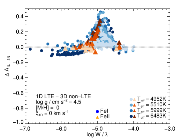
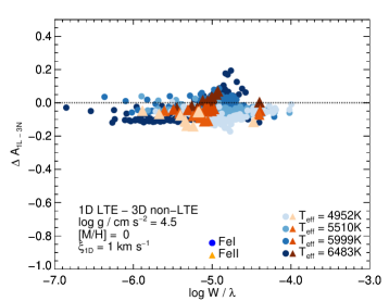
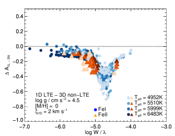
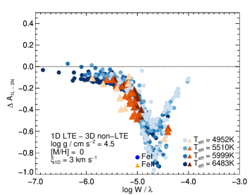
Figure 3: $\Delta A_{\text{1L-3N}}$ against $\log W/\lambda{}$, for different lines of ${Fe\textsc{I}}$ and ${Fe\textsc{II}}$ (symbols), and different values of $\xi_{\text{mic;1D}}$ (panels). Lighter colours represent smaller $T_{\mathrm{eff}}$. The results are shown for $\log{g}=4.5$ and $\mathrm{\left[M/H\right]}=0$.

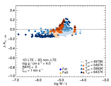
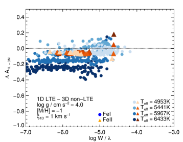
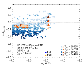
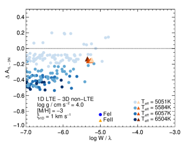
Figure 4: $\Delta A_{\text{1L-3N}}$ against $\log W/\lambda{}$, for different lines of ${Fe\textsc{I}}$ and ${Fe\textsc{II}}$ (symbols), and different values of $\mathrm{\left[M/H\right]}$ (panels). Lighter colours represent smaller $T_{\mathrm{eff}}$. The results are shown for $\log{g}=4.0$ and $\xi_{\text{mic;1D}}=1$.

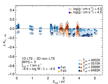
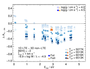
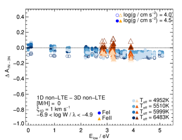
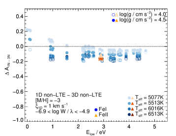
Figure 5: $\Delta A_{\text{1L-3N}}$ (upper panels) and $\Delta A_{\text{1N-3N}}$ (lower panels) against $E_{\text{low}}{}$, for different lines of ${Fe\textsc{I}}$ and ${Fe\textsc{II}}$ (symbols), and different values of $\mathrm{\left[M/H\right]}$ (columns). Lighter colours represent smaller $T_{\mathrm{eff}}$. The results are shown for $\xi_{\text{mic;1D}}=1\,\mathrm{km\,s^{-1}}$ and $-6.9<\log W/\lambda<-4.9$.

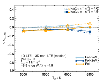
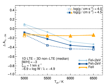
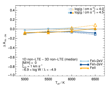
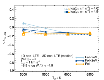
Figure 6: $\Delta A_{\text{1L-3N}}$ (upper panels) and $\Delta A_{\text{1N-3N}}$ (lower panels) against $T_{\mathrm{eff}}{}$, averaged over lines of ${Fe\textsc{I}}$ with $E_{\text{low}}<2\,\mathrm{eV}$ and $E_{\text{low}}>2\,\mathrm{eV}$ as well as over lines of ${Fe\textsc{II}}$, for different values of $\mathrm{\left[M/H\right]}$ (columns). The results are shown for $\xi_{\text{mic;1D}}=1\,\mathrm{km\,s^{-1}}$ and $-6.9<\log W/\lambda<-4.9$.

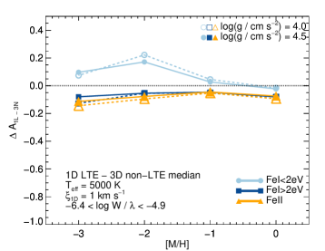
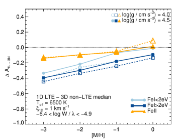
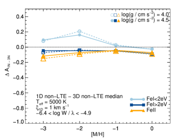
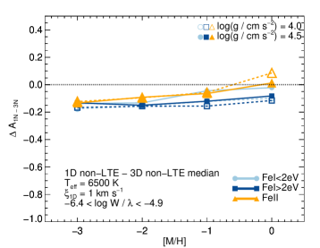
Figure 7: $\Delta A_{\text{1L-3N}}$ (upper panels) and $\Delta A_{\text{1N-3N}}$ (lower panels) against $\mathrm{\left[M/H\right]}$, averaged over lines of ${Fe\textsc{I}}$ with $E_{\text{low}}<2\,\mathrm{eV}$ and $E_{\text{low}}>2\,\mathrm{eV}$ as well as over lines of ${Fe\textsc{II}}$, for different values of $T_{\mathrm{eff}}{}$ (columns). The results are shown for $\xi_{\text{mic;1D}}=1\,\mathrm{km\,s^{-1}}$ and $-6.9<\log W/\lambda<-4.9$.

3.1 Partially saturated lines

Fig. 3 illustrates the behaviour of $\Delta A_{\text{1L-3N}}$ with $\log W/\lambda$ for $\log{g}=4.5$ and $\mathrm{\left[M/H\right]}=0$, and $\xi_{\text{mic;1D}}$ between $0\,\mathrm{km\,s^{-1}}$ and $3\,\mathrm{km\,s^{-1}}$. Depending on $\xi_{\text{mic;1D}}$, the plots either have a peak or a trough at $\log W/\lambda\approx-4.8$: for small $\xi_{\text{mic;1D}}$, $\Delta A_{\text{1L-3N}}$ reaches up to $+0.4\,\mathrm{dex}$, while for large $\xi_{\text{mic;1D}}$, $\Delta A_{\text{1L-3N}}$ reaches down to $-1.0\,\mathrm{dex}$. Fig. 4 illustrates this same behaviour for $\log{g}=4.0$, $\xi_{\text{mic;1D}}=1\,\mathrm{km\,s^{-1}}$, and different values of $\mathrm{\left[M/H\right]}$. The peak position is roughly the same in these plots; it becomes less apparent towards smaller $\mathrm{\left[M/H\right]}$ as the studied lines become weaker.

The peaked appearance of $\Delta A_{\text{1L-3N}}$ is typical of abundance differences. For example, it can be seen for Na I in Fig. 5 of Lind et al. (2011), for K I in Fig. 13 of Reggiani et al. (2019), and for C I and O I in Fig. 7 of Amarsi et al. (2019b). It is related to lines leaving the linear part of the curve of growth and becoming partially saturated as $\log W/\lambda$ increases. When this happens first in 1D LTE, a large increase in $A\left({\mathrm{Fe}}\right)_{\text{1L}}$ is needed to match $A\left({\mathrm{Fe}}\right)_{\text{3N}}$. This results in large, positive values of $\Delta A_{\text{1L-3N}}$. Vice versa, when partial saturation first occurs in the 3D non-LTE model, one finds large, negative values of $\Delta A_{\text{1L-3N}}$. At even larger $\log W/\lambda\gtrsim-4.8$, both 1D LTE and 3D non-LTE lines are partially saturated, and the behaviour of the abundance differences again reflect those in the weak-line regime. Further discussion of this effect may be found in Sect. 3.1 of Lind et al. (2011) and Sect. 3.2.3 of Amarsi et al. (2019b).

The main effect of $\xi_{\text{mic;1D}}$ in Fig. 3 can be understood in terms of the behaviour of $\Delta A_{\text{1L-3N}}$ with $\log W/\lambda$. Adopting a smaller $\xi_{\text{mic;1D}}$ would mean that the 1D LTE lines become partially saturated and leave the linear part of the curve of growth before the 3D non-LTE lines (first panel of Fig. 3). Conversely, adopting a larger $\xi_{\text{mic;1D}}$ desaturates the 1D LTE lines; they leave the linear part of the curve of growth and become partially saturated after the 3D non-LTE lines (lower two panels of Fig. 3). The effect of $\xi_{\text{mic;1D}}$ is smaller for lines with $\log W/\lambda\ll-4.8$ and $\log W/\lambda\gg-4.8$. In the former case (the weak-line regime), the line core is not yet saturated and so does not suffer so strongly from $\xi_{\text{mic;1D}}$; while in the latter case (strong lines), the equivalent widths are dominated by the area spanned by extended pressure broadened wings.

The effects described above are 3D effects. As such, $\Delta A_{\text{1N-3N}}$ displays a qualitatively similar behaviour to $\Delta A_{\text{1L-3N}}$. The behaviour is also qualitatively similar for other values of $\log{g}$ and $\mathrm{\left[M/H\right]}$ not shown in the figures.

For clarity and brevity, the remaining parts of Sect. 3 are based on lines with $-6.9<\log W/\lambda<-4.9$, and the choice of $\xi_{\text{mic;1D}}=1\,\mathrm{km\,s^{-1}}$. For this choice of $\xi_{\text{mic;1D}}$, Fig. 3 indicates that the 1D LTE and 3D non-LTE model lines leave the linear part of the curve of growth at roughly the same point. By adopting this $\xi_{\text{mic;1D}}$, and only considering weak lines, the discussion and interpretation of the abundance differences is greatly simplified.

3.2 Weak Fe I lines

At $\mathrm{\left[M/H\right]}=0$, for $\xi_{\text{mic;1D}}=1\,\mathrm{km\,s^{-1}}$, the upper left panels of Fig. 5 show that for weak Fe I lines, $\Delta A_{\text{1L-3N}}$ ranges from $-0.15\,\mathrm{dex}$ to $+0.10\,\mathrm{dex}$. At $\mathrm{\left[M/H\right]}=-3$, the right panels show that $\Delta A_{\text{1L-3N}}$ reaches $-0.5$ at high $T_{\mathrm{eff}}$ and low $\log{g}$, and $+0.2\,\mathrm{dex}$ at low $T_{\mathrm{eff}}$, at least for the selection of Fe I lines considered here. The overall range of results is similar for $\Delta A_{\text{1N-3N}}$ at $\mathrm{\left[M/H\right]}=0$; although, interestingly, the scatter in the plots is smaller than for $\Delta A_{\text{1L-3N}}$. At low $\mathrm{\left[M/H\right]}$, however, the lines with the most negative values of $\Delta A_{\text{1L-3N}}$ show less severe values of $\Delta A_{\text{1N-3N}}$, which only reaches down to $-0.2\,\mathrm{dex}$ at $\mathrm{\left[M/H\right]}=-3$.

These abundance differences are due to the combination of 3D and non-LTE effects that are rather complicated to disentangle (Sect. 3.2 and 3.3 of Amarsi et al. 2016). The 3D effects can be due to differences in the mean model stellar atmosphere stratifications, the presence of inhomogeneities, and horizontal radiative transfer. These various phenomena are complicated, with the 3D models being either shallower or steeper on average than the 1D models depending on the stellar parameters (Bergemann et al., 2012), and with the sign of $\Delta A_{\text{1N-3N}}$ and $\Delta A_{\text{1L-3N}}$ varying across the granulation pattern and line formation height (Holzreuter & Solanki, 2013). They also depend on the particular choice of $\xi_{\text{mic;1D}}$, with larger values shifting $\Delta A_{\text{1L-3N}}$ and $\Delta A_{\text{1N-3N}}$ downwards. The non-LTE effects on Fe I, on the other hand, can be due to the over-ionisation of the minority species that would act to increase the inferred $A\left({\mathrm{Fe}}\right)$, or photon losses in the line cores that act to reduce it, broadly speaking (Kostik et al., 1996). This competition can be seen in the comparison of the 3D LTE and 3D non-LTE profiles in the upper right panel of Fig. 2, where the 3D non-LTE profile is narrower due to over-ionisation, but has a similar core flux depression due to photon losses.

The 3D and non-LTE effects may couple to each other in complex ways. Nevertheless, the overall trend is that $\Delta A_{\text{1L-3N}}$ and $\Delta A_{\text{1N-3N}}$ are usually the most negative for the high $T_{\mathrm{eff}}$, low $\log{g}$, and, at least for higher $T_{\mathrm{eff}}$, low $\mathrm{\left[M/H\right]}$ models (as expected from previous studies; Sect. 1). These trends are more clearly visible in Fig. 6 and Fig. 7, which show the median results for Fe I lines of low and high excitation potential. The left panels of Fig. 7 show that there are peaks in $\Delta A_{\text{1L-3N}}$ and $\Delta A_{\text{1N-3N}}$ at $\mathrm{\left[M/H\right]}=-2$ and $T_{\mathrm{eff}}=5000\,\mathrm{K}$, for Fe I lines of low excitation potential. This reflects the competition between (reverse) granulation effects (driving weaker lines in 3D corresponding to more positive $\Delta A_{\text{1L-3N}}$ and $\Delta A_{\text{1N-3N}}$) and the effect of the lower temperatures in the upper layers of the 3D models (driving stronger lines in 3D corresponding to more negative $\Delta A_{\text{1L-3N}}$ and $\Delta A_{\text{1N-3N}}$), with the latter effect becoming much more pronounced at $\mathrm{\left[M/H\right]}=-3$.

Over-ionisation is certainly larger for such stars, because the escaping UV flux increases for such stars, and also because more compact stars have more efficient collisional rates that help counteract these effects (Lind et al., 2012). At smaller $\mathrm{\left[M/H\right]}$, photon losses are also typically weaker due to the smaller strengths of the Fe I lines. The 3D effects might in general also be expected to be more severe for such stars, with larger granulation contrasts and thus larger fluctuations in the atmosphere (Magic et al., 2013). In general, as noted above, this does not immediately imply more negative values of $\Delta A_{\text{1N-3N}}$ and $\Delta A_{\text{1L-3N}}$; although, at low $\mathrm{\left[M/H\right]}$ the steeper mean stratifications of the 3D models act to enhance the non-LTE over-ionisation (Nordlander et al., 2017).

Fig. 5 indicates that the abundance differences for weak Fe I lines depend on $E_{\text{low}}$. For the cooler models, $\Delta A_{\text{1L-3N}}$ and $\Delta A_{\text{1N-3N}}$ even change sign with increasing $E_{\text{low}}$. At $\mathrm{\left[M/H\right]}=0$ there is a roughly linear trend such that $\Delta A_{\text{1L-3N}}$ and $\Delta A_{\text{1N-3N}}$ decrease by around $-0.05\,\mathrm{dex}$ to $-0.1\,\mathrm{dex}$ as $E_{\text{low}}$ increases from $0\,\mathrm{eV}$ to $5\,\mathrm{eV}$, which reflects a combination of differences in the mean stratifications and inhomogeneities at different depths. At $\mathrm{\left[M/H\right]}=-3$ the relationship becomes more complicated, with an upturn at $E_{\text{low}}\approx 3\,\mathrm{eV}$. This value corresponds to the broad peak in ionisation and recombination events in Fig. 3 of Lind et al. (2012); these levels are the ones most likely to absorb hot UV photons and undergo over-ionisation directly.

These trends with $E_{\text{low}}$ imply that 3D non-LTE effects are implicit in 1D LTE spectroscopic determinations of $T_{\mathrm{eff}}$ that are based on the excitation balance of Fe I lines. It is beyond the scope of the present study to attempt to derive grids of $T_{\mathrm{eff}}$ corrections here. Such an effort would be complicated by the non-linear behaviour of $\Delta A_{\text{1L-3N}}$ with $E_{\text{low}}$ and the strong dependence on $\log W/\lambda$ (Sect. 3.1), such that the extent of the $T_{\mathrm{eff}}$ errors would depend on the particular set of Fe I lines under consideration.

3.3 Weak Fe II lines

At $\mathrm{\left[M/H\right]}=0$, for $\xi_{\text{mic;1D}}=1\,\mathrm{km\,s^{-1}}$, the left panels of Fig. 5 show that for weak Fe II lines, $\Delta A_{\text{1L-3N}}$ ranges from $-0.15\,\mathrm{dex}$ to $+0.10\,\mathrm{dex}$, similar to Fe I (Sect. 3.2). There is a trend of more positive values towards larger $T_{\mathrm{eff}}$ and smaller $\log{g}$, as can also be seen in the upper left panel of Fig. 6. At $\mathrm{\left[M/H\right]}=-3$, unfortunately there is just one Fe II line in the current study with $-6.9<\log W/\lambda<-4.9$. For this line the value of $\Delta A_{\text{1L-3N}}$ is between $-0.11\,\mathrm{dex}$ and $-0.15\,\mathrm{dex}$, changing mildly with $T_{\mathrm{eff}}$ or $\log{g}$; it gives rise to flat trends in the right panels of Fig. 6. The non-LTE effects in Fe II lines are not significant at $\mathrm{\left[M/H\right]}=0$, and so $\Delta A_{\text{1N-3N}}\approx\Delta A_{\text{1L-3N}}$. These abundance differences are thus primarily driven by 3D LTE effects, which are discussed in Amarsi et al. (2019b).

There are, however, non-LTE effects for the warmest stars at the lowest $\mathrm{\left[M/H\right]}$. This can be seen via the subtle differences between the upper and lower right panels of Fig. 5, which indicate small 1D non-LTE effects. We note that Fe II lines can suffer from over-excitation and become weaker relative to 1D LTE (translating to larger inferred $A\left({\mathrm{Fe}}\right)$ in non-LTE). The non-LTE effects on Fe II lines are even larger in the metal-poor 3D models due to their steeper gradients (Shchukina et al., 2005). The 3D LTE versus 3D non-LTE abundance differences can be estimated by using the logarithmic ratios of equivalent widths. They are the most negative for the high $T_{\mathrm{eff}}$, low $\log{g}$, and low $\mathrm{\left[M/H\right]}$ models (for similar reasons given in Sect. 3.2). At $T_{\mathrm{eff}}\approx 6500\,\mathrm{K}$, $\log{g}=4.0$, and $\mathrm{\left[M/H\right]}=-3$, these differences are $-0.09\pm 0.05\,\mathrm{dex}$, averaging over all the Fe II lines. The differences are already much less severe for the model with similar $T_{\mathrm{eff}}$ and $\log{g}$ but with $\mathrm{\left[M/H\right]}=-2\,\mathrm{dex}$, where they amount to $-0.02\pm 0.01$.

Fig. 5 illustrates that for the cooler models, $\Delta A_{\text{1L-3N}}$ typically has the same sign for Fe II lines as for Fe I lines of $2\lesssim E_{\text{low}}/\mathrm{eV}\lesssim 5$; usually they are both negative. The consequence of this is that 1D LTE analyses of lines of either of these species may underestimate $A\left({\mathrm{Fe}}\right)$. On the other hand, the fact that the abundance differences for Fe I and Fe II usually have the same sign helps to counteract the systematic errors on 1D LTE spectroscopic determinations of $\log{g}$ to some extent, at least for $T_{\mathrm{eff}}\lesssim 6000\,\mathrm{K}$.

4 Interpolation in stellar and line parameters

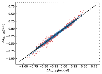
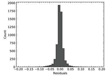
Figure 8: Predicted versus actual $\Delta A_{\text{1L-3N}}$ colour-coded by the size of the interpolation error (upper panel), and distribution of interpolation errors in $\mathrm{dex}$ (lower panel) for the routine presented in Sect. 4. Interpolation was carried out over stellar and line parameters simultaneously.

The derived values of $\Delta A_{\text{1L-3N}}$ illustrated above (Sect. 3) were used to analyse standard stars, the results of which are presented in the following section (Sect. 5). To do so, it was necessary to interpolate these abundance differences as a function of stellar parameters ($T_{\mathrm{eff}}$, $\log{g}$, $A\left({\mathrm{Fe}}\right)_{\text{3N}}$, and $\xi_{\text{mic;1D}}$) and line parameters ($E_{\text{low}}$, $E_{\text{up}}$, and $\log{gf}$).

Several different approaches based on simple linear and spline interpolation and more sophisticated machine-learning algorithms were explored. Ultimately, following Wang et al. (2021), the interpolation model was based on multi-layer perceptrons (MLP), which is a feed-forward fully connected neural network that connects the input and output layers through $n_{l}$ number of hidden layers. The hidden layers contain $n$ neurons, and each neuron is connected to all the neurons in the previous layers with weights fitted through back-propagation training. The models are constructed using the MLPRegressor class from the scikit-learn python library (Pedregosa et al., 2012).

Three different MLP models were built, separating the data into three groups: Fe I lines with $E_{\text{low}}<2\,\mathrm{eV}$; Fe I lines with $E_{\text{low}}>2\,\mathrm{eV}$; and Fe II lines. This was found to give more reliable results than building a single MLP model for these three groups. The tolerance was set to $10^{-5}$, and the activation function used was the Rectified Linear Unit function (ReLU). Via a $5$-fold cross-validation scheme, the network size was set to $n_{l}=3$ and $n=200$, and the L2 regularisation term (that prevents overfitting) was set to $\alpha=5\times 10^{-4}$, $7\times 10^{-4}$, and $10^{-2}$ for the three different MLP models, respectively. Via a $k$-fold cross-validation scheme using the MLP models, a select number of severe outliers, reflecting the difficulties in determining equivalent widths (Sect. 2.4), were identified; the MLP models were then rebuilt, with these data removed.

To evaluate the performance of the MLP models, the datasets were randomly divided into a training set ($80\%$ of the data) and a test set ($20\%$ of the data). The three MLP models were trained on their respective training sets, and then applied to their respective test sets. The overall performance of the interpolation routine is illustrated in Fig. 8, where the histogram shows that the residuals of the three MLP models have standard deviations of $0.024$, $0.017$, and $0.016\,\mathrm{dex}$, respectively. They reflect the expected $1\,\sigma$ interpolation error when looking at one Fe I or Fe II line in one star. These interpolation errors translate to scatter in plots of line-by-line $A\left({\mathrm{Fe}}\right)$ and average out when using sufficiently large numbers of Fe I and Fe II lines. Moreover the scatter plot in Fig. 8 shows that the largest interpolation errors tend to occur where $\Delta A_{\text{1L-3N}}$ is larger.

The input parameters of the interpolation routine are the stellar parameters and line parameters listed above: $T_{\mathrm{eff}}$, $\log{g}$, $A\left({\mathrm{Fe}}\right)_{\text{3N}}$, and $\xi_{\text{mic;1D}}$ as well as $E_{\text{low}}$, $E_{\text{up}}$, and $\log{gf}$. The interpolation routine also returns results for stars outside of the grid of stellar parameters ($T_{\mathrm{eff}}$ between $5000\,\mathrm{K}$ and $6500\,\mathrm{K}$, $\log{g}$ between $4.0\,\mathrm{dex}$ and $4.5\,\mathrm{dex}$, and $A\left({\mathrm{Fe}}\right)_{\text{3N}}$ between $4.5\,\mathrm{dex}$ and $7.5\,\mathrm{dex}$) and line parameters (see Fig. 1 and Sect. 2.4). In such cases the returned results are intrinsically more uncertain, and should be treated with caution. The possible impact of interpolation and extrapolation in line parameters is discussed more in Sect. 5.4 in the context of the application to standard stars.

The input parameter $A\left({\mathrm{Fe}}\right)_{\text{3N}}$ is the 3D non-LTE iron abundance. Since this is usually unknown, in principle this routine needs to be applied iteratively. In practice, when the abundance differences are small or do not strongly vary with $\mathrm{\left[M/H\right]}$, it is safe to make the approximation $A\left({\mathrm{Fe}}\right)_{\text{3N}}\approx A\left({\mathrm{Fe}}\right)_{\text{1L}}$, thus avoiding any iterations and allowing for a quick estimate of the abundance correction (which is given by the negative of $\Delta A_{\text{1L-3N}}$). When the abundance differences are larger, there can be a notable difference in the final result. For example, in the analysis of the star HD 84937 (Sect. 5), the results for individual Fe I lines changed by up to $0.05\,\mathrm{dex}$ when iterations were neglected, and the mean difference changed by $0.016\,\mathrm{dex}$. These differences are, however, within the overall uncertainty in $A\left({\mathrm{Fe}}\right)$ for this star. Nevertheless, in the present work, the routine was always applied iteratively to avoid these small systematic errors.

To compare between 1D non-LTE and 3D non-LTE $A\left({\mathrm{Fe}}\right)$, an analogous interpolation routine was constructed to correct for 1D non-LTE effects. To facilitate a fair comparison, this was based on the calculations from the $32$ ATMO models, rather than the finer grid of MARCS models (Sect. 2.1). This 1D non-LTE interpolation routine uses the same input parameters as the 3D non-LTE one discussed above. When applying this interpolation routine, it was assumed that the 1D LTE and 1D non-LTE values of $\xi_{\text{mic;1D}}{}$ were identical. In practice, calibrations of $\xi_{\text{mic;1D}}{}$ based on flattening trends with a (reduced) equivalent width can be sensitive to non-LTE effects up to the order of $10\%$ (Amarsi et al., 2016).

5 Application to standard stars

Table 2: Adopted values and uncertainties for $T_{\mathrm{eff}}$, $\log{g}$, and (for the 1D models) $\xi_{\text{mic;1D}}$, as well as 1D non-LTE $\mathrm{\left[Fe/H\right]}$ from the literature. Final columns show the values of [Fe/H] derived in this study in 1D LTE, 1D non-LTE, and 3D non-LTE (mean of $\mathrm{\left[Fe/H\right]}_{{Fe\textsc{I}}}$ and $\mathrm{\left[Fe/H\right]}_{{Fe\textsc{II}}}$ values weighted by statistical and stellar parameter uncertainties).

Name	$T_{\mathrm{eff}}/\mathrm{K}$	$\log{g/\mathrm{cm\,s^{-2}}}$	$\xi_{\text{mic;1D}}/\mathrm{km\,s^{-1}}$	$\mathrm{\left[Fe/H\right]}_{\text{Lit.}}$	Ref.	$\mathrm{\left[Fe/H\right]}_{\text{1L}}$	$\mathrm{\left[Fe/H\right]}_{\text{1N}}$	$\mathrm{\left[Fe/H\right]}_{\text{3N}}$
Sun	$5772$	$4.44$	$1.00$	$0.00$	a	$0.00$	$0.00$	$0.00$
Procyon	$6554\pm 84$	$4.00\pm 0.02$	$1.66\pm 0.11$	$-0.02\pm 0.08$	b	$0.04\pm 0.03$	$0.05\pm 0.03$	$0.11\pm 0.03$
HD 84937	$6356\pm 97$	$4.13\pm 0.03$	$1.39\pm 0.24$	$-2.06\pm 0.08$	b,c	$-2.04\pm 0.03$	$-2.03\pm 0.03$	$-1.96\pm 0.03$
HD 140283	$5792\pm 55$	$3.65\pm 0.02$	$1.56\pm 0.20$	$-2.29\pm 0.11$	b,d	$-2.42\pm 0.03$	$-2.38\pm 0.03$	$-2.28\pm 0.02$

Table 3: Breakdown of uncertainties propagated onto $A\left({\mathrm{Fe}}\right)$. The uncertainties in solar parameters are neglected.

Name	1D LTE				1D non-LTE				3D non-LTE
	$\sigma_{\text{stat.}}$	$\sigma_{T_{\mathrm{eff}}}$	$\sigma_{\log{g}}$	$\sigma_{\xi_{\text{mic;1D}}}$	$\sigma_{\text{stat.}}$	$\sigma_{T_{\mathrm{eff}}}$	$\sigma_{\log{g}}$	$\sigma_{\xi_{\text{mic;1D}}}$	$\sigma_{\text{stat.}}$	$\sigma_{T_{\mathrm{eff}}}$	$\sigma_{\log{g}}$	$\sigma_{\xi_{\text{mic;1D}}}$
	Fe I				Fe I
Sun	$0.011$	$0.000$	$0.000$	$0.000$	$0.010$	$0.000$	$0.000$	$0.000$	$0.011$	$0.000$	$0.000$	$0.000$
Procyon	$0.005$	$0.050$	$0.000$	$0.013$	$0.006$	$0.055$	$0.001$	$0.011$	$0.006$	$0.064$	$0.003$	$0.001$
HD 84937	$0.008$	$0.068$	$0.000$	$0.015$	$0.005$	$0.065$	$0.003$	$0.011$	$0.007$	$0.074$	$0.003$	$0.002$
HD 140283	$0.010$	$0.045$	$0.000$	$0.018$	$0.007$	$0.049$	$0.002$	$0.014$	$0.008$	$0.053$	$0.003$	$0.002$
	Fe II				Fe II
Sun	$0.016$	$0.000$	$0.000$	$0.000$	$0.017$	$0.000$	$0.000$	$0.000$	$0.018$	$0.000$	$0.000$	$0.000$
Procyon	$0.024$	$0.005$	$0.008$	$0.024$	$0.024$	$0.005$	$0.008$	$0.024$	$0.023$	$0.001$	$0.009$	$0.003$
HD 84937	$0.014$	$0.014$	$0.011$	$0.011$	$0.013$	$0.012$	$0.011$	$0.012$	$0.014$	$0.010$	$0.010$	$0.000$
HD 140283	$0.020$	$0.008$	$0.008$	$0.017$	$0.021$	$0.008$	$0.010$	$0.016$	$0.017$	$0.007$	$0.007$	$0.007$

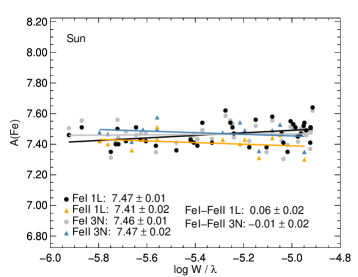
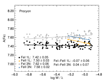
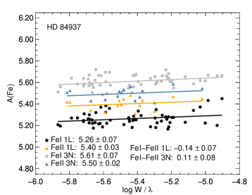
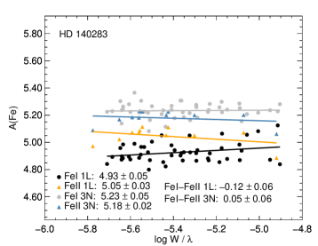
Figure 9: Line-by-line $A\left({\mathrm{Fe}}\right)$ versus $\log W/\lambda$. We note that 1D LTE and 3D non-LTE Fe I and Fe II lines are indicated separately, with least-squares fits being overdrawn.

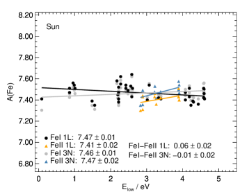
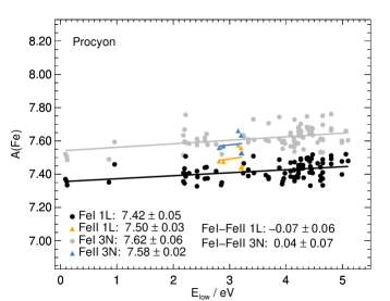
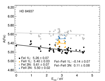
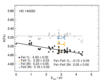
Figure 10: Line-by-line $A\left({\mathrm{Fe}}\right)$ versus $E_{\text{low}}$. We note that 1D LTE and 3D non-LTE Fe I and Fe II lines are indicated separately, with least-squares fits being overdrawn.

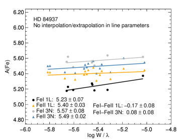
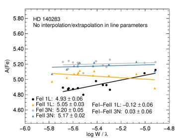
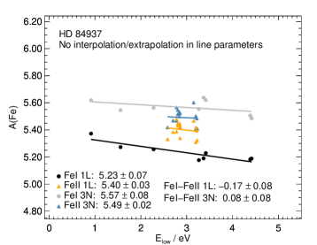
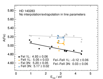
Figure 11: Same as Fig. 9 and Fig. 10, but for the metal-poor stars and restricted to the Fe I lines that are included within the $\Delta A_{\text{1L-3N}}$ grid (Fig. 1), and using the extended 3D LTE grid from Amarsi et al. (2019b) for Fe II lines.

Table 4: $A\left({\mathrm{Fe}}\right)$ inferred from Fe I and Fe II lines in 1D LTE, 1D non-LTE, and 3D non-LTE. Errors reflect statistical and stellar parameter uncertainties (not model uncertainties).

Name	1D LTE		1D non-LTE		3D non-LTE
	Fe I	Fe II	Fe I	Fe II	Fe I	Fe II
Sun	$7.47\pm 0.01$	$7.41\pm 0.02$	$7.45\pm 0.01$	$7.41\pm 0.02$	$7.46\pm 0.01$	$7.47\pm 0.02$
Procyon	$7.42\pm 0.05$	$7.50\pm 0.03$	$7.45\pm 0.06$	$7.49\pm 0.03$	$7.62\pm 0.06$	$7.58\pm 0.02$
HD 84937	$5.26\pm 0.07$	$5.40\pm 0.03$	$5.43\pm 0.07$	$5.38\pm 0.02$	$5.61\pm 0.07$	$5.50\pm 0.02$
HD 140283	$4.93\pm 0.05$	$5.05\pm 0.03$	$5.08\pm 0.05$	$5.03\pm 0.03$	$5.23\pm 0.05$	$5.18\pm 0.02$

Table 5: Ionisation imbalance $\mathrm{A\left({\mathrm{Fe}}\right)_{{Fe\textsc{I}}}-A\left({\mathrm{Fe}}\right)_{{Fe\textsc{II}}}}$ in 1D LTE, 1D non-LTE, and 3D non-LTE. Errors reflect statistical and stellar parameter uncertainties (not model uncertainties).

Name	1D LTE	1D non-LTE	3D non-LTE
Sun	$0.06\pm 0.02$	$0.04\pm 0.02$	$-0.01\pm 0.02$
Procyon	$-0.07\pm 0.06$	$-0.04\pm 0.07$	$0.04\pm 0.07$
HD 84937	$-0.14\pm 0.07$	$0.05\pm 0.07$	$0.11\pm 0.08$
HD 140283	$-0.12\pm 0.06$	$0.05\pm 0.06$	$0.05\pm 0.06$

5.1 Stellar parameters

This section demonstrates the possible impact of $\Delta A_{\text{1L-3N}}$ in practice. For this purpose, as well as the Sun, the standard stars Procyon (HD 61421), HD 84937, and HD 140283 were selected to be analysed. These stars are interesting in this context because they are located close to different edges of the grid of $\Delta A_{\text{1L-3N}}$ in $T_{\mathrm{eff}}$ and $\mathrm{\left[M/H\right]}$. Moreover, they are all in the original GBS catalogue (Heiter et al., 2015), implying that they have relatively well-constrained stellar parameters, and that they are of astrophysical importance for calibrating and validating spectroscopic studies (Pancino et al., 2017; Buder et al., 2021). Lastly, the Sun (Asplund et al., 2021) and the two metal-poor stars (Amarsi et al., 2016) have previously been studied using the same or similar model atoms, and thus serve as a rough consistency check of the grid-based approach adopted here.

The adopted stellar parameters of these stars are given in Table 2. Where possible, the parameters were updated to account for the most recent and reliable measurements. These stars were analysed in slightly different ways, as discussed below (Sect. 5.2).

5.2 Analysis

The Sun was analysed in the simplest way. Line-by-line 1D LTE $A\left({\mathrm{Fe}}\right)$ values measured in the solar flux atlas of Kurucz et al. (1984) were taken from Allende Prieto et al. (2002). The analysis was restricted to weak lines with $\log W/\lambda<-4.9$ because partially saturated lines are more sensitive to uncertainties in the equivalent widths and also correspond to larger values of $\Delta A_{\text{1L-3N}}$ (Sect. 3.1). The $A\left({\mathrm{Fe}}\right)$ values for the Fe II lines were corrected for the more precise values of $\log{gf}$ provided in Meléndez & Barbuy (2009). The 1D LTE values were then corrected to obtain 3D non-LTE values, using the interpolation routine described in Sect. 4. The interpolation routine uses the 3D non-LTE $A\left({\mathrm{Fe}}\right)$ as an input parameter, and returns the 1D LTE versus 3D non-LTE abundance difference. Since the 3D non-LTE $A\left({\mathrm{Fe}}\right)$ is initially unknown, the interpolation routine was applied iteratively, using the 1D LTE value as the first guess.

For Procyon (HD 61421), Allende Prieto et al. (2002) also provide 1D LTE $A\left({\mathrm{Fe}}\right)$. However, their $T_{\mathrm{eff}}$ and $\log{g}$ are smaller than those recommended by Chiavassa et al. (2012) and Heiter et al. (2015). Moreover, their Fe II line list mostly consists of partially saturated lines; combined with their choice of $\xi_{\text{mic;1D}}=2.2\,\mathrm{km\,s^{-1}}$, the corresponding $\Delta A_{\text{1L-3N}}$ becomes large (Sect. 3.1) and more sensitive to the way in which the 1D LTE abundances were derived. Instead, this star was analysed using the lines in Tables 4 and 5 of Jofré et al. (2014) (the same line list that is the basis of this study, and is illustrated in Fig. 1). The authors provide up to five different measurements of the equivalent width for each line (labelled epinarbo, ucm, porto, bologna, and ulb). For a given line, 1D LTE values of $A\left({\mathrm{Fe}}\right)$ were determined based on each of these measurements separately via spline interpolation of the theoretical grid of equivalent widths based on MARCS model stellar atmospheres (Sect. 2). The results from the (at most) five different equivalent widths were then individually compared to the overall mean 1D LTE value from all of the Fe I lines. Those that were more than $2\,\sigma$ from the mean were removed, where $\sigma$ here is the standard deviation of $A\left({\mathrm{Fe}}\right)$ from the different Fe I lines. This sigma clipping was evaluated using the 1D LTE results; the exact same clipping was then later adopted for the 3D non-LTE analysis. The surviving data were then averaged together to get a final 1D LTE $A\left({\mathrm{Fe}}\right)$ for that particular star and from that particular Fe I line. This proceeded iteratively. An identical approach was adopted for Fe II lines, except comparing them with the overall mean 1D LTE $A\left({\mathrm{Fe}}\right)$ from Fe II lines. Lastly, the 1D LTE values of $A\left({\mathrm{Fe}}\right)$ were corrected to obtain 3D non-LTE values, using the interpolation routine described in Sect. 4 in the same way as was done for the Sun, albeit with $0$th-order extrapolation in $T_{\mathrm{eff}}$ and $A\left({\mathrm{Fe}}\right)_{\text{3N}}$ (adopting the values at $T_{\mathrm{eff}}=6500\,\mathrm{K}$ and $A\left({\mathrm{Fe}}\right)_{\text{3N}}=7.5$). As for the Sun, this analysis was restricted to weak lines with $\log W/\lambda<-4.9$.

The analyses of the metal-poor stars HD 84937 and HD 140283 that were presented in Jofré et al. (2014) are based on a few lines, especially for Fe II. Here, these stars are instead analysed using the lines, equivalent widths, and theoretical 1D LTE grids presented in Amarsi et al. (2016). The stellar parameters were updated to those given in Table 2. In all other ways, the analysis proceeded as described for Procyon. In particular, the interpolation routine provided in this work was iteratively used to correct the 1D LTE to 3D non-LTE values as before, with $0$th-order extrapolation in $\log{g}$ for HD 140283 (adopting the value at $\log{g}=4.0$).

Statistical uncertainties were calculated for each star as the standard error in the mean for Fe I and Fe II separately. These primarily reflect uncertainties in the equivalent width measurements and adopted values of $\log{gf}$. For Procyon, HD 84937, and HD 140283, systematic uncertainties were estimated by repeating the above steps (though for the purposes of this study with a fixed selection of lines and equivalent widths in the case of Procyon), while perturbing $T_{\mathrm{eff}}$, $\log{g}$, and $\xi_{\text{mic;1D}}$ individually by the uncertainties listed in Table 2. Systematic uncertainties were neglected for the Sun. The final uncertainties were obtained by adding these difference sources of uncertainty together in quadrature. These uncertainties are presented in Table 3. As seen therein, the sensitivity to $\xi_{\text{mic;1D}}$ reaches almost to zero for the 3D non-LTE runs for the Sun and HD 84937 because these models do not adopt any extra broadening parameters; for Procyon and HD 140283, the uncertainty is slightly non-zero because of the $0$th-order extrapolation in stellar parameters.

The 1D non-LTE analysis proceeded in almost the same way as the 3D non-LTE one. The only difference was that the 1D non-LTE interpolation routine was used instead of the 3D non-LTE one, as discussed in Sect. 4.

5.3 Results

The results for $A\left({\mathrm{Fe}}\right)$ are illustrated in Fig. 9 and Fig. 10. Estimates of $\mathrm{\left[Fe/H\right]}$ from the 1D LTE, 1D non-LTE, and 3D non-LTE models are given in Table 2. These are based on the weighted means of $\mathrm{\left[Fe/H\right]}_{\text{{Fe {I}}}}$ and $\mathrm{\left[Fe/H\right]}_{\text{{Fe {II}}}}$, with the uncertainties summarised Table 3, and adopting the 1D LTE, 1D non-LTE, and 3D non-LTE solar values (respectively) separately for the $A\left({\mathrm{Fe}}\right)_{\text{{Fe {I}}}}$ and $A\left({\mathrm{Fe}}\right)_{\text{{Fe {II}}}}$ derived here and given in Table 4. In practice, the Fe II lines are given a much higher weight than the Fe I lines in these weighted means because of the high sensitivity of the Fe I lines to $T_{\mathrm{eff}}$ (Table 3).

We make some general remarks here, before discussing each star individually in Sections 5.3.1—5.3.4. There are significant 3D non-LTE effects on ${Fe\textsc{I}}$ or ${Fe\textsc{II}}$, or both, for all four stars. After averaging over lines, the 3D non-LTE effects act to increase $A\left({\mathrm{Fe}}\right)$ and correspond to negative values of $\Delta A_{\text{1L-3N}}$ overall, as is generally expected of Fe I lines with $E_{\text{low}}>2\,\mathrm{eV}$ and of Fe II lines (Sect. 3.3). For Fe I, the largest difference is for HD 84937 ($0.35\,\mathrm{dex}$), while for Fe II the largest difference is for HD 140283 ($0.15\,\mathrm{dex}$).

Comparing the 1D LTE, 1D non-LTE, and 3D non-LTE results helps disentangle the 3D effects and the non-LTE effects, to some extent. For Fe II, the line-averaged 1D non-LTE results agree with the 1D LTE ones to $0.02\,\mathrm{dex}$ (Table 4); these lines are primarily susceptible to 3D effects (Sect. 3.3). There is more variation for Fe I. For the Sun and Procyon (HD 61421), the 1D LTE and 1D non-LTE results are within $0.03\,\mathrm{dex}$. This is due to the competition between over-ionisation and photon losses in the 3D models at high $\mathrm{\left[M/H\right]}$ (Sect. 3.2). For the metal-poor stars HD 84937 and HD 140283, the 1D non-LTE results are in between the 1D LTE and 3D non-LTE ones, as the steeper gradients in the 3D models enhance the non-LTE effects (Amarsi et al., 2016).

Significant ionisation imbalances relative to the stipulated uncertainties may reflect modelling errors since such errors were deliberately not taken into account in Sect. 5.2. As noted in Sect. 3.3, the 3D non-LTE effects on Fe I lines of high $E_{\text{low}}$ and on Fe II lines usually have the same sign, which helps to counteract ionisation imbalances in 1D LTE. Despite this, in the current 1D LTE analysis, ionisation balance is not met for any of the stars as can be seen in Table 5 as well as Fig. 9 and Fig. 10. For Procyon, the imbalance in 1D LTE is $-0.07\,\mathrm{dex}$, or $-1.2\,\sigma$; whereas, for the other three stars, it amounts to $-2\,\sigma$. For HD 84937 and HD 140283, these 1D LTE imbalances correspond to underestimating $\log{g}$ by around $0.3\,\mathrm{dex}$. In contrast, the 3D non-LTE models achieve ionisation balance for the Sun, Procyon, and HD 140283 within the uncertainties. Although HD 84937 shows an imbalance in 3D non-LTE that is $0.11\,\mathrm{dex}$, or $1.4\,\sigma$, this is $0.03\mathrm{dex}$ less severe than that in 1D LTE.

Excitation imbalances in Fe I lines (trends in $A\left({\mathrm{Fe}}\right)$ with $E_{\text{low}}$) may similarly reflect modelling errors. For the Sun and Procyon, the 1D LTE excitation imbalances amount to $0.09\,\mathrm{dex}$ as $E_{\text{low}}$ increases from $0\,\mathrm{eV}$ to $5\,\mathrm{eV}$. In 3D non-LTE, this is reduced for the Sun ($0.07\,\mathrm{dex}$), but slightly increased for Procyon ($0.10\,\mathrm{dex}$). For the two metal-poor stars, the 1D LTE $A\left({\mathrm{Fe}}\right)$ changes by $0.19$ for HD 84937, and $0.28\,\mathrm{dex}$ for HD 140283 as $E_{\text{low}}$ increases from $0\,\mathrm{eV}$ to $5\,\mathrm{eV}$; flattening this slope would require one to reduce $T_{\mathrm{eff}}$ by $250\,\mathrm{K}$ and $300\,\mathrm{K}$, respectively. In 3D non-LTE, these abundance slopes are markedly reduced. They amount to just $0.04\,\mathrm{dex}$ across $5\,\mathrm{eV}$ for HD 84937, corresponding to around $50\,\mathrm{K}$ which is well within the formal uncertainty of $97\,\mathrm{K}$ (Table 2), while HD 140283 shows no significant trend at all.

Thus in terms of ionisation and excitation balance, the 3D non-LTE models tend to outperform the 1D LTE ones. The residual imbalances most likely reflect remaining uncertainties in the 3D non-LTE models, possibly in the non-LTE model atom itself. At low $\mathrm{\left[M/H\right]}$, different prescriptions of the inelastic hydrogen collisions can change the inferred iron abundances by $0.03\,\mathrm{dex}$ for dwarfs in 1D non-LTE (Mashonkina et al., 2019). These differences would be exacerbated in the 3D non-LTE models of warmer metal-poor stars (such as HD 84937), due to their steeper temperature gradients. In any case, the residual imbalances are typically smaller than the difference between $A\left({\mathrm{Fe}}\right)$ inferred in 1D LTE or 1D non-LTE compared to in 3D non-LTE. The 3D non-LTE models may thus still lead to more accurate determinations of $A\left({\mathrm{Fe}}\right)$ overall.

5.3.1 Sun

For the Sun, Asplund et al. (2021) determined $A\left({\mathrm{Fe}}\right)=7.46\pm 0.04$, with the stipulated uncertainties being dominated by systematics in the models. This is in excellent agreement with the 3D non-LTE value determined here, $A\left({\mathrm{Fe}}\right)=7.47\pm 0.01$, where systematic modelling uncertainties have been neglected. This consistency is reassuring for the grid-based approach adopted here, given that both studies use the same model atom. Nevertheless, it is preferable to use the value of Asplund et al. (2021) as their analysis is superior to that presented here in a number of ways. In particular, their analysis was based on disc-centre intensity observations rather than the disc-integrated solar flux used here; a more up-to-date line list for Fe I; and a tailored 3D STAGGER model, thus avoiding interpolation in stellar parameters (with the interpolation routine adding some scatter to our results here; Sect. 4).

5.3.2 Procyon

Procyon (HD 61421) is found to be $0.11\,\mathrm{dex}$ above solar. This estimate is significantly larger than, to our knowledge, previous estimates based on 1D LTE and non-LTE (Mashonkina et al., 2011), ⟨3D⟩ LTE and non-LTE (Bergemann et al., 2012), and 3D LTE (Allende Prieto et al., 2002). Different authors adopt different stellar parameters, $\xi_{\text{mic;1D}}$, line lists, and analysis approaches, so it is difficult to determine exactly from where this discrepancy arises. There is a slightly positive trend with $\log W/\lambda$ for Fe I (Fig. 9), which possibly reflects uncertainties in the upper layers of the 3D model stellar atmospheres (Allende Prieto et al., 2002). Nevertheless, the weakest Fe I lines agree well with the Fe II lines that form deeper in the atmosphere, for which a positive trend with $\log W/\lambda$ is not seen, and which are given the larger weight in the determination of $\mathrm{\left[Fe/H\right]}$.

The 3D non-LTE estimate of $\mathrm{\left[Fe/H\right]}$ would now imply that Procyon is significantly $\upalpha$-poor, $\mathrm{\left[\upalpha/Fe\right]}\approx-0.1$, at least when combined with 1D non-LTE estimates of magnesium (Bergemann et al., 2017) and calcium (Mashonkina et al., 2017). This result may be in conflict with previous 1D LTE studies of these elements in nearby FG-type dwarfs, which indicate a plateau in $\upalpha$, or possibly even a slight upwards trend as $\mathrm{\left[Fe/H\right]}$ increases above solar metallicities (Bensby et al. 2003, Fig. 12 and Fig. 13). However, this result would be consistent with the negative 3D non-LTE trend found for $\mathrm{\left[O/Fe\right]}$ (Fig. 12 of Amarsi et al. 2019b). It would be interesting to revisit the abundances of these and other key elements in this star using tailored 3D non-LTE models.

As noted above, Procyon is around $50\,\mathrm{K}$ outside of the $\Delta A_{\text{1L-3N}}$ grid in $T_{\mathrm{eff}}$ and $0.15\,\mathrm{dex}$ outside of the $\Delta A_{\text{1L-3N}}$ grid in $A\left({\mathrm{Fe}}\right)_{\text{3N}}$ (Sect. 5.2), and that $0$th-order extrapolation was applied for these parameters. The inspection of the trends for Fe I indicates that linear extrapolation in $T_{\mathrm{eff}}$ would lead to slightly larger abundance differences for Fe I, while linear extrapolation in $A\left({\mathrm{Fe}}\right)$ would lead to slightly smaller abundance differences for Fe I and Fe II. These changes would be of the order $\pm 0.02\,\mathrm{dex}$ at most for Fe I, and somewhat less severe for Fe II. These are not enough to explain the much larger value of $\mathrm{\left[Fe/H\right]}$ found here.

5.3.3 HD 84937

Amarsi et al. (2016) determined $\mathrm{\left[Fe/H\right]}=-1.90\pm 0.06$ from Fe I and $\mathrm{\left[Fe/H\right]}=-1.97\pm 0.02$ from Fe II for HD 84937 in 3D non-LTE. As for HD 140283 (Sect. 5.3.4), that study was based on an older version of the model atom used here (Lind et al., 2017), as well as a tailored 3D model stellar atmosphere. The authors also adopted a slightly smaller value of $\log{g}$ ($4.06\,\mathrm{dex}$) than that used here ($4.13\,\mathrm{dex}$; Giribaldi et al. 2021). The corresponding values found in this work are in good agreement within the uncertainties: $-1.86\pm 0.07$ and $-1.97\pm 0.03$, respectively.

Amarsi et al. (2016) have also discussed how 1D LTE severely underestimates $A\left({\mathrm{Fe}}\right)$ in HD 84937 relative to 3D non-LTE. This is verified here, with 1D LTE giving $0.35\,\mathrm{dex}$ and $0.10\,\mathrm{dex}$ smaller values of $A\left({\mathrm{Fe}}\right)$ compared to 3D non-LTE from Fe I and Fe II, respectively. For Fe I, the 1D non-LTE models give results that are improved compared to 1D LTE, with $A\left({\mathrm{Fe}}\right)$ now only being $0.18\,\mathrm{dex}$ smaller than the 3D non-LTE result. Thus for Fe I 1D, non-LTE models should be used when 3D non-LTE models are unavailable.

As mentioned above (Sect. 5.3), the ionisation balance is not quite satisfactory at $+0.11\pm 0.08$ ($A\left({\mathrm{Fe}}\right)$ from Fe I minus that from Fe II); although, this is less severe than in 1D LTE at $-0.14\pm 0.07$. The sign of the imbalance flips, and thus it is possible that at low $\mathrm{\left[M/H\right]}$ the current models predict slight departures that are too large from LTE in Fe I, perhaps due to inelastic hydrogen collisions that are too inefficient. This would be exacerbated by the steeper gradients in the metal-poor 3D model stellar atmospheres. If this is indeed the case, some of these model shortcomings would be masked by the shallower gradients in the metal-poor 1D models.

For this star, the 1D non-LTE models give a good ionisation balance of $0.05\pm 0.07\,\mathrm{dex}$. However, it should be noted that the residual imbalance in 3D non-LTE of $0.11\,\mathrm{dex}$ is much smaller than the difference in $A\left({\mathrm{Fe}}\right)$ between 1D non-LTE and 3D non-LTE, which is $0.18\,\mathrm{dex}$ for Fe I. Thus the 3D non-LTE model may still give a more reliable result overall, despite its remaining shortcomings.

5.3.4 HD 140283

Amarsi et al. (2016) determined $\mathrm{\left[Fe/H\right]}=-2.34\pm 0.07$ from Fe I and $\mathrm{\left[Fe/H\right]}=-2.28\pm 0.04$ from Fe II for HD 140283 in 3D non-LTE. As for HD 84937 (Sect. 5.3.3), that study was based on an older model atom (Lind et al., 2017) and a tailored 3D model stellar atmosphere. However, the authors adopted a much smaller $T_{\mathrm{eff}}$ ($5591\,\mathrm{K}$) than that used here ($5792\,\mathrm{K}$; see Fig. 2 of Karovicova et al. 2018 and the accompanying discussion). The corresponding values found in this work are $\mathrm{\left[Fe/H\right]}=-2.24\pm 0.05$ and $\mathrm{\left[Fe/H\right]}=-2.29\pm 0.03$, respectively. For Fe II, the result is in good agreement, being relatively insensitive to differences in $T_{\mathrm{eff}}$ (Table 3), while much of the difference in Fe I can be attributed to the $200\,\mathrm{K}$ larger value of $T_{\mathrm{eff}}$.

Despite the different $T_{\mathrm{eff}}$, the large error in 1D LTE found by Amarsi et al. (2016) is confirmed here, with 1D LTE giving $0.30\,\mathrm{dex}$ and $0.13\,\mathrm{dex}$ smaller values of $A\left({\mathrm{Fe}}\right)$ than 3D non-LTE from Fe I and Fe II, respectively. As for HD 84937 (Sect. 5.3.3), the 1D non-LTE models give results that are improved over 1D LTE, with $A\left({\mathrm{Fe}}\right)$ now only being $0.15\,\mathrm{dex}$ smaller than the 3D non-LTE result. Thus for Fe I 1D, non-LTE models should be used when 3D non-LTE models are unavailable.

While ionisation and excitation balance are achieved in 3D non-LTE (Fig. 9 and Fig. 10), it should again be noted that HD 140283 is $0.35\,\mathrm{dex}$ outside of the $\Delta A_{\text{1L-3N}}$ grid in $\log{g}$ (Sect. 5.2), and so $0$th-order extrapolation was applied for this parameter. Inspection of the trends for Fe I indicates that linear extrapolation in $\log{g}$ would lead to slightly larger abundances from Fe I and slightly smaller abundances from Fe II, overall worsening the ionisation balance by around $0.03\,\mathrm{dex}$. Therefore, if linear extrapolation is more valid than $0$th-order extrapolation, these results could indicate that the departures from LTE in Fe I are slightly over-estimated by the current models, at least at low $\mathrm{\left[M/H\right]}$. This would be in line with the results for HD 84937 (Sect. 5.3.3). As stated there, if this is indeed the case, some of these model shortcomings would be masked by the shallower gradients in the 1D models.

5.4 Interpolation and extrapolation in line parameters

The $\Delta A_{\text{1L-3N}}$ grid is unfortunately somewhat limited in the number of lines, especially for Fe II (Fig. 1). This is particularly problematic at low $\mathrm{\left[M/H\right]}$, where many of the lines become too weak to be observed (lower right panel of Fig. 4). Thus, the results shown in Fig. 9 and Fig. 10 for the metal-poor stars clearly rely on extrapolation on an irregular grid of line parameters.

To test the possible impact of interpolation and extrapolation errors in line parameters, the analysis of the two metal-poor stars was repeated with two modifications. For Fe I lines, the analysis was restricted to only those lines in the grid (Sect. 2.4). For Fe II lines, the extended 3D LTE grid of Amarsi et al. (2019b) was used instead; this contains all of the Fe II lines studied here.

The results of this analysis are plotted in Fig. 11. Compared to the original analysis, the mean values of $A\left({\mathrm{Fe}}\right)$ from Fe I lines decreases by $0.03\,\mathrm{dex}$ and $0.04\,\mathrm{dex}$ for HD 84937 and HD 140283, respectively. It is not clear if this is caused by extrapolation errors or if it is simply a selection effect; nevertheless, the shift is within the uncertainties due to $T_{\mathrm{eff}}$. The 3D non-LTE ionisation balance is further improved as a consequence of the shifts in Fe I; although, the Fe I excitation balance is slightly worsened.

Looking more closely at the Fe II results, the largest line-by-line abundance difference are $0.046\,\mathrm{dex}$ and the mean absolute abundance difference is $0.02\,\mathrm{dex}$ for HD 140283; the differences are around half as severe for HD 84937. This is consistent with the expected errors discussed in Sect. 4. After averaging over Fe II lines, the overall abundance difference between the two approaches was $-0.005\,\mathrm{dex}$, for both stars, which may in part reflect non-LTE effects (Sect. 3.3).

Overall, it appears that the main conclusions of this study are not affected by the limited number of lines in the $\Delta A_{\text{1L-3N}}$ grid. Namely, the ionisation and excitation balance are significantly improved in 3D (non-)LTE compared to 1D LTE.

6 Conclusion

We have studied 1D LTE versus 3D non-LTE abundance differences across an extended range of stellar parameters and Fe I and Fe II optical lines. This work extends upon the grid of 1D non-LTE abundance corrections of Lind et al. (2012), the investigation of specific benchmark stars in Amarsi et al. (2016) and Lind et al. (2017), and the 3D LTE grid for Fe II lines across an even broader parameter space in Amarsi et al. (2019b).

The results in the present study as well as in those earlier works clearly indicate that 1D LTE is a poor approximation for Fe I and Fe II. As expected, the errors tend to be most severe for warm, metal-poor dwarfs. For HD 84937, the 1D LTE values of $A\left({\mathrm{Fe}}\right)$ are $0.35\,\mathrm{dex}$ and $0.10\,\mathrm{dex}$ smaller than the 3D non-LTE ones for Fe I and Fe II, respectively. Similar values ($0.30\,\mathrm{dex}$ and $0.15\,\mathrm{dex}$) are found for HD 140283. However, the errors can also be significant for metal-rich dwarfs. For Procyon (HD 61421), the 1D LTE values are $0.20\,\mathrm{dex}$ and $0.08\,\mathrm{dex}$ smaller than the 3D non-LTE ones for Fe I and Fe II, respectively, when adopting the literature value of $\xi_{\text{mic;1D}}{}=1.66\,\mathrm{km\,s^{-1}}$.

There are a number of limitations to this study. First, the range of stellar parameters and line parameters is unfortunately rather limited. Future studies might focus on extending the calculations to giants, given their usefulness for probing the properties of the Galaxy at larger distances, as well as for studying dwarf galaxies. Such studies might also consider extending the line list to include more useful lines at low $\mathrm{\left[M/H\right]}$, particularly for Fe II. The lines used by Amarsi et al. (2016) in their analysis of metal-poor dwarfs and giants could be useful for this purpose. Secondly, as discussed above, there are some hints that the 3D non-LTE effects are slightly overestimated towards smaller $\mathrm{\left[M/H\right]}$. These residual errors in the models are smaller than the differences between 1D LTE and 3D non-LTE determinations of $A\left({\mathrm{Fe}}\right)$; as such, these 3D non-LTE models should still give more realistic results overall. Nevertheless, future work may look at refining the model iron atom and the 3D model atmospheres to try to resolve these remaining discrepancies.

We have made the interpolation routine for 1D LTE versus 3D non-LTE abundance differences (Sect. 4) publicly available. We caution that this interpolation routine is based on a model that covers a rather restricted range of 3D models (Sect. 2.1) and optical lines (Sect. 2.4), and it might not give reliable results for parameters far outside of this grid. In particular, for Fe II lines which form close to LTE when $\mathrm{\left[M/H\right]}\gtrsim-2$, the more extended 3D LTE grid presented in Amarsi et al. (2019b) could also be useful.

Finally, following Amarsi et al. (2020b), we have constructed new grids of 1D non-LTE departure coefficients and made them publicly available. This is an update to the grid constructed by Amarsi et al. (2016) that was used in the second and third data releases of GALAH (Buder et al., 2018, 2021). The new data cover dwarfs and giants of spectral types FGKM (Fig. 1 of Amarsi et al. 2020b). They can be used readily with the 1D spectral synthesis code SME (Piskunov & Valenti, 2017; Lind et al., 2022), and could also be adapted to be used with Synspec (Hubeny et al., 2021; Osorio et al., 2022) and more recently Turbospectrum (Gerber et al., 2022).