Lattice Fluid Dynamics: Thirty-five years Down the Road

Lattice Fluid Dynamics: Thirty-five Years Down the Road

Abstract

We comment on the role and impact of lattice fluid dynamics on the general landscape of computational fluid dynamics. Starting from the historical development of Lattice Gas Cellular Automata, we move on to a cursory appraisal of the main applications of the Lattice Boltzmann method and challenges ahead.

1 Introduction

Computational Fluid Dynamics (CFD) has been around for as long as computers exist, starting with von Neumann’s program to simulate the weather on the ENIAC machine (1950’s) and even earlier, with 1922 Richardson’s description of ”human” computers computing the weather by hand (he estimated that 64,000 human calculators, each calculating at a speed of 0.01 Flops/s, would be sufficient to predict the weather in real time (https://www.altair.com/c2r/ws2017/weather-forecasting-gets-real-thanks-high- performance-computing). Leaving aside human calculators, electronic ones have made a spectacular ride till current days, from the few hundred Flops of ENIAC to the current few hundred Petaflops of the Top 1 IBM-Nvidia Summit computer. Sixteen orders of magnitude in 70 years, close to a sustained Moore’s law rate (doubling every 1.5 years)! Amazingly, CFD has been consistently on the forefront of such spectacular ride and continues to do so to this day. Finite Differences served as the tool of the trade in 60-70’s, later to be replaced by finite-volumes and, to a lesser extent, by Finite-Elements as well on account of the need of handling complex geometries, a must for most engineering problems. On a more fundamental side, spectral methods, have taken the lions’s share of CFD for the numerical study of homogeneous fluid turbulence, and keep holding their pole position to this day. All of these methods respond to the same strategy: Discretization of the continuum equations of fluid mechanics. That is, they start from the Navier-Stokes equations and represent them on a suitable grid in real or reciprocal space, sometimes both. This is the mainstream numerics for basically any classical continuum field equations, but in the mid 80’s a qualitatively different approach was put forward by a small group of inspired researchers in France and the USA.

2 Lattice Gas Cellular Automata

In the mid 80’s a very different approach was proposed: instead of discretise the continuum fluid equations, one rather devises a fictitious particle dynamics which would recover the continuum picture in the infrared limit: large scales as compared to the particle mean free path [1, 2]. At first, this sounds like a self-inflicted pain, for it is known that molecular dynamics can barely reach micrometric regions in space and milliseconds in time, even on the largest supercomputers. The key, though, is that particle are not real molecules but ”effective” ones, i.e. they represent a large collection of real molecules, where large means basically the number of molecules in a single computational cell.

It turns out that if the dynamics of these fictitious particles can be designed in such a way as to preserve the basic mass-momentum-energy conservation laws, relinquishing all the hydrodynamically irrelevant molecular details, this fictitious particle dynamics (FPD) would prove competitive against the mainstream discretization approach.

A spectacular example in point is the famous Lattice Gas Cellular Automata (LGCA) first proposed by Frisch, Hasslacher and Pomeau in 1986 [1] with substantial early contributions by Stephen Wolfram as well [2]. In equations:

$$n_{i}(x+c_{i},t+1)-n_{i}(x,t)=C_{i}[n]$$ (1)

where $n_{i}={0,1}$ is a boolean occupation number indicating the absence(presence) of a particle at site $x$ and time $t$ with discrete velocity $c_{i}$ (vector indices relaxed for simplicity). The LHS of the above equation represents the free-streaming of a boolean particle with velocity $c_{i}$ from site $x$ at time $t$ to site $x_{i}=x+c_{i}$ at time $t+1$. The streaming is synchronous, in that all sites $x_{i}$ still belong to the uniform regular lattice. This step is exact, in that it implies an error-free transfer of information from site $x$ to $x_{i}$, no loss in between. The RHS codes for the local particle collisions at site $x$ and time $t$.

The beauty is that it does not have to conform to any detail of molecular interactions, but only to the main conservation laws: mass-momentum-energy (the latter not being part of the original formulation) as well as rotational invariance.

Remarkably, the above prescriptions can be encoded in Boolean form too. To be precise, the collision operator takes the values $C_{i}={-1,0,+1}$ corresponding to annihilation, no-action, generation of a particle with velocity $c_{i}$ at site $x$ and time $t$. A typical collision $(i,j)\to(k,l)$ is then coded by a fourth-order boolean polynomial of the form:

$$C_{ij\to kl}=n_{i}\cdot n_{j}\cdot\bar{n}_{k}\cdot\bar{n}_{l}$$

where $\cdot$ is a logical AND and overbar denote logical NOT (turning 0 into 1 and viceversa). Note that the above term involves a four-body interaction because boolean particles are fermions, hence the collision can take place only on condition that the final states are empty.

The major appeal of LGCA rest with its fully Boolean nature, hence literally round-off freedom, as well as their outstanding amenability to parallel computing. The expectations were high, to the point that the Washington Post maintained that the method should be ”kept off the Soviet hands” [3] (for the record, back in 1986 the Berlin wall was still standing).

Despite the tantalizing promises, the LGCA did not make to the mainstream CFD, for a series of conceptual and technological reasons, including statistical noise, low collisional rates and exponential complexity of the collision rule with the number of discrete states.

In hindsight, the main show-stopper was the latter. Indeed the complexity of the collision operator, scales like $2^{b}$ for a LGCA with $b$ discrete states per site ($b$ stands for ”bits”). It turns out that in three spatial dimensions the minimum suitable hydrodynamic lattice is a four-dimensional Face Centered HyperCube (FCHC), featuring $b=24$ and resulting in $O(2^{24}\sim 16$ millions) boolean operations at each lattice site and every time step. Too much to compete with ”standard” methods, requiring of the order of hundreds of floating point operations for the same task. In other words, LGCA proved unviable because of their exponential computational intensity.

Heroic efforts were put in place, mostly by the French school to mitigate the problem, i.e. minimise the number of collisions for a given value of the Reynolds number [4]. Even so, the result did not change the ultimate sentence of computational unviability, so that practical interest in LGCA started to flag down in the early 90’s.

It would be a gross mistake to identify this computational ”failure” with a scientific flop. Quite on the contrary, LGCA was an overly productive idea, as it opened the way to the possibility that fluids can be simulated using a suitably stylized microscopic approach rather than by discretizing the continuum equations of fluids.

Among others, this idea gave birth to the highly successful offspin known as Lattice Boltzmann (LB) method [5, 6, 7].

Even though in hindsight it appears ”obvious” that LB could have been generated by direct discretization of the continuum Boltzmann kinetic equation, an observation that led a significant number of scientists to dismiss the LGCA and the historical LB route, as needlessly complicated. This is very easy, but only in hindsight: the fact remains that historically this opportunity was realised and seized only thanks to the LGCA work. Till then, discrete velocity models, which predated LGCA by two-three decades [8], were never meant to be used for fluid-dynamic purposes!

3 Entry Lattice Boltzmann

Be as it may, historically LB developed in the wake of LGCA.

The basic idea of LB is to replace effective particles with corresponding probability distribution functions (PDF), along the same line which takes molecular dynamics to Boltzmann’s kinetic theory. On the lattice though the task is littered with deadly catches, namely badly broken symmetries that would prevent the recovery of the correct equations of fluids in the continuum limit. The Lattice Boltzmann (LB) method made its earliest chronological appearance in 1988 [9], its first computationally viable realization being published just months later [10]. Ever since, LB has marked a tremendous growth in methods and applications [11, 12, 13, 14, 15, 16, 17, 18, 19, 20, 21, 22, 23, 24, 25] over an amazingly broad spectrum of problems across different regimes and scales of motion, literally from astrophysical jets[26] all the way down to quark-gluon plasmas [27].

4 LB in a nutshell

The LB equation (LBE) reads as follows:

$$f_{i}(\vec{x}+\vec{c}_{i},t+1)-f_{i}(\vec{x},t)=-\Omega_{ij}(f_{j}-f_{j}^{eq})(\vec{x};t)+S_{i}(\vec{x};t)$$ (2)

where the lattice time step is made unit for simplicity. In the above, $f_{i}(\vec{x},t)\equiv f(\vec{x},\vec{v}=\vec{c}_{i};t),\;i=0,b$ denotes the probability of finding a particle at lattice site $\vec{x}$ and time $t$ with a molecular velocity $\vec{v}=\vec{c}_{i}$. Here, $\vec{c}_{i}$ denotes a set of discrete velocities, which must exhibit enough symmetry to obey the mass-momentum (energy) conservation rules, along with rotational invariance (isotropy).

Typical two and three dimensional lattices are shown in Fig. 1.

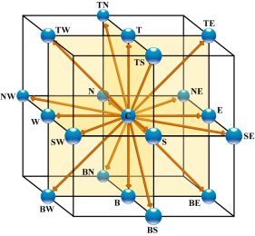
Figure 1: The workhorse lattices in two and three dimensions, with $9$ and $19$ discrete velocities, respectively.

The left hand side of eq. (2) denotes free-streaming, while the right hand side is the collision step, which consists of a short-range component, driving the system towards a local equilibrium $f_{i}^{eq}$ and a soft-core source of momentum $S_{i}(\vec{x};t)$. The latter is in fact more general and can represent the source of any macroscopic quantity relevant to the physics in point. This is a major asset of LB, one that permits to include complex mesoscale physics often beyond the realm of continuum fluids, at a minimum cost in terms of programming and computing overheads.

The local equilibrium corresponds to a finite-order truncation of a local Maxwellian:

$$f_{i}^{eq}=w_{i}\rho(1+\beta u_{i}+\frac{\beta^{2}}{2}q_{i})$$ (3)

where $\beta=1/c_{s}^{2}$, $u_{i}=\vec{u}\cdot\vec{c}_{i}$ and $q_{i}=u_{i}^{2}-u^{2}c_{s}^{2}$, $c_{s}$ and $\vec{u}$ being the lattice sound speed and the local flow velocity, respectively. In the above $w_{i}$ is a set of weights normalized to unity, the discrete analogue of the absolute Maxwellian in continuum velocity space. The truncation is an unavoidable consequence of lattice discreteness, which permits to recover Galilean invariance only to a finite order in the Mach number $Ma=|\vec{u}|/c_{s}$. The relevant hydrodynamic quantities are computed as simple linear and local combinations of the discrete distributions, namely:

$$\rho(\vec{x};t)=\sum_{i}f_{i}(\vec{x};t),\;\;\;\rho\vec{u}(\vec{x};t)=\sum_{i}\vec{c}_{i}f_{i}(\vec{x};t)$$ (4)

where $\rho$ is the fluid density. Higher order moments deliver the fluid pressure and stress tensor in the form of linear and local combinations of the discrete populations, which proves very convenient for simulation purposes. Formally, The LB eq. (2) is nothing but a set of finite-difference equations, and yet one with great power inside. This power stems mainly from four basic ingredients, namely: i) Exact free-streaming, ii) Local lattice equilibria, iii) Tunable relaxation matrix, iv) Flexible external source, Before moving on to these items, we hasten to add that the eq. (2) can be shown to converge to the (quasi-incompressible) Navier-Stokes equations in the usual limit of small Knudsen numbers, $Kn=\lambda/L\ll 1$, i.e. small mean free path versus the typical scale of variation of hydrodynamic quantities. This is also a statement of weak departure from local equilibrium. Technically, this entails a Taylor expansion in the lattice time step, as combined with a double expansion in low Knudsen and Mach number. The tool of the trade is the Chapman-Enskog asymptotics [28].

5 Mainstream LB applications

As mentioned above, at the time of this writing LB is a massive bibliographic presence in fluid dynamics and most allied fields, particularly soft flowing matter [6] and the physics/biology interface [29]. It would be utterly impossible to cover this vast ground in any single paper, hence here we shall just outline the main applications in very broad strokes.

5.1 Macroscopic flows

Historically, Lattice Boltzmann was developed as a computational alternative to the discretization of the Navier-Stokes equations of continuum fluid dynamics, the main target being high-Reynolds turbulent flows in complex geometries [30]. The initial hopes were that LB would offer a better resolution of the near-grid scales or even provide a natural subgrid model via the extra degrees of freedom of the kinetic representation (then dubbed ”ghost modes”) versus the hydrodynamic one [31].

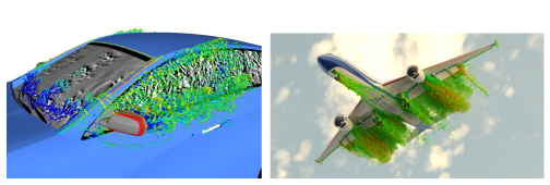
Figure 2: Two examples of fully-turbulent lattice Boltzmann simulations for automotive and aeronautical applications. (Courtesy of Dassault Systemes)

This turned out not to be the case, but prepared the ground for subsequent developments which have met with significant success, as witnessed by existence of a number of open source [32] and commercial codes, particularly POWERFLOW, developed by EXA Corporation and recently acquired by Dassault Systemes [33]. The academic side has also witnessed remarkable progress, mostly but not exclusively in connection, with the development of the entropic method [34] and Large-Eddy simulations [35, 36, 37]. More recently, LB has also been used to study turbulent flows with suspended bodies, a topic of great relevance for energy and environment [38]. Another successful application of LB to macro-hydrodynamics are flows in porous media, with accompanying heterogeneous chemical reactions [39, 40], which draw major benefits from the LB ability to deal efficiently with grossly irregular geometries.

5.2 Multiphase and colloidal flows

Two areas where LB has made a real difference are multiphase/multi-component flows and flows with suspended bodies [41]. In the former case LB offers the major benefit of simplicity: interfaces need no explicit tracking but emerge spontaneously, informed by the corresponding mesoscale forces which are implemented as soft source terms. This benefits comes at the prize of several limitations, most of which have been however significantly mitigated in the course of time [42, 43, 44].

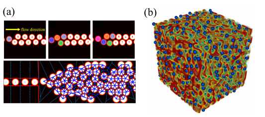
Figure 3: (a) Spontaneous ordering of droplets in a microfluidic channel ([48]). (b) Large-scale simulation of a colloidal flow ([50])

Many LB variants exist today which have found massive use especially in the area of microfluidics (see below). Among these, a very fruitful option is offered by the Color Gradient technique [45], in which the idea is to add an explicit anti-diffusive flux sending particles of each species uphill along their density gradient instead of against it, thereby promoting the formation of an interface against the coalescing effect of surface tension. The stress-jump condition across fluid interfaces can be further augmented with an immersed-like force modeling the repulsive effect generated by a surfactant solution absorbed onto the drop interfaces. This contribution can be added to the collision operator via a suitable forcing term as proposed in [46, 47]. The above approach has been shown to correctly capture highly non trivial many-droplet configurations, like dense emulsions and foams. As an example, the extended multi-component model has been shown to reproduce the formation of ordered droplets clusters in microfluidic channels [48]. As shown in figure 3(a), the droplets, continuously injected within the main channel, undergo a spontaneous ordering into hexagonal clusters, which is due to a subtle competition between local, short-range, repulsive interactions (i.e., the near-contact forces) and the surface tension. Another major field of application are complex flows with immersed bodies, both rigid and deformable, in which LB is typically coupled to other methodologies for fluid structure interactions [41, 49]. To this regard, recent Multi-GPU state-of-the art implementations of LB codes for multi-component colloidal flows [50] have been shown to deliver remarkable performances, up to $200$ GLUPS (Giga Lattice Updates Per Second on a cluster made of $512$ A100 NVIDIA cards), on computational grids with several billions of lattice points ( see figure 3(b). These results open attractive prospects for the computational design of new materials based on colloidal particles.

5.3 Micro and nano-hydrodynamics

In the early 1990’s LB was applied exclusively to macroscopic fluid problems, and even with a vengeance, since some prominent researchers vetoed its use for anything but this [51]. Yet, precisely in those years, a few groups offered numerical evidence that the LB scheme can handle moderately non-equilibrium flows beyond the strict realm of hydrodynamics [52, 53, 55]. This, together with a boost of activity in the area of non-ideal, multiphase and multicomponent fluids, has led to a major mainstream of LB applications, mostly in soft-matter and microfluidics [46, 56, 57, 58, 59, 60, 61, 62].

The key ingredients for this transition from the macro to the micro-hydrodynamic levels turned out to be the introduction of higher order lattices, securing the compliance with generalized hydrodynamics beyond the Navier-Stokes description, as well as the development of suitable boundary conditions, capable of dealing with non-equilibrium effects associated with large gradients at solid walls [53, 54]. Very recently, the LB has also been successfully coupled to off-lattice, particle models to develop novel classes of fully mesoscale hybrid approaches capable of capturing the physics of fluids at the micro‐ and nanoscales whenever a continuum representation of the fluid falls short of providing the complete physical information. In addition, LBM has also been coupled to Direct Simulation Monte Carlo (DSMC) in view of efficiently simulating isothermal flows characterized by variable rarefaction effects [63].

Another major mainstream of current LB research is the study of flows with suspended bodies, both rigid and deformable ones. This was originated by pioneering work on colloidal nanoflows, i.e. rigid spheres flowing in a LB solvent, which was sparked by the development of the so-called fluctuating Lattice Boltzmann, taking in due account the statistical fluctuations which characterize hydrodynamic behavior at the nanoscale [64].

The original fluctuating LB (FLB) scheme for colloidal flows has spawn many subsequent developments, including biopolymers and deformable objects of biological interest, such as membranes and cells. Methodologically, this was made possible by the fruitful merge between LB and the Immersed Boundary Method [49]. Details of this highly technical and utterly important subject can be found in [41].

6 Quantum-relativistic fluids

Even though the mainstream of LB research remains hard-rooted it classical physics, it should be mentioned that the LB scheme is amenable to remarkable generalizations in the direction of both quantum and relativistic mechanics. The former possibility was recognized as early as 1993, building on a formal analogy between the Boltzmann equations and the Dirac equation of relativistic quantum mechanics [65, 66, 67]. Incidentally, the corresponding quantum LB (QLB) scheme was later shown to represent a quantum random walk, as per the seminal Ahronov et al paper, which appeared just a couple of months ahead of QLB. The QLB was also shown to be amenable to quantum computing [68].

The extension of the LB scheme to relativistic fluids came much later, as it dates of 2010 [69, 70] and it has undergone major progress in the last decade [71]. The relativistic LB requires some non-trivial technical manipulation due to the fact that, unlike the Newtonian case, the relativistic energy of massive particles is an irrational function of the particle momentum, i.e.

$$E(p)=\sqrt{m^{2}c^{4}+p^{2}c^{2}}$$ (5)

This makes the task of developing discrete-velocities schemes less straightforward than in the non-relativistic case, $E\ll mc^{2}$, because one can no longer rely on orthogonal polynomials in the continuum, such as Hermite’s. However, suitable discrete orthogonalization techniques have been developed over the years, which have permitted to realize fairly efficient relativistic LB schemes despite the large number of discrete speeds involved [72].

This has permitted the simulation of relativistic flows, such as electron transport in graphene and transport phenomena in quark gluon plasmas. Amazingly, similar schemes have also been used for the simulation of cosmic neutrinos in astrophysical flows [26]. Relativistic hydrodynamics is still a small niche as compared to the massive activity in non-relativistic fluids. However, due to the mounting interest in relativistic fluids at the crossroads between condensed matter, high-energy physics and gravity [73], it is reasonable to expect that relativistic LB schemes may gain significant momentum for the years to come.

7 Towards exascale LB

A common thread to all the LB applications is their outstanding amenability to parallel computing, across virtually any kind of architecture (provided hard and ingenuous implementation work is spent on the task). Remarkable examples abound in the literature [32, 74, 75, 76, 77, 78, 79, 80, 81], but here I shall just refer to two instances I am directly familiar with.

Figure 4: LB across scales: from above galaxies all the way down inside the proton! Top row: astrorelativistic jets resulting from binary neutron star mergers, flow around a racing car, blodd flow in human arteries at blood cell resolution. Middle: a wet foam. Bottom row: double-stranded biopolymer trasnslocating through a membrane, The electronic cloud around the methane molecule, the quark-gluon plasma produced by heavy ion collisions. All of these flows, covering from megaparsecs to femtometers (37 decades), made use of different variants of the LB method.

First, the use LB as a fast water solvent solver for the study of protein crowding within the cell, which reached in excess of 20 Pflops on the Titan supercomputer, but many outstanding performances have been obtained in other massively parallel applications at all scales of motion [76]. As a recent and rather spectacular example, I wish to quote the full-scale simulation of the deep-sea sponge Euplectella Aspergillum, with a fully realistic description of the highly complex geometrical porous structure at a 10-micron resolution, all the way up to the centimeters of the full sponge [82]. It is fair to say that such kind of study would have been impossible without LB. The above applications witness the ability of suitably optimized LB codes to achieve Petascale performance on highly non-trivial fluid problems.

The LB assets, exact free streaming, machine-accurate conservative collisions and flexibility towards inclusion of mesoscale physics are expected to carry over from the Peta to the Exascale.

However,taking LB towards the exascale will face the usual challenges common to most numerical methods, namely the need of minimizing the cost of accessing data [83], offsetting communication overheads by overlapping communication and computation and, a possibility unexplored so far to the best of this author’s knowledge, develop fault-tolerant LB schemes. All of the above, by taking into account the increasing constraints on power consumption, for which machine learning might prove a valuable ally, typically by optimizing the reconstruction of fine-grained information from coarse-grain simulations.

8 Towards LB Quantum Computing

Quantum computing holds great promises to become the leading simulation technology for the future. To make the promise come true, however, several obstacles need to be circumvented, on both hardware and software fronts. As to latter, one has first to identify the class of problems which can be formulated in terms of quantum computing algorithms. To date, the most likely candidates for such a paradigm shift are mostly in the area of quantum chemistry and material science; understandably so, since quantum computing is obviously most suited to quantum systems [84]. In this respect, fluid dynamics faces with two major issues: it is strongly nonlinear and dissipative. Indeed, quantum computing for fluids is still in its infancy [85, 86], even though interesting efforts to circumvent the two major barriers have started to emerge in the recent years. In the following we just sketch the basi ideas.

8.1 Handling nonlinearity

As to nonlinearity, an interesting possibility is to advocate Carleman linearization, which consists in trading non-linearity for linearity in extra-dimensions.

A simple example says it best.

Consider the logistic equation:

$$\frac{dx}{dt}=x(1-x)$$ (6)

with the initial condition $x(0)=1/2$.

The quadratic non-linearity can be formally disposed of by defining two independent variables $x_{1}\equiv x$ and $x_{2}\equiv x^{2}$, so that the quadratic logistic equation becomes formally linear, i.e.:

$$\frac{dx_{1}}{dt}=x_{1}-x_{2}$$ (7)

This is obviously open and requires an additional equation for $x_{2}$. By differentiating $dx^{2}/dt=2xdx/dt=2x^{2}(1-x)$ and defining $x_{3}\equiv x^{3}$, we obtain

$$\frac{dx_{2}}{dt}=2x_{2}-2x_{3}$$ (8)

This is still open , as it requires an additional equation for $x_{3}$. It is therefore apparent that teh Carleman linearization is confronted with an endless hierarchy which needs to be truncated at some stage.

The first order truncation is $x_{2}=0$, which delivers $x(t)=e^{t}$, just the initial stage of the exact solution of the logistic equation, $x(t)=e^{t}/(1+e^{t})$. The second order truncation is $x_{3}=0$, delivers a $2\times 2$ linear system, whose solution is readily checked to be $x(t)=e^{t}(1-e^{t})$, still not quite exact but closer than the previous one. The name of the game is quite clear: by truncating the Carleman series at level $N$ we obtain a $N\times N$ system of first order linear ODEs, whose solution captures the $N$-th order expansion of the denominator in the exact solution. Clearly, the exact solution, meaning by this a solution which holds exactly and at arbitrarily long times, can only be recovered in the limit $N\to\infty$. Hence the Carleman linearization buys linearity, but at the price of an inevitable error which grows in time. Preliminary results indicate that the truncation error decays fast with the order of truncation [87], but much more work is required to put this observation on a solid basis for the actual LB equation. This is certainly a most intersting direction for future research.

8.2 Handling Dissipation

Several techniques are available to handle dissipative effects within a conservative (Hamiltonian) formulation. One possibility is to augment the original dissipative system with one (or more) extra-variables, call it reservoir, absorbing the dissipated energy so that the global system, original plus reservoir, is by construction conservative.

Another possibility is to represent dissipative operators (the collision operator in the case of LB) as the weighted sum of two unitaries. Let $C_{ij}$ the Carleman-linearized collision matrix associated with the LB scheme, one writes

$$C_{ij}=U_{ij}+\alpha V_{ij}$$ (9)

where $U$ and $V$ are two unitaries and $\alpha$ a numerical factor between $0$ and $1$. The price for splitting the Carleman matrix into the sum of two unitaries is that the quantum update may eventually fail, with a probability which depends on $\alpha$. For the case of linear advection-diffusion problems, it has been shown that the loss of efficiency can be contained to some 10 percent on a wide range of $\alpha^{\prime}s$ [88]. Whether the same is true for the full fluid equations is a totally open question at the time of this writing, and again an interesting topic for future research.

9 Summary: Whither LB?

As we have been illustrating in this short review, over the last three decades, the LB has made proof of an amazingly flexibility, with a wide spectrum of applications covering fluid motion across an impressively broad range of scales, literally from inside protons to the outer Universe (see figure 4)! The impact on CFD and allied fields is massive, as reflected by its bibliographic indicators. But even leaving aside from bibliometrics, it is fair to say that LB has greatly facilitated the inspection of highly complex flowing states of matter which would be very hard to analyze with other methods, if possible at all. The main asset behind this success is always the same: information travels along straight characteristics and the streaming step is literally exact (zero-roundoff). With the due amount of work, far from trivial in the case of complex geometries, this permits to achieve high parallel efficiencies also in the presence of fairly complex geometries and strong nonlinearities. In the end, this is what makes LB such a powerful tool for the study of complex states of flowing matter across regimes and scales. This said, many challenges still remain. Among others, how to control lattice artifacts in high-Reynolds fluid flows with immersed bodies; how to enhance the stability of LB schemes in the presence of substantial heat transfer and compressibility effects; how to handle large density contrasts in multiphase flows. How to represent large nanoscale fluctuations without hampering numerical stability. From a more technical, but no less important, perspective, how to make LB compliant with the forthcoming exascale architectures, which requires a serious effort in the direction of minimizing the cost of accessing data [79, 80, 83]. And as mentioned above, how to make LB compliant with the (hopefully) forthcoming quantum computing architectures. Summarizing, the original Lattice Gas idea of solving fluid dynamics by means of fictitious molecules instead of discretizing continuum equation did not work in its original and most radical (boolean) form. However, it has proved exceedingly fruitful from the conceptual standpoint, by providing the stepping stone for a new class of mesoscale methods and particularly the Lattice Boltzmann method. In hindsight, LB could have been derived as a discrete velocity version of the continuum Boltzmann equation, with no reference to any microscale dynamics. However, this does not change the fact that, without the LGCA inspiration, LB would have been discovered much later, if at all.

10 Acknowledgments

This research has received funding from the European Research Council under the Horizon 2020 Programme Grant Agreement n. 739964 (”COPMAT”). The author is indebted to very many colleagues and friends in Italy and around the world, too many to mention without taking the chance of embarrassing omissions. Here I only wish to thank Andrea Montessori and Mihir Durve for their generous help in putting this manuscript together.

References

- [1] U. Frisch, B. Hasslacher and Y. Pomeau, Phys. Rev. Lett. 56, 1505, (1986)
- [2] S. Wolfram, J. Stat. Phys. 45, 471, (1986)
- [3] P.J. Hills, The Washington Post, Nov 19, 1985
- [4] M. Henon, Complex Systems 1, 763 (1987), https://content.wolfram.com/uploads/sites/13/2018/02/01-4-12.pdf
- [5] S. Succi, The lattice Boltzmann equation for fluid dynamics and beyond, Oxford Univ. Press (2001)
- [6] S. Succi, The lattice Boltzmann equation for complex states of flowing matter, Oxford Univ. Press (2018)
- [7] C. Aidun and J. Clausen, Annu. Rev. Fluid Mech, 42, 439, (2010)
- [8] J.E. Broadwell, Phys. Fluids , 7 1243–1247 (1964) R. Gatignol, ”Théorie cinétique d’un gaz répartition discrète de vitesses” , Springer (1975); R. Monaco, L. Preziosi, ”Fluid dynamic applications of the discrete Boltzmann equation” , World Sci. (1991) T. Platkowski, R. Illner, survey on the mathematical aspects of the theory” SIAM Review , 30 (2) 213–255 (1988)
- [9] G. Mc Namara and G. Zanetti, Phys. Rev. Lett., 61, 2332, (1988)
- [10] F. Higuera and S. Succi, Europhys. Lett. ,8, 517, (1989). For the record, the seeds of the EPL paper can be found in F. Higuera, in Discrete Kinetic Theory, Lattice Gas Dynamics and Foundations of Hydrodynamics, R. Monaco ed., World Scientific, Singapore, p. 162 1989 and S. Succi, R. Benzi, F. Higuera, ibidem, p. 329.
- [11] F. Higuera and J. Jimenez, Europhys. Lett., 9, 663, (1989)
- [12] F. Higuera , S. Succi and R. Benzi, Europhys. Lett., 9, 345, (1989)
- [13] R. Benzi, S. Succi and M. Vergassola, Phys. Rep., 222, 145, (1992)
- [14] H. Chen, S. Chen and W. Matthaeus, Phys. Rev. A, 45, R5342 (1992)
- [15] S. Chen, H. Chen et al, Phys. Rev. Lett., 67(27), 3776, (1991)
- [16] J. M. Koelman, Europhys. Lett., 15(6), 603, (1991)
- [17] Y. Qian, D. d’Humières and P. Lallemand, Europhys. Lett., 17(6), 479, (1992)
- [18] D. d’Humieres, I. Ginzburg, M. Krafczyk et al. Phil. Trans. Roy. Soc., 360,437, (2002)
- [19] I. Karlin, A. Ferrante and H. C. Oettinger, Europhys. Lett.,62(3), (1999)
- [20] X. He and L.S. Luo, Phys. Rev. E. 56, 6811, (1997)
- [21] Z. Guo, C. Zheng and B. Shi, Phys. Rev. E, 65, 046308 (2002)
- [22] S. Succi, Eur. Phys. J. B: 64, 471 (2008)
- [23] F. Alexander, S. Chen, JD Sterling, Phys. Rev. E, 47, R2249, (1993)
- [24] X. He, S. Chen, G. Doolen, J. Comp. Phys., 146, 282 (1998)
- [25] M. Sbragaglia et al, J. Fluid Mech., 628, 299, (2009)
- [26] L.R. Weih, A. Gabbana, D. Simeoni, L. Rezzolla, S. Succi, R. Tripiccione, MNRAS, 498, Issue 3 (2020).
- [27] S. Succi, EPL Perspective, 109, 5, 50001 (2015)
- [28] S. Chapman and T. Cowling, The mathematical theory of non-uniform gases, Cambridge U.P., (1990)
- [29] S. Succi, Sailing the Ocean of Complexity: Lessons from the Physics-Biology Frontier, Oxford U.P., (2022)
- [30] H. Chen et al, Science, 301, 633, (2003)
- [31] Benzi, R., Succi, S., Two-dimensional turbulence with the lattice Boltzmann equation, Journal of Physics A: Mathematical and General, 23(1), L1 (1990).
- [32] Latt, J., Malaspinas, O., Kontaxakis, D., Parmigiani, A., Lagrava, D., Brogi, F., …, Chopard, B. Computers and Mathematics with Applications, 81, 334-350 (2022)
- [33] https://www.3ds.com/products-services/simulia/products/powerflow/
- [34] S.S. Chikatamarla, C.E. Frouzakis, I.V. Karlin et al. J. Fluid Mech. 656, 298, (2010)
- [35] O. Malaspinas, P. Sagaut, Journal of Fluid Mechanics 700, 514-542 (2010) Toward advanced subgrid models for Lattice-Boltzmann-based Large-eddy simulation: Theoretical formulations
- [36] P Sagaut, Computers and Mathematics with Applications 59 (7), 2194-2199, (2010)
- [37] NH Maruthi, C Thantanapally, M Namburi, V Kumaran, S Ansumali, arXiv preprint arXiv:2204.02191(2022)
- [38] Perlekar, P., Biferale, L., Sbragaglia, M., Srivastava, S., Toschi, F. Physics of Fluids, 24(6), 065101.
- [39] Q. Kang, P. Lichtner, DR Janecky, Advances in Applied Mathematics and Mechanics 2(5):545-563 (2010)
- [40] G Falcucci, S Succi, A Montessori, S Melchionna, P Prestininzi, C Barroo, … Microfluidics and Nanofluidics 20 (7), 1-13
- [41] T. Kruger, The Lattice Boltzmann Method, Springer Verlag (2017)
- [42] X. Shan and H. Chen, Phys. Rev. E 47, 1815, (1993)
- [43] M. Swift et al, Phys. Rev. Lett., 75, 830, (1995)
- [44] G. Falcucci et al., Comm. in Comp. Phys., 9, 269, (2011)
- [45] Gunstensen, A. K., Rothman, D. H., Zaleski, S. and Zanetti, G. Physical Review A, 43(8), 4320 (1991)
- [46] A Montessori, M Lauricella, N Tirelli, S Succi, J. of Fluid Mech. 872, 327-347, (2019)
- [47] Montessori, A., Tiribocchi, A., Lauricella, M., Bonaccorso, F. and Succi, S. Physical Review Fluids, 6(2), 023606 (2020).
- [48] Montessori, A., Tiribocchi, A., Lauricella, M., Bonaccorso, F. and Succi, S. Soft Matter, 17(9), 2374-2383 (2021).
- [49] Zhi-Gang Feng, E. Michaelides, J. of Comp. Phys. 195, 602, (2004)
- [50] Bonaccorso, F., Lauricella, M., Montessori, A., Amati, G., Bernaschi, M., Spiga, F., Tiribocchi A. and Succi, S. , arXiv preprint arXiv:2112.08264 (2021).
- [51] L.S. Luo, Phys. Rev. Lett. 92, 139401 (2004)
- [52] X. Shan, X. Yuan and H. Chen, J. Fluid Mech., 550, 413, (2006)
- [53] S. Ansumali and I.V. Karlin, Phys. Rev. E, 66, 026311 (2002)
- [54] S.P. Thampi, S. Ansumali, R. Adhikari, Sauro Succi, J. Comp. Phys., 234, 1, (2013)
- [55] A. Montessori, P. Prestininzi, M. La Rocca, S. Succi, Phys. Rev. E 92 (4), 043308, (2015)
- [56] B. Duenweg and A. Ladd, Adv. Polym. Sci., 221, 89, (2009)
- [57] M. Sbragaglia et al, Phys. Rev. Lett. 97, 204503(2006)
- [58] M. Sbragaglia et al, Phys. Rev. E 75, 026702 (2007)
- [59] J. Latt and B. Chopard, Math. Comput. Simul., 72, 165 (2006)
- [60] XD Niu et al, Phys. Rev. E 76, 036711, (2007)
- [61] R. Benzi, L. Biferale, M. Sbragaglia, S. Succi, F.Toschi, EPL (Europhys. Lett.) 74(4) 651, (2006)
- [62] A Tiribocchi, A Montessori, M Lauricella, F Bonaccorso, S Succi, S Aime, et al, Nat. Commun. 12 (1), 1-10, (2021)
- [63] Di Staso, G., Clercx, H. J. H., Succi, S., Toschi, F. . Journal of Computational Science, 17, 357-369 (2016)
- [64] A. Ladd, J. Fluid Mech., 271, 285 (1994),
- [65] S. Succi and R. Benzi, Physica D 69, 327, (1993)
- [66] P. Dellar, D. Lapitski, Phil. Trans. Roy. Soc., 369, 2155 (2011)
- [67] F. Fillion et al, Phys. Rev. Lett. 111, 160602, (2013)
- [68] J. Yepez et al., Phys. Rev. Lett. 103, 084501 (2009)
- [69] M. Mendoza et al, Phys. Rev. Lett., 105, 014502, (2010).
- [70] M. Mendoza, H.J. Herrmann and S. Succi, Phys. Rev. Lett., 106, 156601, (2011).
- [71] A. Gabbana, D. Simeoni, S. Succi, R. Tripiccione, Phys. Rep., 7 (2020).
- [72] A. Gabbana, V. Ambrus D. Simeoni, S. Succi, R. Tripiccione, Nat. Comp. Sci, in press (2022)
- [73] G. Policastro, D.T. Son and A. Starinets, Phys. Rev. Lett., 87, 081601, (2001)
- [74] M Bernaschi, S Melchionna, S Succi, M Fyta, E Kaxiras, JK Sircar Computer Physics Communications, 180 (9), 1495-1502 (2009)
- [75] M Bernaschi, M Fatica, S Melchionna, S Succi, E Kaxiras Concurrency and computation: practice and experience 22 (1), 1-14 (2010)
- [76] M. Bernaschi, M. Bisson, M. Fatica and S. Melchionna, Proceedings of the International Conference on High-Performance Computing, Networking, Storage and Analysis (2013).
- [77] MD Mazzeo, PV Coveney Computer Physics Communications 178 (12), 894-914 (2008)
- [78] Feichtinger, C., Donath, S., Köstler, H., Götz, J., Rüde, U. , Journal of Computational Science, 2(2), 105-112 (2013).
- [79] S Alowayyed, D Groen, PV Coveney, AG Hoekstra Journal of Computational Science 22, 15-25 (2017)
- [80] S Succi, G Amati, M Bernaschi, G Falcucci, M Lauricella, A Montessori Computers and Fluids 181, 107-11 (2019)
- [81] https://walberla.net
- [82] G Falcucci, G Amati, P Fanelli, VK Krastev, G Polverino, M Porfiri, S Succi, Nature 595 (7868), 537-541, (2021)
- [83] Shet, A. G., Sorathiya, S. H., Krithivasan, S., Deshpande, A. M., Kaul, B., Sherlekar, S. D., Ansumali, Physical Review E, 88(1), 013314 (2013).
- [84] R. Feynman, International Journal of Theoretical Physics volume 21, pages 467–488 (1982)
- [85] F. Gaitan, npj Quantum Information 6:61(2020) ; https://doi.org/10.1038/s41534-020-00291-0
- [86] Jin-Peng Liu , Herman Kolden Hari K. Krovi, Nuno F. Loureiro, Konstantina Trivis and Andrew M. Childs, PNAS 2021 Vol. 118 No. 35 e2026805118(2021), https://doi.org/10.1073/pnas.2026805118
- [87] W. Itani and S. Succi, Fluids, 7, 1(24), (2022)
- [88] A. Mezzacapo, M Sanz, L Lamata, IL Egusquiza,S. Succi and E. Solano, Nat. Sci. Comp. , 5, 1,1(2016)