IFISS3D: A computational laboratory for investigating finite element approximation in three dimensions

Abstract.

IFISS is an established MATLAB finite element software package for studying strategies for solving partial differential equations (PDEs). IFISS3D is a new add-on toolbox that extends IFISS capabilities for elliptic PDEs from two to three space dimensions. The open-source MATLAB framework provides a computational laboratory for experimentation and exploration of finite element approximation and error estimation, as well as iterative solvers. The package is designed to be useful as a teaching tool for instructors and students who want to learn about state-of-the-art finite element methodology. It will also be useful for researchers as a source of reproducible test matrices of arbitrarily large dimension.

1. Introduction and brief history

The IFISS software [15] was developed by Elman, Ramage and Silvester [7]. It can be run in MATLAB (developed by the MathWorks^©) or Gnu Octave (free software). It is structured as a stand-alone package for studying discretisation algorithms for partial differential equations (PDEs), and for exploring and developing algorithms in numerical linear and nonlinear algebra for solving the associated discrete systems. It can be used as a pedagogical tool for studying these issues, or more elementary ones such as the properties of Krylov subspace iterative methods. Investigative numerical experiments in a teaching setting enable students to develop deduction and interpretation skills, and are especially useful in helping students to remember critical ideas in the long term. IFISS is also an established starting point for developing code for specialised research applications (as evidenced by the variety of citations to it, see [16]), and is extensively used by researchers in numerical linear algebra as a source of reproducible test matrices of arbitrarily large dimension.

The development of the MATLAB functionality during the period 1990–2005 opened up the possibility of creating a problem-based-learning environment (notably the IFISS package) that could be used together with standard teaching mechanisms to facilitate understanding of abstract theoretical concepts. The functionality of IFISS was significantly extended in the period between 2005 and 2015—culminating in the publication of the review article [8], which coincided with the publication of the second edition of the monograph [9].

A unique feature of IFISS is its comprehensive nature. For each problem it addresses, it enables the study of both discretisation and iterative solution algorithms, as well as the interaction between the two and the resulting effect on solution cost. However, it is restricted to the solution of PDEs on two-dimensional spatial domains. This limitation can be overcome by adding the new IFISS3D toolbox [12] to the existing IFISS software. The three-dimensional finite element approximation and error estimation strategies included in the new software are specified in the next section. Section 3 describes three reference problems that provide a convenient starting point for studying rates of convergence of the approximations to the true solution. The structure of the IFISS3D package is discussed in Section 4. The directory structure is intended to simplify the task of extending the functionality to other PDE problems and higher-order finite element methods. Case studies of two important aspects of three-dimensional finite element approximation are presented in Section 5.

2. Discretisation and Error Estimation Specifics

The IFISS3D software generates approximations to the solution of PDEs modelling physical problems in three spatial dimensions. The starting point for the process is a finite element partitioning of a domain of interest $D\subset\mathbb{R}^{3}$ into $n_{e}$ hexahedral (brick) elements $\square_{e}\subset D$, $e=1,2,3,\ldots,n_{e}$ so that

$$\begin{cases}\square_{e}\ \text{is open in}\ \mathbb{R}^{3}\\ D=\overline{\cup_{e=1}^{n_{e}}\square_{e}}\\ \square_{i}\cap\square_{j}=\emptyset,\ \ i\neq j,\end{cases}$$

where the upper bar represents the closure of the union. An arbitrary element $\square_{e}$ is a hexahedron with six faces and with local vertex coordinates $(x^{e}_{i},y^{e}_{i},z^{e}_{i})$, $i=1,2,\ldots,8$ ordered as shown in Fig. 1.

Figure 1. Hexahedral (brick) element (a) vertex numbering and (b) face numbering.

The simplest choice of a conforming finite element space in $\mathbb{R}^{3}$ is the $\mathbb{Q}_{1}$ approximation space of piecewise trilinear polynomials that take the form

$$q_{1}^{e}(\boldsymbol{x})=(\alpha_{1}x+\alpha_{2})(\alpha_{3}y+\alpha_{4})(\alpha_{5}z+\alpha_{6})$$

on each element $\square_{e}$. The continuity of the global approximation is ensured by defining a Lagrangian basis for $q^{e}_{1}$ at the eight vertices of the hexahedron, that is

$$\phi^{e}_{i}(\boldsymbol{x})=\begin{cases}1&\text{if}\ \ x=x^{e}_{i},y=y^{e}_{i},\ z=z^{e}_{i},\\ 0&\text{at the other vertices}\end{cases},\quad i=1,2,\ldots,8.$$

Figure 2. Isoparametric mapping from a reference cube.

Additional geometric flexibility (stretched grids) can be incorporated by constructing an isoparametric transformation from the reference cube $[-1,1]^{3}$ (denoted $\square_{\star}$) to a general hexahedron $\square_{e}$. To this end we define the following basis functions for the reference element

$$\ell^{i}(\xi,\eta,\zeta)=1/8(1+\xi_{i}\xi) (1+\eta_{i}\eta)(1+\zeta_{i}\zeta),\quad i=1,2,\ldots,8$$

where $\xi_{i},\eta_{i},\zeta_{i}$ are node values of $\square_{\star}$ and $\xi,\eta,\zeta\in[-1,1]$ and map to an arbitrary hexahedral element $\square_{e}$ with vertices $(x^{e}_{i},y^{e}_{i},z^{e}_{i})$, $i=1,2,\ldots,8$ by the change of variables

$$x(\xi,\eta,\zeta)=\sum_{i=1}^{8}x^{e}_{i}\ell^{i}(\xi,\eta,\zeta),\ y(\xi,\eta,\zeta)=\sum_{i=1}^{8}y^{e}_{i}\ell^{i}(\xi,\eta,\zeta),\ z(\xi,\eta,\zeta)=\sum_{i=1}^{8}z^{e}_{i}\ell^{i}(\xi,\eta,\zeta).$$

This mapping is illustrated in Fig. 2.

The IFISS3D software also provides the option of higher-order approximation using polynomials that are globally continuous but piecewise triquadratic ($\mathbb{Q}_{2}$), that is,

$$q_{2}^{e}(\boldsymbol{x})=(\alpha_{1}x^{2}+\alpha_{2}x+\alpha_{3})(\alpha_{4}y^{2}+\alpha_{5}y+\alpha_{6})(\alpha_{7}z^{2}+\alpha_{8}z+\alpha_{9}).$$

The continuity of the global $\mathbb{Q}_{2}$ approximation is ensured by defining a Lagrangian basis for $q_{2}^{e}$ at the eight vertices of the hexahedron together with the nineteen additional nodes shown in Fig. 3.

Figure 3. (a) $\mathbb{Q}_{1}$ nodes and numbering and (b) $\mathbb{Q}_{2}$ nodes and numbering.

The $\mathbb{Q}_{2}$ isoparametric transformation is given by

$$x(\xi,\eta,\zeta)=\sum_{i=1}^{27}x^{e}_{i}{\psi}^{i}(\xi,\eta,\zeta),\quad y(\xi,\eta,\zeta)=\sum_{i=1}^{27}y^{e}_{i}{\psi}^{i}(\xi,\eta,\zeta),\quad z(\xi,\eta,\zeta)=\sum_{i=1}^{27}z^{e}_{i}{\psi}^{i}(\xi,\eta,\zeta),$$

with reference basis functions

$${\psi}^{i}(\xi,\eta,\zeta)={N}^{k}(\xi)\,{N}^{l}(\eta)\,{N}^{m}(\zeta),\ i=1,2,\ldots,27;\ k,l,m=1,2,3$$

where

$${N}^{1}(\xi)=1/2(\xi-1)\xi,\ {N}^{2}(\xi)=1-\xi^{2},\ \ {N}^{3}(\xi)=1/2(1+\xi)\xi.$$

A fundamental feature of the IFISS software is the use of hierarchical error estimation. This strategy was developed for scalar elliptic PDEs by Bank & Smith [1], but has been extended to more general PDE problems (including systems of PDEs) over the past two decades. Crucially, the hierarchical approach yields reliable estimates of the error reduction that can be expected using an enhanced approximation. It also provides a rigorous setting for establishing the convergence of adaptive refinement strategies, such as those that are built into the T-IFISS package [2], and the ML-SGFEM software [5] associated with the work of Crowder et al. [6] on multilevel stochastic Galerkin finite element methods for parametric PDEs.

A posteriori error estimation in practical finite element software (such as DUNE [3] or FEniCS [11]) is typically done using residual error estimation strategies. This requires the computation of norms of PDE residuals in the interior of each element and norms of flux jumps (edge residuals) on inter-element faces. The additional computational cost of hierachical error estimation is nontrivial. Having generated a solution using $\mathbb{Q}_{1}$ approximation, computed interior and edge residuals are input as source data for element PDE problems that are solved numerically using an enhanced approximation space. In IFISS3D, one can construct the enhanced space using triquadratic basis functions on the original element $(\mathbb{Q}_{2}(h))$, or trilinear basis functions defined on a subdivision of the original element into 8 smaller ones $(\mathbb{Q}_{1}(h/2))$. These basis or ‘bubble’ functions are associated with the white nodes illustrated in Fig. 4(a), leading to linear algebra systems of dimension nineteen. Alternatively, reduced versions of these spaces of dimension 7, denoted $\mathbb{Q}^{r}_{2}(h)$ and $\mathbb{Q}^{r}_{1}(h/2)$, can also be constructed by incorporating only the basis functions associated with the interior node and the central nodes on each face, as illustrated in Fig. 4(b). In all four cases, a low-dimensional system must be solved for every element in the mesh. This calculation is efficiently vectorised in IFISS.

Figure 4. White nodes associated with bubble functions used to construct (a) full $\mathbb{Q}_{2}(h)$ or $\mathbb{Q}_{1}(h/2)$ and (b) reduced $\mathbb{Q}^{r}_{2}(h)$ and $\mathbb{Q}^{r}_{1}(h/2)$ error estimation spaces.

The computational overhead of hierarchical error estimation will be discussed further in Section 4.

3. Reference problems

Three test problems are built into the IFISS3D toolbox. Illustrative results for these problems are discussed in this section. The reported timings were obtained on a 2.9 GHz 6-Core Intel Core i9 MacBook using the tic toc functionality built into MATLAB. In all cases, we compute an approximation $u_{h}\in X_{h}$ to $u\in X\subset H^{1}(D)$ satisfying the standard weak formulation of the following Poisson problem

$$-\nabla^{2}u =1\quad\text{in }D\subset\mathbb{R}^{3}$$ (1)

$$u =0\quad\text{on }\partial D.$$ (2)

Test problem 1 (convex domain).

A $\mathbb{Q}_{1}$ finite element solution to (1)–(2) defined on the domain $D=[-1,1]^{3}$ is shown in Fig. 5. In this computation the cube-shaped domain has been subdivided uniformly into $32^{3}$ elements. The dimension of the resulting linear algebra system is 35,937 (the boundary vertices are retained when assembling the system). The MATLAB R2021b sparse direct solver ($\backslash$) solves this system in about half a second. The solution and estimated errors plotted in the cross section shown in Fig. 5 are consistent with the plots that are generated when solving (1)–(2) using IFISS software on the two-dimensional domain $D=[-1,1]\times[-1,1]$; see Fig 1.1 in [9]. As expected, the largest error is concentrated near the sides of the cube.

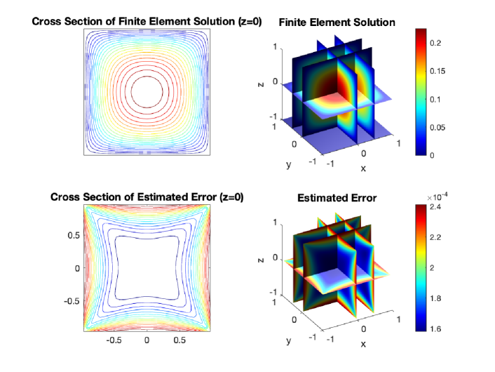
Figure 5. Solution and estimated energy error distribution for test problem 1.

Exploiting Galerkin orthogonality, the exact energy error can be estimated by comparing the energy of a reference solution with the energy of the computed finite element solution $\|u_{\rm ref}-u_{h}\|_{E}^{2}=\|u_{\rm ref}\|_{E}^{2}-\|u_{h}\|_{E}^{2}.$ Estimated errors that are computed using this strategy are presented in Table 1.

Table 1. Estimated energy errors for convex domain test problem.

		$\mathbb{Q}_{1}\qquad$		$\mathbb{Q}_{2}$
$n_{e}$	$h$	$\|u_{h}\|^{2}_{E}$	$\|u_{\rm ref}-u_{h}\|_{E}$	$n_{e}$	$\|u_{h}\|^{2}_{E}$	$\|u_{\rm ref}-u_{h}\|_{E}$
$8^{3}$	$0.2500$	$0.6233020$	$0.148627$	$4^{3}$	$0.6434550$	$0.044011$
$16^{3}$	$0.1250$	$0.6397600$	$0.075046$	$8^{3}$	$0.6452138$	$0.013348$
$32^{3}$	$0.0625$	$0.6439755$	$0.037636$	$16^{3}$	$0.6453773$	$0.003826$
$64^{3}$	$0.0313$	$0.6450372$	$0.018833$	$32^{3}$	$0.6453909$	$0.001029$
$128^{3}$	$0.0156$	$0.6453033$	$0.009416$	$64^{3}$	$0.6453919$	—

We observe that the $\mathbb{Q}_{1}$ energy errors are reducing by a factor of 2 with each grid refinement. This is consistent with the optimal $O(h)$ rate of convergence predicted theoretically in the case of a $H^{2}$-regular problem. The $\mathbb{Q}_{2}$ energy errors are reducing more rapidly with grid refinement. The observed rate is slightly less than $O(h^{2})$ which is the expected rate when solving a $H^{3}$-regular problem using triquadratic approximation.

Test problem 2 (Nonconvex domain).

A $\mathbb{Q}_{1}$ finite element solution to the Poisson problem (1)–(2) defined on the domain $D={[-1,1]^{3}\setminus[-1,0)\times[-1,0)\times[-1,1]}$ is shown in Fig. 6. In this computation the stair-shaped domain has been subdivided uniformly into $32^{3}-16^{2}\times 32$ elements. The dimension of the resulting linear algebra system is 27,489. The MATLAB R2021b sparse direct solver solves this system in about one fifth of a second. The error plot illustrates the edge singularity in the solution along the reentrant corner edge $(x=0,y=0,z)$.

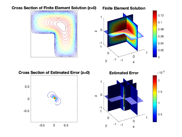
Figure 6. Solution and estimated energy error distribution for test problem 2.

Table 2. Estimated energy errors for the staircase domain test problem.

		$\mathbb{Q}_{1}\qquad$		$\qquad\mathbb{Q}_{2}$
$n_{e}$	$h$	$\|u_{h}\|^{2}_{E}$	$\|u_{ref}-u_{h}\|_{E}$	$n_{e}$	$\|u_{h}\|^{2}_{E}$	$\|u_{ref}-u_{h}\|_{E}$
$384$	$0.2500$	$0.2743216$	$0.149663$	$48$	$0.2933030$	$0.058461$
$3,072$	$0.1250$	$0.2905480$	$0.078566$	$384$	$0.2958987$	$0.028670$
$24,576$	$0.0625$	$0.2949834$	$0.041680$	$3,072$	$0.2964596$	$0.016157$
$196,608$	$0.0313$	$0.2962188$	$0.022402$	$24,576$	$0.2966318$	$0.009424$
$1,572,864$	$0.0156$	$0.2965759$	$0.012030$	$196,608$	$0.2967206$	—

Estimated errors for the second test problem are presented in Table 2. In this case we observe that the $\mathbb{Q}_{1}$ and $\mathbb{Q}_{2}$ energy errors are both reducing by a factor of less than 2 with each grid refinement. This is exactly what one would expect—the edge singularity limits the rate of convergence that is possible using uniform grids. The second notable feature is that the $\mathbb{Q}_{2}$ energy error is a factor of 2 smaller than the $\mathbb{Q}_{1}$ error for the same number of degrees of freedom (the results on the same horizontal line). This behaviour is also consistent with expectations; see Schwab [14].

Test problem 3 (borehole domain).

A $\mathbb{Q}_{1}$ finite element solution to the Poisson problem (1)–(2) defined on the cut domain $D={[-1,1]^{3}\setminus(-\epsilon,\epsilon)\times[0,1]\times(-\epsilon,\epsilon)}$ with $\epsilon=0.01$ is shown in Fig. 7.

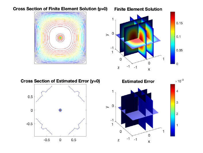
Figure 7. Solution and estimated energy error distribution for test problem 3.

In this computation the borehole domain has been subdivided into a tensor-product grid of $48\times 32\times 48$ elements with geometric stretching in the $x$ and $z$ direction so as to capture the geometry without using an excessive number of elements. The grid spacing increases from $h_{\min}=0.01=\epsilon$ within the hole to $h_{\max}=0.0625$ next to the boundary, so the maximum element aspect ratio (adjacent to the hole) is 6.25. The dimension of the resulting linear algebra system is 85,833 and the MATLAB R2021b sparse direct solver solves the system in about 6 seconds. As anticipated, the error in the approximation is concentrated in a small region in the neighbourhood of the borehole, making this a very challenging problem to solve efficiently.

4. Structure of the software package

IFISS is designed for the MATLAB coding environment. This means that the source code is readable, portable and easy to modify. All local calculations (quadrature in generating element matrices, application of essential boundary conditions, a posteriori error estimation) are vectorised over elements—thus the code runs efficiently on contemporary Intel processor architectures. IFISS3D has been developed for MATLAB (post 2016b) and tested with the current release (7.2) of Gnu Octave. The main directory is called diffusion3D and this needs to be added as a subdirectory of the main IFISS directory. The subdirectories of diffusion3D are organised as follows.

$\bullet$/grids/
This directory contains all the functions associated with domain discretisation. Three types of domain are included in the first release. Introducing a new domain type is straightforward. A new function needs to be included that saves nodal information (arrays xyz, bound3D) and (triquadratic) element information (mv, mbound3D) in an appropriately named datafile. This file will be subsequently read by an appropriate driver function associated with the specific PDE being solved.

$\bullet$/graphs/
This directory contains the functions associated with the visualisation of the computed solution (nodal data) and the estimated errors (element data). The tensor-product subdivision structure simplifies the code structure substantially—plotting can be efficiently done using the built-in slice functionality. Similarly, solution data defined on a one-dimensional incision into the domain of interest can be plotted using the function xyzsectionplot. An illustration is shown in Fig. 8.

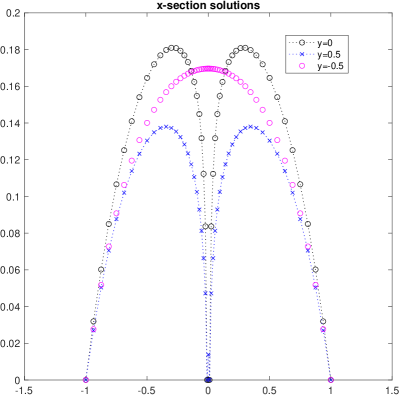
Figure 8. Incisions through the borehole test problem solution visualised in Fig. 7. The incisions show the solution in the $x$ direction in the plane $z=0$ for three different height values $y$.

$\bullet$/approximation/
This directory contains all the functions associated with setting up the discrete matrix system associated with the PDE of interest. The functions femq1_diff3D and femq2_diff3D set up the stiffness and mass matrices associated with the problems discussed in Section 3. Essential boundary conditions are imposed by a subsequent call to the function nonzerobc3D. Extending the functionality by combining components of IFISS with IFISS3D to cover (a) nonisotropic diffusion and (b) Stokes flow problems (using $\mathbb{Q}_{2}$–$\mathbb{Q}_{1}$ mixed approximation) is a straightforward exercise. Efficient approximation of the solution of the heat equation on a three-dimensional domain can also be done with ease: either using the adaptive time stepping functionality built into IFISS or using one of the ODE integrators built into MATLAB. The functions associated with a posteriori error estimation can be found in four separate subdirectories associated with the four options described in Section 2.

$\bullet$/solvers/
The MATLAB sparse direct solver ($\backslash$) has far from optimal complexity in a three-dimensional setting. This is explored in a case study in the next section. Algebraic multigrid (AMG) functionality is included in this directory to enable exploration of an optimal solution strategy. If one does not have access to an efficient AMG setup routine then the linear solver that is recommended when the dimension of the system exceeds $10^{5}$ is MINRES (Minimum Residual) iteration preconditioned by an incomplete Cholesky factorisation of the system matrix with zero fill-in.. This strategy is encoded in the it_solve3D function with a residual stopping tolerance of $10^{-10}$. Solving the system in Example 3 using this strategy gives a solution in 66 iterations. The associated CPU time is half a second. This is over 10 times faster on a 2018 MacBook than the corresponding backslash solve!

$\bullet$/test_problems/
This directory contains all the high-level driver functions such as diff3D_testproblem (the main driver). It also contains the functions associated with the problem data (right-hand side function and essential boundary specifications). The structure makes it straightforward to solve (1) together with nonzero boundary data $u=g_{D}$ on $\partial D$.

Help for IFISS is integrated into the MATLAB help facility. Typing helpme_diff3D gives information on solving a Poisson problem in three dimensions. Starting from the main IFISS directory, typing help diffusion3D/⟨subdirectory name⟩ gives a complete list of the files in that subdirectory. Using MATLAB, the function names are “clickable” to give additional information.

5. Case studies

Two important aspects of three-dimensional finite element approximation that can be investigated easily in IFISS3D are discussed in this section.

5.1. Effectivity of a posteriori error estimation strategies

The effectiveness of hierarchical error estimation is well established in a two-dimensional setting; see, for example, Elman et al. [9, Table 1.4]. The IFISS3D software offers a choice of 4 such error estimation strategies in conjunction with $\mathbb{Q}_{1}$ approximation. Computed error estimates obtained when solving the first test problem discussed in Section 3 are presented in Table 3. The four estimates are associated with the white nodes shown in Fig. 4. The estimated energy errors should be compared with the reference energy errors listed in Table 1.

Table 3. Computed error estimates $\eta_{\bullet}$ for the first test problem using four different hierarchical strategies.

$n_{e}$	$h$	$\eta_{\mathbb{Q}_{2}(h)}$	$\eta_{\mathbb{Q}^{r}_{2}(h)}$	$\eta_{\mathbb{Q}_{1}(h/2)}$	$\eta_{\mathbb{Q}^{r}_{1}(h/2)}$
$8^{3}$	$0.1250$	$0.150207$	$0.137906$	$0.129842$	$0.115359$
$16^{3}$	$0.0625$	$0.075177$	$0.069772$	$0.065255$	$0.058216$
$32^{3}$	$0.0313$	$0.037648$	$0.035050$	$0.032655$	$0.029215$
$64^{3}$	$0.0156$	$0.018837$	$0.017561$	$0.016326$	$0.014631$
$128^{3}$	$0.0078$	$0.009420$	$0.008789$	$0.008161$	$0.007321$

Table 4 lists the associated effectivity indices. The indices get closer to 1 as the mesh is refined when the $\mathbb{Q}_{2}(h)$ and $\mathbb{Q}^{r}_{2}(h)$ strategies are employed. On the other hand, the effectivity indices for the $\mathbb{Q}_{1}(h/2)$ and ${\mathbb{Q}^{r}_{1}(h/2)}$ strategies stagnate around $0.87$ and $0.77$ respectively. All four error estimates are correctly reducing by a factor of 2 with each grid refinement. In light of these results, the relatively cheap ${\mathbb{Q}^{r}_{2}(h)}$ is set to be the default option in IFISS3D. Extensive testing on other problems indicates that this estimator consistently underestimates the error by a small amount.

Table 4. Effectivity indices $\theta_{\bullet}\coloneqq\eta_{\bullet}/\|u_{ref}-u_{h}\|_{E}$ for test problem 1.

$n_{e}$	$\theta_{\mathbb{Q}_{2}(h)}$	$\theta_{\mathbb{Q}^{r}_{2}(h)}$	$\theta_{\mathbb{Q}_{1}(h/2)}$	$\theta_{\mathbb{Q}^{r}_{1}(h/2)}$
$8^{3}$	$\boldsymbol{1.0106}$	$\boldsymbol{0.9279}$	$\boldsymbol{0.8736}$	$\boldsymbol{0.7762}$
$16^{3}$	$\boldsymbol{1.0017}$	$\boldsymbol{0.9297}$	$\boldsymbol{0.8695}$	$\boldsymbol{0.7757}$
$32^{3}$	$\boldsymbol{1.0003}$	$\boldsymbol{0.9313}$	$\boldsymbol{0.8677}$	$\boldsymbol{0.7762}$
$64^{3}$	$\boldsymbol{1.0002}$	$\boldsymbol{0.9325}$	$\boldsymbol{0.8669}$	$\boldsymbol{0.7769}$

All the errors reported in Table 3 were computed after making a boundary element correction. This is a postprocessing step wherein the local problems associated with elements that have one or more boundary faces are modified so that the (zero) error on the boundary is enforced as an essential boundary condition. The motivation for making this correction is to recover the property of asymptotic exactness in special cases. The correction is, however, difficult to vectorise efficiently, raising the question as to whether it is worth including in a three-dimensional setting.

Computed effectivity indices for the special case of solving the Poisson problem

$$-\nabla^{2}u =f\quad\text{in }D=[-1,1]^{3}$$ (3)

$$u =0\quad\text{on }\partial D$$ (4)

with the right-hand side function $f$ chosen so that the exact solution is the triquadratic function

$$u(\boldsymbol{x}) =(1-x^{2})(1-y^{2})(1-z^{2}),$$ (5)

are presented in Table 5. The second and fourth columns are the results computed after making the boundary correction. The asymptotic exactness of the $\mathbb{Q}_{2}(h)$ strategy can be clearly seen. The third and fifth columns list the results that are computed when the boundary correction is not made. Comparing results with the second and fourth columns it is evident that the boundary correction reduces the estimated error and, more importantly, that the size of correction tends to zero in the limit $h\to 0$. The ${\mathbb{Q}^{r}_{2}(h)}$ strategy is not asymptotically exact so to speed up the computation the default setting in IFISS3D is to simply neglect the boundary correction. Thus, in the case of the finest grid in Table 5 (over 2 million elements) the $\eta^{*}_{\mathbb{Q}^{r}_{2}(h)}$ error estimate is computed in less than 9 seconds. This is significantly less than the time taken to compute the finite element solution itself (the it_solve3D linear system solve took over 23 seconds).

Table 5. Effectivity indices $\theta_{\bullet}\coloneqq\eta_{\bullet}/\|u_{ref}-u_{h}\|_{E}$ for the Poisson problem (3)–(5). The superscript $\theta^{*}_{\bullet}$ indicates that the boundary correction is omitted in the computation of $\eta_{\bullet}$.

$n_{e}$	$\theta_{\mathbb{Q}_{2}(h)}$	$\theta^{*}_{\mathbb{Q}_{2}(h)}$	$\theta_{\mathbb{Q}^{r}_{2}(h)}$	$\theta^{*}_{\mathbb{Q}^{r}_{2}(h)}$
$16^{3}$	$\boldsymbol{0.99944}$	$\boldsymbol{1.2914}$	$\boldsymbol{0.97044}$	$\boldsymbol{0.99647}$
$32^{3}$	$\boldsymbol{0.99990}$	$\boldsymbol{1.1508}$	$\boldsymbol{0.97087}$	$\boldsymbol{0.98289}$
$64^{3}$	$\boldsymbol{0.99998}$	$\boldsymbol{1.0771}$	$\boldsymbol{0.97110}$	$\boldsymbol{0.97686}$
$128^{3}$	$\boldsymbol{1.00000}$	$\boldsymbol{1.0390}$	$\boldsymbol{0.97123}$	$\boldsymbol{0.97405}$

5.2. Fast linear algebra

The solution of the (Galerkin) linear system is the computational bottleneck when solving a Poisson problem in three dimensions. To illustrate this point, a representative timing comparison of the distinct solution components when solving the first test problem using $\mathbb{Q}_{1}$ approximation with default settings is presented in Table 6. The system assembly includes the grid generation. The overall time is the elapsed time from start to finish and includes the time taken to visualise the solution and the associated error. What is immediately apparent is the fact that the system assembly times and the error estimation times scale approximately linearly with the number of elements (or equivalently, the dimension $n$ of the system matrix). The backslash solve times, in contrast, grow like the square of the number of elements on the most refined grids. The memory requirement for the sparse factors of the system matrix also increases at a much faster rate than $O(n)$.

Table 6. Representative component timings (in seconds) when solving test problem 1

$n_{e}$	assembly	solve ($\backslash$)	estimation	overall
$16^{3}$	$0.171$	$\boldsymbol{0.016}$	$0.617$	$\boldsymbol{1.10}$
$32^{3}$	$0.669$	$\boldsymbol{0.339}$	$1.481$	$\boldsymbol{4.81}$
$64^{3}$	$7.100$	$\boldsymbol{25.29}$	$11.49$	$\boldsymbol{58.1}$
$128^{3}$	$90.16$	$>\boldsymbol{10^{3}}$	$98.45$	$>\boldsymbol{10^{3}}$

The optimal $O(n)$ complexity of the overall solution algorithm can be recovered by solving the linear system using a short-term Krylov subspace iteration such as MINRES in combination with an algebraic multigrid (AMG) preconditioning strategy; see [9, sec. 2.5.3]. The set up phase of AMG is a recursive procedure: heuristics associated with algebraic relations (“strength of connections”) between the unknowns are used to generate a sequence of progressively coarser representations $A_{\ell}$, $\ell=1,2,\ldots,L$ of the Galerkin system matrix $A\coloneqq A_{1}$. The solution (preconditioning) phase approximates the action on the inverse of $A$ on a vector by cycling through the associated grid sequence. At each level, a fixed-point iteration (typically point Gauss-Seidel) is applied to “smooth” the residual error that is generated by interpolation or restriction of the error vector generated at the previous level. If coarsening is sufficiently rapid then the work associated with the preconditioning step will be proportional to the number of unknowns.

The algorithmic complexity of any AMG coarsening strategy can be characterised by a few parameters. First, the grid complexity is defined as

$$c_{G}\coloneqq\frac{1}{n_{1}}\sum_{\ell=1}^{L}n_{\ell},$$

where $n_{\ell}$ is the dimension of the coarse grid matrix $A_{\ell}$ at level $\ell$. Starting from a uniform grid of $\mathbb{Q}_{1}$ elements, if full coarsening (in each spatial direction) is done at each level then $n_{\ell}$ reduces by a factor of $8$ at each level, in which case we obtain $c_{G}\approx{8}/{7}$. A value of $c_{G}$ higher than this suggests that coarsening has not been done isotropically. The operator complexity is typically defined by

$$c_{A}\coloneqq\frac{1}{{\rm nnz}(A_{1})}\sum_{\ell=1}^{L}{\rm nnz}(A_{\ell}),$$

where ${\rm nnz}(A)$ is the number of nonzeros in the matrix. This parameter provides information about the associated storage requirements for the coarse grid matrices generated. If uniform coarsening is done and the coarse grid matrices correspond to the usual finite element discretisation on those grids then we would expect $c_{A}\approx c_{G}$. In practice however, the coarse grid matrices become progressively denser, with larger stencil sizes, as the level number increases. If the matrices become too dense then this may cause an issue with the computational cost of applying the chosen smoother. To quantify this, the average stencil size

$$c_{S}:=\frac{1}{L}\sum_{\ell=1}^{L}\frac{{\rm nnz}(A_{\ell})}{n_{\ell}},$$

should be compared with the average stencil size at the finest level, that is,

$$c_{1}\coloneqq\frac{{\rm nnz}(A_{1})}{n_{1}}.$$

An implementation of the coarsening strategy developed by Ruge and Stüben [13] is included in the IFISS software. The corresponding IFISS3D function amg_grids_setup3D can be edited in order to explore algorithmic options or change the default threshold parameters. The MATLAB implementation of the coarsening algorithm is far from optimal however. There is a marked deterioration in performance when solving problems on fine grids that is evident even when solving Poisson problems in two dimensions. To address this issue an interface to the efficient Fortran 95 implementation [10] of the same coarsening algorithm is included in IFISS3D.

Table 7. AMG grid complexity data and representative linear solver timings for test problem 1.

	$\mathbb{Q}_{1}$				$\mathbb{Q}_{2}$
$n_{e}$	$16^{3}$	$32^{3}$	$64^{3}$	$128^{3}$	$16^{3}$	$32^{3}$	$64^{3}$
$n_{1}$	4,913	35,937	274,625	2,146,689	35,937	274,625	2,146,689
$c_{1}$	16.49	21.14	23.90	25.41	47.06	54.96	59.33
$L$	7	11	16	14	11	14	16
$c_{G}$	1.24	1.32	1.37	1.39	1.27	1.32	1.32
$c_{A}$	1.58	1.77	1.88	1.93	1.61	1.70	1.76
$c_{S}$	22.9	39.2	62.8	97.6	65.59	106.1	138.8
setup∗ time	0.01	0.07	0.58	5.12	0.15	1.22	11.49
total time	0.02	0.16	1.49	13.07	0.42	3.48	33.60

AMG complexities and timings obtained when solving test problem 1 are presented in Table 7. The total times reported for the $\mathbb{Q}_{1}$ approximation should be compared with the corresponding backslash solve timings recorded in Table 6. The setup times were recorded using the interface to the HSL_MI20 code and scale close to linearly with the problem dimension. This behaviour is consistent with the results that were reported for the same problem and discretisation by Boyle et al. [4, Ex. 4.5.1]. Looking at the AMG grid data in Table 7, we note that the grid complexity is under control and stays close to the optimal value using either of the two approximation strategies. The operator complexity results are also encouraging—increasing slowly as the dimension of the problem is increased. The growth in the average stencil size is not unexpected. The value of $c_{S}$ is within a factor of 3 of $c_{1}$ when using $\mathbb{Q}_{2}$ approximation on the finest grid. The difference between the highlighted total time and the associated setup time is the time taken by preconditioned MINRES to reach the residual stopping tolerance of $10^{-10}$ with the default smoothing parameters (that is, two pre- and post-smoothing sweeps using point Gauss-Seidel).

The (Ruge–Stüben) AMG coarsening strategy is designed to be effective even in cases where the discretised problem has strong anisotropy in the grid spacing. This is validated by the encouraging timing results for the borehole problem that are presented in Table 8. Here, $l$ denotes the level of refinement of the finite element mesh.

Table 8. AMG grid complexity data and representative linear solver timings for test problem 3.

	$\mathbb{Q}_{1}$
	$l=2$	$l=3$	$l=4$	$l=5$
$n_{1}$	85,833	365,625	1,264,329	3,888,153
$c_{1}$	22.41	24.15	25.08	25.61
$L$	15	16	18	18
setup∗ time	0.44	2.42	8.48	26.47
total time	1.08	6.89	24.05	79.20

6. Summary and future developments

The IFISS3D toolbox extends the capabilities of IFISS [15] to facilitate the numerical solution of elliptic PDEs on three-dimensional spatial domains that can be partitioned into hexahedra. In particular, it allows users to investigate the convergence properties of trilinear ($\mathbb{Q}_{1}$) and triquadratic ($\mathbb{Q}_{2}$) finite element approximation for test problems whose solutions have varying levels of spatial regularity and the performance of a range of iterative solution algorithms for the associated discrete systems, including an optimal AMG solver. For $\mathbb{Q}_{1}$ approximation, the effectivity of four distinct state-of-the-art hierarchical error estimation schemes can also be explored. The IFISS3D software is structured in such a way that, when integrated into the existing IFISS software, users can easily solve a range of other PDE problems, including time-dependent ones, using $\mathbb{Q}_{1}$ and $\mathbb{Q}_{2}$ elements on three-dimensional spatial domains. IFISS together with IFISS3D is intended to be useful as a teaching tool, and can be used to produce matrices of arbitrarily large dimension for testing linear algebra algorithms. Future developments of IFISS3D will be documented on GitHub.

References

- [1] R. B. Bank and R. K. Smith, A posteriori error estimates based on hierarchical bases, SIAM J. Numer. Anal., 30 (1993), pp. 921–935. https://www.jstor.org/stable/2158183.
- [2] A. Bespalov, L. Rocchi, and D. J. Silvester, T-IFISS: a toolbox for adaptive FEM computation, Comput. Math. Appl., 81 (2021), pp. 373–390. https://doi.org/10.1016/j.camwa.2020.03.005.
- [3] M. Blatt, A. Burchardt, A. Dedner, et al., The Distributed and Unified Numerics Environment, version 2.4, Arch. Num. Soft., 4 (2016), pp. 13–29.
- [4] J. Boyle, M. Mihajlović, and J. Scott, HSL_MI20: an efficient AMG preconditioner for finite element problems in 3D, Int. J. Numer. Meth. Engng., 82 (2010), pp. 64–98.
- [5] A. J. Crowder, G. Papanikos, and C. E. Powell, ML-SGFEM (Multilevel Stochastic Galerkin Finite Element Method) Software, version 1.0, 2022. https://github.com/ceapowell/ML_SGFEM.
- [6] A. J. Crowder, C. E. Powell, and A. Bespalov, Efficient adaptive multilevel stochastic Galerkin approximation using implicit a posteriori error estimation, SIAM J. Sci. Comput., 41 (2019), pp. A1681–A1705.
- [7] H. Elman, A. Ramage, and D. Silvester, Algorithm 866: IFISS, a Matlab toolbox for modelling incompressible flow, ACM Trans. Math. Softw., 33 (2007), pp. 2–14. http://dx.doi.org/10.1145/1236463.1236469.
- [8] , IFISS: A computational laboratory for investigating incompressible flow problems, SIAM Review, 56 (2014), pp. 261–273. http://dx.doi.org/10.1137/120891393.
- [9] H. Elman, D. Silvester, and A. Wathen, Finite Elements and Fast Iterative Solvers: with Applications in Incompressible Fluid Dynamics, Oxford University Press, Oxford, UK, 2014. Second Edition.
- [10] HSL mathematical software library, 2015. https://www.hsl.rl.ac.uk/catalogue/hsl_mi20.html.
- [11] A. Logg, K.-A. Mardal, G. N. Wells, et al., Automated Solution of Differential Equations by the Finite Element Method, Springer, 2012. https://fenicsproject.org/.
- [12] G. Papanikos, C. E. Powell, and D. Silvester, Incompressible Flow and Iterative Solver 3D Software (IFISS3D), version 1.0, 2022. https://github.com/mcbssds/IFISS3D.
- [13] J. Ruge and K. Stüben, Algebraic multigrid, in Multigrid Methods, S. F. McCormick, ed., vol. 3 of Frontiers in Applied Mathematics, SIAM, Philadelphia, PA, 1987, pp. 73–130.
- [14] C. Schwab, p- and hp- Finite Element Methods: Theory and Applications in Solid and Fluid Mechanics, Oxford University Press, Oxford, UK, 1998.
- [15] D. Silvester, H. Elman, and A. Ramage, Incompressible Flow and Iterative Solver Software (IFISS), version 3.6, February 2019. http://www.manchester.ac.uk/ifiss/.
- [16] An information service for mathematical software, 2022. https://swmath.org/software/4398.