Tangential Tensor Fields on Deformable Surfaces – How to Derive Consistent $L^{2}$-Gradient Flows

Abstract

We consider gradient flows of surface energies which depend on the surface by a parameterization and on a tangential tensor field. The flow allows for dissipation by evolving the parameterization and the tensor field simultaneously. This requires to chose a notion of independence. We introduce different gauges of surface independence and show their consequences for the evolution. In order to guarantee a decrease in energy the gauge of surface independence and the time derivative have to be chosen consistently. We demonstrate the results for a surface Frank-Oseen energy.

1 Introduction

Gradient flows are evolutionary systems which decrease an energy by a dissipation mechanism. Such systems are common in physics and are widely explored in mathematics. In this work, we consider classical Hilbert spaces, the $L^{2}$-norm as dissipation mechanism and surface energies $\mathfrak{U}[\boldsymbol{X},\boldsymbol{q}[\boldsymbol{X}]]$ depending on a surface $\mathcal{S}$ by a parameterization $\boldsymbol{X}$ and on a tangential n-tensor field $\boldsymbol{q}[\boldsymbol{X}]\in\tensor{\operatorname{T}\!}{{}^{n}}\mathcal{S}$, see section 2 for definitions. The tangential n-tensor field $\boldsymbol{q}[\boldsymbol{X}]$ is defined with respect to its frame, which introduces a dependency on the parameterization $\boldsymbol{X}$. $L^{2}$-gradient flows of such surface energies, which allow for dissipation by evolving $\boldsymbol{X}$ and $\boldsymbol{q}[\boldsymbol{X}]$ simultaneously, read

$$\left(\boldsymbol{V}[\boldsymbol{X}],\mathfrak{D_{t}}\boldsymbol{q}[\boldsymbol{X}]\right)=-\lambda\nabla_{\operatorname{L}^{\!2}}\mathfrak{U},$$ (1)

where $\boldsymbol{V}$ denotes the velocity of the surface $\mathcal{S}$ and $\mathfrak{D_{t}}\boldsymbol{q}[\boldsymbol{X}]$ denotes an observer-invariant instantaneous time derivative of the n-tensor field $\boldsymbol{q}[\boldsymbol{X}]$, see Nitschke_2022 . To give the $L^{2}$-gradient on the right hand side of (1) a mathematical meaning is the content of this paper. The delicate issue is the requirement of mutual independence of $\boldsymbol{X}$ and $\boldsymbol{q}[\boldsymbol{X}]$. But what does this actually mean? When is a tensor field independent of its underlying spatial domain? How strong does such a independence has to be for the purpose of variation? We investigate these issues for variations of first kind and reveal consequences for such $\operatorname{L}^{\!2}$-gradient flows, e. g., the requirement to chose the notion of independence consistent with the time derivative. Furthermore we provide physical cues to chose an appropriate notion of independence or a related time derivative. While this choice might be intuitive for elastic surfaces Gurtin_ARMA_1975 ; steigmann2007thin ; Yavarietal_JNS_2016 ; sadik2016shells ; Lewicka_book_2022 ; pezzulla2022geometrically and fluidic surfaces scriven1960dynamics ; Arroyoetal_PRE_2009 ; Reutheretal_MMS_2015 ; Kobaetal_QAM_2017 ; jankuhn2018 ; Miura_QAM_2018 ; Reutheretal_MMS_2018 ; Kobaetal_QAM_2018 ; guven2018geometry ; torres2019modelling ; reuther2020numerical , this changes for viscoelastic surfaces Snoeijer_PRSA_2020 ; deKinkelder_JCP_2021 and surface liquid crystals Reuteretal_PRSA_2019_Preprint ; Reuteretal_PRSA_2020 . Crucial examples where the last two are of relevance are biological surfaces, e. g., the actomyosin cortex which drives cell surface deformations or on a larger scale epithelia tissue which deforms during morphogenesis. Existing models for such applications are still at its infancy Mietke_PNAS_2019 ; deKinkelder_JCP_2021 ; Maroudas-Sacks_NP_2021 ; Hoffmann_SA_2022 ; SalbreuxJuelicherProstCallan-Jones__2022 ; Morris_2022 . However, they all have in common to chose the notion of independence and the time derivative in an adhoc fashion. As these systems are by definition out of equilibrium, the dynamics matters. We will demonstrate the dependency of the dynamics on the notion of independence. Any quantitative study of such systems therefore requires to deal with these issues.

The paper is structured as follows: In section 2 we introduce linear deformed surfaces and some necessary mathematical tools, which cover independence of coordinates and leave the surface as a degree of freedom. We implement in section 3 deformation derivatives for tensor fields, which leads us to the concept of the gauge of surface independence. Treating scalar fields in subsection 3.1 is merely a warm-up exercise to make ourselves familiar with the concept of the deformation derivative and surface independence. However, this changes for tangential vector- and tensor- fields, which we approach in subsection 3.2 and 3.3. For instance, we see that the variation of an energy depending on the contravariant proxy of a tensor field, which is assumed to be independent of the surface, leads to a different result then the same variation for the same energy but with a covariant proxy assumed to be independent. It cannot be due to the co- or contravariant frame, since the calculus is invariant w. r. t. frames, resp. musical isomorphisms. So the reason has to lie in the assumption of independence as a consequence. We elaborate this discrepancy for tangential vector fields in subsection 3.2, introduce four different gauges of surface independence and relate them mutually. That includes some useful identities for calculating surface variations. We also show the influence on the $\operatorname{L}^{\!2}$-gradient out of an equilibrium state, which in turn does have an impact on the $\operatorname{L}^{\!2}$-gradient flow. This can be read from the energy rate of the surface energy. In section 3.3 we extend our results to $2$-tensor fields, thus providing the reader with a roadmap for further extensions to $n$-tensor fields, since the proceeding is almost always the same. We make the differences between the various gauges of surface independence visible using an example in section 4, where the $\operatorname{L}^{\!2}$-gradient flow for the surface Frank-Oseen energy is solved numerically under all gauges of surface independence. Finally we draw conclusions in section 5.

2 Notations and Mathematical Preliminaries

2.1 Surfaces and Linear Deformations

For our purpose a surface is a 2-dimensional Riemannian manifold $(\mathcal{S},\boldsymbol{g})$ smoothly embededed in the 3-dimensional Euclidean space $\mathbb{R}^{3}$ by a smooth parameterization

$$\boldsymbol{X}=\begin{bmatrix}X^{1}\\ X^{2}\\ X^{3}\end{bmatrix}:\quad\mathcal{U}\rightarrow\mathbb{R}^{3}:\quad(y^{1},y^{2})\mapsto\boldsymbol{X}(y^{1},y^{2})\in\mathcal{S}\,\text{,}$$ (2)

where $\mathcal{U}\subset\mathbb{R}^{2}$. For simplicity we assume that $\boldsymbol{X}(\mathcal{U})=\mathcal{S}$ can be achieved by a single parameterization $\boldsymbol{X}$. The results can be extended to the more general case considering subsets providing an open covering of $\mathcal{S}$. As $\boldsymbol{X}$ determines $\mathcal{S}$, the dependency of a surface can be described by the dependency of its parameterization. This has advantageous as $\boldsymbol{X}$ is defined in the embedding space, which bears vector space structure and allows to work with vector calculus. For simplicity we will also avoid boundaries. If boundary terms become necessary they are inserted at the appropriated places.

Field quantities are always given w. r. t. the local parameter space $\mathcal{U}$. Therefore, we describe a vector field $\boldsymbol{W}\in\tensor{\operatorname{T}\!}{}\mathbb{R}^{3}|_{\mathcal{S}}$ by

$$\boldsymbol{W}=\begin{bmatrix}W^{1}\\ W^{2}\\ W^{3}\end{bmatrix}:\quad\mathcal{U}\rightarrow\mathbb{R}^{3}:\quad(y^{1},y^{2})\mapsto\boldsymbol{W}(y^{1},y^{2})\in\tensor{\operatorname{T}\!}{}_{\boldsymbol{X}(y^{1},y^{2})}\mathbb{R}^{3}\equiv\mathbb{R}^{3}\,\text{,}$$

which fulfill the restriction to $\mathcal{S}$ by default. Comparing this with (2), we see that $\boldsymbol{X}+\varepsilon\boldsymbol{W}$, with $\varepsilon>0$, provides a parameterization for another surface $\mathcal{S}_{\varepsilon\boldsymbol{W}}$. Considering $\varepsilon$ sufficiently small and the scalar field $\left\|\boldsymbol{W}\right\|_{\tensor{\operatorname{T}\!}{}\mathbb{R}^{3}|_{\mathcal{S}}}$ to be finite locally w. r. t. $\mathcal{U}$, the surface $\mathcal{S}_{\varepsilon\boldsymbol{W}}$ is a finite deformation of the surface $\mathcal{S}$ in direction of $\boldsymbol{W}\in\tensor{\operatorname{T}\!}{}\mathbb{R}^{3}|_{\mathcal{S}}$, see figure 1. As $\boldsymbol{W}$ is only given on the undeformed surface $\mathcal{S}$ and can be defined independently of the parameterization $\boldsymbol{X}$ it does not bear the functional argument $\boldsymbol{X}$, i. e., $\boldsymbol{W}=\boldsymbol{W}[\boldsymbol{X}]$.

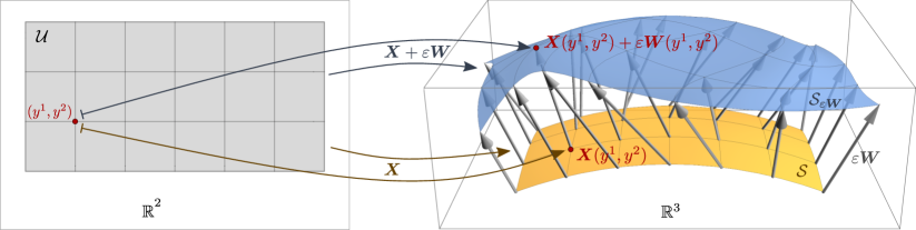
Figure 1: Schematic of parameterization and deformation: $\mathcal{U}=\{(y^{1},y^{2})\}\subset\mathbb{R}^{2}$ is the domain (left) of the parameterization $\boldsymbol{X}$, resp. $\boldsymbol{X}+\varepsilon\boldsymbol{W}$, which maps to the surface $\mathcal{S}\subset\mathbb{R}^{3}$ (lower right), resp. $\mathcal{S}_{\varepsilon\boldsymbol{W}}\subset\mathbb{R}^{3}$ (upper right). The surface $\mathcal{S}$ is linear deformed by $\varepsilon>0$ in direction of the field $\boldsymbol{W}\in\tensor{\operatorname{T}\!}{}\mathbb{R}^{3}|_{\mathcal{S}}$.

Note that we could also consider higher order deformation $\boldsymbol{X}+\varepsilon\boldsymbol{W}+\mathcal{O}(\varepsilon^{2})$. However, for the main results of the paper linear deformations are sufficient.

2.2 Notations

Lowercase Latin indices $\{i,j,k,\ldots\}$ belong to the coordinates $y^{1}$ and $y^{2}$ defined in the domain $\mathcal{U}\subset\mathbb{R}^{2}$ of parameterization $\boldsymbol{X}$. Uppercase indices $\{I,J,K,\ldots\}$ belong to Cartesian $\mathbb{R}^{3}$-coordinates. Moreover, Einstein summation convention is assumed throughout this paper. For instance, the covariant proxy components of the metric tensor are writeable by $g_{ij}[\boldsymbol{X}]=\delta_{IJ}(\partial_{i}X^{I})(\partial_{j}X^{J})$, where the short notation $\partial_{i}:=\frac{\partial}{\partial y^{i}}$ is in use. Arguments in square brackets indicate total functional dependencies. This also includes derivatives of the arguments. Moreover, we put indices in front of the square brackets for a better readability, e. g., we write $g_{ij}[\boldsymbol{X}]$ instead of $g[\boldsymbol{X}]_{ij}$ or $[\boldsymbol{g}[\boldsymbol{X}]]_{ij}$. We respect the order of indices in proxy notations except for symmetries in them, e. g., $\delta^{I}_{J}$ is allowed to be written, since $\tensor{\delta}{{}^{I}_{J}}=\tensor{\delta}{{}_{J}^{I}}$ is true.

We write $\boldsymbol{q}\in\tensor{\operatorname{T}\!}{{}^{n}}\mathcal{S}$ for short to state that $\boldsymbol{q}$ is a tangential $n$-tensor field, i. e., it holds $\boldsymbol{q}:\mathcal{U}\rightarrow\tensor*{\operatorname{T}\!}{{}^{n}_{\boldsymbol{X}(\mathcal{U})}}\mathcal{S}$. Same applies for $\boldsymbol{Q}\in\tensor{\operatorname{T}\!}{{}^{n}}\mathbb{R}^{3}|_{\mathcal{S}}$ to state $\boldsymbol{Q}:\mathcal{U}\rightarrow\tensor*{\operatorname{T}\!}{{}^{n}_{\boldsymbol{X}(\mathcal{U})}}\mathbb{R}^{3}$. Note that $\tensor{\operatorname{T}\!}{{}^{n}}\mathcal{S}$ is a linear subbundle of $\tensor{\operatorname{T}\!}{{}^{n}}\mathbb{R}^{3}|_{\mathcal{S}}$, i. e., it holds $\tensor*{\operatorname{T}\!}{{}^{n}_{\boldsymbol{X}(y^{1},y^{2})}}\mathcal{S}\leq\tensor*{\operatorname{T}\!}{{}^{n}_{\boldsymbol{X}(y^{1},y^{2})}}\mathbb{R}^{3}$ for all $(y^{1},y^{2})\in\mathcal{U}$, where the equality is only true for $n=0$. For $n=1$ we omit the order index, i. e., $\tensor{\operatorname{T}\!}{}:=\tensor{\operatorname{T}\!}{{}^{1}}$. If the exact type of tensor order is not important due to isomorphisms and operator invariance, then we write the order index superior, i. e., the tensor has fully contravariant order.

Bold symbols for tangential $n$-tensor fields, with $n>0$, consider the field with frame, in our case the frame from the embedding by $\boldsymbol{X}$. For instance, we write $\boldsymbol{q}=q^{i}\partial_{i}\boldsymbol{X}\in\tensor{\operatorname{T}\!}{}\mathcal{S}$ with frame $\{\partial_{i}\boldsymbol{X}\}$ and contravariant proxy field $(q^{1},q^{2})\in(\tensor{\operatorname{T}\!}{{}^{0}}\mathcal{S})^{2}$. However, scalar fields ($n=0$) are not written in bold symbols. This affects also components of tensor proxies like $q^{i}\in\tensor{\operatorname{T}\!}{{}^{0}}\mathcal{S}$.

Occasionally, we use a Cartesian frame $\{\boldsymbol{e}_{I}\}$ or a so-called thin film frame $\{\partial_{1}\boldsymbol{X},\partial_{2}\boldsymbol{X},\boldsymbol{\nu}[\boldsymbol{X}]\}$ restricted to the surface $\mathcal{S}$, with normal field $\boldsymbol{\nu}[\boldsymbol{X}]\bot\tensor{\operatorname{T}\!}{}\mathcal{S}$. The principle of covariance for the choice of coordinates ensures that every frame, according to its coordinates, is equivalent, as long as we obey a calculus, which preserves this principle. For instance the Ricci-calculus Schouten1954 or the use of covariant operators are sufficient for this.

2.3 Inner Products

For inner products we use angle brackets and mark them by their domain, e. g., it is $\left\langle\boldsymbol{q},\boldsymbol{r}\right\rangle_{\tensor{\operatorname{T}\!}{}\mathcal{S}}:=g_{ij}[\boldsymbol{X}]q^{i}r^{j}$ for $\boldsymbol{r},\boldsymbol{q}\in\tensor{\operatorname{T}\!}{}\mathcal{S}$ or $\left\langle\boldsymbol{Q},\boldsymbol{R}\right\rangle_{\tensor{\operatorname{T}\!}{}\mathbb{R}^{3}|_{\mathcal{S}}}:=\delta_{IJ}Q^{I}R^{J}$ for $\boldsymbol{Q},\boldsymbol{R}\in\tensor{\operatorname{T}\!}{}\mathbb{R}^{3}|_{\mathcal{S}}$. Since the metric tensor $\boldsymbol{g}$ is derived from the parameterization $\boldsymbol{X}$, and therefore gives an isometric embedding by definition, the local inner products $\left\langle\cdot,\cdot\right\rangle_{\tensor{\operatorname{T}\!}{{}^{n}}\mathcal{S}}$ and $\left\langle\cdot,\cdot\right\rangle_{\tensor{\operatorname{T}\!}{{}^{n}}\mathbb{R}^{3}|_{\mathcal{S}}}$ are equal on the subbundle $\tensor{\operatorname{T}\!}{{}^{n}}\mathcal{S}\leq\tensor{\operatorname{T}\!}{{}^{n}}\mathbb{R}^{3}|_{\mathcal{S}}$. For instance, the example above reveals $\left\langle\boldsymbol{q},\boldsymbol{r}\right\rangle_{\tensor{\operatorname{T}\!}{}\mathcal{S}}=\left\langle\boldsymbol{q},\boldsymbol{r}\right\rangle_{\tensor{\operatorname{T}\!}{}\mathbb{R}^{3}|_{\mathcal{S}}}$. The global inner product is a $\operatorname{L}^{\!2}$-product derived from the local one, i. e., we define

$$\left\langle\boldsymbol{Q},\boldsymbol{R}\right\rangle_{\operatorname{L}^{\!2}(\mathcal{T})} :=\int_{\mathcal{S}}\left\langle\boldsymbol{Q},\boldsymbol{R}\right\rangle_{\mathcal{T}}\mu[\boldsymbol{X}]=\int_{\mathcal{U}}\left\langle\boldsymbol{Q},\boldsymbol{R}\right\rangle_{\mathcal{T}}\sqrt{|\boldsymbol{g}[\boldsymbol{X}]|}dy^{1}\!\!\wedge\!dy^{2}$$

for $\mathcal{T}=\tensor{\operatorname{T}\!}{{}^{n}}\mathcal{S}$, resp.  $=\tensor{\operatorname{T}\!}{{}^{n}}\mathbb{R}^{3}|_{\mathcal{S}}$, and $\boldsymbol{Q},\boldsymbol{R}\in\tensor{\operatorname{T}\!}{{}^{n}}\mathcal{S}$, resp.  $\in\tensor{\operatorname{T}\!}{{}^{n}}\mathbb{R}^{3}|_{\mathcal{S}}$, where $|\boldsymbol{g}[\boldsymbol{X}]|$ is the determinant of the metric proxy $\{g_{ij}[\boldsymbol{X}]\}$ and $\mu[\boldsymbol{X}]$ the surface area form, which is in fact the 2-dimensional volume form, a differential 2-form. All norms are derived from their associated inner products, i. e., $\|\cdot\|_{\mathcal{T}}^{2}:=\left\langle\cdot,\cdot\right\rangle_{\mathcal{T}}$ for $\mathcal{T}\in\{\tensor{\operatorname{T}\!}{{}^{n}}\mathcal{S},\tensor{\operatorname{T}\!}{{}^{n}}\mathbb{R}^{3}|_{\mathcal{S}},\operatorname{L}^{\!2}(\tensor{\operatorname{T}\!}{{}^{n}}\mathcal{S}),\operatorname{L}^{\!2}(\tensor{\operatorname{T}\!}{{}^{n}}\mathbb{R}^{3}|_{\mathcal{S}})\}$.

2.4 Geometric Quantities

The covariant proxy of the metric tensor $\boldsymbol{g}$, also known as first fundamental form, is given by $g_{ij}[\boldsymbol{X}]=\left\langle\partial_{i}\boldsymbol{X},\partial_{j}\boldsymbol{X}\right\rangle_{\tensor{\operatorname{T}\!}{}\mathcal{S}}\in\tensor{\operatorname{T}\!}{{}^{0}}\mathcal{S}$. The normal field $\boldsymbol{\nu}[\boldsymbol{X}]\in\tensor{\operatorname{T}\!}{}\mathbb{R}^{3}|_{\mathcal{S}}$ can be calculated by

$$\sqrt{|\boldsymbol{g}[\boldsymbol{X}]|}\boldsymbol{\nu}[\boldsymbol{X}] =\partial_{1}\boldsymbol{X}\times\partial_{2}\boldsymbol{X}=\tensor{\epsilon}{{}^{I}_{JK}}\partial_{1}X^{J}\partial_{2}X^{K}\boldsymbol{e}_{I}$$

up to an orientation determining sign, where $\{\tensor{\epsilon}{{}^{I}_{JK}}\}$ are Levi-Civita symbols. The index position w. r. t. Cartesian space is only given for reasons of consistency with Einstein summation, though it does not change the values. However, this detail matters on tangential calculus. With Levi-Civita symbols $\{\epsilon_{ij}\}$, the covariant proxy field components of the surface Levi-Civita tensor $\boldsymbol{E}[\boldsymbol{X}]\in\tensor{\operatorname{T}\!}{{}^{2}}\mathcal{S}$ are given by $E_{ij}[\boldsymbol{X}]:=\sqrt{|\boldsymbol{g}[\boldsymbol{X}]|}\epsilon_{ij}$. As a bilinear map $\tensor{\operatorname{T}\!}{}\mathcal{S}\times\tensor{\operatorname{T}\!}{}\mathcal{S}\rightarrow\mathbb{R}$ this tensor field equals the differential 2-form $\mu[\boldsymbol{X}]$, or as a linear map $\tensor{\operatorname{T}\!}{{}_{1}}\mathcal{S}\rightarrow\tensor{\operatorname{T}\!}{{}_{1}}\mathcal{S}$ of differential 1-forms the Hodge-star operator. The relation between the Levi-Civita tensor field and $\mathbb{R}^{3}$-cross product is $\boldsymbol{q}\times\boldsymbol{r}=(\boldsymbol{q}\boldsymbol{E}[\boldsymbol{X}]\boldsymbol{r})\boldsymbol{\nu}[\boldsymbol{X}]$ for all $\boldsymbol{q},\boldsymbol{r}\in\tensor{\operatorname{T}\!}{}\mathcal{S}$.

The covariant proxy components of the second fundamental form are given by

$$I\!I_{ij}[\boldsymbol{X}] :=\left\langle\partial_{i}\partial_{j}\boldsymbol{X},\boldsymbol{\nu}[\boldsymbol{X}]\right\rangle_{\tensor{\operatorname{T}\!}{}\mathbb{R}^{3}|_{\mathcal{S}}}=-\left\langle\partial_{i}\boldsymbol{X},\partial_{j}\boldsymbol{\nu}[\boldsymbol{X}]\right\rangle_{\tensor{\operatorname{T}\!}{}\mathcal{S}}\,\text{.}$$ (3)

The associated 2-tensor field $\boldsymbol{I\!I}[\boldsymbol{X}]\in\tensor{\operatorname{T}\!}{{}^{2}}\mathcal{S}$ is symmetric and as a linear map $\tensor{\operatorname{T}\!}{}\mathcal{S}\rightarrow\tensor{\operatorname{T}\!}{}\mathcal{S}$ also known as shape-operator. We use these terminologies equivalently, since they are up to musical isomorphisms. Two scalar quantities can be derived from the second fundamental form. They are the mean and the Gaussian curvature $\mathcal{H}[\boldsymbol{X}],\mathcal{K}[\boldsymbol{X}\in\tensor{\operatorname{T}\!}{{}^{0}}\mathcal{S}$ defined by

$$\mathcal{H}[\boldsymbol{X}] :=\operatorname{Tr}\boldsymbol{I\!I}[\boldsymbol{X}]=I\!I^{i}_{i}[\boldsymbol{X}]\,\text{,}\quad\quad\mathcal{K}[\boldsymbol{X}]:=|\{I\!I^{i}_{j}\}|=\frac{|\{I\!I_{ij}\}|}{|\boldsymbol{g}|}\,\text{.}$$

2.5 Tangetial Projection

Since $\tensor{\operatorname{T}\!}{{}^{n}}\mathcal{S}$ is a subbundle of $\tensor{\operatorname{T}\!}{{}^{n}}\mathbb{R}^{3}|_{\mathcal{S}}$, an orthogonal projection $\operatorname{\Pi}_{\tensor{\operatorname{T}\!}{{}^{n}}\mathcal{S}}:\tensor{\operatorname{T}\!}{{}^{n}}\mathbb{R}^{3}|_{\mathcal{S}}\rightarrow\tensor{\operatorname{T}\!}{{}^{n}}\mathcal{S}$ can be uniquely defined. It can be described by

$$\operatorname{\Pi}_{\tensor{\operatorname{T}\!}{{}^{n}}\mathcal{S}}\boldsymbol{Q} =Q^{J_{1}\ldots J_{n}}\left(\prod_{\alpha=1}^{n}(\delta_{J_{\alpha}}^{I_{\alpha}}-\nu^{I_{\alpha}}[\boldsymbol{X}]\nu_{J_{\alpha}}[\boldsymbol{X}])\right)\bigotimes_{\alpha=1}^{n}\boldsymbol{e}_{I_{\alpha}}$$

$$=\left\langle\boldsymbol{Q},\bigotimes_{\alpha=1}^{n}\partial_{i_{\alpha}}\boldsymbol{X}\right\rangle_{\tensor{\operatorname{T}\!}{{}^{n}}\mathbb{R}^{3}|_{\mathcal{S}}}\left(\prod_{\alpha=1}^{n}g^{i_{\alpha}j_{\alpha}}[\boldsymbol{X}]\right)\bigotimes_{\alpha=1}^{n}\partial_{j_{\alpha}}\boldsymbol{X}$$

for all $\boldsymbol{Q}\in\tensor{\operatorname{T}\!}{{}^{n}}\mathbb{R}^{3}|_{\mathcal{S}}$. The expression in the most inner brackets of the first row defines the symmetric tangential tensor field $\boldsymbol{\operatorname{\Pi}}_{\mathcal{S}}:=(\delta^{IJ}-\nu^{I}[\boldsymbol{X}]\nu^{J}[\boldsymbol{X}])\boldsymbol{e}_{I}\otimes\boldsymbol{e}_{J}\in\tensor{\operatorname{T}\!}{{}^{2}}\mathcal{S}$. For instance, it holds $\operatorname{\Pi}_{\tensor{\operatorname{T}\!}{{}^{2}}\mathcal{S}}\boldsymbol{Q}=\boldsymbol{\operatorname{\Pi}}_{\mathcal{S}}\boldsymbol{Q}\boldsymbol{\operatorname{\Pi}}_{\mathcal{S}}$ for all $\boldsymbol{Q}\in\tensor{\operatorname{T}\!}{{}^{2}}\mathcal{S}$. The tensor field $\boldsymbol{\operatorname{\Pi}}_{\mathcal{S}}$ also describes the tangential field identity map $\operatorname{Id}_{\tensor{\operatorname{T}\!}{}\mathcal{S}}:\tensor{\operatorname{T}\!}{}\mathcal{S}\rightarrow\tensor{\operatorname{T}\!}{}\mathcal{S}$, since $[\boldsymbol{\operatorname{\Pi}}_{\mathcal{S}}]^{i}_{j}=\delta^{i}_{j}$ is valid w. r. t. local coordinates. Therefor, we write also $\operatorname{Id}_{\tensor{\operatorname{T}\!}{}\mathcal{S}}=\boldsymbol{\operatorname{\Pi}}_{\mathcal{S}}$ synonymously in appropriate situations.

The space of symmetric and trace-free tangential 2-tensors $\mathcal{Q}^{2}\mathcal{S}$ is a subbundle of $\tensor{\operatorname{T}\!}{{}^{2}}\mathcal{S}$ and the associated orthogonal projection $\operatorname{\Pi}_{\mathcal{Q}^{2}\mathcal{S}}:\tensor{\operatorname{T}\!}{{}^{2}}\mathcal{S}\rightarrow\mathcal{Q}^{2}\mathcal{S}$ is given by $\operatorname{\Pi}_{\mathcal{Q}^{2}\mathcal{S}}\boldsymbol{q}:=\frac{1}{2}\left(\boldsymbol{q}+\boldsymbol{q}^{T}-(\operatorname{Tr}\boldsymbol{q})\operatorname{Id}_{\tensor{\operatorname{T}\!}{}\mathcal{S}}\right)$ and surjective.

2.6 Spatial Derivatives

We use the covariant derivative $\nabla:\tensor{\operatorname{T}\!}{{}^{n}}\mathcal{S}\rightarrow\tensor{\operatorname{T}\!}{{}^{n+1}}\mathcal{S}$ defined by

$$[\nabla\boldsymbol{q}]_{i_{1}\ldots i_{n}k}:=q_{i_{1}\ldots i_{n}|k} :=\partial_{k}q_{i_{1}\ldots i_{n}}-\sum_{\alpha=1}^{n}\Gamma_{ki_{\alpha}}^{j}[\boldsymbol{X}]q_{i_{1}\ldots i_{\alpha-1}ji_{\alpha+1}\ldots i_{n}}$$ (4)

on fully covariant proxy components, where $\Gamma_{ki}^{j}[\boldsymbol{X}]=g^{jl}[\boldsymbol{X}]\Gamma_{kil}[\boldsymbol{X}]$ are the Christoffel symbols of second kind and $\Gamma_{ijk}[\boldsymbol{X}]$ of first kind given by

$$\Gamma_{ijk}[\boldsymbol{X}] =\frac{1}{2}\left(\partial_{i}g_{jk}[\boldsymbol{X}]+\partial_{j}g_{ik}[\boldsymbol{X}]-\partial_{k}g_{ij}[\boldsymbol{X}]\right)=\left\langle\partial_{i}\partial_{j}\boldsymbol{X},\partial_{k}\boldsymbol{X}\right\rangle_{\tensor{\operatorname{T}\!}{}\mathbb{R}^{3}|_{\mathcal{S}}}\,\text{.}$$ (5)

Note that for rising an index in $\eqref{eq:covariant_derivative}$ the sign and index order of the associated Christoffel symbol is changing, since the identity $\partial_{k}g_{ij}[\boldsymbol{X}]=\Gamma_{kij}[\boldsymbol{X}]+\Gamma_{kji}[\boldsymbol{X}]$ is valid. For instance, a tangential vector field $\boldsymbol{q}\in\tensor{\operatorname{T}\!}{}\mathcal{S}$ yields

$$\tensor{q}{{}^{i}_{|k}} :=g^{ij}[\boldsymbol{X}]q_{j|k}=g^{ij}[\boldsymbol{X}]\left(\partial_{k}(g_{jl}[\boldsymbol{X}]q^{l})-\Gamma_{kj}^{l}[\boldsymbol{X}]q_{l}\right)$$

$$=\delta^{i}_{l}\partial_{k}q^{l}+g^{ij}[\boldsymbol{X}]q^{l}\left(\Gamma_{kjl}[\boldsymbol{X}]+\Gamma_{klj}[\boldsymbol{X}]\right)-\Gamma_{kj}^{l}[\boldsymbol{X}]q_{l}=\partial_{k}q^{i}+\Gamma_{kj}^{i}[\boldsymbol{X}]q^{j}\,\text{.}$$

We identify the usual covariant $\mathbb{R}^{3}$-derivative restricted to the surface by

$$\nabla_{\mathbb{R}^{3}}:=\delta^{IK}\partial_{I}(\cdot)|_{\mathcal{S}}\otimes\boldsymbol{e}_{K}:\tensor{\operatorname{T}\!}{{}^{n}}\mathbb{R}^{3}|_{\mathcal{S}}\rightarrow\tensor{\operatorname{T}\!}{{}^{n+1}}\mathbb{R}^{3}|_{\mathcal{S}}\,\text{.}$$

Due to the lack, resp. arbitrariness, of information in normal direction, this derivative is undetermined. But we can derive the unique surface and tangential derivative form this by

$$\nabla_{\mathcal{S}} :=\nabla_{\mathbb{R}^{3}}\cdot\boldsymbol{\operatorname{\Pi}}_{\mathcal{S}}:\tensor{\operatorname{T}\!}{{}^{n}}\mathbb{R}^{3}|_{\mathcal{S}}\rightarrow\tensor{\operatorname{T}\!}{{}^{n}}\mathbb{R}^{3}|_{\mathcal{S}}\otimes\tensor{\operatorname{T}\!}{}\mathcal{S}\,\text{,}$$ (6)

$$\nabla_{\tensor{\operatorname{T}\!}{{}^{n+1}}\mathcal{S}} :=\operatorname{\Pi}_{\tensor{\operatorname{T}\!}{{}^{n+1}}\mathcal{S}}\circ\nabla_{\mathbb{R}^{3}}:\tensor{\operatorname{T}\!}{{}^{n}}\mathbb{R}^{3}|_{\mathcal{S}}\rightarrow\tensor{\operatorname{T}\!}{{}^{n+1}}\mathcal{S}\,\text{.}$$ (7)

Note that $\nabla_{\tensor{\operatorname{T}\!}{{}^{n+1}}\mathcal{S}}|_{\tensor{\operatorname{T}\!}{{}^{n}}\mathcal{S}}=\nabla$ while $\forall\boldsymbol{q}\in\tensor{\operatorname{T}\!}{}\mathcal{S}$: $\nabla_{\mathcal{S}}\boldsymbol{q}=\nabla_{\tensor{\operatorname{T}\!}{{}^{2}}\mathcal{S}}\boldsymbol{q}+\boldsymbol{\nu}\otimes\boldsymbol{I\!I}\boldsymbol{q}$.

The curl-operator $\operatorname{rot}:\tensor{\operatorname{T}\!}{}\mathcal{S}\rightarrow\tensor{\operatorname{T}\!}{{}^{0}}\mathcal{S}$ on tangential vector fields $\boldsymbol{q}\in\tensor{\operatorname{T}\!}{}\mathcal{S}$ is given by

$$\operatorname{rot}\boldsymbol{q}:=-\left\langle\nabla\boldsymbol{q},\boldsymbol{E}[\boldsymbol{X}]\right\rangle_{\tensor{\operatorname{T}\!}{{}^{2}}\mathcal{S}}$$

and the relation to the antisymmetric part of the covariant derivative is $\frac{1}{2}(\nabla\boldsymbol{q}-(\nabla\boldsymbol{q})^{T})=-\frac{\operatorname{rot}\boldsymbol{q}}{2}\boldsymbol{E}[\boldsymbol{X}]$.

The covariant divergence $\operatorname{div}:\tensor{\operatorname{T}\!}{{}^{n}}\mathcal{S}\rightarrow\tensor{\operatorname{T}\!}{{}^{n-1}}\mathcal{S}$ can be derived as $\operatorname{L}^{\!2}$-adjoint $\nabla^{\dagger}$ of $\nabla$ or equivalently by contracting the two last components of its image, i. e., we define

$$\operatorname{div}\boldsymbol{q} :=-\nabla^{\dagger}\boldsymbol{q}=\operatorname{Tr}_{(n,n+1)}\nabla\boldsymbol{q}=\tensor{q}{{}^{i_{1}\ldots i_{n-1}k}_{|k}}\bigotimes_{\alpha=1}^{n-1}\partial_{i_{\alpha}}\boldsymbol{X}$$

for all $\boldsymbol{q}\in\tensor{\operatorname{T}\!}{{}^{n}}\mathcal{S}$. The $\operatorname{L}^{\!2}$-adjoint $\nabla_{\tensor{\operatorname{T}\!}{{}^{2}}\mathcal{S}}^{\dagger}$ of $\nabla_{\tensor{\operatorname{T}\!}{{}^{2}}\mathcal{S}}$ defines the tangential divergence

$$\operatorname{div}_{\tensor{\operatorname{T}\!}{{}^{2}}\mathcal{S}} :=-\nabla_{\tensor{\operatorname{T}\!}{{}^{2}}\mathcal{S}}^{\dagger}=\operatorname{div}(\cdot)+\left\langle\boldsymbol{I\!I}[\boldsymbol{X}],\cdot\right\rangle_{\tensor{\operatorname{T}\!}{{}^{2}}\mathcal{S}}\boldsymbol{\nu}[\boldsymbol{X}]:\quad\tensor{\operatorname{T}\!}{{}^{2}}\mathcal{S}\rightarrow\tensor{\operatorname{T}\!}{}\mathbb{R}^{3}|_{\mathcal{S}}$$ (8)

and for all $\boldsymbol{\sigma}\in\tensor{\operatorname{T}\!}{{}^{2}}\mathcal{S}$ and $\boldsymbol{\eta}\in\tensor{\operatorname{T}\!}{}\mathcal{S}$ the $\operatorname{L}^{\!2}$-adjoint $\nabla_{\mathcal{S}}^{\dagger}$ of $\nabla_{\mathcal{S}}$ defines the surface divergence

$$\operatorname{div}_{\mathcal{S}}(\boldsymbol{\sigma}+\boldsymbol{\nu}[\boldsymbol{X}]\otimes\boldsymbol{\eta}) :=-\nabla_{\mathcal{S}}^{\dagger}(\boldsymbol{\sigma}+\boldsymbol{\nu}[\boldsymbol{X}]\otimes\boldsymbol{\eta})=(\operatorname{Tr}_{(2,3)}\circ\nabla_{\mathcal{S}})(\boldsymbol{\sigma}+\boldsymbol{\nu}[\boldsymbol{X}]\otimes\boldsymbol{\eta})$$

$$=\operatorname{div}\boldsymbol{\sigma}-\boldsymbol{I\!I}[\boldsymbol{X}]\boldsymbol{\eta}+(\left\langle\boldsymbol{I\!I}[\boldsymbol{X}],\boldsymbol{\sigma}\right\rangle_{\tensor{\operatorname{T}\!}{{}^{2}}\mathcal{S}}+\operatorname{div}\boldsymbol{\eta})\boldsymbol{\nu}[\boldsymbol{X}]$$ (9)

where we regard that integration by parts has to be done w. r. t. $\nabla$ and not by $\nabla_{\mathbb{R}^{3}}$, since the global inner product is given by $\operatorname{L}^{\!2}(\tensor{\operatorname{T}\!}{{}^{2}}\mathcal{S})$, resp. $\operatorname{L}^{\!2}(\tensor{\operatorname{T}\!}{}\mathbb{R}^{3}|_{\mathcal{S}}\otimes\tensor{\operatorname{T}\!}{}\mathcal{S})$. It holds $\operatorname{div}_{\mathcal{S}}|_{\tensor{\operatorname{T}\!}{{}^{2}}\mathcal{S}}=\operatorname{div}_{\tensor{\operatorname{T}\!}{{}^{2}}\mathcal{S}}$ as a consequence. Note that $\operatorname{div}_{\tensor{\operatorname{T}\!}{{}^{2}}\mathcal{S}}$ cannot be achieved through applying the trace on its related gradient, contrarily to the divergences $\operatorname{div}_{\mathcal{S}}$ and $\operatorname{div}$.

2.7 Gradient of Vector Fields

We now consider the gradient of vector fields $\boldsymbol{W}\in\tensor{\operatorname{T}\!}{}\mathbb{R}^{3}|_{\mathcal{S}}$ and distinguish its tangential, symmetric and antisymmetric parts. In most cases, $\boldsymbol{W}$ is used as the deformation direction field. Since $\boldsymbol{W}$ is an $\mathbb{R}^{3}$-quantity, though restricted to $\mathcal{S}$, we start with the $\mathbb{R}^{3}$-gradient $\nabla_{\mathbb{R}^{3}}\boldsymbol{W}\in\tensor{\operatorname{T}\!}{{}^{2}}\mathbb{R}^{3}|_{\mathcal{S}}$ w. r. t. the embedding space. This includes the derivative in normal direction, which is clearly not determined due to the restriction $|_{\mathcal{S}}$, but we do not need it.

The pure tangential part is $\boldsymbol{G}[\boldsymbol{X},\boldsymbol{W}]:=\nabla_{\tensor{\operatorname{T}\!}{{}^{2}}\mathcal{S}}\boldsymbol{W}\in\tensor{\operatorname{T}\!}{{}^{2}}\mathcal{S}$, according to definition (7), and its covariant proxy components yield

$$G_{ij}[\boldsymbol{X},\boldsymbol{W}] =\left\langle\nabla_{\tensor{\operatorname{T}\!}{{}^{2}}\mathcal{S}}\boldsymbol{W},\partial_{i}\boldsymbol{X}\otimes\partial_{j}\boldsymbol{X}\right\rangle_{\tensor{\operatorname{T}\!}{{}^{2}}\mathcal{S}}=\left\langle\partial_{j}\boldsymbol{W},\partial_{i}\boldsymbol{X}\right\rangle_{\tensor{\operatorname{T}\!}{}\mathbb{R}^{3}|_{\mathcal{S}}}\,\text{.}$$ (10)

An orthogonal decomposition $\boldsymbol{W}=\boldsymbol{w}[\boldsymbol{X}]+w_{\bot}[\boldsymbol{X}]\boldsymbol{\nu}[\boldsymbol{X}]$ with tangential part $\boldsymbol{w}[\boldsymbol{X}]\in\tensor{\operatorname{T}\!}{}\mathcal{S}$ and scalar normal part $w_{\bot}[\boldsymbol{X}]\in\tensor{\operatorname{T}\!}{{}^{0}}\mathcal{S}$ results in

$$\partial_{j}\boldsymbol{W} =(\partial_{j}w^{k}[\boldsymbol{X}])\partial_{k}\boldsymbol{X}+w^{k}[\boldsymbol{X}]\partial_{j}\partial_{k}\boldsymbol{X}+w_{\bot}[\boldsymbol{X}]\partial_{j}\boldsymbol{\nu}[\boldsymbol{X}]+(\partial_{j}w_{\bot}[\boldsymbol{X}])\boldsymbol{\nu}[\boldsymbol{X}]\,\text{.}$$ (11)

Therefore, we obtain

$$G_{ij}[\boldsymbol{X},\boldsymbol{W}] =g_{ik}[\boldsymbol{X}]\partial_{j}w^{k}[\boldsymbol{X}]+w^{k}[\boldsymbol{X}]\Gamma_{jki}[\boldsymbol{X}]-w_{\bot}[\boldsymbol{X}]I\!I_{ij}[\boldsymbol{X}]$$

$$=w_{i|j}[\boldsymbol{X}]-w_{\bot}[\boldsymbol{X}]I\!I_{ij}[\boldsymbol{X}]\,\text{.}$$

The covariant proxy components of the symmetric part $\boldsymbol{S}[\boldsymbol{X},\boldsymbol{W}]:=\frac{1}{2}(\boldsymbol{G}[\boldsymbol{X}]+\boldsymbol{G}^{T}[\boldsymbol{X}])\in\tensor{\operatorname{T}\!}{{}^{2}}\mathcal{S}$ are given by

$$S_{ij}[\boldsymbol{X},\boldsymbol{W}] =\frac{1}{2}\left(w_{i|j}[\boldsymbol{X}]+w_{j|i}[\boldsymbol{X}]\right)-w_{\bot}[\boldsymbol{X}]I\!I_{ij}[\boldsymbol{X}]$$

as a consequence. In contrast, the antisymmetric part $\boldsymbol{A}[\boldsymbol{X},\boldsymbol{W}]:=\frac{1}{2}(\boldsymbol{G}[\boldsymbol{X}]-\boldsymbol{G}^{T}[\boldsymbol{X}])\in\tensor{\operatorname{T}\!}{{}^{2}}\mathcal{S}$ becomes

$$A_{ij}[\boldsymbol{X},\boldsymbol{W}] =\frac{1}{2}\left(w_{i|j}[\boldsymbol{X}]-w_{j|i}[\boldsymbol{X}]\right)=\frac{\operatorname{rot}\boldsymbol{w}[\boldsymbol{X}]}{2}E_{ji}[\boldsymbol{X}]$$

and does not depend on normal components given by $w_{\bot}[\boldsymbol{X}]$. In table 1 we give a summary of these three tangential 2-tensor fields in index-free notations.

	covariant surface calculus	$\mathbb{R}^{3}$-calculus
$\!\boldsymbol{G}[\boldsymbol{X},\boldsymbol{W}]\!$	$\nabla\boldsymbol{w}[\boldsymbol{X}]-w_{\bot}[\boldsymbol{X}]\boldsymbol{I\!I}[\boldsymbol{X}]$	$\operatorname{\Pi}_{\tensor{\operatorname{T}\!}{{}^{2}}\mathcal{S}}(\nabla_{\mathbb{R}^{3}}\boldsymbol{W})$
$\!\boldsymbol{S}[\boldsymbol{X},\boldsymbol{W}]\!$	$\frac{1}{2}\left(\nabla\boldsymbol{w}[\boldsymbol{X}]+(\nabla\boldsymbol{w}[\boldsymbol{X}])^{T}\right)-w_{\bot}[\boldsymbol{X}]\boldsymbol{I\!I}[\boldsymbol{X}]$	$\!\frac{1}{2}\operatorname{\Pi}_{\tensor{\operatorname{T}\!}{{}^{2}}\mathcal{S}}(\nabla_{\mathbb{R}^{3}}\boldsymbol{W}+(\nabla_{\mathbb{R}^{3}}\boldsymbol{W})^{T})\!$
$\!\boldsymbol{A}[\boldsymbol{X},\boldsymbol{W}]\!$	$\!\frac{1}{2}\left(\nabla\boldsymbol{w}[\boldsymbol{X}]-(\nabla\boldsymbol{w}[\boldsymbol{X}])^{T}\right)=-\frac{\operatorname{rot}\boldsymbol{w}[\boldsymbol{X}]}{2}\boldsymbol{E}[\boldsymbol{X}]\!$	$\!\frac{1}{2}\operatorname{\Pi}_{\tensor{\operatorname{T}\!}{{}^{2}}\mathcal{S}}(\nabla_{\mathbb{R}^{3}}\boldsymbol{W}-(\nabla_{\mathbb{R}^{3}}\boldsymbol{W})^{T})\!$

Table 1: Fully tangential part of $\nabla_{\mathbb{R}^{3}}\boldsymbol{W}$ and its orthogonal decomposition $\boldsymbol{G}[\boldsymbol{X},\boldsymbol{W}]=\boldsymbol{S}[\boldsymbol{X},\boldsymbol{W}]+\boldsymbol{A}[\boldsymbol{X},\boldsymbol{W}]\in\tensor{\operatorname{T}\!}{{}^{2}}\mathcal{S}$ into symmetric part $\boldsymbol{S}[\boldsymbol{X},\boldsymbol{W}]\in\tensor{\operatorname{T}\!}{{}^{2}}\mathcal{S}$ and antisymmetric part $\boldsymbol{A}[\boldsymbol{X},\boldsymbol{W}]\in\tensor{\operatorname{T}\!}{{}^{2}}\mathcal{S}$ in terms of $\mathbb{R}^{3}$-calculus w. r. t. the embedding space (right) and a covariant surface calculus (middle), where $\boldsymbol{W}=\boldsymbol{w}[\boldsymbol{X}]+w_{\bot}[\boldsymbol{X}]\boldsymbol{\nu}[\boldsymbol{X}]\in\tensor{\operatorname{T}\!}{}\mathbb{R}^{3}|_{\mathcal{S}}$ is orthogonally decomposed into tangential field $\boldsymbol{w}[\boldsymbol{X}]\in\tensor{\operatorname{T}\!}{}\mathcal{S}$ and scalar normal field $w_{\bot}[\boldsymbol{X}]\in\tensor{\operatorname{T}\!}{{}^{0}}\mathcal{S}$.

With (11), the normal part of the derivative in tangential direction is given by

$$\left\langle\nabla_{\mathbb{R}^{3}}\boldsymbol{W},\boldsymbol{\nu}[\boldsymbol{X}]\otimes\partial_{i}\boldsymbol{X}\right\rangle_{\tensor{\operatorname{T}\!}{{}^{2}}\mathbb{R}^{3}|_{\mathcal{S}}} =\left\langle\partial_{i}\boldsymbol{W},\boldsymbol{\nu}[\boldsymbol{X}]\right\rangle_{\tensor{\operatorname{T}\!}{}\mathbb{R}^{3}|_{\mathcal{S}}}$$

$$=(\partial_{i}w_{\bot}[\boldsymbol{X}])\left\|\boldsymbol{\nu}[\boldsymbol{X}]\right\|^{2}_{\tensor{\operatorname{T}\!}{}\mathbb{R}^{3}|_{\mathcal{S}}}+w^{k}[\boldsymbol{X}]\left\langle\partial_{i}\partial_{k}\boldsymbol{X},\boldsymbol{\nu}[\boldsymbol{X}]\right\rangle_{\tensor{\operatorname{T}\!}{}\mathbb{R}^{3}|_{\mathcal{S}}}$$

$$=\partial_{i}w_{\bot}[\boldsymbol{X}]+I\!I_{ik}[\boldsymbol{X}]w^{k}[\boldsymbol{X}]\,\text{.}$$ (12)

In combination of (10), the surface derivative (6) of $\boldsymbol{W}$ becomes

$$\nabla_{\mathcal{S}}\boldsymbol{W} :=\boldsymbol{G}[\boldsymbol{X},\boldsymbol{W}]+\boldsymbol{\nu}[\boldsymbol{X}]\otimes\boldsymbol{b}[\boldsymbol{X},\boldsymbol{W}]\in\tensor{\operatorname{T}\!}{}\mathbb{R}^{3}|_{\mathcal{S}}\otimes\tensor{\operatorname{T}\!}{}\mathcal{S}\,\text{,}$$ (13)

$$\text{where}\quad\boldsymbol{b}[\boldsymbol{X},\boldsymbol{W}] :=\nabla w_{\bot}[\boldsymbol{X}]+\boldsymbol{I\!I}[\boldsymbol{X}]\boldsymbol{w}[\boldsymbol{X}]\in\tensor{\operatorname{T}\!}{}\mathcal{S}\,\text{.}$$ (14)

We also need the $\operatorname{L}^{\!2}$-adjoint $\boldsymbol{\Psi}^{\ddagger}[\boldsymbol{X}]:\tensor{\operatorname{T}\!}{{}^{2}}\mathcal{S}\rightarrow\tensor{\operatorname{T}\!}{}\mathbb{R}^{3}|_{\mathcal{S}}$ for $\boldsymbol{\Psi}\in\{\boldsymbol{G},\boldsymbol{G}^{T},\boldsymbol{S},\boldsymbol{A}\}$, which is implicitly defined by

$$\forall\boldsymbol{r}\in\tensor{\operatorname{T}\!}{{}^{2}}\mathcal{S}:\quad\left\langle\boldsymbol{\Psi}^{\ddagger}[\boldsymbol{X}](\boldsymbol{r}),\boldsymbol{W}\right\rangle_{\operatorname{L}^{\!2}(\tensor{\operatorname{T}\!}{}\mathbb{R}^{3}|_{\mathcal{S}})}:=\left\langle\boldsymbol{r},\boldsymbol{\Psi}[\boldsymbol{X},\boldsymbol{W}]\right\rangle_{\operatorname{L}^{\!2}(\tensor{\operatorname{T}\!}{{}^{2}}\mathcal{S})}\,\text{.}$$

Since $\boldsymbol{G}[\boldsymbol{X},\boldsymbol{W}]=\nabla_{\tensor{\operatorname{T}\!}{{}^{2}}\mathcal{S}}\boldsymbol{W}$ holds, tangential divergence (8) yields

$$\boldsymbol{G}^{\ddagger}[\boldsymbol{X}](\boldsymbol{r}) =-\operatorname{div}_{\tensor{\operatorname{T}\!}{{}^{2}}\mathcal{S}}\boldsymbol{r} =-\left(\operatorname{div}\boldsymbol{r}+\left\langle\boldsymbol{r},\boldsymbol{I\!I}[\boldsymbol{X}]\right\rangle_{\tensor{\operatorname{T}\!}{{}^{2}}\mathcal{S}}\boldsymbol{\nu}[\boldsymbol{X}]\right)$$

$$(\boldsymbol{G}^{T})^{\ddagger}[\boldsymbol{X}](\boldsymbol{r}) =-\operatorname{div}_{\tensor{\operatorname{T}\!}{{}^{2}}\mathcal{S}}\boldsymbol{r}^{T} =-\left(\operatorname{div}\boldsymbol{r}^{T}+\left\langle\boldsymbol{r},\boldsymbol{I\!I}[\boldsymbol{X}]\right\rangle_{\tensor{\operatorname{T}\!}{{}^{2}}\mathcal{S}}\boldsymbol{\nu}[\boldsymbol{X}]\right)$$

$$\boldsymbol{S}^{\ddagger}[\boldsymbol{X}](\boldsymbol{r}) =-\operatorname{div}_{\tensor{\operatorname{T}\!}{{}^{2}}\mathcal{S}}\frac{\boldsymbol{r}+\boldsymbol{r}^{T}}{2} =-\left(\operatorname{div}\frac{\boldsymbol{r}+\boldsymbol{r}^{T}}{2}+\left\langle\boldsymbol{r},\boldsymbol{I\!I}[\boldsymbol{X}]\right\rangle_{\tensor{\operatorname{T}\!}{{}^{2}}\mathcal{S}}\boldsymbol{\nu}[\boldsymbol{X}]\right)$$

$$\boldsymbol{A}^{\ddagger}[\boldsymbol{X}](\boldsymbol{r}) =-\operatorname{div}_{\tensor{\operatorname{T}\!}{{}^{2}}\mathcal{S}}\frac{\boldsymbol{r}-\boldsymbol{r}^{T}}{2} =-\operatorname{div}\frac{\boldsymbol{r}-\boldsymbol{r}^{T}}{2}$$ (15)

3 Gauges of Surface Independence, $\operatorname{L}^{\!2}$-Gradient and Flows

To calculate a consistent $\operatorname{L}^{\!2}$-gradient flow, it is mandatory to clarify the role of independence between the degrees of freedom of the underlying system. We quantify the independence of the surface for tangential tensor fields by various gauges of surface independence. In order to do that, we introduce a variety of deformation derivatives, which can be seen as local variations of tensor fields w. r. t. the surface. A gauge of surface independence is fulfilled if and only if the associated deformation derivative vanishes.

We treat scalar fields in subsection 3.1. Even if the proceeding here seems a bit superfluous, it gives us the opportunity to introduce basic concepts and to create an awareness of emerging problems in the course of surface variations. In subsection 3.2 we take a closer look at this for tangential vector fields. Afterwards we give a short summary of the results for tangential 2-tensor fields in subsection 3.3. Generalizations to tangential n-tensor fields can be done along the same lines.

In each subsection we discuss consequences for energy variations, resulting $\operatorname{L}^{\!2}$-gradients and their flows. Differentiating energies, which depend on tensor fields, by the underlying spatial space could bear some uncertainties. Physical systems are often only defined on a current given space, possibly also on a moving space if the system is time dependent. However, in many energy techniques more information about the behavior of energy variation are essential. To calculate global gradients or total differentials of energies, we have to vary the energy in space arbitrarily and instantaneously, though we do not know how the energy act in a small vicinity of the underlying space, since this is not a part of the prescribed physical system. As we see in each subsection, all uncertainties, which arise by arbitrary spatial variations, can be determined by the gauges of surfaces independence.

3.1 Scalar Fields

Let us consdier a smooth scalar field $f$ on the 2-dimensional smooth surface $\mathcal{S}$ parameterized by $\boldsymbol{X}$:

$$f[\boldsymbol{X}]:\quad\mathcal{U}\rightarrow\mathbb{R}\mathchar 24635\relax\;\quad(y^{1},y^{2})\mapsto f[\boldsymbol{X}](y^{1},y^{2})\in\tensor{\operatorname{T}\!}{}^{0}_{\boldsymbol{X}(y^{1},y^{2})}\mathcal{S}\,\text{.}$$ (16)

Remember, arguments in squared brackets indicates a total functional dependency. This means that $f$ could also depend partially on derivatives of $\boldsymbol{X}$. For instants, covariant proxy components of the metric tensor yield $g_{ij}[\boldsymbol{X}]=\left\langle\partial_{i}\boldsymbol{X},\partial_{j}\boldsymbol{X}\right\rangle_{\tensor{\operatorname{T}\!}{}\mathbb{R}^{3}|_{\mathcal{S}}}\in\tensor{\operatorname{T}\!}{{}^{0}}\mathcal{S}$.

3.1.1 Gauge of Surface Independence

For any vector field $\boldsymbol{W}\in\tensor{\operatorname{T}\!}{}\mathbb{R}^{3}|_{\mathcal{S}}$ and a small parameter $\varepsilon>0$, $\boldsymbol{X}+\varepsilon\boldsymbol{W}$ provides a parameterization in $\mathbb{R}^{3}$ for a $\varepsilon$-perturbed $\mathcal{S}$ in the $\boldsymbol{W}$ direction; and we may define the deformation derivative $\tensor*{\eth}{{}_{\boldsymbol{W}}}f[\boldsymbol{X}]$ in direction of $\boldsymbol{W}\in\tensor{\operatorname{T}\!}{}\mathbb{R}^{3}|_{\mathcal{S}}$

$$\tensor*{\eth}{{}_{\boldsymbol{W}}}f[\boldsymbol{X}](y^{1},y^{2}):=\lim_{\varepsilon\rightarrow 0}\frac{f[\boldsymbol{X}+\varepsilon\boldsymbol{W}](y^{1},y^{2})-f[\boldsymbol{X}](y^{1},y^{2})}{\varepsilon}\in\tensor{\operatorname{T}\!}{}^{0}_{\boldsymbol{X}(y^{1},y^{2})}\mathcal{S}$$ (17)

which is well-defined at all $(y^{1},y^{2})\in\mathcal{U}$. This means that the deformation derivative (17) measures the linear change of a scalar field w. r. t. a change of the underlying surface. Note that the attribute “well-defined” is part of the definition and not a conclusion, i. e., $f[\boldsymbol{X}+\varepsilon\boldsymbol{W}]$ has to be known sufficiently. A usual way to archive this is to push $f[\boldsymbol{X}]$ forward w. r. t. the map $\mathcal{S}\rightarrow\mathcal{S}_{\varepsilon\boldsymbol{W}}$, e. g., by stipulating $f[\boldsymbol{X}+\varepsilon\boldsymbol{W}](y^{1},y^{2}):=f[\boldsymbol{X}](y^{1},y^{2})$. This way to determine $f[\boldsymbol{X}+\varepsilon\boldsymbol{W}]$ can be seen as a sufficient assumption to state that the scalar field is independent of surface deformations. However, we can also go the other way around and stipulating that the deformation derivative has to vanish.

Definition 1 (Gauge of Surface Independence on Scalar Fields).

A scalar field $f[\boldsymbol{X}]\in\tensor{\operatorname{T}\!}{{}^{0}}\mathcal{S}$ fulfills the gauge of surface independence $\tensor*{\eth}{}f=0$, if and only if $\tensor*{\eth}{{}_{\boldsymbol{W}}}f[\boldsymbol{X}]=0$ is valid everywhere in $\mathcal{U}$ for all $\boldsymbol{W}\in\tensor{\operatorname{T}\!}{}\mathbb{R}^{3}|_{\mathcal{S}}$.

Using a Taylor expansion at $\varepsilon=0$ yields

$$f[\boldsymbol{X}+\varepsilon\boldsymbol{W}](y^{1},y^{2}) =f[\boldsymbol{X}](y^{1},y^{2})+\varepsilon\tensor*{\eth}{{}_{\boldsymbol{W}}}f[\boldsymbol{X}](y^{1},y^{2})+\mathcal{O}(\varepsilon^{2})\,\text{,}$$ (18)

which shows that the gauge $\tensor*{\eth}{}f=0$ is less restrictive for determining $f[\boldsymbol{X}+\varepsilon\boldsymbol{W}]$ sufficiently than the example of pushforward above.

In the following we omit the partial coordinates dependency $(y^{1},y^{2})$ as much as possible in the notion for field quantities. Unless otherwise stated, field quantities and operators are always defined pointwisely for all $(y^{1},y^{2})\in\mathcal{U}$.

The gauge of surface independence is important as part of assumptions which should be forced a priori if the steepest decent of an energy is of interest w. r. t. scalar fields and the surface. Every scalar field obeying the gauge $\tensor*{\eth}{}f=0$ can be seen as independent of surface deformations, thus it is a natural assumption for several variation principles, where the underlying surface is a degree of freedom, rather than a static background for the physical model. For instance, the proxy field of the metric tensor fails this gauge componentwise generally, since for $f[\boldsymbol{X}]=g_{ij}[\boldsymbol{X}]$ holds

$$\tensor*{\eth}{{}_{\boldsymbol{W}}}g_{ij}[\boldsymbol{X}] =\left\langle\partial_{i}\boldsymbol{W},\partial_{j}\boldsymbol{X}\right\rangle_{\tensor{\operatorname{T}\!}{}\mathbb{R}^{3}|_{\mathcal{S}}}+\left\langle\partial_{j}\boldsymbol{W},\partial_{i}\boldsymbol{X}\right\rangle_{\tensor{\operatorname{T}\!}{}\mathbb{R}^{3}|_{\mathcal{S}}}\,\text{.}$$ (19)

It is $\tensor*{\eth}{{}_{\boldsymbol{W}}}f[\boldsymbol{X}]=\tensor*{\eth}{{}_{\boldsymbol{W}}}g_{ij}[\boldsymbol{X}]=0$ valid only if $\boldsymbol{W}$ is the linear direction of a rigid body deformation of the surface. Therefore minimizing a pure geometric energy $\mathfrak{U}=\mathfrak{U}[\mathcal{S}[\boldsymbol{X}],\{g_{ij}[\boldsymbol{X}]\}]$ w. r. t. $\mathcal{S}[\boldsymbol{X}]$ and all $g_{ij}[\boldsymbol{X}]$ simultaneously would not to be recommended and would possibly give an inappropriate $\operatorname{L}^{\!2}$-gradient, which leads to an overdetermined gradient flow for instance. Moreover, the surface as well as the metric tensor is even fully determined by the parameterization $\boldsymbol{X}$ and therefore fully dependent variables, hence we could formulate the same energy just as $\mathfrak{U}=\mathfrak{U}[\boldsymbol{X}]$.

3.1.2 Energy Variations

For now, we are omitting that the gauge of surface independence $\tensor*{\eth}{}f=0$ is the only reasonable assumption for variational principles on energies $\mathfrak{U}[\boldsymbol{X},f[\boldsymbol{X}]]$ depending on the surface by $\boldsymbol{X}$ and a scalar field $f[\boldsymbol{X}]\in\tensor{\operatorname{T}\!}{{}^{0}}\mathcal{S}$. This means that no kind of independence between $\boldsymbol{X}$ and $f[\boldsymbol{X}]$ is specified. The total and partial variation of the energy w. r. t. $\boldsymbol{X}$ are respectively given by

$$\left\langle\frac{\operatorname{\delta}\!\mathfrak{U}}{\operatorname{\delta}\!\boldsymbol{X}},\boldsymbol{W}\right\rangle_{\operatorname{L}^{\!2}(\tensor{\operatorname{T}\!}{}\mathbb{R}^{3}|_{\mathcal{S}})} :=\lim_{\varepsilon\rightarrow 0}\frac{\mathfrak{U}[\boldsymbol{X}+\varepsilon\boldsymbol{W},f[\boldsymbol{X}+\varepsilon\boldsymbol{W}]]-\mathfrak{U}[\boldsymbol{X},f[\boldsymbol{X}]]}{\varepsilon}\in\mathbb{R}\,\text{,}$$

$$\left\langle\frac{\partial\mathfrak{U}}{\partial\boldsymbol{X}},\boldsymbol{W}\right\rangle_{\operatorname{L}^{\!2}(\tensor{\operatorname{T}\!}{}\mathbb{R}^{3}|_{\mathcal{S}})} :=\lim_{\varepsilon\rightarrow 0}\frac{\mathfrak{U}[\boldsymbol{X}+\varepsilon\boldsymbol{W},f[\boldsymbol{X}]]-\mathfrak{U}[\boldsymbol{X},f[\boldsymbol{X}]]}{\varepsilon}\in\mathbb{R}$$

and the variation w. r. t. $f$ by

$$\left\langle\frac{\operatorname{\delta}\!\mathfrak{U}}{\operatorname{\delta}\!f},r\right\rangle_{\operatorname{L}^{\!2}(\tensor{\operatorname{T}\!}{{}^{0}}\mathcal{S})} :=\lim_{\varepsilon\rightarrow 0}\frac{\mathfrak{U}[\boldsymbol{X},f[\boldsymbol{X}]+\varepsilon r]-\mathfrak{U}[\boldsymbol{X},f[\boldsymbol{X}]]}{\varepsilon}\in\mathbb{R}$$

for all $\boldsymbol{W}\in\tensor{\operatorname{T}\!}{}\mathbb{R}^{3}|_{\mathcal{S}}$ and $r\in\tensor{\operatorname{T}\!}{{}^{0}}\mathcal{S}$. Taylor expansion (18) and an additional expansion of $\mathfrak{U}$ yields

$$\mathfrak{U}[\boldsymbol{X}+\varepsilon\boldsymbol{W},f[\boldsymbol{X}+\varepsilon\boldsymbol{W}]] =\mathfrak{U}[\boldsymbol{X}+\varepsilon\boldsymbol{W},f[\boldsymbol{X}]]+\varepsilon\left\langle\frac{\operatorname{\delta}\!\mathfrak{U}}{\operatorname{\delta}\!f},\tensor*{\eth}{{}_{\boldsymbol{W}}}f[\boldsymbol{X}]\right\rangle_{\operatorname{L}^{\!2}(\tensor{\operatorname{T}\!}{{}^{0}}\mathcal{S})}+\mathcal{O}(\varepsilon^{2})\,\text{.}$$

As a consequence we can relate the different variations by

$$\left\langle\frac{\operatorname{\delta}\!\mathfrak{U}}{\operatorname{\delta}\!\boldsymbol{X}},\boldsymbol{W}\right\rangle_{\operatorname{L}^{\!2}(\tensor{\operatorname{T}\!}{}\mathbb{R}^{3}|_{\mathcal{S}})} =\left\langle\frac{\partial\mathfrak{U}}{\partial\boldsymbol{X}},\boldsymbol{W}\right\rangle_{\operatorname{L}^{\!2}(\tensor{\operatorname{T}\!}{}\mathbb{R}^{3}|_{\mathcal{S}})}+\left\langle\frac{\operatorname{\delta}\!\mathfrak{U}}{\operatorname{\delta}\!f},\tensor*{\eth}{{}_{\boldsymbol{W}}}f[\boldsymbol{X}]\right\rangle_{\operatorname{L}^{\!2}(\tensor{\operatorname{T}\!}{{}^{0}}\mathcal{S})}\,\text{.}$$

Therefore, assuming the gauge $\tensor*{\eth}{}f=0$, the partial and total variation of $\mathfrak{U}$ w. r. t. $\boldsymbol{X}$ would be equal, as one would expect for energies with independent variables.

3.1.3 $\operatorname{L}^{\!2}$-Gradient Flow

To formulate an $\operatorname{L}^{\!2}$-gradient flow, we need independence of the degrees of freedoms $\boldsymbol{X}$ and $f[\boldsymbol{X}]$, i. e., we stipulate the gauge of surface independence $\tensor*{\eth}{}f=0$. Moreover, it is only one observer-invariant time derivative known for scalar fields, see Nitschke_2022 . We write $\dot{f}[\boldsymbol{X}]$ for this time derivative of $f[\boldsymbol{X}]$. Eventually, the strong $\operatorname{L}^{\!2}$-gradient flow of an energy $\mathfrak{U}=\mathfrak{U}[\boldsymbol{X},f[\boldsymbol{X}]]$ reads

$$\frac{d}{dt}\boldsymbol{X} =-\lambda\frac{\operatorname{\delta}\!\mathfrak{U}}{\operatorname{\delta}\!\boldsymbol{X}}=-\lambda\frac{\partial\mathfrak{U}}{\partial\boldsymbol{X}}\,\text{,}\quad\quad\dot{f}[\boldsymbol{X}]=-\lambda\frac{\operatorname{\delta}\!\mathfrak{U}}{\operatorname{\delta}\!f}\,\text{,}$$ (20)

with mobility coefficient $\lambda>0$. The energy is dissipative under this gradient flow, since

$$\frac{d}{dt}\mathfrak{U} =-\lambda\left(\left\|\frac{\operatorname{\delta}\!\mathfrak{U}}{\operatorname{\delta}\!\boldsymbol{X}}\right\|^{2}_{\operatorname{L}^{\!2}(\tensor{\operatorname{T}\!}{}\mathbb{R}^{3}|_{\mathcal{S}})}+\left\|\frac{\operatorname{\delta}\!\mathfrak{U}}{\operatorname{\delta}\!f}\right\|^{2}_{\operatorname{L}^{\!2}(\tensor{\operatorname{T}\!}{{}^{0}}\mathcal{S})}\right)\leq 0\,\text{.}$$

Many examples exist where this is used intuitively without explicitly considering the gauge of surface independence $\tensor*{\eth}{}f=0$, see section 4.1.

3.2 Tangential Vector Fields

In this section we investigate the impact of surface deformations on tangential vector fields $\boldsymbol{q}[\boldsymbol{X}]\in\tensor{\operatorname{T}\!}{}\mathcal{S}$. Similarly to scalar fields (16), they are defined pointwise by

$$\boldsymbol{q}[\boldsymbol{X}]:\quad(y^{1},y^{2})\mapsto\boldsymbol{q}[\boldsymbol{X}](y^{1},y^{2})\in\tensor{\operatorname{T}\!}{}_{\boldsymbol{X}(y^{1},y^{2})}\mathcal{S}<\tensor{\operatorname{T}\!}{}_{\boldsymbol{X}(y^{1},y^{2})}\mathbb{R}^{3}\,\text{.}$$

Due to syntactically different, but isomorphic, representation possibilities for tangential vector fields, there are different natural ways to define the degrees of freedom, which eventually fulfill a gauge of surface independents. Two representations for tangential vector fields $\boldsymbol{q}[\boldsymbol{X}]\in\tensor{\operatorname{T}\!}{}\mathcal{S}$ are well-known in differential geometry and tensor analysis. They are the contravariant proxy vector fields $\{q^{i}[\boldsymbol{X}]\}\in(\tensor{\operatorname{T}\!}{{}^{0}}\mathcal{S})^{2}$ and the covariant proxy vector fields $\{q_{i}[\boldsymbol{X}]\}\in(\tensor{\operatorname{T}\!}{{}^{0}}\mathcal{S})^{2}$. Both are isomorphically related by $q_{i}[\boldsymbol{X}]=g_{ij}[\boldsymbol{X}]q^{j}[\boldsymbol{X}]$, resp. by $q^{i}[\boldsymbol{X}]=g^{ij}[\boldsymbol{X}]q_{j}[\boldsymbol{X}]$. Since proxy vector fields are only the pointwise Cartesian product of scalar fields, we could use the deformation derivative (17) componentwise and the gauge of surface independence w. r. t. Definition 1 holds also componentwise. But the resulting gauges $\tensor*{\eth}{}q^{i}=0$ and $\tensor*{\eth}{}q_{i}=0$ are obviously not the same, since in general the metric tensor depends on the surface as we have seen in (19). In this section we add two more gauges, name them, and relate them all to each other. Afterwards, we discuss consequences for energy variations and $\operatorname{L}^{\!2}$-gradient flows w. r. t. these gauges.

3.2.1 Gauges of Surface Independence

By recognizing the embedding space, tangential vector fields $\boldsymbol{q}[\boldsymbol{X}]\in\tensor{\operatorname{T}\!}{}\mathcal{S}<\tensor{\operatorname{T}\!}{}\mathbb{R}^{3}|_{\mathcal{S}}$ lay in a linear sub-vector bundle of $\tensor{\operatorname{T}\!}{}\mathbb{R}^{3}|_{\mathcal{S}}=\tensor{\operatorname{T}\!}{}\mathcal{S}\oplus(\tensor{\operatorname{T}\!}{{}^{0}}\mathcal{S})\boldsymbol{\nu}[\boldsymbol{X}]$. Therefore, every tangential vector field $\boldsymbol{q}[\boldsymbol{X}]\in\tensor{\operatorname{T}\!}{}\mathcal{S}$ can be represented in $\tensor{\operatorname{T}\!}{}\mathbb{R}^{3}|_{\mathcal{S}}$, i. e., it holds $\boldsymbol{q}[\boldsymbol{X}]=q^{I}[\boldsymbol{X}]\boldsymbol{e}_{I}=q^{i}[\boldsymbol{X}]\partial_{i}\boldsymbol{X}$, where $\boldsymbol{e}_{I}$ are the Cartesian base vector fields. The advantage of using a Cartesian frame is that it is constant and defined in the whole $\tensor{\operatorname{T}\!}{}\mathbb{R}^{3}$. Hence, also on the deformed surface $\mathcal{S}_{\varepsilon\boldsymbol{W}}$ the tangential vector field $\boldsymbol{q}[\boldsymbol{X}+\varepsilon\boldsymbol{W}]=q^{I}[\boldsymbol{X}+\varepsilon\boldsymbol{W}]\boldsymbol{e}_{I}\in\tensor{\operatorname{T}\!}{}\mathcal{S}_{\varepsilon\boldsymbol{W}}$ is represented with the same base vector fields $\{\boldsymbol{e}_{I}\}$. Since a derivative has to obey the product rule it is justified to define

$$\tensor*{\eth}{{}_{\boldsymbol{W}}}\boldsymbol{q}[\boldsymbol{X}]=\tensor*{\eth}{{}_{\boldsymbol{W}}}\left(q^{I}[\boldsymbol{X}]\boldsymbol{e}_{I}\right):=\left(\tensor*{\eth}{{}_{\boldsymbol{W}}}q^{I}[\boldsymbol{X}]\right)\boldsymbol{e}_{I}$$

on $\tensor{\operatorname{T}\!}{}\mathcal{S}$ by the deformation derivative (17) for scalar fields. Changing the frame to $\{\partial_{i}\boldsymbol{X}\}$ yields

$$\tensor*{\eth}{{}_{\boldsymbol{W}}}\boldsymbol{q}[\boldsymbol{X}] =\lim_{\varepsilon\rightarrow 0}\frac{q^{I}[\boldsymbol{X}+\varepsilon\boldsymbol{W}]-q^{I}[\boldsymbol{X}]}{\varepsilon}\boldsymbol{e}_{I}$$

$$=\lim_{\varepsilon\rightarrow 0}\frac{q^{i}[\boldsymbol{X}+\varepsilon\boldsymbol{W}]\left(\partial_{i}\boldsymbol{X}+\varepsilon\partial_{i}\boldsymbol{W}\right)-q^{i}[\boldsymbol{X}]\partial_{i}\boldsymbol{X}}{\varepsilon}$$

$$=\left(\tensor*{\eth}{{}_{\boldsymbol{W}}}q^{i}[\boldsymbol{X}]\right)\partial_{i}\boldsymbol{X}+q^{i}[\boldsymbol{X}]\partial_{i}\boldsymbol{W}$$ (21)

$$=\left(\tensor*{\eth}{{}_{\boldsymbol{W}}}q^{i}[\boldsymbol{X}]\right)\partial_{i}\boldsymbol{X}+(\nabla_{\mathcal{S}}\boldsymbol{W})\boldsymbol{q}[\boldsymbol{X}]\in\tensor{\operatorname{T}\!}{}\mathbb{R}^{3}|_{\mathcal{S}}\,\text{.}$$ (22)

The first summand implies that this deformation derivative is determined by prescribing $\tensor*{\eth}{{}_{\boldsymbol{W}}}q^{i}[\boldsymbol{X}]$, while the second summand seems already determined at the surface. By orthogonal decomposition $\boldsymbol{W}=\boldsymbol{w}[\boldsymbol{X}]+w_{\bot}[\boldsymbol{X}]\boldsymbol{\nu}[\boldsymbol{X}]$ and surface derivative (13) of $\boldsymbol{W}$, the normal part of $\tensor*{\eth}{{}_{\boldsymbol{W}}}\boldsymbol{q}[\boldsymbol{X}]$ is

$$\left\langle\tensor*{\eth}{{}_{\boldsymbol{W}}}\boldsymbol{q}[\boldsymbol{X}],\boldsymbol{\nu}[\boldsymbol{X}]\right\rangle_{\tensor{\operatorname{T}\!}{}\mathbb{R}^{3}|_{\mathcal{S}}} =\nabla_{\boldsymbol{q}[\boldsymbol{X}]}w_{\bot}[\boldsymbol{X}]+\boldsymbol{q}[\boldsymbol{X}]\boldsymbol{I\!I}[\boldsymbol{X}]\boldsymbol{w}[\boldsymbol{X}]\,\text{.}$$

Since this normal part, coming only from the second summand of (22), is fully determined at the surface, it is justified to use only the tangential part of the deformation derivative without loss of necessary uncertainties given by $\tensor*{\eth}{{}_{\boldsymbol{W}}}\boldsymbol{q}[\boldsymbol{X}]$. With surface derivative (13) of $\boldsymbol{W}$, the covariant proxy field of the tangential part of (22) yields

$$\left[\tensor*{\eth}{{}_{\boldsymbol{W}}}\boldsymbol{q}[\boldsymbol{X}]\right]_{i} =\left\langle\tensor*{\eth}{{}_{\boldsymbol{W}}}\boldsymbol{q}[\boldsymbol{X}],\partial_{i}\boldsymbol{X}\right\rangle_{\tensor{\operatorname{T}\!}{}\mathbb{R}^{3}|_{\mathcal{S}}}=g_{ij}[\boldsymbol{X}]\tensor*{\eth}{{}_{\boldsymbol{W}}}q^{j}[\boldsymbol{X}]+G_{ij}[\boldsymbol{X},\boldsymbol{W}]q^{j}[\boldsymbol{X}]\,\text{,}$$

where $G_{ij}[\boldsymbol{X},\boldsymbol{W}]=w_{i|j}[\boldsymbol{X}]-w_{\bot}[\boldsymbol{X}]I\!I_{ij}[\boldsymbol{X}]$ is the tangential derivative of $\boldsymbol{W}$, see section 2.7. With this we define the material deformation derivative $\tensor*{\eth}{{}_{\boldsymbol{W}}^{\mathcal{S}}}:\tensor{\operatorname{T}\!}{}\mathcal{S}\rightarrow\tensor{\operatorname{T}\!}{}\mathcal{S}$ of tangential vector fields in direction of $\boldsymbol{W}\in\tensor{\operatorname{T}\!}{}\mathbb{R}^{3}|_{\mathcal{S}}$ by

$$\tensor*{\eth}{{}_{\boldsymbol{W}}^{\mathcal{S}}}\boldsymbol{q}[\boldsymbol{X}] :=(\operatorname{\Pi}_{\tensor{\operatorname{T}\!}{}\mathcal{S}}[\boldsymbol{X}]\circ\tensor*{\eth}{{}_{\boldsymbol{W}}})\boldsymbol{q}[\boldsymbol{X}]=g^{jk}[\boldsymbol{X}]\left[\tensor*{\eth}{{}_{\boldsymbol{W}}}\boldsymbol{q}[\boldsymbol{X}]\right]_{j}\partial_{k}\boldsymbol{X}$$

$$=(\tensor*{\eth}{{}_{\boldsymbol{W}}}q^{k}[\boldsymbol{X}])\partial_{k}\boldsymbol{X}+\boldsymbol{G}[\boldsymbol{X},\boldsymbol{W}]\boldsymbol{q}[\boldsymbol{X}]\,\text{.}$$ (23)

Given a tangential vector field $\boldsymbol{q}[\boldsymbol{X}]$ on $\mathcal{S}$, its evolution on the $\varepsilon$-perturbed surface $\mathcal{S}_{\varepsilon\boldsymbol{W}}$ is a priori unknown. One way of getting rid of this indeterminacy is defining the following surface gauge:

Definition 2 (Material Gauge of Surface Independence on Tangential Vector Fields).

A tangential vector field $\boldsymbol{q}[\boldsymbol{X}]\in\tensor{\operatorname{T}\!}{}\mathcal{S}$ fulfill the gauge of material surface independence $\tensor*{\eth}{{}^{\mathcal{S}}}\boldsymbol{q}=0$, if and only if $\tensor*{\eth}{{}_{\boldsymbol{W}}^{\mathcal{S}}}\boldsymbol{q}[\boldsymbol{X}]=0$ for all $\boldsymbol{W}\in\tensor{\operatorname{T}\!}{}\mathbb{R}^{3}|_{\mathcal{S}}$.

Alternatively, we introduce the upper convected deformation derivative $\tensor*{\eth}{{}_{\boldsymbol{W}}^{\sharp}}:\tensor{\operatorname{T}\!}{}\mathcal{S}\rightarrow\tensor{\operatorname{T}\!}{}\mathcal{S}$ by

$$\tensor*{\eth}{{}_{\boldsymbol{W}}^{\sharp}}\boldsymbol{q}[\boldsymbol{X}] :=(\tensor*{\eth}{{}_{\boldsymbol{W}}}q^{i}[\boldsymbol{X}])\partial_{i}\boldsymbol{X}=\tensor*{\eth}{{}_{\boldsymbol{W}}^{\mathcal{S}}}\boldsymbol{q}[\boldsymbol{X}]-\boldsymbol{G}[\boldsymbol{X},\boldsymbol{W}]\boldsymbol{q}[\boldsymbol{X}]\,\text{,}$$ (24)

which acts on the contravariant proxy components with respect to the parametrization basis but is indeed basis independent as per the second equality following (23); and we define the following surface gauge:

Definition 3 (Upper-Convected Gauge of Surface Independence on Tangential Vector Fields).

A tangential vector field $\boldsymbol{q}[\boldsymbol{X}]\in\tensor{\operatorname{T}\!}{}\mathcal{S}$ fulfill the gauge of upper convected surface independence $\tensor*{\eth}{{}^{\sharp}}\boldsymbol{q}=0$, if and only if one of the following equivalent statements is true:

1. $\tensor*{\eth}{{}_{\boldsymbol{W}}^{\sharp}}\boldsymbol{q}[\boldsymbol{X}]=0$ for all $\boldsymbol{W}\in\tensor{\operatorname{T}\!}{}\mathbb{R}^{3}|_{\mathcal{S}}$.

2. Scalar gauges $\tensor*{\eth}{}q^{i}=0$ are fulfilled componentwise for the contravariant proxy field of $\boldsymbol{q}[\boldsymbol{X}]$.

In comparison, we define a deformation derivative $\tensor*{\eth}{{}_{\boldsymbol{W}}^{\flat}}:\tensor{\operatorname{T}\!}{}\mathcal{S}\rightarrow\tensor{\operatorname{T}\!}{}\mathcal{S}$, which acts the covariant proxies $\{q_{i}[\boldsymbol{X}]\}$ with respect to the parametrization basis of a tangential vector field $\boldsymbol{q}[\boldsymbol{X}]$. Following (65), we find

$$\tensor*{\eth}{{}_{\boldsymbol{W}}}q_{i}[\boldsymbol{X}] =\tensor*{\eth}{{}_{\boldsymbol{W}}}(g_{ij}[\boldsymbol{X}]q^{j}[\boldsymbol{X}])=g_{ij}[\boldsymbol{X}]\tensor*{\eth}{{}_{\boldsymbol{W}}}q^{j}[\boldsymbol{X}]+2S_{ij}[\boldsymbol{X},\boldsymbol{W}]q^{j}[\boldsymbol{X}]\,\text{.}$$

We therefofre may define the lower-convected deformation derivative $\tensor*{\eth}{{}_{\boldsymbol{W}}^{\flat}}:\tensor{\operatorname{T}\!}{}\mathcal{S}\rightarrow\tensor{\operatorname{T}\!}{}\mathcal{S}$ as follows

$$\tensor*{\eth}{{}_{\boldsymbol{W}}^{\flat}}\boldsymbol{q}[\boldsymbol{X}] :=g^{ij}[\boldsymbol{X}](\tensor*{\eth}{{}_{\boldsymbol{W}}}q_{i}[\boldsymbol{X}])\partial_{j}\boldsymbol{X}=\tensor*{\eth}{{}_{\boldsymbol{W}}^{\mathcal{S}}}\boldsymbol{q}[\boldsymbol{X}]+\boldsymbol{G}^{T}[\boldsymbol{X},\boldsymbol{W}]\boldsymbol{q}[\boldsymbol{X}]\,.$$ (25)

where we note that the definition is basis independant. Using the above, we define another surface gauge:

Definition 4 (Lower-Convected Gauge of Surface Independence on Tangential Vector Fields).

A tangential vector field $\boldsymbol{q}[\boldsymbol{X}]\in\tensor{\operatorname{T}\!}{}\mathcal{S}$ fulfill the gauge of lower-convected surface independence $\tensor*{\eth}{{}^{\flat}}\boldsymbol{q}=0$, if and only if one of the following equivalent statements is true:

1. $\tensor*{\eth}{{}_{\boldsymbol{W}}^{\flat}}\boldsymbol{q}[\boldsymbol{X}]=0$ is valid for all $\boldsymbol{W}\in\tensor{\operatorname{T}\!}{}\mathbb{R}^{3}|_{\mathcal{S}}$.

2. Scalar gauges $\tensor*{\eth}{}q_{i}=0$ are fulfilled componentwise for the covariant proxy field of $\boldsymbol{q}[\boldsymbol{X}]$.

Finally, we introduce another deformation derivative, which also applies on vector fields directly and affects corotational variations of the surface. We take the corotational infinitesimal variation from SalbreuxJuelicherProstCallan-Jones__2022 . In our notations, it is defined by

$$\tensor*{\eth}{{}_{\boldsymbol{W}}^{\mathcal{J}}}\boldsymbol{q}[\boldsymbol{X}]:=\tensor*{\eth}{{}_{\boldsymbol{W}}^{\mathcal{S}}}\boldsymbol{q}[\boldsymbol{X}]-\boldsymbol{A}[\boldsymbol{X},\boldsymbol{W}]\boldsymbol{q}[\boldsymbol{X}]\,\text{,}$$ (26)

where $2\boldsymbol{A}[\boldsymbol{X},\boldsymbol{W}]=(\boldsymbol{G}-\boldsymbol{G}^{T})[\boldsymbol{X},\boldsymbol{W}]=\nabla\boldsymbol{w}[\boldsymbol{X}]-(\nabla\boldsymbol{w}[\boldsymbol{X}])^{T}$, see section 2.7 for more details. We call the derivative $\tensor*{\eth}{{}_{\boldsymbol{W}}^{\mathcal{J}}}:\tensor{\operatorname{T}\!}{}\mathcal{S}\rightarrow\tensor{\operatorname{T}\!}{}\mathcal{S}$ Jaumann deformation derivative of tangential vector fields in direction of $\boldsymbol{W}\in\tensor{\operatorname{T}\!}{}\mathbb{R}^{3}|_{\mathcal{S}}$. The name prefix “Jaumann” is chosen consistently to the naming of time derivatives in Nitschke_2022 , since time and deformation derivatives are structural closely related. For readers, which are used to other calculi or notations, the term $\boldsymbol{A}[\boldsymbol{X},\boldsymbol{W}]\boldsymbol{q}[\boldsymbol{X}]$ could also be written as $\frac{1}{2}\operatorname{\Pi}_{\tensor{\operatorname{T}\!}{}\mathcal{S}}\left((\nabla_{\mathbb{R}^{3}}\times\boldsymbol{W})\times\boldsymbol{q}[\boldsymbol{X}]\right)$, with the usual gradient and cross-product in $\mathbb{R}^{3}$, or $\frac{1}{2}(*d\boldsymbol{w}[\boldsymbol{X}]^{\flat})(*\boldsymbol{q}[x]^{\flat})^{\sharp}$ in context of differential forms, with Hodge- and musical isomorphisms and exterior derivative. Comparing the Jaumann (26) with the upper-convected (24) and the lower-convected deformation derivative (25) yields

$$\tensor*{\eth}{{}_{\boldsymbol{W}}^{\mathcal{J}}}=\frac{1}{2}\left(\tensor*{\eth}{{}_{\boldsymbol{W}}^{\sharp}}+\tensor*{\eth}{{}_{\boldsymbol{W}}^{\flat}}\right):\ \tensor{\operatorname{T}\!}{}\mathcal{S}\rightarrow\tensor{\operatorname{T}\!}{}\mathcal{S}\,\text{.}$$

Definition 5 (Jaumann Gauge of Surface Independence on Tangential Vector Fields).

A tangential vector field $\boldsymbol{q}[\boldsymbol{X}]\in\tensor{\operatorname{T}\!}{}\mathcal{S}$ fulfill the gauge of Jaumann surface independence $\tensor*{\eth}{{}^{\mathcal{J}}}\boldsymbol{q}=0$, if and only if one of the following equivalent statements is true:

1. $\tensor*{\eth}{{}_{\boldsymbol{W}}^{\mathcal{J}}}\boldsymbol{q}[\boldsymbol{X}]=0$ is valid for all $\boldsymbol{W}\in\tensor{\operatorname{T}\!}{}\mathbb{R}^{3}|_{\mathcal{S}}$.

2. $\tensor*{\eth}{{}_{\boldsymbol{W}}}q^{i}[\boldsymbol{X}]+g^{ij}[\boldsymbol{X}]\tensor*{\eth}{{}_{\boldsymbol{W}}}q_{j}[\boldsymbol{X}]=0$ is valid componentwise for the contra- and covariant proxy field of $\boldsymbol{q}[\boldsymbol{X}]$ and for all $\boldsymbol{W}\in\tensor{\operatorname{T}\!}{}\mathbb{R}^{3}|_{\mathcal{S}}$.

The four introduced gauges above differ from each other. However, one assumed gauge determine all four deformation derivatives entirely. In table 2 deformation derivatives are compared with all four underlying assumed gauges of surface independence. We observe that if a gauge and a deformation derivative are of different types, then the derivative becomes a linear map in $\boldsymbol{q}[\boldsymbol{X}]$ comprised the surface gradient $\boldsymbol{G}[\boldsymbol{X},\boldsymbol{W}]=\nabla\boldsymbol{w}[\boldsymbol{X}]-w_{\bot}[\boldsymbol{X}]\boldsymbol{I\!I}[\boldsymbol{X}]$ of deformation vector field $\boldsymbol{W}=\boldsymbol{w}[\boldsymbol{X}]+w_{\bot}[\boldsymbol{X}]\boldsymbol{\nu}[\boldsymbol{X}]\in\tensor{\operatorname{T}\!}{}\mathbb{R}^{3}|_{\mathcal{S}}$, its transpose $\boldsymbol{G}^{T}[\boldsymbol{X},\boldsymbol{W}]$, symmetric $\boldsymbol{S}[\boldsymbol{X},\boldsymbol{W}]$ or antisymmetric part $\boldsymbol{A}[\boldsymbol{X},\boldsymbol{W}]$. As we see in table 2, if we weaken the requirements for the gauges by stipulating vanishing deformation derivatives only for $\boldsymbol{W}$ in a subset of $\tensor{\operatorname{T}\!}{}\mathbb{R}^{3}|_{\mathcal{S}}$, then different gauges could become equal, see e. g., figure 2. For instance, if $\boldsymbol{W}$ only describes rigid deformations of the surface, then the upper convected, lower convected and Jaumann gauges would be equal. Or if $\boldsymbol{W}$ describes a pure strain deformation, then the material and the Jaumann gauge would equal, see e. g., figure 3.

	$\tensor*{\eth}{{}^{\mathcal{S}}}\boldsymbol{q}=0$	$\tensor*{\eth}{{}^{\sharp}}\boldsymbol{q}=0$	$\tensor*{\eth}{{}^{\flat}}\boldsymbol{q}=0$	$\tensor*{\eth}{{}^{\mathcal{J}}}\boldsymbol{q}=0$
	(Definition 2)	(Definition 3)	(Definition 4)	(Definition 5)
(23) $\;\;\;\tensor*{\eth}{{}_{\boldsymbol{W}}^{\mathcal{S}}}\boldsymbol{q}[\boldsymbol{X}]$	$0$	$\boldsymbol{G}\boldsymbol{q}[\boldsymbol{X}]$	$-\boldsymbol{G}^{T}\boldsymbol{q}[\boldsymbol{X}]$	$\boldsymbol{A}\boldsymbol{q}[\boldsymbol{X}]$
(24) $\;\;\;\tensor*{\eth}{{}_{\boldsymbol{W}}^{\sharp}}\boldsymbol{q}[\boldsymbol{X}]$	$-\boldsymbol{G}\boldsymbol{q}[\boldsymbol{X}]$	$0$	$-2\boldsymbol{S}\boldsymbol{q}[\boldsymbol{X}]$	$-\boldsymbol{S}\boldsymbol{q}[\boldsymbol{X}]$
(25) $\;\;\;\tensor*{\eth}{{}_{\boldsymbol{W}}^{\flat}}\boldsymbol{q}[\boldsymbol{X}]$	$\boldsymbol{G}^{T}\boldsymbol{q}[\boldsymbol{X}]$	$2\boldsymbol{S}\boldsymbol{q}[\boldsymbol{X}]$	$0$	$\boldsymbol{S}\boldsymbol{q}[\boldsymbol{X}]$
(26) $\;\;\;\tensor*{\eth}{{}_{\boldsymbol{W}}^{\mathcal{J}}}\boldsymbol{q}[\boldsymbol{X}]$	$-\boldsymbol{A}\boldsymbol{q}[\boldsymbol{X}]$	$\boldsymbol{S}\boldsymbol{q}[\boldsymbol{X}]$	$-\boldsymbol{S}\boldsymbol{q}[\boldsymbol{X}]$	$0$

Table 2: Deformation derivatives under various gauges of surface independence on tangential vector fields: Rows from top to bottom exhibit material, upper-convected, lower-convected and Jaumann deformation derivatives of a tangential vector field $\boldsymbol{q}[\boldsymbol{X}]\in\tensor{\operatorname{T}\!}{}\mathcal{S}$. Columns from left to right indicate the assumed gauge of material, upper-convected, lower-convected or Jaumann surface independence. $\boldsymbol{W}\in\tensor{\operatorname{T}\!}{}\mathbb{R}^{3}|_{\mathcal{S}}$ is an arbitrary deformation field of the surface $\mathcal{S}$. We abbreviate the surface gradient of $\boldsymbol{W}$ by $\boldsymbol{G}:=\boldsymbol{G}[\boldsymbol{X},\boldsymbol{W}]=\nabla\boldsymbol{w}[\boldsymbol{X}]-w_{\bot}[\boldsymbol{X}]\boldsymbol{I\!I}[\boldsymbol{X}]$, see section 2.7. The symmetric part of $\boldsymbol{G}$ is $\boldsymbol{S}:=\boldsymbol{S}[\boldsymbol{X},\boldsymbol{W}]$ and the antisymmetric part is $\boldsymbol{A}:=\boldsymbol{A}[\boldsymbol{X},\boldsymbol{W}]$, cf. table 1.

Figure 2: Rigid rotational deformation of a hemisphere (side and top view): If $\boldsymbol{X}$ parameterizes the hemisphere $\mathcal{S}$, then $\boldsymbol{X}_{\varepsilon}=\boldsymbol{X}+\varepsilon\boldsymbol{W}+\mathcal{O}(\varepsilon^{2})$ parameterizes the rotated hemisphere $\mathcal{S}_{\varepsilon}=\mathcal{S}_{\varepsilon\boldsymbol{W}}+\mathcal{O}(\varepsilon^{2})$ by an angle $\varepsilon$. Two orthogonal tangential vector fields (purple) of equal lengths are shown on a fixed longitude and three different latitudes at $\mathcal{S}$. The green and red tangential vector fields are given on $\mathcal{S}_{\varepsilon}$ by pushing-forward the purple ones with the map $\mathcal{S}\rightarrow\mathcal{S}_{\varepsilon}$ assuming different gauges of surface independence respectively. At the equator, where the axis of rotation lays parallel to the tangential plane of $\mathcal{S}$, all four gauges imply the same pushforward, since the surface gradient of $\boldsymbol{W}$ is vanishing, cf. table 2. At all other locations, only the symmetric gradient of $\boldsymbol{W}$ is vanishing due to rigid body deformation, i. e., the upper-, lower-convected and Jaumann gauge yield equal pushforwards, whereas the material gauge implies a different one.

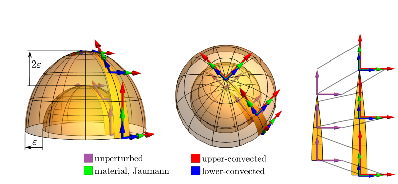
Figure 3: Strain deformation of a hemisphere (side and top view): If $\boldsymbol{X}$ parameterize the hemisphere $\mathcal{S}$, then, for $\boldsymbol{W}=\boldsymbol{\nu}+\boldsymbol{e}_{z}$, $\boldsymbol{X}_{\varepsilon}=\boldsymbol{X}+\varepsilon\boldsymbol{W}$ parameterize the strained hemispheroid $\mathcal{S}_{\varepsilon\boldsymbol{W}}$. Two orthogonal tangential vector fields (purple) of equal lengths are shown on a fixed longitude and three different latitudes at $\mathcal{S}$ exactly like in figure 2. The green, red and blue tangential vector fields are given on $\mathcal{S}_{\varepsilon}$ by pushing-forward the purple ones with the map $\mathcal{S}\rightarrow\mathcal{S}_{\varepsilon}$ assuming different gauges of surface independence respectively. The material and Jaumann gauge imply the same pushforward, since this is a pure strain deformation, i. e., the surface gradient of $\boldsymbol{W}$ is symmetric, cf. table 2. Gray parallel lines on the unrolled arc-length segment (right) indicate length preserving for pushforwarded vectors due to material and Jaumann gauges. By contrast, pushforwarded vectors, w. r. t. the upper- or lower convected gauge, are stretched along or against the deformation. However, the geometric mean of both yields the length preserved green vectors.

3.2.2 Consequences for Energy Variations

For a given state comprising the tangential vector field $\boldsymbol{q}[\boldsymbol{X}]$ and a parameterization $\boldsymbol{X}$, which fully determines the surface $\mathcal{S}$, the state energy $\mathfrak{U}[\boldsymbol{X},\boldsymbol{q}[\boldsymbol{X}]]\in\mathbb{R}$. This allows to define directional total variations of $\mathfrak{U}$ by

$$\left\langle\frac{\operatorname{\delta}\!\mathfrak{U}}{\operatorname{\delta}\!\boldsymbol{X}},\boldsymbol{W}\right\rangle_{\operatorname{L}^{\!2}(\tensor{\operatorname{T}\!}{}\mathbb{R}^{3}|_{\mathcal{S}})} :=\lim_{\varepsilon\rightarrow 0}\frac{\mathfrak{U}[\boldsymbol{X}+\varepsilon\boldsymbol{W},\boldsymbol{q}[\boldsymbol{X}+\varepsilon\boldsymbol{W}]]-\mathfrak{U}[\boldsymbol{X},\boldsymbol{q}[\boldsymbol{X}]]}{\varepsilon}\in\mathbb{R}\,\text{,}$$ (27)

$$\left\langle\frac{\operatorname{\delta}\!\mathfrak{U}}{\operatorname{\delta}\!\boldsymbol{q}},\boldsymbol{r}\right\rangle_{\operatorname{L}^{\!2}(\tensor{\operatorname{T}\!}{}\mathcal{S})} :=\lim_{\varepsilon\rightarrow 0}\frac{\mathfrak{U}[\boldsymbol{X},\boldsymbol{q}[\boldsymbol{X}]+\varepsilon\boldsymbol{r}]-\mathfrak{U}[\boldsymbol{X},\boldsymbol{q}[\boldsymbol{X}]]}{\varepsilon}\in\mathbb{R}$$ (28)

in arbitrary directions of $\boldsymbol{W}\in\tensor{\operatorname{T}\!}{}\mathbb{R}^{3}|_{\mathcal{S}}$ and $\boldsymbol{r}\in\tensor{\operatorname{T}\!}{}\mathcal{S}$. Variation (27) bears a subtle issue. The term $\mathfrak{U}[\boldsymbol{X}+\varepsilon\boldsymbol{W},\boldsymbol{q}[\boldsymbol{X}+\varepsilon\boldsymbol{W}]]$ is not determined, since $\boldsymbol{q}[\boldsymbol{X}+\varepsilon\boldsymbol{W}]\in\tensor{\operatorname{T}\!}{}\mathcal{S}_{\varepsilon\boldsymbol{W}}$ is not determined. However, a Taylor expansion at $\varepsilon=0$, w. r. t. the embedding space shows

$$\boldsymbol{q}[\boldsymbol{X}+\varepsilon\boldsymbol{W}] =\operatorname{\Pi}_{\tensor{\operatorname{T}\!}{}\mathcal{S}_{\varepsilon\boldsymbol{W}}}\boldsymbol{q}[\boldsymbol{X}+\varepsilon\boldsymbol{W}]$$

$$=\operatorname{\Pi}_{\tensor{\operatorname{T}\!}{}\mathcal{S}_{\varepsilon\boldsymbol{W}}}\left(\left(\boldsymbol{q}[\boldsymbol{X}]\right)^{*_{\varepsilon\boldsymbol{W}}}+\varepsilon\left(\frac{d}{d\varepsilon}\Big{|}_{\varepsilon=0}\boldsymbol{q}[\boldsymbol{X}+\varepsilon\boldsymbol{W}]\right)^{\!\!*_{\varepsilon\boldsymbol{W}}}+\mathcal{O}(\varepsilon^{2})\right)$$

where $*_{\varepsilon\boldsymbol{W}}:\tensor{\operatorname{T}\!}{}\mathbb{R}^{3}|_{\mathcal{S}}\rightarrow\tensor{\operatorname{T}\!}{}\mathbb{R}^{3}|_{\mathcal{S}_{\varepsilon\boldsymbol{W}}}$ is the simplest conceivable $\mathbb{R}^{3}$-pushforward for the map $\mathcal{S}\rightarrow\mathcal{S}_{\varepsilon\boldsymbol{W}}$ and is given by

$$\boldsymbol{Q}^{*_{\varepsilon\boldsymbol{W}}}(y^{1},y^{2}) :=Q^{I}(y^{1},y^{2})\boldsymbol{e}_{I}\in\tensor{\operatorname{T}\!}{{}_{(\boldsymbol{X}+\varepsilon\boldsymbol{W})(y^{1},y^{2})}}\mathbb{R}^{3}$$ (29)

for all vector fields $\boldsymbol{Q}\in\tensor{\operatorname{T}\!}{}\mathbb{R}^{3}|_{\mathcal{S}}$. The deformation derivative $\tensor*{\eth}{{}_{\boldsymbol{W}}}:\tensor{\operatorname{T}\!}{}\mathcal{S}\rightarrow\tensor{\operatorname{T}\!}{}\mathbb{R}^{3}|_{\mathcal{S}}$, defined in (22), and another partial Taylor expansion at $\operatorname{\Pi}_{\tensor{\operatorname{T}\!}{}\mathcal{S}_{\varepsilon\boldsymbol{W}}}\left(\boldsymbol{q}[\boldsymbol{X}]\right)^{*_{\varepsilon\boldsymbol{W}}}\in\tensor{\operatorname{T}\!}{}\mathcal{S}_{\varepsilon\boldsymbol{W}}$ of the energy $\mathfrak{U}$ w. r. t. to the deformed surface $\mathcal{S}_{\varepsilon\boldsymbol{W}}$ gives

$$\mathfrak{U}[\boldsymbol{X}+\varepsilon\boldsymbol{W},\boldsymbol{q}[\boldsymbol{X}+\varepsilon\boldsymbol{W}]]$$

$$=\mathfrak{U}[\boldsymbol{X}+\varepsilon\boldsymbol{W},\operatorname{\Pi}_{\tensor{\operatorname{T}\!}{}\mathcal{S}_{\varepsilon\boldsymbol{W}}}\left(\boldsymbol{q}[\boldsymbol{X}]\right)^{*_{\varepsilon\boldsymbol{W}}}+\varepsilon\operatorname{\Pi}_{\tensor{\operatorname{T}\!}{}\mathcal{S}_{\varepsilon\boldsymbol{W}}}\left(\tensor*{\eth}{{}_{\boldsymbol{W}}}\boldsymbol{q}[\boldsymbol{X}]\right)^{*_{\varepsilon\boldsymbol{W}}}+\mathcal{O}(\varepsilon^{2})]$$

$$=\mathfrak{U}[\boldsymbol{X}+\varepsilon\boldsymbol{W},\operatorname{\Pi}_{\tensor{\operatorname{T}\!}{}\mathcal{S}_{\varepsilon\boldsymbol{W}}}\left(\boldsymbol{q}[\boldsymbol{X}]\right)^{*_{\varepsilon\boldsymbol{W}}}]$$ (30)

$$\quad\quad+\varepsilon\left\langle\frac{\operatorname{\delta}\!\mathfrak{U}}{\operatorname{\delta}\!(\operatorname{\Pi}_{\tensor{\operatorname{T}\!}{}\mathcal{S}_{\varepsilon\boldsymbol{W}}}\boldsymbol{q}^{*_{\varepsilon\boldsymbol{W}}})},\operatorname{\Pi}_{\tensor{\operatorname{T}\!}{}\mathcal{S}_{\varepsilon\boldsymbol{W}}}\left(\tensor*{\eth}{{}_{\boldsymbol{W}}}\boldsymbol{q}[\boldsymbol{X}]\right)^{*_{\varepsilon\boldsymbol{W}}}\right\rangle_{\operatorname{L}^{\!2}(\tensor{\operatorname{T}\!}{}\mathcal{S}_{\varepsilon\boldsymbol{W}})}+\mathcal{O}(\varepsilon^{2})\,\text{,}$$

where we used the directional variation (28), w. r. t. tangential vector field $\operatorname{\Pi}_{\tensor{\operatorname{T}\!}{}\mathcal{S}_{\varepsilon\boldsymbol{W}}}\left(\boldsymbol{q}[\boldsymbol{X}]\right)^{*_{\varepsilon\boldsymbol{W}}}\in\tensor{\operatorname{T}\!}{}\mathcal{S}_{\varepsilon\boldsymbol{W}}$ in direction of $\operatorname{\Pi}_{\tensor{\operatorname{T}\!}{}\mathcal{S}_{\varepsilon\boldsymbol{W}}}\left(\tensor*{\eth}{{}_{\boldsymbol{W}}}\boldsymbol{q}[\boldsymbol{X}]\right)^{*_{\varepsilon\boldsymbol{W}}}\in\tensor{\operatorname{T}\!}{}\mathcal{S}_{\varepsilon\boldsymbol{W}}$, and properties of inner products. To relate the total variation (27), we define the partial variation

$$\left\langle\frac{\partial\mathfrak{U}}{\partial\boldsymbol{X}},\boldsymbol{W}\right\rangle_{\operatorname{L}^{\!2}(\tensor{\operatorname{T}\!}{}\mathbb{R}^{3}|_{\mathcal{S}})} :=\lim_{\varepsilon\rightarrow 0}\frac{\mathfrak{U}[\boldsymbol{X}+\varepsilon\boldsymbol{W},\operatorname{\Pi}_{\tensor{\operatorname{T}\!}{}\mathcal{S}_{\varepsilon\boldsymbol{W}}}\left(\boldsymbol{q}[\boldsymbol{X}]\right)^{*_{\varepsilon\boldsymbol{W}}}]-\mathfrak{U}[\boldsymbol{X},\boldsymbol{q}[\boldsymbol{X}]]}{\varepsilon}\in\mathbb{R}$$ (31)

in arbitrary directions of $\boldsymbol{W}\in\tensor{\operatorname{T}\!}{}\mathbb{R}^{3}|_{\mathcal{S}}$ w. r. t. $\operatorname{L}^{\!2}(\tensor{\operatorname{T}\!}{}\mathbb{R}^{3}|_{\mathcal{S}})$. In praxis, this derivative means that everything in $\mathfrak{U}$ has to be differentiated w. r. t. $\boldsymbol{X}$ except for $\boldsymbol{q}[\boldsymbol{X}]\in\tensor{\operatorname{T}\!}{}\mathcal{S}$ (incl. its frame). For instance, in the energy term $\int_{\mathcal{S}}\|\boldsymbol{q}[\boldsymbol{X}]\|^{2}_{\tensor{\operatorname{T}\!}{}\mathcal{S}}\mu[\boldsymbol{X}]$ only $\mu[\boldsymbol{X}]$ has to be differentiated. Using that $\operatorname{\Pi}_{\tensor{\operatorname{T}\!}{}\mathcal{S}_{\varepsilon\boldsymbol{W}}}\circ*_{\varepsilon\boldsymbol{W}}\rightarrow\operatorname{\Pi}_{\tensor{\operatorname{T}\!}{}\mathcal{S}}$ is valid for $\varepsilon\rightarrow 0$, the material deformation derivative (23) and substituting the Taylor expansion above into the total variation (27) yields

$$\left\langle\frac{\operatorname{\delta}\!\mathfrak{U}}{\operatorname{\delta}\!\boldsymbol{X}},\boldsymbol{W}\right\rangle_{\operatorname{L}^{\!2}(\tensor{\operatorname{T}\!}{}\mathbb{R}^{3}|_{\mathcal{S}})} =\left\langle\frac{\partial\mathfrak{U}}{\partial\boldsymbol{X}},\boldsymbol{W}\right\rangle_{\operatorname{L}^{\!2}(\tensor{\operatorname{T}\!}{}\mathbb{R}^{3}|_{\mathcal{S}})}+\left\langle\frac{\operatorname{\delta}\!\mathfrak{U}}{\operatorname{\delta}\!\boldsymbol{q}},\tensor*{\eth}{{}_{\boldsymbol{W}}^{\mathcal{S}}}\boldsymbol{q}[\boldsymbol{X}]\right\rangle_{\operatorname{L}^{\!2}(\tensor{\operatorname{T}\!}{}\mathcal{S})}\,\text{.}$$ (32)

Note that the material deformation derivative $\tensor*{\eth}{{}_{\boldsymbol{W}}^{\mathcal{S}}}\boldsymbol{q}[\boldsymbol{X}]\in\tensor{\operatorname{T}\!}{}\mathcal{S}$ in (32) depends on the chosen gauge of surface independence and can be obtained from the first row of table 2.

Some readers may be used to consider rather contravariant proxys of vector fields than an entire field with its frame. Hence, we give with (61) in appendix A.1 an equivalent identity w. r. t. to an energy $\widetilde{\mathfrak{U}}[\boldsymbol{X},q^{1}[\boldsymbol{X}],q^{2}[\boldsymbol{X}]]$, but in terms of a contravariant approach. Also treating the proxy of the metric tensor explicitly could be of advantage. For this purpose (63) in appendix A.2 gives an equivalent identity w. r. t. an energy $\widehat{\mathfrak{U}}[\boldsymbol{X},\boldsymbol{q}[\boldsymbol{X}],\{g_{ij}[\boldsymbol{X}]\}]$. We like to highlight that $\left\langle\frac{\operatorname{\delta}\!\mathfrak{U}}{\operatorname{\delta}\!\boldsymbol{X}},\boldsymbol{W}\right\rangle_{\operatorname{L}^{\!2}(\tensor{\operatorname{T}\!}{}\mathbb{R}^{3}|_{\mathcal{S}})}$ depends only on the semantical description of $\mathfrak{U}$ and the assumed gauge of independence. Even if we write the same energy in dependency of $[\boldsymbol{X},\{q^{i}[\boldsymbol{X}]\},\{q_{i}[\boldsymbol{X}]\},\boldsymbol{q}[\boldsymbol{X}],\{g^{ij}[\boldsymbol{X}]\},\{g_{ij}[\boldsymbol{X}]\},\boldsymbol{I\!I}[\boldsymbol{X}],\mathcal{H}[\boldsymbol{X}],\mathcal{K}[\boldsymbol{X}],\ldots]$ the result is still the same, which shows the advantage of total derivatives. This is also the reason to omit geometrical quantities other than $\boldsymbol{X}$ in the dependency list, since all of them are represented by $\boldsymbol{X}$ and would have the only effect to blow up formulas without an influence on the results.

Sometimes it could be difficult to calculate the partial variation of an energy without touching its tangential vector field argument. Or it is hard to obtain the total variation for the chosen gauge of surface independence, though it is much easier for another gauge. In such situations it could be helpful to use the identities

$$\left\langle\frac{\operatorname{\delta}\!\mathfrak{U}}{\operatorname{\delta}\!\boldsymbol{X}},\boldsymbol{W}\right\rangle_{\operatorname{L}^{\!2}(\tensor{\operatorname{T}\!}{}\mathbb{R}^{3}|_{\mathcal{S}})} =\left\langle\frac{\operatorname{\delta}\!\mathfrak{U}}{\operatorname{\delta}\!\boldsymbol{X}}\Big{|}_{\tensor*{\eth}{{}^{\Psi}}\boldsymbol{q}=0},\boldsymbol{W}\right\rangle_{\operatorname{L}^{\!2}(\tensor{\operatorname{T}\!}{}\mathbb{R}^{3}|_{\mathcal{S}})}+\left\langle\frac{\operatorname{\delta}\!\mathfrak{U}}{\operatorname{\delta}\!\boldsymbol{q}},\tensor*{\eth}{{}_{\boldsymbol{W}}^{\Psi}}\boldsymbol{q}[\boldsymbol{X}]\right\rangle_{\operatorname{L}^{\!2}(\tensor{\operatorname{T}\!}{}\mathcal{S})}$$ (33)

$$\left\langle\frac{\partial\mathfrak{U}}{\partial\boldsymbol{X}},\boldsymbol{W}\right\rangle_{\operatorname{L}^{\!2}(\tensor{\operatorname{T}\!}{}\mathbb{R}^{3}|_{\mathcal{S}})} =\left\langle\frac{\operatorname{\delta}\!\mathfrak{U}}{\operatorname{\delta}\!\boldsymbol{X}}\Big{|}_{\tensor*{\eth}{{}^{\Psi}}\boldsymbol{q}=0},\boldsymbol{W}\right\rangle_{\operatorname{L}^{\!2}(\tensor{\operatorname{T}\!}{}\mathbb{R}^{3}|_{\mathcal{S}})}+\left\langle\frac{\operatorname{\delta}\!\mathfrak{U}}{\operatorname{\delta}\!\boldsymbol{q}},\tensor*{\eth}{{}_{\boldsymbol{W}}^{\Psi}}\boldsymbol{q}[\boldsymbol{X}]-\tensor*{\eth}{{}_{\boldsymbol{W}}^{\mathcal{S}}}\boldsymbol{q}[\boldsymbol{X}]\right\rangle_{\operatorname{L}^{\!2}(\tensor{\operatorname{T}\!}{}\mathcal{S})},$$ (34)

where the symbol $\Psi\in\{\mathcal{S},\sharp,\flat,\mathcal{J}\}$ determine the desired deformation derivative. We get both identities by using (32) and the fact that the partial variation (31) does not depend on any gauge. Moreover, (33) generalizes (32) in the sense that (33) equals (32) for $\Psi=\mathcal{S}$, since $\frac{\operatorname{\delta}\!\mathfrak{U}}{\operatorname{\delta}\!\boldsymbol{X}}\big{|}_{\tensor*{\eth}{{}^{\mathcal{S}}}{}\boldsymbol{q}=0}=\frac{\partial\mathfrak{U}}{\partial\boldsymbol{X}}$.

3.2.3 Consequences for $\operatorname{L}^{\!2}$-Gradients

The $\operatorname{L}^{\!2}$-gradient is weakly given by

$$\left\langle\nabla_{\operatorname{L}^{\!2}}\mathfrak{U},(\boldsymbol{W},\boldsymbol{r})\right\rangle_{\operatorname{L}^{\!2}(\tensor{\operatorname{T}\!}{}\mathbb{R}^{3}|_{\mathcal{S}}\times\tensor{\operatorname{T}\!}{}\mathcal{S})} :=\left\langle\frac{\operatorname{\delta}\!\mathfrak{U}}{\operatorname{\delta}\!\boldsymbol{X}},\boldsymbol{W}\right\rangle_{\operatorname{L}^{\!2}(\tensor{\operatorname{T}\!}{}\mathbb{R}^{3}|_{\mathcal{S}})}+\left\langle\frac{\operatorname{\delta}\!\mathfrak{U}}{\operatorname{\delta}\!\boldsymbol{q}},\boldsymbol{r}\right\rangle_{\operatorname{L}^{\!2}(\tensor{\operatorname{T}\!}{}\mathcal{S})}$$

for all $(\boldsymbol{W},\boldsymbol{r})\in\tensor{\operatorname{T}\!}{}\mathbb{R}^{3}|_{\mathcal{S}}\times\tensor{\operatorname{T}\!}{}\mathcal{S}$. Considering (32) and a chosen gauge of independence for $\boldsymbol{q}[\boldsymbol{X}]\in\tensor{\operatorname{T}\!}{}\mathcal{S}$, we get

$$\left\langle\nabla_{\operatorname{L}^{\!2}}\mathfrak{U},(\boldsymbol{W},\boldsymbol{r})\right\rangle_{\operatorname{L}^{\!2}(\tensor{\operatorname{T}\!}{}\mathbb{R}^{3}|_{\mathcal{S}}\times\tensor{\operatorname{T}\!}{}\mathcal{S})}$$

$$\quad\quad=\left\langle\frac{\partial\mathfrak{U}}{\partial\boldsymbol{X}},\boldsymbol{W}\right\rangle_{\operatorname{L}^{\!2}(\tensor{\operatorname{T}\!}{}\mathbb{R}^{3}|_{\mathcal{S}})}+\left\langle\frac{\operatorname{\delta}\!\mathfrak{U}}{\operatorname{\delta}\!\boldsymbol{q}},\boldsymbol{r}+\boldsymbol{\Psi}[\boldsymbol{X},\boldsymbol{W}]\boldsymbol{q}[\boldsymbol{X}]\right\rangle_{\operatorname{L}^{\!2}(\tensor{\operatorname{T}\!}{}\mathcal{S})}\,\text{,}$$ (35)

where	$\boldsymbol{\Psi}=$	$0$	$\boldsymbol{G}$	$-\boldsymbol{G}^{T}$	$\boldsymbol{A}$
for	$0=$	$\tensor*{\eth}{{}^{\mathcal{S}}}\boldsymbol{q}$	$\tensor*{\eth}{{}^{\sharp}}\boldsymbol{q}$	$\tensor*{\eth}{{}^{\flat}}\boldsymbol{q}$	$\tensor*{\eth}{{}^{\mathcal{J}}}\boldsymbol{q}$

according to the first row in table 2. The strong formulation of the $\operatorname{L}^{\!2}$-gradient reads

$$\nabla_{\operatorname{L}^{\!2}}\mathfrak{U} =\left(\frac{\operatorname{\delta}\!\mathfrak{U}}{\operatorname{\delta}\!\boldsymbol{X}},\frac{\operatorname{\delta}\!\mathfrak{U}}{\operatorname{\delta}\!\boldsymbol{q}}\right)=\left(\frac{\partial\mathfrak{U}}{\partial\boldsymbol{X}}-\operatorname{div}_{\tensor{\operatorname{T}\!}{{}^{2}}\mathcal{S}}\boldsymbol{\sigma},\frac{\operatorname{\delta}\!\mathfrak{U}}{\operatorname{\delta}\!\boldsymbol{q}}\right)\in\tensor{\operatorname{T}\!}{}\mathbb{R}^{3}|_{\mathcal{S}}\times\tensor{\operatorname{T}\!}{}\mathcal{S}\,\text{,}$$ (36)

where we used (35), the deformation-$\operatorname{L}^{\!2}$-adjoints $\boldsymbol{\Psi}^{\ddagger}[\boldsymbol{X}]$ given in (15) and the gauge stress tensor fields $\boldsymbol{\sigma}\in\tensor{\operatorname{T}\!}{{}^{2}}\mathcal{S}$, which are depending on the chosen gauge and given in the first row of table 3. In an equation of motion containing $\nabla_{\operatorname{L}^{\!2}}\mathfrak{U}$, e. g., in the $\operatorname{L}^{\!2}$-gradient flow in the subsection below, the term $\operatorname{div}_{\tensor{\operatorname{T}\!}{{}^{2}}\mathcal{S}}\boldsymbol{\sigma}=\operatorname{div}\boldsymbol{\sigma}+\left\langle\boldsymbol{I\!I}[\boldsymbol{X}],\boldsymbol{\sigma}\right\rangle\boldsymbol{\nu}\in\tensor{\operatorname{T}\!}{}\mathbb{R}^{3}|_{\mathcal{S}}$ can be interpreted as a partial force induced by the chosen gauge of surface independence. We name the resulting force “partial”, since $\boldsymbol{\sigma}$ depends on the syntactical description of $\mathfrak{U}$. For instance, if we use an equivalent contravariant approach $\widetilde{\mathfrak{U}}[\boldsymbol{X},q^{1}[\boldsymbol{X}],q^{2}[\boldsymbol{X}]]=\mathfrak{U}[\boldsymbol{X},\boldsymbol{q}[\boldsymbol{X}]]$, as given in appendix A.1, we see in (62) that we end up with a gauge stress field $\widetilde{\boldsymbol{\sigma}}=\boldsymbol{\sigma}-\frac{\operatorname{\delta}\!\mathfrak{U}}{\operatorname{\delta}\!\boldsymbol{q}}\otimes\boldsymbol{q}[\boldsymbol{X}]\in\tensor{\operatorname{T}\!}{{}^{2}}\mathcal{S}$, see second row in table 3. Note that the approach in appendix A.2, where we treat the metric proxy explicitly by $\widehat{\mathfrak{U}}[\boldsymbol{X},\boldsymbol{q}[\boldsymbol{X}],\{g_{ij}[\boldsymbol{X}]\}]=\mathfrak{U}[\boldsymbol{X},\boldsymbol{q}[\boldsymbol{X}]]$ and using the term $\frac{\partial\widehat{\mathfrak{U}}}{\partial\boldsymbol{X}}$ instead $\frac{\partial\mathfrak{U}}{\partial\boldsymbol{X}}$, yields the stress tensor fields $\widehat{\boldsymbol{\sigma}}=\boldsymbol{\sigma}+\frac{\partial\widehat{\mathfrak{U}}}{\partial g_{ij}}\partial_{i}\boldsymbol{X}\otimes\partial_{j}\boldsymbol{X}$.

	$\tensor*{\eth}{{}^{\mathcal{S}}}\boldsymbol{q}=0$	$\tensor*{\eth}{{}^{\sharp}}\boldsymbol{q}=0$	$\tensor*{\eth}{{}^{\flat}}\boldsymbol{q}=0$	$\tensor*{\eth}{{}^{\mathcal{J}}}\boldsymbol{q}=0$
	(Definition 2)	(Definition 3)	(Definition 4)	(Definition 5)
$\boldsymbol{\sigma}$	$0$	$\frac{\operatorname{\delta}\!\mathfrak{U}}{\operatorname{\delta}\!\boldsymbol{q}}\otimes\boldsymbol{q}[\boldsymbol{X}]$	$-\boldsymbol{q}[\boldsymbol{X}]\otimes\frac{\operatorname{\delta}\!\mathfrak{U}}{\operatorname{\delta}\!\boldsymbol{q}}$	$\frac{\operatorname{\delta}\!\mathfrak{U}}{\operatorname{\delta}\!\boldsymbol{q}}\owedge\boldsymbol{q}[\boldsymbol{X}]$
$\widetilde{\boldsymbol{\sigma}}$	$-\frac{\operatorname{\delta}\!\widetilde{\mathfrak{U}}}{\operatorname{\delta}\!\boldsymbol{q}}\otimes\boldsymbol{q}[\boldsymbol{X}]$	$0$	$-2\frac{\operatorname{\delta}\!\widetilde{\mathfrak{U}}}{\operatorname{\delta}\!\boldsymbol{q}}\ovee\boldsymbol{q}[\boldsymbol{X}]$	$-\frac{\operatorname{\delta}\!\widetilde{\mathfrak{U}}}{\operatorname{\delta}\!\boldsymbol{q}}\ovee\boldsymbol{q}[\boldsymbol{X}]$

Table 3: Gauge stress tensor fields $\boldsymbol{\sigma},\widetilde{\boldsymbol{\sigma}}\in\tensor{\operatorname{T}\!}{{}^{2}}\mathcal{S}$ caused by different gauges of surface independence. $\boldsymbol{\sigma}$, resp. $\widetilde{\boldsymbol{\sigma}}$, apply in (36) and (54), resp. (62), according to syntactically stipulated partial dependency in the energy $\mathfrak{U}$, or $\widetilde{\mathfrak{U}}$. We define anti- and symmetric outer products by $2\boldsymbol{r}\owedge\boldsymbol{q}:=\boldsymbol{r}\otimes\boldsymbol{q}-\boldsymbol{q}\otimes\boldsymbol{r}$ and $2\boldsymbol{r}\ovee\boldsymbol{q}:=\boldsymbol{r}\otimes\boldsymbol{q}+\boldsymbol{q}\otimes\boldsymbol{r}$ for all $\boldsymbol{r},\boldsymbol{q}\in\tensor{\operatorname{T}\!}{}\mathcal{S}$.

Remark 1.

The solutions of the stationary equation $0=\nabla_{\operatorname{L}^{\!2}}\mathfrak{U}$ do not depend on any gauge of surface independence. On the one hand $\frac{\partial\mathfrak{U}}{\partial\boldsymbol{X}}$ does not depend on a gauge. On the other hand at a local extremum of $\mathfrak{U}$, where $\frac{\operatorname{\delta}\!\mathfrak{U}}{\operatorname{\delta}\!\boldsymbol{q}}=0$ is valid, all gauge stress tensors fields $\boldsymbol{\sigma}$ are vanishing.

3.2.4 Consequences for $\operatorname{L}^{\!2}$-Gradient Flows

In general, the strong formulation of the $\operatorname{L}^{\!2}$-gradient flow reads

$$\left(\frac{d}{dt}\boldsymbol{X},\mathfrak{D_{t}}\boldsymbol{q}[\boldsymbol{X}]\right) =-\lambda\nabla_{\operatorname{L}^{\!2}}\mathfrak{U}\,\text{,}$$ (37)

where $\lambda>0$ is a mobility parameter coefficient and $\mathfrak{D_{t}}\boldsymbol{q}[\boldsymbol{X}]\in\tensor{\operatorname{T}\!}{}\mathcal{S}$ an observer-invariant instantaneous time derivative of $\boldsymbol{q}[\boldsymbol{X}]\in\tensor{\operatorname{T}\!}{}\mathcal{S}$ given in (Nitschke_2022, , Conclusion 6). We consider the material, upper-convected, lower-convected and Jaumann time derivative in this context. At this, the parameterization $\boldsymbol{X}$ is time-depending, as well as the tangential vector field $\boldsymbol{q}[\boldsymbol{X}]\in\tensor{\operatorname{T}\!}{}\mathcal{S}$ by $\boldsymbol{X}$ and also partially in $t$, i. e., at an event $(t,\boldsymbol{X}|_{t}(y^{1},y^{2}))\in\mathbb{R}\times\mathcal{S}|_{t}\subset\mathbb{R}^{4}$ describes $\boldsymbol{X}(t,y^{1},y^{2}):=\boldsymbol{X}|_{t}(y^{1},y^{2})\in\mathcal{S}|_{t}$ the spatial location and $\boldsymbol{q}[\boldsymbol{X}](t,y^{1},y^{2})=(\boldsymbol{q}[\boldsymbol{X}](y^{1},y^{2}))|_{t}\in\tensor{\operatorname{T}\!}{{}_{\boldsymbol{X}|_{t}(y^{1},y^{2})}}\mathcal{S}|_{t}$ the state of the vector field. We assume that the energy $\mathfrak{U}$ is instantaneous and not partially time depending, i. e., $\mathfrak{U}$ does not depend on any rates of $\boldsymbol{X}$ or $\boldsymbol{q}[\boldsymbol{X}]$ and it holds $(\mathfrak{U}[\boldsymbol{X},\boldsymbol{q}[\boldsymbol{X}]])|_{t}=\mathfrak{U}[\boldsymbol{X}|_{t},(\boldsymbol{q}[\boldsymbol{X}])|_{t}]$, which is common for potential or free energies. We omit the affix $|_{t}$ if it is clear that quantities are given at time $t$.

Note that the time depending parameterization $\boldsymbol{X}$ can be any observer parameterization for the time depending surface $\mathcal{S}$. This also includes the material parameterization $\boldsymbol{X}_{\mathfrak{m}}$, where $\boldsymbol{X}_{\mathfrak{m}}|_{(y^{1}_{\mathfrak{m}},y^{1}_{\mathfrak{m}})}(t)$ describes the world line of one material particle. While the material parameterization takes the Lagrange perspective, the observer parameterization $\boldsymbol{X}_{\mathfrak{o}}$ is an arbitrary parameterization taking the observer perspective, i. e., $\boldsymbol{X}_{\mathfrak{o}}|_{(y^{1}_{\mathfrak{o}},y^{1}_{\mathfrak{o}})}(t)$ describes the world line of an observer particle, see Nitschke_2022 . The left-hand side of (37) depends on the dynamic of the material, but we are able to formulate it invariant of an observer. The first component is the material velocity field $\boldsymbol{V}_{\mathfrak{m}}[\boldsymbol{X}_{\mathfrak{m}}]:=\frac{d}{dt}\boldsymbol{X}_{\mathfrak{o}}=\partial_{t}\boldsymbol{X}_{\mathfrak{m}}\in\tensor{\operatorname{T}\!}{}\mathbb{R}^{3}|_{\mathcal{S}}$. Whereas $\boldsymbol{V}_{\mathfrak{o}}[\boldsymbol{X}_{\mathfrak{o}}]:=\partial_{t}\boldsymbol{X}_{\mathfrak{o}}\in\tensor{\operatorname{T}\!}{}\mathbb{R}^{3}|_{\mathcal{S}}$ is the observer velocity field. From observer perspective, both velocity fields can be related by the relative velocity $\boldsymbol{u}[\boldsymbol{X}_{\mathfrak{o}},\boldsymbol{X}_{\mathfrak{m}}](t,y^{1}_{\mathfrak{o}},y^{1}_{\mathfrak{o}}):=\boldsymbol{V}_{\mathfrak{m}}^{\mathfrak{o}}[\boldsymbol{X}_{\mathfrak{o}},\boldsymbol{X}_{\mathfrak{m}}](t,y^{1}_{\mathfrak{o}},y^{1}_{\mathfrak{o}})-\boldsymbol{V}_{\mathfrak{o}}[\boldsymbol{X}_{\mathfrak{o}}](t,y^{1}_{\mathfrak{o}},y^{1}_{\mathfrak{o}})$, where $\boldsymbol{V}_{\mathfrak{m}}^{\mathfrak{o}}[\boldsymbol{X}_{\mathfrak{o}},\boldsymbol{X}_{\mathfrak{m}}](t,y^{1}_{\mathfrak{o}},y^{1}_{\mathfrak{o}}):=\boldsymbol{V}_{\mathfrak{m}}[\boldsymbol{X}_{\mathfrak{m}}](t,(\boldsymbol{X}_{\mathfrak{m}}|_{t})^{-1}(\boldsymbol{X}_{\mathfrak{o}}(t,y^{1}_{\mathfrak{o}},y^{1}_{\mathfrak{o}})))$ is the material velocity evaluated at observer location $\boldsymbol{X}_{\mathfrak{o}}(t,y^{1}_{\mathfrak{o}},y^{1}_{\mathfrak{o}})$. Note that for the relative velocity field holds $\boldsymbol{u}[\boldsymbol{X}_{\mathfrak{o}},\boldsymbol{X}_{\mathfrak{m}}]\in\tensor{\operatorname{T}\!}{}\mathcal{S}$, since the normal part of the observer and material velocity is equal. Therefore, the material time derivative of $\boldsymbol{q}[\boldsymbol{X}_{\mathfrak{o}}]\in\tensor{\operatorname{T}\!}{}\mathcal{S}$ is given by

$$\dot{\boldsymbol{q}}[\boldsymbol{X}_{\mathfrak{o}}] =(\partial_{t}q^{i}[\boldsymbol{X}_{\mathfrak{o}}])\partial_{i}\boldsymbol{X}_{\mathfrak{o}}+\nabla_{\boldsymbol{u}[\boldsymbol{X}_{\mathfrak{o}},\boldsymbol{X}_{\mathfrak{m}}]}\boldsymbol{q}[\boldsymbol{X}_{\mathfrak{o}}]+\boldsymbol{G}[\boldsymbol{X}_{\mathfrak{o}},\boldsymbol{V}_{\mathfrak{o}}[\boldsymbol{X}_{\mathfrak{o}}]]\boldsymbol{q}[\boldsymbol{X}_{\mathfrak{o}}]$$

$$=\operatorname{\Pi}_{\tensor{\operatorname{T}\!}{}\mathcal{S}}\frac{d}{dt}\boldsymbol{q}[\boldsymbol{X}_{\mathfrak{o}}]\,\text{,}$$

where the rear identity is a conclusion in (Nitschke_2022, , Proposition 4). All considered time derivatives can be derived from the material one by

$$\mathfrak{D_{t}}\boldsymbol{q}[\boldsymbol{X}_{\mathfrak{o}}] =\dot{\boldsymbol{q}}[\boldsymbol{X}_{\mathfrak{o}}]-\boldsymbol{\Phi}[\boldsymbol{X}_{\mathfrak{o}},\boldsymbol{V}_{\mathfrak{m}}^{\mathfrak{o}}[\boldsymbol{X}_{\mathfrak{o}},\boldsymbol{X}_{\mathfrak{m}}]]\boldsymbol{q}[\boldsymbol{X}_{\mathfrak{o}}]\,\text{,}$$ (38)

where	$\mathfrak{D_{t}}\boldsymbol{q}=$	$\dot{\boldsymbol{q}}$	$\mathfrak{L}^{\sharp}\boldsymbol{q}$	$\mathfrak{L}^{\flat}\boldsymbol{q}$	$\mathfrak{J}\boldsymbol{q}$
for	$\boldsymbol{\Phi}=$	$0$	$\boldsymbol{G}$	$-\boldsymbol{G}^{T}$	$\boldsymbol{A}$	,

where $\mathfrak{L}^{\sharp}$ is the upper-convected, $\mathfrak{L}^{\flat}$ the lower-convected and $\mathfrak{J}$ the Jaumann time derivative on tangential vector fields, see Nitschke_2022 .

Since the left-handed side of (37) is observer-invariant and the right-handed side is instantaneous, we take the Lagrange perspective in the following without loss of generality. This means that we set $\boldsymbol{X}:=\boldsymbol{X}_{\mathfrak{o}}=\boldsymbol{X}_{\mathfrak{m}}$. Due to this it is $\boldsymbol{V}[\boldsymbol{X}]:=\boldsymbol{V}_{\mathfrak{m}}[\boldsymbol{X}_{\mathfrak{m}}]=\boldsymbol{V}_{\mathfrak{m}}^{\mathfrak{o}}[\boldsymbol{X}_{\mathfrak{o}},\boldsymbol{X}_{\mathfrak{m}}]=\boldsymbol{V}_{\mathfrak{o}}[\boldsymbol{X}_{\mathfrak{o}}]$ and $\boldsymbol{u}[\boldsymbol{X}_{\mathfrak{o}},\boldsymbol{X}_{\mathfrak{m}}]=0$ valid.

The time derivative of the energy $\mathfrak{U}$ gives the energy rate

$$\frac{d}{dt}\mathfrak{U} :=\lim_{\varepsilon\rightarrow 0}\frac{(\mathfrak{U}[\boldsymbol{X},\boldsymbol{q}[\boldsymbol{X}]])|_{t+\varepsilon}-(\mathfrak{U}[\boldsymbol{X},\boldsymbol{q}[\boldsymbol{X}]])|_{t}}{\varepsilon}$$

$$=\left\langle\frac{\partial\mathfrak{U}}{\partial\boldsymbol{X}},\boldsymbol{V}[\boldsymbol{X}]\right\rangle_{\operatorname{L}^{\!2}(\tensor{\operatorname{T}\!}{}\mathbb{R}^{3}|_{\mathcal{S}})}+\left\langle\frac{\operatorname{\delta}\!\mathfrak{U}}{\operatorname{\delta}\!\boldsymbol{q}},\dot{\boldsymbol{q}}[\boldsymbol{X}]\right\rangle_{\operatorname{L}^{\!2}(\tensor{\operatorname{T}\!}{}\mathcal{S})}\,\text{.}$$

This can be obtained by Taylor expansions at $\epsilon=0$, similarly to (30) for $\boldsymbol{W}=\boldsymbol{V}[\boldsymbol{X}]+\mathcal{O}(\varepsilon)$. A priori, the energy rate is invariant w. r. t. any chosen gauges of independence. This behavior changes if we substitute the gauge-depended gradient flow (37) into this rate. With (32) we get

$$\frac{d}{dt}\mathfrak{U} =\left\langle\frac{\operatorname{\delta}\!\mathfrak{U}}{\operatorname{\delta}\!\boldsymbol{X}},\boldsymbol{V}[\boldsymbol{X}]\right\rangle_{\operatorname{L}^{\!2}(\tensor{\operatorname{T}\!}{}\mathbb{R}^{3}|_{\mathcal{S}})}+\left\langle\frac{\operatorname{\delta}\!\mathfrak{U}}{\operatorname{\delta}\!\boldsymbol{q}},\dot{\boldsymbol{q}}[\boldsymbol{X}]-\tensor*{\eth}{{}_{\boldsymbol{V}[\boldsymbol{X}]}^{\mathcal{S}}}\boldsymbol{q}[\boldsymbol{X}]\right\rangle_{\operatorname{L}^{\!2}(\tensor{\operatorname{T}\!}{}\mathcal{S})}$$

$$=\left\langle\frac{\operatorname{\delta}\!\mathfrak{U}}{\operatorname{\delta}\!\boldsymbol{X}},\boldsymbol{V}[\boldsymbol{X}]\right\rangle_{\operatorname{L}^{\!2}(\tensor{\operatorname{T}\!}{}\mathbb{R}^{3}|_{\mathcal{S}})}+\left\langle\frac{\operatorname{\delta}\!\mathfrak{U}}{\operatorname{\delta}\!\boldsymbol{q}},\mathfrak{D_{t}}\boldsymbol{q}[\boldsymbol{X}]+(\boldsymbol{\Phi}-\boldsymbol{\Psi})[\boldsymbol{X},\boldsymbol{V}[\boldsymbol{X}]]\boldsymbol{q}[\boldsymbol{X}]\right\rangle_{\operatorname{L}^{\!2}(\tensor{\operatorname{T}\!}{}\mathcal{S})}$$ (39)

$$=-\lambda\left\|\nabla_{\operatorname{L}^{\!2}}\mathfrak{U}\right\|_{\operatorname{L}^{\!2}(\tensor{\operatorname{T}\!}{}\mathbb{R}^{3}|_{\mathcal{S}}\times\tensor{\operatorname{T}\!}{}\mathcal{S})}^{2}+\left\langle\frac{\operatorname{\delta}\!\mathfrak{U}}{\operatorname{\delta}\!\boldsymbol{q}},(\boldsymbol{\Phi}-\boldsymbol{\Psi})[\boldsymbol{X},\boldsymbol{V}[\boldsymbol{X}]]\boldsymbol{q}[\boldsymbol{X}]\right\rangle_{\operatorname{L}^{\!2}(\tensor{\operatorname{T}\!}{}\mathcal{S})}\,\text{,}$$ (40)

where $\boldsymbol{\Psi}[\boldsymbol{X},\boldsymbol{V}[\boldsymbol{X}]]\in\tensor{\operatorname{T}\!}{{}^{2}}\mathcal{S}$ is already introduced in (35) and depends on the chosen gauge, cf. the header in table 4. Using a time derivative in the gradient flow (37), which name is consistent to the chosen gauge, e. g., upper-convected time derivative for a upper-convected gauge, is sufficient to ensure a dissipative energy, i. e., it holds $\frac{d}{dt}\mathfrak{U}\leq 0$, since $(\boldsymbol{\Phi}-\boldsymbol{\Psi})[\boldsymbol{X},\boldsymbol{V}[\boldsymbol{X}]]=0$ is valid. In contrast, using time derivatives and gauges inconsistently in their names, e. g., material time derivative and Jaumann gauge, could rise an issue for the dissipation, especially for small $\lambda$. However, we present in table 4 all 16 possible combinations we discussed.

		$\tensor*{\eth}{{}^{\mathcal{S}}}\boldsymbol{q}=0$	$\tensor*{\eth}{{}^{\sharp}}\boldsymbol{q}=0$	$\tensor*{\eth}{{}^{\flat}}\boldsymbol{q}=0$	$\tensor*{\eth}{{}^{\mathcal{J}}}\boldsymbol{q}=0$
$(\boldsymbol{\Phi}-\boldsymbol{\Psi})[\boldsymbol{X},\boldsymbol{V}[\boldsymbol{X}]]$		(Definition2)	(Definition 3)	(Definition 4)	(Definition 5)
		$\Rightarrow\boldsymbol{\Psi}=0$	$\Rightarrow\boldsymbol{\Psi}=\boldsymbol{G}$	$\Rightarrow\boldsymbol{\Psi}=-\boldsymbol{G}^{T}$	$\Rightarrow\boldsymbol{\Psi}=\boldsymbol{A}$
$\dot{\boldsymbol{q}}[\boldsymbol{X}]$	$\Rightarrow\boldsymbol{\Phi}=0$	$0$	$-\boldsymbol{G}[\boldsymbol{X},\boldsymbol{V}[\boldsymbol{X}]]$	$\boldsymbol{G}^{T}[\boldsymbol{X},\boldsymbol{V}[\boldsymbol{X}]]$	$-\boldsymbol{A}[\boldsymbol{X},\boldsymbol{V}[\boldsymbol{X}]]$
$\mathfrak{L}^{\sharp}\boldsymbol{q}[\boldsymbol{X}]$	$\Rightarrow\boldsymbol{\Phi}=\boldsymbol{G}$	$\boldsymbol{G}[\boldsymbol{X},\boldsymbol{V}[\boldsymbol{X}]]$	$0$	$2\boldsymbol{S}[\boldsymbol{X},\boldsymbol{V}[\boldsymbol{X}]]$	$\boldsymbol{S}[\boldsymbol{X},\boldsymbol{V}[\boldsymbol{X}]]$
$\mathfrak{L}^{\flat}\boldsymbol{q}[\boldsymbol{X}]$	$\Rightarrow\boldsymbol{\Phi}=-\boldsymbol{G}^{T}$	$-\boldsymbol{G}^{T}[\boldsymbol{X},\boldsymbol{V}[\boldsymbol{X}]]$	$-2\boldsymbol{S}[\boldsymbol{X},\boldsymbol{V}[\boldsymbol{X}]]$	$0$	$-\boldsymbol{S}[\boldsymbol{X},\boldsymbol{V}[\boldsymbol{X}]]$
$\mathfrak{J}\boldsymbol{q}[\boldsymbol{X}]$	$\Rightarrow\boldsymbol{\Phi}=\boldsymbol{A}$	$\boldsymbol{A}[\boldsymbol{X},\boldsymbol{V}[\boldsymbol{X}]]$	$-\boldsymbol{S}[\boldsymbol{X},\boldsymbol{V}[\boldsymbol{X}]]$	$\boldsymbol{S}[\boldsymbol{X},\boldsymbol{V}[\boldsymbol{X}]]$	$0$

Table 4: Determining $(\boldsymbol{\Phi}-\boldsymbol{\Psi})[\boldsymbol{X},\boldsymbol{V}[\boldsymbol{X}]]\in\tensor{\operatorname{T}\!}{{}^{2}}\mathcal{S}$ in the rear term of energy rate (40) by combinations of different chosen gauges of surface independence (columns) and time derivatives (rows). From left to right, resp. top to bottom, it is material, upper-convected, lower-convected, Jaumann gauge, resp. time derivative, considered. For definitions of $\boldsymbol{G},\boldsymbol{S}$ and $\boldsymbol{A}$ see table 1 and for time derivatives (Nitschke_2022, , Conclusion 6). Note that $\boldsymbol{V}$ is the material as well as the observer velocity.

Remark 2.

Using the Onsagers variational principle Doi to obtain the gradient flow (37) is forcing a consistence choice of time derivative and gauge of surface independence.

This follows by minimizing the Rayleighian

$$\mathfrak{R}[\boldsymbol{V},\mathfrak{D_{t}}\boldsymbol{q}] :=\frac{1}{2\lambda}\left(\left\|\boldsymbol{V}\right\|_{\operatorname{L}^{\!2}(\tensor{\operatorname{T}\!}{}\mathbb{R}^{3}|_{\mathcal{S}})}^{2}+\left\|\mathfrak{D_{t}}\boldsymbol{q}\right\|_{\operatorname{L}^{\!2}(\tensor{\operatorname{T}\!}{}\mathbb{R}^{3}|_{\mathcal{S}})}^{2}\right)+(\frac{d}{dt}\mathfrak{U})[\boldsymbol{V},\mathfrak{D_{t}}\boldsymbol{q}]$$

by the necessary condition $(0,0)=(\frac{\operatorname{\delta}\!\mathfrak{R}}{\operatorname{\delta}\!\boldsymbol{V}},\frac{\operatorname{\delta}\!\mathfrak{R}}{\operatorname{\delta}\!(\mathfrak{D_{t}}\boldsymbol{q})})$, with an energy rate $\frac{d}{dt}\mathfrak{U}$ given in (39) w. r. t. process variables $\boldsymbol{V}$ and $\mathfrak{D_{t}}\boldsymbol{q}$. As a consequence, $(\boldsymbol{\Phi}-\boldsymbol{\Psi})[\boldsymbol{X},\boldsymbol{V}[\boldsymbol{X}]]=0$ has to be valid by comparison with the gradient flow (37).

In section 4.2 we provide an example for a Frank-Oseen energy, derive the $\operatorname{L}^{\!2}$-gradient flow and demonstrate differences of the consistent combinations in table 4.

3.3 Tangential 2-Tensor Fields

The proceeding is almost the same as for tangential vector fields in section 3.2. Therefore we keep the argumentation much shorter in this section.

3.3.1 Gauges of Surface Independence

A tangential 2-tensor field $\boldsymbol{q}[\boldsymbol{X}]\in\tensor{\operatorname{T}\!}{{}^{2}}\mathcal{S}$ can be represented in a tangential as well as the Euclidean frame, i. e., it holds $\boldsymbol{q}[\boldsymbol{X}]=q^{ij}[\boldsymbol{X}]\partial_{i}\boldsymbol{X}\otimes\partial_{j}\boldsymbol{X}=q^{IJ}[\boldsymbol{X}]\boldsymbol{e}_{I}\otimes\boldsymbol{e}_{J}$. Since $\boldsymbol{e}_{I}$ does not depend on the surface in any way, we define and calculate

$$\tensor*{\eth}{{}_{\boldsymbol{W}}}\boldsymbol{q}[\boldsymbol{X}] :=\left(\tensor*{\eth}{{}_{\boldsymbol{W}}}q^{IJ}[\boldsymbol{X}]\right)\boldsymbol{e}_{I}\otimes\boldsymbol{e}_{J}$$

$$=\left(\tensor*{\eth}{{}_{\boldsymbol{W}}}q^{ij}[\boldsymbol{X}]\right)\partial_{i}\boldsymbol{X}\otimes\partial_{j}\boldsymbol{X}+q^{ij}[\boldsymbol{X}]\left(\partial_{i}\boldsymbol{W}\otimes\partial_{j}\boldsymbol{X}+\partial_{i}\boldsymbol{X}\otimes\partial_{j}\boldsymbol{W}\right)$$ (41)

w. r. t. the deformation derivative (17) on scalar fields. The derivative (41) maps to $\tensor{\operatorname{T}\!}{{}^{2}}\mathbb{R}^{3}|_{\mathcal{S}}$, but all non-tangential parts of the image are not bearing any options for a possible gauge. Therefore, we define the material deformation derivative $\tensor*{\eth}{{}_{\boldsymbol{W}}^{\mathcal{S}}}:\tensor{\operatorname{T}\!}{{}^{2}}\mathcal{S}\rightarrow\tensor{\operatorname{T}\!}{{}^{2}}\mathcal{S}$ of tangential 2-tensor fields in direction of $\boldsymbol{W}\in\tensor{\operatorname{T}\!}{}\mathbb{R}^{3}|_{\mathcal{S}}$ by

$$\tensor*{\eth}{{}_{\boldsymbol{W}}^{\mathcal{S}}}\boldsymbol{q}[\boldsymbol{X}] :=(\operatorname{\Pi}_{\tensor{\operatorname{T}\!}{{}^{2}}\mathcal{S}}[\boldsymbol{X}]\circ\tensor*{\eth}{{}_{\boldsymbol{W}}})\boldsymbol{q}[\boldsymbol{X}]$$ (42)

$$=\left(\tensor*{\eth}{{}_{\boldsymbol{W}}}q^{ij}[\boldsymbol{X}]\right)\partial_{i}\boldsymbol{X}\otimes\partial_{j}\boldsymbol{X}+\boldsymbol{G}[\boldsymbol{X},\boldsymbol{W}]\boldsymbol{q}[\boldsymbol{X}]+\boldsymbol{q}[\boldsymbol{X}]\boldsymbol{G}^{T}[\boldsymbol{X},\boldsymbol{W}]\,\text{.}$$

Definition 6 (Gauge of Material Surface Independence on Tangential 2-tensor Fields).

A tangential tensor field $\boldsymbol{q}[\boldsymbol{X}]\in\tensor{\operatorname{T}\!}{{}^{2}}\mathcal{S}$ fulfill the gauge of material surface independence $\tensor*{\eth}{{}^{\mathcal{S}}}\boldsymbol{q}=0$, if and only if $\tensor*{\eth}{{}_{\boldsymbol{W}}^{\mathcal{S}}}\boldsymbol{q}[\boldsymbol{X}]=0$ is valid for all $\boldsymbol{W}\in\tensor{\operatorname{T}\!}{}\mathbb{R}^{3}|_{\mathcal{S}}$.

The $\natural$-convected deformation derivatives $\tensor*{\eth}{{}_{\boldsymbol{W}}^{\natural}}:\tensor{\operatorname{T}\!}{{}^{2}}\mathcal{S}\rightarrow\tensor{\operatorname{T}\!}{{}^{2}}\mathcal{S}$ of tangential 2-tensor fields in direction of $\boldsymbol{W}\in\tensor{\operatorname{T}\!}{}\mathbb{R}^{3}|_{\mathcal{S}}$ are given in the four flavors $\natural\in\{\sharp\sharp,\flat\flat,\sharp\flat,\flat\sharp\}$ and systematically named in this order by prefixes upper-upper (or fully-upper), lower-lower (or fully-lower), upper-lower and lower-upper. They are principally affected by the scalar deformation of the $\natural$-proxy matrix in $(\tensor{\operatorname{T}\!}{{}^{0}}\mathcal{S})^{2\times 2}$ given by respective “index-height”, i. e., we define

$$\tensor*{\eth}{{}_{\boldsymbol{W}}^{\natural}}\boldsymbol{q}[\boldsymbol{X}] =\left\{\begin{aligned} \tensor*{\eth}{{}_{\boldsymbol{W}}^{\sharp\sharp}}\boldsymbol{q}[\boldsymbol{X}]&:=\left(\tensor*{\eth}{{}_{\boldsymbol{W}}}q^{ij}[\boldsymbol{X}]\right)\partial_{i}\boldsymbol{X}\otimes\partial_{j}\boldsymbol{X}\\ \tensor*{\eth}{{}_{\boldsymbol{W}}^{\flat\flat}}\boldsymbol{q}[\boldsymbol{X}]&:=g^{ik}[\boldsymbol{X}]g^{jl}[\boldsymbol{X}]\left(\tensor*{\eth}{{}_{\boldsymbol{W}}}q_{kl}[\boldsymbol{X}]\right)\partial_{i}\boldsymbol{X}\otimes\partial_{j}\boldsymbol{X}\\ \tensor*{\eth}{{}_{\boldsymbol{W}}^{\sharp\flat}}\boldsymbol{q}[\boldsymbol{X}]&:=g^{jk}[\boldsymbol{X}]\left(\tensor*{\eth}{{}_{\boldsymbol{W}}}\tensor{q}{{}^{i}_{k}}[\boldsymbol{X}]\right)\partial_{i}\boldsymbol{X}\otimes\partial_{j}\boldsymbol{X}\\ \tensor*{\eth}{{}_{\boldsymbol{W}}^{\flat\sharp}}\boldsymbol{q}[\boldsymbol{X}]&:=g^{ik}[\boldsymbol{X}]\left(\tensor*{\eth}{{}_{\boldsymbol{W}}}\tensor{q}{{}_{k}^{j}}[\boldsymbol{X}]\right)\partial_{i}\boldsymbol{X}\otimes\partial_{j}\boldsymbol{X}\,\text{.}\end{aligned}\right.$$ (43)

Calculating the relation to the material deformation derivative results in

$$\tensor*{\eth}{{}_{\boldsymbol{W}}^{\natural}}\boldsymbol{q}[\boldsymbol{X}] =\tensor*{\eth}{{}_{\boldsymbol{W}}^{\mathcal{S}}}\boldsymbol{q}[\boldsymbol{X}]-\boldsymbol{\Psi}_{1}[\boldsymbol{X},\boldsymbol{W}]\boldsymbol{q}[\boldsymbol{X}]-\boldsymbol{q}[\boldsymbol{X}]\boldsymbol{\Psi}_{2}^{T}[\boldsymbol{X},\boldsymbol{W}]\,\text{,}$$ (44)

where	$\boldsymbol{\Psi}_{1}=$	$\boldsymbol{G}$	$-\boldsymbol{G}^{T}$	$\boldsymbol{G}$	$-\boldsymbol{G}^{T}$
and	$\boldsymbol{\Psi}_{2}=$	$\boldsymbol{G}$	$-\boldsymbol{G}^{T}$	$-\boldsymbol{G}^{T}$	$\boldsymbol{G}$
for	$\natural=$	$\sharp\sharp$	$\flat\flat$	$\sharp\flat$	$\flat\sharp$	.

Definition 7 (Gauge of $\natural$-Convected Surface Independence on Tangential 2-Tensor Fields).

A tangential 2-tensor field $\boldsymbol{q}[\boldsymbol{X}]\in\tensor{\operatorname{T}\!}{{}^{2}}\mathcal{S}$ fulfill the gauge of $\natural$-convected surface independence $\tensor*{\eth}{{}^{\natural}}\boldsymbol{q}=0$ for $\natural\in\{\sharp\sharp,\flat\flat,\sharp\flat,\flat\sharp\}$, if and only if one of the following equivalent statements is true:

1. $\tensor*{\eth}{{}_{\boldsymbol{W}}^{\natural}}\boldsymbol{q}[\boldsymbol{X}]=0$ is valid for all $\boldsymbol{W}\in\tensor{\operatorname{T}\!}{}\mathbb{R}^{3}|_{\mathcal{S}}$.

2. Scalar gauges
   $\tensor*{\eth}{}q^{ij}=0$ for $\natural=\sharp\sharp$, or $\tensor*{\eth}{}q_{ij}=0$ for $\natural=\flat\flat$, or $\tensor*{\eth}{}\tensor{q}{{}^{i}_{j}}=0$ for $\natural=\sharp\flat$, or $\tensor*{\eth}{}\tensor{q}{{}_{i}^{j}}=0$ for $\natural=\flat\sharp$,
   are fulfilled componentwise for the respective proxy field of $\boldsymbol{q}[\boldsymbol{X}]$.

We define the Jaumann deformation derivative $\tensor*{\eth}{{}_{\boldsymbol{W}}^{\mathcal{J}}}:\tensor{\operatorname{T}\!}{{}^{2}}\mathcal{S}\rightarrow\tensor{\operatorname{T}\!}{{}^{2}}\mathcal{S}$ of tangential 2-tensor fields $\boldsymbol{q}[\boldsymbol{X}]$ in direction of $\boldsymbol{W}\in\tensor{\operatorname{T}\!}{}\mathbb{R}^{3}|_{\mathcal{S}}$ by

$$\tensor*{\eth}{{}_{\boldsymbol{W}}^{\mathcal{J}}}\boldsymbol{q}[\boldsymbol{X}] :=\tensor*{\eth}{{}_{\boldsymbol{W}}^{\mathcal{S}}}\boldsymbol{q}[\boldsymbol{X}]-\boldsymbol{A}[\boldsymbol{X},\boldsymbol{W}]\boldsymbol{q}[\boldsymbol{X}]+\boldsymbol{q}[\boldsymbol{X}]\boldsymbol{A}[\boldsymbol{X},\boldsymbol{W}]\,\text{.}$$

As with the previous definition (26) for vector fields, this also agrees with the corotational infinitesimal variation from SalbreuxJuelicherProstCallan-Jones__2022 . The relation to the $\natural$-convected deformation derivatives (44) is

$$\tensor*{\eth}{{}_{\boldsymbol{W}}^{\mathcal{J}}}\boldsymbol{q}[\boldsymbol{X}] :=\frac{1}{2}\left(\tensor*{\eth}{{}_{\boldsymbol{W}}^{\sharp\sharp}}\boldsymbol{q}[\boldsymbol{X}]+\tensor*{\eth}{{}_{\boldsymbol{W}}^{\flat\flat}}\boldsymbol{q}[\boldsymbol{X}]\right)=\frac{1}{2}\left(\tensor*{\eth}{{}_{\boldsymbol{W}}^{\sharp\flat}}\boldsymbol{q}[\boldsymbol{X}]+\tensor*{\eth}{{}_{\boldsymbol{W}}^{\flat\sharp}}\boldsymbol{q}[\boldsymbol{X}]\right)\,\text{.}$$

Definition 8 (Gauge of Jaumann Surface Independence on Tangential 2-Tensor Fields).

A tangential 2-tensor field $\boldsymbol{q}[\boldsymbol{X}]\in\tensor{\operatorname{T}\!}{{}^{2}}\mathcal{S}$ fulfill the gauge of Jaumann surface independence $\tensor*{\eth}{{}^{\mathcal{J}}}\boldsymbol{q}=0$, if and only if one of the following equivalent statements is true:

1. $\tensor*{\eth}{{}_{\boldsymbol{W}}^{\mathcal{J}}}\boldsymbol{q}[\boldsymbol{X}]=0$ is valid for all $\boldsymbol{W}\in\tensor{\operatorname{T}\!}{}\mathbb{R}^{3}|_{\mathcal{S}}$.

2. $\tensor*{\eth}{{}_{\boldsymbol{W}}}q^{ij}[\boldsymbol{X}]+g^{ik}[\boldsymbol{X}]g^{jl}[\boldsymbol{X}]\tensor*{\eth}{{}_{\boldsymbol{W}}}q_{kl}[\boldsymbol{X}]=0$ is valid componentwise for the fully contra- and covariant proxy field of $\boldsymbol{q}[\boldsymbol{X}]$ and for all $\boldsymbol{W}\in\tensor{\operatorname{T}\!}{}\mathbb{R}^{3}|_{\mathcal{S}}$.

3. $g^{jk}[\boldsymbol{X}]\tensor*{\eth}{{}_{\boldsymbol{W}}}\tensor{q}{{}^{i}_{k}}[\boldsymbol{X}]+g^{ik}[\boldsymbol{X}]\tensor*{\eth}{{}_{\boldsymbol{W}}}\tensor{q}{{}_{k}^{j}}[\boldsymbol{X}]=0$ is valid componentwise for the mixed contra- and covariant proxy field of $\boldsymbol{q}[\boldsymbol{X}]$ and for all $\boldsymbol{W}\in\tensor{\operatorname{T}\!}{}\mathbb{R}^{3}|_{\mathcal{S}}$.

As for tangential vector fields, restricting the deformation direction $\boldsymbol{W}$ so that only rigid body deformations are considered, i. e., it is $\boldsymbol{S}[\boldsymbol{X},\boldsymbol{W}]=0$, the Jaumann and all $\natural$-convected deformation derivatives are equal. In contrast, if we consider only strain deformations, i. e., $\boldsymbol{A}[\boldsymbol{X},\boldsymbol{W}]=0$, then the Jaumann and the material deformation derivatives are equal.

3.3.2 Consequences for Energy Variations

All definitions, proceedings and consequences for energy variations in section 3.2.2 are also applicable for tangential 2-tensor fields, but for $\boldsymbol{q}[\boldsymbol{X}]\in\tensor{\operatorname{T}\!}{{}^{2}}\mathcal{S}$. Especially the chain rule (32) reads

$$\left\langle\frac{\operatorname{\delta}\!\mathfrak{U}}{\operatorname{\delta}\!\boldsymbol{X}},\boldsymbol{W}\right\rangle_{\operatorname{L}^{\!2}(\tensor{\operatorname{T}\!}{}\mathbb{R}^{3}|_{\mathcal{S}})} =\left\langle\frac{\partial\mathfrak{U}}{\partial\boldsymbol{X}},\boldsymbol{W}\right\rangle_{\operatorname{L}^{\!2}(\tensor{\operatorname{T}\!}{}\mathbb{R}^{3}|_{\mathcal{S}})}+\left\langle\frac{\operatorname{\delta}\!\mathfrak{U}}{\operatorname{\delta}\!\boldsymbol{q}},\tensor*{\eth}{{}_{\boldsymbol{W}}^{\mathcal{S}}}\boldsymbol{q}[\boldsymbol{X}]\right\rangle_{\operatorname{L}^{\!2}(\tensor{\operatorname{T}\!}{{}^{2}}\mathcal{S})}$$ (45)

for an energy $\mathfrak{U}=\mathfrak{U}[\boldsymbol{X},\boldsymbol{q}[\boldsymbol{X}]]$. Moreover, identities (33) and (34) become

$$\left\langle\frac{\operatorname{\delta}\!\mathfrak{U}}{\operatorname{\delta}\!\boldsymbol{X}},\boldsymbol{W}\right\rangle_{\operatorname{L}^{\!2}(\tensor{\operatorname{T}\!}{}\mathbb{R}^{3}|_{\mathcal{S}})} =\left\langle\frac{\operatorname{\delta}\!\mathfrak{U}}{\operatorname{\delta}\!\boldsymbol{X}}\Big{|}_{\tensor*{\eth}{{}^{\Psi}}\boldsymbol{q}=0},\boldsymbol{W}\right\rangle_{\operatorname{L}^{\!2}(\tensor{\operatorname{T}\!}{}\mathbb{R}^{3}|_{\mathcal{S}})}+\left\langle\frac{\operatorname{\delta}\!\mathfrak{U}}{\operatorname{\delta}\!\boldsymbol{q}},\tensor*{\eth}{{}_{\boldsymbol{W}}^{\Psi}}\boldsymbol{q}[\boldsymbol{X}]\right\rangle_{\operatorname{L}^{\!2}(\tensor{\operatorname{T}\!}{{}^{2}}\mathcal{S})}$$ (46)

$$\left\langle\frac{\partial\mathfrak{U}}{\partial\boldsymbol{X}},\boldsymbol{W}\right\rangle_{\operatorname{L}^{\!2}(\tensor{\operatorname{T}\!}{}\mathbb{R}^{3}|_{\mathcal{S}})} =\left\langle\frac{\operatorname{\delta}\!\mathfrak{U}}{\operatorname{\delta}\!\boldsymbol{X}}\Big{|}_{\tensor*{\eth}{{}^{\Psi}}\boldsymbol{q}=0},\boldsymbol{W}\right\rangle_{\operatorname{L}^{\!2}(\tensor{\operatorname{T}\!}{}\mathbb{R}^{3}|_{\mathcal{S}})}+\left\langle\frac{\operatorname{\delta}\!\mathfrak{U}}{\operatorname{\delta}\!\boldsymbol{q}},\tensor*{\eth}{{}_{\boldsymbol{W}}^{\Psi}}\boldsymbol{q}[\boldsymbol{X}]-\tensor*{\eth}{{}_{\boldsymbol{W}}^{\mathcal{S}}}\boldsymbol{q}[\boldsymbol{X}]\right\rangle_{\operatorname{L}^{\!2}(\tensor{\operatorname{T}\!}{{}^{2}}\mathcal{S})},$$ (47)

for symbols $\Psi\in\{\mathcal{S},\sharp\sharp,\flat\flat,\sharp\flat,\flat\sharp,\mathcal{J}\}$.

3.3.3 Consequences for $\operatorname{L}^{\!2}$-Gradients

The weak $\operatorname{L}^{\!2}$-gradient reads

$$\left\langle\nabla_{\operatorname{L}^{\!2}}\mathfrak{U},(\boldsymbol{W},\boldsymbol{r})\right\rangle_{\operatorname{L}^{\!2}(\tensor{\operatorname{T}\!}{}\mathbb{R}^{3}|_{\mathcal{S}}\times\tensor{\operatorname{T}\!}{{}^{2}}\mathcal{S})}$$

$$\quad\quad=\left\langle\frac{\partial\mathfrak{U}}{\partial\boldsymbol{X}},\boldsymbol{W}\right\rangle_{\operatorname{L}^{\!2}(\tensor{\operatorname{T}\!}{}\mathbb{R}^{3}|_{\mathcal{S}})}+\left\langle\frac{\operatorname{\delta}\!\mathfrak{U}}{\operatorname{\delta}\!\boldsymbol{q}},\boldsymbol{r}+\boldsymbol{\Psi}_{1}[\boldsymbol{X},\boldsymbol{W}]\boldsymbol{q}[\boldsymbol{X}]+\boldsymbol{q}[\boldsymbol{X}]\boldsymbol{\Psi}_{2}^{T}[\boldsymbol{X},\boldsymbol{W}]\right\rangle_{\operatorname{L}^{\!2}(\tensor{\operatorname{T}\!}{{}^{2}}\mathcal{S})}\,\text{,}$$

where	$\boldsymbol{\Psi}_{1}=$	$0$	$\boldsymbol{G}$	$-\boldsymbol{G}^{T}$	$\boldsymbol{G}$	$-\boldsymbol{G}^{T}$	$\boldsymbol{A}$
and	$\boldsymbol{\Psi}_{2}=$	$0$	$\boldsymbol{G}$	$-\boldsymbol{G}^{T}$	$-\boldsymbol{G}^{T}$	$\boldsymbol{G}$	$\boldsymbol{A}$
for	$0=$	$\tensor*{\eth}{{}^{\mathcal{S}}}\boldsymbol{q}$	$\tensor*{\eth}{{}^{\sharp\sharp}}\boldsymbol{q}$	$\tensor*{\eth}{{}^{\flat\flat}}\boldsymbol{q}$	$\tensor*{\eth}{{}^{\sharp\flat}}\boldsymbol{q}$	$\tensor*{\eth}{{}^{\flat\sharp}}\boldsymbol{q}$	$\tensor*{\eth}{{}^{\mathcal{J}}}\boldsymbol{q}$

for all $\boldsymbol{W}\in\tensor{\operatorname{T}\!}{}\mathbb{R}^{3}|_{\mathcal{S}}$ and $\boldsymbol{r}\in\tensor{\operatorname{T}\!}{{}^{2}}\mathcal{S}$. Using $\operatorname{L}^{\!2}$-adjoints of $\boldsymbol{\Psi}_{1}[\boldsymbol{X},\boldsymbol{W}],\boldsymbol{\Psi}_{2}[\boldsymbol{X},\boldsymbol{W}]\in\tensor{\operatorname{T}\!}{{}^{2}}\mathcal{S}$ in compliance with (15) we obtain the strong formulation

$$\nabla_{\operatorname{L}^{\!2}}\mathfrak{U} =\left(\frac{\operatorname{\delta}\!\mathfrak{U}}{\operatorname{\delta}\!\boldsymbol{X}},\frac{\operatorname{\delta}\!\mathfrak{U}}{\operatorname{\delta}\!\boldsymbol{q}}\right)=\left(\frac{\partial\mathfrak{U}}{\partial\boldsymbol{X}}-\operatorname{div}_{\tensor{\operatorname{T}\!}{{}^{2}}\mathcal{S}}\boldsymbol{\sigma},\frac{\operatorname{\delta}\!\mathfrak{U}}{\operatorname{\delta}\!\boldsymbol{q}}\right)$$ (48)

with gauge stress $\boldsymbol{\sigma}\in\tensor{\operatorname{T}\!}{{}^{2}}\mathcal{S}$ given by

$$\boldsymbol{\sigma} =\begin{cases}0&\text{for }\tensor*{\eth}{{}^{\mathcal{S}}}\boldsymbol{q}=0\\ \frac{\operatorname{\delta}\!\mathfrak{U}}{\operatorname{\delta}\!\boldsymbol{q}}\boldsymbol{q}^{T}[\boldsymbol{X}]+\left(\frac{\operatorname{\delta}\!\mathfrak{U}}{\operatorname{\delta}\!\boldsymbol{q}}\right)^{T}\boldsymbol{q}[\boldsymbol{X}]=:\boldsymbol{\sigma}_{\sharp\sharp}&\text{for }\tensor*{\eth}{{}^{\sharp\sharp}}\boldsymbol{q}=0\\ -\boldsymbol{q}[\boldsymbol{X}]\left(\frac{\operatorname{\delta}\!\mathfrak{U}}{\operatorname{\delta}\!\boldsymbol{q}}\right)^{T}-\boldsymbol{q}^{T}[\boldsymbol{X}]\frac{\operatorname{\delta}\!\mathfrak{U}}{\operatorname{\delta}\!\boldsymbol{q}}=-\boldsymbol{\sigma}_{\sharp\sharp}^{T}&\text{for }\tensor*{\eth}{{}^{\flat\flat}}\boldsymbol{q}=0\\ \frac{\operatorname{\delta}\!\mathfrak{U}}{\operatorname{\delta}\!\boldsymbol{q}}\boldsymbol{q}^{T}[\boldsymbol{X}]-\boldsymbol{q}^{T}[\boldsymbol{X}]\frac{\operatorname{\delta}\!\mathfrak{U}}{\operatorname{\delta}\!\boldsymbol{q}}=:\boldsymbol{\sigma}_{\sharp\flat}&\text{for }\tensor*{\eth}{{}^{\sharp\flat}}\boldsymbol{q}=0\\ -\boldsymbol{q}[\boldsymbol{X}]\left(\frac{\operatorname{\delta}\!\mathfrak{U}}{\operatorname{\delta}\!\boldsymbol{q}}\right)^{T}+\left(\frac{\operatorname{\delta}\!\mathfrak{U}}{\operatorname{\delta}\!\boldsymbol{q}}\right)^{T}\boldsymbol{q}[\boldsymbol{X}]=-\boldsymbol{\sigma}_{\sharp\flat}^{T}&\text{for }\tensor*{\eth}{{}^{\flat\sharp}}\boldsymbol{q}=0\\ \frac{1}{2}\left(\boldsymbol{\sigma}_{\sharp\sharp}-\boldsymbol{\sigma}_{\sharp\sharp}^{T}\right)=\frac{1}{2}\left(\boldsymbol{\sigma}_{\sharp\flat}-\boldsymbol{\sigma}_{\sharp\flat}^{T}\right)&\text{for }\tensor*{\eth}{{}^{\mathcal{J}}}\boldsymbol{q}=0\,\text{.}\end{cases}$$

Just as in the vector case, we point out that the gauge stress tensor depends on the syntactical description of the energy, since $\frac{\partial\mathfrak{U}}{\partial\boldsymbol{X}}$ in (48) also depends on the syntax. For instance, a semantically equal energy $\widetilde{\mathfrak{U}}[\boldsymbol{X},q^{11}[\boldsymbol{X}],q^{12}[\boldsymbol{X}],q^{21}[\boldsymbol{X}],q^{22}[\boldsymbol{X}]]=\mathfrak{U}[\boldsymbol{X},\boldsymbol{q}[\boldsymbol{X}]]$, with $\boldsymbol{q}[\boldsymbol{X}]=q^{ij}[\boldsymbol{X}]\partial_{i}\boldsymbol{X}\otimes\partial_{j}\boldsymbol{X}$, gives a different gauge stress tensor $\widetilde{\boldsymbol{\sigma}}\neq\boldsymbol{\sigma}$.

3.3.4 Consequences for $\operatorname{L}^{\!2}$-Gradient Flows

The associated $\operatorname{L}^{\!2}$-gradient flow $\left(\boldsymbol{V}[\boldsymbol{X}],\mathfrak{D_{t}}\boldsymbol{q}[\boldsymbol{X}]\right)=-\lambda\nabla_{\operatorname{L}^{\!2}}\mathfrak{U}$ can be formulated with various observer-invariant instantaneous time derivative $\mathfrak{D_{t}}:\tensor{\operatorname{T}\!}{{}^{2}}\mathcal{S}\rightarrow\tensor{\operatorname{T}\!}{{}^{2}}\mathcal{S}$ given in (Nitschke_2022, , Conclusion 7). We treat in this section the material ($\dot{\boldsymbol{q}}$), upper-upper or fully-upper ($\mathfrak{L}^{\sharp\sharp}\boldsymbol{q}$), lower-lower or fully-lower ($\mathfrak{L}^{\flat\flat}\boldsymbol{q}$), upper-lower ($\mathfrak{L}^{\sharp\flat}\boldsymbol{q}$), lower-upper ($\mathfrak{L}^{\flat\sharp}\boldsymbol{q}$) and Jaumann ($\mathfrak{J}\boldsymbol{q}$) time derivative of a tangential 2-tensor field $\boldsymbol{q}$. For a material (Lagrange) observer, the material time derivative reads

$$\dot{\boldsymbol{q}} =(\partial_{t}q^{ij}[\boldsymbol{X}])\partial_{i}\boldsymbol{X}\otimes\partial_{j}\boldsymbol{X}+\boldsymbol{G}[\boldsymbol{X},\boldsymbol{V}[\boldsymbol{X}]]\boldsymbol{q}[\boldsymbol{X}]+\boldsymbol{q}[\boldsymbol{X}]\boldsymbol{G}^{T}[\boldsymbol{X},\boldsymbol{V}[\boldsymbol{X}]]$$

$$=\operatorname{\Pi}_{\tensor{\operatorname{T}\!}{{}^{2}}\mathcal{S}}\frac{d}{dt}\boldsymbol{q}[\boldsymbol{X}]\,\text{.}$$

All other time derivatives can be derived from this one by

$$\mathfrak{D_{t}}\boldsymbol{q}[\boldsymbol{X}] =\dot{\boldsymbol{q}}[\boldsymbol{X}]-\boldsymbol{\Phi}_{1}[\boldsymbol{X},\boldsymbol{V}[\boldsymbol{X}]]\boldsymbol{q}[\boldsymbol{X}]-\boldsymbol{q}[\boldsymbol{X}]\boldsymbol{\Phi}_{2}^{T}[\boldsymbol{X},\boldsymbol{V}[\boldsymbol{X}]]\,\text{,}$$

where	$\boldsymbol{\Phi}_{1}=$	$0$	$\boldsymbol{G}$	$-\boldsymbol{G}^{T}$	$\boldsymbol{G}$	$-\boldsymbol{G}^{T}$	$\boldsymbol{A}$
and	$\boldsymbol{\Phi}_{2}=$	$0$	$\boldsymbol{G}$	$-\boldsymbol{G}^{T}$	$-\boldsymbol{G}^{T}$	$\boldsymbol{G}$	$\boldsymbol{A}$
for	$\mathfrak{D_{t}}\boldsymbol{q}=$	$\dot{\boldsymbol{q}}$	$\mathfrak{L}^{\sharp\sharp}\boldsymbol{q}$	$\mathfrak{L}^{\flat\flat}\boldsymbol{q}$	$\mathfrak{L}^{\sharp\flat}\boldsymbol{q}$	$\mathfrak{L}^{\flat\sharp}\boldsymbol{q}$	$\mathfrak{J}\boldsymbol{q}$	,

see Nitschke_2022 . The time-depending solution $(\boldsymbol{X},\boldsymbol{q}[\boldsymbol{X}])$ of the gradient flow yields the energy rate

$$\frac{d}{dt}\mathfrak{U} =-\lambda\left\|\nabla_{\operatorname{L}^{\!2}}\mathfrak{U}\right\|_{\operatorname{L}^{\!2}(\tensor{\operatorname{T}\!}{}\mathbb{R}^{3}|_{\mathcal{S}}\times\tensor{\operatorname{T}\!}{{}^{2}}\mathcal{S})}^{2}$$ (49)

$$\quad+\left\langle\frac{\operatorname{\delta}\!\mathfrak{U}}{\operatorname{\delta}\!\boldsymbol{q}},(\boldsymbol{\Phi}_{1}-\boldsymbol{\Psi}_{1})[\boldsymbol{X},\boldsymbol{V}[\boldsymbol{X}]]\boldsymbol{q}[\boldsymbol{X}]+\boldsymbol{q}[\boldsymbol{X}](\boldsymbol{\Phi}_{2}-\boldsymbol{\Psi}_{2})^{T}[\boldsymbol{X},\boldsymbol{V}[\boldsymbol{X}]]\right\rangle_{\operatorname{L}^{\!2}(\tensor{\operatorname{T}\!}{{}^{2}}\mathcal{S})}\,\text{.}$$ (50)

Therefore, a consistent choice of gauge and time derivative, i. e., $(\boldsymbol{\Psi}_{1},\boldsymbol{\Psi}_{2})=(\boldsymbol{\Phi}_{1},\boldsymbol{\Phi}_{2})$ would ensure a decreasing energy in the $\operatorname{L}^{\!2}$-gradient flow. This choice is also recommended, if we want the $\operatorname{L}^{\!2}$-gradient flow to be consistent with Onsagers variational principle Doi , cf. remark 2.

In section 4.3 we briefly mention an example for a Landau-de Gennes energy.

4 Examples

4.1 Examples for scalar fields

We here select several examples for scalar fields on deformable surfaces. They range from particle density fields, e. g., protein interactions in viral capsides Aland_MMS_2012 , colloids at fluid-fluid interfaces in emulsions and bijels Aland_PF_2011 ; Aland_PRE_2012 and adatoms on material surfaces Burger_CMS_2006 ; Raetz_Nonl_2007 , to lipid and protein concentrations in biomembranes Wang_JMB_2008 ; Lowengrub_PRE_2009 ; Elliott_JCP_2010 ; Elliott_ARMA_2016 and models for cell migration Jilkine_PLOSCB_2011 ; Marth_JMB_2014 , to applications on larger length scales in materials science, e. g., dealloying by surface dissolution Eilks_JCP_2008 or grain boundary diffusion Hoetzer_AM_2019 . The list can be extended to other contributions for these examples and further applications.

4.2 Minimizing Frank-Oseen Energy

We consider an one-constant assumption of the surface Frank-Oseen(FO) energy Nitschke_2019

$$\mathfrak{U}[\boldsymbol{X},\boldsymbol{q}[\boldsymbol{X}]] :=\mathfrak{U}_{\nabla}[\boldsymbol{X},\boldsymbol{q}[\boldsymbol{X}]]+\mathfrak{U}_{R}[\boldsymbol{X},\boldsymbol{q}[\boldsymbol{X}]]$$

$$\mathfrak{U}_{\nabla}[\boldsymbol{X},\boldsymbol{q}[\boldsymbol{X}]] :=\frac{K}{2}\left\|\nabla\boldsymbol{q}[\boldsymbol{X}]\right\|^{2}_{\operatorname{L}^{\!2}(\tensor{\operatorname{T}\!}{{}^{2}}\mathcal{S})}$$

$$\mathfrak{U}_{R}[\boldsymbol{X},\boldsymbol{q}[\boldsymbol{X}]] :=\frac{K}{2}\left\|\boldsymbol{I\!I}[\boldsymbol{X}]\boldsymbol{q}[\boldsymbol{X}]\right\|^{2}_{\operatorname{L}^{\!2}(\tensor{\operatorname{T}\!}{}\mathcal{S})}+\frac{\omega}{4}\left\|\left\|\boldsymbol{q}[\boldsymbol{X}]\right\|^{2}_{\tensor{\operatorname{T}\!}{}\mathcal{S}}-1\right\|^{2}_{\operatorname{L}^{\!2}(\tensor{\operatorname{T}\!}{{}^{0}}\mathcal{S})}$$

with $K,\omega>0$. Its minima force a solution $\boldsymbol{q}[\boldsymbol{X}]\in\tensor{\operatorname{T}\!}{}\mathcal{S}$ to be parallel, aligned along lines of minimal curvature, and normalized. For $\omega\rightarrow\infty$ such a solution can be interpreted as a (polar) director field almost everywhere. The unusual splitting into the $\nabla$-part and $R$(emainder)-part is due to the following calculation, in which we treat both parts differently. Equivalently, one could write the elastic contributions, the two terms with paramter $K$-terms together as an extrinsic distortion energy $\frac{K}{2}\left\|\nabla_{\mathcal{S}}\boldsymbol{q}[\boldsymbol{X}]\right\|^{2}_{\operatorname{L}^{\!2}(\tensor{\operatorname{T}\!}{}\mathbb{R}^{3}|_{\mathcal{S}}\otimes\tensor{\operatorname{T}\!}{}\mathcal{S})}$ containing the surface derivative (6), see Morris_2022 . Other related formulations are considered in Kralj_2011 ; Lopez-Leon_2011 ; Napoli_2012 ; Segatti_2016 ; Nestler_2018 . They all don’t consider $\boldsymbol{X}$ as a degree of freedom.

The variations w. r. t. $\boldsymbol{q}[\boldsymbol{X}]$ can be obtained in an usual way and read

$$\frac{\operatorname{\delta}\!\mathfrak{U}_{\nabla}}{\operatorname{\delta}\!\boldsymbol{q}} =-K\Delta\boldsymbol{q}[\boldsymbol{X}]$$

$$\frac{\operatorname{\delta}\!\mathfrak{U}_{R}}{\operatorname{\delta}\!\boldsymbol{q}} =K\boldsymbol{I\!I}^{2}[\boldsymbol{X}]\boldsymbol{q}[\boldsymbol{X}]+\omega\left(\left\|\boldsymbol{q}[\boldsymbol{X}]\right\|^{2}_{\tensor{\operatorname{T}\!}{}\mathcal{S}}-1\right)\boldsymbol{q}[\boldsymbol{X}]$$

in their strong formulations, where $\Delta:=-\nabla^{\dagger}\circ\nabla=\operatorname{div}\circ\nabla$ is the Bochner-Laplace operator.

Note that the FO energy has the form $\mathfrak{U}[\boldsymbol{X},\boldsymbol{q}[\boldsymbol{X}]]=\int_{\mathcal{S}}u[\boldsymbol{X},\boldsymbol{q}[\boldsymbol{X}]]\mu[\boldsymbol{X}]$ with an energy density $u[\boldsymbol{X},\boldsymbol{q}[\boldsymbol{X}]]\in\tensor{\operatorname{T}\!}{{}^{0}}\mathcal{S}$ and due to this yields

$$\left\langle\frac{\operatorname{\delta}\!\mathfrak{U}}{\operatorname{\delta}\!\boldsymbol{X}},\boldsymbol{W}\right\rangle_{\operatorname{L}^{\!2}(\tensor{\operatorname{T}\!}{}\mathbb{R}^{3}|_{\mathcal{S}})} =\int_{\mathcal{S}}\tensor*{\eth}{{}_{\boldsymbol{W}}}u[\boldsymbol{X},\boldsymbol{q}[\boldsymbol{X}]]+u[\boldsymbol{X},\boldsymbol{q}[\boldsymbol{X}]]\operatorname{Tr}\boldsymbol{G}[\boldsymbol{X},\boldsymbol{W}]\mu[\boldsymbol{X}]$$ (51)

as a consequence of $\tensor*{\eth}{{}_{\boldsymbol{W}}}\mu[\boldsymbol{X}]$ given in appendix B.1.1. This allows us to use deformation derivatives to determine variations w. r. t. $\boldsymbol{X}$ for such kind of energies. Moreover, we take advantage of (33), resp. (34), which allows to variate the $\nabla$- and $R$-part under certain gauges of surface independence and still becomes a general result. Note that the material deformation derivative $\tensor*{\eth}{{}_{\boldsymbol{W}}^{\mathcal{S}}}$ is metric, resp. inner product, compatible due to (42) and (66). Under the assumption of $\tensor*{\eth}{{}^{\mathcal{S}}}\boldsymbol{q}=0$ and with (69) the $R$-part yields

$$\left\langle\frac{\operatorname{\delta}\!\mathfrak{U}_{R}}{\operatorname{\delta}\!\boldsymbol{X}}\Big{|}_{\tensor*{\eth}{{}^{\mathcal{S}}}\boldsymbol{q}=0},\boldsymbol{W}\right\rangle_{\operatorname{L}^{\!2}(\tensor{\operatorname{T}\!}{}\mathbb{R}^{3}|_{\mathcal{S}})}$$

$$=K\left\langle(\tensor*{\eth}{{}_{\boldsymbol{W}}^{\mathcal{S}}}\boldsymbol{I\!I}[\boldsymbol{X}])\boldsymbol{q}[\boldsymbol{X}],\boldsymbol{I\!I}[\boldsymbol{X}]\boldsymbol{q}[\boldsymbol{X}]\right\rangle_{\operatorname{L}^{\!2}(\tensor{\operatorname{T}\!}{{}^{2}}\mathcal{S})}$$

$$\quad+\left\langle u_{R}[\boldsymbol{X},\boldsymbol{q}[\boldsymbol{X}]],\operatorname{Tr}\boldsymbol{G}[\boldsymbol{X},\boldsymbol{W}]\right\rangle_{\operatorname{L}^{\!2}(\tensor{\operatorname{T}\!}{{}^{0}}\mathcal{S})}$$

$$=K\left\langle\boldsymbol{I\!I}[\boldsymbol{X}]\boldsymbol{q}[\boldsymbol{X}]\otimes\boldsymbol{q}[\boldsymbol{X}],\nabla\boldsymbol{b}[\boldsymbol{X},\boldsymbol{W}]\right\rangle_{\operatorname{L}^{\!2}(\tensor{\operatorname{T}\!}{{}^{2}}\mathcal{S})}$$

$$\quad-\left\langle K\boldsymbol{I\!I}^{2}[\boldsymbol{X}]\boldsymbol{q}[\boldsymbol{X}]\otimes\boldsymbol{q}[\boldsymbol{X}]-u_{R}[\boldsymbol{X},\boldsymbol{q}[\boldsymbol{X}]]\operatorname{Id}_{\tensor{\operatorname{T}\!}{}\mathcal{S}},\boldsymbol{G}[\boldsymbol{X},\boldsymbol{W}]\right\rangle_{\operatorname{L}^{\!2}(\tensor{\operatorname{T}\!}{{}^{2}}\mathcal{S})}\,\text{.}$$

where $\boldsymbol{G}[\boldsymbol{X},\boldsymbol{W}]\in\tensor{\operatorname{T}\!}{{}^{2}}\mathcal{S}$ and $\boldsymbol{b}[\boldsymbol{X},\boldsymbol{W}]\in\tensor{\operatorname{T}\!}{}\mathcal{S}$ are the effective tangential- and non-tangential-parts of the surface gradient $\nabla_{\mathcal{S}}\boldsymbol{W}\in\tensor{\operatorname{T}\!}{{}^{2}}\mathbb{R}^{3}|_{\mathcal{S}}$ given in (13). Eventually by (34), we can state the gauge independent partial variation

$$\left\langle\frac{\partial\mathfrak{U}_{R}}{\partial\boldsymbol{X}},\boldsymbol{W}\right\rangle_{\operatorname{L}^{\!2}(\tensor{\operatorname{T}\!}{}\mathbb{R}^{3}|_{\mathcal{S}})} =-\left\langle\boldsymbol{\sigma}_{R}+\boldsymbol{\nu}[\boldsymbol{X}]\otimes\operatorname{div}\boldsymbol{\sigma}_{R,K},\nabla_{\mathcal{S}}\boldsymbol{W}\right\rangle_{\operatorname{L}^{\!2}(\tensor{\operatorname{T}\!}{{}^{2}}\mathbb{R}^{3}|_{\mathcal{S}})}$$ (52)

with $$\boldsymbol{\sigma}_{R} :=\boldsymbol{I\!I}[\boldsymbol{X}]\boldsymbol{\sigma}_{R,K}-u_{R}[\boldsymbol{X},\boldsymbol{q}[\boldsymbol{X}]]\operatorname{Id}_{\tensor{\operatorname{T}\!}{}\mathcal{S}}\in\tensor{\operatorname{T}\!}{{}^{2}}\mathcal{S}$$

and $$\boldsymbol{\sigma}_{R,K} :=K\boldsymbol{I\!I}[\boldsymbol{X}]\boldsymbol{q}[\boldsymbol{X}]\otimes\boldsymbol{q}[\boldsymbol{X}]\in\tensor{\operatorname{T}\!}{{}^{2}}\mathcal{S}\,\text{.}$$

The difficulty in the $\nabla$-part is that spatial and deformation derivatives are not commuting in general. But for $\tensor*{\eth}{{}^{\sharp}}\boldsymbol{q}=0$, resp. $\tensor*{\eth}{}q^{i}=0$, we can use that $\tensor*{\eth}{{}_{\boldsymbol{W}}}\partial_{k}q^{i}[\boldsymbol{X}]=0$ as a consequence. With a detailed calculation in appendix B.2, identity (34) and the upper-convected deformation derivative (24), we obtain the gauge independent partial variation

$$\left\langle\frac{\partial\mathfrak{U}_{\nabla}}{\partial\boldsymbol{X}},\boldsymbol{W}\right\rangle_{\operatorname{L}^{\!2}(\tensor{\operatorname{T}\!}{}\mathbb{R}^{3}|_{\mathcal{S}})} =\left\langle\frac{\operatorname{\delta}\!\mathfrak{U}_{\nabla}}{\operatorname{\delta}\!\boldsymbol{X}}\Big{|}_{\tensor*{\eth}{{}^{\sharp}}\boldsymbol{q}=0},\boldsymbol{W}\right\rangle_{\operatorname{L}^{\!2}(\tensor{\operatorname{T}\!}{}\mathbb{R}^{3}|_{\mathcal{S}})}-\left\langle\frac{\operatorname{\delta}\!\mathfrak{U}_{\nabla}}{\operatorname{\delta}\!\boldsymbol{q}}\otimes\boldsymbol{q}[\boldsymbol{X}],\boldsymbol{G}[\boldsymbol{X},\boldsymbol{W}]\right\rangle_{\operatorname{L}^{\!2}(\tensor{\operatorname{T}\!}{{}^{2}}\mathcal{S})}$$

$$=-\left\langle\boldsymbol{\sigma}_{E,I}+\boldsymbol{\nu}[\boldsymbol{X}]\otimes\boldsymbol{\eta}_{\nabla},\nabla_{\mathcal{S}}\boldsymbol{W}\right\rangle_{\operatorname{L}^{\!2}(\tensor{\operatorname{T}\!}{{}^{2}}\mathbb{R}^{3}|_{\mathcal{S}})}$$ (53)

$$\text{where }\quad\boldsymbol{\sigma}_{E,I} =K\left((\nabla\boldsymbol{q}[\boldsymbol{X}])^{T}\nabla\boldsymbol{q}[\boldsymbol{X}]-\frac{\left\|\nabla\boldsymbol{q}[\boldsymbol{X}]\right\|^{2}_{\tensor{\operatorname{T}\!}{{}^{2}}\mathcal{S}}}{2}\operatorname{Id}_{\tensor{\operatorname{T}\!}{}\mathcal{S}}\right)$$

$$\text{and }\quad\quad\boldsymbol{\eta}_{\nabla} =K\left((\nabla_{\boldsymbol{I\!I}[\boldsymbol{X}]}\boldsymbol{q}[\boldsymbol{X}])\boldsymbol{q}[\boldsymbol{X}]-\nabla_{(\boldsymbol{I\!I}[\boldsymbol{X}]\boldsymbol{q}[\boldsymbol{X}])}\boldsymbol{q}[\boldsymbol{X}]\right)\,\text{,}$$

where $\boldsymbol{\sigma}_{E,I}\in\mathcal{Q}^{2}\mathcal{S}$ is the intrinsic, trace-free and symmetric Ericksen tensor.

Finally, with surface divergence (9), the $\operatorname{L}^{\!2}$-gradient flow (37) containing the $\operatorname{L}^{\!2}$-gradient (36) yields

$$\boldsymbol{V}[\boldsymbol{X}] =-\operatorname{div}_{\mathcal{S}}\left(\boldsymbol{\sigma}_{\!FO}-\boldsymbol{\sigma}+\boldsymbol{\nu}[\boldsymbol{X}]\otimes\boldsymbol{\eta}_{FO}\right),\quad\quad\mathfrak{D_{t}}\boldsymbol{q}[\boldsymbol{X}]=-\frac{\operatorname{\delta}\!\mathfrak{U}}{\operatorname{\delta}\!\boldsymbol{q}}$$ (54)

$$\frac{\operatorname{\delta}\!\mathfrak{U}}{\operatorname{\delta}\!\boldsymbol{q}} =-K(\Delta\boldsymbol{q}[\boldsymbol{X}]-\boldsymbol{I\!I}^{2}[\boldsymbol{X}]\boldsymbol{q}[\boldsymbol{X}])+\omega\left(\left\|\boldsymbol{q}[\boldsymbol{X}]\right\|^{2}_{\tensor{\operatorname{T}\!}{}\mathcal{S}}-1\right)\boldsymbol{q}[\boldsymbol{X}]\,\text{,}$$ (55)

with

$$\boldsymbol{\sigma}_{\!FO} =K\left((\nabla\boldsymbol{q}[\boldsymbol{X}])^{T}\nabla\boldsymbol{q}[\boldsymbol{X}]+\boldsymbol{I\!I}^{2}[\boldsymbol{X}]\boldsymbol{q}[\boldsymbol{X}]\otimes\boldsymbol{q}[\boldsymbol{X}]\right)-u\operatorname{Id}_{\tensor{\operatorname{T}\!}{}\mathcal{S}}\,\text{,}$$

$$u =\frac{K}{2}\left(\left\|\nabla\boldsymbol{q}[\boldsymbol{X}]\right\|^{2}_{\operatorname{L}^{\!2}(\tensor{\operatorname{T}\!}{{}^{2}}\mathcal{S})}+\left\|\boldsymbol{I\!I}[\boldsymbol{X}]\boldsymbol{q}[\boldsymbol{X}]\right\|^{2}_{\tensor{\operatorname{T}\!}{}\mathcal{S}}\right)+\frac{\omega}{4}\left(\left\|\boldsymbol{q}[\boldsymbol{X}]\right\|^{2}_{\tensor{\operatorname{T}\!}{}\mathcal{S}}-1\right)^{2}\,\text{,}$$

$$\boldsymbol{\eta}_{FO} =K\left((\nabla_{\boldsymbol{I\!I}[\boldsymbol{X}]}\boldsymbol{q}[\boldsymbol{X}])\boldsymbol{q}[\boldsymbol{X}]-\nabla_{(\boldsymbol{I\!I}[\boldsymbol{X}]\boldsymbol{q}[\boldsymbol{X}])}\boldsymbol{q}[\boldsymbol{X}]+\operatorname{div}(\boldsymbol{I\!I}[\boldsymbol{X}]\boldsymbol{q}[\boldsymbol{X}]\otimes\boldsymbol{q}[\boldsymbol{X}])\right)\,\text{,}$$

a chosen time derivative $\mathfrak{D_{t}}:\tensor{\operatorname{T}\!}{}\mathcal{S}\rightarrow\tensor{\operatorname{T}\!}{}\mathcal{S}$ (38) and a gauge stress tensor field $\boldsymbol{\sigma}\in\tensor{\operatorname{T}\!}{{}^{2}}\mathcal{S}$ according to table 3 depending on the chosen gauge of surface independence. Note that we set the mobility parameter $\lambda=1$.

For analytical reasons, we could also apply a tangential-normal-splitting on $\frac{\operatorname{\delta}\!\mathfrak{U}}{\operatorname{\delta}\!\boldsymbol{X}}$. With the aid of the splitting (9) of the surface divergence and orthogonal decomposition $\boldsymbol{V}[\boldsymbol{X}]=\boldsymbol{v}[\boldsymbol{X}]+v_{\bot}[\boldsymbol{X}]\boldsymbol{\nu}[\boldsymbol{X}]\in\tensor{\operatorname{T}\!}{}\mathcal{S}\oplus(\tensor{\operatorname{T}\!}{{}^{0}}\mathcal{S})\boldsymbol{\nu}[\boldsymbol{X}]$, we can represent the spatial evolution equation in (54) by

$$\boldsymbol{v}[\boldsymbol{X}] =\operatorname{div}\boldsymbol{\sigma}+\frac{\operatorname{\delta}\!\mathfrak{U}}{\operatorname{\delta}\!\boldsymbol{q}}\nabla\boldsymbol{q}[\boldsymbol{X}]\,\text{,}$$ (56)

$$v_{\bot}[\boldsymbol{X}] =\left\langle\boldsymbol{\sigma}-\boldsymbol{\sigma}_{E},\boldsymbol{I\!I}[\boldsymbol{X}]\right\rangle_{\tensor{\operatorname{T}\!}{{}^{2}}\mathcal{S}}-\operatorname{div}\boldsymbol{\eta}_{FO}+\frac{\omega}{4}\mathcal{H}\left(\left\|\boldsymbol{q}[\boldsymbol{X}]\right\|^{2}_{\tensor{\operatorname{T}\!}{}\mathcal{S}}-1\right)^{2},$$ (57)

$$\boldsymbol{\sigma}_{E} =K\operatorname{\Pi}_{\mathcal{Q}^{2}\mathcal{S}}\left((\nabla\boldsymbol{q}[\boldsymbol{X}])^{T}\nabla\boldsymbol{q}[\boldsymbol{X}]+\boldsymbol{I\!I}[\boldsymbol{X}]\boldsymbol{q}[\boldsymbol{X}]\otimes\boldsymbol{I\!I}[\boldsymbol{X}]\boldsymbol{q}[\boldsymbol{X}]\right)$$

as a consequence of Weitzenböck-identity, Gauss-identity and curl-freeness of the second fundamental form. The tensor $\boldsymbol{\sigma}_{E}\in\mathcal{Q}^{2}\mathcal{S}<\tensor{\operatorname{T}\!}{{}^{2}}\mathcal{S}$ is called the trace-free surface Ericksen-stress Reuteretal_PRSA_2019_Preprint . This tensor occurs similarly in flat hydrodynamic liquid crystal models, e. g., in Lin_1995 . To make the comparison easier we could use the identity $\frac{\boldsymbol{\sigma}_{E}}{K}+p_{E}\operatorname{Id}_{\tensor{\operatorname{T}\!}{}\mathcal{S}}=(\nabla_{\mathcal{S}}\boldsymbol{q}[\boldsymbol{X}])^{T}\nabla_{\mathcal{S}}\boldsymbol{q}[\boldsymbol{X}]$, where $p_{E}=\frac{\|\nabla_{\mathcal{S}}\boldsymbol{q}[\boldsymbol{X}]\|^{2}}{2}$ can be included into a generalized pressure term.

In Reuteretal_PRSA_2019_Preprint (a preprint of Reuteretal_PRSA_2020 ) a similar $\operatorname{L}^{\!2}$-gradient flow is given for the material gauge of surface independence and material time derivative, but restricted to evolutions in normal direction. The calculated $\operatorname{L}^{\!2}$-gradient flow and energy rate equals our equations (54)(right)+(57) and energy rate (40) for the given restriction, neglecting the addition Helfrich and surface area penalization part. It should be noted for the comparison that $\operatorname{div}\boldsymbol{\eta}_{FO}=K\operatorname{div}((\nabla_{\boldsymbol{q}[\boldsymbol{X}]}\mathcal{H}[\boldsymbol{X}]+2\nabla_{\boldsymbol{I\!I}[\boldsymbol{X}]}\boldsymbol{q}[\boldsymbol{X}])\boldsymbol{q}[\boldsymbol{X}])$ holds, according to (Reuteretal_PRSA_2019_Preprint, , Proposition B.1.).

The fact that the choice of the gauge of surface independence and the observer-invariant time derivative for the $\operatorname{L}^{\!2}$-gradient flow $\left(\boldsymbol{V}[\boldsymbol{X}],\mathfrak{D_{t}}\boldsymbol{q}[\boldsymbol{X}]\right)=-\lambda\nabla_{\operatorname{L}^{\!2}}\mathfrak{U}$ (37) has an impact on its solution, can be seen from the energy rate (40) alone. In order to demonstrate the differences we simplify the problem. Certainly the curvature of a surface is a large factor, but the fundamental connection between the dynamic of a gradient flow system and the gauge of surface independence or time derivative is not curvature driven. We therefore use an initial condition, which ensures flatness of the surface, namely $\boldsymbol{I\!I}[\boldsymbol{X}]|_{t=0}=\boldsymbol{0}$ and $v_{\bot}[\boldsymbol{X}]|_{t=0}=\left\langle\boldsymbol{V}[\boldsymbol{X}],\boldsymbol{\nu}[\boldsymbol{X}]\right\rangle_{\tensor{\operatorname{T}\!}{}\mathbb{R}^{3}|_{\mathcal{S}}}|_{t=0}=0$. These flatness-symmetry conditions are preserved in time, since the only force in normal direction is the vanishing part (57). Therefore, the gradient flow only comprises the tangential equation (56). This yields the reduced equations of motion

$$\boldsymbol{v}[\boldsymbol{X}] =\operatorname{div}\boldsymbol{\sigma}+\frac{\operatorname{\delta}\!\mathfrak{U}}{\operatorname{\delta}\!\boldsymbol{q}}\nabla\boldsymbol{q}[\boldsymbol{X}]\,\text{,}\quad\quad\mathfrak{D_{t}}\boldsymbol{q}[\boldsymbol{X}]=-\frac{\operatorname{\delta}\!\mathfrak{U}}{\operatorname{\delta}\!\boldsymbol{q}}\,\text{,}$$ (58)

$$\frac{\operatorname{\delta}\!\mathfrak{U}}{\operatorname{\delta}\!\boldsymbol{q}} =-K\Delta\boldsymbol{q}[\boldsymbol{X}]+\omega\left(\left\|\boldsymbol{q}[\boldsymbol{X}]\right\|^{2}_{\tensor{\operatorname{T}\!}{}\mathcal{S}}-1\right)\boldsymbol{q}[\boldsymbol{X}]$$

with a choice of time derivatives (38) and gauge stress tensors $\boldsymbol{\sigma}\in\tensor{\operatorname{T}\!}{{}^{2}}\mathcal{S}$ given in table 3. The initial surface is a rectangle with opposing periodic boundaries, see figure 4 (top left), i. e., it can be seen as a flat torus or a infinite plane with a periodic pattern. To keep track of local deformations, we use the material parameterization approach $\boldsymbol{X}(t,y^{1},y^{2})=[y^{1}+f^{1}(t,y^{1},y^{2}),y^{2}+f^{2}(t,y^{1},y^{2}),0]^{T}=[x,y,z]^{T}$ with $f^{1}(0,y^{1},y^{2})=f^{2}(0,y^{1},y^{2})=0$, i. e., the observer is taken the Lagrange-perspective and $f^{1}$, resp. $f^{2}$, describe the local deformation in $x$-, resp. $y$-direction, of the initial rectangle. We assume that the initial condition for $\boldsymbol{q}[\boldsymbol{X}]|_{t=0}=(q^{i}[\boldsymbol{X}]\partial_{i}\boldsymbol{X})|_{t=0}\in\tensor{\operatorname{T}\!}{}\mathcal{S}|_{t=0}$ bears the same periodicity as the surface. Moreover, we stipulate that $\boldsymbol{q}[\boldsymbol{X}]|_{t=0}$ is constant along $y^{1}$-coordinate lines. Since also the parameterization sustains the same symmetry, the model (58) preserve the independency of $y^{1}$ in time. This has the advantage, that a spatial discretization has to be done along $y^{2}$ only. Eventually, our degrees of freedom are $\{f^{1}(t,y^{2}),f^{2}(t,y^{2}),q^{1}[\boldsymbol{X}](t,y^{2}),q^{2}[\boldsymbol{X}](t,y^{2})\}$ for all $y^{2}$ and $t$ in their considered domains under the discussed initial conditions above. The minimal state of $\mathfrak{U}$ comprises a spatially parallel vector field with constant length. Since the periodic surface is topologically equivalent to a torus, i. e., the Euler characteristic is $\chi(\mathcal{S})=0$, this minimal states do not contain any defects. Therefore, a stationary minimal solution depends neither on the gauge of surface independence nor on a time derivative. But out of this state of equilibrium, the force $\frac{\operatorname{\delta}\!\mathfrak{U}}{\operatorname{\delta}\!\boldsymbol{X}}$ clearly depends on the gauge as well as the dynamic counterpart of $\frac{\operatorname{\delta}\!\mathfrak{U}}{\operatorname{\delta}\!\boldsymbol{q}}$ depends the choice of time derivative. The big impact of these choices on the evolution of (58) can be seen in figure 4. For consistent choices, all models evolve to a minimal state, where $\mathfrak{U}$ is vanishing, but the paths are differently and so the final surface.

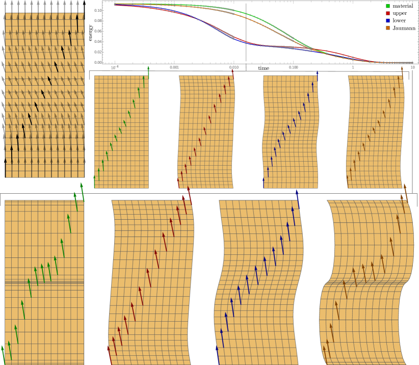
Figure 4: Solutions for the $\operatorname{L}^{\!2}$-gradient flows (58) with $K=0.1$ and $\omega=0.5$: The initial solution (top left) is periodic on the boundaries and constant horizontally. Vertically, it is counterclockwisely twisted and compressed towards the center. For a better readability, vector field solutions are only plotted on a diagonal without loss of information. The solutions are approximated for four different models, where we assume the gauge of surface independence and time derivative consistently, namely the material, upper-convected, lower-convected and Jaumann gauge/derivative (from left to right). All energy paths (top right) are decreasing as expected by energy rate (40) with $\boldsymbol{\Phi}=\boldsymbol{\Psi}$. The energy plot has a log-scale on its time axis. Vector field solutions tend to be parallel aligned with a constant length towards the time process. We show the solution at time $t=0.016$ (middle row) and $t=10$ (bottom row), where the solutions almost reached their minimal state. The time-step width $\tau$ of the time discretization increase step-wise from $\tau=10^{-4}$ at the beginning until $\tau=0.45$ at the end, see the semitransparent gray dots at the energy paths. The grid width $h=10^{-2}$ is constant along the vertical local Lagrange coordinate $y^{2}$ for all times. The horizontal gray gridlines only represent every fourth available spatial line, i. e., the distance between two gridlines is $0.04$ constantly on local Lagrange coordinates. Solutions are plotted w. r. t. Euler coordinates, i. e., w. r. t. the embedding space, to show the local deformations of the underlying domain towards the minimum state. Any impressions that the surface gets bent in normal direction is just an optical illusion. In absence of normal forces the surface stays flat all times. (Video online: mendeley_video )

The highly nonlinear equations (58) is discretized by an implicit Euler scheme in time, where we linearize all terms by one step Taylor expansion at the old time step. We use FDM with central differential quotients for any order of spatial derivatives. Solving the resulting discrete linear system is done with the UMFPACK library in every time step. Unfortunately, it was only possible to get stable solutions for a consistent choice of gauge and time derivative with this proceeding. Therefore, the energy rate (40) becomes $\frac{d}{dt}\mathfrak{U}=-\lambda\left\|\nabla_{\operatorname{L}^{\!2}}\mathfrak{U}\right\|_{\operatorname{L}^{\!2}(\tensor{\operatorname{T}\!}{}\mathbb{R}^{3}|_{\mathcal{S}}\times\tensor{\operatorname{T}\!}{}\mathcal{S})}^{2}\leq 0$, i. e., the analytical solutions guarantee dissipation. This is also reflected by the numerical solutions, see figure 4.

4.3 Minimizing Landau-de Gennes-Helfrich Energy

A $\operatorname{L}^{\!2}$-gradient flow is given in Reuteretal_PRSA_2020 for the Landau-de Gennes-Helfrich energy, where $\boldsymbol{q}[\boldsymbol{X}]\in\mathcal{Q}^{2}\mathcal{S}<\tensor{\operatorname{T}\!}{{}^{2}}\mathcal{S}$ is a trace-free and symmetric 2-tensor field and surface deformations are restricted to deformations in normals direction. The resulting equations of motion are formulated under the material gauge of surface independence and with the material time derivative. The calculated energy rate also fits the energy rate (50) for the given restrictions.

5 Conclusions

Tangential tensor fields are usually defined at their underlying surface. However, if the surface smoothly changes, the field has to be also defined on the deformed surface, e. g., through various pushforwards. The linear change of these definitions is quantified by so-called deformation derivatives and can be seen as local domain variations of first kind of the fields. Similarly to time derivatives, deformation derivatives can be defined in different ways. We presented one for scalar fields, four for tangential vector fields and six for tangential 2-tensor fields. With these deformation derivatives we can quantify what it means for a tensor field to be independent of the underlying surface, which leads to the different definitions of the gauges of surface independence, where deformation derivatives vanish for all possible deformations of the surface. For non-scalar fields further possibilities exist to define deformation derivatives and thus gauges of surface independence. However, those chosen already cover a wide range of physically meaningful applications. Moreover, we disregard to handle $n$-tensor fields for $n>2$ for reasons of space. It does not bear any difficulties to do it for fixed $n$ in the same way as for $n=1,2$, though it becomes quit technical for general tensor orders. Also an extension to $d$-dimensional hyper-surfaces smoothly embedded in a higher dimensional Euclidean space, with co-dimension greater than one, should not pose a major challenge.

We see the primary application for the gauges of surface independence in the derivation of $\operatorname{L}^{\!2}$-gradient flows of energies, where the phase space comprises the surface itself among tensor quantities defined on it. In order to guarantee a decreasing energy in the $\operatorname{L}^{\!2}$-gradient flow the time derivative and the gauge of surface independence have to be chosen consistently. The choice should thereby follow physical arguments. We suggest to imagine how the considered tensor field would act under force-free transport and select a time derivative and a gauge of surface independence which fits the expected physical behavior, see e. g., Nitschke_2022 . Another possibility is to contemplate on a physically suitable pushforward for the tensor field, since its linear information determine a gauge of surface independence. Both provide a systematic way to select an appropriate $\operatorname{L}^{\!2}$-gradient flow.

Note that equilibrium states, stable or not, are independent on the choice of the gauge of surface independence, see discussion above (37). But in many situations these states are not unique. Therefore, steepest decent methods, like the $\operatorname{L}^{\!2}$-gradient flow, which approach the equilibrium state from non-equilibrium states, can give quit different results for different gauges of surface independence. This dependence on the gauge of surface independence has been shown by an example in section 4.2.

Besides these physical implications this work gives also some helpful tools for variations of first kind. Identity (33), and its special case (32), allow to variate under a specific gauge of surface independence, though the tensor field actually obeys a different gauge. We used this for the example in section 4.2 to circumvent calculating all commutators w. r. t. the covariant spatial and deformation derivative. Instead we could derive the variation only for a single gauge, which seems to simplify the situation, and concluded on the general case afterwards. We like to mention that the total variation $\frac{\operatorname{\delta}\!\mathfrak{U}}{\operatorname{\delta}\!\boldsymbol{X}}$, deformation derivatives, and hence also the gauges, following a general principle of covariance, i. e., they are independent of their syntactical description, e. g., partial dependencies in $\mathfrak{U}$ or coordinates dependencies. Contrarily, the strong formulation of the $\operatorname{L}^{\!2}$-gradient (36), in terms of partial variation and gauge stress, is certainly helpful, but both summands have to be interpreted in the context of the syntax of $\mathfrak{U}$. We showed in Appendix A.1 and A.2, that this has no influence on the left-hand side of (36).

Acknowledgments

AV was supported by DFG through FOR3013.

Appendix A Alternative Proceedings

A.1 Contravariant Proxy Approach to (32)

Instead of considering tangential vector fields $\boldsymbol{q}[\boldsymbol{X}]\in\tensor{\operatorname{T}\!}{}\mathcal{S}$ together with an associated frame, some readers may prefer to use the contravariant proxy field $\{q^{i}[\boldsymbol{X}]\}\in(\tensor{\operatorname{T}\!}{{}^{0}}\mathcal{S})^{2}$, where in case of an embedding with parameterization $\boldsymbol{X}$ holds $q^{i}[\boldsymbol{X}]\partial_{i}\boldsymbol{X}=\boldsymbol{q}[\boldsymbol{X}]$, resp. $q^{i}[\boldsymbol{X}]=g^{ij}[\boldsymbol{X}]\left\langle\boldsymbol{q}[\boldsymbol{X}],\partial_{j}\boldsymbol{X}\right\rangle_{\tensor{\operatorname{T}\!}{}\mathcal{S}}$. Therefore, we can rewrite the energy $\mathfrak{U}$ in section 3.2.2 by

$$\widetilde{\mathfrak{U}}[\boldsymbol{X},q^{1}[\boldsymbol{X}],q^{2}[\boldsymbol{X}]] :=\mathfrak{U}[\boldsymbol{X},\boldsymbol{q}[\boldsymbol{X}]]$$ (59)

without changing the sematic of $\mathcal{U}$. The great advantage of total derivations, such as the total variation (27), is that they are syntactical invariant, i. e., the total variation

$$\left\langle\frac{\operatorname{\delta}\!\widetilde{\mathfrak{U}}}{\operatorname{\delta}\!\boldsymbol{X}},\boldsymbol{W}\right\rangle :=\lim_{\varepsilon\rightarrow 0}\frac{\widetilde{\mathfrak{U}}[\boldsymbol{X}+\varepsilon\boldsymbol{W},q^{1}[\boldsymbol{X}+\varepsilon\boldsymbol{W}],q^{2}[\boldsymbol{X}+\varepsilon\boldsymbol{W}]]-\widetilde{\mathfrak{U}}[\boldsymbol{X},q^{1}[\boldsymbol{X}],q^{2}[\boldsymbol{X}]]}{\varepsilon}$$

in an arbitrary direction $\boldsymbol{W}\in\tensor{\operatorname{T}\!}{}\mathbb{R}^{3}|_{\mathcal{S}}$ equals $\left\langle\frac{\operatorname{\delta}\!\mathfrak{U}}{\operatorname{\delta}\!\boldsymbol{X}},\boldsymbol{W}\right\rangle$ (27) as we can easily see by substitution (59). The total variations w. r. t. contravariant proxy components in direction of arbitrary scalar fields $f\in\tensor{\operatorname{T}\!}{{}^{0}}\mathcal{S}$ are

$$\left\langle\frac{\operatorname{\delta}\!\widetilde{\mathfrak{U}}}{\operatorname{\delta}\!q^{1}},f\right\rangle :=\lim_{\varepsilon\rightarrow 0}\frac{\widetilde{\mathfrak{U}}[\boldsymbol{X},q^{1}[\boldsymbol{X}]+\varepsilon f,q^{2}[\boldsymbol{X}]]-\widetilde{\mathfrak{U}}[\boldsymbol{X},q^{1}[\boldsymbol{X}],q^{2}[\boldsymbol{X}]]}{\varepsilon}\,\text{,}$$

$$\left\langle\frac{\operatorname{\delta}\!\widetilde{\mathfrak{U}}}{\operatorname{\delta}\!q^{2}},f\right\rangle :=\lim_{\varepsilon\rightarrow 0}\frac{\widetilde{\mathfrak{U}}[\boldsymbol{X},q^{1}[\boldsymbol{X}],q^{2}[\boldsymbol{X}]+\varepsilon f]-\widetilde{\mathfrak{U}}[\boldsymbol{X},q^{1}[\boldsymbol{X}],q^{2}[\boldsymbol{X}]]}{\varepsilon}\,\text{.}$$

Since $\mathfrak{U}[\boldsymbol{X},\boldsymbol{q}[\boldsymbol{X}]+\varepsilon\boldsymbol{r}]=\widetilde{\mathfrak{U}}[\boldsymbol{X},q^{1}[\boldsymbol{X}]+\varepsilon r^{1},q^{2}[\boldsymbol{X}]+\varepsilon r^{2}]$ is valid for an arbitrary tangential field $\boldsymbol{r}=r^{i}\partial_{i}\boldsymbol{X}\in\tensor{\operatorname{T}\!}{}\mathcal{S}$, the relation to the total variation (28) is

$$\left\langle\frac{\operatorname{\delta}\!\mathfrak{U}}{\operatorname{\delta}\!\boldsymbol{q}},\boldsymbol{r}\right\rangle =\left\langle\frac{\operatorname{\delta}\!\widetilde{\mathfrak{U}}}{\operatorname{\delta}\!q^{1}},r^{1}\right\rangle+\left\langle\frac{\operatorname{\delta}\!\widetilde{\mathfrak{U}}}{\operatorname{\delta}\!q^{2}},r^{2}\right\rangle=\left\langle\frac{\operatorname{\delta}\!\widetilde{\mathfrak{U}}}{\operatorname{\delta}\!q^{i}},r^{i}\right\rangle\,\text{.}$$

To get a decomposition as (32) to separate determined and not determined parts, the proceeding is almost the same. We use a Taylor expansion with a reasonable pushforward for scalar fields, i. e., it holds

$$q^{i}[\boldsymbol{X}+\varepsilon\boldsymbol{W}] =(q^{i}[\boldsymbol{X}])^{*_{\varepsilon\boldsymbol{W}}}+\varepsilon(\tensor*{\eth}{{}_{\boldsymbol{W}}}q^{i}[\boldsymbol{X}])^{*_{\varepsilon\boldsymbol{W}}}+\mathcal{O}(\varepsilon^{2})$$

$$\forall f\in\tensor{\operatorname{T}\!}{{}^{0}}\mathcal{S}:\quad f^{*_{\varepsilon\boldsymbol{W}}}(y^{1},y^{2}) :=f(y^{1},y^{2})\in\tensor*{\operatorname{T}\!}{{}^{0}_{(\boldsymbol{X}+\varepsilon\boldsymbol{W})(y^{1},y^{2})}}\mathcal{S}_{\varepsilon\boldsymbol{W}}$$ (60)

with scalar-valued deformation derivative $\tensor*{\eth}{{}_{\boldsymbol{W}}}:\tensor{\operatorname{T}\!}{{}^{0}}\mathcal{S}\rightarrow\tensor{\operatorname{T}\!}{{}^{0}}\mathcal{S}$ (17). Another Taylor expansion and exploiting the vector space structure of an consistently chosen Hilbert space gives

$$\widetilde{\mathfrak{U}}[\boldsymbol{X}+\varepsilon\boldsymbol{W},q^{1}[\boldsymbol{X}+\varepsilon\boldsymbol{W}],q^{2}[\boldsymbol{X}+\varepsilon\boldsymbol{W}]]$$

$$=\widetilde{\mathfrak{U}}[\boldsymbol{X}+\varepsilon\boldsymbol{W},(q^{1}[\boldsymbol{X}])^{*_{\varepsilon\boldsymbol{W}}},(q^{2}[\boldsymbol{X}])^{*_{\varepsilon\boldsymbol{W}}}]$$

$$\quad+\varepsilon\left\langle\frac{\operatorname{\delta}\!\widetilde{\mathfrak{U}}}{\operatorname{\delta}\!(q^{i})^{*_{\varepsilon\boldsymbol{W}}}},(\tensor*{\eth}{{}_{\boldsymbol{W}}}q^{i}[\boldsymbol{X}])^{*_{\varepsilon\boldsymbol{W}}}\right\rangle_{\operatorname{L}^{\!2}(\tensor{\operatorname{T}\!}{{}^{0}}\mathcal{S}_{\varepsilon\boldsymbol{W}})}+\mathcal{O}(\varepsilon^{2})\,\text{.}$$

Since $*_{\varepsilon\boldsymbol{W}}\rightarrow\operatorname{Id}_{\tensor{\operatorname{T}\!}{{}^{0}}\mathcal{S}}$ is valid for $\varepsilon\rightarrow 0$, we obtain the total variation

$$\left\langle\frac{\operatorname{\delta}\!\widetilde{\mathfrak{U}}}{\operatorname{\delta}\!\boldsymbol{X}},\boldsymbol{W}\right\rangle_{\operatorname{L}^{\!2}(\tensor{\operatorname{T}\!}{}\mathbb{R}^{3}|_{\mathcal{S}})} =\left\langle\frac{\partial\widetilde{\mathfrak{U}}}{\partial\boldsymbol{X}},\boldsymbol{W}\right\rangle_{\operatorname{L}^{\!2}(\tensor{\operatorname{T}\!}{}\mathbb{R}^{3}|_{\mathcal{S}})}+\left\langle\frac{\operatorname{\delta}\!\widetilde{\mathfrak{U}}}{\operatorname{\delta}\!q^{i}},\tensor*{\eth}{{}_{\boldsymbol{W}}}q^{i}[\boldsymbol{X}]\right\rangle_{\operatorname{L}^{\!2}(\tensor{\operatorname{T}\!}{{}^{0}}\mathcal{S})}$$ (61)

by defining the partial variation

$$\left\langle\frac{\partial\widetilde{\mathfrak{U}}}{\partial\boldsymbol{X}},\boldsymbol{W}\right\rangle :=\lim_{\varepsilon\rightarrow 0}\frac{\widetilde{\mathfrak{U}}[\boldsymbol{X}+\varepsilon\boldsymbol{W},(q^{1}[\boldsymbol{X}])^{*_{\varepsilon\boldsymbol{W}}},(q^{2}[\boldsymbol{X}])^{*_{\varepsilon\boldsymbol{W}}}]-\widetilde{\mathfrak{U}}[\boldsymbol{X},q^{1}[\boldsymbol{X}],q^{2}[\boldsymbol{X}]]}{\varepsilon}\,\text{.}$$

In praxis this means to differentiate everything of the energy w. r. t. $\boldsymbol{X}$ except contravariant proxy components of $\boldsymbol{q}[\boldsymbol{X}]$, e. g., in the term $\int_{\mathcal{S}}\|\boldsymbol{q}[\boldsymbol{X}]\|^{2}\mu[\boldsymbol{X}]=\int_{\mathcal{S}}g_{ij}[\boldsymbol{X}]q^{i}[\boldsymbol{X}]q^{j}[\boldsymbol{X}]\mu[\boldsymbol{X}]$ has only $g_{ij}[\boldsymbol{X}]$ and $\mu[\boldsymbol{X}]$ to be differentiated. Moreover, comparing with (32) reveals

$$\left\langle\frac{\partial\widetilde{\mathfrak{U}}}{\partial\boldsymbol{X}},\boldsymbol{W}\right\rangle_{\operatorname{L}^{\!2}(\tensor{\operatorname{T}\!}{}\mathbb{R}^{3}|_{\mathcal{S}})} =\left\langle\frac{\partial\mathfrak{U}}{\partial\boldsymbol{X}},\boldsymbol{W}\right\rangle_{\operatorname{L}^{\!2}(\tensor{\operatorname{T}\!}{}\mathbb{R}^{3}|_{\mathcal{S}})}+\left\langle\frac{\operatorname{\delta}\!\mathfrak{U}}{\operatorname{\delta}\!\boldsymbol{q}},\boldsymbol{G}[\boldsymbol{X},\boldsymbol{W}]\boldsymbol{q}[\boldsymbol{X}]\right\rangle_{\operatorname{L}^{\!2}(\tensor{\operatorname{T}\!}{}\mathcal{S})}\,\text{,}$$

$$\left\langle\frac{\operatorname{\delta}\!\widetilde{\mathfrak{U}}}{\operatorname{\delta}\!q^{i}},\tensor*{\eth}{{}_{\boldsymbol{W}}}q^{i}[\boldsymbol{X}]\right\rangle_{\operatorname{L}^{\!2}(\tensor{\operatorname{T}\!}{{}^{0}}\mathcal{S})} =\left\langle\frac{\operatorname{\delta}\!\mathfrak{U}}{\operatorname{\delta}\!\boldsymbol{q}},\tensor*{\eth}{{}_{\boldsymbol{W}}^{\sharp}}\boldsymbol{q}[\boldsymbol{X}]\right\rangle_{\operatorname{L}^{\!2}(\tensor{\operatorname{T}\!}{}\mathcal{S})}$$

$$=\left\langle\frac{\operatorname{\delta}\!\mathfrak{U}}{\operatorname{\delta}\!\boldsymbol{q}},\tensor*{\eth}{{}_{\boldsymbol{W}}^{\mathcal{S}}}\boldsymbol{q}[\boldsymbol{X}]-\boldsymbol{G}[\boldsymbol{X},\boldsymbol{W}]\boldsymbol{q}[\boldsymbol{X}]\right\rangle_{\operatorname{L}^{\!2}(\tensor{\operatorname{T}\!}{}\mathcal{S})}\,\text{.}$$

This also affects the $\operatorname{L}^{\!2}$-gradient (36) in section 3.2.4, which becomes

$$\nabla_{\operatorname{L}^{\!2}}\widetilde{\mathfrak{U}} =\left(\frac{\operatorname{\delta}\!\widetilde{\mathfrak{U}}}{\operatorname{\delta}\!\boldsymbol{X}},\left\{\frac{\operatorname{\delta}\!\widetilde{\mathfrak{U}}}{\operatorname{\delta}\!q^{i}}\right\}\right)=\left(\frac{\partial\widetilde{\mathfrak{U}}}{\partial\boldsymbol{X}}-\operatorname{div}_{\tensor{\operatorname{T}\!}{{}^{2}}\mathcal{S}}\widetilde{\boldsymbol{\sigma}},\left\{\frac{\operatorname{\delta}\!\widetilde{\mathfrak{U}}}{\operatorname{\delta}\!q^{i}}\right\}\right)\,\text{,}$$ (62)

where $\widetilde{\boldsymbol{\sigma}}=\boldsymbol{\sigma}-\frac{\operatorname{\delta}\!\mathfrak{U}}{\operatorname{\delta}\!\boldsymbol{q}}\otimes\boldsymbol{q}[\boldsymbol{X}]\in\tensor{\operatorname{T}\!}{{}^{2}}\mathcal{S}$ is given in table 3 depending on the chosen gauge.

A.2 Approach to (32) with explicit covariant metric proxy

Some readers would like to include the covariant metric proxy $\{g_{ij}[\boldsymbol{X}]\}=\{\left\langle\partial_{i}\boldsymbol{X},\partial_{j}\boldsymbol{X}\right\rangle_{\tensor{\operatorname{T}\!}{}\mathbb{R}^{3}|_{\mathcal{S}}}\}\in(\tensor{\operatorname{T}\!}{{}^{0}}\mathcal{S})^{2\times 2}$, so that the energy $\mathfrak{U}$ can be rewritten as

$$\widehat{\mathfrak{U}}[\boldsymbol{X},\boldsymbol{q}[\boldsymbol{X}],\{g_{ij}[\boldsymbol{X}]\}] :=\mathfrak{U}[\boldsymbol{X},\boldsymbol{q}[\boldsymbol{X}]]$$

without changing the sematic of $\mathcal{U}$. The total variation

$$\left\langle\frac{\operatorname{\delta}\!\widehat{\mathfrak{U}}}{\operatorname{\delta}\!\boldsymbol{X}},\boldsymbol{W}\right\rangle :=\lim_{\varepsilon\rightarrow 0}\frac{\widehat{\mathfrak{U}}[\boldsymbol{X}+\varepsilon\boldsymbol{W},\boldsymbol{q}[\boldsymbol{X}+\varepsilon\boldsymbol{W}],\{g_{ij}[\boldsymbol{X}]+\varepsilon\boldsymbol{W}\}]-\widehat{\mathfrak{U}}[\boldsymbol{X},\boldsymbol{q}[\boldsymbol{X}],\{g_{ij}[\boldsymbol{X}]\}]}{\varepsilon}$$

w. r. t. $\boldsymbol{X}$ in arbitrary directions of $\boldsymbol{W}\in\tensor{\operatorname{T}\!}{}\mathbb{R}^{3}|_{\mathcal{S}}$ equals $\left\langle\frac{\operatorname{\delta}\!\mathfrak{U}}{\operatorname{\delta}\!\boldsymbol{X}},\boldsymbol{W}\right\rangle$ (27) as expected for a total derivative. Also the total variation

$$\left\langle\frac{\operatorname{\delta}\!\widehat{\mathfrak{U}}}{\operatorname{\delta}\!\boldsymbol{q}},\boldsymbol{r}\right\rangle :=\lim_{\varepsilon\rightarrow 0}\frac{\widehat{\mathfrak{U}}[\boldsymbol{X},\boldsymbol{q}[\boldsymbol{X}]+\varepsilon\boldsymbol{r},\{g_{ij}[\boldsymbol{X}]\}]-\widehat{\mathfrak{U}}[\boldsymbol{X},\boldsymbol{q}[\boldsymbol{X}],\{g_{ij}[\boldsymbol{X}]\}]}{\varepsilon}$$

w. r. t. $\boldsymbol{q}[\boldsymbol{X}]$ in arbitrary directions of $\boldsymbol{r}\in\tensor{\operatorname{T}\!}{}\mathcal{S}$ equals $\left\langle\frac{\operatorname{\delta}\!\mathfrak{U}}{\operatorname{\delta}\!\boldsymbol{q}},\boldsymbol{r}\right\rangle$ (28). The Taylor expansion

$$g_{ij}[\boldsymbol{X}+\varepsilon\boldsymbol{W}] =(g_{ij}[\boldsymbol{X}])^{*_{\varepsilon\boldsymbol{W}}}+\varepsilon(S_{ij}[\boldsymbol{X},\boldsymbol{W}])^{*_{\varepsilon\boldsymbol{W}}}+\mathcal{O}(\varepsilon^{2})$$

with scalar-valued pushforward $*_{\varepsilon\boldsymbol{W}}:\tensor{\operatorname{T}\!}{{}^{0}}\mathcal{S}\rightarrow\tensor{\operatorname{T}\!}{{}^{0}}\mathcal{S}_{\varepsilon\boldsymbol{W}}$ (60) yields

$$\widehat{\mathfrak{U}}[\boldsymbol{X}+\varepsilon\boldsymbol{W},\boldsymbol{q}[\boldsymbol{X}+\varepsilon\boldsymbol{W}],\{g_{ij}[\boldsymbol{X}+\varepsilon\boldsymbol{W}]\}]$$

$$=\widehat{\mathfrak{U}}[\boldsymbol{X}+\varepsilon\boldsymbol{W},\operatorname{\Pi}_{\tensor{\operatorname{T}\!}{}\mathcal{S}_{\varepsilon\boldsymbol{W}}}\left(\boldsymbol{q}[\boldsymbol{X}]\right)^{*_{\varepsilon\boldsymbol{W}}},\{(g_{ij}[\boldsymbol{X}])^{*_{\varepsilon\boldsymbol{W}}}\}]$$

$$\quad\quad+\varepsilon\left\langle\frac{\operatorname{\delta}\!\widehat{\mathfrak{U}}}{\operatorname{\delta}\!(\operatorname{\Pi}_{\tensor{\operatorname{T}\!}{}\mathcal{S}_{\varepsilon\boldsymbol{W}}}\boldsymbol{q}^{*_{\varepsilon\boldsymbol{W}}})},\operatorname{\Pi}_{\tensor{\operatorname{T}\!}{}\mathcal{S}_{\varepsilon\boldsymbol{W}}}\left(\tensor*{\eth}{{}_{\boldsymbol{W}}}\boldsymbol{q}[\boldsymbol{X}]\right)^{*_{\varepsilon\boldsymbol{W}}}\right\rangle_{\operatorname{L}^{\!2}(\tensor{\operatorname{T}\!}{}\mathcal{S}_{\varepsilon\boldsymbol{W}})}$$

$$\quad\quad+\varepsilon\left\langle\frac{\partial\widehat{\mathfrak{U}}}{\partial g_{ij}^{*_{\varepsilon\boldsymbol{W}}}},(S_{ij}[\boldsymbol{X},\boldsymbol{W}])^{*_{\varepsilon\boldsymbol{W}}}\right\rangle_{\operatorname{L}^{\!2}(\tensor{\operatorname{T}\!}{{}^{0}}\mathcal{S}_{\varepsilon\boldsymbol{W}})}+\mathcal{O}(\varepsilon^{2})\,\text{,}$$

where $*_{\varepsilon\boldsymbol{W}}$ on vector fields applies $\mathbb{R}^{3}$-component-wise, see (29). For partial variations w. r. t. metric components see (64) below, but on $\mathcal{S}_{\varepsilon\boldsymbol{W}}$ instead. Since $*_{\varepsilon\boldsymbol{W}}\rightarrow\operatorname{Id}$ on their respective spaces and $\operatorname{\Pi}_{\tensor{\operatorname{T}\!}{}\mathcal{S}_{\varepsilon\boldsymbol{W}}}\rightarrow\operatorname{\Pi}_{\tensor{\operatorname{T}\!}{}\mathcal{S}}$ for $\varepsilon\rightarrow 0$, we obtain

$$\left\langle\frac{\operatorname{\delta}\!\widehat{\mathfrak{U}}}{\operatorname{\delta}\!\boldsymbol{X}},\boldsymbol{W}\right\rangle_{\operatorname{L}^{\!2}(\tensor{\operatorname{T}\!}{}\mathbb{R}^{3}|_{\mathcal{S}})} =\left\langle\frac{\partial\widehat{\mathfrak{U}}}{\partial\boldsymbol{X}},\boldsymbol{W}\right\rangle_{\operatorname{L}^{\!2}(\tensor{\operatorname{T}\!}{}\mathbb{R}^{3}|_{\mathcal{S}})}+\left\langle\frac{\operatorname{\delta}\!\widehat{\mathfrak{U}}}{\operatorname{\delta}\!\boldsymbol{q}},\tensor*{\eth}{{}_{\boldsymbol{W}}^{\mathcal{S}}}\boldsymbol{q}[\boldsymbol{X}]\right\rangle_{\operatorname{L}^{\!2}(\tensor{\operatorname{T}\!}{}\mathcal{S})}$$

$$\quad\quad+\left\langle\frac{\partial\widehat{\mathfrak{U}}}{\partial g_{ij}},S_{ij}[\boldsymbol{X},\boldsymbol{W}]\right\rangle_{\operatorname{L}^{\!2}(\tensor{\operatorname{T}\!}{{}^{0}}\mathcal{S})}\,\text{,}$$ (63)

where the partial variations w. r. t. covariant metric proxy components in direction of scalar fields $f\in\tensor{\operatorname{T}\!}{}\mathcal{S}$ are defined by

$$\left\langle\frac{\partial\widehat{\mathfrak{U}}}{\partial g_{ij}},f\right\rangle :=\lim_{\varepsilon\rightarrow 0}\frac{\widehat{\mathfrak{U}}[\boldsymbol{X},\boldsymbol{q}[\boldsymbol{X}],\{g_{ij}[\boldsymbol{X}]+\varepsilon f\}]-\widehat{\mathfrak{U}}[\boldsymbol{X},\boldsymbol{q}[\boldsymbol{X}],\{g_{ij}[\boldsymbol{X}]\}]}{\varepsilon}$$ (64)

and the partial variation w. r. t.$\boldsymbol{X}$ in directions of $\boldsymbol{W}\in\tensor{\operatorname{T}\!}{}\mathbb{R}^{3}|_{\mathcal{S}}$ by

$$\left\langle\frac{\partial\widehat{\mathfrak{U}}}{\partial\boldsymbol{X}},\boldsymbol{W}\right\rangle:=\lim_{\varepsilon\rightarrow 0}\frac{1}{\varepsilon}\Big{(} \widehat{\mathfrak{U}}[\boldsymbol{X}+\varepsilon\boldsymbol{W},\operatorname{\Pi}_{\tensor{\operatorname{T}\!}{}\mathcal{S}_{\varepsilon\boldsymbol{W}}}\left(\boldsymbol{q}[\boldsymbol{X}]\right)^{*_{\varepsilon\boldsymbol{W}}},\{(g_{ij}[\boldsymbol{X}])^{*_{\varepsilon\boldsymbol{W}}}\}]$$

$$-\widehat{\mathfrak{U}}[\boldsymbol{X},\boldsymbol{q}[\boldsymbol{X}],\{g_{ij}[\boldsymbol{X}]\}]\Big{)}\,\text{.}$$

In praxis this means to differentiate everything of the energy w. r. t. $\boldsymbol{X}$ except for $\boldsymbol{q}[\boldsymbol{X}]$ (incl. its frame) and explicit terms of $g_{ij}[\boldsymbol{X}]$, e. g., in the term $\int_{\mathcal{S}}\|\boldsymbol{q}[\boldsymbol{X}]\|^{2}\mu[\boldsymbol{X}]=\int_{\mathcal{S}}\|\boldsymbol{q}[\boldsymbol{X}]\|^{2}\widehat{\mu}[\{g_{ij}[\boldsymbol{X}]\}]$ nothing has to be differentiated, i. e., $\left\langle\frac{\partial\widehat{\mathfrak{U}}}{\partial\boldsymbol{X}},\boldsymbol{W}\right\rangle=0$. Moreover, comparing with (32) reveals

$$\left\langle\frac{\partial\widehat{\mathfrak{U}}}{\partial\boldsymbol{X}},\boldsymbol{W}\right\rangle_{\operatorname{L}^{\!2}(\tensor{\operatorname{T}\!}{}\mathbb{R}^{3}|_{\mathcal{S}})}+\left\langle\frac{\partial\widehat{\mathfrak{U}}}{\partial g_{ij}},S_{ij}[\boldsymbol{X},\boldsymbol{W}]\right\rangle_{\operatorname{L}^{\!2}(\tensor{\operatorname{T}\!}{{}^{0}}\mathcal{S})} =\left\langle\frac{\partial\mathfrak{U}}{\partial\boldsymbol{X}},\boldsymbol{W}\right\rangle_{\operatorname{L}^{\!2}(\tensor{\operatorname{T}\!}{}\mathbb{R}^{3}|_{\mathcal{S}})}$$

and $\left\langle\frac{\operatorname{\delta}\!\widehat{\mathfrak{U}}}{\operatorname{\delta}\!\boldsymbol{q}},\tensor*{\eth}{{}_{\boldsymbol{W}}^{\mathcal{S}}}\boldsymbol{q}[\boldsymbol{X}]\right\rangle_{\operatorname{L}^{\!2}(\tensor{\operatorname{T}\!}{}\mathcal{S})}=\left\langle\frac{\operatorname{\delta}\!\mathfrak{U}}{\operatorname{\delta}\!\boldsymbol{q}},\tensor*{\eth}{{}_{\boldsymbol{W}}^{\mathcal{S}}}\boldsymbol{q}[\boldsymbol{X}]\right\rangle_{\operatorname{L}^{\!2}(\tensor{\operatorname{T}\!}{}\mathcal{S})}$ as expected for a total derivative w. r. t. same arguments. Note that we could substitute $\left\langle\frac{\partial\widehat{\mathfrak{U}}}{\partial g_{ij}},S_{ij}[\boldsymbol{X},\boldsymbol{W}]\right\rangle_{\operatorname{L}^{\!2}(\tensor{\operatorname{T}\!}{{}^{0}}\mathcal{S})}=\left\langle\frac{\partial\widehat{\mathfrak{U}}}{\partial g_{ij}},G_{ij}[\boldsymbol{X},\boldsymbol{W}]\right\rangle_{\operatorname{L}^{\!2}(\tensor{\operatorname{T}\!}{{}^{0}}\mathcal{S})}$ due to symmetry.

Appendix B Outsourced Calculations

B.1 Deformation Derivative on Geometrical Quantities

B.1.1 Metric Tensor, its Inverse and Density

With the metric tensor proxy, given by $g_{ij}[\boldsymbol{X}]=\left\langle\partial_{i}\boldsymbol{X},\partial_{j}\boldsymbol{X}\right\rangle_{\tensor{\operatorname{T}\!}{}\mathbb{R}^{3}|_{\mathcal{S}}}$, contravariant proxy components $G_{ij}[\boldsymbol{X},\boldsymbol{W}]$ (10) of the tangential derivative of deformation direction $\boldsymbol{W}\in\tensor{\operatorname{T}\!}{}\mathbb{R}^{3}|_{\mathcal{S}}$ and the symmetric part $S_{ij}[\boldsymbol{X},\boldsymbol{W}]$, the deformation derivative (17) on scalar fields yields

$$\tensor*{\eth}{{}_{\boldsymbol{W}}}g_{ij}[\boldsymbol{X}] =\left\langle\partial_{i}\boldsymbol{W},\partial_{j}\boldsymbol{X}\right\rangle_{\tensor{\operatorname{T}\!}{}\mathbb{R}^{3}|_{\mathcal{S}}}+\left\langle\partial_{i}\boldsymbol{X},\partial_{j}\boldsymbol{W}\right\rangle_{\tensor{\operatorname{T}\!}{}\mathbb{R}^{3}|_{\mathcal{S}}}=G_{ij}[\boldsymbol{X},\boldsymbol{W}]+G_{ji}[\boldsymbol{X},\boldsymbol{W}]$$

$$=2S_{ij}[\boldsymbol{X},\boldsymbol{W}]\,\text{.}$$ (65)

Due to this, the inverse tensor proxy gives

$$\tensor*{\eth}{{}_{\boldsymbol{W}}}g^{ij}[\boldsymbol{X}] =\tensor*{\eth}{{}_{\boldsymbol{W}}}\left(g^{ik}[\boldsymbol{X}]g^{jl}[\boldsymbol{X}]g_{kl}[\boldsymbol{X}]\right)=2\tensor*{\eth}{{}_{\boldsymbol{W}}}g^{ij}[\boldsymbol{X}]+2S^{ij}[\boldsymbol{X},\boldsymbol{W}]$$

$$=-2S^{ij}[\boldsymbol{X},\boldsymbol{W}]$$ (66)

and the density value $\sqrt{|\boldsymbol{g}|}[\boldsymbol{X}]:=\sqrt{\det\boldsymbol{q}[\boldsymbol{X}]}\in\tensor{\operatorname{T}\!}{{}^{0}}\mathcal{S}$ yields

$$\tensor*{\eth}{{}_{\boldsymbol{W}}}\sqrt{|\boldsymbol{g}|}[\boldsymbol{X}] =\sqrt{|\boldsymbol{g}|}[\boldsymbol{X}]\operatorname{Tr}\boldsymbol{G}[\boldsymbol{X},\boldsymbol{W}]\,\text{,}$$

resp. $\tensor*{\eth}{{}_{\boldsymbol{W}}}\mu[\boldsymbol{X}]=\operatorname{Tr}\boldsymbol{G}[\boldsymbol{X},\boldsymbol{W}]\mu[\boldsymbol{X}]$, where $\mu[\boldsymbol{X}]=\sqrt{|\boldsymbol{g}|}[\boldsymbol{X}]dy^{1}\!\wedge\!dy^{2}\cong\boldsymbol{E}[\boldsymbol{X}]$.

B.1.2 Christoffel Symbols

With Christoffel symbols of first kind (5) and contravariant proxy components $G_{ij}[\boldsymbol{X},\boldsymbol{W}]$ (10) of the tangential derivative of deformation direction $\boldsymbol{W}\in\tensor{\operatorname{T}\!}{}\mathbb{R}^{3}|_{\mathcal{S}}$, the deformation derivative (17) on scalar fields yields

$$\tensor*{\eth}{{}_{\boldsymbol{W}}}\Gamma_{jkl}[\boldsymbol{X}] =\left\langle\partial_{j}\partial_{k}\boldsymbol{W},\partial_{l}\boldsymbol{X}\right\rangle_{\tensor{\operatorname{T}\!}{}\mathbb{R}^{3}|_{\mathcal{S}}}+\left\langle\partial_{j}\partial_{k}\boldsymbol{X},\partial_{l}\boldsymbol{W}\right\rangle_{\tensor{\operatorname{T}\!}{}\mathbb{R}^{3}|_{\mathcal{S}}}$$

$$=\partial_{j}G_{lk}[\boldsymbol{X},\boldsymbol{W}]-\left\langle\partial_{j}\partial_{l}\boldsymbol{X},\partial_{k}\boldsymbol{W}\right\rangle_{\tensor{\operatorname{T}\!}{}\mathbb{R}^{3}|_{\mathcal{S}}}+\left\langle\partial_{j}\partial_{k}\boldsymbol{X},\partial_{l}\boldsymbol{W}\right\rangle_{\tensor{\operatorname{T}\!}{}\mathbb{R}^{3}|_{\mathcal{S}}}$$

The full surface gradient $\nabla_{\mathcal{S}}\boldsymbol{W}=g^{il}(\partial_{l}\boldsymbol{W})\otimes\partial_{i}\boldsymbol{X}\in\tensor{\operatorname{T}\!}{}\mathbb{R}^{3}|_{\mathcal{S}}\otimes\tensor{\operatorname{T}\!}{}\mathcal{S}$ is given in (13), resp. (11) in components. The covariant Hessian components of $\boldsymbol{X}$ reads $\partial_{j}\partial_{k}\boldsymbol{X}=\Gamma_{jk}^{m}[\boldsymbol{X}]\partial_{m}\boldsymbol{X}+I\!I_{jk}[\boldsymbol{X}]\boldsymbol{\nu}[\boldsymbol{X}]$. Therefore, we obtain

$$\left\langle\partial_{j}\partial_{k}\boldsymbol{X},\partial_{l}\boldsymbol{W}\right\rangle_{\tensor{\operatorname{T}\!}{}\mathbb{R}^{3}|_{\mathcal{S}}} =\Gamma_{jk}^{m}[\boldsymbol{X}]G_{ml}[\boldsymbol{X},\boldsymbol{W}]+b_{l}[\boldsymbol{X},\boldsymbol{W}]I\!I_{jk}[\boldsymbol{X}]\,\text{,}$$

where $\boldsymbol{b}[\boldsymbol{X},\boldsymbol{W}]=\nabla w_{\bot}[\boldsymbol{X}]+\boldsymbol{I\!I}[\boldsymbol{X}]\boldsymbol{w}[\boldsymbol{X}]\in\tensor{\operatorname{T}\!}{}\mathcal{S}$ determines the normal-tangential part of $\nabla_{\mathcal{S}}\boldsymbol{W}$, see (14). Summing all things up and using the deformation of the inverse metric in (66), the deformation derivative of the Christoffel symbols of second kind yields

$$\tensor*{\eth}{{}_{\boldsymbol{W}}}\Gamma_{jk}^{i}[\boldsymbol{X}] =\tensor*{\eth}{{}_{\boldsymbol{W}}}\left(g^{il}[\boldsymbol{X}]\Gamma_{jkl}[\boldsymbol{X}]\right)=g^{il}\tensor*{\eth}{{}_{\boldsymbol{W}}}\Gamma_{jkl}[\boldsymbol{X}]-2S^{il}[\boldsymbol{X},\boldsymbol{W}]\Gamma_{jkl}[\boldsymbol{X}]$$

$$=\tensor{G}{{}^{i}_{k|j}}[\boldsymbol{X},\boldsymbol{W}]+b^{i}[\boldsymbol{X},\boldsymbol{W}]I\!I_{jk}[\boldsymbol{X}]-b_{k}[\boldsymbol{X},\boldsymbol{W}]I\!I^{i}_{j}[\boldsymbol{X}]\,\text{.}$$ (67)

B.1.3 Normals Field

The deformation derivative $\tensor*{\eth}{{}_{\boldsymbol{W}}}\boldsymbol{\nu}[\boldsymbol{X}]=(\tensor*{\eth}{{}_{\boldsymbol{W}}}\nu^{I}[\boldsymbol{X}])\boldsymbol{e}_{I}\in\tensor{\operatorname{T}\!}{}\mathcal{S}$ is tangential, since $\tensor*{\eth}{{}_{\boldsymbol{W}}}$ obeys the product rule w. r. t. the local inner product and the normals field $\boldsymbol{\nu}[\boldsymbol{X}]\in\tensor{\operatorname{T}\!}{}\mathbb{R}^{3}|_{\mathcal{S}}$ is normalized. Therefore, with (12) and (14), we can simply calculate

$$\tensor*{\eth}{{}_{\boldsymbol{W}}}\boldsymbol{\nu}[\boldsymbol{X}] =g^{ij}[\boldsymbol{X}]\left\langle\tensor*{\eth}{{}_{\boldsymbol{W}}}\boldsymbol{\nu}[\boldsymbol{X}],\partial_{j}\boldsymbol{X}\right\rangle_{\tensor{\operatorname{T}\!}{}\mathbb{R}^{3}|_{\mathcal{S}}}\partial_{i}\boldsymbol{X}=-g^{ij}[\boldsymbol{X}]\left\langle\boldsymbol{\nu}[\boldsymbol{X}],\partial_{j}\boldsymbol{W}\right\rangle_{\tensor{\operatorname{T}\!}{}\mathbb{R}^{3}|_{\mathcal{S}}}\partial_{i}\boldsymbol{X}$$

$$=-\left(\nabla w_{\bot}[\boldsymbol{X}]+\boldsymbol{I\!I}[\boldsymbol{X}]\boldsymbol{w}[\boldsymbol{X}]\right)=-\boldsymbol{b}[\boldsymbol{X},\boldsymbol{W}]\,\text{.}$$ (68)

B.1.4 Second Fundamental Form

With the deformation derivative (68) of the normal field and the normal part of the gradient of $\boldsymbol{W}$ in (12), the deformation derivative (17) of the covariant proxy components (3) of the second fundamental form yields

$$\tensor*{\eth}{{}_{\boldsymbol{W}}}I\!I_{ij}[\boldsymbol{X}] =\left\langle\partial_{j}\partial_{i}\boldsymbol{W},\boldsymbol{\nu}[\boldsymbol{X}]\right\rangle_{\tensor{\operatorname{T}\!}{}\mathbb{R}^{3}|_{\mathcal{S}}}-\left\langle\partial_{j}\partial_{i}\boldsymbol{X},\boldsymbol{b}[\boldsymbol{X},\boldsymbol{W}]\right\rangle_{\tensor{\operatorname{T}\!}{}\mathbb{R}^{3}|_{\mathcal{S}}}$$

$$=\partial_{j}\left\langle\partial_{i}\boldsymbol{W},\boldsymbol{\nu}[\boldsymbol{X}]\right\rangle_{\tensor{\operatorname{T}\!}{}\mathbb{R}^{3}|_{\mathcal{S}}}+\left\langle\partial_{i}\boldsymbol{W},I\!I^{k}_{j}[\boldsymbol{X}]\partial_{k}\boldsymbol{X}\right\rangle_{\tensor{\operatorname{T}\!}{}\mathbb{R}^{3}|_{\mathcal{S}}}-\Gamma_{ij}^{k}[\boldsymbol{X}]b_{k}[\boldsymbol{X},\boldsymbol{W}]$$

$$=b_{i|j}[\boldsymbol{X},\boldsymbol{W}]+G_{ki}[\boldsymbol{X},\boldsymbol{W}]I\!I^{k}_{j}[\boldsymbol{X}]=\left[\nabla\boldsymbol{b}[\boldsymbol{X},\boldsymbol{W}]+\boldsymbol{G}^{T}[\boldsymbol{X},\boldsymbol{W}]\boldsymbol{I\!I}[\boldsymbol{X}]\right]_{ij}\,\text{.}$$

Since $\left[\tensor*{\eth}{{}_{\boldsymbol{W}}^{\flat\flat}}\boldsymbol{I\!I}[\boldsymbol{X}]\right]_{ij}=\tensor*{\eth}{{}_{\boldsymbol{W}}}I\!I_{ij}[\boldsymbol{X}]$ is valid by (43), the relation (44) to the material deformation derivative (42) results in

$$\tensor*{\eth}{{}_{\boldsymbol{W}}^{\mathcal{S}}}\boldsymbol{I\!I}[\boldsymbol{X}] =\nabla\boldsymbol{b}[\boldsymbol{X},\boldsymbol{W}]-\boldsymbol{I\!I}[\boldsymbol{X}]\boldsymbol{G}[\boldsymbol{X},\boldsymbol{W}]\,\text{.}$$ (69)

B.2 Calculations for Example 4.2

The deformation derivative (67) of Christoffel symbols and the upper-lower deformation derivative in (43) yields

$$\tensor{\left[\tensor*{\eth}{{}_{\boldsymbol{W}}^{\sharp\flat}}\nabla\boldsymbol{q}[\boldsymbol{X}]\big{|}_{\tensor*{\eth}{{}^{\sharp}}\boldsymbol{q}=0}\right]}{{}^{i}_{k}} =\tensor*{\eth}{{}_{\boldsymbol{W}}}\tensor{q}{{}^{i}_{|k}}[\boldsymbol{X}]\big{|}_{\tensor*{\eth}{{}^{\sharp}}\boldsymbol{q}=0}=q^{j}[\boldsymbol{X}]\tensor*{\eth}{{}_{\boldsymbol{W}}}\Gamma_{kj}^{i}[\boldsymbol{X}]$$

$$=\big{[}\nabla_{\boldsymbol{q}[\boldsymbol{X}]}\boldsymbol{G}[\boldsymbol{X},\boldsymbol{W}]-\boldsymbol{I\!I}[\boldsymbol{X}]\boldsymbol{q}[\boldsymbol{X}]\otimes\boldsymbol{b}[\boldsymbol{X},\boldsymbol{W}]$$

$$\hskip 85.0pt+\boldsymbol{b}[\boldsymbol{X},\boldsymbol{W}]\otimes\boldsymbol{I\!I}[\boldsymbol{X}]\boldsymbol{q}[\boldsymbol{X}]\tensor{\big{]}}{{}^{i}_{k}}\,\text{,}$$

since $\tensor*{\eth}{{}_{\boldsymbol{W}}}\partial_{k}q^{i}[\boldsymbol{X}]=0$ is valid for $\tensor*{\eth}{}q^{i}=0$. Using the relation (44) between the material and the upper-lower deformation derivative and the identity

$$\nabla_{\boldsymbol{q}[\boldsymbol{X}]}\boldsymbol{G}[\boldsymbol{X},\boldsymbol{W}]-\boldsymbol{I\!I}[\boldsymbol{X}]\boldsymbol{q}[\boldsymbol{X}]\otimes\boldsymbol{b}[\boldsymbol{X},\boldsymbol{W}]$$

$$=\boldsymbol{q}[\boldsymbol{X}]\nabla\boldsymbol{G}^{T}[\boldsymbol{X},\boldsymbol{W}]-\left\langle\boldsymbol{q}[\boldsymbol{X}],\boldsymbol{b}[\boldsymbol{X},\boldsymbol{W}]\right\rangle_{\tensor{\operatorname{T}\!}{}\mathcal{S}}\boldsymbol{I\!I}[\boldsymbol{X}]\,\text{,}$$

we can relate this to the material deformation derivative (42) by

$$\tensor*{\eth}{{}_{\boldsymbol{W}}^{\mathcal{S}}}\nabla\boldsymbol{q}[\boldsymbol{X}]\big{|}_{\tensor*{\eth}{{}^{\sharp}}\boldsymbol{q}=0} =\boldsymbol{q}[\boldsymbol{X}]\nabla\boldsymbol{G}^{T}[\boldsymbol{X},\boldsymbol{W}]+\boldsymbol{G}[\boldsymbol{X},\boldsymbol{W}]\nabla\boldsymbol{q}[\boldsymbol{X}]-(\nabla\boldsymbol{q}[\boldsymbol{X}])\boldsymbol{G}[\boldsymbol{X},\boldsymbol{W}]$$

$$\quad-\left\langle\boldsymbol{q}[\boldsymbol{X}],\boldsymbol{b}[\boldsymbol{X},\boldsymbol{W}]\right\rangle_{\tensor{\operatorname{T}\!}{}\mathcal{S}}\boldsymbol{I\!I}[\boldsymbol{X}]+\boldsymbol{b}[\boldsymbol{X},\boldsymbol{W}]\otimes\boldsymbol{I\!I}[\boldsymbol{X}]\boldsymbol{q}[\boldsymbol{X}]\,\text{.}$$

Compatibility of the material deformation derivative $\tensor*{\eth}{{}_{\boldsymbol{W}}^{\mathcal{S}}}$ w. r. t. to the inner product and density representation (51) of the energy $\mathfrak{U}_{\nabla}$ yields

$$\left\langle\frac{\operatorname{\delta}\!\mathfrak{U}_{\nabla}}{\operatorname{\delta}\!\boldsymbol{X}}\Big{|}_{\tensor*{\eth}{{}^{\sharp}}\boldsymbol{q}=0},\boldsymbol{W}\right\rangle_{\operatorname{L}^{\!2}(\tensor{\operatorname{T}\!}{}\mathbb{R}^{3}|_{\mathcal{S}})} =K\Big{(}\left\langle\tensor*{\eth}{{}_{\boldsymbol{W}}^{\mathcal{S}}}\nabla\boldsymbol{q}[\boldsymbol{X}]\big{|}_{\tensor*{\eth}{{}^{\sharp}}\boldsymbol{q}=0},\nabla\boldsymbol{q}[\boldsymbol{X}]\right\rangle_{\operatorname{L}^{\!2}(\tensor{\operatorname{T}\!}{{}^{2}}\mathcal{S})}$$

$$\quad+\frac{1}{2}\left\langle\left\|\nabla\boldsymbol{q}[\boldsymbol{X}]\right\|^{2}_{\tensor{\operatorname{T}\!}{{}^{2}}\mathcal{S}}\operatorname{Id}_{\tensor{\operatorname{T}\!}{}\mathcal{S}},\boldsymbol{G}[\boldsymbol{X},\boldsymbol{W}]\right\rangle_{\operatorname{L}^{\!2}(\tensor{\operatorname{T}\!}{{}^{2}}\mathcal{S})}\Big{)}$$

$$=K\Big{(}\left\langle\boldsymbol{q}[\boldsymbol{X}]\otimes\nabla\boldsymbol{q}[\boldsymbol{X}],\nabla\boldsymbol{G}^{T}[\boldsymbol{X},\boldsymbol{W}]\right\rangle_{\operatorname{L}^{\!2}(\tensor{\operatorname{T}\!}{{}^{3}}\mathcal{S})}$$

$$\quad+\left\langle(\nabla\boldsymbol{q}[\boldsymbol{X}])(\nabla\boldsymbol{q}[\boldsymbol{X}])^{T}-\boldsymbol{\sigma}_{E,I},\boldsymbol{G}[\boldsymbol{X},\boldsymbol{W}]\right\rangle_{\operatorname{L}^{\!2}(\tensor{\operatorname{T}\!}{{}^{2}}\mathcal{S})}$$

$$\quad+\left\langle\nabla_{(\boldsymbol{I\!I}[\boldsymbol{X}]\boldsymbol{q}[\boldsymbol{X}])}\boldsymbol{q}[\boldsymbol{X}]-(\nabla_{\boldsymbol{I\!I}[\boldsymbol{X}]}\boldsymbol{q}[\boldsymbol{X}])\boldsymbol{q}[\boldsymbol{X}],\boldsymbol{b}[\boldsymbol{X},\boldsymbol{W}]\right\rangle_{\operatorname{L}^{\!2}(\tensor{\operatorname{T}\!}{}\mathcal{S})}\Big{)}$$

with $\frac{\boldsymbol{\sigma}_{E,I}}{K}=\operatorname{\Pi}_{\mathcal{Q}^{2}\mathcal{S}}((\nabla\boldsymbol{q}[\boldsymbol{X}])^{T}\nabla\boldsymbol{q}[\boldsymbol{X}])=(\nabla\boldsymbol{q}[\boldsymbol{X}])^{T}\nabla\boldsymbol{q}[\boldsymbol{X}]-\frac{\left\|\nabla\boldsymbol{q}[\boldsymbol{X}]\right\|^{2}_{\tensor{\operatorname{T}\!}{{}^{2}}\mathcal{S}}}{2}\operatorname{Id}_{\tensor{\operatorname{T}\!}{}\mathcal{S}}$. Eventually, integration by parts and identity

$$\left(\operatorname{div}(\boldsymbol{q}[\boldsymbol{X}]\otimes\nabla\boldsymbol{q}[\boldsymbol{X}])\right)^{T} =(\nabla\boldsymbol{q}[\boldsymbol{X}])(\nabla\boldsymbol{q}[\boldsymbol{X}])^{T}+(\Delta\boldsymbol{q}[\boldsymbol{X}])\otimes\boldsymbol{q}[\boldsymbol{X}]$$

results in (53).

References

- \bibcommenthead
- (1) Nitschke, I. & Voigt, A. Observer-invariant time derivatives on moving surfaces. Journal of Geometry and Physics 173, 104428 (2022). 10.1016/j.geomphys.2021.104428 .
- (2) Henrot, A. & Pierre, M. Shape Variation and Optimization (EMS Press, 2018).
- (3) Ito, K., Kunisch, K. & Peichl, G. H. Variational approach to shape derivatives for a class of bernoulli problems. Journal of Mathematical Analysis and Applications 314 (1), 126–149 (2006). 10.1016/j.jmaa.2005.03.100 .
- (4) Delfour, M. C. & Zolésio, J.-P. Velocity method and lagrangian formulation for the computation of the shape hessian. SIAM Journal on Control and Optimization 29 (6), 1414–1442 (1991). 10.1137/0329072 .
- (5) Gurtin, M. E. & Murdoch, A. I. A continuum theory of elastic material surfaces. Archive for Rational Mechanics and Analysis 57, 291 (1975) .
- (6) Steigmann, D. J. Thin-plate theory for large elastic deformations. International Journal of Non-Linear Mechanics 42 (2), 233–240 (2007) .
- (7) Yavari, A., Ozakin, A. & Sadik, S. Nonlinear elasticity in a deforming ambient space. J. Nonli. Sci. 26, 1651–1692 (2016) .
- (8) Sadik, S., Angoshtari, A., Goriely, A. & Yavari, A. A geometric theory of nonlinear morphoelastic shells. Journal of Nonlinear Science 26 (4), 929–978 (2016) .
- (9) Lewicka, M. Calculus of variations on thin prestressed films (Birkhäuser, forthcoming).
- (10) Pezzulla, M., Yan, D. & Reis, P. M. A geometrically exact model for thin magneto-elastic shells. Journal of the Mechanics and Physics of Solids 104916 (2022) .
- (11) Scriven, L. Dynamics of a fluid interface equation of motion for newtonian surface fluids. Chemical Engineering Science 12 (2), 98–108 (1960) .
- (12) Arroyo, M. & DeSimone, A. Relaxation dynamics of fluid membranes. Phys. Rev. E 79, 031915 (2009) .
- (13) Reuther, S. & Voigt, A. The interplay of curvature and vortices in flow on curved surfaces. Multiscale Model. Sim. 13, 632–643 (2015) .
- (14) Koba, H., Liu, C. & Giga, Y. Energetic variational approaches for incompressible fluid systems on an evolving surface. Quart. Appl. Math. 75, 359–389 (2017) .
- (15) Jankuhn, T., Olshanskii, M. A. & Reusken, A. Incompressible fluid problems on embedded surfaces: Modeling and variational formulations. Interf. Free Bound. 20, 353–377 (2018) .
- (16) Miura, T.-H. On singular limit equations for incompressible fluids in moving thin domains. Quart. Appl. Math. 76, 215–251 (2018) .
- (17) Reuther, S. & Voigt, A. Erratum: ”The interplay of curvature and vortices in flow on curved surfaces”. Multiscale Model. Sim. 16, 1448–1453 (2018) .
- (18) Koba, H., Liu, C. & Giga, Y. Errata to “Energetic variational approaches for incompressible fluid systems on an evolving surface”. Quart. Appl. Math. 76, 174–152 (2018) .
- (19) Guven, J. & Vázquez-Montejo, P. in The geometry of fluid membranes: Variational principles, symmetries and conservation laws 167–219 (Springer, 2018).
- (20) Torres-Sánchez, A., Millán, D. & Arroyo, M. Modelling fluid deformable surfaces with an emphasis on biological interfaces. J. Fluid Mech. 872, 218–271 (2019) .
- (21) Reuther, S., Nitschke, I. & Voigt, A. A numerical approach for fluid deformable surfaces. J. Fluid Mech. 900, R8 (2020) .
- (22) Snoeijer, J. H., Pandey, A., Herrada, M. & Eggers, J. The relationship between viscoelasticity and elasticity. Proc. Roy. Soc. A 476, 20200419 (2020) .
- (23) de Kinkelder, E., Sagis, L. & Aland, S. A numerical method for the simulation of viscoelastic fluid surfaces. J. Comput. Phys. 440, 110413 (2021) .
- (24) Nitschke, I., Reuther, S. & Voigt, A. Liquid crystals on deformable surfaces (preprint) 10.48550/arXiv.1911.11859 .
- (25) Nitschke, I., Reuther, S. & Voigt, A. Liquid crystals on deformable surfaces. Proceedings of the Royal Society A: Mathematical, Physical and Engineering Sciences 476 (2241), 20200313 (2020). 10.1098/rspa.2020.0313 .
- (26) Mietke, A., Jülicher, F. & Sbalzarini, I. F. Self-organized shape dynamics of active surfaces. Proc. Natl. Acad. Sci. U.S.A. 116, 29 (2019) .
- (27) Maroudas-Sacks, Y. et al. Topological defects in the nematic order of actin fibres as organization centres of hydra morphogenesis. Nature Physics 17, 251 .
- (28) Hoffmann, L. A., Carenza, L. N., Eckert, J. & Giomi, L. Defect-mediated morphogenesis. Sci. Adv. 8, eabk2712 (2022) .
- (29) Salbreux, G., Jülicher, F., Prost, J. & Callan-Jones, A. Theory of nematic and polar active fluid surfaces 2201.09251v1 .
- (30) Al-Izzi, S. C. & Morris, R. G. Morphodynamics of active nematic fluid surfaces 2204.13930v2 .
- (31) Schouten, J. Ricci-calculus: An Introduction to Tensor Analysis and Its Geometrical Applications Die Grundlehren der mathematischen Wissenschaften in Einzeldarstellungen (Springer, 1954).
- (32) Doi, M. Onsager’s variational principle in soft matter. Journal of Physics: Condensed Matter 23 (28), 284118 (2011). 10.1088/0953-8984/23/28/284118 .
- (33) Aland, S., Rätz, A., Röger, M. & Voigt, A. Buckling instability of viral capsids — a continuum approach. Multisc. Model. Simul. 10, 82 (2012) .
- (34) Aland, S., Lowengrub, J. & Voigt, A. A continuum model of colloid-stabilized interfaces. Phys. Fluids 23, 062103 (2011) .
- (35) Aland, S., Lowengrub, J. & Voigt, A. Particles at fluid-fluid interfaces: A new Navier-Stokes-Cahn-Hilliard surface-phase-field-crystal model. Phys. Rev. E 86, 046321 (2012) .
- (36) Burger, M. Surface diffusion including adatoms. Commun. Math. Sci. 4, 1 (2006) .
- (37) Rätz, A. & Voigt, A. A diffuse-interface approximation for surface diffusion including adatoms. Nonlinearity 20, 177 (2007) .
- (38) Wang, X. & Du, Q. Modelling and simulations of multi-component lipid membranes and open membranes via diffuse interface approaches. J. Math. Biol. 56, 347 (2008) .
- (39) Lowengrub, J., Rätz, A. & Voigt, A. Phase-field modeling of the dynamics of multicomponent vesicles: Spinodal decomposition, coarsening, budding, and fission. Phys. Rev. E 79, 031926 (2009) .
- (40) Elliott, C. M. & Stinner, B. Modeling and computation of two phase geometric biomembranes using surface finite elements. J. Comput. Phys. 229, 6585 (2010) .
- (41) Elliott, C. M., Gräser, C., Hobbs, G., Kornhuber, R. & Wolf, M.-W. A variational approach to particles in lipid membranes. Archive for Rational Mechanics and Analysis 222, 1011 (2016) .
- (42) Jilkine, A. & Edelstein-Keshet, L. A comparison of mathematical models for polarization of single eukaryotic cells in response to guided cues. PloS Comut. Biol. 7, e1001121 (2011) .
- (43) Marth, W., Praetorius, S. & Voigt, A. Signaling networks and cell motility: a computational approach using a phase field description. J. Math. Biol. 69, 91 (2014) .
- (44) Eilks, C. & Elliott, C. M. Numerical simulation of dealloying by surface dissolution via the evolving surface finite element method. J. Comput. Phys. 227, 9727 (2008) .
- (45) Hötzer, J., Seiz, M., Kellner, M., Rheinheimer, W. & Nestler, B. Phase-field simulation of solid state sintering. Acta Materialia 164, 184 (2019) .
- (46) Nitschke, I., Reuther, S. & Voigt, A. Hydrodynamic interactions in polar liquid crystals on evolving surfaces. Physical Review Fluids 4 (4) (2019). 10.1103/physrevfluids.4.044002 .
- (47) Kralj, S., Rosso, R. & Virga, E. Curvature control of valence on nematic shells. Soft Matter 7 (2011) .
- (48) Lopez-Leon, T., Koning, V., Devaiah, K., Vitelli, V. & Fernandez-Nieves, A. Frustrated nematic order in spherical geometries. Nature Physics 7, 391–394 (2011) .
- (49) Napoli, G. & Vergori, L. Extrinsic curvature effects on nematic shells. Phys. Rev. Lett. 108, 207803 (2012) .
- (50) Segatti, A., Snarski, M. & Veneroni, M. Analysis of a variational model for nematic shells. Math. Model. Methods Appl. Sci. 26, 1865–1918 (2016) .
- (51) Nestler, M., Nitschke, I., Praetoris, S. & Voigt, A. Orientational order on surfaces: The coupling of topology, geometry, and dynamics. J. Nonl. Sci. 28, 147–191 (2018) .
- (52) Lin, F.-H. & Liu, C. Nonparabolic dissipative systems modeling the flow of liquid crystals. Communications on Pure and Applied Mathematics 48 (5), 501–537 (1995). 10.1002/cpa.3160480503 .
- (53) Ingo Nitschke. L2-gradient flow – Frank-Oseen – Different gauges of surface independence (2022). URL https://doi.org/10.17632/86xz2svwss.1.