On-Board equipment dependent Near Midair Collision volume definition for cooperative UAVs

Abstract

drones are smaller, for this scales instrumental errors are probably predominant, uNMAC becomes on-board equipment-dependent. Cheap equipment - smaller airspace capacity, more expensive - higher capacity. an economical trade-off?

I Introduction

Exploitation rules and design practices used by the drone industry and regulators are commonly based on their manned aviation predecessors. On the one hand, using the vast experience accumulated during the past century can save a lot of efforts on the trials and errors. However, on the other hand, now we have a perfect opportunity to critically revise some of the assumptions widely used in civil aviation and adapt them to the new agent in the airspace (namely UAVs). This paper aims at the latter.

For example, Near Mid-Air Collision (NMAC) is one of the core terms used in both domains. In [eurocontrol], EUROCONTROL defines NMAC as an encounter in which the horizontal separation $d_{H}$ between two aircraft is less than 150 m (500 ft), and the vertical separation $d_{V}$ is less than 30 m (100 ft). The rate of NMACs to actual collisions is 10 to 1. These dimensions are used to calculate other key volumes and distances used in aviation (e.g., Remaining Well Clear – RWC or separation distances for estimating the performance of Detect-And-Avoid – DAA systems). The use of these numbers (i.e., 150 m, 30 m and 1/10) can be traced back to work [NMAC_sg] published in 1969 by NMAC Study Group established by Federal Aviation Administration (FAA). Though the report results have empirically proven to be suitable for manned aviation (otherwise, they would not have been used for 50 years), the work would not have passed a rigorous peer-review process in the 21st century. For example, the NMAC dimensions are calculated based on a very nice statistical methodology. However, the data used for the estimations were based on the distances self-estimated and reported by pilots and contained 4500 “near misses” that occurred in Calendar year 1968. This quality of data is not acceptable in the age of GPS and big data. Moreover, 150x30 m volume is too large to adequately describe a situation when the collision probability is 1 to 10. Especially, when two UAVs with a wingspan of 1 m (or less) are considered. Unfortunately, we can observe that NMAC is still used for small UAVs [Assure, Weinert16, Cook15, Weinert18]. This leads to over pessimistic estimations of airspace capacity and economic potential of UAV use-cases.

This paper is focused on proposing a modified version of NMAC, which is applicable for small cooperative UAVs. Let us call it UAV NMAC (uNMAC). In contrast to previous works, we assume that UAVs can communicate with each other through UAV-to-UAV channels and process information autonomously so that the ground infrastructure is not required. Depending on the data exchanged (e.g., coordinates, speed and direction of movement, UAV dimensions) and its quality (frequency of updates or localization errors), uNMAC dimensions will be different.

II Related works

II-A State-of-the-Art overview

Since defining various separation distances (a more general term combining NMAC, MAC, RWC distances etc.) is critical for multiple UAV exploitation aspects such as demand and capacity balancing, assurance of targeted safety levels (TSL), or design of supporting wireless technologies, this issue attracted significant attention of many actors (e.g., FAA [Assure, Cook15], NASA [Cook15], laboratories of national security agencies [Weinert16, Weinert18, Weinert22], SESAR [Bubbles21]). The correspondent contributions are summarized in Table I.

TABLE I: NMAC state of the art overview

Source	Reference	Applica-	Communi-	GNSS
	volume	bility	cation	support
ASSURE [Assure]	NMAC	U2M	NA	NA
	(150x30 m)
SARP [Weinert16, Cook15]	NMAC	U2M	NA	NA
MIT LL[Weinert18]	NMAC	U2M	NA	NA
MIT LL[Weinert22]	sNMAC	U2U	NA	NA
BUBBLES [Bubbles21]	MAC	U2M	via	Upper
		U2U	ground	bound
This work	defined	U2U	U2U	Actual
	pairwise

The works [Assure, Weinert16, Cook15, Weinert18] are focused on deriving RWC volumes based on NMAC and applicable only for UAV-to-manned (U2M) aircraft conflicts. It was a major concern during the initial phases of introducing UAVs into National Airspace (NAS). U2U conflicts attracted attention with a certain delay: for example, [Weinert22, Bubbles21] were published in 2022 and 2021, respectively. Work [Weinert22] from MIT Lincoln Laboratory suggests using small NMAC (sNMAC) volume as a starting point for further separation distance calculations. Analogously to [NMAC_sg] where NMAC dimensions roughly reflected the sum of wingspans of two average manned aircraft, the authors of [Weinert22] suggested to define sNMAC based on the maximum UAV wingspan (7.5 m) found in a database containing UAV characteristics. MAC probability of the two largest UAVs is analyzed based on Monte Carlo simulation (MAC to NMAC ratio is confirmed to be close to the conventional 1 to 10).

BUBBLES project proposes an approach assuming the Specific Operations Risk Assessment (SORA) risk model [Jarus19] extended to consider UAS operations. In contrast to [Assure, Weinert16, Cook15, Weinert18, Weinert22], the model aims at assuring fatal injuries to third parties on the ground per flight hour instead of MAC probability. BUBBLES separation estimations consider Strategic and Tactical Conflict Management [icao_deconf, Vinogradov20] performed by Air or Unmanned Aerial System Traffic Management (ATM and UTM) systems. This implies that UAV pilots are able to communicate with the ground infrastructure and change their behavior following recommendations. Note that BUBBLES approach considers the presence of a human in the loop, which i) makes the system prone to human error and ii) significantly slows down the system response time and, consequently, increases the required separation distances (i.e., reduces the airspace capacity). Another important feature of [Bubbles21] is the consideration of several errors which can be expected in real-life operations. The most important one (introducing 40 m error out of total 41 m) is coordinate uncertainty due to errors induced by Global Navigation Satellite Systems (GNSS). Note that the value of GNSS error is based on the worst-case performance deduced from the literature.

II-B State-of-the-Art limitations

SoTA U2M separation modelling is well investigated. U2U separation is still being defined. The solutions available now are either based on non-cooperative UAVs [Weinert22] or consider communication with ground infrastructure [Bubbles21]. Moreover, both solutions use several conservative assumptions as described above. BUBBLES project offers an interesting solution, but it requires ground infrastructure. Such a centralized solution (surely attractive for potential UTM service providers as it is a lucrative niche) may have scalability problems and be sensitive to faulty functioning of ground equipment.

This work proposes a solution in which safe UAV operations are ensured by separation distances autonomously calculated and ensured via on-board processing. Such a solution will be required, for instance, by U3 phase of U-Space where UAVs are expected to benefit from assistance for conflict detection and automated detect and avoid functionalities. Moreover, this cooperative U2U solution can be used as a backup for emergency cases when UTM service stops being available.

On the other hand, sNMAC volume [Weinert22] is calculated based on a sum of maximum wingspans (i.e., around 15 m). According to the UAV database, small UAVs’ wingspans vary from 10 cm to 7.5 m; consequently, sNMAC is based on a worst-case scenario and will not ensure the most efficient use of the airspace. In this work, we suggest defining the smallest possible uNMAC as a sum of individual wingspans of the UAVs (starting from as little as 20 cm or 8 inches). shall you say about individual errors too?

III Methods

For the targeted uNMAC dimensions, the influence of UAV location uncertainty becomes critical. The uncertainty can be caused by a range of factors such as Global Navigation Satellite Systems (GNSS) errors, UAV displacement due to movement, and delays in reporting the location coordinates (i.e., errors induced by wireless communication performance). If all these factors are taken into account, uNMAC dimensions become mostly dependent on the performance of on-board sensors and communication modules of the UAVs. Moreover, when the UAVs exchange only their coordinates, we must assume upper bounds for all these errors. Consequently, uNMAC dimensions can be reduced if relevant information is communicated.

For sake of simplicity, let us assume that GNSS update and broadcasting (as it is the most conventional communication mode for aircraft) rates $\Delta t^{GNSS}$ are the same. In other words, once the location is updated, this update is broadcasted straight away. Now we may express the size of the uncertainty area around one UAV (shown in orange in Fig. 2) as

$$d=d_{AF}+\epsilon^{LOC}+V\cdot\Delta t,$$ (1)

where $d^{AF}$ is the airframe size of the given UAV, $V$ is velocity (speed and direction), $\epsilon^{LOC}$ denotes the instrumental error of the module used for self-localization (e.g., GPS). As the UAV can be anywhere within this area, uNMAC distance can be calculated as a sum of two individual areas around UAV₁ and UAV₂:

$$d_{uNMAC}=d_{1}+d_{2}.$$ (2)

Note that a Midair Collision (MAC) happens if the distance between two UAVs is smaller than $\frac{d_{AF,1}+d_{AF,2}}{2}$. However, due to the positioning uncertainty, we must ensure that the inter-UAV distance is larger than $d_{uNMAC}$.

III-A Localization error

Though there are many possible solutions for UAVs’ self-localization (e.g., based of visual Simultaneous Localization and Mapping - SLAM [Vinogradov21]), this work is based on using GPS as it is the most common solution used nowadays. Conclusions of this paper can be easily extended to SLAM or other GNSS such as Galileo, GLONASS, and BeiDou by using the range estimation errors reported by these systems.

Conventionally, the positioning error in GPS is modeled as a normally distributed random variable $\mathcal{N}(0,\sigma^{2})$ with zero mean and the standard deviation $\sigma$ depending on several factors. As stated by the GPS performance standards [GPS_SPS_2020], the positioning error can significantly differ depending on the age of data (AOD), which is the elapsed time since the Control Segment generated the satellite clock/ephemeris prediction used to create the navigation message data upload. Different errors listed in the document (see [GPS_SPS_2020], Table 3.4-1) are summarized in Table II. Note that in the table we give $3\sigma$ to cover 99.8% of possible errors. In some cases [Bubbles21], the upper bound of the GPS positioning error is set to 40 meters.

TABLE II: GPS Positioning Service Accuracy Standards

$3\sigma$, m	Accuracy standard
5.7	Normal Operations at Zero AOD
10.5	Normal Operations over all AODs
13.85	Normal Operations at Any AOD
30	Worst case, during Normal Operations

In this paper, we are not interested in the error per se; we rather target calculating of the uncertainty area expansion due to the localization error. Any localization error causes an increase of the uncertainty area $\epsilon^{LOC}=|X|$, where $X$ follows a normal distribution $\mathcal{N}(0,\sigma^{2})$. Consequently, $\epsilon^{LOC}$ follows the Half-Normal distribution:

$$f(x,\sigma)=\frac{\sqrt{2}}{\sigma\sqrt{\pi}}\exp{-\frac{x^{2}}{2\sigma^{2}}},\quad x\geq 0.$$ (3)

Based on this distribution, we may derive the probability density function of $\epsilon^{LOC}_{1}+\epsilon^{LOC}_{2}$ as

$$f(x)=\frac{1}{\sqrt{\sigma^{2}_{1}+\sigma^{2}_{2}}}\sqrt{\frac{2}{\pi}}\cdot\exp{\Big{(}-\frac{x^{2}}{2(\sigma^{2}_{1}+\sigma^{2}_{2})}}\Big{)}\times\$$

$$\Bigg{[}\mathrm{erf}\Bigg{(}\frac{\sigma_{1}x}{\sqrt{2}\sigma_{2}\sqrt{\sigma_{1}^{2}+\sigma^{2}_{2})}}\Bigg{)}+\mathrm{erf}\Bigg{(}\frac{\sigma_{2}x}{\sqrt{2}\sigma_{1}\sqrt{\sigma_{1}^{2}+\sigma^{2}_{2})}}\Bigg{)}\Bigg{]},$$ (4)

where $\sigma_{1,2}$ are the standard deviations of the errors estimated by UAVs 1 and 2, respectively, and $\mathrm{erf}(\cdot)$ is the error function.

III-B UAV velocity

An aircraft has many different defined airspeeds; these are known as V-speeds. In [Weinert18], two V-speeds were leveraged when defining the representative UAV: cruise $V_{C}$, the speed at which the aircraft is designed for optimum performance, and the maximum operating speed $V_{max}$. Under an assumption that most UAV operators will leverage the vendor recommended performance guidelines, the authors suggested to model the UAV airspeeds by means of a Gaussian distributions $\mathcal{N}(\mu_{v},\sigma^{2}_{v})$ with $\mu_{v}=V_{C}$ and a heuristically defined standard deviation:

$$\sigma_{v}=\frac{V_{max}-V_{c}}{3}.$$ (5)

Based on the aforementioned UAV database, the authors defined four UAV categories based on the correspondent speeds and maximum gross takeoff weights (MGTOW), see Table III.

TABLE III: Representative UAV categories

	1	2	3	4
MGTOW, kg	0-1.8	0-9	0-9	9-25
Mean cruise speed $V_{c}$, m/s	12.9	10.3	15.4	30.7
Max airspeed $V_{max},m/s$	20.6	15.4	30.7	51.5

Note that the maximum relative speed $V_{rel}^{max}$ can be calculated as a sum of two independent normal variables, consequently, it follows the Gaussian distribution $\mathcal{N}(\mu_{v1}+\mu_{v2},\sigma^{2}_{v1}+\sigma^{2}_{v2})$, where $\mu_{v1,v2}$ and $\sigma^{2}_{v1,v2}$ are the speed distribution parameters for the UAVs involved in the potential conflict.

However, depending on the movement directions of the two UAVs, the relative speed can take values $-V_{rel}^{max}\geq V_{rel}\geq V_{rel}^{max}$. The relative movement direction can be modeled as a uniformly distributed random variable $Y$ taking values from $-\pi$ to $\pi$. Consequently, the direction-dependent velocity can be modeled as

$$\vec{V}=V_{rel}^{max}\cdot cos(Y),$$ (6)

where $V_{rel}^{max}$ follows a Normal distribution with a probability density function $f_{N}(x|\mu_{v1}+\mu_{v2},\sigma^{2}_{v1}+\sigma^{2}_{v2})$, where $\mu_{v1,v2}$ and $\sigma^{2}_{v1,v2}$ and $X=cos(Y)$ follows the distribution defined by the following probability density function (PDF):

$$f_{dir}(x)=\frac{1}{\pi\sqrt{1-x^{2}}},\quad-1<x<1.$$ (7)

Note that $x$ in (7) can take negative values. In this case, the UAVs are moving in the opposite directions and their relative movement does not create any hazard for the aircraft. Consequently, we are rather interested in positive values of $x$ as we are evaluating the uncertainty zone expansion caused by the mobility. Finally, as we know the PDFs of the $V_{rel}^{max}$ and $cos(Y)$, we may derive the PDF of the mobility-induced expansion $\vec{V}\Delta t$ of $d$ using

$$f_{V\Delta t}(z)=\int_{-\infty}^{+\infty}f_{N}\Big{(}x|\Delta t(\mu_{v1}+\mu_{v2}),\Delta t^{2}(\sigma^{2}_{v1}+\sigma^{2}_{v2})\Big{)}\times$$

$$f_{dir}(z/x)\frac{1}{|x|}dx.$$ (8)

III-C Location update and wireless broadcasting rates

GPS module producers offer a wide range of equipment supporting various position update rates $\Delta t$. The update rate can go as high as 50 Hz (e.g., Venus838FLPx by SkyTra is able to provide localization/position updates every $\Delta t_{loc}$= 20 ms) while many accessible consumer grade modules mostly offer between 0.2-8 Hz update rates.

While formulating uNMAC in (1), we assumed that the location update is directly broadcasted using a wireless communication technology. An overview of the technologies is provided in Table IV. Note that wireless technology and the self-localization methods/equipment should be done in a joint manner to ensure rational use of resources through an alignment of $\Delta t_{loc}$ and $\Delta t_{com}$.

TABLE IV: Wireless technologies that can be used for UAV-to-UAV communications

Technology	Range	Update rate	$\Delta t_{com}$
Bluetooth LE	50 m	100 Hz	10 ms
Bluetooth	100 m	100 Hz	10 ms
RP ADS-B [consiglio2019sense]	1.2 km	0.33 - 0.5 Hz	2-3 s
LoRa [Vinogradov20]	10 km	0.2 Hz	2 s
FLARM [8514548]	10 km	0.33 Hz	3 s
ADS-B	370 km	2 msg/s	0.5 s
Wi-Fi SSID [9133405]	1 km	60 Hz	16 ms
5G NR Sidelink [9345798]	1 km	up to 1-8 kHz	0.125-1 ms

III-D Airframe size

The authors of [Weinert22] used a database containing characteristics of UAVs. They concluded that one of the possible ways to model the airframe size is by using a uniformly distributed random variable not exceeding $AF_{max}=7.5$ meters. Thus, assuming that airframes are symmetric, we may model the distribution of the sum of two half airframe sizes $d_{AF}=(AF_{1}+AF_{2})/2$ as the triangle distribution with the density function

$$f_{AF}(x)=\begin{cases}\frac{x}{AF_{max}^{2}/4},&\text{if $0<x<\frac{AF_{max}}{2}$}\\ \frac{AF_{max}-x}{AF{max}^{2}/4},&\text{if $\frac{AF_{max}}{2}\leq x<AF_{max}$}\\ 0,&\text{otherwise}.\\ \end{cases}$$ (9)

III-E Flight simulator

In order to assess the influence of the uNMAC volume on the expected airspace capacity, we created a 2D flight simulator considering that all UAVs are flying at the same altitude. Though the practical airspace capacity depends on the number of used flight altitudes, the result obtained for a single height can provide enough information to assess the benefits of sharing more information between the UAVs.

The simulator considers a squared area $S$ of 1 km². Depending on the UAV density $\lambda$, we generate $N=\lambda\cdot S$ UAVs. For each UAV, the start and end points of its trajectory are generated from the uniform distribution; the velocities are drawn from $\mathcal{N}(\mu_{v},\sigma^{2}_{v})$ using the parameters taken from Table III and (5). Next, all trajectories are checked in a pair-wise manner for collisions/conflicts (i.e., the situations when the distance between two UAVs is smaller than MAC/uNMAC). Note that the airframe sizes are generated from the uniform distribution defined on $(0,7.5]$ meters, as explained in Section III-D. For obtaining statistically tractable results, we generate 60000 UAVs trajectories for each density. Finally, we estimate collisions per flight hour $C(\lambda)$.

IV Results

In this section, we demonstrate the distributions

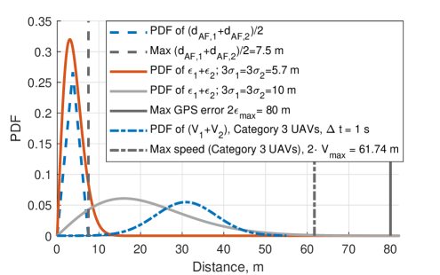
Figure 1: Caption

For demonstration purposes, as a starting point, let us assume that two UAVs broadcast their Drone IDs containing an identification number, coordinates, speed, and time stamp as specified in [Drone_ID]. Fig. 2 shows how uNMAC horizontal dimensions change while we gradually increase the amount of shared information and eliminate localization errors caused by i) absence of information about actual GNSS accuracy, ii) absence of information about movement direction, iii) GNSS and communication update rates. The minimal achievable uNMAC dimensions are defined only by the individual UAV wingspans (size). Note that i) the gradient filling indicates the uncertainty of UAV positions, ii) Fig. 2 is a simplified 2D representation, but the solution is equally valid for 3D uNMAC volume definition.

Figure 2: Different uNMAC volume definitions. Rational separation distances can be achieved by means of information exchange. Note that zero errors (indicated by green font) are not achievable in practice, but the errors can be minimized.

V Results

IEEE conference templates contain guidance text for composing and formatting conference papers. Please ensure that all template text is removed from your conference paper prior to submission to the conference. Failure to remove the template text from your paper may result in your paper not being published.