Exploring the Algorithm-Dependent Generalization of AUPRC Optimization with List Stability

Peisong Wen1,2           Qianqian Xu1          Zhiyong Yang2            
Yuan He3              Qingming Huang1,2,4,5∗
1
Key Lab of Intell. Info. Process., Inst. of Comput. Tech., CAS
2 School of Computer Science and Tech., University of Chinese Academy of Sciences 3 Alibaba Group 4 BDKM, University of Chinese Academy of Sciences 5 Peng Cheng Laboratory {wenpeisong20z,xuqianqian}@ict.ac.cn   
{yangzhiyong21,qmhuang}@ucas.ac.cn    heyuan.hy@alibaba-inc.com
Corresponding authors.
Abstract

Stochastic optimization of the Area Under the Precision-Recall Curve (AUPRC) is a crucial problem for machine learning. Although various algorithms have been extensively studied for AUPRC optimization, the generalization is only guaranteed in the multi-query case. In this work, we present the first trial in the single-query generalization of stochastic AUPRC optimization. For sharper generalization bounds, we focus on algorithm-dependent generalization. There are both algorithmic and theoretical obstacles to our destination. From an algorithmic perspective, we notice that the majority of existing stochastic estimators are biased only when the sampling strategy is biased, and is leave-one-out unstable due to the non-decomposability. To address these issues, we propose a sampling-rate-invariant unbiased stochastic estimator with superior stability. On top of this, the AUPRC optimization is formulated as a composition optimization problem, and a stochastic algorithm is proposed to solve this problem. From a theoretical perspective, standard techniques of the algorithm-dependent generalization analysis cannot be directly applied to such a listwise compositional optimization problem. To fill this gap, we extend the model stability from instancewise losses to listwise losses and bridge the corresponding generalization and stability. Additionally, we construct state transition matrices to describe the recurrence of the stability, and simplify calculations by matrix spectrum. Practically, experimental results on three image retrieval datasets on speak to the effectiveness and soundness of our framework.

1 Introduction

Area Under the Precision-Recall Curve (AUPRC) is a widely used metric in the machine learning community, especially in learning to rank, which effectively measures the trade-off between precision and recall of a ranking model. Compared with threshold-specified metrics like accuracy and recall@k, AUPRC reflects a more comprehensive performance by capturing all possible thresholds. In addition, literature has shown that AUPRC is insensitive toward data distributions [20], making it adaptable to largely skewed data. Benefiting from these appealing properties, AUPRC has become one of the standard metrics in various applications, e.g., retrieval [55, 58, 22, 41], object detection [45, 49, 15], medical diagnosis [50, 35], and recommendation systems [16, 73, 1, 64, 2].

Over the past decades, the importance of AUPRC has prompted extensive researches on direct AUPRC optimization. Early work focuses on full-batch optimization [45, 44, 26]. However, in the era of deep learning, the rapidly growing scale of models and data makes these full-batch algorithms infeasible. Therefore, in recent years, it has raised an increasing favor of the stochastic AUPRC optimization [9, 12, 31, 46]. Since AUPRC optimization is a stochastic dependent compositional optimization problem, general convergence rates are infeasible for AUPRC optimization. To fill this gap, [54, 70, 69] provide AUPRC optimization algorithms with provable convergence. See Appendix A for more on related work.

Despite the promoting performance of these methods in various scenarios, the generalization of AUPRC optimization algorithms is still an open problem. Some studies [17, 63] provide provable generalization for AUPRC optimization in information retrieval. In this scene, a dataset consists of multiple queries, where each query corresponds to a set of positive and negative samples. However, these results require sufficient queries to ensure small generalization errors, but leave the single-query case alone, i.e., whether the generalization error tends to zero with the length of a single-query increasing is still unclear. This limits the adaptation scope of these methods. To fill this gap, in this paper we aim to design a stochastic optimization framework for AUPRC with a provable algorithm-dependent generalization performance in the single-query case.

The target is challenging in three aspects: (a) Most AUPRC stochastic estimators are biased with a biased sampling rate. Moreover, due to the non-decomposability, outputs of existing algorithms might change a lot with slight changes in the training data, which is called leave-one-out unstable in this paper. Such an unstability is harmful to the generalization. (b) The standard framework to analyze the algorithm-dependent generalization requires the objective function to be expressed as a sum of instancewise terms, while AUPRC involves a listwise loss. (c) The stochastic optimization of AUPRC is a two-level compositional optimization problem, which brings more complicated proofs of the stability.

In search of a solution to (a), we propose a sampling-rate-invariant asymptotically unbiased stochastic estimator based on a reformulation of AUPRC. Notably, to ensure the stability [28, 39, 37, 38] of the estimator, the objective is formulated as a two-level compositional problem by introducing an auxiliary vector for the ranking estimation. Error analysis further supports the feasibility of our method, and inspires us to add a semi-variance regularization term. To solve this problem, we propose an algorithm with provable convergence that combines stochastic gradient descent (SGD), linear interpolation and exponential moving average.

Facing challenge (b), we extend instancewise model stability to listwise model stability, and correspondingly put forward the generalization via stability of listwise problems. On top of this, we bridge the generalization of AUPRC and the stability of the proposed optimization algorithm.

As for challenge (c), since the variables to be optimized are typically updated alternately in the compositional optimization problem, we propose state transition matrices of these variables, and simplify the calculations of the stability with matrix spectrum.

In a nutshell, the main contributions of this paper are summarized as follows:

  • Algorithmically, a stochastic learning algorithm is proposed for AUPRC optimization. The core of the proposed algorithm is a stochastic estimator which is sampling-rate-invariant asymptotically unbiased.

  • Theoretically, we present the first trial on the algorithm-dependent generalization of stochastic AUPRC optimization. To the best of our knowledge, it is also the first work to analyze the stability of stochastic compositional optimization problems.

  • Technically, we extend the concept of the stability and generalization guarantee to listwise non-convex losses. Then we simplify the stability analysis of compositional objective by matrix spectrum. These techniques might be instructive for other complicated metrics.

2 Problem Formulation

2.1 Preliminaries on AUPRC

Notations. Consider a set of N𝑁N examples 𝒮={(𝒙i,yi)}i=1N𝒮superscriptsubscriptsubscript𝒙𝑖subscript𝑦𝑖𝑖1𝑁\mathcal{S}=\{(\bm{x}_{i},y_{i})\}_{i=1}^{N} independently drawn from a sample space 𝒟=𝒳×𝒴𝒟𝒳𝒴\mathcal{D}=\mathcal{X}\times\mathcal{Y}, where 𝒳𝒳\mathcal{X} is the input space and 𝒴={1,1}𝒴11\mathcal{Y}=\{-1,1\} is the label space. For sake of the presentation, denote the set of positive examples of 𝒮𝒮\mathcal{S} as 𝒮+={𝒙i+}i=1N+superscript𝒮superscriptsubscriptsubscriptsuperscript𝒙𝑖𝑖1superscript𝑁\mathcal{S}^{+}=\{\bm{x}^{+}_{i}\}_{i=1}^{N^{+}}, and similarly the set of negative examples is denoted as 𝒮={𝒙i}i=1Nsuperscript𝒮superscriptsubscriptsubscriptsuperscript𝒙𝑖𝑖1superscript𝑁\mathcal{S}^{-}=\{\bm{x}^{-}_{i}\}_{i=1}^{N^{-}}, where N+=|𝒮+|,N=|𝒮|formulae-sequencesuperscript𝑁superscript𝒮superscript𝑁superscript𝒮N^{+}=|\mathcal{S}^{+}|,N^{-}=|\mathcal{S}^{-}|. With a slight abuse of notation, we also denote 𝒮=𝒮+𝒮𝒮superscript𝒮superscript𝒮\mathcal{S}=\mathcal{S}^{+}\cup\mathcal{S}^{-} if there is no ambiguity. Generally, we assume that the dataset is sufficiently large, such that N+/(N++N)=(y=1):=πsuperscript𝑁superscript𝑁superscript𝑁𝑦1assign𝜋N^{+}/(N^{+}+N^{-})=\mathbb{P}(y=1):=\pi. Our target is to learn a score function h𝒘:𝒳:subscript𝒘maps-to𝒳h_{\bm{w}}:\mathcal{X}\mapsto\mathbb{R} with parameters 𝒘Ωd𝒘Ωsuperscript𝑑\bm{w}\in\Omega\subseteq\mathbb{R}^{d}, such that the scores of positive examples are higher than negative examples. Furthermore, when appling the score function to a dataset 𝒮𝒳N𝒮superscript𝒳𝑁\mathcal{S}\in\mathcal{X}^{N}, we denote h𝒘:𝒳NN:subscript𝒘maps-tosuperscript𝒳𝑁superscript𝑁h_{\bm{w}}:\mathcal{X}^{N}\mapsto\mathbb{R}^{N}, where the k𝑘k-th element of h𝒘(𝒮)subscript𝒘𝒮h_{\bm{w}}(\mathcal{S}) has the top-k𝑘k values of {h𝒘(𝒙)|𝒙𝒮}conditional-setsubscript𝒘𝒙𝒙𝒮\{h_{\bm{w}}(\bm{x})|\bm{x}\in\mathcal{S}\}. Denote the asymptotic upper bound on complexity as 𝒪𝒪\mathcal{O}, and denote asymptotically equivalent as asymptotically-equals\asymp.

In this work, our main interest is to optimize a score function in the view of AUPRC:

AUPRC(𝒘;𝒟)AUPRC𝒘𝒟\displaystyle\text{AUPRC}(\bm{w};\mathcal{D}) =01(y=1|h𝒘(𝒙)c)𝑑(h𝒘(𝒙)c|y=1)absentsuperscriptsubscript01𝑦conditional1subscript𝒘𝒙𝑐differential-dsubscript𝒘𝒙conditional𝑐𝑦1\displaystyle=\int_{0}^{1}\mathbb{P}(y=1|h_{\bm{w}}(\bm{x})\geq c)~{}d~{}\mathbb{P}(h_{\bm{w}}(\bm{x})\geq c|y=1) (1)
=01πTPR(c)πTPR(c)+(1π)FPR(c)𝑑(h𝒘(𝒙)c|y=1),absentsuperscriptsubscript01𝜋𝑇𝑃𝑅𝑐𝜋𝑇𝑃𝑅𝑐1𝜋𝐹𝑃𝑅𝑐differential-dsubscript𝒘𝒙conditional𝑐𝑦1\displaystyle=\int_{0}^{1}\frac{\pi TPR(c)}{\pi TPR(c)+(1-\pi)FPR(c)}~{}d~{}\mathbb{P}(h_{\bm{w}}(\bm{x})\geq c|y=1),

where (𝒙,y)𝒟similar-to𝒙𝑦𝒟(\bm{x},y)\sim\mathcal{D}, c𝑐c refers to a threshold, and TPR(c)=(h𝒘(𝒙)c|y=1),FPR(c)=(h𝒘(𝒙)c|y=0)formulae-sequence𝑇𝑃𝑅𝑐subscript𝒘𝒙conditional𝑐𝑦1𝐹𝑃𝑅𝑐subscript𝒘𝒙conditional𝑐𝑦0TPR(c)=\mathbb{P}(h_{\bm{w}}(\bm{x})\geq c|y=1),FPR(c)=\mathbb{P}(h_{\bm{w}}(\bm{x})\geq c|y=0). For a finite set 𝒮𝒮\mathcal{S}, AUPRC is typically approximated by replacing the distribution function (h𝒘(𝒙)c|y=1)subscript𝒘𝒙conditional𝑐𝑦1\mathbb{P}(h_{\bm{w}}(\bm{x})\geq c|y=1) with its empirical cumulative distribution function [8, 19]:

AUPRC^(𝒘;𝒮)^AUPRC𝒘𝒮\displaystyle\widehat{\text{AUPRC}}(\bm{w};\mathcal{S}) =𝔼^𝒙+𝒮+[πTPR^(h𝒘(𝒙+))πTPR^(h𝒘(𝒙+))+(1π)FPR^(h𝒘(𝒙+))],absentsubscript^𝔼similar-tosuperscript𝒙superscript𝒮delimited-[]𝜋^𝑇𝑃𝑅subscript𝒘superscript𝒙𝜋^𝑇𝑃𝑅subscript𝒘superscript𝒙1𝜋^𝐹𝑃𝑅subscript𝒘superscript𝒙\displaystyle=\mathop{\hat{\mathbb{E}}}\limits_{\bm{x}^{+}\sim\mathcal{S}^{+}}\left[\frac{\pi\widehat{TPR}(h_{\bm{w}}(\bm{x}^{+}))}{\pi\widehat{TPR}(h_{\bm{w}}(\bm{x}^{+}))+(1-\pi)\widehat{FPR}(h_{\bm{w}}(\bm{x}^{+}))}\right], (2)

where TPR^(c)=𝔼^𝒙𝒮+[0,1(ch𝒘(𝒙))],FPR^(c)=𝔼^𝒙𝒮[0,1(ch𝒘(𝒙))]formulae-sequence^𝑇𝑃𝑅𝑐subscript^𝔼similar-to𝒙superscript𝒮delimited-[]subscript01𝑐subscript𝒘𝒙^𝐹𝑃𝑅𝑐subscript^𝔼similar-to𝒙superscript𝒮delimited-[]subscript01𝑐subscript𝒘𝒙\widehat{TPR}(c)=\hat{\mathbb{E}}_{\bm{x}\sim\mathcal{S}^{+}}\left[\ell_{0,1}(c-h_{\bm{w}}(\bm{x}))\right],\widehat{FPR}(c)=\hat{\mathbb{E}}_{\bm{x}\sim\mathcal{S}^{-}}\left[\ell_{0,1}(c-h_{\bm{w}}(\bm{x}))\right], 0,1(x)=1subscript01𝑥1\ell_{0,1}(x)=1 if x0𝑥0x\leq 0 or 0,1(x)=0subscript01𝑥0\ell_{0,1}(x)=0 otherwise. It has been shown that AUPRC^^AUPRC\widehat{\text{AUPRC}} is an unbiased estimator when N+/(N++N)πsuperscript𝑁superscript𝑁superscript𝑁𝜋N^{+}/(N^{+}+N^{-})\rightarrow\pi and N𝑁N\rightarrow\infty [8]. With the above estimation, we have the following optimization objective:

min𝒘AUPRC^(𝒘;𝒮)=1AUPRC^(𝒘;𝒮)=𝔼^𝒙+𝒮+[σ(1ππFPR^(hw(𝒙+))TPR^(hw(𝒙+)))],subscript𝒘superscript^AUPRC𝒘𝒮1^AUPRC𝒘𝒮subscript^𝔼similar-tosuperscript𝒙superscript𝒮delimited-[]𝜎1𝜋𝜋^𝐹𝑃𝑅subscript𝑤superscript𝒙^𝑇𝑃𝑅subscript𝑤superscript𝒙\displaystyle\min_{\bm{w}}~{}~{}~{}\widehat{\text{AUPRC}}^{\downarrow}(\bm{w};\mathcal{S})=1-\widehat{\text{AUPRC}}(\bm{w};\mathcal{S})=\mathop{\hat{\mathbb{E}}}\limits_{\bm{x}^{+}\sim\mathcal{S}^{+}}\left[\sigma\left({\color[rgb]{0,0,1}\frac{1-\pi}{\pi}}\cdot\frac{\widehat{FPR}(h_{w}(\bm{x}^{+}))}{\widehat{TPR}(h_{w}(\bm{x}^{+}))}\right)\right], (3)

where σ(x)=x/(1+x)𝜎𝑥𝑥1𝑥\sigma(x)=x/(1+x) is concave and monotonically increasing. To make it smooth, surrogate losses 1,2subscript1subscript2\ell_{1},\ell_{2} are used to replace 0,1subscript01\ell_{0,1} in FPR^^𝐹𝑃𝑅\widehat{FPR} and TPR^^𝑇𝑃𝑅\widehat{TPR} respectively, yielding the following surrogate objective:

min𝒘f(𝒘;𝒮)=𝔼^𝒙+𝒮+[σ(1ππFPR^(hw(𝒙+);1)TPR^(hw(𝒙+);2))],subscript𝒘𝑓𝒘𝒮subscript^𝔼similar-tosuperscript𝒙superscript𝒮delimited-[]𝜎1𝜋𝜋^𝐹𝑃𝑅subscript𝑤superscript𝒙subscript1^𝑇𝑃𝑅subscript𝑤superscript𝒙subscript2\displaystyle\min_{\bm{w}}~{}~{}~{}f(\bm{w};\mathcal{S})=\mathop{\hat{\mathbb{E}}}\limits_{\bm{x}^{+}\sim\mathcal{S}^{+}}\left[\sigma\left({\color[rgb]{0,0,1}\frac{1-\pi}{\pi}}\cdot\frac{\widehat{FPR}(h_{w}(\bm{x}^{+});\ell_{1})}{\widehat{TPR}(h_{w}(\bm{x}^{+});\ell_{2})}\right)\right], (4)

where TPR^(c;2)=𝔼^𝒙𝒮+[2(ch𝒘(𝒙))],FPR^(c;1)=𝔼^𝒙𝒮[1(ch𝒘(𝒙))]formulae-sequence^𝑇𝑃𝑅𝑐subscript2subscript^𝔼similar-to𝒙superscript𝒮delimited-[]subscript2𝑐subscript𝒘𝒙^𝐹𝑃𝑅𝑐subscript1subscript^𝔼similar-to𝒙superscript𝒮delimited-[]subscript1𝑐subscript𝒘𝒙\widehat{TPR}(c;\ell_{2})=\hat{\mathbb{E}}_{\bm{x}\sim\mathcal{S}^{+}}\left[\ell_{2}(c-h_{\bm{w}}(\bm{x}))\right],\widehat{FPR}(c;\ell_{1})=\hat{\mathbb{E}}_{\bm{x}\sim\mathcal{S}^{-}}\left[\ell_{1}(c-h_{\bm{w}}(\bm{x}))\right]. Specifically, when N+/(N++N)=πsuperscript𝑁superscript𝑁superscript𝑁𝜋N^{+}/(N^{+}+N^{-})=\pi, it is equivalent to another commonly used formulation Average Precision (AP) Loss:

AP^(𝒘;𝒮)=𝔼^𝒙+𝒮+[σ(𝒙𝒮[1(h𝒘(𝒙+)h𝒘(𝒙))]𝒙𝒮+[2(h𝒘(𝒙+)h𝒘(𝒙))])].superscript^AP𝒘𝒮subscript^𝔼similar-tosuperscript𝒙superscript𝒮delimited-[]𝜎subscriptsimilar-to𝒙superscript𝒮delimited-[]subscript1subscript𝒘superscript𝒙subscript𝒘𝒙subscriptsimilar-to𝒙superscript𝒮delimited-[]subscript2subscript𝒘superscript𝒙subscript𝒘𝒙\displaystyle\widehat{\text{AP}}^{\downarrow}(\bm{w};\mathcal{S})=\mathop{\hat{\mathbb{E}}}\limits_{\bm{x}^{+}\sim\mathcal{S}^{+}}\left[\sigma\left(\frac{\sum_{\bm{x}\sim\mathcal{S}^{-}}\left[\ell_{1}(h_{\bm{w}}(\bm{x}^{+})-h_{\bm{w}}(\bm{x}))\right]}{\sum_{\bm{x}\sim\mathcal{S}^{+}}\left[\ell_{2}(h_{\bm{w}}(\bm{x}^{+})-h_{\bm{w}}(\bm{x}))\right]}\right)\right]. (5)

2.2 Stochastic Learning of AUPRC

Under the stochastic learning framework for instancewise losses, the empirical risk F(𝒘;𝒮)𝐹𝒘𝒮F(\bm{w};\mathcal{S}) is expressed as a sum of instancewise losses: F(𝒘;𝒮)=1N𝒙𝒮f^(𝒘;𝒙)𝐹𝒘𝒮1𝑁subscriptsimilar-to𝒙𝒮^𝑓𝒘𝒙F(\bm{w};\mathcal{S})=\frac{1}{N}\sum_{\bm{x}\sim\mathcal{S}}\hat{f}(\bm{w};\bm{x}), where f^(𝒘;𝒙)^𝑓𝒘𝒙\hat{f}(\bm{w};\bm{x}) is the stochastic estimator of F(𝒘;𝒮)𝐹𝒘𝒮F(\bm{w};\mathcal{S}). Different from instancewise losses, listwise losses like AUPRC require a batch of samples to calculate the stochastic estimator. Specifically, at each step, a subset of 𝒮𝒮\mathcal{S}: 𝒛=𝒛+𝒛𝒛superscript𝒛superscript𝒛\bm{z}=\bm{z}^{+}\cup\bm{z}^{-} is randomly drawn, where 𝒛+superscript𝒛\bm{z}^{+} consists of n+superscript𝑛n^{+} positive examples and 𝒛superscript𝒛\bm{z}^{-} consists of nsuperscript𝑛n^{-} negative examples. Then a stochastic estimator of the loss function, denoted as f^(𝒘;𝒛)^𝑓𝒘𝒛\hat{f}(\bm{w};\bm{z}), is computed with 𝒛𝒛\bm{z}. Similar to the instancewise case, we consider a variant of the empirical/population AUPRC risks as approximations, which is a sum of stochastic losses w.r.t. all posible 𝒛𝒛\bm{z}:

F(𝒘;𝒮)=1M𝒛f^(𝒘;𝒛),F(𝒘)=𝔼𝒮𝒟[F(𝒘;𝒮)],formulae-sequence𝐹𝒘𝒮1𝑀subscript𝒛^𝑓𝒘𝒛𝐹𝒘subscript𝔼similar-to𝒮𝒟delimited-[]𝐹𝒘𝒮F(\bm{w};\mathcal{S})=\frac{1}{M}\sum_{\bm{z}}\hat{f}(\bm{w};\bm{z}),~{}~{}~{}~{}F(\bm{w})=\mathbb{E}_{\mathcal{S}\sim\mathcal{D}}[F(\bm{w};\mathcal{S})], (6)

where M𝑀M is the number of all posible 𝒛𝒛\bm{z}. Unfortunately, due to the non-decomposability of the empirical AUPRC risk f(𝒘;𝒮)𝑓𝒘𝒮f(\bm{w};\mathcal{S}), it is tackle to determine the approximation errors between F(𝒘;𝒮)𝐹𝒘𝒮F(\bm{w};\mathcal{S}) and f(𝒘;𝒮)𝑓𝒘𝒮f(\bm{w};\mathcal{S}) in general. Nonetheless, in Sec. 3.3 we argue that by selecting proper f^(𝒘;𝒛)^𝑓𝒘𝒛\hat{f}(\bm{w};\bm{z}), F(𝒘;𝒮)𝐹𝒘𝒮F(\bm{w};\mathcal{S}) can be asymptotically unbiased estimator of f(𝒘;𝒮)𝑓𝒘𝒮f(\bm{w};\mathcal{S}), which naturally makes F(𝒘)𝐹𝒘F(\bm{w}) an asymptotically unbiased estimator of 1AUPRC1AUPRC1-\text{AUPRC}. In this case, f^^𝑓\hat{f} is said to be an asymptotically unbiased stochastic estimator. Moreover, if the unbiasedness holds under biased sampling rate, it is said to be sampling-rate-invariant asymptotically unbiased.

3 Asymptotically Unbiased Stochastic AUPRC Optimization

In this section, we will present our SGD-style stochastic optimization algorithm of AUPRC. In Sec. 3.1, we propose surrogate losses to make the objective function differentiable. In Sec. 3.2, we present details of the proposed stochastic estimator and the corresponding optimization algorithm. Analyses on approximation errors are provided in Sec. 3.3.

3.1 Differentiable Surrogate Losses

Since 0,1subscript01\ell_{0,1} appears in both the numerator and denominator of Eq. (4), simply implementing 1,2subscript1subscript2\ell_{1},\ell_{2} with a single function [56, 9, 54] will bring difficulty to analyze the relationship between AUPRC^(𝒘;𝒮)superscript^AUPRC𝒘𝒮\widehat{\text{AUPRC}}^{\downarrow}(\bm{w};\mathcal{S}) and f(𝒘;𝒮)𝑓𝒘𝒮f(\bm{w};\mathcal{S}). This motivates us to choose 10,1,20,1formulae-sequencesubscript1subscript01subscript2subscript01\ell_{1}\geq\ell_{0,1},\ell_{2}\leq\ell_{0,1}, such that AUPRC^(𝒘;𝒮)f(𝒘;𝒮)superscript^AUPRC𝒘𝒮𝑓𝒘𝒮\widehat{\text{AUPRC}}^{\downarrow}(\bm{w};\mathcal{S})\leq f(\bm{w};\mathcal{S}), thus the original empirical risk could be optimized by minimizing its upper bound f(𝒘;𝒮)𝑓𝒘𝒮f(\bm{w};\mathcal{S}). Concretely, 1subscript1\ell_{1} and 2subscript2\ell_{2} are defined as the one-side Huber loss and the one-side sigmoid loss:

1(x)={2x/τ1,x<0,(1x/τ1)2,0x<τ1,0,xτ1.2(x)={exp(x/τ2)1exp(x/τ2)+1,x<0,0,x0.formulae-sequencesubscript1𝑥casesmissing-subexpression2𝑥subscript𝜏1𝑥0missing-subexpressionsuperscript1𝑥subscript𝜏120𝑥subscript𝜏1missing-subexpression0𝑥subscript𝜏1missing-subexpressionsubscript2𝑥casesmissing-subexpression𝑥subscript𝜏21𝑥subscript𝜏21𝑥0missing-subexpression0𝑥0missing-subexpression\ell_{1}(x)=\left\{\begin{array}[]{cc}\begin{aligned} &-2x/\tau_{1},&x<0,\\ &(1-x/\tau_{1})^{2},&0\leq x<\tau_{1},\\ &0,&x\geq\tau_{1}.\end{aligned}\end{array}\right.~{}~{}~{}~{}~{}~{}~{}~{}~{}\ell_{2}(x)=\left\{\begin{array}[]{cc}\begin{aligned} &\frac{\exp(-x/\tau_{2})-1}{\exp(-x/\tau_{2})+1},&x<0,\\ &0,&x\geq 0.\end{aligned}\end{array}\right. (7)

Here τ1,τ2>0subscript𝜏1subscript𝜏20\tau_{1},\tau_{2}>0 are hyperparameters. 1subscript1\ell_{1} is convex and decreasing, which ensures the gap between positive-negative pairs is effectively optimized. Additionally, compared with the square loss and the exponential loss, 1subscript1\ell_{1} is more robust to noises. 2subscript2\ell_{2} is Lipschitz continuous, and 20,1subscript2subscript01\ell_{2}\rightarrow\ell_{0,1} with τ20subscript𝜏20\tau_{2}\rightarrow 0.

3.2 Stochastic Estimator of AUPRC

The key to a stochastic learning framework is the design of the stochastic estimator (or the corresponding gradients), i.e., f^(𝒘;𝒛)^𝑓𝒘𝒛\hat{f}(\bm{w};\bm{z}). Existing methods [9, 74, 12] implement it with AP^(𝒘;𝒛)superscript^AP𝒘𝒛\widehat{\text{AP}}^{\downarrow}(\bm{w};\bm{z}) (Eq. (5)), which might suffer from two problems:

  • (P1)

    Comparing Eq. (4) and Eq. (5), it can be seen that only when n+/(n++n)πsuperscript𝑛superscript𝑛superscript𝑛𝜋n^{+}/(n^{+}+n^{-})\rightarrow\pi, AP^superscript^AP\widehat{\text{AP}}^{\downarrow} is an asymptotically unbiased estimator. However, it is hardly satisfied since the sampling strategy is usually biased in practice.

  • (P2)

    Each term in the summation of AP^superscript^AP\widehat{\text{AP}}^{\downarrow} is related to all instances of a batch, leading to weak leave-one-out stability, i.e., changing one instance might result in a relatively large fluctuation in the stochastic gradient, especially when changing a positive example.

To tackle the above problems, we first substitute FPR^(hw(𝒙+);1)^𝐹𝑃𝑅subscript𝑤superscript𝒙subscript1\widehat{FPR}(h_{w}(\bm{x}^{+});\ell_{1}) with 𝔼^𝒙𝒛[1(h𝒘(𝒙+)h𝒘(𝒙))]subscript^𝔼similar-to𝒙superscript𝒛delimited-[]subscript1subscript𝒘superscript𝒙subscript𝒘𝒙\mathop{\hat{\mathbb{E}}}_{\bm{x}\sim\bm{z}^{-}}[\ell_{1}(h_{\bm{w}}(\bm{x}^{+})-h_{\bm{w}}(\bm{x}))], and then introduce an auxiliary vector 𝒗N+𝒗superscriptsuperscript𝑁\bm{v}\in\mathbb{R}^{N^{+}} to estimate TPR^^𝑇𝑃𝑅\widehat{TPR}. Formally, we propose the following batch-based estimator:

f^(𝒘;𝒛)=f^(𝒘;𝒛,𝒗)=𝔼^𝒙+𝒛+[σ(1ππ𝔼^𝒙𝒛[1(h𝒘(𝒙+)h𝒘(𝒙))]𝔼^v𝒗[2(h𝒘(𝒙+)v)])].^𝑓𝒘𝒛^𝑓𝒘𝒛𝒗subscript^𝔼similar-tosuperscript𝒙superscript𝒛delimited-[]𝜎1𝜋𝜋subscript^𝔼similar-to𝒙superscript𝒛delimited-[]subscript1subscript𝒘superscript𝒙subscript𝒘𝒙subscript^𝔼similar-to𝑣𝒗delimited-[]subscript2subscript𝒘superscript𝒙𝑣\hat{f}(\bm{w};\bm{z})=\hat{f}(\bm{w};\bm{z},\bm{v})=\mathop{\hat{\mathbb{E}}}\limits_{\bm{x}^{+}\sim\bm{z}^{+}}\left[\sigma\left({\color[rgb]{0,0,1}\frac{1-\pi}{\pi}}\cdot\frac{\mathop{\hat{\mathbb{E}}}_{\bm{x}\sim\bm{z}^{-}}[\ell_{1}(h_{\bm{w}}(\bm{x}^{+})-h_{\bm{w}}(\bm{x}))]}{\mathop{\hat{\mathbb{E}}}_{v\sim\bm{v}}[\ell_{2}(h_{\bm{w}}(\bm{x}^{+})-v)]}\right)\right]. (8)

Such an estimator enjoys two advantages: in terms of P1, it is asymptotically unbiased regardless of the sampling rate (see Sec. 3.3 for detailed discussions); as for P2, we use 𝒗𝒗\bm{v} to substitute h𝒘(𝒮+)subscript𝒘superscript𝒮h_{\bm{w}}(\mathcal{S}^{+}), such that each positive example in a mini-batch only appears in one term. Ideally, it can be considered as using all positive examples in the dataset to estimate TPR^^𝑇𝑃𝑅\widehat{TPR} instead of that from a mini-batch. With the fact that nn+much-greater-thansuperscript𝑛superscript𝑛n^{-}\gg n^{+}, this makes the corresponding algorithm more stable. Moreover, based on the model stability, generalization bounds are available (see Sec. 4).

3.3 Analyses on Approximation Errors

In this subsection, we analyze errors from two approximations in the above algorithm: 1) the gap between F(𝒘;𝒮)𝐹𝒘𝒮F(\bm{w};\mathcal{S}) and the true AUPRC loss; 2) the gap between the interpolated scores ϕ(h𝒘(𝒛+))italic-ϕsubscript𝒘superscript𝒛\phi(h_{\bm{w}}(\bm{z}^{+})) and the true scores h𝒘(𝒮+)subscript𝒘superscript𝒮h_{\bm{w}}(\mathcal{S}^{+}). Proofs are provided in Appendix B.1.

Denote π=N+/(N++N)𝜋superscript𝑁superscript𝑁superscript𝑁\pi=N^{+}/(N^{+}+N^{-}) and π0=n+/(n++n)subscript𝜋0superscript𝑛superscript𝑛superscript𝑛\pi_{0}=n^{+}/(n^{+}+n^{-}). We would like to show that for all 𝒘Ω𝒘Ω\bm{w}\in\Omega, 𝔼𝒛[f^(𝒘;𝒛)]subscript𝔼𝒛delimited-[]^𝑓𝒘𝒛\mathbb{E}_{\bm{z}}[\hat{f}(\bm{w};\bm{z})] is an unbiased estimator when n𝑛n\rightarrow\infty, no matter how π0subscript𝜋0\pi_{0} is chosen, while for 𝔼𝒛[AP^(𝒘;𝒛)]subscript𝔼𝒛delimited-[]superscript^AP𝒘𝒛\mathbb{E}_{\bm{z}}[\widehat{\text{AP}}^{\downarrow}(\bm{w};\bm{z})], it holds only when π0=πsubscript𝜋0𝜋\pi_{0}=\pi. Since only one model 𝒘𝒘\bm{w} is considered, we let 𝒘t=𝒘subscript𝒘𝑡𝒘\bm{w}_{t}=\bm{w} in the update rule of 𝒗𝒗\bm{v} (Eq. (10)), and we have the following proposition:

Proposition 1.

Consider updating 𝐯𝐯\bm{v} with Eq. (10) for T𝑇T steps, then we have

𝔼[𝒗]=𝔼[ϕ(h𝒘(𝒛+))]+(1β)T(𝒗1𝔼[ϕ(h𝒘(𝒛+))]),Var[𝒗]Var[ϕ(h𝒘(𝒛+))]β2β.formulae-sequence𝔼delimited-[]𝒗𝔼delimited-[]italic-ϕsubscript𝒘superscript𝒛superscript1𝛽𝑇subscript𝒗1𝔼delimited-[]italic-ϕsubscript𝒘superscript𝒛𝑉𝑎𝑟delimited-[]𝒗𝑉𝑎𝑟delimited-[]italic-ϕsubscript𝒘superscript𝒛𝛽2𝛽\mathbb{E}[\bm{v}]=\mathbb{E}[\phi(h_{\bm{w}}(\bm{z}^{+}))]+(1-\beta)^{T}\left(\bm{v}_{1}-\mathbb{E}[\phi\left(h_{\bm{w}}(\bm{z}^{+})\right)]\right),~{}~{}Var[\bm{v}]\leq Var[\phi(h_{\bm{w}}(\bm{z}^{+}))]\cdot\frac{\beta}{2-\beta}.
Remark 1.

Two conclusions could be drawn from the above proposition: first, if the linear interpolation is asymptotically unbiased (see next subsection), by choosing a large T𝑇T or setting 𝐯1=𝔼[ϕ(h𝐰(𝐳+))]subscript𝐯1𝔼delimited-[]italic-ϕsubscript𝐰superscript𝐳\bm{v}_{1}=\mathbb{E}[\phi(h_{\bm{w}}(\bm{z}^{+}))], we have 𝔼[𝐯]h𝐰(𝒮+)𝔼delimited-[]𝐯subscript𝐰superscript𝒮\mathbb{E}[\bm{v}]\approx h_{\bm{w}}(\mathcal{S}^{+}); second, by choosing a smaller ββ\beta, 𝐯𝐯\bm{v} is more likely to concentrate on h𝐰(𝒮+)subscripth𝐰superscript𝒮h_{\bm{w}}(\mathcal{S}^{+}).

Proposition 2.

Assume the linear interpolation is asymptotically unbiased. Let κ12=𝔼^ch𝐰(𝐳+)[Var𝐱𝒮[1(ch𝐰(𝐱))]]subscriptsuperscript𝜅21subscript^𝔼similar-to𝑐subscript𝐰superscript𝐳delimited-[]𝑉𝑎subscript𝑟similar-to𝐱superscript𝒮delimited-[]subscript1𝑐subscript𝐰𝐱\kappa^{2}_{1}=\mathop{\hat{\mathbb{E}}}_{c\sim h_{\bm{w}}(\bm{z}^{+})}[Var_{\bm{x}\sim\mathcal{S}^{-}}[\ell_{1}\left(c-h_{\bm{w}}(\bm{x})\right)]], κ22=𝔼^ch𝐰(𝐳+)[Varv𝐯[2(cv))]]\kappa^{2}_{2}=\mathop{\hat{\mathbb{E}}}_{c\sim h_{\bm{w}}(\bm{z}^{+})}[Var_{v\sim\bm{v}}[\ell_{2}\left(c-v)\right)]]. When κ12/n0subscriptsuperscript𝜅21superscript𝑛0\kappa^{2}_{1}/n^{-}\rightarrow 0, κ22/n+0subscriptsuperscript𝜅22superscript𝑛0\kappa^{2}_{2}/n^{+}\rightarrow 0, then there exists a positive scale H𝐻H, such that

𝔼^𝒛𝒮[f^(𝒘;𝒛)]𝑃AUPRC^(𝒘;𝒮),𝔼^𝒛𝒮[AP^(𝒘;𝒛)]𝑃(1+(π0π)H)AUPRC^(𝒘;𝒮),subscript^𝔼𝒛𝒮delimited-[]^𝑓𝒘𝒛𝑃superscript^AUPRC𝒘𝒮subscript^𝔼𝒛𝒮delimited-[]superscript^AP𝒘𝒛𝑃1subscript𝜋0𝜋𝐻superscript^AUPRC𝒘𝒮\displaystyle\hat{\mathbb{E}}_{\bm{z}\subseteq\mathcal{S}}[\hat{f}(\bm{w};\bm{z})]\overset{P}{\rightarrow}\widehat{\text{AUPRC}}^{\downarrow}(\bm{w};\mathcal{S}),~{}~{}\hat{\mathbb{E}}_{\bm{z}\subseteq\mathcal{S}}\left[\widehat{\text{AP}}^{\downarrow}(\bm{w};\bm{z})\right]\overset{P}{\rightarrow}\left(1+(\pi_{0}-\pi)H\right)\cdot\widehat{\text{AUPRC}}^{\downarrow}(\bm{w};\mathcal{S}),

where 𝑃𝑃\overset{P}{\rightarrow} refers to convergence in probability, and 𝐳𝒮𝐳𝒮\bm{z}\subseteq\mathcal{S} refers to subsets described in Sec. 2.2.

Remark 2.

The above proposition suggests that the proposed batch-based estimator is sampling-rate-invariant asymptotically unbiased, while AP^superscript^AP\widehat{\text{AP}}^{\downarrow} tends to be larger when the sampling rate of the positive class is greater than the prior, and vice versa. We also provide a non-asymptotic result in Appendix B.2.

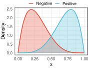
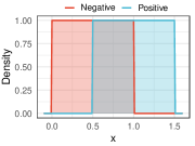
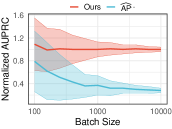
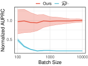
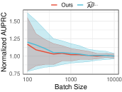
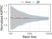
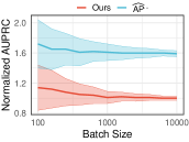
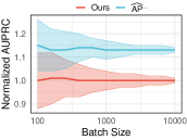
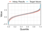
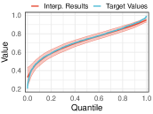
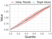
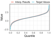
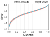
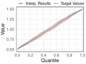
Simulation experiments are conducted as complementary to the theory. Following previous work [8], the scores are drawn from three types of distributions, including binormal, bibeta and offset uniform. The results of binormal distribution are visualized in Fig. 1, and detailed descriptions and more results are available in Appendix B.2. These results are consistent with the above remark.

Next we further study the interpolation error. For the sake of presentation, denote p:[0,1]:𝑝maps-to01p:[0,1]\mapsto\mathbb{R} to be an increasing score function describing h𝒘(𝒮+)subscript𝒘superscript𝒮h_{\bm{w}}(\mathcal{S}^{+}), where p(x)𝑝𝑥p(x) is the score in the bottom x𝑥x-quantile of h𝒘(𝒮+)subscript𝒘superscript𝒮h_{\bm{w}}(\mathcal{S}^{+}). Similarly, let p^^𝑝\hat{p} to be the interpolation results of 𝔼A[h𝒘(𝒛+)]subscript𝔼𝐴delimited-[]subscript𝒘superscript𝒛\mathbb{E}_{A}[h_{\bm{w}}(\bm{z}^{+})]. Assume that 𝔼A[h𝒘(𝒛+)]subscript𝔼𝐴delimited-[]subscript𝒘superscript𝒛\mathbb{E}_{A}[h_{\bm{w}}(\bm{z}^{+})] are located in the (i/n+)𝑖superscript𝑛(i/n^{+})-quantiles of p𝑝p, where i[n+]𝑖delimited-[]superscript𝑛i\in[n^{+}], such that p(i/n+)=p^(i/n+)𝑝𝑖superscript𝑛^𝑝𝑖superscript𝑛p(i/n^{+})=\hat{p}(i/n^{+}) and all interpolation intervals are with length 1/n+1superscript𝑛1/n^{+}. The following proposition provides an upper bound of the approximation error (see [61] for proof):

Proposition 3 (Linear Interpolation Error).

Let p,p^𝑝^𝑝p,\hat{p} be defined as above. Then we have

pp^p′′/(8(n+)2).subscriptnorm𝑝^𝑝subscriptnormsuperscript𝑝′′8superscriptsuperscript𝑛2\|p-\hat{p}\|_{\infty}\leq\|p^{\prime\prime}\|_{\infty}/\left(8(n^{+})^{2}\right).

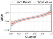
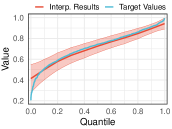
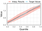
Similar to the last subsection, simulation results are shown in Fig. 1(c), which shows the expected errors of linear interpolation are ignorable.

Refer to caption
(a) Density functions of scores.
Refer to captionRefer to caption
(b) Stochastic Estimation Errors with π0=0.02subscript𝜋00.02\pi_{0}=0.02 (left) and π0=0.2subscript𝜋00.2\pi_{0}=0.2 (right).
Refer to caption
(c) Interpolation Errors with π0=0.03subscript𝜋00.03\pi_{0}=0.03.
Figure 1: Empirical analysis of estimation errors on simulation data.

3.4 Optimization Algorithm

In the rest of this section, we focus on how to optimize F(𝒘;𝒮)𝐹𝒘𝒮F(\bm{w};\mathcal{S}). The main challenge is to design update rules for 𝒗𝒗\bm{v}, such that it could efficiently and effectively approximate h𝒘(𝒮+)subscript𝒘superscript𝒮h_{\bm{w}}(\mathcal{S}^{+}) without full-batch scanning. To overcome the challenge, we propose an algorithm called Stochastic Optimization of AUPRC (SOPRC), which jointly updates model parameters 𝒘𝒘\bm{w} and the auxiliary vector 𝒗𝒗\bm{v}. A summary of the detailed process is shown as Alg. 1. At step t𝑡t, a batch of data is sampled from the training set, and then compute the corresponding scores. Afterward, scores of positive examples are mapped into a N+superscript𝑁N^{+}-dimension vector with linear interpolation ϕitalic-ϕ\phi as shown in Alg. 2. 𝒗t+1subscript𝒗𝑡1\bm{v}_{t+1} are updated with the interpolated scores in a moving average manner.

Practically, n+,nsuperscript𝑛superscript𝑛n^{+},n^{-} are finite, causing inevitable estimation errors in f(𝒘;𝒛it,𝒗t+1)𝑓𝒘subscript𝒛subscript𝑖𝑡subscript𝒗𝑡1f(\bm{w};\bm{z}_{i_{t}},\bm{v}_{t+1}). Notice that another factor influencing the stochastic estimation errors, i.e., κ12subscriptsuperscript𝜅21\kappa^{2}_{1} and κ22subscriptsuperscript𝜅22\kappa^{2}_{2}. To reduce them, it is expected that the variance of positive (negative) scores are small, which motivates us to add a variance regularization term. However, it might force to reduce positive scores that higher than the mean value, which is contrary to our target. Therefore, we propose a semi-variance regularization term [4]:

var=λ1n+𝒙𝒛+h𝒘(𝒙)<μ+(h𝒘(𝒙)μ+)2+λ2n𝒙𝒛h𝒘(𝒙)>μ(h𝒘(𝒙)μ)2,subscript𝑣𝑎𝑟subscript𝜆1superscript𝑛subscriptFRACOPsimilar-to𝒙superscript𝒛subscript𝒘𝒙superscript𝜇superscriptsubscript𝒘𝒙superscript𝜇2subscript𝜆2superscript𝑛subscriptFRACOPsimilar-to𝒙superscript𝒛subscript𝒘𝒙superscript𝜇superscriptsubscript𝒘𝒙superscript𝜇2\mathcal{L}_{var}=\frac{\lambda_{1}}{n^{+}}\sum_{\bm{x}\sim\bm{z}^{+}\atop h_{\bm{w}}(\bm{x})<\mu^{+}}(h_{\bm{w}}(\bm{x})-\mu^{+})^{2}+\frac{\lambda_{2}}{n^{-}}\sum_{\bm{x}\sim\bm{z}^{-}\atop h_{\bm{w}}(\bm{x})>\mu^{-}}(h_{\bm{w}}(\bm{x})-\mu^{-})^{2}, (9)

where μ+=1n+𝒙𝒛+h𝒘(𝒙)superscript𝜇1superscript𝑛subscriptsimilar-to𝒙superscript𝒛subscript𝒘𝒙\mu^{+}=\frac{1}{n^{+}}\sum_{\bm{x}\sim\bm{z}^{+}}h_{\bm{w}}(\bm{x}), μ=1n𝒙𝒛h𝒘(𝒙)superscript𝜇1superscript𝑛subscriptsimilar-to𝒙superscript𝒛subscript𝒘𝒙\mu^{-}=\frac{1}{n^{-}}\sum_{\bm{x}\sim\bm{z}^{-}}h_{\bm{w}}(\bm{x}), λ1,λ2subscript𝜆1subscript𝜆2\lambda_{1},\lambda_{2} are hyperparameters. Finally, we compute the gradients of f(𝒘;𝒛it,𝒗t+1)+var𝑓𝒘subscript𝒛subscript𝑖𝑡subscript𝒗𝑡1subscript𝑣𝑎𝑟f(\bm{w};\bm{z}_{i_{t}},\bm{v}_{t+1})+\mathcal{L}_{var}, and update parameters 𝒘𝒘\bm{w} with gradient descent.

Algorithm 1 SOPRC
0:  Training dataset 𝒮𝒮\mathcal{S}, maximum iterations T𝑇T, learning rate {ηt}t=1Tsuperscriptsubscriptsubscript𝜂𝑡𝑡1𝑇\{\eta_{t}\}_{t=1}^{T} and {βt}t=1Tsuperscriptsubscriptsubscript𝛽𝑡𝑡1𝑇\{\beta_{t}\}_{t=1}^{T}.
0:  model parameters 𝒘T+1subscript𝒘𝑇1\bm{w}_{T+1}.
1:  Initialize model parameters 𝒘1subscript𝒘1\bm{w}_{1} and 𝒗1subscript𝒗1\bm{v}_{1}.
2:  for t=1𝑡1t=1 to T𝑇T do
3:     Sample a subset 𝒛itsubscript𝒛subscript𝑖𝑡\bm{z}_{i_{t}} from 𝒮𝒮\mathcal{S}.
4:     Compute h𝒘t(𝒛it+)subscriptsubscript𝒘𝑡subscriptsuperscript𝒛subscript𝑖𝑡h_{\bm{w}_{t}}(\bm{z}^{+}_{i_{t}}) and map the results into ϕ(h𝒘t(𝒛it+))italic-ϕsubscriptsubscript𝒘𝑡subscriptsuperscript𝒛subscript𝑖𝑡\phi(h_{\bm{w}_{t}}(\bm{z}^{+}_{i_{t}})) with Alg. 2.
5:     Update 𝒗𝒗\bm{v} with
𝒗t+1=subscript𝒗𝑡1absent\displaystyle\bm{v}_{t+1}= (1βt)𝒗t1subscript𝛽𝑡subscript𝒗𝑡\displaystyle(1-\beta_{t})\bm{v}_{t} (10)
+βtϕ(h𝒘t(𝒛it+)).subscript𝛽𝑡italic-ϕsubscriptsubscript𝒘𝑡subscriptsuperscript𝒛subscript𝑖𝑡\displaystyle~{}~{}+\beta_{t}\phi(h_{\bm{w}_{t}}(\bm{z}^{+}_{i_{t}})).
6:     Compute varsubscript𝑣𝑎𝑟\mathcal{L}_{var} with Eq. (9).
7:     Update the model parameter:
𝒘t+1=subscript𝒘𝑡1absent\displaystyle\bm{w}_{t+1}= 𝒘tηtvarsubscript𝒘𝑡subscript𝜂𝑡subscript𝑣𝑎𝑟\displaystyle\bm{w}_{t}-\eta_{t}\cdot\nabla\mathcal{L}_{var} (11)
ηtf(𝒘t;𝒛it,𝒗t+1).subscript𝜂𝑡𝑓subscript𝒘𝑡subscript𝒛subscript𝑖𝑡subscript𝒗𝑡1\displaystyle-\eta_{t}\cdot\nabla f(\bm{w}_{t};\bm{z}_{i_{t}},\bm{v}_{t+1}).
8:  end for
Algorithm 2 Score Interpolation ϕ()italic-ϕ\phi(\cdot)
0:  A real value vector 𝒖n𝒖superscript𝑛\bm{u}\in\mathbb{R}^{n} where n<N+𝑛superscript𝑁n<N^{+}, range of target values [b,B]𝑏𝐵[b,B].
0:  Interpolated vector 𝒎=ϕ(𝒖)𝒎italic-ϕ𝒖\bm{m}=\phi(\bm{u}).
1:  Sort 𝒖𝒖\bm{u} in descending order.
2:  Initialize 𝒎𝒎\bm{m} as 𝟎N+subscript0superscript𝑁\bm{0}_{N^{+}}, let u0=max(2u1u2,b),un+1=min(2un2un1,B)formulae-sequencesubscript𝑢0𝑚𝑎𝑥2subscript𝑢1subscript𝑢2𝑏subscript𝑢𝑛1𝑚𝑖𝑛2subscript𝑢𝑛2subscript𝑢𝑛1𝐵u_{0}=max(2u_{1}-u_{2},b),u_{n+1}=min(2u_{n}-2u_{n-1},B).
3:  for i=1𝑖1i=1 to n𝑛n do
4:     for j=N+(i1)n𝑗superscript𝑁𝑖1𝑛j=\lceil\frac{N^{+}(i-1)}{n}\rceil to [N+in]delimited-[]superscript𝑁𝑖𝑛\left[\frac{N^{+}\cdot i}{n}\right] do
5:          
mj+=limit-fromsubscript𝑚𝑗absent\displaystyle m_{j}+= [(ijn/N+)ui1\displaystyle\left[(i-jn/N^{+})u_{i-1}\right.
+(1+jn/N+i)ui]/2\displaystyle\left.+(1+jn/N^{+}-i)u_{i}\right]/2
6:     end for
7:     for j=[N+in]𝑗delimited-[]superscript𝑁𝑖𝑛j=\left[\frac{N^{+}\cdot i}{n}\right] to N+(i+1)nsuperscript𝑁𝑖1𝑛\lfloor\frac{N^{+}\cdot(i+1)}{n}\rfloor do
8:         
mj+=limit-fromsubscript𝑚𝑗absent\displaystyle m_{j}+= [(i+1jn/N+)ui1\displaystyle\left[(i+1-jn/N^{+})u_{i-1}\right.
+(jn/N+i)ui]/2\displaystyle\left.+(jn/N^{+}-i)u_{i}\right]/2
9:     end for
10:  end for

4 Generalization of SOPRC via Stability

In this section, we turn to study the excess generalization error of the proposed algorithm. Formally, following standard settings [5], we consider the test error of the model A(𝒮)𝐴𝒮A(\mathcal{S}) trained on the training set 𝒮𝒮\mathcal{S}. Our target is to seek an upper bound of the excess error 𝔼A,𝒮[F(A(𝒮))F(𝒘)]subscript𝔼𝐴𝒮delimited-[]𝐹𝐴𝒮𝐹superscript𝒘\mathbb{E}_{A,\mathcal{S}}[F(A(\mathcal{S}))-F(\bm{w}^{*})], where 𝒘argmin𝒘Ω𝔼A,𝒮[F(𝒘)]superscript𝒘subscript𝒘Ωsubscript𝔼𝐴𝒮delimited-[]𝐹superscript𝒘\bm{w}^{*}\in\arg\min_{\bm{w}\in\Omega}\mathbb{E}_{A,\mathcal{S}}[F(\bm{w}^{*})]. It can be decomposed as:

𝔼𝒮,A[F(A(𝒮))F(𝒘)]=𝔼𝒮,A[F(A(𝒮))F(A(𝒮);𝒮)]Estimation Error+𝔼𝒮,A[F(A(𝒮);𝒮)F(𝒘)]Optimization Error.subscript𝔼𝒮𝐴delimited-[]𝐹𝐴𝒮𝐹superscript𝒘subscriptsubscript𝔼𝒮𝐴delimited-[]𝐹𝐴𝒮𝐹𝐴𝒮𝒮Estimation Errorsubscriptsubscript𝔼𝒮𝐴delimited-[]𝐹𝐴𝒮𝒮𝐹superscript𝒘Optimization Error\mathbb{E}_{\mathcal{S},A}[F(A(\mathcal{S}))-F(\bm{w}^{*})]=\underbrace{\mathbb{E}_{\mathcal{S},A}[F(A(\mathcal{S}))-F(A(\mathcal{S});\mathcal{S})]}_{\textit{Estimation Error}}+\underbrace{\mathbb{E}_{\mathcal{S},A}[F(A(\mathcal{S});\mathcal{S})-F(\bm{w}^{*})]}_{\textit{Optimization Error}}.

The estimation error sources from the gap of minimizing the empirical risk instead of the expected risk. In Sec. 4.1, we provide detailed discussion on the estimation error. The optimization error measures the gap between the minimum empirical risk and the results obtained by the optimization algorithm, which will be studied in Sec. 4.2. Detailed proofs of this section are available in Appendix C. Before the formal presentation, we show the main assumptions:

Assumption 1 (Bounded Scores & Gradient).

|f^(𝒘;)|B,f^(𝒘;)2Gformulae-sequence^𝑓𝒘𝐵subscriptnorm^𝑓𝒘2𝐺|\hat{f}(\bm{w};\cdot)|\leq B,\|\nabla\hat{f}(\bm{w};\cdot)\|_{2}\leq G for all 𝐰Ω𝐰Ω\bm{w}\in\Omega.

Assumption 2 (L-Smooth Loss).

f^(𝒘;)f^(𝒘~;)2L𝒘𝒘~2subscriptnorm^𝑓𝒘^𝑓~𝒘2𝐿subscriptnorm𝒘~𝒘2\|\nabla\hat{f}(\bm{w};\cdot)-\nabla\hat{f}(\tilde{\bm{w}};\cdot)\|_{2}\leq L\|\bm{w}-\tilde{\bm{w}}\|_{2} for all 𝐰,𝐰~Ω𝐰~𝐰Ω\bm{w},\tilde{\bm{w}}\in\Omega.

Assumption 3 (Lipschitz Continuous Functions).

|1(x)1(x~)|L1|xx~|subscript1𝑥subscript1~𝑥subscript𝐿1𝑥~𝑥|\ell_{1}(x)-\ell_{1}(\tilde{x})|\leq L_{1}|x-\tilde{x}|, |2(x)2(x~)|L2|xx~|subscript2𝑥subscript2~𝑥subscript𝐿2𝑥~𝑥|\ell_{2}(x)-\ell_{2}(\tilde{x})|\leq L_{2}|x-\tilde{x}| for all x,x~[2B,2B]𝑥~𝑥2𝐵2𝐵x,\tilde{x}\in[-2B,2B]. ϕ(𝐱)ϕ(𝐱~)2Cϕ𝐱𝐱~2subscriptnormitalic-ϕ𝐱italic-ϕ~𝐱2subscript𝐶italic-ϕsubscriptnorm𝐱~𝐱2\|\phi(\bm{x})-\phi(\tilde{\bm{x}})\|_{2}\leq C_{\phi}\|\bm{x}-\tilde{\bm{x}}\|_{2} for all 𝐱,𝐱~N+𝐱~𝐱superscriptsuperscript𝑁\bm{x},\tilde{\bm{x}}\in\mathbb{R}^{N^{+}}.

4.1 Generalization of AUPRC via Model Stability

The generalization of SGD-style algorithms for instancewise loss has been widely studied with stability measure [39, 21, 28]. However, these results could not be directly applied to listwise losses like AUPRC. The main reason is that the estimation of each stochastic gradient requires a list of examples, and the estimation is usually biased. Nonetheless, to bridge the optimization algorithm and the generalization of AUPRC, we propose a listwise variant of on-average model stability [39] as follows:

Definition 1 (Listwise On-average Model Stability).

Let 𝒮={(𝐱i,yi)}i=1N𝒮superscriptsubscriptsubscript𝐱𝑖subscript𝑦𝑖𝑖1𝑁\mathcal{S}=\{(\bm{x}_{i},y_{i})\}_{i=1}^{N} and 𝒮~={(𝐱~i,yi)}i=1N~𝒮superscriptsubscriptsubscript~𝐱𝑖subscript𝑦𝑖𝑖1𝑁\widetilde{\mathcal{S}}=\{(\widetilde{\bm{x}}_{i},y_{i})\}_{i=1}^{N} be two sets of examples whose features are drawn independently from 𝒳𝒳\mathcal{X}. For any i=1,,N𝑖1𝑁i=1,\cdots,N, denote 𝒮(i)={(𝐱1,y1),,(𝐱i1,yi1),(𝐱~i,yi),(𝐱i+1,yi+1),,(𝐱n,yn)}superscript𝒮𝑖subscript𝐱1subscript𝑦1subscript𝐱𝑖1subscript𝑦𝑖1subscript~𝐱𝑖subscript𝑦𝑖subscript𝐱𝑖1subscript𝑦𝑖1subscript𝐱𝑛subscript𝑦𝑛\mathcal{S}^{(i)}=\{(\bm{x}_{1},y_{1}),\cdots,(\bm{x}_{i-1},y_{i-1}),(\widetilde{\bm{x}}_{i},y_{i}),(\bm{x}_{i+1},y_{i+1}),\cdots,(\bm{x}_{n},y_{n})\}. A stochastic algorithm A𝐴A is listwise on-average model (ϵ+,ϵ)superscriptitalic-ϵsuperscriptitalic-ϵ(\epsilon^{+},\epsilon^{-})-stable if the following condition holds:

𝔼𝒮,𝒮~,A[1N+yi=1A(𝒮)A(𝒮(i))2]ϵ+,𝔼𝒮,𝒮~,A[1Nyi=1A(𝒮)A(𝒮(i))2]ϵ.formulae-sequencesubscript𝔼𝒮~𝒮𝐴delimited-[]1superscript𝑁subscriptsubscript𝑦𝑖1subscriptnorm𝐴𝒮𝐴superscript𝒮𝑖2superscriptitalic-ϵsubscript𝔼𝒮~𝒮𝐴delimited-[]1superscript𝑁subscriptsubscript𝑦𝑖1subscriptnorm𝐴𝒮𝐴superscript𝒮𝑖2superscriptitalic-ϵ\displaystyle\mathbb{E}_{\mathcal{S},\widetilde{\mathcal{S}},A}\left[\frac{1}{N^{+}}\sum_{y_{i}=1}\left\|\ A(\mathcal{S})-A(\mathcal{S}^{(i)})\right\|_{2}\right]\leq\epsilon^{+},\mathbb{E}_{\mathcal{S},\widetilde{\mathcal{S}},A}\left[\frac{1}{N^{-}}\sum_{y_{i}=-1}\left\|\ A(\mathcal{S})-A(\mathcal{S}^{(i)})\right\|_{2}\right]\leq\epsilon^{-}.

The following theorem shows that the estimation error is bounded by the above-defined stability:

Theorem 1 (Generalization via Model Stability).

Let a stochastic algorithm A𝐴A be listwise on-average model (ϵ+,ϵ)superscriptitalic-ϵsuperscriptitalic-ϵ(\epsilon^{+},\epsilon^{-})-stable and Asmp. 1 holds. Then we have

𝔼𝒮,A[F(A(𝒮))F(A(𝒮);𝒮)]G(n+ϵ++nϵ).subscript𝔼𝒮𝐴delimited-[]𝐹𝐴𝒮𝐹𝐴𝒮𝒮𝐺superscript𝑛superscriptitalic-ϵsuperscript𝑛superscriptitalic-ϵ\mathbb{E}_{\mathcal{S},A}\left[F(A(\mathcal{S}))-F(A(\mathcal{S});\mathcal{S})\right]\leq G(n^{+}\epsilon^{+}+n^{-}\epsilon^{-}). (12)

With the above theorem, now we only need to focus on the model stability of the proposed algorithm. Notice that in Alg. 1, both 𝒘tsubscript𝒘𝑡\bm{w}_{t} and 𝒗tsubscript𝒗𝑡\bm{v}_{t} are updated at each step, thus we have to consider the stability of both simultaneously. The following lemma provides a recurrence for the stability 𝒘tsubscript𝒘𝑡\bm{w}_{t} and 𝒗tsubscript𝒗𝑡\bm{v}_{t}.

Lemma 1.

Let 𝒮,𝒮~,𝒮(i)𝒮~𝒮superscript𝒮𝑖\mathcal{S},\widetilde{\mathcal{S}},\mathcal{S}^{(i)} be constructed as Def. 1 and Asmp. 1, 2, 3 hold. Let {𝐰t}tsubscriptsubscript𝐰𝑡𝑡\{\bm{w}_{t}\}_{t} and {𝐰t(i)}tsubscriptsuperscriptsubscript𝐰𝑡𝑖𝑡\{\bm{w}_{t}^{(i)}\}_{t} be produced by Alg. 1 with 𝒮𝒮\mathcal{S} and 𝒮(i)superscript𝒮𝑖\mathcal{S}^{(i)}, respectively. Denote L=max{Lw,Lv/n+,CϕB,G/2,B}𝐿subscript𝐿𝑤subscript𝐿𝑣superscript𝑛subscript𝐶italic-ϕ𝐵𝐺2subscriptsuperscript𝐵L=\max\{L_{w},L_{v}/n^{+},C_{\phi}B,G/2,B^{\prime}_{\ell}\}, 𝐦t(i)=[𝐰t𝐰t(i)2𝐯t𝐯t(i)21]superscriptsubscript𝐦𝑡𝑖superscriptdelimited-[]subscriptnormsubscript𝐰𝑡superscriptsubscript𝐰𝑡𝑖2subscriptnormsubscript𝐯𝑡superscriptsubscript𝐯𝑡𝑖21top\bm{m}_{t}^{(i)}=\left[\begin{array}[]{ccc}\|\bm{w}_{t}-\bm{w}_{t}^{(i)}\|_{2}&\|\bm{v}_{t}-\bm{v}_{t}^{(i)}\|_{2}&1\end{array}\right]^{\top}, 𝐦t+=1N+yi=1𝔼𝒮,A[𝐦t(i)]superscriptsubscript𝐦𝑡1superscript𝑁subscriptsubscript𝑦𝑖1subscript𝔼𝒮𝐴delimited-[]superscriptsubscript𝐦𝑡𝑖\bm{m}_{t}^{+}=\frac{1}{N^{+}}\sum_{y_{i}=1}\mathbb{E}_{\mathcal{S},A}\left[\bm{m}_{t}^{(i)}\right], 𝐦t=1N+yi=1𝔼𝒮,A[𝐦t(i)]superscriptsubscript𝐦𝑡1superscript𝑁subscriptsubscript𝑦𝑖1subscript𝔼𝒮𝐴delimited-[]superscriptsubscript𝐦𝑡𝑖\bm{m}_{t}^{-}=\frac{1}{N^{+}}\sum_{y_{i}=-1}\mathbb{E}_{\mathcal{S},A}\left[\bm{m}_{t}^{(i)}\right]. Then for all t[T]𝑡delimited-[]𝑇t\in[T], by setting βt2CϕB/n+subscript𝛽𝑡2subscript𝐶italic-ϕ𝐵superscript𝑛\beta_{t}\leq 2C_{\phi}B/n^{+}, we have

𝒎t+1+(𝑰3+𝑹t+)𝒎t+,𝒎t+1(𝑰3+𝑹t)𝒎t,formulae-sequencesuperscriptsubscript𝒎𝑡1subscript𝑰3subscriptsuperscript𝑹𝑡superscriptsubscript𝒎𝑡superscriptsubscript𝒎𝑡1subscript𝑰3subscriptsuperscript𝑹𝑡superscriptsubscript𝒎𝑡\bm{m}_{t+1}^{+}\leq\left(\bm{I}_{3}+\bm{R}^{+}_{t}\right)\cdot\bm{m}_{t}^{+},~{}~{}~{}~{}~{}~{}\bm{m}_{t+1}^{-}\leq\left(\bm{I}_{3}+\bm{R}^{-}_{t}\right)\cdot\bm{m}_{t}^{-}, (13)

where 𝐈3subscript𝐈3\bm{I}_{3} is the 3×3333\times 3 identity matrix and

Rt+subscriptsuperscript𝑅𝑡\displaystyle R^{+}_{t} =[2LηtL(1βt)ηtN+LηtN+Lβt01N+000],Rtabsentdelimited-[]2𝐿subscript𝜂𝑡𝐿1subscript𝛽𝑡subscript𝜂𝑡superscript𝑁𝐿subscript𝜂𝑡superscript𝑁𝐿subscript𝛽𝑡01superscript𝑁000subscriptsuperscript𝑅𝑡\displaystyle=\left[\begin{array}[]{ccc}2L\eta_{t}&\frac{L(1-\beta_{t})\eta_{t}}{N^{+}}&\frac{L\eta_{t}}{N^{+}}\\ L\beta_{t}&0&\frac{1}{N^{+}}\\ 0&0&0\end{array}\right],R^{-}_{t} =[2LηtLv(1βt)ηtN+Lηtn+NLβt00000].absentdelimited-[]2𝐿subscript𝜂𝑡subscript𝐿𝑣1subscript𝛽𝑡subscript𝜂𝑡superscript𝑁𝐿subscript𝜂𝑡superscript𝑛superscript𝑁𝐿subscript𝛽𝑡00000\displaystyle=\left[\begin{array}[]{ccc}2L\eta_{t}&\frac{L_{v}(1-\beta_{t})\eta_{t}}{N^{+}}&\frac{L\eta_{t}\cdot n^{+}}{N^{-}}\\ L\beta_{t}&0&0\\ 0&0&0\end{array}\right]. (14)

Finally, we utilize the matrix spectrum of Rt+subscriptsuperscript𝑅𝑡R^{+}_{t} and Rtsubscriptsuperscript𝑅𝑡R^{-}_{t} to show that the model stability w.r.t. Alg. 1 decreases as the number of training examples increases (see Appendix C.2 for details):

Theorem 2.

Let λ=LCη(1+1β2+β)𝜆𝐿subscript𝐶𝜂11superscript𝛽2𝛽\lambda=LC_{\eta}(1+\sqrt{1-\beta^{2}+\beta}), and assumptions in Lem. 1 hold. By setting ηtCηtsubscript𝜂𝑡subscript𝐶𝜂𝑡\eta_{t}\leq\frac{C_{\eta}}{t}, βt=β1/n+subscript𝛽𝑡𝛽asymptotically-equals1superscript𝑛\beta_{t}=\beta\asymp 1/n^{+} and TN+𝑇superscript𝑁T\leq N^{+}, Alg. 1 is list on-average model stable with

ϵ+=𝒪((Tn+)λλ+1N+),ϵ=𝒪((Tn)λλ+1N).formulae-sequencesuperscriptitalic-ϵ𝒪superscript𝑇superscript𝑛𝜆𝜆1superscript𝑁superscriptitalic-ϵ𝒪superscript𝑇superscript𝑛𝜆𝜆1superscript𝑁\displaystyle\epsilon^{+}=\mathcal{O}\left(\frac{\left(Tn^{+}\right)^{\frac{\lambda}{\lambda+1}}}{N^{+}}\right),\epsilon^{-}=\mathcal{O}\left(\frac{\left(Tn^{-}\right)^{\frac{\lambda}{\lambda+1}}}{N^{-}}\right). (15)

4.2 Convergence of AUPRC Stochastic Optimization

Following previous work [24, 34], we study the optimization error of the proposed algorithm under the Polyak-Łojasiewicz (PL) condition. It has been shown that the PL condition holds for several widely used models including some classes of neural networks [13, 42].

Assumption 4 (Polyak-Łojasiewicz Condition [34, 37]).

Denote 𝐰=argmin𝐰ΩF(𝐰)superscript𝐰subscript𝐰Ω𝐹𝐰\bm{w}^{*}=\arg\min_{\bm{w}\in\Omega}F(\bm{w}). Assume F𝐹F satisfy the expectation version of PL condition with parameter μ>0𝜇0\mu>0, i.e.,

𝔼𝒮[F(𝒘;𝒮)F(𝒘)]1μ𝔼𝒮[F(𝒘;𝒮)22].subscript𝔼𝒮delimited-[]𝐹𝒘𝒮𝐹superscript𝒘1𝜇subscript𝔼𝒮delimited-[]superscriptsubscriptnorm𝐹𝒘𝒮22\mathbb{E}_{\mathcal{S}}[F(\bm{w};\mathcal{S})-F(\bm{w}^{*})]\leq\frac{1}{\mu}\mathbb{E}_{\mathcal{S}}[\|\nabla F(\bm{w};\mathcal{S})\|_{2}^{2}]. (16)

The main difference to the existing convergence analysis on non-convex optimization is that the gradient estimation is biased. Nonetheless, we show that the bias terms from Alg. 1 tend to 00 with sufficient training data and training time (see Appendix C.3), leading to the following convergence:

Theorem 3.

Let Asmp. 1, 3, 4 hold. By setting ηt=2t+1μ(t+1)2subscript𝜂𝑡2𝑡1𝜇superscript𝑡12\eta_{t}=\frac{2t+1}{\mu(t+1)^{2}} and βt=β1/n+subscript𝛽𝑡𝛽asymptotically-equals1superscript𝑛\beta_{t}=\beta\asymp 1/n^{+}, we have

𝔼A[F(𝒘T+1)F(𝒘)]=𝒪(n+/T+1/N+).subscript𝔼𝐴delimited-[]𝐹subscript𝒘𝑇1𝐹superscript𝒘𝒪superscript𝑛𝑇1superscript𝑁\displaystyle\mathbb{E}_{A}[F(\bm{w}_{T+1})-F(\bm{w}^{*})]=\mathcal{O}\left(n^{+}/T+1/N^{+}\right). (17)
Theorem 4.

Let assumptions in Thm. 2 and 3 hold. By setting T(N+)λ+12λ+1(n+)12λ+1asymptotically-equals𝑇superscriptsuperscript𝑁𝜆12𝜆1superscriptsuperscript𝑛12𝜆1T\asymp(N^{+})^{\frac{\lambda+1}{2\lambda+1}}(n^{+})^{-\frac{1}{2\lambda+1}}, we have

𝔼𝒮,A[F(A(𝒮))F(𝒘)]=𝒪((N+)λ+12λ+1(n+)3λ+12λ+1)+𝒪((N)λ+12λ+1(n)3λ+12λ+1).subscript𝔼𝒮𝐴delimited-[]𝐹𝐴𝒮𝐹superscript𝒘𝒪superscriptsuperscript𝑁𝜆12𝜆1superscriptsuperscript𝑛3𝜆12𝜆1𝒪superscriptsuperscript𝑁𝜆12𝜆1superscriptsuperscript𝑛3𝜆12𝜆1\mathbb{E}_{\mathcal{S},A}[F(A(\mathcal{S}))-F(\bm{w}^{*})]=\mathcal{O}\left((N^{+})^{-\frac{\lambda+1}{2\lambda+1}}\cdot(n^{+})^{\frac{3\lambda+1}{2\lambda+1}}\right)+\mathcal{O}\left((N^{-})^{-\frac{\lambda+1}{2\lambda+1}}\cdot(n^{-})^{\frac{3\lambda+1}{2\lambda+1}}\right). (18)
Remark 3.

Recall that λ=LCη(1+1β2+β)𝜆𝐿subscript𝐶𝜂11superscript𝛽2𝛽\lambda=LC_{\eta}(1+\sqrt{1-\beta^{2}+\beta}) and Cη=4/μsubscript𝐶𝜂4𝜇C_{\eta}=4/\mu, when β𝛽\beta is small, we have λ4L/μ𝜆4𝐿𝜇\lambda\approx 4L/\mu. Here L/μ𝐿𝜇L/\mu is a condition number determined by the model and surrogate losses. Notice that n+N+,nNformulae-sequencemuch-less-thansuperscript𝑛superscript𝑁much-less-thansuperscript𝑛superscript𝑁n^{+}\ll N^{+},n^{-}\ll N^{-}, if λ=1𝜆1\lambda=1, the generalization bound is 𝒪((N+)2/3(n+)4/3+(N)2/3(n)4/3)𝒪superscriptsuperscript𝑁23superscriptsuperscript𝑛43superscriptsuperscript𝑁23superscriptsuperscript𝑛43\mathcal{O}\left((N^{+})^{-2/3}\cdot(n^{+})^{4/3}+(N^{-})^{-2/3}\cdot(n^{-})^{4/3}\right). As λ𝜆\lambda increases, it increases to 𝒪((N+)1/2(n+)3/2+(N)1/2(n)3/2)𝒪superscriptsuperscript𝑁12superscriptsuperscript𝑛32superscriptsuperscript𝑁12superscriptsuperscript𝑛32\mathcal{O}\left((N^{+})^{-1/2}\cdot(n^{+})^{3/2}+(N^{-})^{-1/2}\cdot(n^{-})^{3/2}\right).

Table 1: Quantitative results on SOP, iNaturalist, and VehicleID. All methods are trained with training sets. The best and the second best results are highlighted in soft red and soft blue, respectively.
Methods Stanford Online Products iNaturalist PKU VehicleID
mAUPRC R@1 R@10 mAUPRC R@1 R@4 mAUPRC R@1 R@5
Contrastive loss [27] 57.73 77.60 89.31 27.99 54.19 71.12 67.26 87.46 94.60
Triplet loss [32] 58.07 78.34 90.50 30.59 60.53 77.62 70.99 90.09 95.54
MS loss [71] 60.10 79.64 90.38 30.28 63.39 78.50 69.15 88.82 95.06
XBM [72] 61.29 80.66 91.08 27.46 59.12 75.18 71.24 92.78 95.83
SmoothAP [9] 61.65 81.13 92.02 33.92 66.13 80.93 72.28 91.31 96.05
DIR [58] 60.74 80.52 91.35 33.51 64.86 79.79 72.72 91.38 96.10
FastAP [12] 57.10 77.30 89.61 31.02 56.64 73.57 70.82 89.42 95.38
AUROC [25] 55.80 77.32 89.64 27.24 60.88 77.76 58.12 81.73 91.92
BlackBox [52] 59.74 79.48 90.74 29.28 56.88 74.10 70.92 90.14 95.52
Ours 62.75 81.91 92.50 36.16 68.22 82.86 74.92 92.56 96.43

5 Experiments

To validate the effectiveness of the proposed method, we conduct empirical studies on the image retrieval task, in which data distributions are largely skewed and AUPRC is commonly used as an evaluation metric. More detailed experimental settings are provided in Appendix D.1. The source code is available in https://github.com/KID-7391/SOPRC.git.

5.1 Implementation Details

Datasets. We evaluate the proposed method on three image retrieval benchmarks with various domains and scales, including Stanford Online Products (SOP)111https://github.com/rksltnl/Deep-Metric-Learning-CVPR16. Licensed MIT. [48], PKU VehicleID222https://www.pkuml.org/resources/pku-vehicleid.html. Data files ©  Original Authors. [43] and iNaturalist333https://github.com/visipedia/inatcomp/tree/master/2018. Licensed MIT. [68]. We follow the official setting to split a test set from each dataset, and then further split the rest into a training set and a validation set by a ratio of 9:1:919:1.

Network Architecture. The feature extractor is implemented with ResNet-50 [29] pretrained on ImageNet [60]. Following previous work [12, 9], the batch normalization layers are fixed during training, and the output embeddings are mapped to 512-d with a linear projection. Given L2subscript𝐿2L_{2} normalized embeddings of a query image 𝒆qsubscript𝒆𝑞\bm{e}_{q} and a gallery list {𝒆i}isubscriptsubscript𝒆𝑖𝑖\{\bm{e}_{i}\}_{i}, the scores are represented by the cosine similarity 𝒆q𝒆isuperscriptsubscript𝒆𝑞topsubscript𝒆𝑖\bm{e}_{q}^{\top}\bm{e}_{i} for all i𝑖i.

Optimization Strategy. In the training phase, the input images are resized such that the sizes of the shorter sides are 256. Afterward, we applied standard data augmentations including random cropping (224×224224224224\times 224) and random flipping (50%percent5050\%). The model parameters are optimized in an end-to-end manner as shown in Alg. 1, where β=0.001𝛽0.001\beta=0.001 and the weight decay is set to 4×1044superscript1044\times 10^{-4}. The default batch size is set to 224, where each mini-batch is randomly sampled such that there are exactly 4 positive examples per category. The learning rates are tuned according to performance on validation sets: for SOP, the learning rate are initialized as 0.010.010.01 and decays by 0.10.10.1 at the 15k15𝑘15k and 30k30𝑘30k iterations, T=50k𝑇50𝑘T=50k; for VehicleID, the learning rate are initialized as 0.0010.0010.001 and decays by 0.10.10.1 at the 40k40𝑘40k and 80k80𝑘80k iterations, T=100k𝑇100𝑘T=100k; for iNaturalist, the learning rate are initialized as 0.0010.0010.001 and decays by 0.10.10.1 at the 80k80𝑘80k and 110k110𝑘110k iterations, T=130k𝑇130𝑘T=130k.

Competitors. We compare two types of competitors: 1) Pairwise Losses, including Contrastive Loss [27], Triplet Loss [32], Multi-Similarity (MS) Loss [71], Cross-Batch Memory (XBM) [72]. These methods construct loss functions with image pairs or triplets. 2) Ranking-Based Losses, including SmoothAP [9], FastAP [12], DIR [58], BlackBox [33], and Area Under the ROC Curve Loss (AUROC) [76]. These methods directly optimize the ranking-based metrics.

Evaluation Metrics. In all experiments, we adopt evaluation metrics: mean AUPRC (mAUPRC) and Recall@k. mAUPRC is also called mean average precision (mAP) in literature, which takes the mean value over the AUPRC of all queries. Recall@k measures the probability that at least one positive example is ranked in the top-k list.

5.2 Main Results

We evaluate all methods with mean AUPRC (mAUPRC) and Recall@k. mAUPRC measures the mean value of the AUPRC over all queries, a.k.a. mean average precision (mAP). The performance comparisons on test sets are shown in Tab. 1. Consequently, we have the following observations: 1) In all datasets, the proposed method surpasses all competitors in the view of mAUPRC, especially in the large-scale long-tailed dataset iNaturalist. This validates the advantages of our method in boosting the AUPRC of models. 2) Compared to pairwise losses, the AUPRC/AP optimization methods enjoy better performance generally. The main reason is that pairwise losses could only optimize models indirectly by constraining relative scores between positive and negative example pairs, while ignoring the overall ranking. 3) Although some pairwise methods like XBM have a satisfying performance on Recall@1, their mAUPRC is relatively low. It is caused by the limitation of Recall@1, i.e., it focuses on the top-1 score while ignoring the ranking of other examples. What’s more, this phenomenon shows the inconsistency of Recall@k and AUPRC, revealing the necessity of studying AUPRC optimization. More results are available in Appendix D.2.

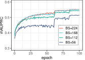
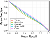
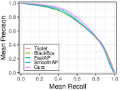
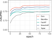
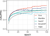
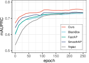
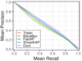
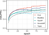
To qualitatively demonstrate the effect of the proposed method, we also show the mean PR curves and convergence curves in Fig. 2. The left two subfigures demonstrate that the proposed method achieves can effectively improve AUPRC. The right subfigure shows the affect of batch size, from which can be seen that a large batch size leads to better performance. One of the reasons is that a small batch size will amplify the AUPRC stochastic estimation error. Such a problem have been addressed by maintaining inner gradient estimations in a moving average manner [54, 70, 75]. Unfortunately, when applied to image retrieval problems, it needs to maintain intermediate variables for each sample pair, which will bring high complexity in time and space, thus we leave this problem as further work.
Refer to caption
Refer to caption
Refer to caption
Figure 2: Qualitative results on iNaturalist. Left most: mean PR curves of different methods. Right two: convergence of different methods and batch sizes in terms of mAUPRC in the validation set.

5.3 Ablation Studies

Table 2: Ablation study over different components of our method on iNaturalist.
No. Unb. Est. with 𝒗tsubscript𝒗𝑡\bm{v}_{t} with varsubscript𝑣𝑎𝑟\mathcal{L}_{var} Opt. mAUPRC R@1 R@4 R@16 R@32
1 SGD 34.58 66.35 81.04 89.80 92.72
2 SGD 35.84 67.08 81.68 90.17 92.98
3 SGD 35.99 67.50 82.03 90.44 93.26
4 SGD 36.16 68.22 82.86 91.02 93.71
5 Adam 36.20 68.48 82.70 90.96 93.63

We further investigate the effect of different components of the proposed method. Results are shown in Tab. 2, and more detailed statements and analyses are as follows.
Effect of Unbiased Estimator. To show the performance drop caused by the biased estimator, we replace the prior π𝜋\pi in Eq. (8) with n+/(n++n)superscript𝑛superscript𝑛superscript𝑛n^{+}/(n^{+}+n^{-}). Comparing line 1 and line 2, using the unbiased estimator increases the mAUPRC by 1.3%, which is consistent with our theoretical results in Sec. 3.3. Notably, the unbiased estimator is the main source of improvements in terms of mAUPRC.
Effect of vtsubscript𝑣𝑡\bm{v}_{t}. To show the effect of introducing 𝒗tsubscript𝒗𝑡\bm{v}_{t} to estimate ϕ(𝒮+)italic-ϕsuperscript𝒮\phi(\mathcal{S}^{+}), we directly use ϕ(𝒛+)italic-ϕsuperscript𝒛\phi(\bm{z}^{+}) instead in the first two lines. Comparing line 2 and line 3, using 𝒗tsubscript𝒗𝑡\bm{v}_{t} could bring consistent improvements due to the better generalization ability.
Effect of varsubscript𝑣𝑎𝑟\mathcal{L}_{var}. We show that shrinking variances could reduce the batch-based estimation errors. Comparing line 3 and line 4, it can be seen that varsubscript𝑣𝑎𝑟\mathcal{L}_{var} further boosts the proposed method.
Effect of Optimizer. Comparing line 4 and line 5, it can be seen that the choice of optimizer only has a slight influence.

6 Conclusion & Future Work

In this paper, we present a stochastic learning framework for AUPRC optimization. To begin with, we propose a stochastic AUPRC optimization algorithm based on an asymptotically unbiased stochastic estimator. By introducing an auxiliary vector to approximate the scores of positive examples, the proposed algorithm is more stable. On top of this, we study algorithm-dependent generalization. First, we propose list model stability to handle listwise losses like AUPRC, and bridge the generalization and the stability. Afterward, we show that the proposed algorithm is stable, leading to an upper bound of the generalization error. Experiments on three benchmarks validate the advantages of the proposed framework. One limitation is the convergence rate is controlled by the scale of the dataset. In the further, we will consider techniques like variance reduction to improve the convergence rate, and jointly consider the corresponding algorithm-dependent generalization.

Acknowledgments

This work was supported in part by the National Key R&D Program of China under Grant 2018AAA0102000, in part by National Natural Science Foundation of China: U21B2038, 61931008, 6212200758 and 61976202, in part by the Fundamental Research Funds for the Central Universities, in part by Youth Innovation Promotion Association CAS, in part by the Strategic Priority Research Program of Chinese Academy of Sciences, Grant No. XDB28000000, in part by the China National Postdoctoral Program for Innovative Talents under Grant BX2021298, and in part by China Postdoctoral Science Foundation under Grant 2022M713101.

References

  • [1] Shilong Bao, Qianqian Xu, Ke Ma, Zhiyong Yang, Xiaochun Cao, and Qingming Huang. Collaborative preference embedding against sparse labels. In ACM International Conference on Multimedia, pages 2079–2087, 2019.
  • [2] Shilong Bao, Qianqian Xu, Zhiyong Yang, Xiaochun Cao, and Qingming Huang. Rethinking collaborative metric learning: Toward an efficient alternative without negative sampling. IEEE Transactions on Pattern Analysis and Machine Intelligence, 2022.
  • [3] Peter L Bartlett and Shahar Mendelson. Rademacher and gaussian complexities: Risk bounds and structural results. Journal of Machine Learning Research, 3(Nov):463–482, 2002.
  • [4] Shaun A Bond and Stephen E Satchell. Statistical properties of the sample semi-variance. Applied Mathematical Finance, 9(4):219–239, 2002.
  • [5] Léon Bottou and Olivier Bousquet. The tradeoffs of large scale learning. Advances in Neural Information Processing Systems, 20, 2007.
  • [6] Stéphane Boucheron, Gábor Lugosi, and Pascal Massart. Concentration inequalities: A nonasymptotic theory of independence. Oxford university press, 2013.
  • [7] Olivier Bousquet and André Elisseeff. Stability and generalization. Journal of Machine Learning Research, 2:499–526, 2002.
  • [8] Kendrick Boyd, Kevin H Eng, and C David Page. Area under the precision-recall curve: point estimates and confidence intervals. In ECML PKDD, pages 451–466. Springer, 2013.
  • [9] Andrew Brown, Weidi Xie, Vicky Kalogeiton, and Andrew Zisserman. Smooth-ap: Smoothing the path towards large-scale image retrieval. In European Conference on Computer Vision, pages 677–694. Springer, 2020.
  • [10] Christopher Burges, Robert Ragno, and Quoc Le. Learning to rank with nonsmooth cost functions. Advances in Neural Information Processing Systems, 19:193–200, 2006.
  • [11] Christopher JC Burges. From ranknet to lambdarank to lambdamart: An overview. Learning, 11(23-581):81, 2010.
  • [12] Fatih Cakir, Kun He, Xide Xia, Brian Kulis, and Stan Sclaroff. Deep metric learning to rank. In IEEE/CVF Conference on Computer Vision and Pattern Recognition, pages 1861–1870, 2019.
  • [13] Zachary Charles and Dimitris Papailiopoulos. Stability and generalization of learning algorithms that converge to global optima. In International Conference on Machine Learning, pages 745–754. PMLR, 2018.
  • [14] Kean Chen, Jianguo Li, Weiyao Lin, John See, Ji Wang, Lingyu Duan, Zhibo Chen, Changwei He, and Junni Zou. Towards accurate one-stage object detection with ap-loss. In IEEE/CVF Conference on Computer Vision and Pattern Recognition, pages 5119–5127, 2019.
  • [15] Kean Chen, Weiyao Lin, John See, Ji Wang, Junni Zou, et al. Ap-loss for accurate one-stage object detection. IEEE Transactions on Pattern Analysis and Machine Intelligence, 2020.
  • [16] Ting Chen, Yizhou Sun, Yue Shi, and Liangjie Hong. On sampling strategies for neural network-based collaborative filtering. In ACM SIGKDD International Conference on Knowledge Discovery and Data Mining, pages 767–776, 2017.
  • [17] Wei Chen, Tie-Yan Liu, Yanyan Lan, Zhi-Ming Ma, and Hang Li. Ranking measures and loss functions in learning to rank. Advances in Neural Information Processing Systems, 22:315–323, 2009.
  • [18] Yuansi Chen, Chi Jin, and Bin Yu. Stability and convergence trade-off of iterative optimization algorithms. arXiv preprint arXiv:1804.01619, 2018.
  • [19] Stéphan Clémençon and Nicolas Vayatis. Nonparametric estimation of the precision-recall curve. In International Conference on Machine Learning, pages 185–192, 2009.
  • [20] Jesse Davis and Mark Goadrich. The relationship between precision-recall and roc curves. In International Conference on Machine Learning, pages 233–240, 2006.
  • [21] Andre Elisseeff, Theodoros Evgeniou, Massimiliano Pontil, and Leslie Pack Kaelbing. Stability of randomized learning algorithms. Journal of Machine Learning Research, 6(1), 2005.
  • [22] Martin Engilberge, Louis Chevallier, Patrick Pérez, and Matthieu Cord. Sodeep: a sorting deep net to learn ranking loss surrogates. In IEEE/CVF Conference on Computer Vision and Pattern Recognition, pages 10792–10801, 2019.
  • [23] Dylan J Foster, Spencer Greenberg, Satyen Kale, Haipeng Luo, Mehryar Mohri, and Karthik Sridharan. Hypothesis set stability and generalization. Advances in Neural Information Processing Systems, 32, 2019.
  • [24] Dylan J Foster, Ayush Sekhari, and Karthik Sridharan. Uniform convergence of gradients for non-convex learning and optimization. Advances in Neural Information Processing Systems, 31, 2018.
  • [25] Wei Gao and Zhi-Hua Zhou. On the consistency of auc pairwise optimization. In International Conference on Machine Learning, 2015.
  • [26] Mark Goadrich, Louis Oliphant, and Jude Shavlik. Gleaner: Creating ensembles of first-order clauses to improve recall-precision curves. Machine Learning, 64(1-3):231–261, 2006.
  • [27] Raia Hadsell, Sumit Chopra, and Yann LeCun. Dimensionality reduction by learning an invariant mapping. In IEEE/CVF Conference on Computer Vision and Pattern Recognition, volume 2, pages 1735–1742. IEEE, 2006.
  • [28] Moritz Hardt, Ben Recht, and Yoram Singer. Train faster, generalize better: Stability of stochastic gradient descent. In International Conference on Machine Learning, pages 1225–1234, 2016.
  • [29] Kaiming He, Xiangyu Zhang, Shaoqing Ren, and Jian Sun. Deep residual learning for image recognition. In IEEE/CVF Conference on Computer Vision and Pattern Recognition, pages 770–778, 2016.
  • [30] Kun He, Fatih Cakir, Sarah Adel Bargal, and Stan Sclaroff. Hashing as tie-aware learning to rank. In IEEE/CVF Conference on Computer Vision and Pattern Recognition, pages 4023–4032, 2018.
  • [31] Paul Henderson and Vittorio Ferrari. End-to-end training of object class detectors for mean average precision. In Asian Conference on Computer Vision, pages 198–213. Springer, 2016.
  • [32] Elad Hoffer and Nir Ailon. Deep metric learning using triplet network. In International workshop on similarity-based pattern recognition, pages 84–92. Springer, 2015.
  • [33] Qijia Jiang, Olaoluwa Adigun, Harikrishna Narasimhan, Mahdi Milani Fard, and Maya Gupta. Optimizing black-box metrics with adaptive surrogates. In International Conference on Machine Learning, pages 4784–4793. PMLR, 2020.
  • [34] Hamed Karimi, Julie Nutini, and Mark Schmidt. Linear convergence of gradient and proximal-gradient methods under the polyak-łojasiewicz condition. In Joint European Conference on Machine Learning and Knowledge Discovery in Databases, pages 795–811. Springer, 2016.
  • [35] Joon-myoung Kwon, Youngnam Lee, Yeha Lee, Seungwoo Lee, and Jinsik Park. An algorithm based on deep learning for predicting in-hospital cardiac arrest. Journal of the American Heart Association, 7(13):e008678, 2018.
  • [36] Yunwen Lei, Antoine Ledent, and Marius Kloft. Sharper generalization bounds for pairwise learning. Advances in Neural Information Processing Systems, 33:21236–21246, 2020.
  • [37] Yunwen Lei, Mingrui Liu, and Yiming Ying. Generalization guarantee of sgd for pairwise learning. Advances in Neural Information Processing Systems, 34, 2021.
  • [38] Yunwen Lei, Zhenhuan Yang, Tianbao Yang, and Yiming Ying. Stability and generalization of stochastic gradient methods for minimax problems. In International Conference on Machine Learning, pages 6175–6186. PMLR, 2021.
  • [39] Yunwen Lei and Yiming Ying. Fine-grained analysis of stability and generalization for stochastic gradient descent. In International Conference on Machine Learning, pages 5809–5819, 2020.
  • [40] Jian Li, Xuanyuan Luo, and Mingda Qiao. On generalization error bounds of noisy gradient methods for non-convex learning. In International Conference on Learning Representations, 2019.
  • [41] Zhuo Li, Weiqing Min, Jiajun Song, Yaohui Zhu, Liping Kang, Xiaoming Wei, Xiaolin Wei, and Shuqiang Jiang. Rethinking the optimization of average precision: Only penalizing negative instances before positive ones is enough. arXiv preprint arXiv:2102.04640, 2021.
  • [42] Chaoyue Liu, Libin Zhu, and Mikhail Belkin. Loss landscapes and optimization in over-parameterized non-linear systems and neural networks. Applied and Computational Harmonic Analysis, 2022.
  • [43] Hongye Liu, Yonghong Tian, Yaowei Wang, Lu Pang, and Tiejun Huang. Deep relative distance learning: Tell the difference between similar vehicles. In IEEE/CVF Conference on Computer Vision and Pattern Recognition, pages 2167–2175, 2016.
  • [44] Donald Metzler and W Bruce Croft. A markov random field model for term dependencies. In International ACM SIGIR Conference on Research and Development in Information Retrieval, pages 472–479, 2005.
  • [45] Pritish Mohapatra, CV Jawahar, and M Pawan Kumar. Efficient optimization for average precision svm. Advances in Neural Information Processing Systems, 27:2312–2320, 2014.
  • [46] Pritish Mohapatra, Michal Rolinek, CV Jawahar, Vladimir Kolmogorov, and M Pawan Kumar. Efficient optimization for rank-based loss functions. In IEEE/CVF Conference on Computer Vision and Pattern Recognition, pages 3693–3701, 2018.
  • [47] Wenlong Mou, Liwei Wang, Xiyu Zhai, and Kai Zheng. Generalization bounds of sgld for non-convex learning: Two theoretical viewpoints. In Conference on Learning Theory, pages 605–638. PMLR, 2018.
  • [48] Hyun Oh Song, Yu Xiang, Stefanie Jegelka, and Silvio Savarese. Deep metric learning via lifted structured feature embedding. In IEEE/CVF Conference on Computer Vision and Pattern Recognition, pages 4004–4012, 2016.
  • [49] Kemal Oksuz, Baris Can Cam, Emre Akbas, and Sinan Kalkan. A ranking-based, balanced loss function unifying classification and localisation in object detection. In Advances in Neural Information Processing Systems, 2020.
  • [50] Brice Ozenne, Fabien Subtil, and Delphine Maucort-Boulch. The precision–recall curve overcame the optimism of the receiver operating characteristic curve in rare diseases. Journal of clinical epidemiology, 68(8):855–859, 2015.
  • [51] Adam Paszke, Sam Gross, Francisco Massa, Adam Lerer, James Bradbury, Gregory Chanan, Trevor Killeen, Zeming Lin, Natalia Gimelshein, Luca Antiga, et al. Pytorch: An imperative style, high-performance deep learning library. Advances in Neural Information Processing Systems, 32:8026–8037, 2019.
  • [52] Marin Vlastelica Pogančić, Anselm Paulus, Vit Musil, Georg Martius, and Michal Rolinek. Differentiation of blackbox combinatorial solvers. In International Conference on Learning Representations, 2019.
  • [53] Tomaso Poggio and Christian R Shelton. On the mathematical foundations of learning. American Mathematical Society, 39(1):1–49, 2002.
  • [54] Qi Qi, Youzhi Luo, Zhao Xu, Shuiwang Ji, and Tianbao Yang. Stochastic optimization of areas under precision-recall curves with provable convergence. Advances in Neural Information Processing Systems, 34, 2021.
  • [55] Tao Qin, Tie-Yan Liu, and Hang Li. A general approximation framework for direct optimization of information retrieval measures. Information Retrieval, 13(4):375–397, 2010.
  • [56] Tao Qin, Xu-Dong Zhang, Ming-Feng Tsai, De-Sheng Wang, Tie-Yan Liu, and Hang Li. Query-level loss functions for information retrieval. Information Processing & Management, 44(2):838–855, 2008.
  • [57] Vijay Raghavan, Peter Bollmann, and Gwang S Jung. A critical investigation of recall and precision as measures of retrieval system performance. ACM Transactions on Information Systems, 7(3):205–229, 1989.
  • [58] Jerome Revaud, Jon Almazán, Rafael S Rezende, and Cesar Roberto de Souza. Learning with average precision: Training image retrieval with a listwise loss. In International Conference on Computer Vision, pages 5107–5116, 2019.
  • [59] William H Rogers and Terry J Wagner. A finite sample distribution-free performance bound for local discrimination rules. The Annals of Statistics, pages 506–514, 1978.
  • [60] Olga Russakovsky, Jia Deng, Hao Su, Jonathan Krause, Sanjeev Satheesh, Sean Ma, Zhiheng Huang, Andrej Karpathy, Aditya Khosla, Michael Bernstein, et al. Imagenet large scale visual recognition challenge. International Journal of Computer Vision, 115(3):211–252, 2015.
  • [61] Timothy Sauer. Numerical analysis. Addison-Wesley Publishing Company, 2011.
  • [62] Shai Shalev-Shwartz, Ohad Shamir, Nathan Srebro, and Karthik Sridharan. Learnability, stability and uniform convergence. Journal of Machine Learning Research, 11:2635–2670, 2010.
  • [63] Yang Song, Alexander Schwing, Raquel Urtasun, et al. Training deep neural networks via direct loss minimization. In International Conference on Machine Learning, pages 2169–2177. PMLR, 2016.
  • [64] Viet-Anh Tran, Romain Hennequin, Jimena Royo-Letelier, and Manuel Moussallam. Improving collaborative metric learning with efficient negative sampling. In International ACM SIGIR Conference on Research and Development in Information Retrieval, pages 1201–1204, 2019.
  • [65] Evgeniya Ustinova and Victor Lempitsky. Learning deep embeddings with histogram loss. In D. Lee, M. Sugiyama, U. Luxburg, I. Guyon, and R. Garnett, editors, Advances in Neural Information Processing Systems, volume 29. Curran Associates, Inc., 2016.
  • [66] Leslie G Valiant. A theory of the learnable. Communications of the ACM, 27(11):1134–1142, 1984.
  • [67] Aad W Van der Vaart. Asymptotic statistics, volume 3. Cambridge university press, 2000.
  • [68] Grant Van Horn, Oisin Mac Aodha, Yang Song, Yin Cui, Chen Sun, Alex Shepard, Hartwig Adam, Pietro Perona, and Serge Belongie. The inaturalist species classification and detection dataset. In IEEE/CVF Conference on Computer Vision and Pattern Recognition, pages 8769–8778, 2018.
  • [69] Bokun Wang and Tianbao Yang. Finite-sum coupled compositional stochastic optimization: Theory and applications. In International Conference on Machine Learning, pages 23292–23317. PMLR, 2022.
  • [70] Guanghui Wang, Ming Yang, Lijun Zhang, and Tianbao Yang. Momentum accelerates the convergence of stochastic auprc maximization. In International Conference on Artificial Intelligence and Statistics, pages 3753–3771. PMLR, 2022.
  • [71] Xun Wang, Xintong Han, Weilin Huang, Dengke Dong, and Matthew R Scott. Multi-similarity loss with general pair weighting for deep metric learning. In IEEE/CVF Conference on Computer Vision and Pattern Recognition, pages 5022–5030, 2019.
  • [72] Xun Wang, Haozhi Zhang, Weilin Huang, and Matthew R Scott. Cross-batch memory for embedding learning. In IEEE/CVF Conference on Computer Vision and Pattern Recognition, pages 6388–6397, 2020.
  • [73] Zitai Wang, Qianqian Xu, Ke Ma, Yangbangyan Jiang, Xiaochun Cao, and Qingming Huang. Adversarial preference learning with pairwise comparisons. In ACM International Conference on Multimedia, pages 656–664, 2019.
  • [74] Fen Xia, Tie-Yan Liu, Jue Wang, Wensheng Zhang, and Hang Li. Listwise approach to learning to rank: theory and algorithm. In International Conference on Machine Learning, pages 1192–1199, 2008.
  • [75] Tianbao Yang. Algorithmic foundation of deep x-risk optimization. arXiv preprint arXiv:2206.00439, 2022.
  • [76] Zhiyong Yang, Qianqian Xu, Shilong Bao, Xiaochun Cao, and Qingming Huang. Learning with multiclass auc: Theory and algorithms. IEEE Transactions on Pattern Analysis and Machine Intelligence, 2021.
  • [77] Yisong Yue, Thomas Finley, Filip Radlinski, and Thorsten Joachims. A support vector method for optimizing average precision. In International ACM SIGIR Conference on Research and Development in Information Retrieval, pages 271–278, 2007.

Appendix A Related Work

A.1 AUPRC Optimization

To measure model performances in largely skewed datasets, Raghavan et al.[57] use Precision-Recall (PR) curves to describe the trade-off between precision and recall, leading to a metric named Area Under the PR Curve (AUPRC). Benefiting from its insensitivity to data distribution, AUPRC has been widely used in imbalanced scenarios, such as information retrieval [17, 56, 44], recommendation systems [64, 16] and computer visions [9, 15, 12]. The important application value of AUPRC and the inconsistency with other metrics [20] have raised a wave of research on direct optimization of AUPRC. Early work can be roughly divided into discrete methods and continuous methods. The first technical route utilizes discrete optimization methods to directly optimize the non-differentiable objective, e.g., Markov random field model [44], randomized search [26], dynamic programming [77], and error driven method [10]. The second technical route seeks for continuous surrogate objective, like convex upper bound on AUPRC for support vector machines (SVMs) [45]. Unfortunately, limited by the high computational complexity, these methods are not suitable for deep learning.

With the increasing application of deep learning in ranking problems, stochastic optimization for AUPRC has attracted the attention of researchers. It is challenging since AUPRC is neither differentiable nor decomposable. Therefore, the mainstream approaches tackle stochastic optimization of AUPRC from two aspects: surrogate loss functions and batch-based estimators. In the first aspect, some methods replace the non-differentiable 0-1 loss with surrogate functions like exponential loss [56], sigmoid loss [9], and linear interpolation function [33]. Contrary to approximating the objective with differentiable functions, another route tackle this problem in an error driven style. More specifically, Burges et al.[10, 11] propose to decompose the gradients with chain rule, and then replace the differential w.r.t. prediction scores with the difference. Since the differential of scores w.r.t. model parameters are available, the gradients can be obtained in this way. This idea has been extended to solve the imbalance problem in object detection [15, 14, 49]. However, these methods cannot guarantee the relationship between the surrogate optimization objective and the original AUPRC. In contrast, we propose a differentiable upper bound of AUPRC as a surrogate objective function.

As for the batch-based estimators, the mainstream approaches use a batch of examples to calculate average precision [9, 54, 55], or approximate precision and recall [58, 12, 30] with the histogram binning technique [65]. However, due to the biased sampling, these estimators are not asymptotically unbiased, leading to biased stochastic gradient estimations. Moreover, since the number of positive examples sampled in a batch is typically limited, these algorithms are less stable, which is not conducive to the generalization.

Limitations of existing work motivate us to design a more appropriate estimator that (asymptotically) unbiased and stable. In this work, we propose an unbiased estimator and further enhance the stability with an auxiliary set assisting the TPR estimation.

A.2 Generalization via Stability of Stochastic Optimization

The algorithmic stability [59, 7, 21] is a standard framework for generalization analysis. Besides the original uniform stability [7], various types of stability are studied, e.g., expected stability [62], hypothesis set stability [23], and on-average model stability [39]. Unlike another standard framework built on the Rademacher complexity [3, 53, 66], generalization via stability takes the optimization algorithm into account. This is equivalent to constraining the hypothesis set to the possible optimization outcomes, which are usually in the neighborhood of the (local) optimum. On the other hand, this framework can naturally consider two factors simultaneously, i.e., optimization errors and estimation errors, allowing jointly consideration of generalization and convergence trade-offs [18]. These advantages enable stability to be applied in a wide variety of conditions [40, 47, 13].

However, existing techniques focus on instancewise or pairwise [37, 36] loss functions, while AUPRC is a listwise metric. In addition, each term in the AUPRC are related to all instances, thus the stability is limited by the capacity of a batch. Nonetheless, we propose a listwise variant of on-average model stability [39], and further develop generalization guarantees of our proposed stochastic optimization algorithm for AUPRC.

Appendix B Details on Error Analysis

B.1 Proofs on the Error Bounds

See 1

Proof.

With the update rule we have

𝒗=t=1Tβ(1β)t1ϕ(h𝒘(𝒛it+))+(1β)T𝒗1,𝒗superscriptsubscript𝑡1𝑇𝛽superscript1𝛽𝑡1italic-ϕsubscript𝒘subscriptsuperscript𝒛subscript𝑖𝑡superscript1𝛽𝑇subscript𝒗1\bm{v}=\sum_{t=1}^{T}\beta(1-\beta)^{t-1}\phi\left(h_{\bm{w}}(\bm{z}^{+}_{i_{t}})\right)+(1-\beta)^{T}\bm{v}_{1}, (19)

thus we have the expectation of 𝒗𝒗\bm{v}

𝔼[𝒗]=𝔼delimited-[]𝒗absent\displaystyle\mathbb{E}[\bm{v}]= t=1Tβ(1β)t1𝔼[ϕ(h𝒘(𝒛+))]+(1β)T𝒗1superscriptsubscript𝑡1𝑇𝛽superscript1𝛽𝑡1𝔼delimited-[]italic-ϕsubscript𝒘superscript𝒛superscript1𝛽𝑇subscript𝒗1\displaystyle\sum_{t=1}^{T}\beta(1-\beta)^{t-1}\mathbb{E}[\phi\left(h_{\bm{w}}(\bm{z}^{+})\right)]+(1-\beta)^{T}\bm{v}_{1} (20)
=\displaystyle= β1(1β)T1(1β)𝔼[ϕ(h𝒘(𝒛+))]+(1β)T𝒗1𝛽1superscript1𝛽𝑇11𝛽𝔼delimited-[]italic-ϕsubscript𝒘superscript𝒛superscript1𝛽𝑇subscript𝒗1\displaystyle\beta\cdot\frac{1-(1-\beta)^{T}}{1-(1-\beta)}\mathbb{E}[\phi\left(h_{\bm{w}}(\bm{z}^{+})\right)]+(1-\beta)^{T}\bm{v}_{1}
=\displaystyle= 𝔼[ϕ(h𝒘(𝒛+))]+(1β)T(𝒗1𝔼[ϕ(h𝒘(𝒛+))]),𝔼delimited-[]italic-ϕsubscript𝒘superscript𝒛superscript1𝛽𝑇subscript𝒗1𝔼delimited-[]italic-ϕsubscript𝒘superscript𝒛\displaystyle\mathbb{E}[\phi\left(h_{\bm{w}}(\bm{z}^{+})\right)]+(1-\beta)^{T}\left(\bm{v}_{1}-\mathbb{E}[\phi\left(h_{\bm{w}}(\bm{z}^{+})\right)]\right),

and the variance

Var[𝒗]=𝑉𝑎𝑟delimited-[]𝒗absent\displaystyle Var[\bm{v}]= t=1Tβ2(1β)2t2Var[ϕ(h𝒘(𝒛+))]superscriptsubscript𝑡1𝑇superscript𝛽2superscript1𝛽2𝑡2𝑉𝑎𝑟delimited-[]italic-ϕsubscript𝒘superscript𝒛\displaystyle\sum_{t=1}^{T}\beta^{2}(1-\beta)^{2t-2}Var[\phi\left(h_{\bm{w}}(\bm{z}^{+})\right)] (21)
\displaystyle\leq Var[ϕ(h𝒘(𝒛+))]β21(1β)2𝑉𝑎𝑟delimited-[]italic-ϕsubscript𝒘superscript𝒛superscript𝛽21superscript1𝛽2\displaystyle Var[\phi\left(h_{\bm{w}}(\bm{z}^{+})\right)]\cdot\frac{\beta^{2}}{1-(1-\beta)^{2}}
=\displaystyle= Var[ϕ(h𝒘(𝒛+))]β2β𝑉𝑎𝑟delimited-[]italic-ϕsubscript𝒘superscript𝒛𝛽2𝛽\displaystyle Var[\phi\left(h_{\bm{w}}(\bm{z}^{+})\right)]\cdot\frac{\beta}{2-\beta}

See 2

Proof.

With sufficient large N+superscript𝑁N^{+} and Nsuperscript𝑁N^{-}, we consider 𝒮𝒮\mathcal{S} as the population. Given a threshold c𝑐c\in\mathbb{R}, we consider 1(ch𝒘(𝒙))subscript1𝑐subscript𝒘𝒙\ell_{1}\left(c-h_{\bm{w}}(\bm{x})\right) as i.i.d. variables controlled by 𝒙𝒙\bm{x} with mean μc,1subscript𝜇𝑐1\mu_{c,1} and variance κc,12subscriptsuperscript𝜅2𝑐1\kappa^{2}_{c,1}. In this way, the surrogate FPR^^𝐹𝑃𝑅\widehat{FPR} can be viewed as an average of these variables:

Xnc=𝔼^𝒙𝒛[1(ch𝒘(𝒙))].subscriptsuperscript𝑋𝑐superscript𝑛subscript^𝔼similar-to𝒙superscript𝒛delimited-[]subscript1𝑐subscript𝒘𝒙\displaystyle X^{c}_{n^{-}}=\hat{\mathbb{E}}_{\bm{x}\sim\bm{z}^{-}}\left[\ell_{1}\left(c-h_{\bm{w}}(\bm{x})\right)\right].

According to the central limit theorem, when nsuperscript𝑛n^{-}\rightarrow\infty we have

Xnc𝒩(μc,1,κc,12/n),subscriptsuperscript𝑋𝑐superscript𝑛𝒩subscript𝜇𝑐1subscriptsuperscript𝜅2𝑐1superscript𝑛X^{c}_{n^{-}}\rightsquigarrow\mathcal{N}(\mu_{c,1},\kappa^{2}_{c,1}/n^{-}), (22)

where {\rightsquigarrow} refers to convergence in law. Similarly, consider 2(cv))\ell_{2}\left(c-v)\right) as variables with mean μc,2subscript𝜇𝑐2\mu_{c,2} and standard deviation κc,22subscriptsuperscript𝜅2𝑐2\kappa^{2}_{c,2}, and denote

Yn+c=𝔼^v𝒗[2(cv)].subscriptsuperscript𝑌𝑐superscript𝑛subscript^𝔼similar-to𝑣𝒗delimited-[]subscript2𝑐𝑣Y^{c}_{n^{+}}=\hat{\mathbb{E}}_{v\sim\bm{v}}\left[\ell_{2}\left(c-v\right)\right]. (23)

According to the portmanteau lemma [67] and Prop. 3, when n+superscript𝑛n^{+}\rightarrow\infty, we have

Yn+c𝒩(μc,2,κc,22/n+).subscriptsuperscript𝑌𝑐superscript𝑛𝒩subscript𝜇𝑐2subscriptsuperscript𝜅2𝑐2superscript𝑛Y^{c}_{n^{+}}\rightsquigarrow\mathcal{N}(\mu_{c,2},\kappa^{2}_{c,2}/n^{+}). (24)

Decompose the difference between f^(𝒘;𝒛)^𝑓𝒘𝒛\hat{f}(\bm{w};\bm{z}) and AUPRC^(𝒘;𝒮)superscript^AUPRC𝒘𝒮\widehat{\text{AUPRC}}^{\downarrow}(\bm{w};\mathcal{S}) as

𝔼^𝒛𝒮[f^(𝒘;𝒛)]AUPRC^(𝒘;𝒮)subscript^𝔼𝒛𝒮delimited-[]^𝑓𝒘𝒛superscript^AUPRC𝒘𝒮\displaystyle\mathop{\hat{\mathbb{E}}}\limits_{\bm{z}\subseteq\mathcal{S}}[\hat{f}(\bm{w};\bm{z})]-\widehat{\text{AUPRC}}^{\downarrow}(\bm{w};\mathcal{S}) (25)
=\displaystyle= 𝔼^𝒛,ch𝒘(𝒛+)[(1π)Xnc(1π)Xnc+πYn+c]𝔼ch𝒘(𝒮+)[(1π)μc,1(1π)μc,1+πμc,2]subscript^𝔼similar-to𝒛𝑐subscript𝒘superscript𝒛delimited-[]1𝜋subscriptsuperscript𝑋𝑐superscript𝑛1𝜋subscriptsuperscript𝑋𝑐superscript𝑛𝜋subscriptsuperscript𝑌𝑐superscript𝑛subscript𝔼similar-to𝑐subscript𝒘superscript𝒮delimited-[]1𝜋subscript𝜇𝑐11𝜋subscript𝜇𝑐1𝜋subscript𝜇𝑐2\displaystyle\mathop{\hat{\mathbb{E}}}\limits_{\bm{z},c\sim h_{\bm{w}}(\bm{z}^{+})}\left[\frac{(1-\pi)X^{c}_{n^{-}}}{(1-\pi)X^{c}_{n^{-}}+\pi Y^{c}_{n^{+}}}\right]-\mathop{\mathbb{E}}\limits_{c\sim h_{\bm{w}}(\mathcal{S}^{+})}\left[\frac{(1-\pi)\mu_{c,1}}{(1-\pi)\mu_{c,1}+\pi\mu_{c,2}}\right]
=\displaystyle= 𝔼^𝒛,ch𝒘(𝒛+)[(1π)Xnc(1π)Xnc+πYn+c(1π)Xnc(1π)μc,1+πYn+c](a)subscriptsubscript^𝔼similar-to𝒛𝑐subscript𝒘superscript𝒛delimited-[]1𝜋subscriptsuperscript𝑋𝑐superscript𝑛1𝜋subscriptsuperscript𝑋𝑐superscript𝑛𝜋subscriptsuperscript𝑌𝑐superscript𝑛1𝜋subscriptsuperscript𝑋𝑐superscript𝑛1𝜋subscript𝜇𝑐1𝜋subscriptsuperscript𝑌𝑐superscript𝑛𝑎\displaystyle\underbrace{\mathop{\hat{\mathbb{E}}}\limits_{\bm{z},c\sim h_{\bm{w}}(\bm{z}^{+})}\left[\frac{(1-\pi)X^{c}_{n^{-}}}{(1-\pi){\color[rgb]{1,0,0}X^{c}_{n^{-}}}+\pi Y^{c}_{n^{+}}}-\frac{(1-\pi)X^{c}_{n^{-}}}{(1-\pi){\color[rgb]{1,0,0}\mu_{c,1}}+\pi Y^{c}_{n^{+}}}\right]}_{{\color[rgb]{0,0,1}(a)}}
+𝔼^𝒛,ch𝒘(𝒛+)[(1π)Xnc(1π)μc,1+πμc,2(1π)μc,1(1π)μc,1+πμc,2](b)subscriptsubscript^𝔼similar-to𝒛𝑐subscript𝒘superscript𝒛delimited-[]1𝜋subscriptsuperscript𝑋𝑐superscript𝑛1𝜋subscript𝜇𝑐1𝜋subscript𝜇𝑐21𝜋subscript𝜇𝑐11𝜋subscript𝜇𝑐1𝜋subscript𝜇𝑐2𝑏\displaystyle+\underbrace{\mathop{\hat{\mathbb{E}}}\limits_{\bm{z},c\sim h_{\bm{w}}(\bm{z}^{+})}\left[\frac{(1-\pi){\color[rgb]{1,0,0}X^{c}_{n^{-}}}}{(1-\pi)\mu_{c,1}+\pi\mu_{c,2}}-\frac{(1-\pi){\color[rgb]{1,0,0}\mu_{c,1}}}{(1-\pi)\mu_{c,1}+\pi\mu_{c,2}}\right]}_{{\color[rgb]{0,0,1}(b)}}
+𝔼^𝒛,ch𝒘(𝒛+)[(1π)Xnc(1π)μc,1+πYn+c(1π)Xnc(1π)μc,1+πμc,2](c)subscriptsubscript^𝔼similar-to𝒛𝑐subscript𝒘superscript𝒛delimited-[]1𝜋subscriptsuperscript𝑋𝑐superscript𝑛1𝜋subscript𝜇𝑐1𝜋subscriptsuperscript𝑌𝑐superscript𝑛1𝜋subscriptsuperscript𝑋𝑐superscript𝑛1𝜋subscript𝜇𝑐1𝜋subscript𝜇𝑐2𝑐\displaystyle+\underbrace{\mathop{\hat{\mathbb{E}}}\limits_{\bm{z},c\sim h_{\bm{w}}(\bm{z}^{+})}\left[\frac{(1-\pi)X^{c}_{n^{-}}}{(1-\pi)\mu_{c,1}+\pi{\color[rgb]{1,0,0}Y^{c}_{n^{+}}}}-\frac{(1-\pi)X^{c}_{n^{-}}}{(1-\pi)\mu_{c,1}+\pi{\color[rgb]{1,0,0}\mu_{c,2}}}\right]}_{{\color[rgb]{0,0,1}(c)}}
+𝔼^𝒛,ch𝒘(𝒛+)[(1π)μc,1(1π)μc,1+πμc,2]𝔼ch𝒘(𝒮+)[(1π)μc,1(1π)μc,1+πμc,2](d).subscriptsubscript^𝔼similar-to𝒛𝑐subscript𝒘superscript𝒛delimited-[]1𝜋subscript𝜇𝑐11𝜋subscript𝜇𝑐1𝜋subscript𝜇𝑐2subscript𝔼similar-to𝑐subscript𝒘superscript𝒮delimited-[]1𝜋subscript𝜇𝑐11𝜋subscript𝜇𝑐1𝜋subscript𝜇𝑐2𝑑\displaystyle+\underbrace{{\color[rgb]{1,0,0}\mathop{\hat{\mathbb{E}}}\limits_{\bm{z},c\sim h_{\bm{w}}(\bm{z}^{+})}}\left[\frac{(1-\pi)\mu_{c,1}}{(1-\pi)\mu_{c,1}+\pi\mu_{c,2}}\right]-{\color[rgb]{1,0,0}\mathop{\mathbb{E}}\limits_{c\sim h_{\bm{w}}(\mathcal{S}^{+})}}\left[\frac{(1-\pi)\mu_{c,1}}{(1-\pi)\mu_{c,1}+\pi\mu_{c,2}}\right]}_{{\color[rgb]{0,0,1}(d)}}.

Notice that 𝒛+superscript𝒛\bm{z}^{+} is randomly sampled from 𝒮+superscript𝒮\mathcal{S}^{+}, thus we have (d)=0𝑑0{\color[rgb]{0,0,1}(d)}=0, and we only need to focus on the first three terms.

To solve (a), for any threshold c𝑐c, we consider a continuous function s(;c)s(;c):

s(x;c)=(1π)Xnc(1π)x+πYn+c.𝑠𝑥𝑐1𝜋subscriptsuperscript𝑋𝑐superscript𝑛1𝜋𝑥𝜋subscriptsuperscript𝑌𝑐superscript𝑛s(x;c)=\frac{(1-\pi)X^{c}_{n^{-}}}{(1-\pi){\color[rgb]{1,0,0}x}+\pi Y^{c}_{n^{+}}}.

With the delta method [67], when nsuperscript𝑛n^{-}\rightarrow\infty we have

s(Xnc;c)s(μc,1;c)𝒩(0,(s(μc,1))2κc,12/n).𝑠subscriptsuperscript𝑋𝑐superscript𝑛𝑐𝑠subscript𝜇𝑐1𝑐𝒩0superscriptsuperscript𝑠subscript𝜇𝑐12subscriptsuperscript𝜅2𝑐1superscript𝑛s\left(X^{c}_{n^{-}};c\right)-s\left(\mu_{c,1};c\right)\rightsquigarrow\mathcal{N}(0,(s^{\prime}(\mu_{c,1}))^{2}\kappa^{2}_{c,1}/n^{-}). (26)

Notice that the above result holds for all 𝒛𝒛\bm{z} and c𝑐c. Consider a random variable 𝑿nMn+subscript𝑿superscript𝑛superscript𝑀superscript𝑛\bm{X}_{n^{-}}\in\mathbb{R}^{Mn^{+}} whose elements are Xncsubscriptsuperscript𝑋𝑐superscript𝑛X^{c}_{n^{-}} w.r.t. all c𝑐c, and a function Avg:Mn+:𝐴𝑣𝑔maps-tosuperscript𝑀superscript𝑛Avg:\mathbb{R}^{Mn^{+}}\mapsto\mathbb{R} outputs the average of the input. Obviously, the gradient of Avg𝐴𝑣𝑔Avg at any point is a scaled unit vector. Therefore, according to the delta method, we have the following convergence:

(a)=𝔼^𝒛,ch𝒘(𝒛+)[s(Xnc;c)s(μc,1;c)]𝒩(0,Σ1/(Mn+)2),𝑎subscript^𝔼similar-to𝒛𝑐subscript𝒘superscript𝒛delimited-[]𝑠subscriptsuperscript𝑋𝑐superscript𝑛𝑐𝑠subscript𝜇𝑐1𝑐𝒩0subscriptnormΣ1superscript𝑀superscript𝑛2{\color[rgb]{0,0,1}(a)}=\mathop{\hat{\mathbb{E}}}\limits_{\bm{z},c\sim h_{\bm{w}}(\bm{z}^{+})}\left[s\left(X^{c}_{n^{-}};c\right)-s\left(\mu_{c,1};c\right)\right]\rightsquigarrow\mathcal{N}(0,\left\|\Sigma\right\|_{1}/(Mn^{+})^{2}), (27)

where Σ=Var[𝑿n]Σ𝑉𝑎𝑟delimited-[]subscript𝑿superscript𝑛\Sigma=Var[\bm{X}_{n^{-}}]. Denote

t12=𝔼^𝒛,ch𝒘(𝒛+)[(s(μc,1))2κc,12],κ12=𝔼^𝒛,ch𝒘(𝒛+)[κc,12],κ22=𝔼^𝒛,ch𝒘(𝒛+)[κc,22]formulae-sequencesubscriptsuperscript𝑡21subscript^𝔼similar-to𝒛𝑐subscript𝒘superscript𝒛delimited-[]superscriptsuperscript𝑠subscript𝜇𝑐12subscriptsuperscript𝜅2𝑐1formulae-sequencesubscriptsuperscript𝜅21subscript^𝔼similar-to𝒛𝑐subscript𝒘superscript𝒛delimited-[]subscriptsuperscript𝜅2𝑐1subscriptsuperscript𝜅22subscript^𝔼similar-to𝒛𝑐subscript𝒘superscript𝒛delimited-[]subscriptsuperscript𝜅2𝑐2t^{2}_{1}=\mathop{\hat{\mathbb{E}}}\limits_{\bm{z},c\sim h_{\bm{w}}(\bm{z}^{+})}\left[(s^{\prime}(\mu_{c,1}))^{2}\kappa^{2}_{c,1}\right],~{}~{}\kappa^{2}_{1}=\mathop{\hat{\mathbb{E}}}\limits_{\bm{z},c\sim h_{\bm{w}}(\bm{z}^{+})}\left[\kappa^{2}_{c,1}\right],~{}~{}\kappa^{2}_{2}=\mathop{\hat{\mathbb{E}}}\limits_{\bm{z},c\sim h_{\bm{w}}(\bm{z}^{+})}\left[\kappa^{2}_{c,2}\right]

then we have

(t12/n)/(Mn+)Σ1/(Mn+)2t12/n.subscriptsuperscript𝑡21superscript𝑛𝑀superscript𝑛subscriptnormΣ1superscript𝑀superscript𝑛2subscriptsuperscript𝑡21superscript𝑛(t^{2}_{1}/n^{-})/(Mn^{+})\leq\left\|\Sigma\right\|_{1}/(Mn^{+})^{2}\leq t^{2}_{1}/n^{-}. (28)

According to the mean value theorem, there exists a positive constant ζasubscript𝜁𝑎\zeta_{a} such that

Σ1/(Mn+)2=ζaκ12/n,subscriptnormΣ1superscript𝑀superscript𝑛2subscript𝜁𝑎subscriptsuperscript𝜅21superscript𝑛\left\|\Sigma\right\|_{1}/(Mn^{+})^{2}=\zeta_{a}\cdot\kappa^{2}_{1}/n^{-}, (29)

and (27) can be rewritten as

(a)=𝔼^𝒛,ch𝒘(𝒛+)[s(Xnc;c)s(μc,1;c)]𝒩(0,ζaκ12/n).𝑎subscript^𝔼similar-to𝒛𝑐subscript𝒘superscript𝒛delimited-[]𝑠subscriptsuperscript𝑋𝑐superscript𝑛𝑐𝑠subscript𝜇𝑐1𝑐𝒩0subscript𝜁𝑎subscriptsuperscript𝜅21superscript𝑛{\color[rgb]{0,0,1}(a)}=\mathop{\hat{\mathbb{E}}}\limits_{\bm{z},c\sim h_{\bm{w}}(\bm{z}^{+})}\left[s\left(X^{c}_{n^{-}};c\right)-s\left(\mu_{c,1};c\right)\right]\rightsquigarrow\mathcal{N}(0,\zeta_{a}\cdot\kappa^{2}_{1}/n^{-}). (30)

Similarly, there exists ζb,ζc>0subscript𝜁𝑏subscript𝜁𝑐0\zeta_{b},\zeta_{c}>0, such that

(b)𝒩(0,ζbκ12/n),𝑏𝒩0subscript𝜁𝑏subscriptsuperscript𝜅21superscript𝑛\displaystyle{\color[rgb]{0,0,1}(b)}\rightsquigarrow\mathcal{N}\left(0,~{}\zeta_{b}\cdot\kappa^{2}_{1}/n^{-}\right), (31)
(c)𝒩(0,ζcκ22/n+).𝑐𝒩0subscript𝜁𝑐subscriptsuperscript𝜅22superscript𝑛\displaystyle{\color[rgb]{0,0,1}(c)}\rightsquigarrow\mathcal{N}\left(0,~{}\zeta_{c}\cdot\kappa^{2}_{2}/n^{+}\right).

To sum up, when 𝔼^ch𝒘(𝒛+)[κc,12]/n0subscript^𝔼similar-to𝑐subscript𝒘superscript𝒛delimited-[]subscriptsuperscript𝜅2𝑐1superscript𝑛0\mathop{\hat{\mathbb{E}}}_{c\sim h_{\bm{w}}(\bm{z}^{+})}\left[\kappa^{2}_{c,1}\right]/n^{-}\rightarrow 0 and 𝔼^ch𝒘(𝒛+)[κc,22]/n+0subscript^𝔼similar-to𝑐subscript𝒘superscript𝒛delimited-[]subscriptsuperscript𝜅2𝑐2superscript𝑛0\mathop{\hat{\mathbb{E}}}_{c\sim h_{\bm{w}}(\bm{z}^{+})}\left[\kappa^{2}_{c,2}\right]/n^{+}\rightarrow 0, we have

(a)+(b)+(c)𝑃0,𝑎𝑏𝑐𝑃0{\color[rgb]{0,0,1}(a)}+{\color[rgb]{0,0,1}(b)}+{\color[rgb]{0,0,1}(c)}\overset{P}{\rightarrow}0, (32)

where 𝑃𝑃\overset{P}{\rightarrow} refers to convergence in probability.

As for AP^superscript^𝐴𝑃\widehat{AP}^{\downarrow}, the difference can be decomposed into

𝔼^𝒛𝒮[AP^(𝒘;𝒛)]AUPRC^(𝒘;𝒮)subscript^𝔼𝒛𝒮delimited-[]superscript^𝐴𝑃𝒘𝒛superscript^AUPRC𝒘𝒮\displaystyle\mathop{\hat{\mathbb{E}}}\limits_{\bm{z}\subseteq\mathcal{S}}\left[\widehat{AP}^{\downarrow}(\bm{w};\bm{z})\right]-\widehat{\text{AUPRC}}^{\downarrow}(\bm{w};\mathcal{S}) (33)
=\displaystyle= 𝔼^𝒛,ch𝒘(𝒛+)[(1π0)Xnc(1π0)Xnc+π0Yn+c]𝔼ch𝒘(𝒮+)[(1π)μc,1(1π)μc,1+πμc,2]subscript^𝔼similar-to𝒛𝑐subscript𝒘superscript𝒛delimited-[]1subscript𝜋0subscriptsuperscript𝑋𝑐superscript𝑛1subscript𝜋0subscriptsuperscript𝑋𝑐superscript𝑛subscript𝜋0subscriptsuperscript𝑌𝑐superscript𝑛subscript𝔼similar-to𝑐subscript𝒘superscript𝒮delimited-[]1𝜋subscript𝜇𝑐11𝜋subscript𝜇𝑐1𝜋subscript𝜇𝑐2\displaystyle\mathop{\hat{\mathbb{E}}}\limits_{\bm{z},c\sim h_{\bm{w}}(\bm{z}^{+})}\left[\frac{(1-\pi_{0})X^{c}_{n^{-}}}{(1-\pi_{0})X^{c}_{n^{-}}+\pi_{0}Y^{c}_{n^{+}}}\right]-\mathop{\mathbb{E}}\limits_{c\sim h_{\bm{w}}(\mathcal{S}^{+})}\left[\frac{(1-\pi)\mu_{c,1}}{(1-\pi)\mu_{c,1}+\pi\mu_{c,2}}\right]
=\displaystyle= 𝔼^𝒛,ch𝒘(𝒛+)[(1π0)Xnc(1π0)Xnc+π0Yn+c]𝔼ch𝒘(𝒮+)[(1π0)μc,1(1π0)μc,1+π0μc,2](e)subscriptsubscript^𝔼similar-to𝒛𝑐subscript𝒘superscript𝒛delimited-[]1subscript𝜋0subscriptsuperscript𝑋𝑐superscript𝑛1subscript𝜋0subscriptsuperscript𝑋𝑐superscript𝑛subscript𝜋0subscriptsuperscript𝑌𝑐superscript𝑛subscript𝔼similar-to𝑐subscript𝒘superscript𝒮delimited-[]1subscript𝜋0subscript𝜇𝑐11subscript𝜋0subscript𝜇𝑐1subscript𝜋0subscript𝜇𝑐2𝑒\displaystyle\underbrace{\mathop{\hat{\mathbb{E}}}\limits_{\bm{z},c\sim h_{\bm{w}}(\bm{z}^{+})}\left[\frac{(1-\pi_{0})X^{c}_{n^{-}}}{(1-\pi_{0})X^{c}_{n^{-}}+\pi_{0}Y^{c}_{n^{+}}}\right]-\mathop{\mathbb{E}}\limits_{c\sim h_{\bm{w}}(\mathcal{S}^{+})}\left[\frac{(1-\pi_{0})\mu_{c,1}}{(1-\pi_{0})\mu_{c,1}+\pi_{0}\mu_{c,2}}\right]}_{{\color[rgb]{0,0,1}(e)}}
+𝔼ch𝒘(𝒮+)[(1π0)μc,1(1π0)μc,1+π0μc,2]𝔼ch𝒘(𝒮+)[(1π)μc,1(1π)μc,1+πμc,2](f).subscriptsubscript𝔼similar-to𝑐subscript𝒘superscript𝒮delimited-[]1subscript𝜋0subscript𝜇𝑐11subscript𝜋0subscript𝜇𝑐1subscript𝜋0subscript𝜇𝑐2subscript𝔼similar-to𝑐subscript𝒘superscript𝒮delimited-[]1𝜋subscript𝜇𝑐11𝜋subscript𝜇𝑐1𝜋subscript𝜇𝑐2𝑓\displaystyle+\underbrace{\mathop{\mathbb{E}}\limits_{c\sim h_{\bm{w}}(\mathcal{S}^{+})}\left[\frac{(1-\pi_{0})\mu_{c,1}}{(1-\pi_{0})\mu_{c,1}+\pi_{0}\mu_{c,2}}\right]-\mathop{\mathbb{E}}\limits_{c\sim h_{\bm{w}}(\mathcal{S}^{+})}\left[\frac{(1-\pi)\mu_{c,1}}{(1-\pi)\mu_{c,1}+\pi\mu_{c,2}}\right]}_{{\color[rgb]{0,0,1}(f)}}.

Similarly, we have (e)𝑃0𝑒𝑃0{\color[rgb]{0,0,1}(e)}\overset{P}{\rightarrow}0. As for (f)𝑓{\color[rgb]{0,0,1}(f)}, we have

(f)=(π0π)𝔼ch𝒘(𝒮+)[μc,2/(1π)(1π0)μc,1+π0μc,2(1π)μc,1(1π)μc,1+πμc,2].𝑓subscript𝜋0𝜋subscript𝔼similar-to𝑐subscript𝒘superscript𝒮delimited-[]subscript𝜇𝑐21𝜋1subscript𝜋0subscript𝜇𝑐1subscript𝜋0subscript𝜇𝑐21𝜋subscript𝜇𝑐11𝜋subscript𝜇𝑐1𝜋subscript𝜇𝑐2{\color[rgb]{0,0,1}(f)}=(\pi_{0}-\pi)\cdot\mathop{\mathbb{E}}\limits_{c\sim h_{\bm{w}}(\mathcal{S}^{+})}\left[\frac{\mu_{c,2}/(1-\pi)}{(1-\pi_{0})\mu_{c,1}+\pi_{0}\mu_{c,2}}\cdot\frac{(1-\pi)\mu_{c,1}}{(1-\pi)\mu_{c,1}+\pi\mu_{c,2}}\right]. (34)

According to the mean value theorem, there exists

H[min𝒙𝒮+μc,2/(1π)(1π0)μc,1+π0μc,2,max𝒙𝒮+μc,2/(1π)(1π0)μc,1+π0μc,2],𝐻subscriptsimilar-to𝒙superscript𝒮subscript𝜇𝑐21𝜋1subscript𝜋0subscript𝜇𝑐1subscript𝜋0subscript𝜇𝑐2subscriptsimilar-to𝒙superscript𝒮subscript𝜇𝑐21𝜋1subscript𝜋0subscript𝜇𝑐1subscript𝜋0subscript𝜇𝑐2H\in\left[\min_{\bm{x}\sim\mathcal{S}^{+}}\frac{\mu_{c,2}/(1-\pi)}{(1-\pi_{0})\mu_{c,1}+\pi_{0}\mu_{c,2}},\max_{\bm{x}\sim\mathcal{S}^{+}}\frac{\mu_{c,2}/(1-\pi)}{(1-\pi_{0})\mu_{c,1}+\pi_{0}\mu_{c,2}}\right], (35)

such that

(f)=(π0π)H𝔼ch𝒘(𝒮+)[(1π)μc,1(1π)μc,1+πμc,2].𝑓subscript𝜋0𝜋𝐻subscript𝔼similar-to𝑐subscript𝒘superscript𝒮delimited-[]1𝜋subscript𝜇𝑐11𝜋subscript𝜇𝑐1𝜋subscript𝜇𝑐2{\color[rgb]{0,0,1}(f)}=(\pi_{0}-\pi)H\cdot\mathop{\mathbb{E}}\limits_{c\sim h_{\bm{w}}(\mathcal{S}^{+})}\left[\frac{(1-\pi)\mu_{c,1}}{(1-\pi)\mu_{c,1}+\pi\mu_{c,2}}\right]. (36)

Proposition 4.

For any 0<δ<10𝛿10<\delta<1, at least with probability of 1δ1𝛿1-\delta, we have

|𝔼^𝒛𝒮[f^(𝒘;𝒛)]AUPRC^(𝒘;𝒮)|=𝒪(log(6n+/δ)n++2log(6n+/δ)n).subscript^𝔼𝒛𝒮delimited-[]^𝑓𝒘𝒛superscript^AUPRC𝒘𝒮𝒪6superscript𝑛𝛿superscript𝑛26superscript𝑛𝛿superscript𝑛\left|\mathop{\hat{\mathbb{E}}}\limits_{\boldsymbol{z}\subseteq\mathcal{S}}[\hat{f}(\boldsymbol{w};\boldsymbol{z})]-\widehat{\text{AUPRC}}^{\downarrow}(\boldsymbol{w};\mathcal{S})\right|=\mathcal{O}\left(\sqrt{\frac{\log(6{n^{+}}/\delta)}{{n^{+}}}}+2\sqrt{\frac{\log(6{n^{+}}/\delta)}{{n^{-}}}}\right).
Proof.

Denote Xncsubscriptsuperscript𝑋𝑐superscript𝑛X^{c}_{{n^{-}}}, Yn+csubscriptsuperscript𝑌𝑐superscript𝑛Y^{c}_{{n^{+}}}, (a),(b),(c)𝑎𝑏𝑐{\color[rgb]{0,0,1}(a)},{\color[rgb]{0,0,1}(b)},{\color[rgb]{0,0,1}(c)} as in the proof of Prop. 2. Next, we focus on the term (a)𝑎(a). Under the assumption of Prop. 2, Xncsubscriptsuperscript𝑋𝑐superscript𝑛X^{c}_{{n^{-}}} can be viewed as an average of i.i.d. variables, thus according to Hoeffding’s inequality, for any ϵ>0italic-ϵ0\epsilon>0 we have

(|Xncμc,1|ϵ)2exp(2nϵ2B12).subscriptsuperscript𝑋𝑐superscript𝑛subscript𝜇𝑐1italic-ϵ22superscript𝑛superscriptitalic-ϵ2superscriptsubscript𝐵subscript12\mathbb{P}\left(\left|X^{c}_{{n^{-}}}-\mu_{c,1}\right|\geq\epsilon\right)\leq 2\exp\left(-\frac{2{n^{-}}\epsilon^{2}}{B_{\ell_{1}}^{2}}\right).

Therefore, for any c𝑐c, 0<δ<10𝛿10<\delta<1, with probability at least 1δ1𝛿1-\delta, we have

|(1π)Xnc(1π)Xnc+πYn+c(1π)Xnc(1π)μc,1+πYn+c|1𝜋subscriptsuperscript𝑋𝑐superscript𝑛1𝜋subscriptsuperscript𝑋𝑐superscript𝑛𝜋subscriptsuperscript𝑌𝑐superscript𝑛1𝜋subscriptsuperscript𝑋𝑐superscript𝑛1𝜋subscript𝜇𝑐1𝜋subscriptsuperscript𝑌𝑐superscript𝑛\displaystyle\left|\frac{(1-\pi)X^{c}_{{n^{-}}}}{(1-\pi)X^{c}_{{n^{-}}}+\pi Y^{c}_{{n^{+}}}}-\frac{(1-\pi)X^{c}_{{n^{-}}}}{(1-\pi)\mu_{c,1}+\pi Y^{c}_{{n^{+}}}}\right|
\displaystyle\leq |(1π)2Xnc((1π)Xnc+πYn+c)((1π)μc,1+πYn+c)||Xncμc,1|superscript1𝜋2subscriptsuperscript𝑋𝑐superscript𝑛1𝜋subscriptsuperscript𝑋𝑐superscript𝑛𝜋subscriptsuperscript𝑌𝑐superscript𝑛1𝜋subscript𝜇𝑐1𝜋subscriptsuperscript𝑌𝑐superscript𝑛subscriptsuperscript𝑋𝑐superscript𝑛subscript𝜇𝑐1\displaystyle\left|\frac{(1-\pi)^{2}X^{c}_{{n^{-}}}}{\left((1-\pi)X^{c}_{{n^{-}}}+\pi Y^{c}_{{n^{+}}}\right)\left((1-\pi)\mu_{c,1}+\pi Y^{c}_{{n^{+}}}\right)}\right|\cdot\left|X^{c}_{{n^{-}}}-\mu_{c,1}\right|
\displaystyle\leq 1μc,1|Xncμc,1|1subscript𝜇𝑐1subscriptsuperscript𝑋𝑐superscript𝑛subscript𝜇𝑐1\displaystyle\frac{1}{\mu_{c,1}}\cdot\left|X^{c}_{{n^{-}}}-\mu_{c,1}\right|
\displaystyle\leq B12log2δ2μc,12nsuperscriptsubscript𝐵subscript122𝛿2superscriptsubscript𝜇𝑐12superscript𝑛\displaystyle\sqrt{\frac{B_{\ell_{1}}^{2}\log\frac{2}{\delta}}{2\mu_{c,1}^{2}{n^{-}}}}
\displaystyle\leq B12log2δ2μ12n,superscriptsubscript𝐵subscript122𝛿2superscriptsubscript𝜇12superscript𝑛\displaystyle\sqrt{\frac{B_{\ell_{1}}^{2}\log\frac{2}{\delta}}{2\mu_{1}^{2}{n^{-}}}},

where μ1=infcμc,1subscript𝜇1subscriptinfimum𝑐subscript𝜇𝑐1\mu_{1}=\inf_{c}\ \mu_{c,1}. If we further assume that Xncsubscriptsuperscript𝑋𝑐superscript𝑛X^{c}_{{n^{-}}} is independent w.r.t. different c𝑐c, then considering all positive c𝑐c, with probability at least 1δ/31𝛿31-\delta/3, we have

|(a)|B12log6n+δ2μ12n=𝒪(log(6n+/δ)n),𝑎superscriptsubscript𝐵subscript126superscript𝑛𝛿2superscriptsubscript𝜇12superscript𝑛𝒪6superscript𝑛𝛿superscript𝑛|{\color[rgb]{0,0,1}(a)}|\leq\sqrt{\frac{B_{\ell_{1}}^{2}\log\frac{6{n^{+}}}{\delta}}{2\mu_{1}^{2}{n^{-}}}}=\mathcal{O}\left(\sqrt{\frac{\log(6{n^{+}}/\delta)}{{n^{-}}}}\right),

and similarly

|(b)|=𝒪(log(6n+/δ)n),|(c)|=𝒪(log(6n+/δ)n+).formulae-sequence𝑏𝒪6superscript𝑛𝛿superscript𝑛𝑐𝒪6superscript𝑛𝛿superscript𝑛|{\color[rgb]{0,0,1}(b)}|=\mathcal{O}\left(\frac{\log(6{n^{+}}/\delta)}{{n^{-}}}\right),~{}~{}|{\color[rgb]{0,0,1}(c)}|=\mathcal{O}\left(\sqrt{\frac{\log(6{n^{+}}/\delta)}{{n^{+}}}}\right).

To sum up, with probability at least 1δ1𝛿1-\delta we have

|𝔼^𝒛𝒮[f^(𝒘;𝒛)]AUPRC^(𝒘;𝒮)||(a)|+|(b)|+|(c)|=𝒪(log(6n+/δ)n++2log(6n+/δ)n).subscript^𝔼𝒛𝒮delimited-[]^𝑓𝒘𝒛superscript^AUPRC𝒘𝒮𝑎𝑏𝑐𝒪6superscript𝑛𝛿superscript𝑛26superscript𝑛𝛿superscript𝑛\left|\mathop{\hat{\mathbb{E}}}\limits_{\boldsymbol{z}\subseteq\mathcal{S}}[\hat{f}(\boldsymbol{w};\boldsymbol{z})]-\widehat{\text{AUPRC}}^{\downarrow}(\boldsymbol{w};\mathcal{S})\right|\leq|{\color[rgb]{0,0,1}(a)}|+|{\color[rgb]{0,0,1}(b)}|+|{\color[rgb]{0,0,1}(c)}|=\mathcal{O}\left(\sqrt{\frac{\log(6{n^{+}}/\delta)}{{n^{+}}}}+2\sqrt{\frac{\log(6{n^{+}}/\delta)}{{n^{-}}}}\right).

B.2 Details of Simulation Experiments

Following [8], assume that scores are i.i.d. random variables drawn from one of three distributions: binormal, bibeta and uniform offset. The hyperparameters choosen and the corresponding probability density functions are shown in Fig. 3. For each kind of distribution, we draw 100,000100000100,000 score points, where the ratio of positive points π=0.1𝜋0.1\pi=0.1. Afterward, under different sampling-rate π0{0.01,0.02,0.03,0.1,0.2}subscript𝜋00.010.020.030.10.2\pi_{0}\in\{0.01,0.02,0.03,0.1,0.2\}, we repeatly sample several points from the above-mentioned points for 500500500 times, and report the corresponding mean value and standard derivation. The results are shown in Fig. 4 and Fig. 5, which are consistent with our conclusions in the main paper.
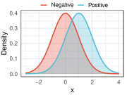
Refer to caption
Refer to caption
Refer to caption
Figure 3: Probability density functions of positive scores s+superscript𝑠s^{+} and negative scores ssuperscript𝑠s^{-}. Left: binormal (s𝒩(0,1),s+𝒩(1,1))formulae-sequencesimilar-tosuperscript𝑠𝒩01similar-tosuperscript𝑠𝒩11\left(s^{-}\sim\mathcal{N}(0,1),s^{+}\sim\mathcal{N}(1,1)\right). Middle: bibeta (s(2,5),s+(5,2))formulae-sequencesimilar-tosuperscript𝑠25similar-tosuperscript𝑠52\left(s^{-}\sim\mathcal{B}(2,5),s^{+}\sim\mathcal{B}(5,2)\right). Right: offset uniform (s𝒰(0,1),s+𝒰(0.5,1.5))formulae-sequencesimilar-tosuperscript𝑠𝒰01similar-tosuperscript𝑠𝒰0.51.5\left(s^{-}\sim\mathcal{U}(0,1),s^{+}\sim\mathcal{U}(0.5,1.5)\right).
Refer to captionRefer to captionRefer to caption
(a) π0=0.02subscript𝜋00.02\pi_{0}=0.02
Refer to captionRefer to captionRefer to caption
(b) π0=0.1subscript𝜋00.1\pi_{0}=0.1
Refer to captionRefer to captionRefer to caption
(c) π0=0.2subscript𝜋00.2\pi_{0}=0.2
Figure 4: Empirical analysis of estimation errors on simulation data. The score distributions of each row are binormal, bibeta and uniform offset in turn.
Refer to captionRefer to captionRefer to caption
(a) π0=0.01subscript𝜋00.01\pi_{0}=0.01
Refer to captionRefer to captionRefer to caption
(b) π0=0.03subscript𝜋00.03\pi_{0}=0.03
Refer to captionRefer to captionRefer to caption
(c) π0=0.1subscript𝜋00.1\pi_{0}=0.1
Figure 5: Empirical analysis of interpolation errors on simulation data. The score distributions of each row are binormal, bibeta and uniform offset in turn.

Appendix C Proofs on Generalization via Stability

C.1 Generalization by List Model Stability

See 1

Proof.

Let 𝒮,𝒮~𝒮~𝒮\mathcal{S},\widetilde{\mathcal{S}} be defined as in Def. 1. First of all, according to the symmetry, we have

𝔼𝒮,A[F(A(𝒮))F(A(𝒮);𝒮)]subscript𝔼𝒮𝐴delimited-[]𝐹𝐴𝒮𝐹𝐴𝒮𝒮\displaystyle\mathbb{E}_{\mathcal{S},A}[F(A(\mathcal{S}))-F(A(\mathcal{S});\mathcal{S})] (37)
=\displaystyle= 𝔼𝒮,𝒮~,A[F(A(𝒮);𝒮~)F(A(𝒮);𝒮)]subscript𝔼𝒮~𝒮𝐴delimited-[]𝐹𝐴𝒮~𝒮𝐹𝐴𝒮𝒮\displaystyle\mathbb{E}_{\mathcal{S},\widetilde{\mathcal{S}},A}[F(A(\mathcal{S});\widetilde{\mathcal{S}})-F(A(\mathcal{S});\mathcal{S})]
=\displaystyle= 𝔼𝒮,𝒮~,A[F(A(𝒮~);𝒮)F(A(𝒮);𝒮)]subscript𝔼𝒮~𝒮𝐴delimited-[]𝐹𝐴~𝒮𝒮𝐹𝐴𝒮𝒮\displaystyle\mathbb{E}_{\mathcal{S},\widetilde{\mathcal{S}},A}[F(A(\widetilde{\mathcal{S}});\mathcal{S})-F(A(\mathcal{S});\mathcal{S})]
=\displaystyle= 1M𝔼𝒮,𝒮~,A[𝒛𝒮(f^(A(𝒮~);𝒛)f^(A(𝒮);𝒛))]1𝑀subscript𝔼𝒮~𝒮𝐴delimited-[]subscriptsimilar-to𝒛𝒮^𝑓𝐴~𝒮𝒛^𝑓𝐴𝒮𝒛\displaystyle\frac{1}{M}\mathbb{E}_{\mathcal{S},\widetilde{\mathcal{S}},A}\left[\sum_{\bm{z}\sim\mathcal{S}}\left(\hat{f}(A(\widetilde{\mathcal{S}});\bm{z})-\hat{f}(A(\mathcal{S});\bm{z})\right)\right]
=\displaystyle= 𝔼𝒮,𝒮~,𝒛,𝒛~,A[f^(A((𝒮𝒛)𝒛~);𝒛)f^(A(𝒮);𝒛)],subscript𝔼𝒮~𝒮𝒛~𝒛𝐴delimited-[]^𝑓𝐴𝒮𝒛~𝒛𝒛^𝑓𝐴𝒮𝒛\displaystyle\mathbb{E}_{\mathcal{S},\widetilde{\mathcal{S}},\bm{z},\tilde{\bm{z}},A}\left[\hat{f}(A((\mathcal{S}-\bm{z})\cup\tilde{\bm{z}});\bm{z})-\hat{f}(A(\mathcal{S});\bm{z})\right],

where 𝒛𝒮𝒛𝒮\bm{z}\subseteq\mathcal{S} and 𝒛~𝒮~~𝒛~𝒮\tilde{\bm{z}}\subseteq\widetilde{\mathcal{S}}. Then, since the gradients of f^^𝑓\hat{f} is upper bounded by G𝐺G, we have

𝔼𝒮,𝒮~,𝒛,𝒛~,A[|f^(A((𝒮𝒛)𝒛~);𝒛)f^(A(𝒮);𝒛)|]subscript𝔼𝒮~𝒮𝒛~𝒛𝐴delimited-[]^𝑓𝐴𝒮𝒛~𝒛𝒛^𝑓𝐴𝒮𝒛\displaystyle\mathbb{E}_{\mathcal{S},\widetilde{\mathcal{S}},\bm{z},\tilde{\bm{z}},A}\left[\left|\hat{f}(A((\mathcal{S}-\bm{z})\cup\tilde{\bm{z}});\bm{z})-\hat{f}(A(\mathcal{S});\bm{z})\right|\right] (38)
\displaystyle\leq G𝔼𝒮,𝒮~,𝒛,𝒛~,A[A((𝒮𝒛)𝒛~)A(𝒮)2]𝐺subscript𝔼𝒮~𝒮𝒛~𝒛𝐴delimited-[]subscriptnorm𝐴𝒮𝒛~𝒛𝐴𝒮2\displaystyle G\cdot\mathbb{E}_{\mathcal{S},\widetilde{\mathcal{S}},\bm{z},\tilde{\bm{z}},A}\left[\left\|A((\mathcal{S}-\bm{z})\cup\tilde{\bm{z}})-A(\mathcal{S})\right\|_{2}\right]
\displaystyle\leq Gn+𝔼𝒮,𝒮(i),A[A(S(i))A(𝒮)2|yi=1]𝐺superscript𝑛subscript𝔼𝒮superscript𝒮𝑖𝐴delimited-[]conditionalsubscriptnorm𝐴superscript𝑆𝑖𝐴𝒮2subscript𝑦𝑖1\displaystyle Gn^{+}\cdot\mathbb{E}_{\mathcal{S},\mathcal{S}^{(i)},A}\left[\left\|A(S^{(i)})-A(\mathcal{S})\right\|_{2}\big{|}y_{i}=1\right]
+Gn𝔼𝒮,𝒮(i),A[A(S(i))A(𝒮)2|yi=1]𝐺superscript𝑛subscript𝔼𝒮superscript𝒮𝑖𝐴delimited-[]conditionalsubscriptnorm𝐴superscript𝑆𝑖𝐴𝒮2subscript𝑦𝑖1\displaystyle~{}~{}+Gn^{-}\cdot\mathbb{E}_{\mathcal{S},\mathcal{S}^{(i)},A}\left[\left\|A(S^{(i)})-A(\mathcal{S})\right\|_{2}\big{|}y_{i}=-1\right]
\displaystyle\leq Gn+N+𝔼𝒮,𝒮^,A[yi=1A(S(i))A(𝒮)2]+GnN𝔼𝒮,𝒮~,A[yi=1A(S(i))A(𝒮)2].𝐺superscript𝑛superscript𝑁subscript𝔼𝒮^𝒮𝐴delimited-[]subscriptsubscript𝑦𝑖1subscriptnorm𝐴superscript𝑆𝑖𝐴𝒮2𝐺superscript𝑛superscript𝑁subscript𝔼𝒮~𝒮𝐴delimited-[]subscriptsubscript𝑦𝑖1subscriptnorm𝐴superscript𝑆𝑖𝐴𝒮2\displaystyle\frac{Gn^{+}}{N^{+}}\mathbb{E}_{\mathcal{S},\widehat{\mathcal{S}},A}\left[\sum_{y_{i}=1}\left\|A(S^{(i)})-A(\mathcal{S})\right\|_{2}\right]+\frac{Gn^{-}}{N^{-}}\mathbb{E}_{\mathcal{S},\widetilde{\mathcal{S}},A}\left[\sum_{y_{i}=-1}\left\|A(S^{(i)})-A(\mathcal{S})\right\|_{2}\right].

The proof is completed by denoting

𝔼𝒮,𝒮~,A[1N+yi=1A(S(i))A(𝒮)2]=ϵ+,subscript𝔼𝒮~𝒮𝐴delimited-[]1superscript𝑁subscriptsubscript𝑦𝑖1subscriptnorm𝐴superscript𝑆𝑖𝐴𝒮2superscriptitalic-ϵ\displaystyle\mathbb{E}_{\mathcal{S},\widetilde{\mathcal{S}},A}\left[\frac{1}{N^{+}}\sum_{y_{i}=1}\left\|A(S^{(i)})-A(\mathcal{S})\right\|_{2}\right]=\epsilon^{+}, (39)
𝔼𝒮,𝒮~,A[1Nyi=1A(S(i))A(𝒮)2]=ϵ.subscript𝔼𝒮~𝒮𝐴delimited-[]1superscript𝑁subscriptsubscript𝑦𝑖1subscriptnorm𝐴superscript𝑆𝑖𝐴𝒮2superscriptitalic-ϵ\displaystyle\mathbb{E}_{\mathcal{S},\widetilde{\mathcal{S}},A}\left[\frac{1}{N^{-}}\sum_{y_{i}=-1}\left\|A(S^{(i)})-A(\mathcal{S})\right\|_{2}\right]=\epsilon^{-}.

C.2 List Model Stability of SOPRC

See 1

Proof.

For all i=1,,N𝑖1𝑁i=1,\cdots,N, let {𝒘t}t,{𝒗t}t,{𝒛it}tsubscriptsubscript𝒘𝑡𝑡subscriptsubscript𝒗𝑡𝑡subscriptsubscript𝒛subscript𝑖𝑡𝑡\{\bm{w}_{t}\}_{t},\{\bm{v}_{t}\}_{t},\{\bm{z}_{i_{t}}\}_{t} and {𝒘t}t,{𝒗t}t,{𝒛it}tsubscriptsubscriptsuperscript𝒘𝑡𝑡subscriptsubscriptsuperscript𝒗𝑡𝑡subscriptsubscriptsuperscript𝒛subscript𝑖𝑡𝑡\{\bm{w}^{\prime}_{t}\}_{t},\{\bm{v}^{\prime}_{t}\}_{t},\{\bm{z}^{\prime}_{i_{t}}\}_{t} be produced by Alg. 1 based on 𝒮𝒮\mathcal{S} and 𝒮(i)superscript𝒮𝑖\mathcal{S}^{(i)}, respectively. According to the update rules, for all t=1,,T𝑡1𝑇t=1,\cdots,T, we have

𝒘t+1𝒘t+12subscriptnormsubscriptsuperscript𝒘𝑡1subscript𝒘𝑡12\displaystyle\|\bm{w}^{\prime}_{t+1}-\bm{w}_{t+1}\|_{2} =𝒘t𝒘tηt(f(𝒘t;𝒛it,𝒗t+1)f(𝒘t;𝒛it,𝒗t+1))2absentsubscriptnormsubscriptsuperscript𝒘𝑡subscript𝒘𝑡subscript𝜂𝑡𝑓subscriptsuperscript𝒘𝑡subscriptsuperscript𝒛subscript𝑖𝑡subscriptsuperscript𝒗𝑡1𝑓subscript𝒘𝑡subscript𝒛subscript𝑖𝑡subscript𝒗𝑡12\displaystyle=\|\bm{w}^{\prime}_{t}-\bm{w}_{t}-\eta_{t}\left(\nabla f(\bm{w}^{\prime}_{t};\bm{z}^{\prime}_{i_{t}},\bm{v}^{\prime}_{t+1})-\nabla f(\bm{w}_{t};\bm{z}_{i_{t}},\bm{v}_{t+1})\right)\|_{2} (40)
𝒘t𝒘t2+ηtf(𝒘t;𝒛it,𝒗t+1)f(𝒘t;𝒛it,𝒗t+1)2.absentsubscriptnormsubscriptsuperscript𝒘𝑡subscript𝒘𝑡2subscript𝜂𝑡subscriptnorm𝑓subscriptsuperscript𝒘𝑡subscriptsuperscript𝒛subscript𝑖𝑡subscriptsuperscript𝒗𝑡1𝑓subscript𝒘𝑡subscript𝒛subscript𝑖𝑡subscript𝒗𝑡12\displaystyle\leq\|\bm{w}^{\prime}_{t}-\bm{w}_{t}\|_{2}+\eta_{t}\left\|\nabla f(\bm{w}^{\prime}_{t};\bm{z}^{\prime}_{i_{t}},\bm{v}^{\prime}_{t+1})-\nabla f(\bm{w}_{t};\bm{z}_{i_{t}},\bm{v}_{t+1})\right\|_{2}.

We discuss the second term on the right side in the following three cases.

Case 1: (𝒙i,yi)𝒛itsubscript𝒙𝑖subscript𝑦𝑖subscript𝒛subscript𝑖𝑡(\bm{x}_{i},y_{i})\notin\bm{z}_{i_{t}}. In this case, we have 𝒛it=𝒛itsubscript𝒛subscript𝑖𝑡subscriptsuperscript𝒛subscript𝑖𝑡\bm{z}_{i_{t}}=\bm{z}^{\prime}_{i_{t}}. According to the smoothness of f𝑓f and Lem. 4, we have

f(𝒘t;𝒛it,𝒗t+1)f(𝒘t;𝒛it,𝒗t+1)2subscriptnorm𝑓subscriptsuperscript𝒘𝑡subscriptsuperscript𝒛subscript𝑖𝑡subscriptsuperscript𝒗𝑡1𝑓subscript𝒘𝑡subscript𝒛subscript𝑖𝑡subscript𝒗𝑡12\displaystyle\left\|\nabla f(\bm{w}^{\prime}_{t};\bm{z}^{\prime}_{i_{t}},\bm{v}^{\prime}_{t+1})-\nabla f(\bm{w}_{t};\bm{z}_{i_{t}},\bm{v}_{t+1})\right\|_{2} (41)
\displaystyle\leq f(𝒘t;𝒛it,𝒗t+1)f(𝒘t;𝒛it,𝒗t+1)norm𝑓subscriptsuperscript𝒘𝑡subscript𝒛subscript𝑖𝑡subscriptsuperscript𝒗𝑡1𝑓subscript𝒘𝑡subscript𝒛subscript𝑖𝑡subscriptsuperscript𝒗𝑡1\displaystyle\left\|\nabla f(\bm{w}^{\prime}_{t};\bm{z}_{i_{t}},\bm{v}^{\prime}_{t+1})-\nabla f(\bm{w}_{t};\bm{z}_{i_{t}},\bm{v}^{\prime}_{t+1})\right\|
+f(𝒘t;𝒛it,𝒗t+1)f(𝒘t;𝒛it,𝒗t+1)2subscriptnorm𝑓subscript𝒘𝑡subscript𝒛subscript𝑖𝑡subscriptsuperscript𝒗𝑡1𝑓subscript𝒘𝑡subscript𝒛subscript𝑖𝑡subscript𝒗𝑡12\displaystyle~{}+\left\|\nabla f(\bm{w}_{t};\bm{z}_{i_{t}},\bm{v}^{\prime}_{t+1})-\nabla f(\bm{w}_{t};\bm{z}_{i_{t}},\bm{v}_{t+1})\right\|_{2}
\displaystyle\leq Lw𝒘t𝒘t2+Lv𝒗t+1𝒗t+12/N+,subscript𝐿𝑤subscriptnormsubscriptsuperscript𝒘𝑡subscript𝒘𝑡2subscript𝐿𝑣subscriptnormsubscriptsuperscript𝒗𝑡1subscript𝒗𝑡12superscript𝑁\displaystyle L_{w}\|\bm{w}^{\prime}_{t}-\bm{w}_{t}\|_{2}+L_{v}\|\bm{v}^{\prime}_{t+1}-\bm{v}_{t+1}\|_{2}/N^{+},

and

𝒗t+1𝒗t+12subscriptnormsubscriptsuperscript𝒗𝑡1subscript𝒗𝑡12\displaystyle\|\bm{v}^{\prime}_{t+1}-\bm{v}_{t+1}\|_{2} (42)
\displaystyle\leq (1βt)𝒗t𝒗t2+βtϕ(h𝒘t(𝒛it+))ϕ(h𝒘t(𝒛it+))21subscript𝛽𝑡subscriptnormsubscriptsuperscript𝒗𝑡subscript𝒗𝑡2subscript𝛽𝑡subscriptnormitalic-ϕsubscriptsubscriptsuperscript𝒘𝑡subscriptsuperscript𝒛subscript𝑖𝑡italic-ϕsubscriptsubscript𝒘𝑡subscriptsuperscript𝒛subscript𝑖𝑡2\displaystyle(1-\beta_{t})\|\bm{v}^{\prime}_{t}-\bm{v}_{t}\|_{2}+\beta_{t}\|\phi\left(h_{\bm{w}^{\prime}_{t}}(\bm{z}^{+}_{i_{t}})\right)-\phi\left(h_{\bm{w}_{t}}(\bm{z}^{+}_{i_{t}})\right)\|_{2}
\displaystyle\leq (1βt)𝒗t𝒗t2+CϕChβt𝒘t𝒘t21subscript𝛽𝑡subscriptnormsubscriptsuperscript𝒗𝑡subscript𝒗𝑡2subscript𝐶italic-ϕsubscript𝐶subscript𝛽𝑡subscriptnormsubscriptsuperscript𝒘𝑡subscript𝒘𝑡2\displaystyle(1-\beta_{t})\|\bm{v}^{\prime}_{t}-\bm{v}_{t}\|_{2}+C_{\phi}C_{h}\beta_{t}\|\bm{w}^{\prime}_{t}-\bm{w}_{t}\|_{2}
\displaystyle\leq (1βt)𝒗t𝒗t2+𝒘t𝒘t2/n+,1subscript𝛽𝑡subscriptnormsubscriptsuperscript𝒗𝑡subscript𝒗𝑡2subscriptnormsubscriptsuperscript𝒘𝑡subscript𝒘𝑡2superscript𝑛\displaystyle(1-\beta_{t})\|\bm{v}^{\prime}_{t}-\bm{v}_{t}\|_{2}+\|\bm{w}^{\prime}_{t}-\bm{w}_{t}\|_{2}/n^{+},

where the last inequation is due to βtCϕBn+subscript𝛽𝑡subscript𝐶italic-ϕ𝐵superscript𝑛\beta_{t}\leq\frac{C_{\phi}B}{n^{+}}.

Combining Eq. (40), Eq. (41) and Eq. (42), we have

𝒘t+1𝒘t+12subscriptnormsubscriptsuperscript𝒘𝑡1subscript𝒘𝑡12absent\displaystyle\|\bm{w}^{\prime}_{t+1}-\bm{w}_{t+1}\|_{2}\leq (1+Lwηt+Lvηt/n+)𝒘t𝒘t21subscript𝐿𝑤subscript𝜂𝑡subscript𝐿𝑣subscript𝜂𝑡superscript𝑛subscriptnormsubscriptsuperscript𝒘𝑡subscript𝒘𝑡2\displaystyle(1+L_{w}\eta_{t}+L_{v}\eta_{t}/n^{+})\|\bm{w}^{\prime}_{t}-\bm{w}_{t}\|_{2} (43)
+Lv(1βt)ηt𝒗t𝒗t2/N+subscript𝐿𝑣1subscript𝛽𝑡subscript𝜂𝑡subscriptnormsubscriptsuperscript𝒗𝑡subscript𝒗𝑡2superscript𝑁\displaystyle+L_{v}(1-\beta_{t})\eta_{t}\|\bm{v}^{\prime}_{t}-\bm{v}_{t}\|_{2}/N^{+}

Case 2: (𝒙i,yi)𝒛itsubscript𝒙𝑖subscript𝑦𝑖subscript𝒛subscript𝑖𝑡(\bm{x}_{i},y_{i})\in\bm{z}_{i_{t}} and yi=1subscript𝑦𝑖1y_{i}=1. In this case, we have 𝒛it=𝒛itsubscriptsuperscript𝒛subscript𝑖𝑡subscriptsuperscript𝒛subscript𝑖𝑡\bm{z}^{-}_{i_{t}}=\bm{z}^{\prime-}_{i_{t}}, thus

f(𝒘t;𝒛it,𝒗t+1)f(𝒘t;𝒛it,𝒗t+1)2subscriptnorm𝑓subscriptsuperscript𝒘𝑡subscriptsuperscript𝒛subscript𝑖𝑡subscriptsuperscript𝒗𝑡1𝑓subscript𝒘𝑡subscript𝒛subscript𝑖𝑡subscript𝒗𝑡12\displaystyle\left\|\nabla f(\bm{w}^{\prime}_{t};\bm{z}^{\prime}_{i_{t}},\bm{v}^{\prime}_{t+1})-\nabla f(\bm{w}_{t};\bm{z}_{i_{t}},\bm{v}_{t+1})\right\|_{2} (44)
\displaystyle\leq G/n++Lw𝒘t𝒘t2+Lv𝒗t+1𝒗t+12/N+,𝐺superscript𝑛subscript𝐿𝑤subscriptnormsubscriptsuperscript𝒘𝑡subscript𝒘𝑡2subscript𝐿𝑣subscriptnormsubscriptsuperscript𝒗𝑡1subscript𝒗𝑡12superscript𝑁\displaystyle G/n^{+}+L_{w}\|\bm{w}^{\prime}_{t}-\bm{w}_{t}\|_{2}+L_{v}\|\bm{v}^{\prime}_{t+1}-\bm{v}_{t+1}\|_{2}/N^{+},

and

𝒗t+1𝒗t+12subscriptnormsubscriptsuperscript𝒗𝑡1subscript𝒗𝑡12\displaystyle\|\bm{v}^{\prime}_{t+1}-\bm{v}_{t+1}\|_{2} (45)
\displaystyle\leq (1βt)𝒗t𝒗t2+βtϕ(h𝒘t(𝒛it+))ϕ(h𝒘t(𝒛it+))21subscript𝛽𝑡subscriptnormsubscriptsuperscript𝒗𝑡subscript𝒗𝑡2subscript𝛽𝑡subscriptnormitalic-ϕsubscriptsubscriptsuperscript𝒘𝑡subscriptsuperscript𝒛subscript𝑖𝑡italic-ϕsubscriptsubscript𝒘𝑡subscriptsuperscript𝒛subscript𝑖𝑡2\displaystyle(1-\beta_{t})\|\bm{v}^{\prime}_{t}-\bm{v}_{t}\|_{2}+\beta_{t}\|\phi\left(h_{\bm{w}^{\prime}_{t}}(\bm{z}^{\prime+}_{i_{t}})\right)-\phi\left(h_{\bm{w}_{t}}(\bm{z}^{\prime+}_{i_{t}})\right)\|_{2}
+βtϕ(h𝒘t(𝒛it+))ϕ(h𝒘t(𝒛it+))2subscript𝛽𝑡subscriptnormitalic-ϕsubscriptsubscript𝒘𝑡subscriptsuperscript𝒛subscript𝑖𝑡italic-ϕsubscriptsubscript𝒘𝑡subscriptsuperscript𝒛subscript𝑖𝑡2\displaystyle+\beta_{t}\|\phi\left(h_{\bm{w}_{t}}(\bm{z}^{\prime+}_{i_{t}})\right)-\phi\left(h_{\bm{w}_{t}}(\bm{z}^{+}_{i_{t}})\right)\|_{2}
\displaystyle\leq (1βt)𝒗t𝒗t2+𝒘t𝒘t2/n++2CϕBβt1subscript𝛽𝑡subscriptnormsubscriptsuperscript𝒗𝑡subscript𝒗𝑡2subscriptnormsubscriptsuperscript𝒘𝑡subscript𝒘𝑡2superscript𝑛2subscript𝐶italic-ϕ𝐵subscript𝛽𝑡\displaystyle(1-\beta_{t})\|\bm{v}^{\prime}_{t}-\bm{v}_{t}\|_{2}+\|\bm{w}^{\prime}_{t}-\bm{w}_{t}\|_{2}/n^{+}+2C_{\phi}B\beta_{t}
\displaystyle\leq (1βt)𝒗t𝒗t2+𝒘t𝒘t2/n++1/n+,1subscript𝛽𝑡subscriptnormsubscriptsuperscript𝒗𝑡subscript𝒗𝑡2subscriptnormsubscriptsuperscript𝒘𝑡subscript𝒘𝑡2superscript𝑛1superscript𝑛\displaystyle(1-\beta_{t})\|\bm{v}^{\prime}_{t}-\bm{v}_{t}\|_{2}+\|\bm{w}^{\prime}_{t}-\bm{w}_{t}\|_{2}/n^{+}+1/n^{+},

where the last inequality is due to βt2CϕB/n+subscript𝛽𝑡2subscript𝐶italic-ϕ𝐵superscript𝑛\beta_{t}\leq 2C_{\phi}B/n^{+}.

By combining Eq. (44) and Eq. (45), we have

𝒘t+1𝒘t+12subscriptnormsubscriptsuperscript𝒘𝑡1subscript𝒘𝑡12absent\displaystyle\|\bm{w}^{\prime}_{t+1}-\bm{w}_{t+1}\|_{2}\leq (1+Lwηt+Lvηt/n+)𝒘t𝒘t21subscript𝐿𝑤subscript𝜂𝑡subscript𝐿𝑣subscript𝜂𝑡superscript𝑛subscriptnormsubscriptsuperscript𝒘𝑡subscript𝒘𝑡2\displaystyle(1+L_{w}\eta_{t}+L_{v}\eta_{t}/n^{+})\|\bm{w}^{\prime}_{t}-\bm{w}_{t}\|_{2} (46)
+Lv(1βt)ηt𝒗t𝒗t2/N++(G+Lv/N+)ηt/n+.subscript𝐿𝑣1subscript𝛽𝑡subscript𝜂𝑡subscriptnormsubscriptsuperscript𝒗𝑡subscript𝒗𝑡2superscript𝑁𝐺subscript𝐿𝑣superscript𝑁subscript𝜂𝑡superscript𝑛\displaystyle+L_{v}(1-\beta_{t})\eta_{t}\|\bm{v}^{\prime}_{t}-\bm{v}_{t}\|_{2}/N^{+}+(G+L_{v}/N^{+})\eta_{t}/n^{+}.

Case 3: (𝒙i,yi)𝒛itsubscript𝒙𝑖subscript𝑦𝑖subscript𝒛subscript𝑖𝑡(\bm{x}_{i},y_{i})\in\bm{z}_{i_{t}} and yi=1subscript𝑦𝑖1y_{i}=-1. In this case, we have 𝒛it+=𝒛it+subscriptsuperscript𝒛subscript𝑖𝑡subscriptsuperscript𝒛subscript𝑖𝑡\bm{z}^{+}_{i_{t}}=\bm{z}^{\prime+}_{i_{t}}, thus

f(𝒘t;𝒛it,𝒗t+1)f(𝒘t;𝒛it,𝒗t+1)2subscriptnorm𝑓subscriptsuperscript𝒘𝑡subscriptsuperscript𝒛subscript𝑖𝑡subscriptsuperscript𝒗𝑡1𝑓subscript𝒘𝑡subscript𝒛subscript𝑖𝑡subscript𝒗𝑡12\displaystyle\left\|\nabla f(\bm{w}^{\prime}_{t};\bm{z}^{\prime}_{i_{t}},\bm{v}^{\prime}_{t+1})-\nabla f(\bm{w}_{t};\bm{z}_{i_{t}},\bm{v}_{t+1})\right\|_{2} (47)
\displaystyle\leq f(𝒘t;𝒛it,𝒗t+1)f(𝒘t;𝒛it,𝒗t+1)2subscriptnorm𝑓subscriptsuperscript𝒘𝑡subscriptsuperscript𝒛subscript𝑖𝑡subscriptsuperscript𝒗𝑡1𝑓subscriptsuperscript𝒘𝑡subscript𝒛subscript𝑖𝑡subscriptsuperscript𝒗𝑡12\displaystyle\left\|\nabla f(\bm{w}^{\prime}_{t};\bm{z}^{\prime}_{i_{t}},\bm{v}^{\prime}_{t+1})-\nabla f(\bm{w}^{\prime}_{t};\bm{z}_{i_{t}},\bm{v}^{\prime}_{t+1})\right\|_{2}
+f(𝒘t;𝒛it,𝒗t+1)f(𝒘t;𝒛it,𝒗t+1)2subscriptnorm𝑓subscriptsuperscript𝒘𝑡subscript𝒛subscript𝑖𝑡subscriptsuperscript𝒗𝑡1𝑓subscript𝒘𝑡subscript𝒛subscript𝑖𝑡subscriptsuperscript𝒗𝑡12\displaystyle~{}+\left\|\nabla f(\bm{w}^{\prime}_{t};\bm{z}_{i_{t}},\bm{v}^{\prime}_{t+1})-\nabla f(\bm{w}_{t};\bm{z}_{i_{t}},\bm{v}^{\prime}_{t+1})\right\|_{2}
+f(𝒘t;𝒛it,𝒗t+1)f(𝒘t;𝒛it,𝒗t+1)2subscriptnorm𝑓subscript𝒘𝑡subscript𝒛subscript𝑖𝑡subscriptsuperscript𝒗𝑡1𝑓subscript𝒘𝑡subscript𝒛subscript𝑖𝑡subscript𝒗𝑡12\displaystyle~{}+\left\|\nabla f(\bm{w}_{t};\bm{z}_{i_{t}},\bm{v}^{\prime}_{t+1})-\nabla f(\bm{w}_{t};\bm{z}_{i_{t}},\bm{v}_{t+1})\right\|_{2}
\displaystyle\leq Bn+/n+Lw𝒘t𝒘t2+Lv𝒗t+1𝒗t+12/N+,superscriptsubscript𝐵superscript𝑛superscript𝑛subscript𝐿𝑤subscriptnormsubscriptsuperscript𝒘𝑡subscript𝒘𝑡2subscript𝐿𝑣subscriptnormsubscriptsuperscript𝒗𝑡1subscript𝒗𝑡12superscript𝑁\displaystyle B_{\ell}^{\prime}\cdot n^{+}/n^{-}+L_{w}\|\bm{w}^{\prime}_{t}-\bm{w}_{t}\|_{2}+L_{v}\|\bm{v}^{\prime}_{t+1}-\bm{v}_{t+1}\|_{2}/N^{+},

where B=(1π)B/πsuperscriptsubscript𝐵1𝜋subscript𝐵𝜋B_{\ell}^{\prime}=(1-\pi)B_{\ell}/\pi. Similar to case 1, Eq. (42) still holds. Combining it with Eq. (47), we have

𝒘t+1𝒘t+12subscriptnormsubscriptsuperscript𝒘𝑡1subscript𝒘𝑡12absent\displaystyle\|\bm{w}^{\prime}_{t+1}-\bm{w}_{t+1}\|_{2}\leq (1+Lwηt+Lvηt/n+)𝒘t𝒘t21subscript𝐿𝑤subscript𝜂𝑡subscript𝐿𝑣subscript𝜂𝑡superscript𝑛subscriptnormsubscriptsuperscript𝒘𝑡subscript𝒘𝑡2\displaystyle(1+L_{w}\eta_{t}+L_{v}\eta_{t}/n^{+})\|\bm{w}^{\prime}_{t}-\bm{w}_{t}\|_{2} (48)
+Lvηt𝒗t𝒗t2/N++Bn+/nsubscript𝐿𝑣subscript𝜂𝑡subscriptnormsubscriptsuperscript𝒗𝑡subscript𝒗𝑡2superscript𝑁superscriptsubscript𝐵superscript𝑛superscript𝑛\displaystyle+L_{v}\eta_{t}\|\bm{v}^{\prime}_{t}-\bm{v}_{t}\|_{2}/N^{+}+B_{\ell}^{\prime}\cdot n^{+}/n^{-}

Next, we consider the expectation of 𝒘t+1𝒘t+12subscriptnormsubscriptsuperscript𝒘𝑡1subscript𝒘𝑡12\|\bm{w}^{\prime}_{t+1}-\bm{w}_{t+1}\|_{2} and 𝒗t+1𝒗t+12subscriptnormsubscriptsuperscript𝒗𝑡1subscript𝒗𝑡12\|\bm{v}^{\prime}_{t+1}-\bm{v}_{t+1}\|_{2} taking on A𝐴A. Note that

(case 1|yi=1)=(N+n+)/N+,conditionalcase 1subscript𝑦𝑖1superscript𝑁superscript𝑛superscript𝑁\displaystyle\mathbb{P}(\text{case 1}|y_{i}=1)=(N^{+}-n^{+})/N^{+}, (case 3|yi=1)=n+/N+,conditionalcase 3subscript𝑦𝑖1superscript𝑛superscript𝑁\displaystyle\mathbb{P}(\text{case 3}|y_{i}=1)=n^{+}/N^{+}, (49)
(case 1|yi=1)=(Nn)/N,conditionalcase 1subscript𝑦𝑖1superscript𝑁superscript𝑛superscript𝑁\displaystyle\mathbb{P}(\text{case 1}|y_{i}=-1)=(N^{-}-n^{-})/N^{-}, (case 2|yi=1)=n/N,conditionalcase 2subscript𝑦𝑖1superscript𝑛superscript𝑁\displaystyle\mathbb{P}(\text{case 2}|y_{i}=-1)=n^{-}/N^{-},

For yi=1subscript𝑦𝑖1y_{i}=1, we have

𝔼A[𝒘t+1𝒘t+12]subscript𝔼𝐴delimited-[]subscriptnormsubscriptsuperscript𝒘𝑡1subscript𝒘𝑡12absent\displaystyle\mathbb{E}_{A}\left[\|\bm{w}^{\prime}_{t+1}-\bm{w}_{t+1}\|_{2}\right]\leq (1+Lwηt+Lvηt/n+)𝔼A[𝒘t𝒘t2]1subscript𝐿𝑤subscript𝜂𝑡subscript𝐿𝑣subscript𝜂𝑡superscript𝑛subscript𝔼𝐴delimited-[]subscriptnormsubscriptsuperscript𝒘𝑡subscript𝒘𝑡2\displaystyle(1+L_{w}\eta_{t}+L_{v}\eta_{t}/n^{+})\mathbb{E}_{A}\left[\|\bm{w}^{\prime}_{t}-\bm{w}_{t}\|_{2}\right] (50)
+Lv(1βt)ηt𝔼A[𝒗t𝒗t2]/N++(G+Lv/N+)/N+,subscript𝐿𝑣1subscript𝛽𝑡subscript𝜂𝑡subscript𝔼𝐴delimited-[]subscriptnormsubscriptsuperscript𝒗𝑡subscript𝒗𝑡2superscript𝑁𝐺subscript𝐿𝑣superscript𝑁superscript𝑁\displaystyle+L_{v}(1-\beta_{t})\eta_{t}\mathbb{E}_{A}\left[\|\bm{v}^{\prime}_{t}-\bm{v}_{t}\|_{2}\right]/N^{+}+(G+L_{v}/N^{+})/N^{+},
𝔼A[𝒗t+1𝒗t+12]subscript𝔼𝐴delimited-[]subscriptnormsubscriptsuperscript𝒗𝑡1subscript𝒗𝑡12absent\displaystyle\mathbb{E}_{A}\left[\|\bm{v}^{\prime}_{t+1}-\bm{v}_{t+1}\|_{2}\right]\leq CϕBβt𝔼A[𝒘t𝒘t2]+𝔼A[𝒗t𝒗t2]+1/N+.subscript𝐶italic-ϕ𝐵subscript𝛽𝑡subscript𝔼𝐴delimited-[]subscriptnormsubscriptsuperscript𝒘𝑡subscript𝒘𝑡2subscript𝔼𝐴delimited-[]subscriptnormsubscriptsuperscript𝒗𝑡subscript𝒗𝑡21superscript𝑁\displaystyle C_{\phi}B\beta_{t}\mathbb{E}_{A}\left[\|\bm{w}^{\prime}_{t}-\bm{w}_{t}\|_{2}\right]+\mathbb{E}_{A}\left[\|\bm{v}^{\prime}_{t}-\bm{v}_{t}\|_{2}\right]+1/N^{+}.

By setting Lmax{Lw,Lv/n+,CϕB,G/2}𝐿subscript𝐿𝑤subscript𝐿𝑣superscript𝑛subscript𝐶italic-ϕ𝐵𝐺2L\geq\max\{L_{w},L_{v}/n^{+},C_{\phi}B,G/2\} and N+>2n+superscript𝑁2superscript𝑛N^{+}>2n^{+}, the above result can be rewritten as

[𝔼A[𝒘t+1𝒘t+12]𝔼A[𝒗t+1𝒗t+12]1]delimited-[]subscript𝔼𝐴delimited-[]subscriptnormsubscriptsuperscript𝒘𝑡1subscript𝒘𝑡12subscript𝔼𝐴delimited-[]subscriptnormsubscriptsuperscript𝒗𝑡1subscript𝒗𝑡121\displaystyle\left[\begin{array}[]{c}\mathbb{E}_{A}\left[\|\bm{w}^{\prime}_{t+1}-\bm{w}_{t+1}\|_{2}\right]\\ \mathbb{E}_{A}\left[\|\bm{v}^{\prime}_{t+1}-\bm{v}_{t+1}\|_{2}\right]\\ 1\end{array}\right] (51)
\displaystyle\leq [1+2LηtL(1βt)ηt/N+Lηt/N+Lβt11/N+001][𝔼A[𝒘t𝒘t2]𝔼A[𝒗t𝒗t2]1]delimited-[]12𝐿subscript𝜂𝑡𝐿1subscript𝛽𝑡subscript𝜂𝑡superscript𝑁𝐿subscript𝜂𝑡superscript𝑁𝐿subscript𝛽𝑡11superscript𝑁001delimited-[]subscript𝔼𝐴delimited-[]subscriptnormsubscriptsuperscript𝒘𝑡subscript𝒘𝑡2subscript𝔼𝐴delimited-[]subscriptnormsubscriptsuperscript𝒗𝑡subscript𝒗𝑡21\displaystyle\left[\begin{array}[]{ccc}1+2L\eta_{t}&L(1-\beta_{t})\eta_{t}/N^{+}&L\eta_{t}/N^{+}\\ L\beta_{t}&1&1/N^{+}\\ 0&0&1\end{array}\right]\left[\begin{array}[]{c}\mathbb{E}_{A}\left[\|\bm{w}^{\prime}_{t}-\bm{w}_{t}\|_{2}\right]\\ \mathbb{E}_{A}\left[\|\bm{v}^{\prime}_{t}-\bm{v}_{t}\|_{2}\right]\\ 1\end{array}\right]

Similarly, for yi=1subscript𝑦𝑖1y_{i}=-1, we have

𝔼A[𝒘t+1𝒘t+12]subscript𝔼𝐴delimited-[]subscriptnormsubscriptsuperscript𝒘𝑡1subscript𝒘𝑡12absent\displaystyle\mathbb{E}_{A}\left[\|\bm{w}^{\prime}_{t+1}-\bm{w}_{t+1}\|_{2}\right]\leq (1+Lwηt+Lvηt/n+)𝔼A[𝒘t𝒘t2]1subscript𝐿𝑤subscript𝜂𝑡subscript𝐿𝑣subscript𝜂𝑡superscript𝑛subscript𝔼𝐴delimited-[]subscriptnormsubscriptsuperscript𝒘𝑡subscript𝒘𝑡2\displaystyle(1+L_{w}\eta_{t}+L_{v}\eta_{t}/n^{+})\mathbb{E}_{A}\left[\|\bm{w}^{\prime}_{t}-\bm{w}_{t}\|_{2}\right] (52)
+Lv(1βt)ηt𝔼A[𝒗t𝒗t2]/N++Bn+/N,subscript𝐿𝑣1subscript𝛽𝑡subscript𝜂𝑡subscript𝔼𝐴delimited-[]subscriptnormsubscriptsuperscript𝒗𝑡subscript𝒗𝑡2superscript𝑁subscriptsuperscript𝐵superscript𝑛superscript𝑁\displaystyle+L_{v}(1-\beta_{t})\eta_{t}\mathbb{E}_{A}\left[\|\bm{v}^{\prime}_{t}-\bm{v}_{t}\|_{2}\right]/N^{+}+B^{\prime}_{\ell}n^{+}/N^{-},
𝔼A[𝒗t+1𝒗t+12]subscript𝔼𝐴delimited-[]subscriptnormsubscriptsuperscript𝒗𝑡1subscript𝒗𝑡12absent\displaystyle\mathbb{E}_{A}\left[\|\bm{v}^{\prime}_{t+1}-\bm{v}_{t+1}\|_{2}\right]\leq CϕBβt𝔼A[𝒘t𝒘t2]+𝔼A[𝒗t𝒗t2].subscript𝐶italic-ϕ𝐵subscript𝛽𝑡subscript𝔼𝐴delimited-[]subscriptnormsubscriptsuperscript𝒘𝑡subscript𝒘𝑡2subscript𝔼𝐴delimited-[]subscriptnormsubscriptsuperscript𝒗𝑡subscript𝒗𝑡2\displaystyle C_{\phi}B\beta_{t}\mathbb{E}_{A}\left[\|\bm{w}^{\prime}_{t}-\bm{w}_{t}\|_{2}\right]+\mathbb{E}_{A}\left[\|\bm{v}^{\prime}_{t}-\bm{v}_{t}\|_{2}\right].

By setting Lmax{Lw,Lv/n+,CϕB,G,B}𝐿subscript𝐿𝑤subscript𝐿𝑣superscript𝑛subscript𝐶italic-ϕ𝐵𝐺subscriptsuperscript𝐵L\geq\max\{L_{w},L_{v}/n^{+},C_{\phi}B,G,B^{\prime}_{\ell}\}, we have

[𝔼A[𝒘t+1𝒘t+12]𝔼A[𝒗t+1𝒗t+12]1]delimited-[]subscript𝔼𝐴delimited-[]subscriptnormsubscriptsuperscript𝒘𝑡1subscript𝒘𝑡12subscript𝔼𝐴delimited-[]subscriptnormsubscriptsuperscript𝒗𝑡1subscript𝒗𝑡121\displaystyle\left[\begin{array}[]{c}\mathbb{E}_{A}\left[\|\bm{w}^{\prime}_{t+1}-\bm{w}_{t+1}\|_{2}\right]\\ \mathbb{E}_{A}\left[\|\bm{v}^{\prime}_{t+1}-\bm{v}_{t+1}\|_{2}\right]\\ 1\end{array}\right] (53)
\displaystyle\leq [1+2LηtLv(1βt)ηt/NLηtn+/NLβt10001][𝔼A[𝒘t𝒘t2]𝔼A[𝒗t𝒗t2]1].delimited-[]12𝐿subscript𝜂𝑡subscript𝐿𝑣1subscript𝛽𝑡subscript𝜂𝑡superscript𝑁𝐿subscript𝜂𝑡superscript𝑛superscript𝑁𝐿subscript𝛽𝑡10001delimited-[]subscript𝔼𝐴delimited-[]subscriptnormsubscriptsuperscript𝒘𝑡subscript𝒘𝑡2subscript𝔼𝐴delimited-[]subscriptnormsubscriptsuperscript𝒗𝑡subscript𝒗𝑡21\displaystyle\left[\begin{array}[]{ccc}1+2L\eta_{t}&L_{v}(1-\beta_{t})\eta_{t}/N^{-}&L\eta_{t}\cdot n^{+}/N^{-}\\ L\beta_{t}&1&0\\ 0&0&1\end{array}\right]\left[\begin{array}[]{c}\mathbb{E}_{A}\left[\|\bm{w}^{\prime}_{t}-\bm{w}_{t}\|_{2}\right]\\ \mathbb{E}_{A}\left[\|\bm{v}^{\prime}_{t}-\bm{v}_{t}\|_{2}\right]\\ 1\end{array}\right].

Lemma 2.

Let 𝐳𝐳\bm{z}, 𝐳𝒵nsuperscript𝐳superscript𝒵𝑛\bm{z}^{\prime}\in\mathcal{Z}^{n} be two datasets that differ by exact one example and Asmp. 1 holds. For all 𝐰Ω,𝐯N+formulae-sequence𝐰Ω𝐯superscriptsuperscript𝑁\bm{w}\in\Omega,\bm{v}\in\mathbb{R}^{N^{+}}, the gradient difference of w.r.t. 𝐳𝐳\bm{z} and 𝐳superscript𝐳\bm{z}^{\prime} are upper bounded:

(a) If 𝐳,𝐳𝐳superscript𝐳\bm{z},\bm{z}^{\prime} differ by a negative example, then

f(𝒘;𝒛it,v)f(𝒘;𝒛it,v)2(1π)B|𝒛+|π|𝒛|subscriptnorm𝑓𝒘subscriptsuperscript𝒛subscript𝑖𝑡𝑣𝑓𝒘subscript𝒛subscript𝑖𝑡𝑣21𝜋subscript𝐵superscript𝒛𝜋superscript𝒛\displaystyle\|\nabla f(\bm{w};\bm{z}^{\prime}_{i_{t}},v)-\nabla f(\bm{w};\bm{z}_{i_{t}},v)\|_{2}\leq\frac{(1-\pi)B_{\ell}|\bm{z}^{+}|}{\pi|\bm{z}^{-}|} (54)

(b) If 𝐳,𝐳𝐳superscript𝐳\bm{z},\bm{z}^{\prime} differ by a positive example, then

f(𝒘;𝒛it,v)f(𝒘;𝒛it,v)2G/|𝒛+|subscriptnorm𝑓𝒘subscriptsuperscript𝒛subscript𝑖𝑡𝑣𝑓𝒘subscript𝒛subscript𝑖𝑡𝑣2𝐺superscript𝒛\displaystyle\|\nabla f(\bm{w};\bm{z}^{\prime}_{i_{t}},v)-\nabla f(\bm{w};\bm{z}_{i_{t}},v)\|_{2}\leq G/|\bm{z}^{+}| (55)
Proof.

The proof of (b) is obvious. For (a), let the different examples in 𝒛𝒛\bm{z} and 𝒛superscript𝒛\bm{z}^{\prime} be 𝒙~~𝒙\tilde{\bm{x}} and 𝒙~superscript~𝒙\tilde{\bm{x}}^{\prime}.

Denote c(𝒙;𝒗,)=𝔼^v𝒗[(h𝒘(𝒙)v))]c(\bm{x};\bm{v},\ell)=\hat{\mathbb{E}}_{v\sim\bm{v}}[\ell(h_{\bm{w}}(\bm{x})-v))], and rewrite f𝑓f as

f(𝒘;𝒛,𝒗)=𝔼^𝒙𝒛+[σ(1ππc(𝒙;h𝒘(𝒛),1)/c(𝒙;v,2))].𝑓𝒘𝒛𝒗subscript^𝔼𝒙superscript𝒛delimited-[]𝜎1𝜋𝜋𝑐𝒙subscript𝒘superscript𝒛subscript1𝑐𝒙𝑣subscript2f(\bm{w};\bm{z},\bm{v})=\hat{\mathbb{E}}_{\bm{x}\in\bm{z}^{+}}\left[\sigma\left(\frac{1-\pi}{\pi}\cdot c(\bm{x};h_{\bm{w}}(\bm{z}^{-}),\ell_{1})/c(\bm{x};v,\ell_{2})\right)\right]. (56)
f(𝒘;𝒛it,v)f(𝒘;𝒛it,v)2subscriptnorm𝑓𝒘subscriptsuperscript𝒛subscript𝑖𝑡𝑣𝑓𝒘subscript𝒛subscript𝑖𝑡𝑣2\displaystyle\|\nabla f(\bm{w};\bm{z}^{\prime}_{i_{t}},v)-\nabla f(\bm{w};\bm{z}_{i_{t}},v)\|_{2} (57)
\displaystyle\leq 𝔼^𝒙𝒛+[σ((1π)/πc(𝒙;h𝒘(𝒛),1)/c(𝒙;𝒗,2))\displaystyle\mathop{\hat{\mathbb{E}}}\limits_{\bm{x}\in\bm{z}^{+}}\left[\|\nabla\sigma\left((1-\pi)/\pi\cdot c(\bm{x};h_{\bm{w}}(\bm{z}^{-}),\ell_{1})/c(\bm{x};\bm{v},\ell_{2})\right)\right.
σ((1π)/πc(𝒙;h𝒘(𝒛),1)/c(𝒙;𝒗,2))2]\displaystyle-\left.\nabla\sigma\left((1-\pi)/\pi\cdot c(\bm{x};h_{\bm{w}}(\bm{z}^{\prime-}),\ell_{1})/c(\bm{x};\bm{v},\ell_{2})\right)\|_{2}\right]
\displaystyle\leq 𝔼^𝒙𝒛+[(1π)/πc(𝒙;h𝒘(𝒛),1)/c(𝒙;𝒗,2)\displaystyle\mathop{\hat{\mathbb{E}}}\limits_{\bm{x}\in\bm{z}^{+}}\left[\|(1-\pi)/\pi\cdot c(\bm{x};h_{\bm{w}}(\bm{z}^{-}),\ell_{1})/c(\bm{x};\bm{v},\ell_{2})\right.
(1π)/πc(𝒙;h𝒘(𝒛),1)/c(𝒙;𝒗,2)2]\displaystyle-\left.(1-\pi)/\pi\cdot c(\bm{x};h_{\bm{w}}(\bm{z}^{\prime-}),\ell_{1})/c(\bm{x};\bm{v},\ell_{2})\|_{2}\right]
\displaystyle\leq (1π)|𝒛+|π𝔼^𝒙𝒛+[c(𝒙;h𝒘(𝒛),1)c(𝒙;h𝒘(𝒛),1)2]1𝜋superscript𝒛𝜋subscript^𝔼𝒙superscript𝒛delimited-[]subscriptnorm𝑐𝒙subscript𝒘superscript𝒛subscript1𝑐𝒙subscript𝒘superscript𝒛subscript12\displaystyle\frac{(1-\pi)|\bm{z}^{+}|}{\pi}\mathop{\hat{\mathbb{E}}}\limits_{\bm{x}\in\bm{z}^{+}}\left[\|c(\bm{x};h_{\bm{w}}(\bm{z}^{-}),\ell_{1})-c(\bm{x};h_{\bm{w}}(\bm{z}^{\prime-}),\ell_{1})\|_{2}\right]
\displaystyle\leq (1π)B|𝒛+|π|𝒛|.1𝜋subscript𝐵superscript𝒛𝜋superscript𝒛\displaystyle\frac{(1-\pi)B_{\ell}|\bm{z}^{+}|}{\pi|\bm{z}^{-}|}.

Lemma 3.

For two datasets 𝒮,𝒮(i)𝒮superscript𝒮𝑖\mathcal{S},\mathcal{S}^{(i)} that differ by the i𝑖i-th element, let {𝐰t}t,{𝐯t}tsubscriptsubscript𝐰𝑡𝑡subscriptsubscript𝐯𝑡𝑡\{\bm{w}_{t}\}_{t},\{\bm{v}_{t}\}_{t} and {𝐰t}t,{𝐯t}tsubscriptsuperscriptsubscript𝐰𝑡𝑡subscriptsubscriptsuperscript𝐯𝑡𝑡\{\bm{w}_{t}^{\prime}\}_{t},\{\bm{v}^{\prime}_{t}\}_{t} be produced by Alg. 1 with 𝒮𝒮\mathcal{S} and 𝒮(i)superscript𝒮𝑖\mathcal{S}^{(i)}, respectively. If yi=1subscript𝑦𝑖1y_{i}=1, then for all t0[N+/n+]subscript𝑡0delimited-[]superscript𝑁superscript𝑛t_{0}\in[N^{+}/n^{+}] we have

𝔼𝒮,A[𝒎T+1(i)]t0n+N+[D(Ω)B1]+𝔼𝒮,A[𝒎T+1(i)|iIt0(A)],subscript𝔼𝒮𝐴delimited-[]superscriptsubscript𝒎𝑇1𝑖subscript𝑡0superscript𝑛superscript𝑁superscriptdelimited-[]𝐷Ω𝐵1topsubscript𝔼𝒮𝐴delimited-[]conditionalsuperscriptsubscript𝒎𝑇1𝑖𝑖subscript𝐼subscript𝑡0𝐴\begin{aligned} \mathbb{E}_{\mathcal{S},A}\left[\bm{m}_{T+1}^{(i)}\right]\leq\frac{t_{0}n^{+}}{N^{+}}\left[\begin{array}[]{ccc}D(\Omega)&B&1\end{array}\right]^{\top}+\mathbb{E}_{\mathcal{S},A}\left[\bm{m}_{T+1}^{(i)}~{}\big{|}~{}i\notin I_{t_{0}}(A)\right]\end{aligned}, (58)

where D(Ω)𝐷ΩD(\Omega) is the diameter of the hypothesis space, It(A):={𝐢1,,𝐢t}assignsubscript𝐼𝑡𝐴subscript𝐢1subscript𝐢𝑡I_{t}(A):=\{\bm{i}_{1},\cdots,\bm{i}_{t}\} is the set of indices selected by A𝐴A at the first t𝑡t-th iterations. Similarly, when yi=1subscript𝑦𝑖1y_{i}=-1, for all t0[N/n]subscript𝑡0delimited-[]superscript𝑁superscript𝑛t_{0}\in[N^{-}/n^{-}], we have

𝔼𝒮,A[𝒎T+1(i)]t0nN[D(Ω)B1]+𝔼𝒮,A[𝒎T+1(i)|iIt0(A)],subscript𝔼𝒮𝐴delimited-[]superscriptsubscript𝒎𝑇1𝑖subscript𝑡0superscript𝑛superscript𝑁superscriptdelimited-[]𝐷Ω𝐵1topsubscript𝔼𝒮𝐴delimited-[]conditionalsuperscriptsubscript𝒎𝑇1𝑖𝑖subscript𝐼subscript𝑡0𝐴\begin{aligned} \mathbb{E}_{\mathcal{S},A}\left[\bm{m}_{T+1}^{(i)}\right]\leq\frac{t_{0}n^{-}}{N^{-}}\left[\begin{array}[]{ccc}D(\Omega)&B&1\end{array}\right]^{\top}+\mathbb{E}_{\mathcal{S},A}\left[\bm{m}_{T+1}^{(i)}~{}\big{|}~{}i\notin I_{t_{0}}(A)\right]\end{aligned}, (59)
Proof.

Here we only need to prove the case yi=1subscript𝑦𝑖1y_{i}=1. According to the law of total probability, we have

𝔼𝒮,A[𝒎T+1(i)]subscript𝔼𝒮𝐴delimited-[]superscriptsubscript𝒎𝑇1𝑖absent\displaystyle\mathbb{E}_{\mathcal{S},A}\left[\bm{m}_{T+1}^{(i)}\right]\leq 𝔼𝒮,A[𝒎T+1(i)|iIt0(A)](iIt0(A))subscript𝔼𝒮𝐴delimited-[]conditionalsuperscriptsubscript𝒎𝑇1𝑖𝑖subscript𝐼subscript𝑡0𝐴𝑖subscript𝐼subscript𝑡0𝐴\displaystyle\mathbb{E}_{\mathcal{S},A}\left[\bm{m}_{T+1}^{(i)}~{}\big{|}~{}i\in I_{t_{0}}(A)\right]\mathbb{P}\left(i\in I_{t_{0}}(A)\right) (60)
+𝔼𝒮,A[𝒎t0(i)|iIT+1(A)](iIt0(A)).subscript𝔼𝒮𝐴delimited-[]conditionalsuperscriptsubscript𝒎subscript𝑡0𝑖𝑖subscript𝐼𝑇1𝐴𝑖subscript𝐼subscript𝑡0𝐴\displaystyle~{}~{}~{}~{}~{}~{}+\mathbb{E}_{\mathcal{S},A}\left[\bm{m}_{t_{0}}^{(i)}~{}\big{|}~{}i\notin I_{T+1}(A)\right]\mathbb{P}\left(i\notin I_{t_{0}}(A)\right).

Notice that

(iIt0(A))t=1t0(i𝒊t)=t0n+N+,𝑖subscript𝐼subscript𝑡0𝐴superscriptsubscript𝑡1subscript𝑡0𝑖subscript𝒊𝑡subscript𝑡0superscript𝑛superscript𝑁\mathbb{P}\left(i\in I_{t_{0}}(A)\right)\leq\sum_{t=1}^{t_{0}}\mathbb{P}\left(i\in\bm{i}_{t}\right)=\frac{t_{0}n^{+}}{N^{+}}, (61)

the proof is complete by bounding the first term on the right side of Eq. (60). ∎

See 2

Proof.

According to Lem. 1 and Lem. 3, we have

1N+yi=1𝔼𝒮,A[𝒎T+1(i)]1superscript𝑁subscriptsubscript𝑦𝑖1subscript𝔼𝒮𝐴delimited-[]subscriptsuperscript𝒎𝑖𝑇1absent\displaystyle\frac{1}{N^{+}}\sum_{y_{i}=1}\mathbb{E}_{\mathcal{S},A}\left[\bm{m}^{(i)}_{T+1}\right]\leq t0n+N+[D(Ω)B1]subscript𝑡0superscript𝑛superscript𝑁superscriptdelimited-[]𝐷Ω𝐵1top\displaystyle\frac{t_{0}n^{+}}{N^{+}}\left[\begin{array}[]{ccc}D(\Omega)&B&1\end{array}\right]^{\top} (62)
+t=t0T(𝑰3+𝑹t+)1N+yi=1𝔼𝒮,A[𝒎t0(i)|iIt0(A)]superscriptsubscriptproduct𝑡subscript𝑡0𝑇subscript𝑰3subscriptsuperscript𝑹𝑡1superscript𝑁subscriptsubscript𝑦𝑖1subscript𝔼𝒮𝐴delimited-[]conditionalsubscriptsuperscript𝒎𝑖subscript𝑡0𝑖subscript𝐼subscript𝑡0𝐴\displaystyle~{}~{}+\prod_{t=t_{0}}^{T}(\bm{I}_{3}+\bm{R}^{+}_{t})\cdot\frac{1}{N^{+}}\sum_{y_{i}=1}\mathbb{E}_{\mathcal{S},A}\left[\bm{m}^{(i)}_{t_{0}}\big{|}i\notin I_{t_{0}}(A)\right]
=\displaystyle= t0n+N+[D(Ω)B1]+t=t0T(𝑰3+𝑹t+)[001],subscript𝑡0superscript𝑛superscript𝑁superscriptdelimited-[]𝐷Ω𝐵1topsuperscriptsubscriptproduct𝑡subscript𝑡0𝑇subscript𝑰3subscriptsuperscript𝑹𝑡superscriptdelimited-[]001top\displaystyle\frac{t_{0}n^{+}}{N^{+}}\left[\begin{array}[]{ccc}D(\Omega)&B&1\end{array}\right]^{\top}+\prod_{t=t_{0}}^{T}(\bm{I}_{3}+\bm{R}^{+}_{t})\cdot\left[\begin{array}[]{ccc}0&0&1\end{array}\right]^{\top},

where the last equation is due to the fact that for all tt0𝑡subscript𝑡0t\leq t_{0}, 𝒛it=𝒛itsubscript𝒛subscript𝑖𝑡subscriptsuperscript𝒛subscript𝑖𝑡\bm{z}_{i_{t}}=\bm{z}^{\prime}_{i_{t}}, leading to 𝒘t=𝒘t,𝒗t=𝒗tformulae-sequencesubscript𝒘𝑡subscriptsuperscript𝒘𝑡subscript𝒗𝑡subscriptsuperscript𝒗𝑡\bm{w}_{t}=\bm{w}^{\prime}_{t},\bm{v}_{t}=\bm{v}^{\prime}_{t}.

Then we focus on t=t0T(𝑰3+𝑹t+)superscriptsubscriptproduct𝑡subscript𝑡0𝑇subscript𝑰3subscriptsuperscript𝑹𝑡\prod_{t=t_{0}}^{T}(\bm{I}_{3}+\bm{R}^{+}_{t}). Notice that all elements in this product are nonnegative, thus in the remainder of this proof, given two nonnegative matrics 𝒂,𝒃𝒂𝒃\bm{a},\bm{b} with the same shape, we say 𝒂𝒃𝒂𝒃\bm{a}\leq\bm{b} if all elements in 𝒂𝒂\bm{a} are not larger than that in 𝒃𝒃\bm{b}.

Denote

𝑴𝑴\displaystyle\bm{M} =LCη[2(1β)1/N+β01/N+000],absent𝐿subscript𝐶𝜂delimited-[]21𝛽1superscript𝑁𝛽01superscript𝑁000\displaystyle=LC_{\eta}\left[\begin{array}[]{ccc}2&(1-\beta)&1/N^{+}\\ \beta&0&1/N^{+}\\ 0&0&0\end{array}\right],

then by setting ηtCη/tsubscript𝜂𝑡subscript𝐶𝜂𝑡\eta_{t}\leq C_{\eta}/t we have

t=t0T(𝑰3+𝑹t+)superscriptsubscriptproduct𝑡subscript𝑡0𝑇subscript𝑰3subscriptsuperscript𝑹𝑡\displaystyle\prod_{t=t_{0}}^{T}(\bm{I}_{3}+\bm{R}^{+}_{t}) (63)
\displaystyle\leq t=t0T[1+2LηtLηt/N+LηtLβ11/N+001]superscriptsubscriptproduct𝑡subscript𝑡0𝑇delimited-[]12𝐿subscript𝜂𝑡𝐿subscript𝜂𝑡superscript𝑁𝐿subscript𝜂𝑡𝐿𝛽11superscript𝑁001\displaystyle\prod_{t=t_{0}}^{T}\left[\begin{array}[]{ccc}1+2L\eta_{t}&L\eta_{t}/N^{+}&L\eta_{t}\\ L\beta&1&1/N^{+}\\ 0&0&1\end{array}\right]
=\displaystyle= t=t0T[1+2LηtL(1β)ηtLηtLβN+1/N+001][10001/N+0001]superscriptsubscriptproduct𝑡subscript𝑡0𝑇delimited-[]12𝐿subscript𝜂𝑡𝐿1𝛽subscript𝜂𝑡𝐿subscript𝜂𝑡𝐿𝛽superscript𝑁1superscript𝑁001delimited-[]10001superscript𝑁0001\displaystyle\prod_{t=t_{0}}^{T}\left[\begin{array}[]{ccc}1+2L\eta_{t}&L(1-\beta)\eta_{t}&L\eta_{t}\\ L\beta&N^{+}&1/N^{+}\\ 0&0&1\end{array}\right]\left[\begin{array}[]{ccc}1&0&0\\ 0&1/N^{+}&0\\ 0&0&1\end{array}\right]
=\displaystyle= [1000N+0001]t=t0T([10001/N+0001][1+2LηtL(1β)ηtLηtLβN+1/N+001])[10001/N+0001]delimited-[]1000superscript𝑁0001superscriptsubscriptproduct𝑡subscript𝑡0𝑇delimited-[]10001superscript𝑁0001delimited-[]12𝐿subscript𝜂𝑡𝐿1𝛽subscript𝜂𝑡𝐿subscript𝜂𝑡𝐿𝛽superscript𝑁1superscript𝑁001delimited-[]10001superscript𝑁0001\displaystyle\left[\begin{array}[]{ccc}1&0&0\\ 0&N^{+}&0\\ 0&0&1\end{array}\right]\prod_{t=t_{0}}^{T}\left(\left[\begin{array}[]{ccc}1&0&0\\ 0&1/N^{+}&0\\ 0&0&1\end{array}\right]\left[\begin{array}[]{ccc}1+2L\eta_{t}&L(1-\beta)\eta_{t}&L\eta_{t}\\ L\beta&N^{+}&1/N^{+}\\ 0&0&1\end{array}\right]\right)\left[\begin{array}[]{ccc}1&0&0\\ 0&1/N^{+}&0\\ 0&0&1\end{array}\right]
=\displaystyle= [1000N+0001]t=t0T(𝑰3+[2LηtL(1β)ηtLηtLβ/N+01/(N+)2000])[10001/N+0001]delimited-[]1000superscript𝑁0001superscriptsubscriptproduct𝑡subscript𝑡0𝑇subscript𝑰3delimited-[]2𝐿subscript𝜂𝑡𝐿1𝛽subscript𝜂𝑡𝐿subscript𝜂𝑡𝐿𝛽superscript𝑁01superscriptsuperscript𝑁2000delimited-[]10001superscript𝑁0001\displaystyle\left[\begin{array}[]{ccc}1&0&0\\ 0&N^{+}&0\\ 0&0&1\end{array}\right]\prod_{t=t_{0}}^{T}\left(\bm{I}_{3}+\left[\begin{array}[]{ccc}2L\eta_{t}&L(1-\beta)\eta_{t}&L\eta_{t}\\ L\beta/N^{+}&0&1/(N^{+})^{2}\\ 0&0&0\end{array}\right]\right)\left[\begin{array}[]{ccc}1&0&0\\ 0&1/N^{+}&0\\ 0&0&1\end{array}\right]
\displaystyle\leq [1000N+0001]t=t0T(𝑰3+𝑴/t)[10001/N+0001],delimited-[]1000superscript𝑁0001superscriptsubscriptproduct𝑡subscript𝑡0𝑇subscript𝑰3𝑴𝑡delimited-[]10001superscript𝑁0001\displaystyle\left[\begin{array}[]{ccc}1&0&0\\ 0&N^{+}&0\\ 0&0&1\end{array}\right]\prod_{t=t_{0}}^{T}\left(\bm{I}_{3}+\bm{M}/t\right)\left[\begin{array}[]{ccc}1&0&0\\ 0&1/N^{+}&0\\ 0&0&1\end{array}\right],

where the last inequation is due to N+Tsuperscript𝑁𝑇N^{+}\geq T. Notice that 𝑴𝟎3×3𝑴subscript033\bm{M}\geq\bm{0}_{3\times 3}, thus we have

t=t0T(𝑰3+𝑴/t)superscriptsubscriptproduct𝑡subscript𝑡0𝑇subscript𝑰3𝑴𝑡absent\displaystyle\prod_{t=t_{0}}^{T}\left(\bm{I}_{3}+\bm{M}/t\right)\leq t=t0Texp(𝑴/t)superscriptsubscriptproduct𝑡subscript𝑡0𝑇𝑴𝑡\displaystyle\prod_{t=t_{0}}^{T}\exp(\bm{M}/t) (64)
=\displaystyle= exp(t=t0T𝑴/t)superscriptsubscript𝑡subscript𝑡0𝑇𝑴𝑡\displaystyle\exp\left(\sum_{t=t_{0}}^{T}\bm{M}/t\right)
\displaystyle\leq exp(𝑴log(T/(t01)))𝑴𝑇subscript𝑡01\displaystyle\exp\left(\bm{M}\log(T/(t_{0}-1))\right)
=\displaystyle= Λdiag((Tt01)λ1,(Tt01)λ2,(Tt01)λ3)Λ1,Λ𝑑𝑖𝑎𝑔superscript𝑇subscript𝑡01subscript𝜆1superscript𝑇subscript𝑡01subscript𝜆2superscript𝑇subscript𝑡01subscript𝜆3superscriptΛ1\displaystyle\Lambda~{}diag\left(\left(\frac{T}{t_{0}-1}\right)^{\lambda_{1}},\left(\frac{T}{t_{0}-1}\right)^{\lambda_{2}},\left(\frac{T}{t_{0}-1}\right)^{\lambda_{3}}\right)\Lambda^{-1},

where the last eqution is obtained by diagonalizing 𝑴𝑴\bm{M} into Λdiag(λ1,λ2,λ3)Λ1Λ𝑑𝑖𝑎𝑔subscript𝜆1subscript𝜆2subscript𝜆3superscriptΛ1\Lambda~{}diag(\lambda_{1},\lambda_{2},\lambda_{3})\Lambda^{-1}, λisubscript𝜆𝑖\lambda_{i} are the eigenvalues of 𝑴𝑴\bm{M} and the columns of ΛΛ\Lambda are the corresponding eigen vectors.

Combining Eq. (63) and Eq. (64), we have

[100]t=t0T(𝑰3+𝑹t+)[001]delimited-[]100superscriptsubscriptproduct𝑡subscript𝑡0𝑇subscript𝑰3subscriptsuperscript𝑹𝑡superscriptdelimited-[]001top\displaystyle\left[\begin{array}[]{ccc}1&0&0\end{array}\right]\prod_{t=t_{0}}^{T}(\bm{I}_{3}+\bm{R}^{+}_{t})\left[\begin{array}[]{ccc}0&0&1\end{array}\right]^{\top} (65)
\displaystyle\leq [100][1000N+0001]t=t0T(𝑰3+𝑴/t)[10001/N+0001][001]delimited-[]100delimited-[]1000superscript𝑁0001superscriptsubscriptproduct𝑡subscript𝑡0𝑇subscript𝑰3𝑴𝑡delimited-[]10001superscript𝑁0001delimited-[]001\displaystyle\left[\begin{array}[]{ccc}1&0&0\end{array}\right]\left[\begin{array}[]{ccc}1&0&0\\ 0&N^{+}&0\\ 0&0&1\end{array}\right]\prod_{t=t_{0}}^{T}\left(\bm{I}_{3}+\bm{M}/t\right)\left[\begin{array}[]{ccc}1&0&0\\ 0&1/N^{+}&0\\ 0&0&1\end{array}\right]\left[\begin{array}[]{c}0\\ 0\\ 1\end{array}\right]
\displaystyle\leq [100]t=t0T(𝑰3+𝑴/t)[001]delimited-[]100superscriptsubscriptproduct𝑡subscript𝑡0𝑇subscript𝑰3𝑴𝑡delimited-[]001\displaystyle\left[\begin{array}[]{ccc}1&0&0\end{array}\right]\prod_{t=t_{0}}^{T}\left(\bm{I}_{3}+\bm{M}/t\right)\left[\begin{array}[]{c}0\\ 0\\ 1\end{array}\right]
\displaystyle\leq [100]Λdiag((Tt01)λ1,(Tt01)λ2,(Tt01)λ3)Λ1[001].delimited-[]100Λ𝑑𝑖𝑎𝑔superscript𝑇subscript𝑡01subscript𝜆1superscript𝑇subscript𝑡01subscript𝜆2superscript𝑇subscript𝑡01subscript𝜆3superscriptΛ1delimited-[]001\displaystyle\left[\begin{array}[]{ccc}1&0&0\end{array}\right]\Lambda~{}diag\left(\left(\frac{T}{t_{0}-1}\right)^{\lambda_{1}},\left(\frac{T}{t_{0}-1}\right)^{\lambda_{2}},\left(\frac{T}{t_{0}-1}\right)^{\lambda_{3}}\right)\Lambda^{-1}\left[\begin{array}[]{c}0\\ 0\\ 1\end{array}\right].

Specifically, we have λ1,2=LCη(1±1+ββ2),λ3=0formulae-sequencesubscript𝜆12𝐿subscript𝐶𝜂plus-or-minus11𝛽superscript𝛽2subscript𝜆30\lambda_{1,2}=LC_{\eta}(1\pm\sqrt{1+\beta-\beta^{2}}),\lambda_{3}=0, and

Λ=[111βN+β(11+ββ2)1ββ(1+1+ββ2)1β2+ββ(1β)N+001],Λdelimited-[]111𝛽superscript𝑁𝛽11𝛽superscript𝛽21𝛽𝛽11𝛽superscript𝛽21𝛽2𝛽𝛽1𝛽superscript𝑁001\Lambda=\left[\begin{array}[]{ccc}1&1&\frac{1}{\beta N^{+}}\\ \frac{\beta(1-\sqrt{1+\beta-\beta^{2}})}{1-\beta}&\frac{\beta(1+\sqrt{1+\beta-\beta^{2}})}{1-\beta}&-\frac{2+\beta}{\beta(1-\beta)N^{+}}\\ 0&0&-1\end{array}\right], (66)

leading to

[100]Λ=[111βN+],delimited-[]100Λdelimited-[]111𝛽superscript𝑁\left[\begin{array}[]{ccc}1&0&0\end{array}\right]\Lambda=\left[\begin{array}[]{ccc}1&1&\frac{1}{\beta N^{+}}\end{array}\right], (67)
Λ1[001]=[2+2β+β1+ββ22β21+ββ2N+22β+β1+ββ22β21+ββ2N+1],superscriptΛ1superscriptdelimited-[]001topsuperscriptdelimited-[]22𝛽𝛽1𝛽superscript𝛽22superscript𝛽21𝛽superscript𝛽2superscript𝑁22𝛽𝛽1𝛽superscript𝛽22superscript𝛽21𝛽superscript𝛽2superscript𝑁1top\Lambda^{-1}\left[\begin{array}[]{c}0\\ 0\\ 1\end{array}\right]^{\top}=\left[\begin{array}[]{c}\frac{2+2\beta+\beta\sqrt{1+\beta-\beta^{2}}}{2\beta^{2}\sqrt{1+\beta-\beta^{2}}N^{+}}\\ \frac{-2-2\beta+\beta\sqrt{1+\beta-\beta^{2}}}{2\beta^{2}\sqrt{1+\beta-\beta^{2}}N^{+}}\\ -1\end{array}\right]^{\top}, (68)
[100]Λdiag((Tt01)λ1,(Tt01)λ2,(Tt01)λ3)Λ1[001]delimited-[]100Λ𝑑𝑖𝑎𝑔superscript𝑇subscript𝑡01subscript𝜆1superscript𝑇subscript𝑡01subscript𝜆2superscript𝑇subscript𝑡01subscript𝜆3superscriptΛ1delimited-[]001\displaystyle\left[\begin{array}[]{ccc}1&0&0\end{array}\right]\Lambda~{}diag\left(\left(\frac{T}{t_{0}-1}\right)^{\lambda_{1}},\left(\frac{T}{t_{0}-1}\right)^{\lambda_{2}},\left(\frac{T}{t_{0}-1}\right)^{\lambda_{3}}\right)\Lambda^{-1}\left[\begin{array}[]{c}0\\ 0\\ 1\end{array}\right] (69)
=\displaystyle= 2+2β+β1+ββ22β21+ββ2Tλ1(t01)λ1N+22𝛽𝛽1𝛽superscript𝛽22superscript𝛽21𝛽superscript𝛽2superscript𝑇subscript𝜆1superscriptsubscript𝑡01subscript𝜆1superscript𝑁\displaystyle\frac{2+2\beta+\beta\sqrt{1+\beta-\beta^{2}}}{2\beta^{2}\sqrt{1+\beta-\beta^{2}}}\cdot\frac{T^{\lambda_{1}}}{(t_{0}-1)^{\lambda_{1}}N^{+}}
+22β+β1+ββ22β21+ββ2N+Tλ2(t01)λ2N+22𝛽𝛽1𝛽superscript𝛽22superscript𝛽21𝛽superscript𝛽2superscript𝑁superscript𝑇subscript𝜆2superscriptsubscript𝑡01subscript𝜆2superscript𝑁\displaystyle~{}~{}+\frac{-2-2\beta+\beta\sqrt{1+\beta-\beta^{2}}}{2\beta^{2}\sqrt{1+\beta-\beta^{2}}N^{+}}\cdot\frac{T^{\lambda_{2}}}{(t_{0}-1)^{\lambda_{2}}N^{+}}
Tλ2β(t01)λ2N+superscript𝑇subscript𝜆2𝛽superscriptsubscript𝑡01subscript𝜆2superscript𝑁\displaystyle~{}~{}-\frac{T^{\lambda_{2}}}{\beta(t_{0}-1)^{\lambda_{2}}N^{+}}
\displaystyle\leq 1+2ββ2Tλ1(t01)λ1N+12𝛽superscript𝛽2superscript𝑇subscript𝜆1superscriptsubscript𝑡01subscript𝜆1superscript𝑁\displaystyle\frac{1+2\beta}{\beta^{2}}\cdot\frac{T^{\lambda_{1}}}{(t_{0}-1)^{\lambda_{1}}N^{+}}

Combining Eq. (62), Eq. (65), Eq. (69), we have

1N+yi=1𝔼𝒮,A[𝒘T+1𝒘T+1(i)2]=𝒪((T/t0)λ1/N++t0n+N+),1superscript𝑁subscriptsubscript𝑦𝑖1subscript𝔼𝒮𝐴delimited-[]subscriptnormsubscript𝒘𝑇1superscriptsubscript𝒘𝑇1𝑖2𝒪superscript𝑇subscript𝑡0subscript𝜆1superscript𝑁subscript𝑡0superscript𝑛superscript𝑁\frac{1}{N^{+}}\sum_{y_{i}=1}\mathbb{E}_{\mathcal{S},A}\left[\|\bm{w}_{T+1}-\bm{w}_{T+1}^{(i)}\|_{2}\right]=\mathcal{O}\left((T/t_{0})^{\lambda_{1}}/N^{+}+\frac{t_{0}n^{+}}{N^{+}}\right), (70)

by choosing t0Tλ1λ1+1(n+)1λ1+1asymptotically-equalssubscript𝑡0superscript𝑇subscript𝜆1subscript𝜆11superscriptsuperscript𝑛1subscript𝜆11t_{0}\asymp T^{\frac{\lambda_{1}}{\lambda_{1}+1}}\cdot(n^{+})^{-\frac{1}{\lambda_{1}+1}}, we have

1N+yi=1𝔼𝒮,A[𝒘T+1𝒘T+1(i)2]=𝒪(Tλ1λ1+1(n+)λ1λ1+1N+).1superscript𝑁subscriptsubscript𝑦𝑖1subscript𝔼𝒮𝐴delimited-[]subscriptnormsubscript𝒘𝑇1superscriptsubscript𝒘𝑇1𝑖2𝒪superscript𝑇subscript𝜆1subscript𝜆11superscriptsuperscript𝑛subscript𝜆1subscript𝜆11superscript𝑁\frac{1}{N^{+}}\sum_{y_{i}=1}\mathbb{E}_{\mathcal{S},A}\left[\|\bm{w}_{T+1}-\bm{w}_{T+1}^{(i)}\|_{2}\right]=\mathcal{O}\left(\frac{T^{\frac{\lambda_{1}}{\lambda_{1}+1}}\cdot(n^{+})^{\frac{\lambda_{1}}{\lambda_{1}+1}}}{N^{+}}\right). (71)

Similarly, for yi=1subscript𝑦𝑖1y_{i}=-1, let

𝑴superscript𝑴\displaystyle\bm{M}^{\prime} =LCη[2(1β)1/Nβ01/N000],absent𝐿subscript𝐶𝜂delimited-[]21𝛽1superscript𝑁𝛽01superscript𝑁000\displaystyle=LC_{\eta}\left[\begin{array}[]{ccc}2&(1-\beta)&1/N^{-}\\ \beta&0&1/N^{-}\\ 0&0&0\end{array}\right],

which shares the same eigenvalues with 𝑴𝑴\bm{M}, thus we have

1Nyi=1𝔼𝒮,A[𝒘T+1𝒘T+1(i)2]=𝒪(Tλ1λ1+1(n)λ1λ1+1N).1superscript𝑁subscriptsubscript𝑦𝑖1subscript𝔼𝒮𝐴delimited-[]subscriptnormsubscript𝒘𝑇1superscriptsubscript𝒘𝑇1𝑖2𝒪superscript𝑇subscript𝜆1subscript𝜆11superscriptsuperscript𝑛subscript𝜆1subscript𝜆11superscript𝑁\frac{1}{N^{-}}\sum_{y_{i}=-1}\mathbb{E}_{\mathcal{S},A}\left[\|\bm{w}_{T+1}-\bm{w}_{T+1}^{(i)}\|_{2}\right]=\mathcal{O}\left(\frac{T^{\frac{\lambda_{1}}{\lambda_{1}+1}}\cdot(n^{-})^{\frac{\lambda_{1}}{\lambda_{1}+1}}}{N^{-}}\right). (72)

C.3 Convergence Rate

See 3

Proof.

First, according to the recurrence of 𝒗tsubscript𝒗𝑡\bm{v}_{t}, we have

𝒗t+1=τ=1t(1β)tτβϕ(h𝒘τ(𝒛iτ)).subscript𝒗𝑡1superscriptsubscript𝜏1𝑡superscript1𝛽𝑡𝜏𝛽italic-ϕsubscriptsubscript𝒘𝜏subscript𝒛subscript𝑖𝜏\bm{v}_{t+1}=\sum_{\tau=1}^{t}(1-\beta)^{t-\tau}\beta\cdot\phi\left(h_{\bm{w}_{\tau}}(\bm{z}_{i_{\tau}})\right). (73)

For sake of the presentation, denote

𝒖t+1subscript𝒖𝑡1\displaystyle\bm{u}_{t+1} =τ=1t(1β)tτβh𝒘τ(𝒮+)absentsuperscriptsubscript𝜏1𝑡superscript1𝛽𝑡𝜏𝛽subscriptsubscript𝒘𝜏superscript𝒮\displaystyle=\sum_{\tau=1}^{t}(1-\beta)^{t-\tau}\beta\cdot h_{\bm{w}_{\tau}}(\mathcal{S}^{+}) (74)
𝒈tsubscript𝒈𝑡\displaystyle\bm{g}_{t} =𝔼𝒮[f(𝒘t;𝒛it,𝒗t+1)]absentsubscript𝔼𝒮delimited-[]𝑓subscript𝒘𝑡subscript𝒛subscript𝑖𝑡subscript𝒗𝑡1\displaystyle=\mathbb{E}_{\mathcal{S}}[\nabla f\left(\bm{w}_{t};\bm{z}_{i_{t}},\bm{v}_{t+1}\right)]
δ1tsuperscriptsubscript𝛿1𝑡\displaystyle\delta_{1}^{t} =F(𝒘t)𝔼𝒮[f(𝒘t;𝒛it,h𝒘t(𝒮+))]absent𝐹subscript𝒘𝑡subscript𝔼𝒮delimited-[]𝑓subscript𝒘𝑡subscript𝒛subscript𝑖𝑡subscriptsubscript𝒘𝑡superscript𝒮\displaystyle=\nabla F(\bm{w}_{t})-\mathbb{E}_{\mathcal{S}}\left[\nabla f\left(\bm{w}_{t};\bm{z}_{i_{t}},h_{\bm{w}_{t}}(\mathcal{S}^{+})\right)\right]
δ2tsuperscriptsubscript𝛿2𝑡\displaystyle\delta_{2}^{t} =𝔼𝒮[f(𝒘t;𝒛it,h𝒘t(𝒮+))f(𝒘t;𝒛it,𝒖t+1)]absentsubscript𝔼𝒮delimited-[]𝑓subscript𝒘𝑡subscript𝒛subscript𝑖𝑡subscriptsubscript𝒘𝑡superscript𝒮𝑓subscript𝒘𝑡subscript𝒛subscript𝑖𝑡subscript𝒖𝑡1\displaystyle=\mathbb{E}_{\mathcal{S}}\left[\nabla f\left(\bm{w}_{t};\bm{z}_{i_{t}},h_{\bm{w}_{t}}(\mathcal{S}^{+})\right)-\nabla f\left(\bm{w}_{t};\bm{z}_{i_{t}},\bm{u}_{t+1}\right)\right]
δ3tsuperscriptsubscript𝛿3𝑡\displaystyle\delta_{3}^{t} =𝔼𝒮[f(𝒘t;𝒛it,𝒖t+1)f(𝒘t;𝒛it,𝒗t+1)].absentsubscript𝔼𝒮delimited-[]𝑓subscript𝒘𝑡subscript𝒛subscript𝑖𝑡subscript𝒖𝑡1𝑓subscript𝒘𝑡subscript𝒛subscript𝑖𝑡subscript𝒗𝑡1\displaystyle=\mathbb{E}_{\mathcal{S}}\left[\nabla f\left(\bm{w}_{t};\bm{z}_{i_{t}},\bm{u}_{t+1}\right)-\nabla f\left(\bm{w}_{t};\bm{z}_{i_{t}},\bm{v}_{t+1}\right)\right].

According to the smoothness of F𝐹F, we have

F(𝒘t+1)𝐹subscript𝒘𝑡1absent\displaystyle F(\bm{w}_{t+1})\leq F(𝒘t)+F(𝒘t),𝒙t+1𝒙t+Lw2𝒙t+1𝒙t22𝐹subscript𝒘𝑡𝐹subscript𝒘𝑡subscript𝒙𝑡1subscript𝒙𝑡subscript𝐿𝑤2superscriptsubscriptnormsubscript𝒙𝑡1subscript𝒙𝑡22\displaystyle F(\bm{w}_{t})+\langle\nabla F(\bm{w}_{t}),\bm{x}_{t+1}-\bm{x}_{t}\rangle+\frac{L_{w}}{2}\|\bm{x}_{t+1}-\bm{x}_{t}\|_{2}^{2} (75)
=\displaystyle= F(𝒘t)ηtF(𝒘t),𝒈t+Lwηt22𝒈t22𝐹subscript𝒘𝑡subscript𝜂𝑡𝐹subscript𝒘𝑡subscript𝒈𝑡subscript𝐿𝑤superscriptsubscript𝜂𝑡22superscriptsubscriptnormsubscript𝒈𝑡22\displaystyle F(\bm{w}_{t})-\eta_{t}\langle\nabla F(\bm{w}_{t}),\bm{g}_{t}\rangle+\frac{L_{w}\eta_{t}^{2}}{2}\|\bm{g}_{t}\|_{2}^{2}
=\displaystyle= F(𝒘t)ηtF(𝒘t)22+ηtF(𝒘t),δ1t+δ2t+δ3t+Lwηt22𝒈t22.𝐹subscript𝒘𝑡subscript𝜂𝑡superscriptsubscriptnorm𝐹subscript𝒘𝑡22subscript𝜂𝑡𝐹subscript𝒘𝑡superscriptsubscript𝛿1𝑡superscriptsubscript𝛿2𝑡superscriptsubscript𝛿3𝑡subscript𝐿𝑤superscriptsubscript𝜂𝑡22superscriptsubscriptnormsubscript𝒈𝑡22\displaystyle F(\bm{w}_{t})-\eta_{t}\|\nabla F(\bm{w}_{t})\|_{2}^{2}+\eta_{t}\langle\nabla F(\bm{w}_{t}),\delta_{1}^{t}+\delta_{2}^{t}+\delta_{3}^{t}\rangle+\frac{L_{w}\eta_{t}^{2}}{2}\|\bm{g}_{t}\|_{2}^{2}.

By taking expectation of A𝐴A on both sides, we have

𝔼A[F(𝒘t+1)]subscript𝔼𝐴delimited-[]𝐹subscript𝒘𝑡1absent\displaystyle\mathbb{E}_{A}[F(\bm{w}_{t+1})]\leq 𝔼A[F(𝒘t)]ηt𝔼A[F(𝒘t)22]+Lwηt22𝔼A[𝒈t22]subscript𝔼𝐴delimited-[]𝐹subscript𝒘𝑡subscript𝜂𝑡subscript𝔼𝐴delimited-[]superscriptsubscriptnorm𝐹subscript𝒘𝑡22subscript𝐿𝑤superscriptsubscript𝜂𝑡22subscript𝔼𝐴delimited-[]superscriptsubscriptnormsubscript𝒈𝑡22\displaystyle\mathbb{E}_{A}[F(\bm{w}_{t})]-\eta_{t}\mathbb{E}_{A}[\|\nabla F(\bm{w}_{t})\|_{2}^{2}]+\frac{L_{w}\eta_{t}^{2}}{2}\mathbb{E}_{A}\left[\|\bm{g}_{t}\|_{2}^{2}\right] (76)
+ηt𝔼A[F(𝒘t),δ2t+δ3t]subscript𝜂𝑡subscript𝔼𝐴delimited-[]𝐹subscript𝒘𝑡superscriptsubscript𝛿2𝑡superscriptsubscript𝛿3𝑡\displaystyle+\eta_{t}\mathbb{E}_{A}\left[\langle\nabla F(\bm{w}_{t}),\delta_{2}^{t}+\delta_{3}^{t}\rangle\right]
\displaystyle\leq 𝔼A[F(𝒘t)]ηt𝔼A[F(𝒘t)22]+Lwηt22𝔼A[𝒈t22]subscript𝔼𝐴delimited-[]𝐹subscript𝒘𝑡subscript𝜂𝑡subscript𝔼𝐴delimited-[]superscriptsubscriptnorm𝐹subscript𝒘𝑡22subscript𝐿𝑤superscriptsubscript𝜂𝑡22subscript𝔼𝐴delimited-[]superscriptsubscriptnormsubscript𝒈𝑡22\displaystyle\mathbb{E}_{A}[F(\bm{w}_{t})]-\eta_{t}\mathbb{E}_{A}[\|\nabla F(\bm{w}_{t})\|_{2}^{2}]+\frac{L_{w}\eta_{t}^{2}}{2}\mathbb{E}_{A}\left[\|\bm{g}_{t}\|_{2}^{2}\right]
+ηt2𝔼A[δ2t+δ3t22]+ηt2𝔼A[F(𝒘t)22]subscript𝜂𝑡2subscript𝔼𝐴delimited-[]superscriptsubscriptnormsuperscriptsubscript𝛿2𝑡superscriptsubscript𝛿3𝑡22subscript𝜂𝑡2subscript𝔼𝐴delimited-[]superscriptsubscriptnorm𝐹subscript𝒘𝑡22\displaystyle+\frac{\eta_{t}}{2}\mathbb{E}_{A}\left[\|\delta_{2}^{t}+\delta_{3}^{t}\|_{2}^{2}\right]+\frac{\eta_{t}}{2}\mathbb{E}_{A}[\|\nabla F(\bm{w}_{t})\|_{2}^{2}]
\displaystyle\leq 𝔼A[F(𝒘t)]ηt2𝔼A[F(𝒘t)22]+LwG2ηt22subscript𝔼𝐴delimited-[]𝐹subscript𝒘𝑡subscript𝜂𝑡2subscript𝔼𝐴delimited-[]superscriptsubscriptnorm𝐹subscript𝒘𝑡22subscript𝐿𝑤superscript𝐺2superscriptsubscript𝜂𝑡22\displaystyle\mathbb{E}_{A}[F(\bm{w}_{t})]-\frac{\eta_{t}}{2}\mathbb{E}_{A}[\|\nabla F(\bm{w}_{t})\|_{2}^{2}]+\frac{L_{w}G^{2}\eta_{t}^{2}}{2}
+ηt𝔼A[δ2t22+δ3t22].subscript𝜂𝑡subscript𝔼𝐴delimited-[]superscriptsubscriptnormsuperscriptsubscript𝛿2𝑡22superscriptsubscriptnormsuperscriptsubscript𝛿3𝑡22\displaystyle+\eta_{t}\mathbb{E}_{A}\left[\|\delta_{2}^{t}\|_{2}^{2}+\|\delta_{3}^{t}\|_{2}^{2}\right].

By using the PL condition and subtracting F(𝒘)𝐹superscript𝒘F(\bm{w}^{*}) from both sides, we get

𝔼A[F(𝒘t+1)F(𝒘)]subscript𝔼𝐴delimited-[]𝐹subscript𝒘𝑡1𝐹superscript𝒘absent\displaystyle\mathbb{E}_{A}[F(\bm{w}_{t+1})-F(\bm{w}^{*})]\leq (1μηt2)𝔼A[F(𝒘t)F(𝒘)]+LwG2ηt221𝜇subscript𝜂𝑡2subscript𝔼𝐴delimited-[]𝐹subscript𝒘𝑡𝐹superscript𝒘subscript𝐿𝑤superscript𝐺2superscriptsubscript𝜂𝑡22\displaystyle\left(1-\frac{\mu\cdot\eta_{t}}{2}\right)\mathbb{E}_{A}[F(\bm{w}_{t})-F(\bm{w}^{*})]+\frac{L_{w}G^{2}\eta_{t}^{2}}{2} (77)
+ηt𝔼A[δ2t22+δ3t22].subscript𝜂𝑡subscript𝔼𝐴delimited-[]superscriptsubscriptnormsuperscriptsubscript𝛿2𝑡22superscriptsubscriptnormsuperscriptsubscript𝛿3𝑡22\displaystyle~{}~{}+\eta_{t}\mathbb{E}_{A}\left[\|\delta_{2}^{t}\|_{2}^{2}+\|\delta_{3}^{t}\|_{2}^{2}\right].

If we set the learning rate ηt=2(2t+1)μ(t+1)2subscript𝜂𝑡22𝑡1𝜇superscript𝑡12\eta_{t}=\frac{2(2t+1)}{\mu(t+1)^{2}}, we have 1μηt/2=t2/(t+1)21𝜇subscript𝜂𝑡2superscript𝑡2superscript𝑡121-\mu\cdot\eta_{t}/2=t^{2}/(t+1)^{2}, leading to the follwing result:

(t+1)2𝔼A[F(𝒘t+1)F(𝒘)]superscript𝑡12subscript𝔼𝐴delimited-[]𝐹subscript𝒘𝑡1𝐹superscript𝒘\displaystyle(t+1)^{2}\cdot\mathbb{E}_{A}[F(\bm{w}_{t+1})-F(\bm{w}^{*})] (78)
\displaystyle\leq T2𝔼A[F(𝒘t)F(𝒘)]+2(2t+1)2LwG2μ2(t+1)2+2(2t+1)μ𝔼A[δ2t22+δ3t22]superscript𝑇2subscript𝔼𝐴delimited-[]𝐹subscript𝒘𝑡𝐹superscript𝒘2superscript2𝑡12subscript𝐿𝑤superscript𝐺2superscript𝜇2superscript𝑡1222𝑡1𝜇subscript𝔼𝐴delimited-[]superscriptsubscriptnormsuperscriptsubscript𝛿2𝑡22superscriptsubscriptnormsuperscriptsubscript𝛿3𝑡22\displaystyle T^{2}\mathbb{E}_{A}[F(\bm{w}_{t})-F(\bm{w}^{*})]+\frac{2(2t+1)^{2}L_{w}G^{2}}{\mu^{2}(t+1)^{2}}+\frac{2(2t+1)}{\mu}\mathbb{E}_{A}\left[\|\delta_{2}^{t}\|_{2}^{2}+\|\delta_{3}^{t}\|_{2}^{2}\right]
\displaystyle\leq t2𝔼A[F(𝒘t)F(𝒘)]+8LwG2μ2+2(2t+1)μ𝔼A[δ2t22+δ3t22].superscript𝑡2subscript𝔼𝐴delimited-[]𝐹subscript𝒘𝑡𝐹superscript𝒘8subscript𝐿𝑤superscript𝐺2superscript𝜇222𝑡1𝜇subscript𝔼𝐴delimited-[]superscriptsubscriptnormsuperscriptsubscript𝛿2𝑡22superscriptsubscriptnormsuperscriptsubscript𝛿3𝑡22\displaystyle t^{2}\mathbb{E}_{A}[F(\bm{w}_{t})-F(\bm{w}^{*})]+\frac{8L_{w}G^{2}}{\mu^{2}}+\frac{2(2t+1)}{\mu}\mathbb{E}_{A}\left[\|\delta_{2}^{t}\|_{2}^{2}+\|\delta_{3}^{t}\|_{2}^{2}\right].

Applying the above result recursively, we get

(T+1)2𝔼A[F(𝒘t+1)F(𝒘)]superscript𝑇12subscript𝔼𝐴delimited-[]𝐹subscript𝒘𝑡1𝐹superscript𝒘\displaystyle(T+1)^{2}\cdot\mathbb{E}_{A}[F(\bm{w}_{t+1})-F(\bm{w}^{*})] (79)
\displaystyle\leq 𝔼A[F(𝒘1)F(𝒘)]+8LwG2Tμ2+t=2T2(2t+1)μ𝔼A[δ2t22+δ3t22]subscript𝔼𝐴delimited-[]𝐹subscript𝒘1𝐹superscript𝒘8subscript𝐿𝑤superscript𝐺2𝑇superscript𝜇2superscriptsubscript𝑡2𝑇22𝑡1𝜇subscript𝔼𝐴delimited-[]superscriptsubscriptnormsuperscriptsubscript𝛿2𝑡22superscriptsubscriptnormsuperscriptsubscript𝛿3𝑡22\displaystyle\mathbb{E}_{A}[F(\bm{w}_{1})-F(\bm{w}^{*})]+\frac{8L_{w}G^{2}T}{\mu^{2}}+\sum_{t=2}^{T}\frac{2(2t+1)}{\mu}\mathbb{E}_{A}\left[\|\delta_{2}^{t}\|_{2}^{2}+\|\delta_{3}^{t}\|_{2}^{2}\right]
\displaystyle\leq 𝔼A[F(𝒘1)F(𝒘)]+8LwG2Tμ2+t=2T4(t+1)μ𝔼A[δ2t22+δ3t22].subscript𝔼𝐴delimited-[]𝐹subscript𝒘1𝐹superscript𝒘8subscript𝐿𝑤superscript𝐺2𝑇superscript𝜇2superscriptsubscript𝑡2𝑇4𝑡1𝜇subscript𝔼𝐴delimited-[]superscriptsubscriptnormsuperscriptsubscript𝛿2𝑡22superscriptsubscriptnormsuperscriptsubscript𝛿3𝑡22\displaystyle\mathbb{E}_{A}[F(\bm{w}_{1})-F(\bm{w}^{*})]+\frac{8L_{w}G^{2}T}{\mu^{2}}+\sum_{t=2}^{T}\frac{4(t+1)}{\mu}\mathbb{E}_{A}\left[\|\delta_{2}^{t}\|_{2}^{2}+\|\delta_{3}^{t}\|_{2}^{2}\right].

Moreover, according to Lem. 4, we have

t=2T(t+1)𝔼A[δ2t22]superscriptsubscript𝑡2𝑇𝑡1subscript𝔼𝐴delimited-[]superscriptsubscriptnormsuperscriptsubscript𝛿2𝑡22absent\displaystyle\sum_{t=2}^{T}(t+1)\mathbb{E}_{A}\left[\|\delta_{2}^{t}\|_{2}^{2}\right]\leq (LrL2CwGβN+)2t=2Tt+1t1τ=1t14(2τ+1)2μ2(τ+1)4superscriptsubscript𝐿𝑟subscript𝐿2subscript𝐶𝑤𝐺𝛽superscript𝑁2superscriptsubscript𝑡2𝑇𝑡1𝑡1superscriptsubscript𝜏1𝑡14superscript2𝜏12superscript𝜇2superscript𝜏14\displaystyle\left(\frac{L_{r}L_{2}C_{w}G}{\beta N^{+}}\right)^{2}\sum_{t=2}^{T}\frac{t+1}{t-1}\sum_{\tau=1}^{t-1}\frac{4(2\tau+1)^{2}}{\mu^{2}(\tau+1)^{4}} (80)
\displaystyle\leq 48(LrL2CwGμβN+)2t=2Tτ=1t11(τ+1)248superscriptsubscript𝐿𝑟subscript𝐿2subscript𝐶𝑤𝐺𝜇𝛽superscript𝑁2superscriptsubscript𝑡2𝑇superscriptsubscript𝜏1𝑡11superscript𝜏12\displaystyle 48\left(\frac{L_{r}L_{2}C_{w}G}{\mu\beta N^{+}}\right)^{2}\sum_{t=2}^{T}\sum_{\tau=1}^{t-1}\frac{1}{(\tau+1)^{2}}
\displaystyle\leq 24(LrL2CwGμβN+)2(T1),24superscriptsubscript𝐿𝑟subscript𝐿2subscript𝐶𝑤𝐺𝜇𝛽superscript𝑁2𝑇1\displaystyle 24\left(\frac{L_{r}L_{2}C_{w}G}{\mu\beta N^{+}}\right)^{2}(T-1),

and

t=2T(t+1)𝔼A[δ3t22]superscriptsubscript𝑡2𝑇𝑡1subscript𝔼𝐴delimited-[]superscriptsubscriptnormsuperscriptsubscript𝛿3𝑡22absent\displaystyle\sum_{t=2}^{T}(t+1)\mathbb{E}_{A}\left[\|\delta_{3}^{t}\|_{2}^{2}\right]\leq (Lr2N++L22Lr2κ2(N+)2)(T+4)(T1)2.superscriptsubscript𝐿𝑟2superscript𝑁superscriptsubscript𝐿22superscriptsubscript𝐿𝑟2superscript𝜅2superscriptsuperscript𝑁2𝑇4𝑇12\displaystyle\left(\frac{L_{r}^{2}}{N^{+}}+\frac{L_{2}^{2}L_{r}^{2}\kappa^{2}}{(N^{+})^{2}}\right)\cdot\frac{(T+4)(T-1)}{2}. (81)

From Eq. (79), Eq. (80), Eq. (81), we have

𝔼A[F(𝒘t+1)F(𝒘)]subscript𝔼𝐴delimited-[]𝐹subscript𝒘𝑡1𝐹superscript𝒘\displaystyle\mathbb{E}_{A}[F(\bm{w}_{t+1})-F(\bm{w}^{*})] (82)
\displaystyle\leq 𝔼A[F(𝒘1)F(𝒘)](T+1)2+8LwG2μ+96(LrL2CwG)2/β2μ3(T+1)+4Lr2+4L22Lr2κ2μN+.subscript𝔼𝐴delimited-[]𝐹subscript𝒘1𝐹superscript𝒘superscript𝑇128subscript𝐿𝑤superscript𝐺2𝜇96superscriptsubscript𝐿𝑟subscript𝐿2subscript𝐶𝑤𝐺2superscript𝛽2superscript𝜇3𝑇14superscriptsubscript𝐿𝑟24superscriptsubscript𝐿22superscriptsubscript𝐿𝑟2superscript𝜅2𝜇superscript𝑁\displaystyle\frac{\mathbb{E}_{A}[F(\bm{w}_{1})-F(\bm{w}^{*})]}{(T+1)^{2}}+\frac{8L_{w}G^{2}\mu+96(L_{r}L_{2}C_{w}G)^{2}/\beta^{2}}{\mu^{3}(T+1)}+\frac{4L_{r}^{2}+4L_{2}^{2}L_{r}^{2}\kappa^{2}}{\mu N^{+}}.

Lemma 4.

Denote r(s)=σ((1π)/π𝔼^𝐱𝐳[1(h𝐰(𝐱+)h𝐰(𝐱))]/s)𝑟𝑠𝜎1𝜋𝜋subscript^𝔼similar-to𝐱superscript𝐳delimited-[]subscript1subscript𝐰superscript𝐱subscript𝐰𝐱𝑠r(s)=\sigma\left((1-\pi)/\pi\cdot\mathop{\hat{\mathbb{E}}}_{\bm{x}\sim\bm{z}^{-}}[\ell_{1}(h_{\bm{w}}(\bm{x}^{+})-h_{\bm{w}}(\bm{x}))]/s\right). Assume r(s)𝑟𝑠\nabla r(s) is a Lrsubscript𝐿𝑟L_{r}-Lipschitz smooth function with regard to s𝑠s, and 2subscript2\ell_{2} is L2subscript𝐿2L_{2}-Lipschitz smooth, then the following facts hold:

  • (a)

    f(𝒘;𝒛,𝒗1)f(𝒘;𝒛,𝒗2)2LrL2N+𝒗1𝒗22subscriptnorm𝑓𝒘𝒛subscript𝒗1𝑓𝒘𝒛subscript𝒗22subscript𝐿𝑟subscript𝐿2superscript𝑁subscriptnormsubscript𝒗1subscript𝒗22\|\nabla f(\bm{w};\bm{z},\bm{v}_{1})-\nabla f(\bm{w};\bm{z},\bm{v}_{2})\|_{2}\leq\frac{L_{r}L_{2}}{N^{+}}\|\bm{v}_{1}-\bm{v}_{2}\|_{2}.

  • (b)

    δ2t22(LrL2CwGβN+)2τ=1t1ητ2/(t1)subscriptsuperscriptnormsuperscriptsubscript𝛿2𝑡22superscriptsubscript𝐿𝑟subscript𝐿2subscript𝐶𝑤𝐺𝛽superscript𝑁2superscriptsubscript𝜏1𝑡1superscriptsubscript𝜂𝜏2𝑡1\left\|\delta_{2}^{t}\right\|^{2}_{2}\leq\left(\frac{L_{r}L_{2}C_{w}G}{\beta N^{+}}\right)^{2}\cdot\sum_{\tau=1}^{t-1}\eta_{\tau}^{2}/(t-1).

  • (c)

    Assume 𝔼𝒮[h𝒘(𝒮)ϕ(h𝒘(𝒛))2]subscript𝔼𝒮delimited-[]subscriptnormsubscript𝒘𝒮italic-ϕsubscript𝒘𝒛2\mathbb{E}_{\mathcal{S}}\left[\|h_{\bm{w}}(\mathcal{S})-\phi(h_{\bm{w}}(\bm{z}))\|_{2}\right] is upper bounded by κ𝜅\kappa, then we have 𝔼A[δ3t22]Lr2N++L22Lr2κ2(N+)2subscript𝔼𝐴delimited-[]subscriptsuperscriptnormsuperscriptsubscript𝛿3𝑡22superscriptsubscript𝐿𝑟2superscript𝑁superscriptsubscript𝐿22superscriptsubscript𝐿𝑟2superscript𝜅2superscriptsuperscript𝑁2\mathbb{E}_{A}\left[\left\|\delta_{3}^{t}\right\|^{2}_{2}\right]\leq\frac{L_{r}^{2}}{N^{+}}+\frac{L_{2}^{2}L_{r}^{2}\kappa^{2}}{(N^{+})^{2}}.

Proof.

First, we have f(𝒘;𝒛,𝒗)=𝔼^𝒛,ch𝒘(𝒛+)[r(𝔼^v𝒗[2(h𝒘(𝒙)v)])]𝑓𝒘𝒛𝒗subscript^𝔼similar-to𝒛𝑐subscript𝒘superscript𝒛delimited-[]𝑟subscript^𝔼similar-to𝑣𝒗delimited-[]subscript2subscript𝒘𝒙𝑣\nabla f(\bm{w};\bm{z},\bm{v})=\mathop{\hat{\mathbb{E}}}\limits_{\bm{z},c\sim h_{\bm{w}}(\bm{z}^{+})}\left[r\left(\hat{\mathbb{E}}_{v\sim\bm{v}}[\ell_{2}(h_{\bm{w}}(\bm{x})-v)]\right)\right], according to the Lipschitz smoothness of r𝑟\nabla r, we have

f(𝒘;𝒛,𝒗1)f(𝒘;𝒛,𝒗1)2subscriptnorm𝑓𝒘𝒛subscript𝒗1𝑓𝒘𝒛subscript𝒗12\displaystyle\|\nabla f(\bm{w};\bm{z},\bm{v}_{1})-\nabla f(\bm{w};\bm{z},\bm{v}_{1})\|_{2} (83)
=\displaystyle= 𝔼^𝒛,ch𝒘(𝒛+)[r(𝔼^v𝒗1[2(h𝒘(𝒙)v)])r(𝔼^v𝒗2[2(h𝒘(𝒙)v)])]2subscriptnormsubscript^𝔼similar-to𝒛𝑐subscript𝒘superscript𝒛delimited-[]𝑟subscript^𝔼similar-to𝑣subscript𝒗1delimited-[]subscript2subscript𝒘𝒙𝑣𝑟subscript^𝔼similar-tosuperscript𝑣subscript𝒗2delimited-[]subscript2subscript𝒘𝒙superscript𝑣2\displaystyle\left\|\mathop{\hat{\mathbb{E}}}\limits_{\bm{z},c\sim h_{\bm{w}}(\bm{z}^{+})}\left[\nabla r\left(\hat{\mathbb{E}}_{v\sim\bm{v}_{1}}[\ell_{2}(h_{\bm{w}}(\bm{x})-v)]\right)-\nabla r\left(\hat{\mathbb{E}}_{v^{\prime}\sim\bm{v}_{2}}[\ell_{2}(h_{\bm{w}}(\bm{x})-v^{\prime})]\right)\right]\right\|_{2}
\displaystyle\leq 𝔼^𝒛,ch𝒘(𝒛+)[r(𝔼^v𝒗1[2(h𝒘(𝒙)v)])r(𝔼^v𝒗2[2(h𝒘(𝒙)v)])2]subscript^𝔼similar-to𝒛𝑐subscript𝒘superscript𝒛delimited-[]subscriptnorm𝑟subscript^𝔼similar-to𝑣subscript𝒗1delimited-[]subscript2subscript𝒘𝒙𝑣𝑟subscript^𝔼similar-tosuperscript𝑣subscript𝒗2delimited-[]subscript2subscript𝒘𝒙superscript𝑣2\displaystyle\mathop{\hat{\mathbb{E}}}\limits_{\bm{z},c\sim h_{\bm{w}}(\bm{z}^{+})}\left[\left\|\nabla r\left(\hat{\mathbb{E}}_{v\sim\bm{v}_{1}}[\ell_{2}(h_{\bm{w}}(\bm{x})-v)]\right)-\nabla r\left(\hat{\mathbb{E}}_{v^{\prime}\sim\bm{v}_{2}}[\ell_{2}(h_{\bm{w}}(\bm{x})-v^{\prime})]\right)\right\|_{2}\right]
\displaystyle\leq Lr𝔼^𝒛,ch𝒘(𝒛+)[|𝔼^v𝒗1[2(h𝒘(𝒙)v)]𝔼^v𝒗2[2(h𝒘(𝒙)v)]|].subscript𝐿𝑟subscript^𝔼similar-to𝒛𝑐subscript𝒘superscript𝒛delimited-[]subscript^𝔼similar-to𝑣subscript𝒗1delimited-[]subscript2subscript𝒘𝒙𝑣subscript^𝔼similar-tosuperscript𝑣subscript𝒗2delimited-[]subscript2subscript𝒘𝒙superscript𝑣\displaystyle L_{r}\cdot\mathop{\hat{\mathbb{E}}}\limits_{\bm{z},c\sim h_{\bm{w}}(\bm{z}^{+})}\left[\left|\hat{\mathbb{E}}_{v\sim\bm{v}_{1}}[\ell_{2}(h_{\bm{w}}(\bm{x})-v)]-\hat{\mathbb{E}}_{v^{\prime}\sim\bm{v}_{2}}[\ell_{2}(h_{\bm{w}}(\bm{x})-v^{\prime})]\right|\right].

Denote the i𝑖i-th element of 𝒗𝒗\bm{v} as 𝒗(i)superscript𝒗𝑖\bm{v}^{(i)}, for any 𝒙𝒙\bm{x} we have

|𝔼^v𝒗1[2(h𝒘(𝒙)v)]𝔼^v𝒗2[2(h𝒘(𝒙)v)]|subscript^𝔼similar-to𝑣subscript𝒗1delimited-[]subscript2subscript𝒘𝒙𝑣subscript^𝔼similar-tosuperscript𝑣subscript𝒗2delimited-[]subscript2subscript𝒘𝒙superscript𝑣\displaystyle\left|\hat{\mathbb{E}}_{v\sim\bm{v}_{1}}[\ell_{2}(h_{\bm{w}}(\bm{x})-v)]-\hat{\mathbb{E}}_{v^{\prime}\sim\bm{v}_{2}}[\ell_{2}(h_{\bm{w}}(\bm{x})-v^{\prime})]\right| (84)
=\displaystyle= |1N+i=1N+(2(h𝒘(𝒙)𝒗1(i))2(h𝒘(𝒙)𝒗2(i)))|1superscript𝑁superscriptsubscript𝑖1superscript𝑁subscript2subscript𝒘𝒙superscriptsubscript𝒗1𝑖subscript2subscript𝒘𝒙superscriptsubscript𝒗2𝑖\displaystyle\left|\frac{1}{N^{+}}\sum_{i=1}^{N^{+}}\left(\ell_{2}(h_{\bm{w}}(\bm{x})-\bm{v}_{1}^{(i)})-\ell_{2}(h_{\bm{w}}(\bm{x})-\bm{v}_{2}^{(i)})\right)\right|
=\displaystyle= 1N+i=1N+|2(h𝒘(𝒙)𝒗1(i))2(h𝒘(𝒙)𝒗2(i))|1superscript𝑁superscriptsubscript𝑖1superscript𝑁subscript2subscript𝒘𝒙superscriptsubscript𝒗1𝑖subscript2subscript𝒘𝒙superscriptsubscript𝒗2𝑖\displaystyle\frac{1}{N^{+}}\sum_{i=1}^{N^{+}}\left|\ell_{2}(h_{\bm{w}}(\bm{x})-\bm{v}_{1}^{(i)})-\ell_{2}(h_{\bm{w}}(\bm{x})-\bm{v}_{2}^{(i)})\right|
\displaystyle\leq L2N+i=1N+|𝒗1(i)𝒗2(i)|subscript𝐿2superscript𝑁superscriptsubscript𝑖1superscript𝑁superscriptsubscript𝒗1𝑖superscriptsubscript𝒗2𝑖\displaystyle\frac{L_{2}}{N^{+}}\cdot\sum_{i=1}^{N^{+}}\left|\bm{v}_{1}^{(i)}-\bm{v}_{2}^{(i)}\right|
=\displaystyle= L2N+𝒗1𝒗21subscript𝐿2superscript𝑁subscriptnormsubscript𝒗1subscript𝒗21\displaystyle\frac{L_{2}}{N^{+}}\cdot\|\bm{v}_{1}-\bm{v}_{2}\|_{1}
\displaystyle\leq L2N+𝒗1𝒗22,subscript𝐿2superscript𝑁subscriptnormsubscript𝒗1subscript𝒗22\displaystyle\frac{L_{2}}{N^{+}}\cdot\|\bm{v}_{1}-\bm{v}_{2}\|_{2},

Eq. (83) and Eq. (84) leads to conclusion (a) imediately.

We then prove conclusion (b). According to the above derivation, we have

δ2t22superscriptsubscriptnormsuperscriptsubscript𝛿2𝑡22absent\displaystyle\|\delta_{2}^{t}\|_{2}^{2}\leq (LrLcN+)2h𝒘t(𝒮+)𝒖t+122,superscriptsubscript𝐿𝑟subscript𝐿𝑐superscript𝑁2superscriptsubscriptnormsubscriptsubscript𝒘𝑡superscript𝒮subscript𝒖𝑡122\displaystyle\left(\frac{L_{r}L_{c}}{N^{+}}\right)^{2}\cdot\left\|h_{\bm{w}_{t}}(\mathcal{S}^{+})-\bm{u}_{t+1}\right\|_{2}^{2}, (85)

where the right side could be upper bounded by the following recursion

h𝒘t(𝒮+)𝒖t+122superscriptsubscriptnormsubscriptsubscript𝒘𝑡superscript𝒮subscript𝒖𝑡122\displaystyle\left\|h_{\bm{w}_{t}}(\mathcal{S}^{+})-\bm{u}_{t+1}\right\|_{2}^{2} (86)
=\displaystyle= (1β)2h𝒘t(𝒮+)𝒖t22superscript1𝛽2superscriptsubscriptnormsubscriptsubscript𝒘𝑡superscript𝒮subscript𝒖𝑡22\displaystyle(1-\beta)^{2}\left\|h_{\bm{w}_{t}}(\mathcal{S}^{+})-\bm{u}_{t}\right\|_{2}^{2}
\displaystyle\leq (1β)2h𝒘t(𝒮+)h𝒘t1(𝒮+)+h𝒘t1(𝒮+)𝒖t22superscript1𝛽2superscriptsubscriptnormsubscriptsubscript𝒘𝑡superscript𝒮subscriptsubscript𝒘𝑡1superscript𝒮subscriptsubscript𝒘𝑡1superscript𝒮subscript𝒖𝑡22\displaystyle(1-\beta)^{2}\left\|h_{\bm{w}_{t}}(\mathcal{S}^{+})-h_{\bm{w}_{t-1}}(\mathcal{S}^{+})+h_{\bm{w}_{t-1}}(\mathcal{S}^{+})-\bm{u}_{t}\right\|_{2}^{2}
()\displaystyle\overset{{\color[rgb]{1,0,0}(*)}}{\leq} (1β)2(1+β)h𝒘t1(𝒮+)𝒖t22superscript1𝛽21𝛽superscriptsubscriptnormsubscriptsubscript𝒘𝑡1superscript𝒮subscript𝒖𝑡22\displaystyle(1-\beta)^{2}(1+\beta)\left\|h_{\bm{w}_{t-1}}(\mathcal{S}^{+})-\bm{u}_{t}\right\|_{2}^{2}
+(1β)2(1+β1)h𝒘t(𝒮+)h𝒘t1(𝒮+)22superscript1𝛽21superscript𝛽1superscriptsubscriptnormsubscriptsubscript𝒘𝑡superscript𝒮subscriptsubscript𝒘𝑡1superscript𝒮22\displaystyle~{}~{}~{}~{}~{}~{}~{}~{}~{}~{}~{}~{}~{}~{}~{}~{}~{}~{}~{}~{}~{}~{}~{}~{}+(1-\beta)^{2}(1+\beta^{-1})\left\|h_{\bm{w}_{t}}(\mathcal{S}^{+})-h_{\bm{w}_{t-1}}(\mathcal{S}^{+})\right\|_{2}^{2}
\displaystyle\leq (1β)h𝒘t1(𝒮+)𝒖t22+(1β)β1h𝒘t(𝒮+)h𝒘t1(𝒮+)221𝛽superscriptsubscriptnormsubscriptsubscript𝒘𝑡1superscript𝒮subscript𝒖𝑡221𝛽superscript𝛽1superscriptsubscriptnormsubscriptsubscript𝒘𝑡superscript𝒮subscriptsubscript𝒘𝑡1superscript𝒮22\displaystyle(1-\beta)\left\|h_{\bm{w}_{t-1}}(\mathcal{S}^{+})-\bm{u}_{t}\right\|_{2}^{2}+(1-\beta)\beta^{-1}\left\|h_{\bm{w}_{t}}(\mathcal{S}^{+})-h_{\bm{w}_{t-1}}(\mathcal{S}^{+})\right\|_{2}^{2}
\displaystyle\leq (1β)h𝒘t1(𝒮+)𝒖t22+(1β)β1Cw2𝒘t𝒘t1221𝛽superscriptsubscriptnormsubscriptsubscript𝒘𝑡1superscript𝒮subscript𝒖𝑡221𝛽superscript𝛽1superscriptsubscript𝐶𝑤2superscriptsubscriptnormsubscript𝒘𝑡subscript𝒘𝑡122\displaystyle(1-\beta)\left\|h_{\bm{w}_{t-1}}(\mathcal{S}^{+})-\bm{u}_{t}\right\|_{2}^{2}+(1-\beta)\beta^{-1}C_{w}^{2}\left\|\bm{w}_{t}-\bm{w}_{t-1}\right\|_{2}^{2}
=\displaystyle= (1β)h𝒘t1(𝒮+)𝒖t22+(1β)β1Cw2ηt12𝒈t122.1𝛽superscriptsubscriptnormsubscriptsubscript𝒘𝑡1superscript𝒮subscript𝒖𝑡221𝛽superscript𝛽1superscriptsubscript𝐶𝑤2superscriptsubscript𝜂𝑡12superscriptsubscriptnormsubscript𝒈𝑡122\displaystyle(1-\beta)\left\|h_{\bm{w}_{t-1}}(\mathcal{S}^{+})-\bm{u}_{t}\right\|_{2}^{2}+(1-\beta)\beta^{-1}C_{w}^{2}\eta_{t-1}^{2}\left\|\bm{g}_{t-1}\right\|_{2}^{2}.

Step (*) is due to the Cauchy-Schwarz inequality. By iterating the above recursion, we get

h𝒘t(𝒮+)𝒖t+122superscriptsubscriptnormsubscriptsubscript𝒘𝑡superscript𝒮subscript𝒖𝑡122absent\displaystyle\left\|h_{\bm{w}_{t}}(\mathcal{S}^{+})-\bm{u}_{t+1}\right\|_{2}^{2}\leq Cw2τ=1t1(1β)tτβ1ητ2𝒈τ22superscriptsubscript𝐶𝑤2superscriptsubscript𝜏1𝑡1superscript1𝛽𝑡𝜏superscript𝛽1superscriptsubscript𝜂𝜏2superscriptsubscriptnormsubscript𝒈𝜏22\displaystyle C_{w}^{2}\sum_{\tau=1}^{t-1}(1-\beta)^{t-\tau}\beta^{-1}\eta_{\tau}^{2}\|\bm{g}_{\tau}\|_{2}^{2} (87)
\displaystyle\leq Cw2G2τ=1t1(1β)tτβ1ητ2superscriptsubscript𝐶𝑤2superscript𝐺2superscriptsubscript𝜏1𝑡1superscript1𝛽𝑡𝜏superscript𝛽1superscriptsubscript𝜂𝜏2\displaystyle C_{w}^{2}G^{2}\sum_{\tau=1}^{t-1}(1-\beta)^{t-\tau}\beta^{-1}\eta_{\tau}^{2}
\displaystyle\leq Cw2G2t1τ=1t1(1β)tτβ1τ=1t1ητ2superscriptsubscript𝐶𝑤2superscript𝐺2𝑡1superscriptsubscript𝜏1𝑡1superscript1𝛽𝑡𝜏superscript𝛽1superscriptsubscript𝜏1𝑡1superscriptsubscript𝜂𝜏2\displaystyle\frac{C_{w}^{2}G^{2}}{t-1}\sum_{\tau=1}^{t-1}(1-\beta)^{t-\tau}\beta^{-1}\cdot\sum_{\tau=1}^{t-1}\eta_{\tau}^{2}
\displaystyle\leq Cw2G2β2(t1)τ=1t1ητ2superscriptsubscript𝐶𝑤2superscript𝐺2superscript𝛽2𝑡1superscriptsubscript𝜏1𝑡1superscriptsubscript𝜂𝜏2\displaystyle\frac{C_{w}^{2}G^{2}}{\beta^{2}(t-1)}\cdot\sum_{\tau=1}^{t-1}\eta_{\tau}^{2}

The proof of (b) is complete due to Eq. (85) and Eq. (87).

Now we turn to conclusion (c). First of all, denote

Δ(𝒮)=𝔼^vh𝒘(𝒮)[2(h𝒘(𝒙)v)]𝔼^vϕ(h𝒘(𝒛))[2(h𝒘(𝒙)v)],Δ𝒮subscript^𝔼similar-to𝑣subscript𝒘𝒮delimited-[]subscript2subscript𝒘𝒙𝑣subscript^𝔼similar-tosuperscript𝑣italic-ϕsubscript𝒘𝒛delimited-[]subscript2subscript𝒘𝒙superscript𝑣\Delta(\mathcal{S})=\hat{\mathbb{E}}_{v\sim h_{\bm{w}}(\mathcal{S})}[\ell_{2}(h_{\bm{w}}(\bm{x})-v)]-\hat{\mathbb{E}}_{v^{\prime}\sim\phi(h_{\bm{w}}(\bm{z}))}[\ell_{2}(h_{\bm{w}}(\bm{x})-v^{\prime})], (88)

where 𝒮𝒮\mathcal{S} is a dataset with size N𝑁N and 𝒛𝒛\bm{z} is a randomly sampled subset of 𝒮𝒮\mathcal{S}, we will show that for any 𝒘Ω𝒘Ω\bm{w}\in\Omega, 𝔼𝒮[Δ(𝒮)22]=𝒪(1/N+)subscript𝔼𝒮delimited-[]superscriptsubscriptnormΔ𝒮22𝒪1superscript𝑁\mathbb{E}_{\mathcal{S}}\left[\|\Delta(\mathcal{S})\|_{2}^{2}\right]=\mathcal{O}\left(1/N^{+}\right). Consider a dataset 𝒮superscript𝒮\mathcal{S}^{\prime} with at most one example 𝒙0subscript𝒙0\bm{x}_{0} differs from 𝒮𝒮\mathcal{S}, Δ(𝒮)Δ𝒮\Delta(\mathcal{S}) satisifies the bounded differences condition:

𝔼A[sup𝒮,𝒮|Δ(𝒮)Δ(𝒮)|]subscript𝔼𝐴delimited-[]subscriptsupremum𝒮superscript𝒮Δ𝒮Δsuperscript𝒮\displaystyle\mathbb{E}_{A}\left[\sup_{\mathcal{S},\mathcal{S}^{\prime}}\left|\Delta(\mathcal{S})-\Delta(\mathcal{S}^{\prime})\right|\right] (89)
=\displaystyle= sup𝒮,𝒮[|Δ(𝒮)Δ(𝒮)||𝒙0𝒛][𝒙0𝒛]subscriptsupremum𝒮superscript𝒮delimited-[]conditionalΔ𝒮Δsuperscript𝒮subscript𝒙0𝒛delimited-[]subscript𝒙0𝒛\displaystyle\sup_{\mathcal{S},\mathcal{S}^{\prime}}\left[\left|\Delta(\mathcal{S})-\Delta(\mathcal{S}^{\prime})\right|\big{|}\bm{x}_{0}\in\bm{z}\right]\cdot\mathbb{P}\left[\bm{x}_{0}\in\bm{z}\right]
+sup𝒮,𝒮[|Δ(𝒮)Δ(𝒮)||𝒙0𝒛][𝒙0𝒛]subscriptsupremum𝒮superscript𝒮delimited-[]conditionalΔ𝒮Δsuperscript𝒮subscript𝒙0𝒛delimited-[]subscript𝒙0𝒛\displaystyle+\sup_{\mathcal{S},\mathcal{S}^{\prime}}\left[\left|\Delta(\mathcal{S})-\Delta(\mathcal{S}^{\prime})\right|\big{|}\bm{x}_{0}\notin\bm{z}\right]\cdot\mathbb{P}\left[\bm{x}_{0}\notin\bm{z}\right]
\displaystyle\leq 1n+n+N++1N+N+n+N+1superscript𝑛superscript𝑛superscript𝑁1superscript𝑁superscript𝑁superscript𝑛superscript𝑁\displaystyle\frac{1}{n^{+}}\cdot\frac{n^{+}}{N^{+}}+\frac{1}{N^{+}}\cdot\frac{N^{+}-n^{+}}{N^{+}}
\displaystyle\leq 2N+.2superscript𝑁\displaystyle\frac{2}{N^{+}}.

According to Lem. 5, we have

𝔼A[Var𝒮(Δ(𝒮))]14N+(2N+)2=1N+.subscript𝔼𝐴delimited-[]𝑉𝑎subscript𝑟𝒮Δ𝒮14superscript𝑁superscript2superscript𝑁21superscript𝑁\displaystyle\mathbb{E}_{A}\left[Var_{\mathcal{S}}(\Delta(\mathcal{S}))\right]\leq\frac{1}{4}\cdot N^{+}\cdot\left(\frac{2}{N^{+}}\right)^{2}=\frac{1}{N^{+}}. (90)

Furthermore, similar to Eq. (84), we have

𝔼𝒮[Δ(𝒮)]L2N+𝔼𝒮[h𝒘(𝒮)ϕ(h𝒘(𝒛))2]L2κN+,subscript𝔼𝒮delimited-[]Δ𝒮subscript𝐿2superscript𝑁subscript𝔼𝒮delimited-[]subscriptnormsubscript𝒘𝒮italic-ϕsubscript𝒘𝒛2subscript𝐿2𝜅superscript𝑁\mathbb{E}_{\mathcal{S}}[\Delta(\mathcal{S})]\leq\frac{L_{2}}{N^{+}}\mathbb{E}_{\mathcal{S}}\left[\|h_{\bm{w}}(\mathcal{S})-\phi(h_{\bm{w}}(\bm{z}))\|_{2}\right]\leq\frac{L_{2}\kappa}{N^{+}}, (91)

leading to

𝔼A[δ322]subscript𝔼𝐴delimited-[]subscriptsuperscriptnormsubscript𝛿322absent\displaystyle\mathbb{E}_{A}\left[{\|\delta_{3}\|^{2}_{2}}\right]\leq Lr𝔼𝒮[|Δ(𝒮)|22]subscript𝐿𝑟subscript𝔼𝒮delimited-[]subscriptsuperscriptΔ𝒮22\displaystyle L_{r}\mathbb{E}_{\mathcal{S}}\left[|\Delta(\mathcal{S})|^{2}_{2}\right] (92)
\displaystyle\leq Lr2𝔼A[Var𝒮(Δ(𝒮))]+Lr2𝔼A[𝔼𝒮2[Δ(𝒮)]]superscriptsubscript𝐿𝑟2subscript𝔼𝐴delimited-[]𝑉𝑎subscript𝑟𝒮Δ𝒮superscriptsubscript𝐿𝑟2subscript𝔼𝐴delimited-[]subscriptsuperscript𝔼2𝒮delimited-[]Δ𝒮\displaystyle L_{r}^{2}\mathbb{E}_{A}\left[Var_{\mathcal{S}}(\Delta(\mathcal{S}))\right]+L_{r}^{2}\mathbb{E}_{A}\left[\mathbb{E}^{2}_{\mathcal{S}}[\Delta(\mathcal{S})]\right]
\displaystyle\leq Lr2N++L22Lr2κ2(N+)2.superscriptsubscript𝐿𝑟2superscript𝑁superscriptsubscript𝐿22superscriptsubscript𝐿𝑟2superscript𝜅2superscriptsuperscript𝑁2\displaystyle\frac{L_{r}^{2}}{N^{+}}+\frac{L_{2}^{2}L_{r}^{2}\kappa^{2}}{(N^{+})^{2}}.

Lemma 5 (Efron-Stein Inequality [6]).

Let X1,,Xnsubscript𝑋1subscript𝑋𝑛X_{1},\cdots,X_{n} be independent random variables and let Z=f(X1,,Xn)𝑍𝑓subscript𝑋1subscript𝑋𝑛Z=f(X_{1},\cdots,X_{n}), if f𝑓f has the bounded differences property with constants c1,,cnsubscript𝑐1subscript𝑐𝑛c_{1},\cdots,c_{n}, then

Var(Z)14k=1nck2.𝑉𝑎𝑟𝑍14superscriptsubscript𝑘1𝑛superscriptsubscript𝑐𝑘2Var(Z)\leq\frac{1}{4}\sum_{k=1}^{n}c_{k}^{2}. (93)

Appendix D Experiments

D.1 Implementation Details

Competitors. To validate the advantages of the proposed method over the state-of-the art methods in image retrieval, we compare two types of competitors: 1) Pairwise Losses, including Contrastive Loss [27], Triplet Loss [32], Multi-Similarity (MS) Loss [71], Cross-Batch Memory (XBM) [72]. These methods construct loss functions with image pairs or triplets. 2) Ranking-Based Losses, including SmoothAP [9], FastAP [12], DIR [58], BlackBox [33], and Area Under the ROC Curve Loss (AUROC) [76]. These methods directly optimize the ranking-based metrics such as AUPRC or AUROC. We reimplement all the competitors on the same codebase to ensure that the main experimental setting of competitors is the same as ours, including model structure, data preprocessing and augmentation, learning rate schedule, testing pipeline, etc. The unique hyperparameters of competitors follows the optimal settings of the original paper. Moreover, the optimizer used are slightly different: following previous work, Adam is used to train the competitors, while ours is trained with SGD to ensure the consistence with our theoretical analysis. We also provide the results of ours trained with Adam in Tab. 2, which shows no significant difference.

Environments. The proposed method and all competitors are implemented with Pytorch 1.8.2 [51]. All experiments are conducted on a single NVIDIA RTX 3090 GPU.

D.2 More Results

Quantitative results. We provide full results with more k𝑘k for the Recall@k metric in Tab. 3, 5, 7. In addition, since the mainstream work on image retrieval does not split a validation but instead trains models with all data except the test data (called trainval split here), we further provide evaluation results of some methods trained on the trainval split in Tab. 4, 6, 8.

Table 3: Quantitative results on SOP. All methods are trained on the train split.
Methods mAUPRC R@1 R@10 R@100 R@1000
Contrastive loss [27] 57.73 77.60 89.31 95.54 98.65
Triplet loss [32] 58.07 78.34 90.50 96.20 98.88
MS loss [71] 60.10 79.64 90.38 95.93 98.72
XBM [72] 61.29 80.66 91.08 96.04 98.55
SmoothAP [9] 61.65 81.13 92.02 96.69 98.91
DIR [58] 60.74 80.52 91.35 96.46 98.80
FastAP [12] 57.10 77.30 89.61 95.74 98.72
AUROC [25] 55.80 77.32 89.64 95.77 98.76
BlackBox [52] 59.74 79.48 90.74 96.16 98.74
Ours 62.75 81.91 92.50 96.97 98.96
Table 4: Quantitative results on SOP. All methods are trained on the trainval split.
Methods mAUPRC R@1 R@10 R@100 R@1000
Triplet loss [32] 58.34 78.61 90.73 96.33 98.90
SmoothAP [9] 61.96 81.18 92.10 96.70 98.97
DIR [58] 61.29 80.74 91.59 96.58 98.89
FastAP [12] 57.39 77.56 89.79 95.88 98.69
AUROC [25] 55.97 77.42 89.65 95.83 98.72
Ours 63.27 82.15 92.69 97.11 99.02
Table 5: Quantitative results on iNaturalist. All methods are trained on the train split.
Methods mAUPRC R@1 R@4 R@16 R@32
Contrastive loss [27] 27.99 54.19 71.12 82.77 86.94
Triplet loss [32] 30.59 60.53 77.62 88.20 91.72
MS loss [71] 30.28 63.39 78.50 88.07 91.40
XBM [72] 27.46 59.12 75.18 85.93 89.72
SmoothAP [9] 33.92 66.13 80.93 89.71 92.67
DIR [58] 33.51 64.86 79.79 89.07 92.20
FastAP [12] 31.02 56.64 73.57 84.65 88.49
AUROC [25] 27.24 60.88 77.76 88.39 91.85
BlackBox [52] 29.28 56.88 74.10 85.41 89.42
Ours 36.16 68.22 82.86 91.02 93.71
Table 6: Quantitative results on iNaturalist. All methods are trained on the trainval split.
Methods mAUPRC R@1 R@4 R@16 R@32
Triplet loss [32] 31.49 61.10 77.97 88.47 91.95
SmoothAP [9] 34.89 66.79 81.55 90.13 92.95
DIR [58] 34.55 65.65 80.63 89.51 92.52
FastAP [12] 32.14 57.84 74.59 85.27 88.99
AUROC [25] 26.08 58.70 76.13 87.33 91.05
Ours 37.31 69.23 83.41 91.29 93.81
Table 7: Quantitative results on VehicleID. All methods are trained on the train split.
Methods Small Medium Large
mAUPRC R@1 R@5 mAUPRC R@1 R@5 mAUPRC R@1 R@5
Contrastive loss [27] 77.74 92.08 92.08 72.33 90.15 95.40 67.26 87.46 94.60
Triplet loss [32] 80.27 94.18 97.54 75.58 92.10 96.20 70.99 90.09 95.54
MS loss [71] 78.83 93.05 97.00 74.30 91.46 96.06 69.15 88.82 95.06
XBM [72] 77.45 94.83 96.94 73.77 93.63 96.01 71.24 92.78 95.83
SmoothAP [9] 80.39 94.36 97.44 76.28 92.98 96.42 72.28 91.31 96.05
DIR [58] 81.17 94.64 97.43 76.95 92.74 96.45 72.72 91.38 96.10
FastAP [12] 80.67 93.67 97.10 75.73 91.58 96.29 70.82 89.42 95.38
AUROC [25] 68.27 88.31 95.26 63.41 85.57 93.42 58.12 81.73 91.92
BlackBox [52] 80.00 93.72 97.15 75.46 91.84 96.26 70.92 90.14 95.52
Ours 83.11 95.41 97.69 79.00 93.67 96.68 74.95 92.50 96.44
Table 8: Quantitative results on VehicleID. All methods are trained on the trainval split.
Methods Small Medium Large
mAUPRC R@1 R@5 mAUPRC R@1 R@5 mAUPRC R@1 R@5
Triplet loss [32] 80.73 94.01 97.41 75.48 92.14 96.28 70.75 89.65 95.53
SmoothAP [9] 80.74 94.39 97.34 76.76 92.90 96.36 72.65 91.49 96.06
DIR [58] 81.59 94.69 97.43 77.36 93.15 96.46 73.20 91.74 96.14
FastAP [12] 81.04 93.35 97.35 75.98 91.58 96.01 70.95 89.39 95.48
AUROC [25] 68.39 88.34 95.43 63.55 85.82 93.42 58.25 81.81 91.92
Ours 83.70 95.41 97.72 79.84 93.80 96.77 75.56 92.83 96.48

Qualitative results. We show more mean PR curves in Fig. 6 and more convergence results in Fig. 7. These qualitative results are consistent with our main conclusions.
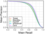
Refer to caption
Refer to caption
Refer to caption
Figure 6: Mean PR curves of different methods on validation sets of SOP (left), iNaturalist (middle), and VehicleID (right).
Refer to caption
Refer to caption
Refer to caption
Figure 7: Convergence results of different methods on validation sets of SOP (left), iNaturalist (middle), and VehicleID (right).