Penetrative convection in nocturnal atmospheric boundary layer and radiation fog

Abstract

After the sunset, under calm and clear sky conditions, aerosol laden surface air-layer, cools radiatively Mukund et al. (2014); Singh et al. (2013) to the upper atmosphere. Predominant effect of the radiative cooling on the vertical temperature profile extends to several hundred meters from the surface. This results in the development of a stable, nocturnal inversion layer. However, ground surface, owing to its higher thermal inertia, lags in the cooling process. Due to this about a meter thick air layer just above the ground can be $(2-6)^{\circ}$C cooler than the ground Ramdas and Atmanathan (1932); Blay-Carreras et al. (2015). Thus, at the surface an unstable convective layer is present, which is capped by a stable inversion layer that extends up to several hundred meters. This configuration involving a convective mixed layer topped by a stably stratified inversion layer is a classic case of penetrative convection Townsend (1964); Adrian (1975). Micro-meteorological phenomenon at the surface, such as occurrence of fog, is determined by temperature profile, heat and moisture transport from the ground. Here, we present a computational study of the model penetrative convection, formed due to radiative cooling, in the nocturnal atmospheric boundary layer.

I Introduction

Penetrative convection, as defined by one of the earlier studies Veronis (1963), involves a convective mixed layer topped by a stably stratified non-turbulent layer. Associated dynamics of penetrative motion of the fluid from the mixed layer into stable layer across the interface, results in entrainment and growth of the mixed layer. This phenomena finds relevance in a wide variety of geophysical and astrophysical problems. The growth of atmospheric daytime boundary layer Driedonks (1982), motions in the outer stable regions of the sun Leighton (1963), the deepening of upper-ocean mixed layer, dynamics of cumulus clouds Simpson et al. (1965), turbulent convection in water over an ice surface Townsend (1964); Adrian (1975) and development of radiation-fog inversion layer are some of the examples.

In all such systems, the two major areas of interest are: $1)$ the convectively driven ‘mixed layer’ and $2)$ dynamics and fluxes through interfacial region sandwiched between turbulent mixed layer and the non-turbulent stably stratified region, often referred to as the ‘entrainment zone’Deardorff, Willis, and Stockton (1980). In order to better understand the formation and subsequent deepening of the convectively driven mixed layer, experimental studies Willis and Deardorff (1974); Kumar (1989) on the structure of turbulence have successfully established the integral length scale and the horizontal velocity scale in the bulk. The length scale is nothing but the depth of the mixed layer (h) and the convection velocity ($U^{*}$) is defined asDeardorff, Willis, and Stockton (1980),

$$U^{*}=\left[\frac{g\beta Q_{b}h}{\rho C_{p}}\right]^{1/3},$$ (1)

where, $g$ is the gravitational constant, $\beta$ is the coefficient of thermal expansion, $\rho$ is the reference density, $C_{p}$ is the specific heat for fluid at constant pressure and $Q_{b}$ is the bottom heat flux. Experimental studies indicate that the thickness of the entrainment zone ($Z_{p}$) could typically reach upto 25 percent of that of the mixed layer Deardorff, Willis, and Stockton (1980). These studies Sreenivas, Arakeri, and Srinivasan (1995); Deardorff, Willis, and Lilly (1969); Deardorff, Willis, and Stockton (1980) emphasize on the importance of entrainment zone physics in understanding phenomena related to the growth/depletion of the mixed layer. The normalized entrainment rate $(U_{e}/U^{*})$, has been shown to be a function of the Richardson number $(Ri)$, with a pre-factor $c$ and an exponent of $n$,

$$\frac{U_{e}}{U^{*}}=c\>\left(Ri^{-n}\right),$$ (2)

where, Richardson number is a widely used non-dimensional parameter that is used to predict the occurrence of fluid turbulence. The definition of $Ri$ in the context of this study is,

$$Ri=\frac{g\left(\Delta\rho\right)h}{\rho(U^{*})^{2}}$$ (3)

$\Delta\rho$ is the density jump across the interface.

Most of the laboratory experiments on penetrative convection Deardorff, Willis, and Lilly (1969); Kumar (1989); Fernando and Little (1990); Sreenivas, Arakeri, and Srinivasan (1995), conducted to establish the aforementioned equations, consist of a stably stratified layer of water and the convection in the system is driven by higher temperature/heat flux at the lower boundary. These configurations allow for a robust and simple experimental controlled environment, but tend to leave out a certain class of penetrative convection problems which find application in atmospheric boundary layers.

The focus of this paper is to study penetrative convection in a class of problems where the system is not driven by a heated boundary, but, by a spatially varying volumetric source/sink term. An aerosol laden atmosphere is a relevant example of such a system, where radiative cooling caused by aerosols, results in some interesting atmospheric phenomena. We specifically focus on the peculiar nature of the nocturnal boundary layer that dates back to Ramdas and co-workers in the 1930’s Ramdas and Atmanathan (1932), where a Lifted Minimum Temperature(LTM) profile was first observed. The origin of which has been demonstrated to be related to radiative flux divergence arising due to the presence of aerosols in the nocturnal atmospheric boundary layer Mukund et al. (2014); Singh et al. (2013). The Ramdas paradox is the occurrence of a counter intuitive temperature minimum, a few tens of centimeters above the ground, on calm and clear nights. After nightfall, under calm and clear sky conditions, atmospheric surface layer close to the ground is shown to cool by aerosol radiation, whereas, the ground lags behind due to its higher thermal inertia Singh et al. (2013); Blay-Carreras et al. (2015). This results in the formation of a convectively driven mixed layer capped above by a stable inversion layer. Under certain environmental conditions, the radiative cooling in the mixed layer causes the air to reach saturation and eventually leads to fog formation. This radiation fog formed near the surface of the ground, thickens, as the air continues to cool and the deepens (overnight), as the stable layer above the fog gets entrained.

In a recent experimental study by Mukund et al.Mukund et al. (2014), major emphasis has been laid on the role of radiative cooling by aerosols in the formulation of the nocturnal boundary layer. It has been established that the inclusion of the radiative flux term in the model, is crucial to obtaining the correct temperature profiles Singh et al. (2013), as seen in Fig.1. Fig.1 depicts the importance of knowing local temperature and dew-point temperature for predicting the onset of fog. It also depicts how fog (liquid aerosol particles) could modify vertical temperature profile through modifying radiation cooling. Experiments carried out by Hutchison and Richards Hutchison and Richards (1999) lay emphasis on the same by studying the effect of radiation on the onset of convection, using carbon dioxide as the participating medium. Recent studies on the Martian atmosphere have also reported the presence of aerosols to be a major cause for fog formation Möhlmann et al. (2009).

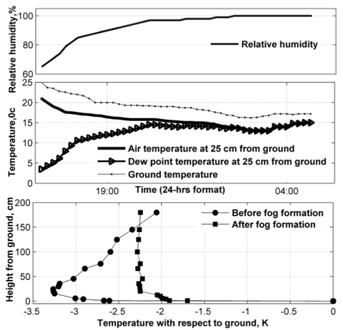
Figure 1: Relative humidity, air temperature, and dew-point temperature at a height of 25 cm above the ground, and ground temperature as a function of time during the night. The vertical temperature profiles above the ground before and after the formation of fog.

In this work, we use the established theoretical understanding of nocturnal boundary layer and radiation fog, to setup a two dimensional simulation domain of $1$m vertical height, with the intent of capturing the LTM, mixed layer and entrainment zone dynamics and subsequently, quantitatively analyze the relationship between the entrainment rate and Richardson number. Dynamics in this layer is typical and has an impact on the occurrence and deepening of the fog layer developed due to radiative cooling Mukund et al. (2014). The correct aerosol number density is important for correctly estimating the radiative flux term. Hence, field and laboratory experiments (see details Singh (2013)) were also carried out in order to estimate the nocturnal aerosol density at relevant heights close to earth’s surface.

Section II of this paper describes the governing equations for the system and also sheds light on field and laboratory experiments carried out to correctly determine the aerosol density, a few decimeters above the surface of the earth. Section III describes the computational setup for running the simulations, highlighting the initial and boundary conditions used in order to closely replicate nocturnal atmospheric conditions. In reality, atmospheric conditions such as aerosol density are seldom consistent and hence, we run the simulation for test cases that span three orders of magnitude in particle number density. We present the mean temperature, density and heat flux profiles in Section IV.1, followed an analysis of the mixed layer and the entrainment zone in Section IV.2.

II Governing equations

The governing equations for the system are conservation of mass, momentum and energy. The system is two dimensional for all purposes in the scope of this paper, with ‘$u$’ being the velocity component in horizontal ($x$) direction and ‘$v$’ being the velocity component in the vertical ($y$) direction. The density, temperature and dynamic viscosity of air is given by $\rho$, $T$ and $\mu$.

$$\frac{d\rho}{dt}+\frac{\partial(\rho u)}{\partial x}+\frac{\partial(\rho v)}{\partial y} =0,$$ (4)

$$\rho\left(\frac{du}{dt}+u\frac{\partial u}{\partial x}+v\frac{\partial u}{\partial y}\right) =\mu\left(\frac{\partial^{2}}{\partial x^{2}}+\frac{\partial^{2}}{\partial y^{2}}\right)u,$$ (5)

$$\rho\left(\frac{dv}{dt}+u\frac{\partial v}{\partial x}+v\frac{\partial v}{\partial y}\right) =\mu\left(\frac{\partial^{2}}{\partial x^{2}}+\frac{\partial^{2}}{\partial y^{2}}\right)v-\rho g,$$ (6)

$$\rho C_{p}\left(\frac{\partial T}{\partial t}+u\frac{\partial T}{\partial x}+v\frac{\partial T}{\partial y}\right) =k\left(\frac{\partial^{2}}{\partial x^{2}}+\frac{\partial^{2}}{\partial y^{2}}\right)T+q^{\prime\prime\prime}.$$ (7)

where, the $g$ is the gravitational constant, $C_{p}$ is the specific heat at constant pressure, $k$ is the thermal conductivity and $q^{\prime\prime\prime}$ is the radiative flux divergence term. The total radiative flux divergence $(q^{\prime\prime\prime})$ is modelled by multiplying the local aerosol number density ($N$) with the net radiative forcing from a single aerosol particle ($Q_{R}$, refer Eq.10),

$$q^{\prime\prime\prime}=N\times Q_{R}.$$ (8)

The non-uniform vertical distribution of aerosols, as indicated in Fig.2, is the primary reason for the observed hyper-cooling being close to the ground. Such a steep variation in number density is common for particulate matter suspended in a fluid Soulsby (1997); Nielsen and Teakle (2004) and is often modelled using a Rouse-profileDevara and Raj (1993); Raj et al. (1997).

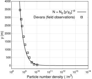
Figure 2: Vertical variation in the number density in a stable, nocturnal boundary layer reported by DevaraDevara and Raj (1993); Raj et al. (1997) along with a Rouse profile fit to the data, where $N_{0}=10840$ x$10^{6}$, $y_{0}=50$ and $p=0.74$

It is worth noting, that in field experiments, the typical height for measurements using lidar, starts from $50$m and extends up to $4$km. In the context of studies revolving around NBL and LTM, the height at which relevant dynamics takes place, we need information within few meters close to ground. Hence, aerosol number densities as a function of height, much closer to the ground, were estimated in a laboratory test sectionSingh (2013).The minimum height from bottom boundary where images are taken is $8$mm, as shown in Fig.3.

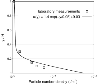
Figure 3: Vertical number density, in the laboratory test section plotted with respect to normalized length scale (y/H, with H=$10$ cm) and $\alpha(y)$ is the non-dimensional absorption coefficient in the test section Singh (2013)

The particle number density as seen in Fig.3, is given by,

$$N=\frac{1}{A}\left[1.4\exp\left(-\frac{y}{0.05}\right)+0.03\right],$$ (9)

and the radiatve flux balance on a single aerosol particle is,

$$Q_{R}=-\frac{\sigma A}{2}\epsilon_{p}\left(\epsilon_{g}T_{g}^{4}+T_{sky}^{4}(2-\epsilon_{g})-2T_{p}^{4}\right),$$ (10)

where, $\sigma$ denotes the Stefan Boltzmann constant and $A$ is the radiative area of spherical aerosol particle. We consider a simplistic case of uniform diameter aerosol particles with a diameter $d=1\mu$m, so the surface area of the sphere is simply $A=\pi d^{2}$(note here that, it is the product of number density N and surface area, that will become important). In Eq.10, $T_{p}$ denotes the temperture of the aerosol particle at a given location, $T_{g}$ is the ground temperature, $T_{sky}$ is the sky temperature, $\epsilon_{g}$ is the ground emissivity and $\epsilon_{p}$ is an area-averaged aerosol emissivity. Corresponding values for temperatures and emmisivities are taken from laboratory experiments Mukund et al. (2014), with $T_{g}=298K$, $T_{sky}=273K$ and $\epsilon_{g}=\epsilon_{p}=0.9$.

The dynamics of aerosol particles is governed by a simple advection-diffusion equation (see Eq. (12).) where the non-dimensional concentration is given by $C$, such that,

$$C=\frac{N-N_{t}}{N_{b}-N_{t}}$$ (11)

where $N_{t}$ and $N_{b}$ are the number density of particles at the top and bottom of the computational domain evaluated using Eq.9. The advection-diffusion for the aerosol is given by,

$$\frac{dC}{dt}+\left(u\frac{d}{dx}+v\frac{d}{dy}\right)C=\delta\left(\frac{\partial^{2}}{\partial x^{2}}+\frac{\partial^{2}}{\partial y^{2}}\right)C$$ (12)

where, $\delta$ is the diffusivity.

III Computational setup

The computational setup is a 2D rectangular domain, $1\text{m}$ in height and $0.75\text{m}$ in width as shown in Fig. 4. The height of the domain is large enough to incorporate the lifted minimum temperature and the mixed layer turbulent dynamics, which is observed a few decimeters above the surface of the ground. The side walls of the domain are kept periodic for mass, momentum and energy in an attempt to model a relatively large section of horizontal ground. Fog can usually span horizontal length scales of few hundred meters and hence, a periodic boundary for the side walls is appropriate for all practical purposes in scope of the problem. The bottom boundary in non-penetrable, non-slip and fixed at a temperature $T_{g}$. For the simulations presented in this paper, we have taken it to be $T_{g}=295.15$K. The top boundary is intended to mimic the night sky at $1\text{m}$ height and an open boundary condition is applied along with a constant heat flux, $q_{t}(=0.1W/m^{2})$. Unlike experiments, where a Dirichlet boundary condition is applied on the top boundary, numerical simulations of this kind facilitate us to use a more realistic radiative flux boundary condition, mimicking radiative cooling and the lapse rate typically observed at $1$m height in the field experiments Mukund et al. (2014). The simulation is initialised with a zero velocity field across the domain and a linear initial temperature profile given by, $T_{0}=\Delta T\>y+T_{g}$, where, $\Delta T=2K$.

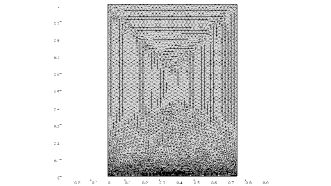
Figure 4: Triangular grid used for computation

Arguably, the most important step in achieving the LTM profile is modelling the radiative cooling term in the energy equation. As show in Eq.8, aerosols are the source of the radiative cooling and flux term is calculated as a product of the number of aerosol particles and the radiative flux from each particle. The initial number density of aerosols as a function of height is taken to be Singh et al. (2013),

$$N_{0}=N_{p}\times\frac{1}{\pi}\left[1.4\exp\left(-\frac{y}{0.05}\right)+0.03\right]\times 10^{12},$$ (13)

as observed in experimentsSingh et al. (2013), where the number density of aerosol particles was measured as close to $8$mm from the ground under clear and calm night conditions. $N_{p}$ is a parameter used to vary the aerosol density and hence the radiative cooling. We run the test problem for a set of three aerosol number densities (see Table1), labelled as Case a), b) and c), with the intent of covering a wide variety of atmospheric conditions that can lead to different orders of magnitude of particle number density. The initial concentration $C_{0}$, for all the cases follows a linear profile with the bottom boundary value of $1$ and a top boundary condition of $0$. The simulation is run for a total time of $10$ minutes with $\Delta t=0.01$ seconds on COMSOL with an extremely fine grid size .

Table 1:

$q_{t}=0.1\>W/m^{2}$	$N_{p}$	$N_{b}\>(/m^{3})$	$N_{t}\>(/m^{3})$
Case a)	$0.1$	$4.55\times 10^{10}$	$9.54\times 10^{8}$
Case b)	$1$	$4.55\times 10^{11}$	$9.54\times 10^{9}$
Case c)	$10$	$4.55\times 10^{12}$	$9.54\times 10^{10}$

IV Results

IV.1 Mean temperature, density and flux profiles

The local temperature and density data from the simulation is first horizontally averaged and then a running average in time (for $30$ seconds) is carried out in order to obtain a temperature and density field, that is solely a function of height and time, devoid of turbulent fluctuations. Fig.5 clearly shows that as the simulation progresses, the stably stratified (linear) initial condition quickly forms an LTM system with the minimum temperature occurring a few tens of centimeters above the lower boundary. This is similar to the LTM profile that is observed at night times under clear and calm conditions. Furthermore, the turbulent mixing in the inversion layer forms an almost isothermal region capped by a stably stratified linear profile on top (typical penetrative convection system). The plots depict the temperature profile for three intermediate times across which the isothermal layer cools and grows progressively. A more detailed analysis of the entrainment of the non turbulent fluid and growth of the mixed layer, is carried out in the next section. Another observation is that the amount of cooling is clearly a function of the number density of the aerosol particles, which in all three cases in Fig 5 is varied using $N_{p}$. Case c) shows the maximum amount of cooling with the mixed layer temperature dropping to $291.6$K after $585$ seconds. Qualitatively, it is easy to notice a faster growth of the mixed layer in Case c), as opposed to Case a), where the mixed layer growth comes to a halt. Similarly the mean density plots are shown in Fig.6 and for all observation purposes mirror the mean temperature plots. In the next section we use the mean density profiles in order to systematically locate the interface in all the simulations.

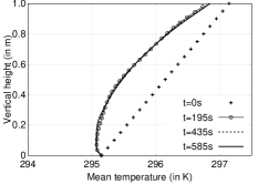
Case a) $\hskip 8.5359ptN_{p}=0.1$

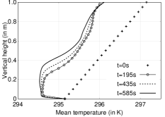
Case b) $\hskip 8.5359ptN_{p}=1$

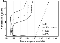
Case c) $\hskip 8.5359ptN_{p}=10$

Figure 5: Mean temperature profiles as a function of vertical height, plotted for four timestamps $t=0,195,435,585$ seconds. The radiative cooling caused by the aerosols leads to the formation of LTM profiles, with growing mixed layers in Case b) and c) and a stagnant mixed layer in Case a).

The divergence of heat flux for conduction, convection and radiation is plotted as a function of height in Fig.7, along with the cooling rate ($dT/dt$ in K/hr), as elements of the balanced heat equation,

$$\frac{\partial T}{\partial t}+\underbrace{\frac{1}{\rho C_{p}}\left(u\frac{\partial}{\partial x}+v\frac{\partial}{\partial y}\right)T}_{\text{convective}}=\underbrace{\frac{k}{\rho C_{p}}\left(\frac{\partial^{2}}{\partial x^{2}}+\frac{\partial^{2}}{\partial y^{2}}\right)T}_{\text{conductive}}+\underbrace{\frac{q^{\prime\prime\prime}}{\rho C_{p}}}_{\text{radiative}}.$$ (14)

At a distance close to the ground, the sharp temperature gradient leads to a substantial conductive flux which is balanced majorly by the convective flux of the upward rising plumes. As we go higher, the conductive flux contribution becomes negligible and the radiative flux terms balances out the convective flux of downward moving plumes. The convective flux contribution also becomes negligible as we reach and cross the interface. As seen in Fig.7, the heat equation is well balanced at all heights and the respective contribution of different heat fluxes follows the expected dynamics of a penetrative convection system.

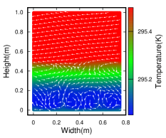
Case a) $\hskip 8.5359ptN_{p}=0.1$

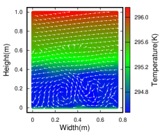
Case b) $\hskip 8.5359ptN_{p}=1$

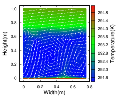
Case c) $\hskip 8.5359ptN_{p}=10$

Figure 6: Mean surface temperature profiles (at $t=585s$) plotted along with average velocity vectors (at $t=585s$). Both temperature and velocity vector, is averaged over the selected time interval $(570-600)s$, for all computational points, and is assigned as the temperature and velocity at $t=585s$.

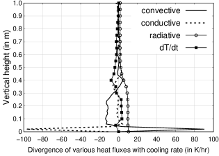
Figure 7: Divergence of heat flux plotted as a function of height for, Case b), $N_{p}=1$. The respective terms of the heat equation (convection, conduction, radiation) are given in Eq.14.

IV.2 Convectively driven mixed layer

Determining the mixed layer height is the first and foremost step for the analysis that follows in subsequent sections. By definition, the mixed layer is a region where turbulent mixing ensures a uniform density. Using this definition and the presence of a stably stratified (linear density) layer on top of the uniform density region, the mixed layer height($h$) is marked as seen in Fig.8 and Fig.9.

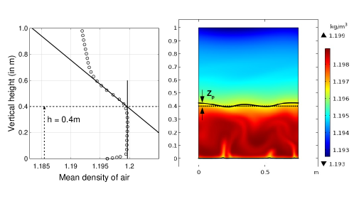
Figure 8: Locating the interface using the density plots for the same instance. a) Horizontally averaged density data. b) Surface plot for density.

Once a mixed layer is formed, the mixed layer height is calculated at every time step and plotted as a function of time in Fig.10. The computational data points seem to very well fit the solid lines that represent a $\propto\sqrt{t}$ dependence, as pointed out in previous studies Kato and Phillips (1969). The rate of change of mixed layer height is termed the entrainment velocity as is simply given by

$$U_{e}=\frac{dh}{dt}$$ (15)

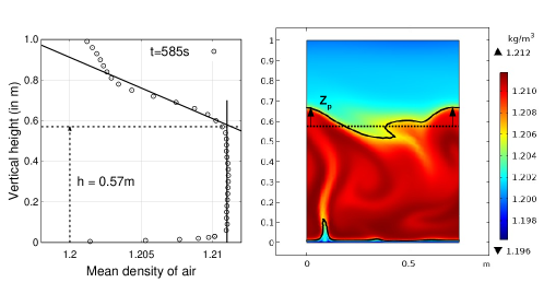
Figure 9: Locating the interface using the density plots for the same instance. a) Horizontally averaged density data. b) Surface plot for density.

Once the mixed layer height is determined,the calculation of convective velocity scale ($U^{*}$) is quite straightforward.

$$U^{*}=\left[\frac{g\beta Q_{b}h}{\rho C_{p}}\right]^{1/3}$$ (16)

where, $g$ is the gravitational constant, $\rho$ is the density and $C_{p}$ is the specific heat for air at constant pressure. $Q_{b}$ is the bottom heat flux and is given by

$$Q_{b}=k\bar{\frac{dT}{dy}}\Big{|}_{y=0}$$ (17)

where $k$ is the thermal conductivity of air.

Figure 10: Growth of the interface height as a function of time

Deardorff’s Deardorff, Willis, and Stockton (1980) turbulent entrainment model for single diffusive systems (alongwith a number of follow up studies) proposes that the entrainment velocity ($U_{e}$) is a function of Richardson number $(Ri)$ and a convective velocity scale $(U^{*})$ given by the relation,

$$U_{e}=C_{1}U^{*}Ri^{-n},$$ (18)

where, $C_{1}$ and $n$ are empirical constants.

Richardson number is a widely used non-dimensional parameter that is used to predict the occurrence of fluid turbulence. It finds practical importance in weather forecasting and in investigating density and turbidity currents in oceans, lakes, and reservoirs. The definition of $Ri$ in the context of this study is,

$$Ri=\frac{g\left(\Delta\rho\right)h}{\rho(U^{*})^{2}}$$ (19)

$\Delta\rho$ is the density jump across the interface. For the calculation of $Ri$, we use the modified turbulent entrainment model Sreenivas, Arakeri, and Srinivasan (1995) to avoid running into a zero $Ri$ problem near the equilibrium, where the model predicts a physically unrealistic entrainment velocity. The modified model divides $\Delta\rho$ into two components $\Delta\rho_{1}$ and $\Delta\rho_{2}$. $\Delta\rho_{1}$, is the density jump across the interface, and typical density profiles shown in Fig. 8 and Fig. 9, suggest that $\Delta\rho_{1}=0$ for all the cases in this study. Jump in density due to the presence of a density gradient is incorporated in the calculation of $\Delta\rho_{2}$. $\Delta\rho_{2}$ is obtained by taking the product of the density gradient $\frac{d\rho}{dy}$ and a relevant length scale. The choice of relevant length scale is crucial to the problem. Choosing the mixed layer height$(h)$ for the length scale, as suggested by some Zangrando and Fernando (1991), leads to an overestimation of the resistance offered by the density gradient to the turbulent entrainment. Previous studies on penetrative convection Deardorff, Willis, and Stockton (1980); Zeman and Tennekes (1977); Sreenivas, Arakeri, and Srinivasan (1995) suggest using the penetration depth $(Z_{p})$ as the relevant length scale. $Z_{p}$ is essentially the distance from the interface into the gradient zone over which the turbulent eddies have an effect.

IV.3 Entrainment Zone

The outermost portion of the mixed layer where stably stratified fluid is entraining but is not yet incorporated into the well-mixed layer is called the ‘entrainment zone ’. The simplest assumption for $Z_{p}$, which has been used by Betts Betts (1976) is

$$Z_{p}=\alpha h$$ (20)

where $\alpha$ is a constant of order $0.3$. This approach doesn’t seem to invoke any physical process to extract $Z_{p}$.

A balance of the kinetic energy per unit volume of the fluid $(KE=\rho(U^{*})^{2}/2)$, in the mixed layer and potential energy gained in lifting a unit volume of fluid $(PE=\Delta\rho Z_{p}g)$ from the interface into the gradient zone to a height of $Z_{p}$ gives,

$$Z_{p}=\sqrt{\frac{\rho\left(U^{*}\right)^{2}}{2g\left(d\rho/dy\right)\big{|}_{y=h}}}$$ (21)

The Richardson number for the problem is thus given by

$$Ri=\frac{g\left(\frac{d\rho}{dy}\Big{|}_{y=h}Z_{p}\right)h}{\rho(U^{*})^{2}}$$ (22)

Once the Richardson number is determined, we use Eq.18 to find the empirical constants $C_{1}$ and $n$ as shown in Fig.13. Now from our simulation, we check the validity of Eq.16 and 21 . In the Fig.11 we present the values of Zp extracted from present simulations and compared that with the expression in Eq.21. Similarly convective velocity scale ($V_{rms}$) observed in the simulations are plotted against that estimated by Eq.16, in Fig.12. Both these estimates compare well over $100$ times increase in aerosol loading simulated here.

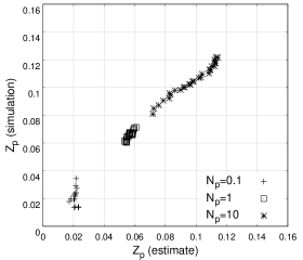
Figure 11: Penetration height ($Z_{p}$) from the simulation (using the protocol in Fig. 8 and Fig. 9) is plotted against the estimated penetration depth as per Eq. 21, for all the three test cases.

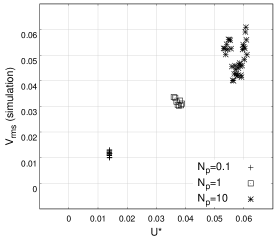
Figure 12: Root mean squared vertical velocity ($V_{rms}$) from the simulation (calculated at the midpoint of the mixed layer) is plotted against the estimated convective velocity scale as per Eq. 16, for all the three test cases.

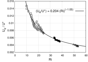
Figure 13: $U_{e}/U^{*}$ plotted as a function of Richardson number. The data is extracted from the three sets of computational experiments and the the fit line gives $C_{1}=0.204$ and $n=1.05$

V Conclusions

In the present work we have simulated LTM type of profiles caused by the radiative cooling of aerosol laden nocturnal surface layer. This cooling develops into a classical penetrative-convection system. We have shown that in this situation, estimation of convective velocity scale ($U^{*}$), entrainment zone thickness ($Z_{p}$) and entrainment velocity (rate of growth of surface mixed layer) can be captured using Deardorff model. However, one must use appropriate scale for $Z_{p}$ as given in Eq.21. Here we show that for $Z_{p}$, one should use height of penetration of buoyant convective parcel into the stratified medium capping the convective mixed layer. This model will be useful in predicting the growth and decay of fog layer in the atmosphere.

Data Availability Statement

The data that support the findings of this study is openly available on gitlab. The link to the same is as follows, https://gitlab.com/shauryajncasr/penetrative-convection-in-nbl

References

- Mukund et al. (2014) V. Mukund, D. Singh, V. Ponnulakshmi, G. Subramanian, and K. Sreenivas, “Field and laboratory experiments on aerosol-induced cooling in the nocturnal boundary layer,” Quarterly Journal of the Royal Meteorological Society 140, 151–169 (2014).
- Singh et al. (2013) D. Singh, V. Ponnulakshami, V. Mukund, G. Subramanian, and K. Sreenivas, “Radiation forcing by the atmospheric aerosols in the nocturnal boundary layer,” in AIP Conference Proceedings, Vol. 1531 (American Institute of Physics, 2013) pp. 596–599.
- Ramdas and Atmanathan (1932) L. Ramdas and S. Atmanathan, “The vertical distribution of air temperature near the ground at night,” Beit. Geophys 37, 116–117 (1932).
- Blay-Carreras et al. (2015) E. Blay-Carreras, E. Pardyjak, D. Pino, S. Hoch, J. Cuxart, D. Martínez, and J. Reuder, “Lifted temperature minimum during the atmospheric evening transition,” Atmospheric Chemistry and Physics 15, 6981–6991 (2015).
- Townsend (1964) A. Townsend, “Natural convection in water over an ice surface,” Quarterly Journal of the Royal Meteorological Society 90, 248–259 (1964).
- Adrian (1975) R. Adrian, “Turbulent convection in water over ice,” Journal of Fluid Mechanics 69, 753–781 (1975).
- Veronis (1963) G. Veronis, “Penetrative convection.” The Astrophysical Journal 137, 641 (1963).
- Driedonks (1982) A. Driedonks, “Models and observations of the growth of the atmospheric boundary layer,” Boundary-Layer Meteorology 23, 283–306 (1982).
- Leighton (1963) R. B. Leighton, “The solar granulation,” Annual review of astronomy and astrophysics 1, 19–40 (1963).
- Simpson et al. (1965) J. Simpson, R. H. Simpson, D. A. Andrews, and M. A. Eaton, “Experimental cumulus dynamics,” Reviews of Geophysics 3, 387–431 (1965).
- Deardorff, Willis, and Stockton (1980) J. Deardorff, G. Willis, and B. Stockton, “Laboratory studies of the entrainment zone of a convectively mixed layer,” Journal of Fluid Mechanics 100, 41–64 (1980).
- Willis and Deardorff (1974) G. Willis and J. Deardorff, “A laboratory model of the unstable planetary boundary layer,” Journal of Atmospheric Sciences 31, 1297–1307 (1974).
- Kumar (1989) R. Kumar, “Laboratory studies of thermal convection in the interface under a stable layer,” International journal of heat and mass transfer 32, 735–749 (1989).
- Sreenivas, Arakeri, and Srinivasan (1995) K. Sreenivas, J. H. Arakeri, and J. Srinivasan, “Modeling the dynamics of the mixed layer in solar ponds,” Solar energy 54, 193–202 (1995).
- Deardorff, Willis, and Lilly (1969) J. W. Deardorff, G. E. Willis, and D. K. Lilly, “Laboratory investigation of non-steady penetrative convection,” Journal of Fluid Mechanics 35, 7–31 (1969).
- Fernando and Little (1990) H. Fernando and L. J. Little, “Molecular-diffusive effects in penetrative convection,” Physics of Fluids A: Fluid Dynamics 2, 1592–1596 (1990).
- Hutchison and Richards (1999) J. Hutchison and R. Richards, “Effect of nongray gas radiation on thermal stability in carbon dioxide,” Journal of thermophysics and heat transfer 13, 25–32 (1999).
- Möhlmann et al. (2009) D. T. Möhlmann, M. Niemand, V. Formisano, H. Savijärvi, and P. Wolkenberg, “Fog phenomena on mars,” Planetary and Space Science 57, 1987–1992 (2009).
- Singh (2013) D. K. Singh, “The impact of aerosols and land surface properties on the lifted temperature minimum in the nocturnal atmospheric boundary layer - field and laboratory experiments,” (2013).
- Soulsby (1997) R. Soulsby, “Dynamics of marine sands,” (1997).
- Nielsen and Teakle (2004) P. Nielsen and I. A. Teakle, “Turbulent diffusion of momentum and suspended particles: A finite-mixing-length theory,” Physics of fluids 16, 2342–2348 (2004).
- Devara and Raj (1993) P. Devara and P. E. Raj, “Lidar measurements of aerosols in the tropical atmosphere,” Advances in atmospheric sciences 10, 365–378 (1993).
- Raj et al. (1997) P. E. Raj, P. Devara, R. Maheskumar, G. Pandithurai, and K. Dani, “Lidar measurements of aerosol column content in an urban nocturnal boundary layer,” Atmospheric research 45, 201–216 (1997).
- Kato and Phillips (1969) H. Kato and O. Phillips, “On the penetration of a turbulent layer into stratified fluid,” Journal of Fluid Mechanics 37, 643–655 (1969).
- Zangrando and Fernando (1991) F. Zangrando and H. Fernando, “A predictive model for the migration of double-diffusive interfaces,” (1991).
- Zeman and Tennekes (1977) O. Zeman and H. Tennekes, “Parameterization of the turbulent energy budget at the top of the daytime atmospheric boundary layer,” Journal of Atmospheric Sciences 34, 111–123 (1977).
- Betts (1976) A. K. Betts, “The thermodynamic transformation of the tropical subcloud layer by precipitation and downdrafts,” Journal of atmospheric sciences 33, 1008–1020 (1976).
- Musman (1968) S. Musman, “Penetrative convection,” Journal of Fluid Mechanics 31, 343–360 (1968).
- Willis and Deardorff (1979) G. Willis and J. Deardorff, “Laboratory observations of turbulent penetrative-convection planforms,” Journal of Geophysical Research: Oceans 84, 295–302 (1979).
- Zdunkowski and Nielsen (1969) W. G. Zdunkowski and B. C. Nielsen, “A preliminary prediction analysis of radiation fog,” pure and applied geophysics 75, 278–299 (1969).
- Ponnulakshmi et al. (2012) V. Ponnulakshmi, V. Mukund, D. , K. Sreenivas, and G. Subramanian, “Hypercooling in the nocturnal boundary layer: Broadband emissivity schemes,” Journal of Atmospheric Sciences 69, 2892–2905 (2012).
- Larson (2000) V. E. Larson, “Stability properties of and scaling laws for a dry radiative-convective atmosphere,” Quarterly Journal of the Royal Meteorological Society 126, 145–171 (2000).
- Larson (2001) V. E. Larson, “The effects of thermal radiation on dry convective instability,” Dynamics of atmospheres and oceans 34, 45–71 (2001).