First results on QCD+QED with C^⋆ boundary conditions

Abstract

Accounting for isospin-breaking corrections is critical for achieving subpercent precision in lattice computations of hadronic observables. A way to include QED and strong-isospin-breaking corrections in lattice QCD calculations is to impose C^⋆ boundary conditions in space. Here, we demonstrate the computation of a selection of meson and baryon masses on two QCD and five QCD+QED gauge ensembles in this setup, which preserves locality, gauge and translational invariance all through the calculation. The generation of the gauge ensembles is performed for two volumes, and three different values of the renormalized fine-structure constant at the U-symmetric point, corresponding to the SU(3)-symmetric QCD in the two ensembles where the electromagnetic coupling is turned off. We also present our tuning strategy and, to the extent possible, a cost analysis of the simulations with C^⋆ boundary conditions.

1 Introduction

At the subpercent level of accuracy the hadronic universe is described by QCD$+$QED. So-called gold-plated hadronic observables, such as meson masses, leptonic and semileptonic decay rates of light pseudoscalar mesons and leading hadronic corrections to the muon $g-2$, are calculated in QCD by means of lattice simulations with a subpercent error (see [1] for a recent review). In order to push the frontier of the precision tests of the hadronic sector of the Standard Model to the subpercent level of accuracy, it is necessary to perform first-principles lattice QCD$+$QED calculations. By now, the necessity of including QED and strong-isospin-breaking corrections in nonperturbative lattice QCD calculations is fully recognized by the lattice community. In practice, this is done by following different approaches and strategies, whose review is beyond the scope of this paper. In our long-term research program, aiming at a precise calculation of the aforementioned gold-plated quantities, we use an approach fully consistent with the basic principles of quantum field theory. QCD$+$QED is defined in finite volume by imposing C^⋆ boundary conditions along the spatial directions, which allows to preserve locality, gauge invariance and translational invariance at all stages of the calculation [7]. We also choose to simulate QCD+QED nonperturbatively, even though our setup can be consistently used also with a perturbative expansion in the electromagnetic coupling constant à la RM123 [8].

In this paper we present a status update of our project. The main results are the masses of the $K^{\pm}$, $K^{0}$, $\pi^{\pm}$, $D^{\pm}$, $D^{0}$ and $D_{s}^{\pm}$ mesons, the $\Omega^{-}$ baryon and the octet baryons, calculated on seven gauge ensembles. The simulations were performed using the openQ*D code [9] at fixed value of the bare strong coupling, three different values of the renormalized fine-structure constant ($\alpha_{R}\simeq 0,1/137,0.04$), two different volumes ($L\simeq 1.6\text{ fm},2.4\text{ fm}$), and heavier-than-physical light-quark masses corresponding to the $U$-spin symmetric point ($m_{s}=m_{d}$).

In full QCD+QED simulations one expects that, except for particularly well-behaved observables, the effect of isospin-breaking corrections may be too small to be resolved against the statistical error. Following [10, 11, 12, 13], we simulate at several values of the fine-structure constant $\alpha_{R}$. In the long run, we want to reduce the error on observables by fitting the functional dependence on $\alpha_{R}$. We define a renormalization (or matching) scheme which allows us to compare QCD+QED at different values of the fine-structure constant. In practice our matching procedure requires the tuning of the bare quark masses in such a way that certain hadronic observables get a prescribed value. Our tuning strategy, designed to keep the cost under control, is described in detail in this paper.

One peculiarity of C^⋆ boundary conditions is that the integration of a dynamical quark field yields the pfaffian of a matrix which is trivially related to the Dirac operator. The fermionic pfaffian is real but not necessarily positive. The absolute value of the pfaffian is included in the simulated probability distribution of the gauge configurations, while its sign is included in the observables as a reweighting factor. It is important to stress that this sign problem is mild, in the sense that the probability to find a negative sign goes to zero in the continuum limit. Nevertheless, a fully local approach to QCD$+$QED requires the evaluation of the sign of the fermionic pfaffian, which we have done systematically for all our configurations. The algorithm used to calculate the sign is based on standard methods which follow the flow of eigenvalues of the hermitian Dirac operator with the quark mass. However, it is worth noticing that our variant is significantly less expensive than similar algorithms commonly used in the lattice community (e.g. [14]). A first version of this algorithm was already presented in [15], an even more optimized version is presented in this paper.

We present also a rather detailed investigation of the computational cost for the generation of our QCD$+$QED configurations with C^⋆ boundary conditions. This is an important piece of information for practitioners who want to choose the most efficient method to calculate observables in QCD+QED. However, one should use this piece of information with a grain of salt. For instance, the generation of QCD+QED configurations is more expensive than QCD ones, but a fair comparison e.g. between full simulations and RM123 method should take into account that observables in the latter method (including all disconnected contributions) are generally more expensive. Similarly, simulations with C^⋆ boundary conditions tend to be more expensive than simulations with periodic boundary conditions, but a fair comparison e.g. between QCD+QED with C^⋆ boundary conditions and QCD+QED_L [16] should take into account that the former has generally smaller non-universal finite-volume effects than the latter. A fair comparison between QCD+QED with C^⋆ boundary conditions and QCD and infinite-volume QED should take into account that the latter has much smaller finite-volume effects than the former, but also a more complicated behavior towards the continuum limit. Besides efficiency considerations, from the theoretical point of view it is extremely important to prove that hadron masses can be computed in a theory with long-range interactions in full compliance with the basic principles of quantum field theory, whatever it takes in terms of computational cost.

The paper is organized as follows. The hadronic renormalization scheme used in this study is presented in section 2, together with the target values of the parameters in the continuum theory. Section 3 provides an overview of numerical setup and results, and is organized in various subsections. The used lattice action, the generated gauge ensembles with corresponding parameters and diagnostic observables are presented in subsections 3.1 and 3.2; meson and baryon masses and mass-differences, calculated on the original and mass-reweighted ensembles, are presented in subsection 3.3; finite-volume effects are discussed in subsection 3.4; a cost analysis for the generation of our ensembles is presented in subsection 3.5. Technical details, which are not essential to the presentation of the general results but are important to guarantee reproducibility, are postponed to section 4 and its subsections. The definition of the used gradient-flow observables is provided in subsection 4.1; the definition of the interpolating operators for mesons and baryons, the strategy used to extract effective masses and identify mass plateaux are discussed in subsections 4.2 and 4.3; a detailed presentation of our tuning strategy is given in subsection 4.4; the methods used for the statistical analysis and in particular for the calculation of the autocorrelation times are outlined in subsection 4.5; the algorithm used to calculate the sign of the pfaffian is discussed in subsection 4.6; the algorithmic parameters are presented in subsection 4.7.

2 Parametrization of four-flavour QCD+QED

Continuum four-flavour QCD+QED is a class of theories uniquely defined by six parameters. The particular choice of these parameters is largely arbitrary, and different choices are often referred to as different renormalization schemes or simply as different schemes. For instance, a renormalization scheme which makes sense in perturbation theory is defined by the $\Lambda_{\text{QCD}}$ in the $\overline{\text{MS}}$ scheme, the renormalized fine-structure constant at zero energy (which is scheme independent) and the four renormalization-group-invariant quark masses. Here we use a nonperturbative scheme defined by the standard gradient-flow scale $(8t_{0})^{1/2}$, the gradient-flow fine-structure constant $\alpha_{R}$ at energy $t_{0}$, and the following dimensionless observables

$$\phi_{0}=8t_{0}(M^{2}_{K^{\pm}}-M^{2}_{\pi^{\pm}})\ ,$$

$$\phi_{1}=8t_{0}(M^{2}_{\pi^{\pm}}+M^{2}_{K^{\pm}}+M^{2}_{K^{0}})\ ,$$

$$\phi_{2}=8t_{0}(M^{2}_{K^{0}}-M^{2}_{K^{\pm}})\alpha_{R}^{-1}\ ,$$

$$\phi_{3}=\sqrt{8t_{0}}(M_{D_{s}^{\pm}}+M_{D^{0}}+M_{D^{\pm}})\ .$$ (2.1)

In the above formulae $M_{X}$ is the mass of the meson $X$. Details on the definition of these observables will be given in the subsequent sections. The convenience of this scheme relies on the fact that all involved observables can be calculated with very good precision and accuracy on the lattice. However, this scheme cannot be used directly to find the physical point, i.e. the point in parameter space which describes the real hadronic universe at the level of subpercent precision, since the scale $t_{0}$ can not be obtained from experimental data. Eventually, the matching to the real hadronic universe needs to be done by going to a hadronic scheme, e.g. by replacing $t_{0}$ with the mass of the $\Omega^{-}$ baryon.

Even though at this stage we are not able to locate the physical point at the subpercent precision level, we can get close to it by using the value of $t_{0}$ calculated by various collaborations via QCD simulations. For instance, using the central value of the CLS determination [19] of $(8t_{0})^{1/2}$, the meson masses and the fine-structure constant from the PDG [20], we obtain for the physical point:

$$(8t_{0}^{\text{phys}})^{1/2}\simeq 0.415\text{ fm}\ ,\quad\alpha_{R}^{\text{phys}}\simeq 1/137\simeq 0.007299\ ,$$ (2.2)

$$\phi_{0}^{\text{phys}}\simeq 0.992\ ,\quad\phi_{1}^{\text{phys}}\simeq 2.26\ ,\quad\phi_{2}^{\text{phys}}\simeq 2.36\ ,\quad\phi_{3}^{\text{phys}}\simeq 12.0\ .$$

As a side remark, the $\phi$ observables have been designed to be maximally sensitive to certain combinations of the quark masses. In fact, at the leading order in SU(3) chiral perturbation theory coupled to QED, one easily shows [21, 22] that

$$\phi_{0}=A(m_{s,R}-m_{d,R})\ ,$$ (2.3a)

$$\phi_{1}=2A(m_{u,R}+m_{d,R}+m_{s,R})+2B\alpha_{R}\ ,$$ (2.3b)

$$\phi_{2}=A\alpha_{R}^{-1}(m_{d,R}-m_{u,R})-B\ ,$$ (2.3c)

where $A$ and $B$ are some low-energy constants, and $m_{\star,R}$ are the renormalized quark masses. The observable $\phi_{0}$ is proportional to the strange/down mass difference. The observable $\phi_{1}$ has been already used in other contexts, e.g. [23, 24], and it fixes the average of the light-quark masses as long as $\alpha_{R}$ is constant. The $\phi_{2}$ observable fixes the ratio between strong and electromagnetic isospin-breaking effects. Finally, the observable $\phi_{3}$ is used essentially to fix the charm quark mass, and has been already used e.g. in [25].

In this paper we present simulations far away from the physical point. There are two main reasons to consider unphysical values of the parameters.

1. We expect that at the physical value of $\alpha_{R}$ we will not be able to have enough statistical precision (except for a handful of observables) to resolve isospin-breaking effects. Following [10, 11, 12, 13], we simulate at several values of the fine-structure constant $\alpha_{R}$, including $\alpha_{R}=0$. Isospin-breaking effects at the physical value of $\alpha_{R}$ can be extracted by interpolation, while keeping the statistical error under control.

2. We simulate up and down quarks that are heavier than the physical ones in order to make simulations less expensive (while the strange quark is lighter than physical). This makes sense especially considering the exploratory character of the presented calculation: our current priority is to investigate the stability of the chosen simulation setup and to develop tuning strategies. The physical value of the quark masses will be approached in future studies.

The simulations presented in this paper are performed close to the unphysical line defined by fixing

$$(8t_{0})^{1/2}=0.415\text{ fm}\ ,\quad\phi_{0}=0\ ,\quad\phi_{1}=2.11\ ,\quad\phi_{2}=2.36\ ,\quad\phi_{3}=12.1\ ,$$ (2.4)

while $\alpha_{R}$ is varied from $0$ to $0.04$. Notice that the condition $\phi_{0}=0$ is equivalent to $M_{K^{\pm}}=M_{\pi^{\pm}}$ and $m_{d}=m_{s}$. When $\phi_{0}=0$, QCD+QED enjoys an enlarged SU(2) flavour symmetry which rotates down and strange quarks into each other, often called U-spin symmetry. For this reason, we will refer to the line in parameter space defined above as the U-symmetric line. Since $\phi_{2}$ is kept constant while $\alpha_{R}$ is varied, in the $\alpha_{R}\to 0$ limit one must have that $M_{K^{0}}=M_{K^{\pm}}$ which also implies that $m_{u}=m_{d}$. Therefore the point $\alpha_{R}=0$ on the U-symmetric line is nothing but SU(3)-symmetric QCD. At this stage, choosing $\phi_{1}$ close to its physical value ensures that the three degenerate light quarks have mass roughly equal to the average of the three physical light-quark masses. The target lines are represented in figure 1, together with the meson masses calculated on our best-tuned ensembles presented in this paper. An overview of our gauge ensembles and of the observables needed for the tuning is given in sections 3.2 and 3.3. Technical details on our tuning strategy are discussed in section 4.4.

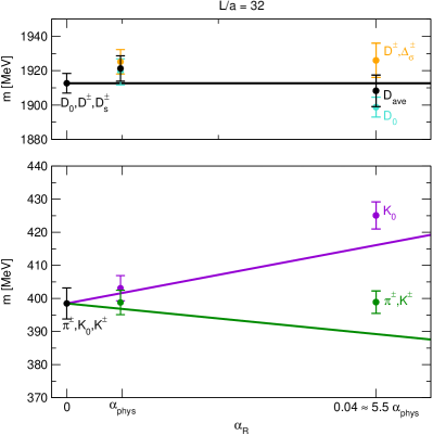
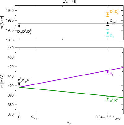
Figure 1: The solid lines are the target values for the $K_{0}$ mass (purple), the $K_{\pm}$ mass (green), the average $D$ mass $M_{D_{\text{ave}}}=\frac{1}{3}(M_{D_{s}^{\pm}}+M_{D_{0}}+M_{D^{\pm}})$ (black) as functions of $\alpha_{R}$, determined by solving the tuning conditions given in eq. (2.4). In the left plots, the data points with error are meson masses calculated on the ensemble A400a00b324 ($\alpha_{R}=0$) and on the reweighted ensembles A380a07b324+RW1 ($\alpha_{R}\simeq 1/137$) and A360a50b324+RW2 ($\alpha_{R}\simeq 0.04$). In the right plots, the data points with error are meson masses calculated on the ensembles B400a00b324 ($\alpha_{R}=0$) and C380a50b324 ($\alpha_{R}\simeq 0.04$). These correspond to our best-tuned ensembles. The comparison between left and right plots indicates how finite-volume effects affect the tuning. For an overview of our gauge ensembles, see section 3.2. The calculation of meson masses and $\phi$ observables is presented in section 3.3. Values in MeV are obtained by using the reference value $(8t_{0})^{1/2}=0.415\text{ fm}$ [19].

3 Overview of numerical results

3.1 Lattice action

All configurations have been generated with the openQ*D code [9]. For a complete description of actions and algorithms we refer the reader to [26], while we provide here only a quick summary.

All our simulations are performed on a $(T/a)\times(L/a)^{3}$ lattice with periodic boundary conditions in time, and C^⋆ boundary conditions in all spatial directions. We employ the Lüscher–Weisz discretization for the SU(3) gauge action, and the Wilson action with an unconventional normalization for the U(1) gauge action

$$S_{\mathrm{g,U(1)}}(z)=\frac{1}{8\pi q_{el}^{2}\alpha}\sum_{x}\sum_{\mu\neq\nu}\left[1-P_{\mu\nu}^{\mathrm{U(1)}}(x)\right]\ ,$$ (3.5)

where $P_{\mu\nu}^{\mathrm{U(1)}}(x)$ is the plaquette in $x$ extending in the directions $\mu$ and $\nu$, constructed with the compact U(1) field $z(x,\mu)$, and $\alpha$ is the bare fine-structure constant. In the compact formulation the electric charge is quantized, and it must be an integer multiple of the parameter $q_{el}$ which can be chosen arbitrarily. In practice, we set $q_{el}=1/6$ which allows us to construct gauge-invariant interpolating operators for charged hadrons as detailed in section 6 of [7]. We simulate at a fixed value $\beta=3.24$ which corresponds roughly to a lattice spacing of $a\simeq 0.054\text{ fm}$, and several values of the bare fine-structure constant $\alpha$.

We simulate four flavours of $O(a)$-improved Wilson fermions. In particular, we consider the non-physical case in which the up and down quarks are heavier than physical, the strange quark is lighter than physical, and the down and strange quarks are degenerate. In the case of QCD+QED the improved Wilson–Dirac operator includes two Sheikholeslami–Wohlert (SW) terms: the first one depends on the SU(3) field tensor with coefficient $c_{\mathrm{sw}}^{\mathrm{SU(3)}}$, and the second one depends on the U(1) field tensor with coefficient $c_{\mathrm{sw}}^{\mathrm{U(1)}}$. For our QCD ensembles we use the improvement coefficient $c_{\mathrm{sw}}^{\mathrm{SU(3)}}$, non-perturbatively determined in [27]. For our QCD+QED ensembles we use the same value of $c_{\mathrm{sw}}^{\mathrm{SU(3)}}$ which is correct up to $O(\alpha)$ terms, and $c_{\mathrm{sw}}^{\mathrm{U(1)}}=1$ which corresponds to tree-level improvement.

Like in the case of periodic boundary conditions, individual flavours of Wilson fermions introduce a mild sign problem. After integrating out the fermions, the path-integral weight is real but generally non-positive. However, the probability to find a negative sign vanishes in the continuum limit. In the case of C^⋆ boundary conditions the sign of the path-integral weight is determined by the sign of the fermionic pfaffian, and has been systematically calculated on our gauge ensembles. Details are given in section 4.6.

3.2 Gauge ensembles

We have generated 7 ensembles with three different values of $\alpha$. The ensembles are named with a string that contains a letter in one-to-one correspondence with the lattice size ($\texttt{A}=64\times 32^{3}$, $\texttt{B}=80\times 48^{3}$, $\texttt{C}=96\times 48^{3}$), the approximative mass of the charged pion, the letter a followed by the two digits in $\alpha=0.0\texttt{xx}\dots$ denoted by x, the letter b followed by the value of $100\times\beta$. The action parameters for all ensembles are summarized in table 1, while the number of generated configurations and a number of diagnostic observables are summarized in table 2.

We observe that, among all observables that we have considered, $t_{0}/a^{2}$ has always the largest integrated autocorrelation time. On our $64\times 32^{3}$ lattices this turns out to be about 100 MDU. On the larger lattices the integrated autocorrelation time of $t_{0}/a^{2}$ seems to be smaller; however, it is reasonable to think that we are just underestimating it because of the reduced statistics. We have also monitored the topological charge, and we observe that we do not incur topological freezing despite using periodic boundary conditions in time (see figure 2).

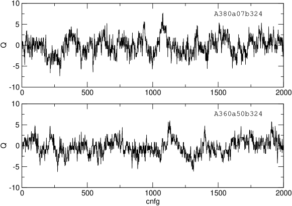
Figure 2: History of the topological charge for two ensembles.

Compact QED displays a first-order phase transition in bare parameter space [28, 29, 30] which separates a strong-coupling confining phase and a weak-coupling Coulomb phase. In the pure gauge theory, the average U(1) plaquette $P^{\mathrm{U(1)}}$ shows a jump across the phase transition: $P^{\mathrm{U(1)}}$ is small in the confining phase and close to 1 in the Coulomb phase. Standard weak- and strong-coupling analysis suggests that the two regimes survive also in presence of fermions. Since we use a compact action for QED and larger than physical values of $\alpha$, a legitimate question is whether we are in the Coulomb phase and far enough from the phase transition. In the conventions of [30], our largest value of $\alpha=0.05$ corresponds to

$$\beta^{\mathrm{U(1)}}=\frac{1}{4\pi q_{el}^{2}\alpha}\simeq 57$$ (3.6)

which is certainly much larger than the critical value $\beta^{\mathrm{U(1)}}_{c}\simeq 1.01$ of the pure gauge theory. The deviation of the average U(1) plaquette from one is $1-P^{\mathrm{U(1)}}=4.19405(21)\times 10^{-3}$ on the ensemble A360a50b324, which is a clear indication that our ensembles are always deep in the weak electromagnetic coupling phase.

ensemble	lattice	$\beta$	$\alpha$	$\kappa_{u}$	$\kappa_{d}=\kappa_{s}$	$\kappa_{c}$
A400a00b324	$64\times 32^{3}$	3.24	0	0.13440733	0.13440733	0.12784
B400a00b324	$80\times 48^{3}$	3.24	0	0.13440733	0.13440733	0.12784
A450a07b324	$64\times 32^{3}$	3.24	0.007299	0.13454999	0.13441323	0.12798662
A380a07b324	$64\times 32^{3}$	3.24	0.007299	0.13459164	0.13444333	0.12806355
A500a50b324	$64\times 32^{3}$	3.24	0.05	0.135479	0.134524	0.12965
A360a50b324	$64\times 32^{3}$	3.24	0.05	0.135560	0.134617	0.129583
C380a50b324	$96\times 48^{3}$	3.24	0.05	0.1355368	0.134596	0.12959326

Table 1: Action parameters. All ensembles have C^⋆ boundary conditions in space and periodic boundary conditions in time. The improvement coefficients are $c_{\mathrm{sw}}^{\mathrm{SU(3)}}=2.18859$ and $c_{\mathrm{sw}}^{\mathrm{U(1)}}=1$.

ensemble	n. cnfg	acc. rate	$\langle e^{-\Delta H}\rangle$	$\tau_{\mathrm{int}}(t_{0})$	$\tau_{\mathrm{int}}(Q^{2})$	$\tau_{\mathrm{int}}(\alpha_{R})$
A400a00b324	2000	95%	0.9979(55)	51(18)	6.4(2.3)	—
B400a00b324	1082	98%	0.9950(25)	31(10)	8.0(2.8)	—
A450a07b324	1000	94%	0.9978(46)	44(19)	6.5(3.0)	2.3(1.6)
A380a07b324	2000	92%	1.0017(46)	46(15)	10.3(3.5)	2.7(1.5)
A500a50b324	1993	97%	0.9961(21)	21.4(5.5)	11.6(2.6)	1.40(55)
A360a50b324	2001	95%	0.9956(45)	47(16)	8.5(2.6)	1.1(1.0)
C380a50b324	600	98%	1.004(12)	12.5(3.9)	10.6(4.1)	3.0(1.2)

Table 2: For each ensemble: the number of configurations which corresponds to the number of MD trajectories, the acceptance rate, the diagnostic observable $\langle e^{-\Delta H}\rangle=1$, the integrated autocorrelation times (in units of MD trajectories) for the scale $t_{0}/a^{2}$, the squared topological charge $Q^{2}$, and the renormalized fine-structure constant $\alpha_{R}$. One MD trajectory is equal to $\tau=2$ MD units.

3.3 Tuning and hadron masses

Once the theory is discretized on the lattice, it depends on six dimensionless bare parameters: the inverse bare strong coupling $\beta$, the bare fine-structure constant $\alpha$ and the hopping parameters $\kappa_{f}$. In our simulation strategy these six parameters are treated in different ways: we choose the values of $\beta$ and $\alpha$, while we tune the values of $\kappa_{f=u,d,s,c}$. Changing $\beta$ changes the lattice spacing, and eventually we want to simulate at different values of $\beta$ and then take the continuum limit by extrapolating to $\beta\to\infty$. Pretty much like in QCD, we do care about choosing $\beta$ in a range such that the lattice spacing is as fine as we can afford, but we do not care about tuning the lattice spacing to specific values. If we wanted to match the renormalized fine-structure constant $\alpha_{R}$ to its physical value, we would need to tune the bare fine-structure constant $\alpha$. Instead we only want to scan several values of $\alpha_{R}$, which means that we can choose the value of $\alpha$ in a reasonable range and then simply calculate $\alpha_{R}$. On the other hand, for each chosen value of $\beta$ and $\alpha$, we want to tune the four hopping parameters $\kappa_{f}$ in such a way that the four dimensionless $\phi$ observables match the chosen values in eq. (2.4). In fact, on the U-symmetric line, U-spin symmetry fixes $m_{d}=m_{s}$ and we truly have to tune only three parameters. Finally, values of observables in lattice units are converted into physical units by using the reference value for $t_{0}$ given in eq. (2.4).

The tuning of the hopping parameters has been carried out with a combination of techniques, described in some detail in section 4.4. In particular, we have used mass reweighting to explore the space of hopping parameters in the vicinity of the simulated point. The specific implementation of the mass reweighting procedure used in this work is described in [31], the peculiarity being that we need to reweight the determinant of the rational approximation of a generic power of $D^{\dagger}D$. One can use mass reweighting also to correct for small mistunings, which we have done to some extent. We label all mass reweighting factors used in this work by the code RWi where i is an index. In table 3 we summarize all mass reweighting factors, together with the ensembles on which they are calculated and the target quark hopping parameters.

The calculated values of the lattice spacing $a$ and renormalized fine-structure constant, with and without mass reweightings, are presented in table 4. Some details on the calculation of these observables are given in sections 4.1. We have calculated the masses of the $\pi^{\pm}$, $K_{0}$, $K^{\pm}$, $D_{0}$, $D^{\pm}$, $D_{s}^{\pm}$ mesons, and the mass differences for the charged-neutral $K$ mesons and $D$ mesons: results are presented in table 5 and the methods used are described in section 4.2. It is interesting to notice that, at the tuned points, we are able to distinguish clearly the $K_{0}/K^{\pm}$ mass difference from zero even at the physical value of $\alpha_{R}$, while the signal is somewhat less clear for the $D_{0}/D^{\pm}$ mass difference. The $\phi$ observables, which are used for tuning, are presented in table 6. Notice that, at the tuned points, we were able to determine $\phi_{1}$ with a relative statistical error of about 3%, $\phi_{2}$ with a relative statistical error in the range 5-10%, and $\phi_{3}$ with a relative statistical error of 0.5%. Unsurprisingly, since $\phi_{2}$ is proportional to the isospin-breaking corrections, it is the hardest to get, especially at smaller values of $\alpha_{R}$. The meson masses calculated at the tuned points are plotted in figure 1.

We have also calculated the masses of the octet baryons and the $\Omega^{-}$ baryon in all our small-volume QCD+QED ensembles, together with various baryon mass differences: the results are presented in tables 7 and 8. A description of the methods used in this calculation, together with the plots of a selection of effective masses, can be found in section 4.3. Here we notice that we obtain baryon masses with a statistical error in the range 1-5%, while the statistical error on the baryon mass differences is less uniform. As expected, the statistical error on the baryon masses is generally higher for ensembles with heavier pions. The baryon masses measured on our ensemble A360a50b324+RW2 ($\alpha_{R}\simeq 0.04$) have significantly larger errors than the other ensembles. This can be due to a combination of factors: lighter pions, smaller number of stochastic sources, and perhaps larger effect of the reweighting factor. We plan to investigate this issue in the future. We have not attempted a systematic study of excited state contaminations (which is milder for heavier-than-physical pions) and we do not attempt an estimate of the systematic error due to a misidentification of the plateau region in our effective masses, but we have checked the stability of our results against the inclusion of interpolating operators with different levels of smearing in a generalized eigenvalue problem.

As discussed in [7], C^⋆ boundary conditions partially break flavour symmetries producing some unphysical mixings, which are pure finite-volume effects and vanish exponentially fast in the infinite-volume limit even in QCD+QED. Of the considered baryons, the $\Xi^{-}$ mixes with the proton, the $\Xi^{0}$ mixes with the neutron, and the $\Omega^{-}$ mixes with the $\Sigma^{*+}$. In practice, these mixings are generated by quark-disconnected Wick contractions in the baryon-baryon two-point functions which are allowed because of the boundary conditions. In our calculation we neglect these disconnected contributions, which means that we truly consider partially-quenched baryons made of auxiliary valence quarks for which the mixing is forbidden. For instance our $\Omega^{-}$ is truly an $ss^{\prime}s^{\prime\prime}$ baryon where $s^{\prime}$ and $s^{\prime\prime}$ are valence quarks with the same mass and charge as the strange quark $s$. The two-point functions of these partially-quenched baryons differ from the two-point functions of the unitary baryons by exponentially suppressed finite-volume effects.

reweighting	ensemble	$\kappa_{u}$	$\kappa_{d}=\kappa_{s}$	$\kappa_{c}$
RW1	A380a07b324	0.13457969	0.13443525	0.12806355
RW2	A360a50b324	0.13553680	0.1345960	0.12959326

Table 3: For each mass reweighting factor: the ensemble on which it is calculated and the target values of the hopping parameters.

ensemble(+rw)	$t_{0}/a^{2}$	$a$ [fm]	$\alpha_{R}$	$\pi\sqrt{3}L^{-1}$ [MeV]
A400a00b324	7.402(66)	0.05393(24)	0	—
B400a00b324	7.383(40)	0.05400(14)	0	—
A450a07b324	7.198(84)	0.05469(32)	0.007076(24)	613.5(3.6)
A380a07b324	7.599(79)	0.05323(28)	0.007081(19)	630.4(3.3)
A380a07b324+RW1	7.525(77)	0.05349(27)	0.007080(22)	627.3(3.2)
A500a50b324	7.789(42)	0.05257(14)	0.040772(85)	638.2(1.7)
A360a50b324	8.427(89)	0.05054(27)	0.040633(80)	663.9(3.5)
A360a50b324+RW2	8.285(79)	0.05098(24)	0.04069(26)	658.2(3.2)
C380a50b324	8.400(26)	0.050625(79)	0.04073(11)	441.86(69)

Table 4: For each ensemble (possibly with mass reweighting): reference observable $t_{0}/a^{2}$, lattice spacing $a$ calculated from the measured value of $t_{0}/a^{2}$, the renormalized fine-structure constant $\alpha_{R}$, the tree-level energy gap of the photon $\pi\sqrt{3}L^{-1}$. Values in physical units are obtained by using the reference value $(8t_{0})^{1/2}=0.415\text{ fm}$ [19].

ensemble(+rw)	$M_{\pi^{\pm}}=M_{K^{\pm}}$	$M_{K_{0}}$	$M_{K_{0}}-M_{K^{\pm}}$	$M_{D^{\pm}}=M_{D_{s}^{\pm}}$	$M_{D_{0}}$	$M_{D^{\pm}}-M_{D^{0}}$
	[MeV]	[MeV]	[MeV]	[MeV]	[MeV]	[MeV]
A400a00b324	398.5(4.7)	398.5(4.7)	0	1912.7(5.7)	1912.7(5.7)	0
B400a00b324	401.9(1.4)	401.9(1.4)	0	1908.5(4.5)	1908.5(4.5)	0
A450a07b324	451.2(4.3)	451.6(4.7)	0.8(1.1)	1919.8(7.3)	1916.0(8.0)	3.6(1.2)
A380a07b324	383.6(4.4)	390.7(3.7)	7.01(26)	1926.4(7.8)	1921.1(7.6)	5.03(46)
A380a07b324+RW1	398.8(3.7)	403.1(3.8)	4.26(31)	1925.2(7.1)	1919.3(7.6)	5.8(1.1)
A500a50b324	495.0(2.8)	519.1(2.5)	24.0(1.0)	1901.1(4.1)	1870.1(4.4)	31.6(1.6)
A360a50b324	358.6(3.7)	388.8(3.5)	29.5(2.4)	1937.8(6.8)	1912.0(7.7)	26.0(2.8)
A360a50b324+RW2	398.9(3.4)	425.1(4.1)	26.1(1.3)	1926(10)	1898.8(5.8)	26.9(2.2)
C380a50b324	386.5(2.4)	414.5(2.0)	26.89(49)	1932.0(3.9)	1894.3(6.9)	34.5(5.6)

Table 5: For each ensemble (possibly with mass reweighting): meson masses, and charged-neutral meson mass differences. Values in MeV are obtained by using the reference value $(8t_{0})^{1/2}=0.415\text{ fm}$ [19]. Notice that some mesons are degenerate because in our simulations $m_{d}=m_{s}$.

ensemble(+rw)	$\phi_{1}$	$\phi_{2}$	$\phi_{3}$
A400a00b324	2.107(50)	—	12.068(36)
B400a00b324	2.143(15)	—	12.042(28)
A450a07b324	2.703(53)	0.44(60)	12.097(51)
A380a07b324	1.977(37)	3.39(14)	12.132(48)
A380a07b324+RW1	2.126(39)	2.13(17)	12.122(47)
A500a50b324	3.357(37)	2.60(11)	11.864(28)
A360a50b324	1.806(35)	2.41(19)	12.114(41)
A360a50b324+RW2	2.208(38)	2.348(97)	12.040(58)
C380a50b324	2.088(22)	2.350(44)	12.020(29)
target	2.11	2.36	12.1

Table 6: $\phi$ parameters for each ensemble (possibly with mass reweighting), together with the target value used to define the lines of constant physics.

ensemble(+rw)	$M_{p}=M_{\Sigma^{+}}$	$M_{n}=M_{\Xi^{0}}$	$M_{\Xi^{-}}=M_{\Sigma^{-}}$	$M_{\Lambda^{0}}$	$M_{\Omega^{-}}=M_{\Delta^{-}}$
	[MeV]	[MeV]	[MeV]	[MeV]	[MeV]
A450a07b324	1214(14)	1215(15)	1216(16)	1215(15)	1473(35)
A380a07b324	1147(19)	1151(19)	1157(18)	1151(19)	1458(26)
A380a07b324+RW1	1164(15)	1167(13)	1175(14)	1167(13)	1448(20)
A500a50b324	1280(15)	1288(13)	1339(11)	1296(13)	1614(23)
A360a50b324+RW2	1212(20)	1226(22)	1268(32)	1227(24)	1584(59)

Table 7: For each ensemble (possibly with mass reweighting): baryon masses. Values in MeV are obtained by using the reference value $(8t_{0})^{1/2}=0.415\text{ fm}$ [19]. Notice that some baryons are degenerate because in our simulations $m_{d}=m_{s}$.

ensemble(+rw)	$M_{n}-M_{p}$	$M_{\Xi^{0}}-M_{\Xi^{-}}$	$M_{\Sigma^{+}}-M_{\Sigma^{-}}$
	[MeV]	[MeV]	[MeV]
A450a07b324	-0.89(0.38)	-2.44(0.49)	-1.77(0.89)
A380a07b324	1.80(0.52)	-8.37(0.75)	-9.96(0.79)
A380a07b324+RW1	0.90(0.37)	-5.97(0.63)	-6.81(0.68)
A500a50b324	9.2(1.5)	-38.2(2.4)	-46.7(2.7)
A360a50b324+RW2	10.5(6.0)	-30.2(4.7)	-52(11)

Table 8: For each ensemble (possibly with mass reweighting): baryon mass differences. Values in MeV are obtained by using the reference value $(8t_{0})^{1/2}=0.415\text{ fm}$ [19].

3.4 Finite-volume effects

Most of the presented ensembles correspond to a $64\times 32^{3}$ lattice. In order to estimate finite volume effects, we have generated two larger lattices: an $80\times 48^{3}$ lattice for $\alpha=0$ and a $96\times 48^{3}$ for $\alpha=0.05$. This allows us to get an idea of the finite-volume effects in particular on the light meson masses.

In the QCD case, our spatial volumes correspond to $M_{\pi}L\simeq 3.5$ for the A400a00b324 ensemble and $M_{\pi}L\simeq 5.2$ for the B400a00b324 ensemble. It is useful to compare our results with the ones of the ALPHA collaboration [25] obtained with periodic boundary conditions (the action parameters are identical). In figure 3 we show the pion mass for two volumes and different boundary conditions. It is interesting to notice that finite volume corrections tend to increase the mass in the case of periodic boundary conditions, while they tend to decrease the mass in the case of C^⋆ boundary conditions. This behaviour is captured by chiral perturbation theory at leading order (for the periodic case see e.g. [32]):

$$M_{\text{P}}(L)=M+\frac{\xi}{3}\sum_{\mathbf{n}\in\mathbb{Z}^{3}\setminus\{0\}}\frac{2}{L}K_{1}(nML)\ ,$$ (3.7)

$$M_{\text{C}}(L)=M-\frac{\xi}{3}\sum_{\mathbf{n}\in\mathbb{Z}^{3}\setminus\{0\}}\frac{1-3(-1)^{\sum_{k}n_{k}}}{nL}K_{1}(nML)\ ,$$ (3.8)

where $n=|\mathbf{n}|$, $\xi=M^{2}/(4\pi F)^{2}$ with $F$ being the pion decay constant, $K_{1}$ is a modified Bessel function of the second kind, the subscripts P and C denote periodic and C^⋆ boundary conditions, respectively. In figure 3 we plot also the result of the simultaneous fits with the two above functions in the parameters $M$ and $\xi$. On the large volumes, finite volume effects on the pion mass are surely not larger than 1%. While the statistical errors on the pion masses on the smaller volumes are fairly large and a definite interpretation would require higher statistics, figure 3 suggests that finite volume effects are sizable in this case.

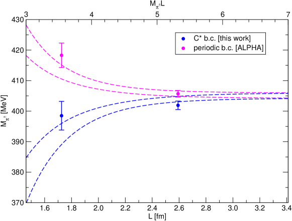
Figure 3: Pion masses for our A400a00b324 and B400a00b324 ensembles with C^⋆ boundary conditions, and for the A1 and A2 from [25] with periodic boundary conditions. In both cases physical units have been introduced by setting $(8t_{0})^{1/2}=0.415\text{ fm}$ [19]. The curves are the results of the simultaneous fit to the LO $\chi$PT formulae with uncertainty bands.

When QCD is coupled to QED the pion mass gets power corrections which vanish like inverse powers of the volume. In the case of C^⋆ boundary conditions these finite-volume effects have been derived in [7]:

$$M_{\text{C}}(L)=M-\alpha\left\{\frac{q^{2}\zeta(1)}{2L}+\frac{q^{2}\zeta(2)}{\pi ML^{2}}+\sum_{\ell=0}^{\infty}\frac{(-1)^{\ell}\zeta(2\ell+2)}{4\pi ML^{4+2\ell}}T_{\ell}\right\}+O(\alpha^{2})\ ,$$ (3.9)

where $q$ is the charge of the pion, the generalized zeta function $\zeta(p)$ is defined by

$$\zeta(p)=\sum_{\mathbf{n}\in\mathbb{Z}^{3}\setminus\{0\}}\frac{(-1)^{\sum_{k}n_{k}}}{|\mathbf{n}|^{p}}\ ,$$ (3.10)

and the coefficients $T_{\ell}$ are related to the coefficients of the Taylor expansion with respect to the on-shell photon energy of the forward Compton scattering amplitude of the pion (for more details see [7]). The first two terms of the $1/L$-expansion are structure independent and they have been already subtracted in all hadron masses presented in the tables of this paper, accordingly to the procedure detailed in section 4.2. The only exception is table 9, in which we present the masses of charged mesons for a couple of ensembles without the subtraction of the structure-independent finite-volume effects, and with the subtraction of only the $1/L$ term. For the charged pion on our C380a50b324 ensemble ($L/a=48$ and $\alpha=0.05$), the structure-independent contributions to the finite-volume effects turn out to be about 0.9% and most of the effect comes from the leading $1/L$ term. Hence it is reasonable to assume that QED finite-volume effects are well under control in our largest volume, even though a more detailed study would be desirable.

	$M_{\pi^{\pm}}=M_{K^{\pm}}$ [MeV]			$M_{D^{\pm}}=M_{D^{\pm}_{s}}$ [MeV]
ensemble(+rw)	no-FV	LO-FV	NLO-FV	no-FV	LO-FV	NLO-FV
A360a50b324+RW2	393.4(3.4)	397.7(3.4)	398.9(3.4)	1922(10)	1926(10)	1926(10)
C380a50b324	383.1(2.4)	386.0(2.4)	386.5(2.4)	1929.0(3.9)	1931.9(3.9)	1932.0(3.9)

Table 9: For the two ensemble with $\alpha_{R}\simeq 0.04$ and tuned values of the quark masses: $\pi^{\pm}$ and $D_{\pi^{\pm}}$ masses calculated with no subtraction of the structure-independent finite-volume corrections (no-FV), with the subtraction of only the $1/L$ finite-volume correction (LO-FV), with the subtraction of the $1/L$ and $1/L^{2}$ finite-volume corrections (NLO-FV). The $1/L^{2}$ finite volume correction produces a 0.3% shift on the $\pi^{\pm}$ mass on the smaller volume, and a 0.1% shift on the $\pi^{\pm}$ mass on the larger volume. Values in MeV are obtained by using the reference value $(8t_{0})^{1/2}=0.415\text{ fm}$ [19].

3.5 Note on simulation cost

Our production runs have been performed on a variety of machines: Lise at HRLN, Marconi at CINECA, Eagle at PSNC and Piz Daint at CSCS. In order to be able to compare the production cost, we have measured the time needed to generate a thermalized configuration on Lise at HLRN for all gauge ensembles. The results are shown in table 10; in particular, we report the specific cost, i.e. the cost in core$\times$seconds per molecular dynamics unit divided by the number of lattice points. Comparing specific costs makes sense particularly if the machine is always used in a regime of reasonably good scaling, which seems to be the case for the presented runs. In table 10 we have also reported the production cost for the QCD ensemble A1 generated by the ALPHA collaboration on Lise and presented in [25]. The production cost is not reported in the paper and has been kindly provided by the authors of [25].

The ensemble A1 can be compared directly with our ensemble A400a00b324. The two QCD ensemble use the same discretization of the action, the same values of $\beta$, bare quark masses and improvement coefficients, but differ for the volume and the boundary conditions. The ensemble A1 uses a $96\times 32^{3}$ lattice with open boundary conditions in time and periodic boundary conditions in space, while our ensemble A400a00b324 uses a $64\times 32^{3}$ lattice with periodic boundary conditions in time and C^⋆ boundary conditions in space. The two ensembles differ also by a number of algorithmic parameters, rendering a precise cost comparison between the two ensembles complicated. In the following, we use a back-of-the-envelope calculation to argue that we understand the most important effects contributing to the cost ratio:

$$\left[\frac{\text{specific cost}(\texttt{A400a00b324})}{\text{specific cost}(\texttt{A1})}\right]_{\text{measured}}\simeq\frac{0.42}{0.35}=1.2\ .$$ (3.11)

1. Because of C^⋆ boundary conditions, the Dirac operator is a matrix that acts on a vector space with dimension $24V$, as opposed to $12V$ in case of periodic boundary conditions. This means that the application of the Dirac operator on a single pseudofermion costs twice as much as the periodic case if the physical volume is the same. C^⋆ boundary conditions contribute with a factor of two to the ratio (3.11).

2. A three-level integrator has been used in both cases: 8 steps of second-order Omelyan in the outermost level, 1 step of fourth-order Omelyan in the intermediate level, 1 step (for A400a00b324) or 2 steps (for A1) of fourth-order Omelyan in the innermost level. The difference in the innermost level is expected not to have a significant impact on the total cost since only the gauge forces are integrated in that level in both cases. Therefore, we estimate that the difference in integrator steps contributes with a factor of roughly one to the ratio (3.11).

3. In the case of the ensemble A1, the HMC with frequency splitting has been used for the up/down doublet and two different rational approximations have been used for the strange and charm. In the case of the ensemble A400a00b324, a single rational approximation has been used for the degenerate up/down/strange triplet, and a separate rational approximation has been used for the charm. In spite of this difference, it turns out that the total number of fermionic forces that need to be calculated is not so different in the two cases. For A400a00b324 and A1, the outermost level integrates six and five pseudofermion forces, respectively, and the intermediate level integrates six and eight pseudofermion forces, respectively. Since the forces of the intermediate level are calculated much more often than the ones on the outer level, we consider only the intermediate level for this back-of-the-envelope calculation. Therefore, we estimate that the difference in pseudofermion forces contributes with a factor of roughly $6/8=0.75$ to the ratio (3.11) (reducing the cost gap between the two ensembles).

4. Smaller residues have been typically used in A1 for the solvers used to calculate pseudofermion forces, reducing the cost gap between A400a00b324 and A1 even further. The impact of this effect has been estimated by looking at how many times the Dirac operator is applied by the various solvers. We estimate that the difference in residues contributes with a factor of roughly $0.84$ to the ratio (3.11) (further reducing the cost gap between the two ensembles).

Multiplying all the above factors together we obtain the following estimate for the cost ratio

$$\left[\frac{\text{specific cost}(\texttt{A400a00b324})}{\text{specific cost}(\texttt{A1})}\right]_{\text{estimated}}\simeq 2\times 1\times 0.75\times 0.84=1.26\ ,$$ (3.12)

which is remarkably close to the measured ratio (3.11).

The comparison between A380a07b324 and A360a50b324 (fairly similar algorithmic parameters where used in these two runs) suggests that the computational cost does not depend significanly on $\alpha$ in the interesting region. The comparison between these two ensembles on the one hand and the ensemble A400a00b324 on the other hand shows a clear cost gap between the QCD+QED and QCD simulations, yielding e.g.

$$\left[\frac{\text{specific cost}(\texttt{A360a50b324})}{\text{specific cost}(\texttt{A400a00b324})}\right]_{\text{measured}}\simeq\frac{1.05}{0.42}=2.5\ .$$ (3.13)

In a certain measure this is due to physics: the QCD ensemble has an SU(3) flavour symmetry which allows us to use a single rational approximation for the three light quarks, while the QCD+QED ensembles have only an SU(2) flavour symmetry forcing us to use a rational approximation for the up quark and a different rational approximation for the down/strange quarks. However we also notice that we need to increase the number of integration steps in our QCD+QED ensembles (from 8 to 12 in the outermost level) in order to keep the acceptance rate to a reasonable level. The source of this effect is unclear, and we plan to investigate in the future whether it is possible to avoid it by optimizing the algorithmic parameters.

The specific cost is essentially the same for the A380a07b324 and A450a07b324 ensembles, modulo fluctuations in performance. In particular we detect no significant dependence on the light quark masses.

The increase in specific cost from the A360a50b324 to the C380a50b324 is completely accounted for by the increase in the number of integration steps in the outermost level (from 12 to 18) needed to compensate the reduction in acceptance rate due to the larger volume. However, a posteriori we have overdone it, and we could have probably used some intermediate value. The increase in specific cost from the A400a00b324 to the B400a00b324 is partly accounted for by the increase in the number of integration steps in the outermost level (from 12 to 16), while the extra cost may be due to a decrease in efficiency due to use of a highly-asymmetric local lattice.

More details on the choice of algorithmic parameters are provided in section 4.7.

ensemble	global volume	n. cores	specific cost
			$\left[\frac{\text{cores}\times\text{secs}}{\text{MDUs}\times\text{points}}\right]$
A1 [25]	$96\times 32^{3}$	6144	0.35
A400a00b324	$64\times 32^{3}$	4096	0.42
B400a00b324	$80\times 48^{3}$	2560	0.62
A450a07b324	$64\times 32^{3}$	4096	1.07
A380a07b324	$64\times 32^{3}$	4096	1.03
A500a50b324	$64\times 32^{3}$	4096	0.88
A360a50b324	$64\times 32^{3}$	4096	1.05
C380a50b324	$96\times 48^{3}$	3072	1.40

Table 10: Cost comparison of all production runs presented in this paper, plus the $N_{f}=3+1$ QCD ensemble A1 produced by the ALPHA collaboration [25]. All wall times have been measured on Lise at HLRN. For each run we report the global lattice volume, the number of cores, and the specific cost i.e. the cost in coresecs per molecular dynamics unit (MDU) divided by the global volume.

4 Technical details

4.1 Flow observables

The gradient flow is used to define the auxiliary observable $t_{0}$ and the renormalized fine-structure constant $\alpha_{R}$. In particular, we use the Wilson-flow discretization [33] for the SU(3) flow equation

$$a^{2}\partial_{t}U_{t}(x,\mu)=-g^{2}\left\{\partial_{x,\mu}S_{\mathrm{w,SU(3)}}(U_{t})\right\}U_{t}(x,\mu)\ ,$$ (4.14)

where $U_{t}$ is the SU(3) gauge field at positive flow time, and $S_{\mathrm{w,SU(3)}}(U)$ is the standard SU(3) Wilson action. For the U(1) flow equation we use the obvious generalization

$$a^{2}\partial_{t}z_{t}(x,\mu)=-4\pi\alpha\left\{\partial_{x,\mu}S_{\mathrm{g,U(1)}}(z_{t})\right\}z_{t}(x,\mu)\ ,$$ (4.15)

where $z_{t}$ is the compact U(1) gauge field at positive flow time, $S_{\mathrm{g,U(1)}}(z)$ is the action given in eq. (3.5). If $\hat{G}_{t,\mu\nu}(x)$ and $\hat{F}_{t,\mu\nu}(x)$ are, respectively, the clover discretizations of the SU(3) and U(1) field tensors at positive flow time, we define the clover action densities as

$$E_{\mathrm{SU(3)}}(t)=\frac{1}{2}\sum_{\mu\nu}\langle\operatorname{tr}\hat{G}_{t,\mu\nu}^{2}\rangle\ ,\qquad E_{\mathrm{U(1)}}(t)=\frac{1}{4q_{el}^{2}}\sum_{\mu\nu}\langle\hat{F}_{t,\mu\nu}^{2}\rangle\ .$$ (4.16)

The auxiliary observable $t_{0}$ is defined as usual by means of the equation

$$t_{0}^{2}E_{\mathrm{SU(3)}}(t_{0})=0.3\ ,$$ (4.17)

while the renormalized fine-structure constant is defined at the scale $t_{0}$ as

$$\alpha_{R}=\mathcal{N}t_{0}^{2}E_{\mathrm{U(1)}}(t_{0})\ .$$ (4.18)

Following [34], the normalizaton $\mathcal{N}$ is chosen in such a way that $\alpha_{R}$ coincides with $\alpha$ at tree level in the lattice perturbative expansion. Its explicit formula is given by

$$\mathcal{N}^{-1}=\frac{2\pi t_{0}^{2}}{TL^{3}}\sum_{p}\frac{\sum_{\mu\nu}\mathring{p}_{\mu}^{2}c_{\nu}^{2}-\sum_{\mu}\mathring{p}_{\mu}^{2}c_{\mu}^{2}}{\sum_{\mu}\hat{p}_{\mu}^{2}}e^{-2t_{0}\sum_{\mu}\hat{p}_{\mu}^{2}}\ ,$$ (4.19)

where the sum runs over all momenta allowed by the boundary conditions

$$p_{0}\in\frac{2\pi a}{T}\left\{0,1,2,\dots,\frac{T}{a}-1\right\}\ ,\qquad p_{k}\in\frac{\pi a}{L}\left\{1,3,5,\dots,\frac{2L}{a}-1\right\}\ ,$$ (4.20)

and the following definitions have been used:

$$\hat{p}_{\mu}=\frac{2}{a}\sin\left(\frac{ap_{\mu}}{2}\right)\ ,\qquad\mathring{p}_{\mu}=\frac{1}{a}\sin(ap_{\mu})\ ,\qquad c_{\mu}=\cos\left(\frac{ap_{\mu}}{2}\right)\ .$$ (4.21)

4.2 Meson masses and $\phi$ observables

Since we use the compact formulation of QED, we do not need to fix the gauge. With this choice, physical states (even charged ones) are invariant under SU(3) and U(1) local gauge transformations. In finite volume with C^⋆ boundary conditions, global U(1) gauge symmetry is broken down to the $\mathbb{Z}_{2}$ subgroup which allows to distinguish states with even and odd electric charge (see [7] for an extended discussion). Gauge-invariant quark bilinears are constructed as usual, but the elementary quark fields $\psi_{f}$ and $\bar{\psi}_{f}$ need to be replaced with the dressed ones:

$$\Psi_{f}(x)=\mathcal{D}_{f}(x)\psi_{f}(x)\ ,\qquad\bar{\Psi}_{f}(x)=\bar{\psi}_{f}(x)\mathcal{D}_{f}^{*}(x)\ ,$$ (4.22)

where the dressing factor $\mathcal{D}_{f}(x)$ has been chosen to be the $(\hat{q}_{f}/2)$-th power of the spatial U(1) Polyakov loops starting from $x$, averaged over the three spatial directions, i.e.

$$\mathcal{D}_{f}(x)=\frac{1}{3}\sum_{k=1}^{3}\prod_{s=0}^{L/a}z^{\hat{q}_{f}/2}(x+as\hat{k},k)\ .$$ (4.23)

One easily checks that the dressed quark fields are invariant under local U(1) gauge transformations thanks to C^⋆ boundary conditions. Moreover, the dressing factor $\mathcal{D}_{f}(x)$ is invariant under 90^∘ rotations around $x$. The parameter $\hat{q}_{f}$ is the charge of the quark field in units of the gauge-action parameter $q_{el}$. With our choice $q_{el}=1/6$, up-type quarks have $\hat{q}=4$ and down-type quarks have $\hat{q}=-2$. In all cases the quantity $\hat{q}_{f}/2$, which appears in the exponent of the dressing factor, is an integer.

Because of the boundary conditions, eigenstates of the momentum operator are automatically eigenstates of the charge conjugation operator. In particular, C-even fields are periodic and C-odd fields are antiperiodic in all spatial directions. In order to construct zero-momentum fields, one needs to construct C-even combinations first. The C-even zero-momentum interpolating operators of pseudoscalar mesons are given by

$$P_{fg}(x_{0})=\sum_{\mathbf{x}}\left\{\bar{\Psi}_{f}\gamma_{5}\Psi_{g}(x_{0},\mathbf{x})+\bar{\Psi}_{g}\gamma_{5}\Psi_{f}(x_{0},\mathbf{x})\right\}\ ,$$ (4.24)

for generic flavour indices $f$ and $g$, and two-point functions are defined as

$$C_{fg}(x_{0})=\langle P_{fg}(x_{0})P_{fg}(0)\rangle\ ,$$ (4.25)

In this work we consider only the two-point functions with $f\neq g$ which can be written in terms of standard quark-connected diagrams. We stress that, even though the interpolating operators $P_{fg}(x)$ are non-local because of the dressing factors, they are local in time, and the zero-momentum two-point function has a standard spectral representation which allows the extraction of Hamiltonian eigenstates from its exponential decay at large $x_{0}$.

Given the zero-momentum two-point function $C(x_{0})$, we define the effective mass $M(x_{0})$ by solving the following equation numerically:

$$\frac{C(x_{0}+a)}{C(x_{0})}=\frac{\cosh\left[\left(x_{0}+a-\frac{T}{2}\right)\,M(x_{0})\right]}{\cosh\left[\left(x_{0}-\frac{T}{2}\right)\,M(x_{0})\right]}\ .$$ (4.26)

Hadron masses get power-law finite-volume corrections due to the coupling to the photon. In the case of C^⋆ boundary conditions these have been calculated in [7]. The LO and NLO corrections in $1/L$ are universal and are subtracted from the effective mass by means of the formula

$$M_{c}(x_{0})=M(x_{0})-\alpha_{R}q^{2}\left\{\frac{\zeta(1)}{2L}+\frac{\zeta(2)}{\pi M(x_{0})L^{2}}\right\}\ ,$$ (4.27)

where $\zeta(1)=-1.7475645946\dots$ and $\zeta(2)=-2.5193561521\dots$ and $q$ is the charge of the considered hadron. The meson mass is simply obtained by fitting the plateaux of the corrected effective mass $M_{c}(x_{0})$ to a constant, and by checking the stability of the result under variation of the plateau. The effective $\phi_{1,2,3}(x_{0})$ observables have been calculated by applying the definition (2.1) to the corrected effective masses of the relevant mesons. The $\phi$ observables are obtained by fitting the plateaux of the corresponding effective quantity to a constant, and by checking the stability of the result under variation of the plateaux. A selection of effective masses and $\phi$’s with the corresponding plateau fits are shown in figures 4 and 5.

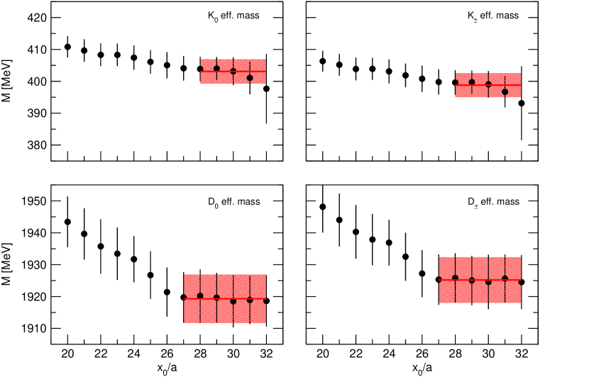
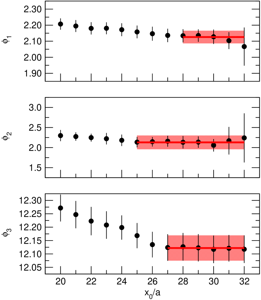
Figure 4: Meson effective masses and effective $\phi$ observables for the ensemble A380a07b324+RW1, together with the selected plateaux and the fits to a constant. Values in MeV are obtained by using the reference value $(8t_{0})^{1/2}=0.415\text{ fm}$ [19].

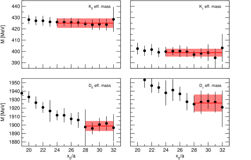
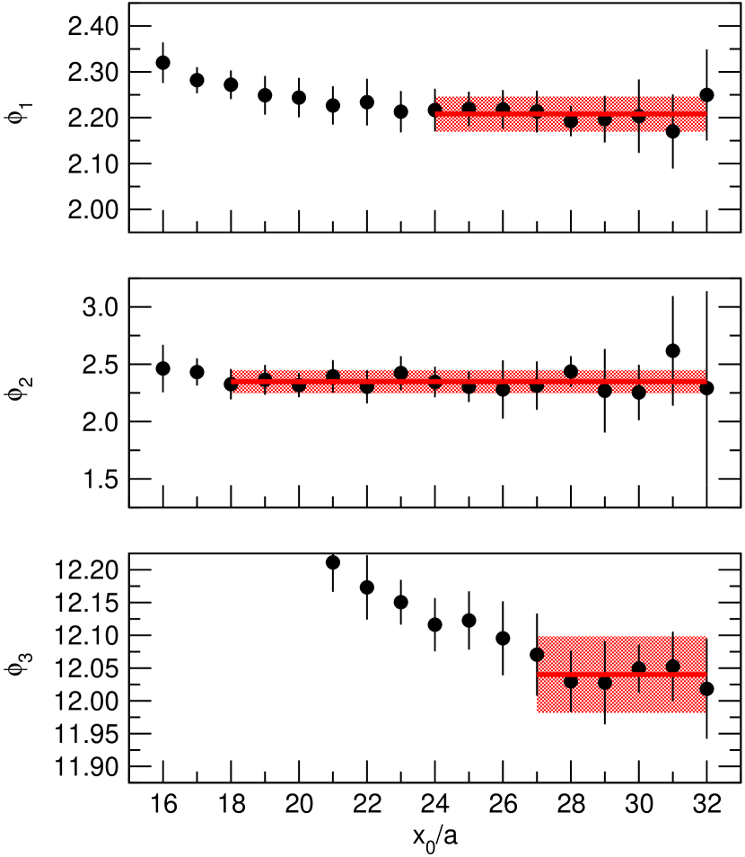
Figure 5: Meson effective masses and effective $\phi$ observables for the ensemble A360a50b324+RW2, together with the selected plateaux and the fits to a constant. Values in MeV are obtained by using the reference value $(8t_{0})^{1/2}=0.415\text{ fm}$ [19].

4.3 Baryon masses

Baryon interpolating operators are written in terms of Gaussian-smeared fermion fields defined by

$$\Psi_{\text{(s)}}=(1+\omega H)^{n}\Psi\ ,\qquad\bar{\Psi}_{\text{(s)}}=\bar{\Psi}(1+\omega H)^{n}\ ,$$ (4.28)

where $\Psi$ and $\bar{\Psi}$ are the dressed fermion fields defined in eq. (4.22), $\omega$ and $n$ are adjustable parameters, and $H$ is the spatial hopping operator given by

$$H\Psi(x)=\sum^{3}_{k=1}\left\{V(x,k)\Psi(x+a\hat{e}_{k})+V(x-a\hat{e}_{k},k)^{\dagger}\Psi(x-a\hat{e}_{k})\right\}\ .$$ (4.29)

In this formula $V$ is an SU(3) smeared link variable. In practice, we construct $V$ by means of a generalization of the gradient flow restricted to a single time slice, i.e. we solve a dicretized version of the following differential equation

$$\partial_{s}U_{s}(x,k)=\partial_{x,k}\sum_{i\neq j}\operatorname{tr}P_{s,ij}(x)\ ,$$ (4.30)

where $P_{s,ij}(x)$ is the plaquette in $x$ on the plane identified by the indices $(i,j)$, constructed with the field $U_{s}$, and the initial condition $U_{0}=U$ is used. The smeared field $V$ is identified with $U_{s}$ at the chosen maximum value of the auxiliary flowtime $s$. We notice that the smeared fields are local in time and invariant under U(1) gauge transformations.

For definiteness we consider the chiral representation of the gamma matrices and $C=i\gamma_{0}\gamma_{2}$. The C-even zero-momentum interpolating operators for spin-1/2 baryons considered in this work can be all written in the form

$$B(x_{0})=\sum_{\mathbf{x}}\sum_{\begin{subarray}{c}abc\\ fgh\end{subarray}}\epsilon_{abc}F_{fgh}$$ (4.31)

$$\hskip 51.21495pt\times\left\{\Psi_{\text{(s)}fa}\Psi_{\text{(s)}gb}^{t}C\gamma_{5}\Psi_{\text{(s)}hc}(x_{0},\mathbf{x})-C\bar{\Psi}^{t}_{\text{(s)}fa}\bar{\Psi}_{\text{(s)}gb}C\gamma_{5}\bar{\Psi}^{t}_{\text{(s)}hc}(x_{0},\mathbf{x})\right\}\ ,$$

where $a,b,c$ are colour indices and $f,g,h$ are flavour indices (spin indices are implicit or contracted). Different baryons are obtained by choosing particular tensors $F_{fgh}$, according to the table 11. In this case the zero-momentum two-point function is defined as

$$C(x_{0})=\langle B^{t}(0)C\frac{1+\gamma_{0}}{2}B(x_{0})\rangle\ .$$ (4.32)

For the $\Omega^{-}$ baryon we use the following C-even zero-momentum interpolating operator

$$\Omega_{j}(x_{0})=\sum_{\mathbf{x}}\sum_{abc}\sum_{k}\epsilon_{abc}\left(\delta_{jk}-\tfrac{1}{3}\gamma_{j}\gamma_{k}\right)$$ (4.33)

$$\hskip 51.21495pt\times\left\{S_{\text{(s)}a}S_{\text{(s)}b}^{t}C\gamma_{k}S_{\text{(s)}c}(x_{0},\mathbf{x})-C\bar{S}^{t}_{\text{(s)}a}\bar{S}_{\text{(s)}b}\gamma_{k}C\bar{S}^{t}_{\text{(s)}c}(x_{0},\mathbf{x})\right\}\ ,$$

where $S_{\text{(s)}}=\Psi_{\text{(s)}s}$ is the smeared dressed field of the strange quark. In this case the zero-momentum two-point function is defined as

$$C(x_{0})=\sum_{j}\langle\Omega^{t}_{j}(0)C\frac{1+\gamma_{0}}{2}\Omega_{j}(x_{0})\rangle\ .$$ (4.34)

In practice we use point sources to calculate the needed two-point functions. For each configuration we construct $12h$ point sources (running over each color and spin index, and located at $h$ random timeslices), where $h=8$ for all ensembles except A500a50b324 and A360a50b324+RW2 for which we have used $h=4$. We used the Generalized Eigenvalue Problem [35, 36] to optimize the smearing parameters. The results given in this paper use a smearing $s=3.6$, $n=400$ and $\omega=0.5$ for the source and no smearing for the sink. Because of the boundary conditions quark-quark and antiquark-antiquark Wick contractions do not vanish (but are exponentially suppressed with the volume). In this work we have simply neglected these Wick contractions which effectively means that we are calculating the two-point function of some partially-quenched baryons as discussed in section 3.3. We plan to quantify the contribution of the extra Wick contractions in future work.

$(1/2)^{+}$ Baryon	Non-zero components of $F_{fgh}$
p	$F_{uud}=1$
n	$F_{ddu}=1$
$\Lambda_{0}$	$F_{sud}=2$, $F_{dus}=1$, $F_{uds}=-1$
$\Sigma^{+}$	$F_{uus}=1$
$\Sigma^{-}$	$F_{dds}=1$
$\Xi_{0}$	$F_{ssu}=1$
$\Xi^{-}$	$F_{ssd}=1$

Table 11: Flavour tensor $F_{fgh}$ defining the interpolating operators for spin-$1/2$ baryons via eq. (4.31). The flavour indices can take values $u$, $d$, $s$, $c$.

Given the zero-momentum two-point function $C(x_{0})$, we define the effective mass $M(x_{0})$ simply as:

$$M(x_{0})=\frac{1}{a}\log\frac{C(x_{0})}{C(x_{0}+a)}\ .$$ (4.35)

The effective mass $M_{c}(x_{0})$ corrected for structure-independent finite-volume effects is defined as for the mesons using eq. (4.27). A selection of effective masses and mass differences with the corresponding plateau fits are shown in figures 6 and 7.

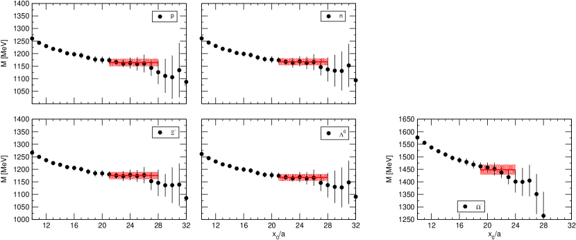
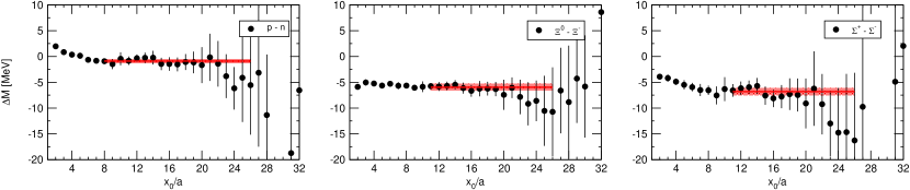
Figure 6: Baryon effective masses for the ensemble A380a07b324+RW1, with the selected plateaux and the fits to a constant. Values in MeV are obtained by using the reference value $(8t_{0})^{1/2}=0.415\text{ fm}$ [19].

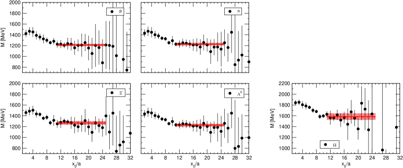
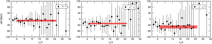
Figure 7: Baryon effective masses and effective $\phi$ observables for the ensemble A360a50b324+RW2, with the selected plateaux and the fits to a constant. Values in MeV are obtained by using the reference value $(8t_{0})^{1/2}=0.415\text{ fm}$.

4.4 Tuning strategy

For fixed values of $\alpha$ and $\beta$, the bare quark masses need to be tuned to obtain the desired values of the $\phi$ variables given by eq. (2.4). Since we have chosen to work with $m_{d}=m_{s}\equiv m_{ds}$, this is a three-parameter tuning problem. In practice, we have followed the following steps:

1. Generate some ensembles with smaller statistics ($\sim$200 thermalized configurations), and get a rough estimate $\hat{m}^{(0)}=(m_{u}^{(0)},m_{ds}^{(0)},m_{c}^{(0)})$ for the quark masses.

2. Generate an ensemble with full statistics (at least 1000 thermalized configurations) with quark masses equal to $\hat{m}^{(0)}$. Calculate the values of the $\phi^{(0)}=(\phi^{(0)}_{1},\phi^{(0)}_{2},\phi^{(0)}_{3})$ observables on these configurations.

3. Choose three new sets of quark masses $\hat{m}^{(i)}$ with $i=1,2,3$ fairly close to $\hat{m}^{(0)}$, and calculate the values of the $\phi^{(i)}$ observables corresponding to these quark masses, by means of mass reweighting. Find the tuned values of the quark masses $\hat{m}^{(t)}$ by linear interpolation, i.e. by assuming that the $\phi$ observables depend on the masses $\hat{m}$ as in $\phi=A\hat{m}+b$, where $A$ is a $3\times 3$ matrix and $b$ is a $3$-vector. A few attempts may be necessary in order to find values for $\hat{m}^{(i)}$ for which the reweighting does not have an overlap problem, and for which the tuned value is found either by interpolation or by a mild extrapolation.

4. Generate an ensemble with full statistics (2000 thermalized configurations) with quark masses equal to $\hat{m}^{(t)}$. Calculate the values of the $\phi^{(t)}$ observables on these configurations.

5. If the extrapolation in point 2 is too long, then one does not get the target value for the $\phi$ observables, and one needs to repeat everything from step 2 with $\hat{m}^{(0)}\leftarrow\hat{m}^{(t)}$. On the other hand, some residual small mistuning due to the linear approximation is corrected by repeating step 2 with $\hat{m}^{(0)}\leftarrow\hat{m}^{(t)}$. In this case a corrected tuned value $\hat{m}^{(t)}$ is found, and the observables are calculated by mass reweighting to the corrected tuned value, without generating new configurations.

In this paper we describe all ensembles with full statistics that we have generated in the tuning procedure, but not all intermediate mass reweighting factors.

It is worth noticing that we have tried carrying out step 2 by changing only the valence quark masses, i.e. without including a mass reweighting factor. However, we usually incurred into a problem of overshooting which rendered this strategy unusable. Nevertheless, if one starts from a value of $\hat{m}^{(0)}$ which is far away from the target value, a first tuning iteration performed by changing only the valence quark masses can be a relatively inexpensive way to move towards the correct region of parameter space.

4.5 Statistical analysis

Errors are calculated with the gamma method in the particular incarnation of [37]. The integrated autocorrelation time is calculated first with the Wolff’s automatic windowing procedure [38] with parameter $S=1$. Among all considered observables $t_{0}/a^{2}$ has the largest integrated autocorrelation time and we use this as an estimate of the exponential autocorrelation time $\tau_{\text{exp}}$, which is a property of the particular Markov chain rather than of the observable. For each observable the autocorrelation function $\Gamma(t)$ is calculated from data for $t=0,1,\dots,\bar{t}$, where $\bar{t}$ is chosen in such a way that the central value of $\Gamma(t)$ is positive for any $t\leq\bar{t}$ and negative for $t=\bar{t}+1$. Then the autocorrelation function is extended for $t>\bar{t}$ with a single exponential $\Gamma(t)=\Gamma(\bar{t})\exp[-(t-\bar{t})/\tau_{\text{exp}}]$. The extended autocorrelation function is used in the gamma method to calculate errors and integrated autocorrelation times. The analysis has been carried out with our own code, which implements the ideas of [39].

4.6 Sign of the pfaffian

Given a quark field $\psi$, we introduce the corresponding antiquark field $\psi^{\mathcal{C}}=C^{-1}\bar{\psi}^{t}$, where the charge-conjugation matrix $C$ can be chosen to be $i\gamma_{0}\gamma_{2}$ in the chiral basis. C^⋆ boundary conditions for the fermion fields can be written as

$$\begin{pmatrix}\psi(x+L\hat{k})\\ \psi^{\mathcal{C}}(x+L\hat{k})\end{pmatrix}=\begin{pmatrix}\psi^{\mathcal{C}}(x)\\ \psi(x)\end{pmatrix}\equiv K\begin{pmatrix}\psi(x)\\ \psi^{\mathcal{C}}(x)\end{pmatrix}\ .$$ (4.36)

With C^⋆ boundary conditions the Dirac operator $D$ acts on the quark-antiquark doublet in a non-diagonal way, and it is therefore a $24V\times 24V$ matrix, where $V=TL^{3}/a^{4}$. An explicit representation for the Dirac operator is given in appendix A. The integration of a quark field in the path integral yields the pfaffian $\operatorname{pf}(CKD)$ in place of the standard fermionic determinant, where $CKD$ is an antisymmetric matrix (see proposition 1 in appendix A). The absolute value of the pfaffian is given by

$$\left|\operatorname{pf}(CKD)\right|=\left|\det D\right|^{1/2}\ ,$$ (4.37)

and can be simulated by means of a standard RHMC algorithm, while the sign of the pfaffian can be incorporated as a reweighing factor.

In order to calculate this sign, it is convenient to relate the pfaffian to the spectrum of the hermitian Dirac operator $Q=\gamma_{5}D$. It turns out that the spectrum of $Q$ is doubly degenerate (see proposition 2 in appendix A). Let $\lambda_{n=1,\dots,12V}\in\mathbb{R}$ be the list of eigenvalues of $Q$, each of them appearing a number of times equal to half their degeneracy. The following simple formula holds (see proposition 3 in appendix A):

$$\operatorname{pf}(CKD)=\prod_{n=1}^{12V}\lambda_{n}\ .$$ (4.38)

It follows that the pfaffian is positive (resp. negative) if the number of negative eigenvalues $\lambda_{n}$ is even (resp. odd). In practice, we calculate the sign by following the eigenvalue flow as a function of the quark mass $m$. We use the crucial fact that the eigenvalues of $Q(m)$ can be labeled in such a way that they are continuous functions of $m$. As $m$ is continuously varied, the pfaffian flips sign every time a degenerate pair of eigenvalues of $Q(m)$ crosses zero. It follows that

$$\operatorname{sgn}\operatorname{pf}[CKD(m)]=(-1)^{c(m,M)}\operatorname{sgn}\operatorname{pf}[CKD(M)]\ ,$$ (4.39)

where we have highlighted the mass dependence of the Dirac operator, and $c(m,M)$ is the number of degenerate pairs of eigenvalues of $Q(m)$ crossing zero as the mass is continuously varied from $m$ to $M$.

If $M$ is chosen very large, then $Q(M)$ is approximately equal to $M\gamma_{5}$ and the number of negative $\lambda_{n}$’s is even and equal to $6V$. Hence, the pfaffian of $CKD(M)$ is positive, and eq. (4.39) implies that the sign of the pfaffian of $CKD(m)$ can be calculated by counting the number of eigenvalue pairs crossing zero between the target mass $m$ and some large mass $M$: the pfaffian is positive if this number is even and negative otherwise.

In the particular case of QCD+QED simulations with 4 flavours we use the following observation to eliminate the arbitrariness associated to the choice of $M$. If $D_{+2/3}(m)$ is the Dirac operator for a quark with electric charge $+2/3$, then the Dirac operators for the up and charm quarks are simply $D_{u}=D_{+2/3}(m_{u})$ and $D_{c}=D_{+2/3}(m_{c})$, since the two quarks differ only for their mass. Using eq. (4.39), one gets the contribution to the sign of up and charm quarks as:

$$\operatorname{sgn}\operatorname{pf}(CKD_{u})\,\operatorname{sgn}\operatorname{pf}(CKD_{c})=(-1)^{c_{+2/3}(m_{u},m_{c})}\ ,$$ (4.40)

where the subscript of $c_{+2/3}$ stresses the fact that we need to count the eigenvalue crossings of the hermitian Dirac operator for a quark with electric charge $+2/3$. Analogously, the contribution to the sign of down and strange quarks is:

$$\operatorname{sgn}\operatorname{pf}(CKD_{d})\,\operatorname{sgn}\operatorname{pf}(CKD_{s})=(-1)^{c_{-1/3}(m_{d},m_{s})}\ .$$ (4.41)

The reweighting factor needed to account for the sign of the fermionic pfaffian is then given by:

$$W_{\text{sgn}}=\prod_{f=u,d,s,c}\operatorname{sgn}\operatorname{pf}(CKD_{f})=(-1)^{c_{+2/3}(m_{u},m_{c})}(-1)^{c_{-1/3}(m_{d},m_{s})}\ .$$ (4.42)

At the U-symmetric point $m_{d}=m_{s}$ one has trivially $c_{-1/3}(m_{d},m_{s})=0$, and one only needs to count the number of eigenvalue crossings for up-type quarks as the mass is varied from the up-quark mass to the charm-quark mass.

We give a brief account of the techniques used in this work to calculate $c(m,M)$, i.e. to count the number of eigenvalue crossings of $Q$ as the mass is varied continuously form $m$ to $M$. Our method is based on two stages:

1. A first fast algorithm finds an interval $I\subset[m,M]$ in the considered range of bare masses, with the property that no sign flip occurs in the complement of $I$. Typically $I$ is much smaller in length than the original $[m,M]$, and for most configurations $I$ turns out to be empty.

2. If $I$ is not empty, we follow the flow of a certain number of eigenvalues which are the closest to zero, only inside the typically small interval $I$, using the methods described in [40, 14]. By tracking the eigenvalues as functions of the mass, we can determine whether a sign flip occurs.

To the best of our knowledge, the first step of our method has never been used in similar calculations. Since it speeds up significantly the calculation of the sign of fermionic pfaffian, and it can be used also in different contexts (e.g. for the calculation of the sign of the fermionic determinant in QCD, or the sign of the fermionic pfaffian in gauge theories with adjoint fermions), we discuss it here in some detail.

The starting point is the following simple observation. Let $\mu(m)$ be the smallest eigenvalue of $|Q(m)|$, i.e.

$$\mu(m)=\min_{n}|\lambda_{n}(m)|\ .$$ (4.43)

If $\bar{\mu}\equiv\mu(\bar{m})>0$, then no eigenvalue $\lambda_{n}(m)$ flips sign as long as $m$ is in the interval defined by $|m-\bar{m}|<\bar{\mu}$.

Proof.

We use the notation $m=\bar{m}+\delta m$. Let $v$ be a normalized vector. Using the identity $Q(m)=Q(\bar{m})+\delta m\,\gamma_{5}$, the triangular inequality and the unitarity of $\gamma_{5}$, one readily derives

$$\left\|Q(m)v\right\|\geq\left\|Q(\bar{m})v\right\|-|\delta m|\,\left\|\gamma_{5}v\right\|=\left\|Q(\bar{m})v\right\|-|\delta m|\geq\bar{\mu}-|\delta m|\ .$$ (4.44)

In the last step we have also used the fact that $\bar{\mu}$ is the smallest eigenvalue of $|Q(\bar{m})|$. If we choose for $v$ any of the eigenvectors of $Q(m)$, the above inequality specializes to

$$|\lambda_{n}(m)|\geq\bar{\mu}-|\delta m|\ .$$ (4.45)

If $|m-\bar{m}|=|\delta m|<\bar{\mu}$ then $|\lambda_{n}(m)|>0$. Since $\lambda_{n}(m)$ is continuous in $m$, it is either always positive or always negative in the interval defined by $|m-\bar{m}|<\bar{\mu}$.

∎

This result allows us to design the following iterative algorithm which restricts the original interval $I=[m,M]$, in which we search for sign flips, to the interval $I^{\prime}=[m^{\prime},M]$ constructed in the following way:

1. Set $m_{0}=m$ and $n=0$.

2. Define $\mu_{n}$ to be a safe non-negative lower bound for $\mu(m_{n})$. The lowest eigenvalue of $|Q(m_{n})|$ can be calculated with a standard power method applied to $Q(m_{n})^{-2}$.

3. Since no sign flip occurs in $[m_{n},m_{n}+\bar{\mu}_{n})$, we set $m_{n+1}=m_{n}+(1-\epsilon)\bar{\mu}_{n}$. $\epsilon$ is a tunable small positive parameter which we choose to be 0.1.

4. If $m_{n+1}-m_{n}<\eta m_{n}$ or $m_{n+1}>M$, we set $m^{\prime}=m_{n+1}$ and we stop the algorithm, otherwise we repeat from 2 with $n\leftarrow n+1$. $\eta$ is a tunable parameter satisfying $0<\eta<1$, which we choose to be 1/4.

For most configurations, $\mu_{n}$ is an increasing sequence. In this situation this part of the algorithm covers the whole interval in a handful of steps, as illustrated in figure 8. If the interval $I^{\prime}=[m^{\prime},M]$ is not empty, we restrict it to a new interval $I^{\prime\prime}=[m^{\prime},M^{\prime}]$ constructed in the following way:

1. Set $M_{0}=M$ and $n=0$.

2. Define $\mu_{n}$ to be a safe non-negative lower bound for $\mu(M_{n})$.

3. Since no sign flip occurs in $(M_{n}-\bar{\mu}_{n},M_{n}]$, we set $M_{n+1}=M_{n}-(1-\epsilon)\bar{\mu}_{n}$.

4. If $M_{n}-M_{m+1}<\eta M_{n}$ or $M_{n+1}<m^{\prime}$, we set $M^{\prime}=M_{n+1}$ and we stop the algorithm, otherwise we repeat from 2 with $n\leftarrow n+1$.

If the interval $I^{\prime\prime}=[m^{\prime},M^{\prime}]$ is not empty, then one resorts to the methods described in [40, 14]. In this case, one tracks the mass-dependence of eigenvalues and eigenvectors in the interval $I^{\prime\prime}$. Since a fairly accurate determination of eigenvectors is required for a fairly fine scan of the mass, this stage of the algorithm is intrinsically more expensive than the previous one. However, in practice, it needs to be applied only to a relatively small number of configurations and to small mass intervals.

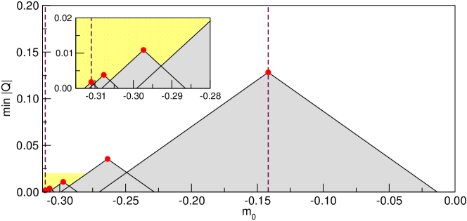
Figure 8: Smallest eigenvalue of $|Q|$ for up-type quarks as a function of the valence mass $m_{0}$ (red points), calculated on a representative configuration (C380a50b324 ensemble). Using the bound (4.44), one proves that $|Q|$ has no eigenvalues in the grey areas. This implies that no eigenvalue of $Q$ crosses zero between the up-quark mass (left dashed vertical line) and the charm-quark mass (right dashed vertical line). One can see that we are able to flow the lowest eigenvalue across two orders of magnitude in only five steps. The inset is a zoom-in of the yellow area.

4.7 Algorithmic parameters

In this section we report on the algorithmic parameters chosen to generate the presented gauge configurations, with a particular emphasis on integration scheme, solvers and rational approximations.

Rational approximations

Because of C^⋆ boundary conditions, we need to simulate the following fermionic determinant

$$\det(\hat{D}_{u}^{\dagger}\hat{D}_{u})^{1/4}\det(\hat{D}_{ds}^{\dagger}\hat{D}_{ds})^{1/2}\det(\hat{D}_{c}^{\dagger}\hat{D}_{c})^{1/4}$$ (4.46)

for the QCD+QED ensembles ($\alpha\neq 0$, $m_{d}=m_{s}$) and the following fermionic determinant

$$\det(\hat{D}_{uds}^{\dagger}\hat{D}_{uds})^{3/4}\det(\hat{D}_{c}^{\dagger}\hat{D}_{c})^{1/4}$$ (4.47)

for the QCD ensembles ($\alpha=0$, $m_{u}=m_{d}=m_{s}$). Here $\hat{D}$ denotes the even-odd preconditioned Dirac operator. The inverse operators $(\hat{D}^{\dagger}\hat{D})^{-\gamma}$ with $\gamma=1/4,1/2,3/4$ are approximated with rational functions of $\hat{D}^{\dagger}\hat{D}$.

In practice, we construct the rational function $R(x)$ of order $(N,N)$ that minimizes the relative precision, i.e. the maximum of $|1-x^{\gamma}R(x)|$ over some interval $x\in[r_{a}^{2},r_{b}^{2}]$. The approximation range is chosen in such a way that the eigenvalues of $\hat{D}^{\dagger}\hat{D}$ are included in $[r_{a}^{2},r_{b}^{2}]$ most of the time. In table 12 we report the parameters defining the rational approximations used for this work.

The error introduced by the rational approximation is corrected by means of a reweighting factor. This strategy is identical to the one adopted in the openQCD code [41]. The generalization to any value of $\gamma$ of the reweighting factor can be found in [26]. The parameters of the rational functions have been chosen in such a way that the reweighting factor does not introduce any detectable increase in the errors of the considered observables.

When a rational approximation is used, the Dirac operator always appears in the pseudofermion actions in the combination $\hat{D}^{\dagger}\hat{D}+\mu^{2}$ for strictly positive values of $\mu$. The rational approximation has the effect of removing the infinite potential barrier encountered when the fermionic determinant or pfaffian tries to change sign [14], pretty much in the same way as the twisted-mass reweighting procedure proposed in [42]. However, if the ratio $r_{b}/r_{a}$ becomes too large or if the precision of the rational approximation is chosen to be too high, then the smallest twisted mass $\mu$ becomes too small, and the potential barrier may become large enough to jeopardize ergodicity and stability of the algorithm. For this reason we have progressively reduced the precision of the rational approximations used in our runs, settling for a precision of a few units of $10^{-6}$ in our latest runs.

Pseudofermion actions and solvers

For a given flavour, the approximated determinant $\det R^{-1}$ is represented by means of a sum of pseudofermion actions in the following way. We start from the rational function

$$R=A\prod_{k=1}^{N}\frac{\hat{D}^{\dagger}\hat{D}+\nu_{k}^{2}}{\hat{D}^{\dagger}\hat{D}+\mu_{k}^{2}}\ .$$ (4.48)

In the following we assume the ordering $\nu_{1}<\nu_{2}<\dots<\nu_{N}$ and $\mu_{1}<\mu_{2}<\dots<\mu_{N}$. We introduce a pseudofermion action for each factor in the above equation with $k=1,\dots,N_{2}$, and a single pseudofermion action for the remaining factors, i.e.

$$S_{k}=\phi_{k}^{\dagger}\frac{\hat{D}^{\dagger}\hat{D}+\nu_{k}^{2}}{\hat{D}^{\dagger}\hat{D}+\mu_{k}^{2}}\phi_{k}\ ,\qquad\text{for }k=1,\dots,N_{2}\ ,$$ (4.49)

$$S_{N_{2}+1}=\phi_{N_{2}+1}^{\dagger}\left(\prod_{k=N_{2}+1}^{N}\frac{\hat{D}^{\dagger}\hat{D}+\nu_{k}^{2}}{\hat{D}^{\dagger}\hat{D}+\mu_{k}^{2}}\right)\phi_{N_{2}+1}\ .$$ (4.50)

In practice, the pseudofermion actions are represented by means of partial fraction decompositions as explained in [43]. The chosen values for $N_{2}$ are reported in table 12.

One needs to invert the operator $(\hat{D}+i\mu_{k})$ in the calculation of the pseudofermion actions, and the operator $(\hat{D}+i\nu_{k})$ in the generation of the pseudofermion fields. The multishift conjugate gradient is used for the pseudofermion action $S_{N_{2}+1}$, while a deflated generalized conjugate residual method [44], preconditioned with the Schwarz alternating procedure [45], is used for all other pseudofermion actions. We use a $10^{-8}$ residue for all solvers used in the calculation of the force, and a $10^{-10}$ residue for all solvers used in the calculation of the action and in the generation of the pseudofermion fields.

A distinctive feature of the QCD+QED simulations is the need for different deflation subspaces for different values of the electric charge ($\hat{q}=2,4$ in our simulations). Using the notation of the openQ*D input files [43], we used $\texttt{mu}=0.001$ for the $64\times 32^{3}$ lattices and $\texttt{mu}=0.005$ for the other ones, $\texttt{nkr}\geq 24$, and a total of $\texttt{Ns}=20$ deflation vectors. The size of the deflation blocks have been chosen to be as large as possibile, compatibly with the size of the local lattice and the constraints of the simulation code.

HMC parameters and integration of Molecular Dynamics

The sum of the gauge and pseudofermion actions is simulated with the Hybrid Monte Carlo (HMC) algorithm with Fourier acceleration for the U(1) field [46, 47]. The Molecular Dynamics (MD) equations are solved by means of a symplectic multilevel integrator [48]. We use a MD trajectory length $\tau=2$ and a three-level scheme for all our simulations. For each level one needs to specify: the number of integration steps, the forces to be integrated and the type of integrator.

The fermionic forces corresponding to the pseudofermion actions $S_{k}$ with $k=1,\dots,N_{1}$ (with $N_{1}\leq N_{2}$) are integrated in the outermost level with the Omelyan–Mryglod–Folk (OMF) [49] second-order integrator. All other fermionic forces are integrated in the intermediate level with the OMF fourth-order integrator. Finally, the gauge forces are integrated in the innermost level with the OMF fourth-order integrator. The chosen values for $N_{1}$ and also the number of steps for each integration level are reported in table 12.

ensemble	int. steps	flavours	$\gamma$	$[r_{a},r_{b}]$	$N$ [prec.]	$N_{1}$	$N_{2}$
A400a00b324	(1,1,8)	uds	3/4	[0.00132,8.0]	18 [4.02e-08]	6	10
		c	1/4	[0.25500,8.0]	8 [7.97e-08]	0	0
B400a00b324	(1,1,16)	uds	3/4	[0.00132,8.0]	18 [4.02e-08]	6	10
		c	1/4	[0.25500,8.0]	8 [7.97e-08]	0	0
A450a07b324	(1,1,12)	u	1/4	[0.0004,10.0]	15 [4.73e-06]	5	8
		ds	1/2	[0.0010,10.0]	14 [5.46e-06]	4	7
		c	1/4	[0.2000,10.0]	7 [2.36e-06]	0	0
A380a07b324	(1,1,12)	u	1/4	[0.0020,10.0]	13 [4.00e-06]	3	6
		ds	1/2	[0.0010,10.0]	13 [1.38e-05]	3	6
		c	1/4	[0.2000,10.0]	7 [2.36e-06]	0	0
A500a50b324	(1,1,12)	u	1/4	[0.00070,9.0]	15 [2.09e-06]	5	8
		ds	1/2	[0.00132,9.0]	15 [1.25e-06]	5	8
		c	1/4	[0.20000,8.0]	9 [1.84e-08]	0	0
A360a50b324	(1,1,12)	u	1/4	[0.0004,10.0]	15 [4.73e-06]	5	8
		ds	1/2	[0.0010,10.0]	14 [5.46e-06]	4	7
		c	1/4	[0.2000,10.0]	7 [2.36e-06]	0	0
C380a50b324	(1,1,18)	u	1/4	[0.0004,10.0]	15 [4.73e-06]	5	8
		ds	1/2	[0.0010,10.0]	14 [5.46e-06]	4	8
		c	1/4	[0.2000,10.0]	7 [2.36e-06]	0	0

Table 12: Parameters defining the integration scheme and the pseudofermion actions. In the second column (int. steps) we report the number of integration steps for the innermost, intermediate and outermost integration levels. For each degenerate multiplet of quarks specified in the third column (flavours), we use a rational approximation for the operator $(\hat{D}^{\dagger}\hat{D})^{-\gamma}$. We report the exponent $\gamma$, the chosen range $[r_{a},r_{b}]$, the order $(N,N)$ of the rational approximation, and its relative uniform precision. $N_{1}$ denotes the number of factors integrated in the outermost level of the integrator, and $N_{2}$ denotes the number of factors that have been split into independent pseudofermion actions.

5 Outlook

We have presented seven (two QCD and five QCD+QED) gauge ensembles with C^⋆ boundary conditions. Three different values of the renormalized fine-structure constant ($\alpha_{R}\simeq 0,1/137,0.04$) and two different volumes ($L\simeq 1.6\text{ fm},2.4\text{ fm}$) have been considered. In all cases we have simulated close to the SU(3)-symmetric point: in particular the simulated up and down quarks are heavier than the physical ones, and the simulated strange quark is lighter than the physical one. We have calculated a number of observables: pseudoscalar meson masses, octet baryon masses, and the $\Omega^{-}$ mass, the flow scale $t_{0}$ and the renormalized fine-structure constant in the gradient-flow scheme. While this is only the first step of a long-term research project, we comment here only on our goal for the near future.

Baryon masses are unsurprisingly very noisy. Since the $\Omega^{-}$ is needed to set the scale in our simulations, we plan to implement state-of-the-art noise-reduction techniques and to invest significant resources in order to bring the error down. In baryon correlators, we have also neglected the quark-disconnected contractions, which are peculiar of C^⋆ boundary conditions. This is equivalent to calculating the masses of some partially-quenched baryons which become degenerate with the physical baryons in the infinite-volume limit. We plan to investigate the impact of the disconnected contributions in detail.

The sheer number of parameters in QED+QCD simulations makes the tuning particularly expensive. We have presented a tuning strategy, based on a number of tricks which include mass-reweighting and linear interpolations and extrapolations in parameters space. It turns out that on the smaller volumes, there is no point in pushing the precision of the tuning too much, since finite-volume effects are still significant. Volumes larger than the ones presented here will need to be simulated in order to gain better control on finite-volume effects. However, a first analysis already indicates that finite-volume effects are smaller than the statistical errors on the larger volume presented in this paper.

We also want to move towards physical quark masses, by making the up and down quarks lighter, and the strange quark heavier. Besides the obvious phenomenological motivation, it will be interesting to see how the cost of simulations changes when the up quark gets lighter.

Acknowledgements

We are grateful to Anian Altherr, Roman Gruber, Javad Komijani, Sofie Martins, Paola Tavella for detailed feedback on the paper and useful conversations. Alessandro Cotellucci and Jens Lücke’s research is funded by the Deutsche Forschungsgemeinschaft (DFG, German Research Foundation) - Projektnummer 417533893/GRK2575 “Rethinking Quantum Field Theory”. The funding from the European Union’s Horizon 2020 research and innovation program under grant agreement No. 813942 and the financial support by SNSF (Project No. 200021_200866) is gratefully acknowledged. The authors gratefully acknowledge the computing time granted by the Resource Allocation Board and provided on the supercomputer Lise and Emmy at NHR@ZIB and NHR@Göttingen as part of the NHR infrastructure. The calculations for this research were partly conducted with computing resources under the project bep00085 and bep00102. The work was supported by CINECA that granted computing resources on the Marconi supercomputer to the LQCD123 INFN theoretical initiative under the CINECA-INFN agreement. The authors acknowledge access to Piz Daint at the Swiss National Supercomputing Centre, Switzerland under the ETHZ’s share with the project IDs go22, go24, eth8, and s1101. The work was supported by the Poznan Supercomputing and Networking Center (PSNC) through grant numbers 450 and 466.

Appendix A Properties of the pfaffian

In this appendix we review the main properties of the Dirac operator and its pfaffian. We use here $a=1$. The Dirac operator acts on the quark-antiquark doublet

$$\chi=\begin{pmatrix}\psi\\ \psi^{\mathcal{C}}\end{pmatrix}=\begin{pmatrix}\psi\\ C^{-1}\bar{\psi}^{t}\end{pmatrix}\ ,$$ (A.51)

and can be written as a sum of terms

$$D=m+D_{\mathrm{w}}+\delta D_{\mathrm{sw}}\ .$$ (A.52)

The Wilson–Dirac operator has the standard form

$$D_{\mathrm{w}}=\frac{1}{2}\sum_{\mu}\left\{\gamma_{\mu}(\nabla_{\mu}-\nabla_{\mu}^{\dagger})-\nabla_{\mu}^{\dagger}\nabla_{\mu}\right\}\ ,$$ (A.53)

but the forward covariant derivative $\nabla_{\mu}$ is constructed keeping in mind that the quark and antiquark fields transform under different representations of the gauge group, one being the complex conjugate of the other, i.e.

$$\nabla_{\mu}\chi(x)=\begin{pmatrix}z^{\hat{q}}(x,\mu)U(x,\mu)&0\\ 0&z^{-\hat{q}}(x,\mu)U^{*}(x,\mu)\end{pmatrix}\chi(x+\hat{\mu})-\chi(x)\ ,$$ (A.54)

where $U(x,\mu)$ and $z(x,\mu)$ are the SU(3) and U(1) link variables, and $\hat{q}$ is the electric charge of the quark in units of $q_{el}$ which appears in eq. (3.5). With our choice $q_{el}=1/6$, up-type quarks have $\hat{q}=4$ while down-type quarks have $\hat{q}=-2$. In finite volume, the definition of the forward derivative is supplemented with the boundary conditions

$$\chi(x+\tfrac{T}{a}\hat{0})=\chi(x)\ ,\qquad\chi(x+\tfrac{L}{a}\hat{k})=K\chi(x)\ ,$$ (A.55)

for $k=1,2,3$. The matrix

$$K=\begin{pmatrix}0&1\\ 1&0\end{pmatrix}$$ (A.56)

exchanges quark and antiquark, and implements C^⋆ boundary conditions in this formalism. The Sheikholeslami–Wohlert term also takes into account the fact that quark and antiquark fields transform in different representations of the gauge group, and is given explicitly by

$$\delta D_{\mathrm{sw}}=-\frac{1}{4}\sum_{\mu,\nu}\sigma_{\mu\nu}\left\{c_{\mathrm{sw}}^{\mathrm{SU(3)}}\begin{pmatrix}\hat{G}_{\mu\nu}&0\\ 0&-\hat{G}_{\mu\nu}^{*}\end{pmatrix}+\hat{q}\,c_{\mathrm{sw}}^{\mathrm{U(1)}}\begin{pmatrix}\hat{F}_{\mu\nu}&0\\ 0&-\hat{F}_{\mu\nu}^{*}\end{pmatrix}\right\}\ .$$ (A.57)

$\hat{G}_{\mu\nu}$ and $\hat{F}_{\mu\nu}$ are the clover discretizations of the hermitian SU(3) and U(1) field tensors, and $\sigma_{\mu\nu}=\frac{i}{2}[\gamma_{\mu},\gamma_{\nu}]$.

Proposition 1.

The matrix $CKD$ is antisymmetric.

Proof.

For definiteness, we choose to work in the chiral basis for the Euclidean gamma matrices ($\gamma_{5}$ is diagonal, $\gamma_{0,2}$ are real, $\gamma_{1,3}$ are imaginary), and we define the charge conjugation matrix as

$$C=i\gamma_{0}\gamma_{2}\ .$$ (A.58)

Notice that $C$ is imaginary and antisymmetric, and satisfies $C^{2}=1$. Using the gamma matrix identities

$$\gamma_{5}C\gamma_{\mu}C\gamma_{5}=\gamma_{\mu}^{*}\ ,$$ (A.59)

$$\gamma_{5}C\sigma_{\mu\nu}C\gamma_{5}=-\sigma_{\mu\nu}^{*}\ ,$$ (A.60)

and the following identities involving the $K$ matrix

$$K\begin{pmatrix}z^{\hat{q}}U&0\\ 0&z^{-\hat{q}}U^{*}\end{pmatrix}K=\begin{pmatrix}z^{\hat{q}}U&0\\ 0&z^{-\hat{q}}U^{*}\end{pmatrix}^{*}\ ,$$ (A.61)

$$K\begin{pmatrix}\hat{G}_{\mu\nu}&0\\ 0&-\hat{G}_{\mu\nu}^{*}\end{pmatrix}K=-\begin{pmatrix}\hat{G}_{\mu\nu}&0\\ 0&-\hat{G}_{\mu\nu}^{*}\end{pmatrix}^{*}\ ,$$ (A.62)

$$K\begin{pmatrix}\hat{F}_{\mu\nu}&0\\ 0&-\hat{F}_{\mu\nu}^{*}\end{pmatrix}K=-\begin{pmatrix}\hat{F}_{\mu\nu}&0\\ 0&-\hat{F}_{\mu\nu}^{*}\end{pmatrix}^{*}\ ,$$ (A.63)

one easily proves

$$\gamma_{5}CKDKC\gamma_{5}=D^{*}\ ,$$ (A.64)

or, equivalently,

$$CKD=\gamma_{5}D^{*}\gamma_{5}CK=D^{t}CK=-(CKD)^{t}\ .$$ (A.65)

In the third equality we have used $\gamma_{5}$-hermiticity of the Dirac operator, and in the last step we have used $C^{t}=-C$ and $K^{t}=K$.

∎

Proposition 2.

The spectrum of the operator $Q=\gamma_{5}D$ is doubly degenerate.

Proof.

The matrix $U=CK\gamma_{5}$ has the following properties

$$U=U^{\dagger}=U^{-1}=-U^{t}=U^{*}\ .$$ (A.66)

Proposition 1 implies

$$UQ^{*}=CKD^{*}=-(CKD)^{*}=(CKD)^{\dagger}=\gamma_{5}D\gamma_{5}CK=QU\ .$$ (A.67)

As a simple application of the above relations, it follows that:

1. if $v$ is an eigenvector of $Q$ with eigenvalue $\lambda$, then $Uv^{*}$ is also an eigenvector of $Q$ with the same eigenvalue:

   $$QUv^{*}=UQ^{*}v^{*}=U(\lambda v)^{*}=\lambda Uv^{*}\ ,$$ (A.68)

   where the last equality follows from the fact that $\lambda$ is real;

2. $v$ and $Uv^{*}$ are orthogonal:

   $$(Uv^{*},v)=v^{t}U^{\dagger}v=v^{t}Uv=0\ ,$$ (A.69)

   where the last equality follows from the fact that $U$ is antisymmetric;

3. if $w$ is orthogonal to $v$ and $Uv^{*}$, then $Uw^{*}$ is also orthogonal to $v$ and $Uv^{*}$:

   $$(Uw^{*},v)=w^{t}Uv=-v^{t}Uw=-(v^{*},Uw)=-(Uv^{*},w)=0\ ,$$ (A.70)

   $$(Uw^{*},Uv^{*})=w^{t}U^{2}v^{*}=v^{\dagger}w=(v,w)=0\ .$$ (A.71)

A straightforward modification of the Gram–Schmidt algorithm, in which one alternates an orthogonalization step with the construction of an eigenvector of the form $Uv_{i}^{*}$, allows to prove that the degeneracy $d$ of any eigenvector is even, and an orthonormal basis for the corresponding eigenspace can be chosen of the form:

$$v_{1},\ Uv_{1}^{*},\ v_{2},\ Uv_{2}^{*},\ \dots\ ,\ v_{d/2},\ Uv_{d/2}^{*}\ .$$ (A.72)

∎

Proposition 3.

Let $\lambda_{n=1,\dots,12V}\in\mathbb{R}$ be the list of eigenvalues of $Q$, each of them appearing a number of times equal to half their degeneracy. Then the following formula holds

$$\operatorname{pf}\,(CKD)=\prod_{n=1}^{12V}\lambda_{n}\ .$$ (A.73)

Proof.

The pfaffian of a matrix is a polynomial in the entries of the matrix. Since $D$ depends linearly on the bare mass $m$, then the function

$$f(m)=\operatorname{pf}\,[CKD(m)]$$ (A.74)

is a polynomial in $m$. Since $Q$ is hermitian and depends linearly on $m$, for every $m$ its eigenvalues $\lambda_{n}$ can be labeled in such a way that they are analytic functions of $m$ even at level crossings [50]. Then the function

$$g(m)=\prod_{n=1}^{12V}\lambda_{n}(m)$$ (A.75)

is analytical for every real value of $m$.

For $m\to+\infty$ one has $D\simeq mI_{24V}$, which implies

$$\lim_{m\to+\infty}f(m)=\lim_{m\to+\infty}m^{12V}\operatorname{pf}(C\otimes K\otimes I_{3V})=\lim_{m\to+\infty}m^{12V}=+\infty\ .$$ (A.76)

For $m\to+\infty$ one has $Q\simeq mI_{6V}\otimes\gamma_{5}$, which implies that half of the eigenvalues are asymptotically equal to $+m$ and the other half are asymptotically equal to $-m$. Therefore

$$\lim_{m\to+\infty}g(m)=\lim_{m\to+\infty}\prod_{n=1}^{12V}\lambda_{n}=\lim_{m\to+\infty}m^{6V}(-m)^{6V}=+\infty\ .$$ (A.77)

From the two limits it follows that a value $M$ exists such that both $f(m)$ and $g(m)$ are positive for every $m>M$.

Using properties of the pfaffian and the determinant one easily shows that, for every $m$,

$$f(m)^{2}=\operatorname{pf}\,[CKD(m)]^{2}=\det\left[D(m)\right]=\det\left[Q(m)\right]=\prod_{n=1}^{12V}\lambda_{n}^{2}(m)=g(m)^{2}\ .$$ (A.78)

For $m>M$ both functions are positive, therefore the above equality implies $f(m)=g(m)$.

Since $f(m)$ and $g(m)$ are analytic function of $m$, and they are equal for every $m>M$, it follows that they are equal everywhere.

∎

References

- [1] (FLAG), Y. Aoki et al., FLAG Review 2021, 2111.09849.
- [2] A. Patella, QED Corrections to Hadronic Observables, PoS LATTICE2016 (2017) 020, [1702.03857].
- [3] M. A. Clark, M. Della Morte, Z. Hall, B. Hörz, A. Nicholson, A. Shindler et al., QED with massive photons for precision physics: zero modes and first result for the hadron spectrum, PoS LATTICE2021 (2022) 281, [2201.03251].
- [4] T. Blum, N. Christ, M. Hayakawa, T. Izubuchi, L. Jin, C. Jung et al., Using infinite volume, continuum QED and lattice QCD for the hadronic light-by-light contribution to the muon anomalous magnetic moment, Phys. Rev. D 96 (2017) 034515, [1705.01067].
- [5] X. Feng and L. Jin, QED self energies from lattice QCD without power-law finite-volume errors, Phys. Rev. D 100 (2019) 094509, [1812.09817].
- [6] N. H. Christ, X. Feng, L.-C. Jin and C. T. Sachrajda, Finite-volume effects in long-distance processes with massless leptonic propagators, Phys. Rev. D 103 (2021) 014507, [2009.08287].
- [7] B. Lucini, A. Patella, A. Ramos and N. Tantalo, Charged hadrons in local finite-volume QED+QCD with C⋆ boundary conditions, JHEP 02 (2016) 076, [1509.01636].
- [8] (RM123), G. M. de Divitiis, R. Frezzotti, V. Lubicz, G. Martinelli, R. Petronzio, G. C. Rossi et al., Leading isospin breaking effects on the lattice, Phys. Rev. D 87 (2013) 114505, [1303.4896].
- [9] (RC*), I. Campos, P. Fritzsch, M. Hansen, M. Krstić Marinković, A. Patella, A. Ramos et al., Simulation program for lattice QCD+QED: openQ*D code, GitLab: https://gitlab.com/rcstar/openQxD. CSIC: https://dx.doi.org/10.20350/digitalCSIC/8591, https://hdl.handle.net/10261/173334.
- [10] S. Borsanyi et al., Ab initio calculation of the neutron-proton mass difference, Science 347 (2015) 1452–1455, [1406.4088].
- [11] R. Horsley et al., Isospin splittings of meson and baryon masses from three-flavor lattice QCD + QED, J. Phys. G 43 (2016) 10LT02, [1508.06401].
- [12] R. Horsley et al., QED effects in the pseudoscalar meson sector, JHEP 04 (2016) 093, [1509.00799].
- [13] (CSSM, QCDSF, UKQCD), R. Horsley et al., Isospin splittings in the decuplet baryon spectrum from dynamical QCD+QED, J. Phys. G 46 (2019) 115004, [1904.02304].
- [14] D. Mohler and S. Schaefer, Remarks on strange-quark simulations with Wilson fermions, Phys. Rev. D 102 (2020) 074506, [2003.13359].
- [15] (RC*), J. Lücke, L. Bushnaq, I. Campos, M. Catillo, A. Cotellucci, M. E. B. Dale et al., An update on QCD+QED simulations with C* boundary conditions, PoS LATTICE2021 (2022) 293, [2108.11989].
- [16] M. Hayakawa and S. Uno, QED in finite volume and finite size scaling effect on electromagnetic properties of hadrons, Prog. Theor. Phys. 120 (2008) 413–441, [0804.2044].
- [17] M. Cè, T. Harris, H. B. Meyer, A. Toniato and C. Török, Vacuum correlators at short distances from lattice QCD, JHEP 12 (2021) 215, [2106.15293].
- [18] R. Sommer (speaker), L. Chimirri and N. Husung, Log-enhanced discretization errors in integrated correlation functions, Talk at The 39th International Symposium on Lattice Field Theory, https://indico.hiskp.uni-bonn.de/event/40/contributions/656.
- [19] M. Bruno, T. Korzec and S. Schaefer, Setting the scale for the CLS flavor ensembles, Phys. Rev. D 95 (2017) 074504, [1608.08900].
- [20] (PDG), P. A. Zyla et al., Review of Particle Physics, PTEP 2020 (2020) 083C01.
- [21] H. Neufeld and H. Rupertsberger, The Electromagnetic interaction in chiral perturbation theory, Z. Phys. C 71 (1996) 131–138, [hep-ph/9506448].
- [22] O. Bär and M. Golterman, Chiral perturbation theory for gradient flow observables, Phys. Rev. D 89 (2014) 034505, [1312.4999]. [Erratum: Phys.Rev.D 89, 099905 (2014)].
- [23] W. Bietenholz et al., Tuning the strange quark mass in lattice simulations, Phys. Lett. B 690 (2010) 436–441, [1003.1114].
- [24] M. Bruno et al., Simulation of QCD with N 2 1 flavors of non-perturbatively improved Wilson fermions, JHEP 02 (2015) 043, [1411.3982].
- [25] (ALPHA), R. Höllwieser, F. Knechtli and T. Korzec, Scale setting for QCD, Eur. Phys. J. C 80 (2020) 349, [2002.02866].
- [26] (RC*), I. Campos, P. Fritzsch, M. Hansen, M. K. Marinkovic, A. Patella, A. Ramos et al., openQ*D code: a versatile tool for QCD+QED simulations, Eur. Phys. J. C 80 (2020) 195, [1908.11673].
- [27] (ALPHA), P. Fritzsch, R. Sommer, F. Stollenwerk and U. Wolff, Symanzik improvement with dynamical charm: a 3+1 scheme for Wilson quarks, JHEP 06 (2018) 025, [1805.01661]. [Erratum: JHEP 10, 165 (2020)].
- [28] V. Azcoiti, G. Di Carlo and A. F. Grillo, Approaching a first order phase transition in compact pure gauge QED, Phys. Lett. B 268 (1991) 101–105.
- [29] I. Campos, A. Cruz and A. Tarancon, A Study of the phase transition in 4-D pure compact U(1) LGT on toroidal and spherical lattices, Nucl. Phys. B 528 (1998) 325–354, [hep-lat/9803007].
- [30] G. Arnold, B. Bunk, T. Lippert and K. Schilling, Compact QED under scrutiny: It’s first order, Nucl. Phys. B Proc. Suppl. 119 (2003) 864–866, [hep-lat/0210010].
- [31] J. Lücke and A. Patella, Reweighting rational approximations of , in preparation.
- [32] G. Colangelo, S. Dürr and C. Haefeli, Finite volume effects for meson masses and decay constants, Nucl. Phys. B 721 (2005) 136–174, [hep-lat/0503014].
- [33] M. Lüscher, Properties and uses of the Wilson flow in lattice QCD, JHEP 08 (2010) 071, [1006.4518]. [Erratum: JHEP 03, 092 (2014)].
- [34] P. Fritzsch and A. Ramos, The gradient flow coupling in the Schrödinger Functional, JHEP 10 (2013) 008, [1301.4388].
- [35] (ALPHA), M. Guagnelli, R. Sommer and H. Wittig, Precision computation of a low-energy reference scale in quenched lattice QCD, Nucl. Phys. B 535 (1998) 389–402, [hep-lat/9806005].
- [36] M. Lüscher and U. Wolff, How to Calculate the Elastic Scattering Matrix in Two-dimensional Quantum Field Theories by Numerical Simulation, Nucl. Phys. B 339 (1990) 222–252.
- [37] (ALPHA), S. Schaefer, R. Sommer and F. Virotta, Critical slowing down and error analysis in lattice QCD simulations, Nucl. Phys. B 845 (2011) 93–119, [1009.5228].
- [38] (ALPHA), U. Wolff, Monte Carlo errors with less errors, Comput. Phys. Commun. 156 (2004) 143–153, [hep-lat/0306017]. [Erratum: Comput.Phys.Commun. 176, 383 (2007)].
- [39] A. Ramos, Automatic differentiation for error analysis of Monte Carlo data, Comput. Phys. Commun. 238 (2019) 19–35, [1809.01289].
- [40] (DESY-Münster), I. Campos, R. Kirchner, I. Montvay, J. Westphalen, A. Feo, S. Luckmann et al., Monte Carlo simulation of SU(2) Yang-Mills theory with light gluinos, Eur. Phys. J. C 11 (1999) 507–527, [hep-lat/9903014].
- [41] Simulation program for lattice QCD: openQCD code, https://cern.ch/luscher/openQCD, 2016.
- [42] M. Lüscher and S. Schaefer, Lattice QCD with open boundary conditions and twisted-mass reweighting, Comput. Phys. Commun. 184 (2013) 519–528, [1206.2809].
- [43] I. Campos, P. Fritzsch, M. Hansen, M. K. Marinković, A. Patella, A. Ramos et al., openQ*D simulation code for QCD+QED, EPJ Web Conf. 175 (2018) 09005, [1710.08839].
- [44] M. Lüscher, Local coherence and deflation of the low quark modes in lattice QCD, JHEP 07 (2007) 081, [0706.2298].
- [45] M. Lüscher, Lattice QCD and the Schwarz alternating procedure, JHEP 05 (2003) 052, [hep-lat/0304007].
- [46] G. G. Batrouni, G. R. Katz, A. S. Kronfeld, G. P. Lepage, B. Svetitsky and K. G. Wilson, Langevin Simulations of Lattice Field Theories, Phys. Rev. D 32 (1985) 2736.
- [47] S. Duane and B. J. Pendleton, Gauge invariant fourier acceleration, Phys. Lett. B 206 (1988) 101–106.
- [48] J. C. Sexton and D. H. Weingarten, Hamiltonian evolution for the hybrid Monte Carlo algorithm, Nucl. Phys. B 380 (1992) 665–677.
- [49] I. Omelyan, I. Mryglod and R. Folk, Symplectic analytically integrable decomposition algorithms: classification, derivation, and application to molecular dynamics, quantum and celestial mechanics simulations, Comp. Phys. Comm. 151 (2003) 272–314.
- [50] T. Kato, Perturbation theory for linear operators; 2nd ed. Grundlehren der mathematischen Wissenschaften : a series of comprehensive studies in mathematics. Springer, Berlin, 1976.