Partial and Simultaneous Transitive Orientations via Modular Decompositions

Abstract

A natural generalization of the recognition problem for a geometric graph class is the problem of extending a representation of a subgraph to a representation of the whole graph. A related problem is to find representations for multiple input graphs that coincide on subgraphs shared by the input graphs. A common restriction is the sunflower case where the shared graph is the same for each pair of input graphs. These problems translate to the setting of comparability graphs where the representations correspond to transitive orientations of their edges. We use modular decompositions to improve the runtime for the orientation extension problem and the sunflower orientation problem to linear time. We apply these results to improve the runtime for the partial representation problem and the sunflower case of the simultaneous representation problem for permutation graphs to linear time. We also give the first efficient algorithms for these problems on circular permutation graphs.

1 Introduction

Figure 1: (a) a graph $G$ with (b) a permutation diagram and (c) a circular permutation diagram.

Representations and drawings of graphs have been considered since graphs have been studied [29]. A geometric intersection representation of a graph $G=(V,E)$ with regards to a class of geometric objects $\mathcal{C}$, is a map $R\colon V\to\mathcal{C}$ that assigns objects of $\mathcal{C}$ to the vertices of $G$ such that $G$ contains an edge $uv$ if and only if the intersection $R(u)\cap R(v)$ is non-empty. In this way, the class $\mathcal{C}$ gives rise to a class of graphs, namely the graphs that admit such a representation. As an example, consider permutation diagrams where $\mathcal{C}$ consists of segments connecting two parallel lines $\ell_{1}$, $\ell_{2}$, see Figure 1b, which defines the class Perm of permutation graphs. Similarly, the class CPerm of circular permutation graphs is obtained by replacing $\ell_{1}$, $\ell_{2}$ with concentric circles and the geometric objects with curves from $\ell_{1}$ to $\ell_{2}$ that pairwise intersect at most once; see Figure 1c.

A key problem in this context is the recognition problem, which asks whether a given graph admits such a representation for a fixed class $\mathcal{C}$. Klavík et al. introduced the partial representation extension problem ($\textsc{RepExt}(\mathcal{C})$) for intersection graphs where a representation $R^{\prime}$ is given for a subset of vertices $W\subseteq V$ and the question is whether $R^{\prime}$ can be extended to a representation $R$ of $G$, in the sense that $R|_{W}=R^{\prime}$ [29]. They showed that RepExt can be solved in linear time for interval graphs. The problem has further been studied for proper/unit interval graphs [27], function and permutation graphs (Perm) [26], circle graphs [11], chordal graphs [28], and trapezoid graphs [30]. Related extension problems have also been considered, e.g., for planar topological [1, 25] and straight-line [34] drawings, for 1-planar drawings [14], for contact representations [10], and for rectangular duals [12].

A related problem is the simultaneous representation problem ($\textsc{SimRep}(\mathcal{C})$) where input graphs $G_{1}\dots,G_{r}$ that may share subgraphs are given and the question is whether they have representations $R_{1},\dots,R_{r}$ such that for $i,j\in\{1,\dots,r\}$ the shared graph $H=G_{i}\cap G_{j}$ has the same representation in $R_{i}$ and $R_{j}$, i.e., $R_{i}|_{V(H)}=R_{j}|_{V(H)}$. If more than two input graphs are allowed, usually the sunflower case ($\textsc{SimRep${}^{\star}$}(\mathcal{C})$) is considered, where the shared graph $H=G_{i}\cap G_{j}$ is the same for any $i\neq j\in\{1,\dots,r\}$. I.e., here the question is whether $H$ has a representation that can be simultaneously extended to $G_{1},\dots,G_{r}$. Simultaneous representations were first studied in the context of planar drawings [5, 9], where the goal is to embed each input graph without edge crossings while shared subgraphs have the same induced embedding. Unsurprisingly, many variants are NP-complete [18, 37, 2, 15].

Motivated by applications in visualization of temporal relationships, and for overlapping social networks or schedules, DNA fragments of similar organisms and adjacent layers on a computer chip, Jampani and Lubiw introduced the problem SimRep for intersection graphs [24]. They provided polynomial-time algorithms for two chordal graphs and for $\textsc{SimRep${}^{\star}$}(\textsc{Perm})$. They also showed that in general SimRep is NP-complete for three or more chordal graphs. The problem was also studied for interval graphs [23, 4, 6], proper/unit interval graphs [36], circular-arc graphs [6] and circle graphs [11].

Many of the considered graph classes are related to the class Comp of comparability graphs [20]. An orientation $O$ of a graph $G=(V,E)$ assigns to each edge of $G$ a direction. The orientation $O$ is transitive if $uv,vw\in O$ implies $uw\in O$. A comparability graph is a graph for which there is a transitive orientation. A partial orientation is an orientation of a (not necessariliy induced) subgraph of $G$. Similar to RepExt, SimRep^⋆ and SimRep, the problems OrientExt, SimOrient^⋆ and SimOrient for comparability graphs ask for a transitive orientation of a graph that extends a given partial orientation and for transitive orientations that coincide on the shared graph, respectively. The key ingredient for the $O(n^{3})$ algorithm solving $\textsc{RepExt}(\textsc{Perm})$ by Klavík et al. [26] is a polynomial-time solution for OrientExt based on the transitive orientation algorithm by Gilmore and Hoffman [19]. Likewise, the $O(n^{3})$ algorithm solving $\textsc{SimRep${}^{\star}$}(\textsc{Perm})$ by Jampani and Lubiw [24] is based on a polynomial-time algorithm for SimOrient^⋆ based on the transitive orientation algorithm by Golumbic [20].

	RepExt	SimRep⋆
Comp	$O((n+m)\Delta)$ [26]	$O(nm)$ [24]
Perm	$O(n^{3})$ [26]	$O(n^{3})$ [24]
CPerm	open	open

(a)

	RepExt	SimRep⋆
Comp	$O(n+m)$	$O(n+m)$
Perm	$O(n+m)$	$O(n+m)$
CPerm	$O(n+m)$	$O(n^{2})$

(b)

Table 1: Known runtimes on the left and new runtimes on the right. For SimRep^⋆ we set $n=\sum_{i=1}^{r}|V(G_{i})|$ and $m=\sum_{i=1}^{r}|E(G_{i})|$. We use $\textsc{RepExt}(\textsc{Comp})$ and $\textsc{SimRep${}^{\star}$}(\textsc{Comp})$ to refer to OrientExt and SimOrient^⋆, respectively, in a slight abuse of notation.

Contribution and Outline. In Section 2, we introduce modular decompositions which can be used to describe certain subsets of the set of all transitive orientations of a graph, e.g., those that extend a given partial representation. Based on this, we give a simple linear-time algorithm for OrientExt in Section 3. Afterwards, in Section 4, we develop an algorithm for intersecting subsets of transitive orientations represented by modular decompositions and use this to give a linear-time algorithm for SimOrient^⋆. In Section 5 we give linear-time algorithms for $\textsc{RepExt}(\textsc{Perm})$ and $\textsc{SimRep${}^{\star}$}(\textsc{Perm})$, improving over the $O(n^{3})$-algorithms of Klavík et al. and Jampani and Lubiw, respectively. We also give the first efficient algorithms for $\textsc{RepExt}(\textsc{CPerm})$ and $\textsc{SimRep${}^{\star}$}(\textsc{CPerm})$ in Section 6. Table 1 gives an overview of the state of the art and our results. In Section 7 we show that the simultaneous orientation problem and the simultaneous representation problem for permutation graphs are both NP-complete in the non-sunflower case.

2 Modular Decompositions

Let $G=(V,E)$ be an undirected graph. We write $G[U]$ for the subgraph induced by a vertex set $U\subseteq V$. For a rooted tree $T$ and a node $\mu$ of $T$, we write $T[\mu]$ for the subtree of $T$ with root $\mu$ and $L(\mu)$ for the leaf-set of $T[\mu]$.

A module of $G$ is a non-empty set of vertices $M\subseteq V$ such that every vertex $u\in V\backslash M$ is either adjacent to all vertices in $M$ or to none of them. The singleton subsets and $V$ itself are called the trivial modules. A module $M\subsetneq V$ is maximal, if there exists no module $M^{\prime}$ such that $M\subsetneq M^{\prime}\subsetneq V$. If $G$ has at least three vertices and no non-trivial modules, then it is called prime. We call a rooted tree $T$ with root $\rho$ and $L(\rho)=V$ a (general) modular decomposition for $G$ if for every node $\mu$ of $T$ the set $L(\mu)$ is a module; see Figure 2.

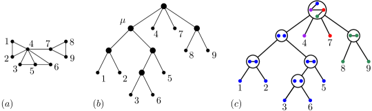
Figure 2: (a) A graph $G$. (b) The canonical modular decomposition of $G$ with $L(\mu)=\{1,2,3,5,6\}$. (c) The quotient graphs corresponding to the nodes in the canonical modular decomposition.

Observe that for any two nodes $\mu_{1},\mu_{2}\in T$ such that neither of them is an ancestor of the other, $G$ contains either all edges with one endpoint in $L(\mu_{1})$ and one endpoint in $L(\mu_{2})$ or none of them. For two vertices $u,v\in V$ we denote the lowest common ancestor of their corresponding leaves in $T$ by $\mathrm{lca}_{T}(u,v)$. For a set of leaves $L$, we denote the lowest common ancestor by $\mathrm{lca}_{T}(L)$.

With each inner node $\mu$ of $T$ we associate a quotient graph $G[\mu]$ that is obtained from $G[L(\mu)]$ by contracting $L(\nu)$ into a single vertex for each child $\nu$ of $\mu$; see Figure 2. In the rest of this paper we identify the vertices of $G[\mu]$ with the corresponding children of $\mu$. Every edge $uv\in E$ is represented by exactly one edge $\mathrm{rep}_{T}(uv)$ in one of the quotient graphs of $T$, namely in the quotient graph $G[\mu]$ of the lowest common ancestor $\mu$ of $u$ and $v$. More precisely, if $\nu$ and $\lambda$ are the children of $\mu$ with $u\in L(\nu)$ and $v\in L(\lambda)$, then $\mathrm{rep}_{T}(uv)$ $=$ $\nu\lambda$. For an oriented edge $uv$, $\mathrm{rep}_{T}(uv)$ is also oriented towards its endpoint $\nu$ with $v\in L(\nu)$. If $T$ is clear from the context, the subscript can be omitted. Let $\mu$ be a node in $T$. For a vertex $u\in L(\mu)$ we denote the child $\lambda$ of $\mu$ with $u\in L(\lambda)$ by $\text{rep}_{\mu}(u)$.

A node $\mu$ in a modular decomposition $T$ is called empty, complete or prime if the quotient graph $G[\mu]$ is empty, complete or prime, respectively. By $K(T)$, $P(T)$ we denote the set of all complete and prime nodes in $T$, respectively. For every graph $G$ there exists a uniquely defined modular decomposition, that we call the canonical modular decomposition of $G$, introduced by Gallai [17], such that each quotient graph is either prime, complete or empty and, additionally, no two adjacent nodes are both complete or are both empty; see Figure 2. Note that in the literature, these are referred to as modular decompositions, whereas we use that term for general modular decompositions. For a prime node $\mu$ in the canonical modular decomposition of $G$, for every child $\nu$ of $\mu$, $L(\nu)$ is a maximal module in $G[L(\mu)]$ and for every maximal module $M$ in $G[L(\mu)]$ there exists a child $\nu$ of $\mu$ with $L(\nu)=M$. McConnell and Spinrad showed that the canonical modular decomposition can be computed in $O(|V|+|E|)$ time [31]. Let $\mu$ be a node in a modular decomposition for $G$. A $\mu$-set $U$ is a subset of $L(\mu)$ that contains for each child $\lambda$ of $\mu$ at most one leaf in $L(\lambda)$. If $U$ contains for every child $\lambda$ of $\mu$ a vertex in $L(\lambda)$, we call it maximal.

Lemma 2.1.

Let $T$ be a modular decomposition of a graph $G$. After a linear-time preprocessing we can assume that each node of $T$ is annotated with its quotient graph. Moreover, the following queries can be answered in $O(1)$ time:

1. Given a non-root node $\nu$ of $T$, find the vertex of the quotient graph of $\nu$’s parent that corresponds to $\nu$.

2. Given a vertex $v$ in a quotient graph $G[\mu]$, find the child of $\mu$ that corresponds to $v$.

3. Given an edge $e$ of $G$, determine $\mathrm{rep}(e)$, the quotient graph that contains $\mathrm{rep}(e)$, and which endpoint of $\mathrm{rep}(e)$ corresponds to which endpoint of $e$.

Additionally, given a node $\mu$ in $T$ one can find a maximal $\mu$-set $U$ in $O(|U|)$ time.

Proof 2.2.

We focus on constructing the quotient graphs. The queries can be answered by suitably storing pointers during the construction. For every node $\mu$ in $T$ we initiate the quotient graph with one vertex for each child of $\mu$ and equip the children of $\mu$ and their corresponding vertices with pointers so that queries 1) and 2) can be answered in $O(1)$ time.

Next, we compute the edges of the quotient graphs. The difficulty here is to find for each edge $uv$ in a quotient graph $G[\mu]$ the children $\lambda_{u}$, $\lambda_{v}$ of $\mu$ with $u\in L(\lambda_{u})$ and $v\in L(\lambda_{v})$. For each node $\mu$ of $T$ we compute a list $L_{\mu}$ that contains all edges $uv$ of $G$ with $\operatorname{\mathrm{lca}}_{T}(u,v)=\mu$. Namely, we use the lowest-common-ancestor data structure for static trees of Harel and Tarjan [22], to compute $\operatorname{\mathrm{lca}}_{T}(u,v)$ for each edge $uv$ and add $uv$ to $L_{\operatorname{\mathrm{lca}}(u,v)}$. Afterwards, we perform a bottom-up traversal of the inner nodes of $T$ that maintains for each leaf $v$ of $T$ the processed root $r(v)=\mu$, where $\mu$ is the highest already-processed node of $T$ with $v\in L(\mu)$.

Initially, we set $r(v)=v$ for all leaves of $T$, and we mark all leaves as processed. When processing a node $\mu$, we determine the edges of $G[\mu]$ as follows. We traverse the list $L_{\mu}$ and for each edge $uv\in L_{\mu}$, we determine the children $r(u)$ and $r(v)$ of $\mu$. From this, we determine the corresponding vertices of $G[\mu]$ and add an edge with a pointer to $uv$ between them. This may create multi-edges. We find those by sorting the incidence list of each vertex by the number of the other incident node in linear time using radix sort [13] and an arbitrary enumeration of $V(G[\mu])$. We then replace all parallel edges between two vertices with a single edge and annotate it with all pointers of the merged edges. For each pointer from an edge $e$ in $G[\mu]$ to a represented edge $uv$, we then annotate $uv$ with a pointer to $e$.

Afterwards, we update $r(v)$ for all $v\in L(\mu)$ to $\mu$ and mark $\mu$ as processed. To maintain the processed roots of all leaves, we employ a union-find data structure, which initially contains one singleton set for each leaf and when a node $\mu$ has been processed, we equip it with a maximal $\mu$-set containing an arbitrarily chosen vertex from every set associated with a child of $\mu$ and afterwards unite the sets associated with its children. Since the union-find tree is known in advance (it corresponds to $T$), the union-find operations can be performed in amortized $\mathcal{O}(1)$ time [16].

We observe that the total size of all lists $L_{\mu}$ is $O(m)$ and moreover $T$ has at most $2n-1$ nodes. Therefore the whole preprocessing runs in linear time.

Let $\mu$ be a node in a modular decomposition $T$ of $G$ and let $\mu_{1}\mu_{2}$ be an edge in $G[\mu]$. Let $\vec{T}[G]$ denote an assignment of directions to all edges in $G[\mu]$ for every node $\mu$ in $T$. Such a $\vec{T}[G]$ is transitive if it is transitive on every $G[\mu]$. We obtain an orientation of $G$ from an orientation $\vec{T}[G]$ of the quotient graphs of $T$ as follows. Every undirected edge $uv$ in $E$ with $\mathrm{rep}(uv)$ $=\mu_{1}\mu_{2}\in\vec{T}[G]$, is directed from $u$ to $v$. We say that $T$ represents an orientation $O$ of $G$, if there exists an orientation $\vec{T}[G]$ of the quotient graphs of $T$ that gives us $O$. We denote the set of all transitive orientations of $G$ represented by $T$ by $\mathrm{to}(T)$. We get an orientation of the quotient graphs of $T$ from an orientation of $G$, if for each oriented edge $\mu_{1}\mu_{2}$, all edges represented by $\mu_{1}\mu_{2}$ are oriented from $L(\mu_{1})$ to $L(\mu_{2})$. Let $T$ now be the canonical modular decomposition of $G$. Then $T$ represents exactly the transitive orientations of $G$ [17]. It follows that $G$ is a comparability graph if and only if $T$ can be oriented transitively.

If $G$ is a comparability graph, every prime quotient graph $G[\mu]=(V_{\mu},E_{\mu})$ has exactly two transitive orientations, one the reverse of the other [20], and with the algorithm by McConnell and Spinrad [31] we can compute one of them in $O(|V_{\mu}|+|E_{\mu}|)$ time. Hence the time to compute the canonical modular decomposition in which every prime node is labeled with a corresponding transitive orientation is $O(|V|+|E|)$.

3 Transitive Orientation Extension

The partial orientation extension problem for comparability graphs OrientExt is to decide for a comparability graph $G$ with a partial orientation $W$, i.e. an orientation of some of its edges, whether there exists a transitive orientation $O$ of $G$ with $W\subseteq O$. The notion of partial orientations and extensions extends to modular decompositions. We get a partial orientation of the quotient graphs of $T$ from $W$ such that exactly the edges that represent at least one edge in $W$ are oriented and all edges in $W$ that are represented by the same oriented edge $\mu_{1}\mu_{2}$, are directed from $L(\mu_{1})$ to $L(\mu_{2})$.

Lemma 3.1.

Let $T$ be the canonical modular decomposition of a comparability graph $G$ and let $W$ be a partial orientation of $G$ that gives us a partial orientation $P$ of the quotient graphs of $T$. Then $W$ extends to a transitive orientation of $G$ if and only if $P$ extends to a transitive orientation of the quotient graphs of $T$.

Proof 3.2.

Let $O$ be a transitive orientation of $G$ that extends $W$. Let $\mu_{1}\mu_{2}$ be an oriented edge in $P$. Then $\mu_{1}\mu_{2}$ represents an oriented edge $uv$ in $W$. Then $uv$ is an oriented edge in $O$ and $\mu_{1}\mu_{2}$ is in the transitive orientation $\vec{T}[G]$ of the quotient graphs of $T$ we get from $O$. Hence, $\vec{T}[G]$ extends $P$.

Conversely, let $\vec{T}[G]$ be a transitive orientation of the quotient graphs of $T$ that extends $P$. Let $uv$ be an oriented edge in $W$. Then $uv$ is represented by an oriented edge $\mu_{1}\mu_{2}$ in $P$. Then $\mu_{1}\mu_{2}$ is an oriented edge in $\vec{T}[G]$ and $uv$ is in the transitive orientation $O$ of $G$ we get from $\vec{T}[G]$. Hence,$O$ extends $W$.

To solve OrientExt efficiently we confirm that the partial orientation actually gives us a partial orientation $P$ of the quotient graphs of the canonical modular decomposition $T$. Otherwise we can reject. By Lemma 3.1 we now just need to check for each node $\mu$ of $T$ whether $P$ can be extended to $G[\mu]$. To this end, we use that $\mu$ is empty, complete or prime. Since transitive orientations of cliques are total orders and prime graphs have at most two transitive orientations, the existence of an extension can easily be decided in each case.

Theorem 3.3.

OrientExt can be solved in linear time.

Proof 3.4.

Let $W$ be the given partial orientation of a comparability graph $G=(V,E)$. After the linear-time preprocessing of Lemma 2.1, we can compute the partial orientation $P$ of the quotient graphs of $T$ we get from $W$ in linear time by determining $\mathrm{rep}(uv)$ for every edge $uv\in W$. If $P$ does not exist, then there is an edge $\mu_{1}\mu_{2}$ in a quotient graph that represents an edge $e_{1}\in W$ oriented from $L(\mu_{1})$ to $L(\mu_{2})$ and an edge $e_{2}\in W$ oriented from $L(\mu_{2})$ to $L(\mu_{1})$. Then $W$ can not be extended to a transitive orientation of $G$ since in any orientation represented by $T$ the edges $e_{1}$, $e_{2}$ are both oriented in the same direction between $L(\mu_{1})$ and $L(\mu_{2})$. Hence, we can reject in this case.

Otherwise, to solve OrientExt for $G$, it suffices to solve OrientExt for every quotient graph in the canonical modular decomposition $T$ of $G$ with the partial orientation from $P$ by Lemma 3.1. Let $\mu$ be a node in $T$. We distinguish cases based on the type of $\mu$. If $\mu$ is empty, nothing needs to be done. If $\mu$ is complete, the problem of extending the partial orientation of $G[\mu]$ is equivalent to the problem of finding a total order of the nodes of $G[\mu]$ that respects $P$. This can be done via topological sorting in linear time. If $\mu$ is prime, $G[\mu]$ has exactly two transitive orientations, where one is the reverse of the other. Therefore we check in linear time whether one of these orientations of $G[\mu]$ is an extension of the partial orientation of $G[\mu]$. Otherwise, no transitive extension exists.

Since we can compute $T$ in $O(|V|+|E|)$ time, in total we can decide whether the partial orientation $W$ is extendible in the same time. we get a corresponding transitive orientation of $G$ by the extension of $P$ and can also be computed in the same time.

4 Sunflower Orientations

The idea to solve SimOrient^⋆ is to obtain for each input graph $G_{i}$ a restricted modular decomposition of the shared graph $H$ that represents exactly those transitive orientations of $H$ that can be extended to $G_{i}$. The restricted modular decompositions can be expressed by constraints for the canonical modular decomposition of $H$. These constraints are then combined to represent all transitive orientations of $H$ that can be extended to each input graph $G_{i}$. With this the solution is straightforward.

Let $H$ be a comparability graph. Then we define a restricted modular decomposition $(T,D)$ of $H$ to be a tuple where $T$ is a modular decomposition of $H$ where every node is labeled as complete, empty or prime, such that for every node $\mu$ labeled as complete or empty, $H[\mu]$ is complete or empty, respectively, and $D$ is a function that assigns to each prime labeled node $\mu$ a transitive orientation $D_{\mu}$, called default orientation. In the following, when referring to the type of a node $\mu$ in a restricted modular decomposition, we mean the type that $\mu$ is labeled with. A transitive orientation of $(T,D)$, is a transitive orientation of the quotient graphs of $T$ where every prime node $\mu$ has orientation $D_{\mu}$ or its reversal $D_{\mu}^{-1}$. Let $\mathrm{to}(T,D)$ denote the set of transitive orientations of $H$ we get from transitive orientations of $(T,D)$. We say $(T,D)$ represents these transitive orientations. Note that for the canonical modular decomposition $B$ of $H$ we have $\mathrm{to}(T,D)\subseteq\mathrm{to}(B)$.

Let $G$ be a comparability graph with an induced subgraph $H$. A modular decomposition $T$ of $G$ gives us a restricted modular decomposition $(T|_{H},D)$ of $H$ as follows; see Figure 3.

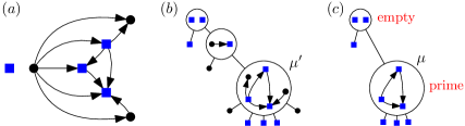
Figure 3: (a) A graph $G$ with an induced subgraph $H$ (blue square vertices). (b) A modular decomposition $T$ of $G$ with a transitive orientation. (c) The restricted modular decomposition $(T|_{H},D)$ of $H$ derived from the transitive orientation in (b). Note that $H[\mu]$ is a clique but $\mu$ is labeled prime.

We obtain $T|_{H}$ from $T$ by (i) removing all leaves that do not correspond to a vertex of $H$ and then (ii) iteratively contracting all inner nodes of degree at most 2. With a bottom-up traversal we can compute $T|_{H}$ in time linear in the size of $T$. A node $\mu$ in $T|_{H}$ stems from $\operatorname{\mathrm{lca}}_{T}(L(\mu))$. Every node $\mu\in T|_{H}$ that stems from a prime node $\mu^{\prime}\in T$ we label as prime and set $D_{\mu}$ to a transitive orientation of $G[\mu^{\prime}]$ restricted to the edges of $H$. The remaining nodes are labeled according to the type of their quotient graph. Note that $H[\mu]$ is isomorphic to an induced subgraph of $G[\mu^{\prime}]$.

Lemma 4.1.

Let $T$ be a modular decomposition of a graph $G$ with an induced subgraph $H$. Then $\mathrm{to}(T|_{H},D)$ is the set of orientations of $H$ extendable to transitive orientations of $G$.

Proof 4.2.

Let $O_{H}$ be a transitive orientation of $H$ that can be extended to a transitive orientation $O_{G}$ of $G$. Then $O_{G}$ gives us a transitive orientation $\vec{T}[G]$ of the quotient graphs of $T$ that in turn gives us a transitive orientation $\vec{T}|_{H}$ of $(T|_{H},D)$. Since $O_{G}$ is an extension of $O_{H}$ and $\vec{T}[G]$ contains $\vec{T}_{H}[H]$, $O_{H}$ is the transitive orientation of $H$ we get from $\vec{T}_{H}[H]$. Hence $(T|_{H},D)$ represents $O_{H}$.

Conversely, let $\vec{T}_{H}[H]$ be a transitive orientation of $(T_{H},D)$. For any node $\mu$ in $T|_{H}$ let $\mu^{\prime}=\mathrm{lca}_{T}(L(\mu))$. Recall that $H[\mu]$ is isomorphic to an induced subgraph of $G[\mu^{\prime}]$. We already know that $G[\mu^{\prime}]$ is either empty, complete or prime. If $G[\mu^{\prime}]$ is empty, $H[\mu]$ and the corresponding transitive orientation are also empty. If $G[\mu^{\prime}]$ is complete, then $H[\mu]$ is also complete and any transitive orientation of $H[\mu]$ can be extended to a transitive orientation of $G[\mu^{\prime}]$. If $G[\mu^{\prime}]$ is prime, by construction $H[\mu]$ is also labeled as prime with a default orientation $D_{\mu}$ given by a transitive orientation $D_{\mu^{\prime}}$ of $G[\mu^{\prime}]$. Hence $\vec{T}_{H}[H]$ either contains $D_{\mu^{\prime}}\cap E(H[\mu])=D_{\mu}$ or $D_{\mu^{\prime}}^{-1}\cap E(H[\mu])=D_{\mu}^{-1}$. Thus $\vec{T}_{H}[H]$ can be mapped to $T$ and be extended to a transitive orientation $\vec{T}[G]$ of the quotient graphs of $T$. Then $\vec{T}[G]$ gives us a transitive orientation $O_{G}$ of $G$ since $T$ represents exactly the transitive orientations of $G$. Let $O_{H}$ be $O_{G}$ restricted to $H$. Then by construction $O_{H}$ equals the orientation of $H$ we get from $\vec{T}_{H}[H]$. Thus $\vec{T}_{H}[H]$ gives us a transitive orientation of $H$.

Consider the canonical modular decompositions $T^{1},\dots,T^{r}$ of the input graphs $G_{1},\dots,G_{r}$, and let $(T^{1}|_{H},D_{1}),\dots,(T^{r}|_{H},D_{r})$ be the corresponding restricted modular decompositions. Then we are interested in the intersection $\mathrm{to}(G_{1},\dots,G_{r})=\bigcap_{i=1}^{r}\mathrm{to}(T^{i}|_{H},D_{i})$ since it contains all transitive orientations of $H$ that can be extended to all input graphs. However, the trees $T^{1}|_{H},\dots,T^{r}|_{H}$ have different shapes, which makes it difficult to compute a representation of $\mathrm{to}(G_{1},\dots,G_{r})$ directly. Instead, we describe $\mathrm{to}(T^{1}|_{H},D_{1}),\dots,\mathrm{to}(T^{r}|_{H},D_{r})$ (whose intersection is simple to compute) with constraints on the canonical modular decomposition $B$ of $H$.

Let $(T,D)$ be a restricted modular decomposition of $H$ and let $B$ be the canonical modular decomposition of $H$. We collect constraints on the orientations of individual nodes $\mu$ of $B$ that are imposed by $\mathrm{to}(T,D)$. Afterwards we show that the established constraints are sufficient to describe $\mathrm{to}(T,D)$. If $\mu$ is empty, then $H[\mu]$ is empty and has a unique transitive orientation, which requires no constraints. The other types of $\mu$ are discussed in the following two sections.

4.1 Constraints for Prime Nodes

In this section we observe that prime nodes in $B$ correspond to prime nodes in $(T,D)$ and that the dependencies between their orientations can be described with 2-SAT formulas. Recall that the transitive orientation of a prime comparability graph is unique up to reversal. We consider each prime node $\mu\in B$ equipped with a transitive orientation $D_{\mu}$, also called a default orientation. All default orientations for $B$ can be computed in linear time [31].

Lemma 4.3.

Let $\mu\in B$ be prime. Then $\mu^{\prime}=\operatorname{\mathrm{lca}}_{T}(L(\mu))$ is prime, every $\mu$-set is a $\mu^{\prime}$-set, and for any edge $uv$ with $\mathrm{rep}_{B}(uv)\in H[\mu]$ we have $\mathrm{rep}_{T}(uv)\in H[\mu^{\prime}]$.

Proof 4.4.

We first show that every $\mu$-set is also a $\mu^{\prime}$-set. Assume there is a $\mu$-set $U$ that is not a $\mu^{\prime}$-set. Since $U\subseteq L(\mu)\subseteq L(\mu^{\prime})$, there exist two vertices $u\neq v\in U$ with $\lambda=\text{rep}_{\mu^{\prime}}(u)=\text{rep}_{\mu^{\prime}}(v)$. From $L(\lambda)$ being a module of $H[L(\mu^{\prime})]$ and $L(\mu)\subseteq L(\mu^{\prime})$ it follows that $X=L(\lambda)\cap L(\mu)$ is a module of $H[L(\mu)]$. By the definition of $\mu^{\prime}$, we have  $X\subsetneq L(\mu)$. Since $\mu$ is prime, there is a child $\nu$ of $\mu$ with $u,v\in X\subseteq L(\nu)$ contradicting $U$ being a $\mu$-set.

As a direct consequence of $\mu$-sets being $\mu^{\prime}$-sets, we also have for any edge $uv$ with $\mathrm{rep}_{B}(uv)\in H[\mu]$ that $\mathrm{rep}_{T}(uv)\in H[\mu^{\prime}]$ since $\{u,v\}$ is a $\mu$-set. Now let $U$ be a maximal $\mu$-set. Then $H[U]$ is isomorphic to $H[\mu]$ and thus prime. Since $U$ is also a $\mu^{\prime}$-set and the subgraph of $H[\mu^{\prime}]$ induced by the vertices representing $U$ is isomorphic to $H[U]$, $\mu^{\prime}$ is neither empty, nor complete and thus prime.

For a modular decomposition $T^{\prime}$ of $H$ with a node $\lambda$ and $O\in\mathrm{to}(T^{\prime})$ let $O_{\downarrow\lambda}$ denote the orientation of the quotient graph $H[\lambda]$ we get from $O$. Note that for a transitive orientation $D_{\lambda}$ of $H[\lambda]$ and a $\lambda$-set $U$ each orientation $O\in\mathrm{to}(T^{\prime})$ with $O_{\downarrow\lambda}=D_{\lambda}$ gives us the same orientation on $H[U]$. We say that $D_{\lambda}$ induces this orientation on $H[U]$.

Let $\mu\in B$ be prime, let $\mu^{\prime}=\operatorname{\mathrm{lca}}_{T}(L(\mu))$ and let $U$ be a maximal $\mu$-set (and by Lemma 4.3 a $\mu^{\prime}$-set). We set $D^{\delta}_{\mu^{\prime}}=D_{\mu^{\prime}}$ if $D_{\mu}$, $D_{\mu^{\prime}}$ induce the same transitive orientation on the prime graph $H[U]$ and we set $D^{\delta}_{\mu^{\prime}}=D^{-1}_{\mu^{\prime}}$ if the induced orientations are the reversal of each other. Note that $D^{\delta}_{\mu^{\prime}}$ does not depend on the choice of $U$. From the definition of $D^{\delta}_{\mu^{\prime}}$ and the observation that $O_{\downarrow\mu},O_{\downarrow\mu^{\prime}}$ are both determined by $O$ restricted to $H[U]$ we directly get the following lemma.

Lemma 4.5.

For $O\in\mathrm{to}(T,D)$ we have $O_{\downarrow\mu}=D_{\mu}\Leftrightarrow O_{\downarrow\mu^{\prime}}=D^{\delta}_{\mu^{\prime}}$

We express the choice of a transitive orientation for a prime node $\mu$ by a Boolean variable $x_{\mu}$ that is $\mathtt{true}$ for the default orientation and $\mathtt{false}$ for the reversed orientation.

According to Lemma 4.5 we set $\psi_{\mu}$ to be $x_{\mu}\leftrightarrow x_{\mu^{\prime}}$ if $D_{\mu^{\prime}}^{\delta}=D_{\mu^{\prime}}$ and $x_{\mu}\not\leftrightarrow x_{\mu^{\prime}}$ if $D_{\mu^{\prime}}^{\delta}=D^{-1}_{\mu^{\prime}}$. Note that for a prime node $\mu^{\prime}\in T$ there may exist more than one prime node $\mu$ in $B$ such that $\mu^{\prime}=\mathrm{lca}_{T}(L(\mu))$, and we may hence have multiple prime nodes that are synchronized by these constraints. We describe these dependencies with the formula $\psi=\bigwedge_{\mu\in P(B)}\psi_{\mu}$. With the above meaning of variables, any choice of orientations for the prime nodes of $B$ that can be induced by $T$ necessarily satisfies $\psi$. With Lemma 2.1 we can compute $\psi$ efficiently.

Lemma 4.6.

We can compute $\psi$ in $O(|V(H)|+|E(H)|)$ time.

Proof 4.7.

Let $\mu$ be a prime node in $B$ and let $\mu^{\prime}=\mathrm{lca}_{T}(L(\mu))$. By Lemma 2.1 we can compute a maximal $\mu$-set $U$ in constant time after a linear-time preprocessing. By Lemma 4.3 we have for every edge $uv$ with $\mathrm{rep}_{B}(uv)\in H[\mu]$ that $\mathrm{rep}_{T}(uv)\in H[\mu^{\prime}]$. Hence we can find $\mu^{\prime}$ in $T$ by determining $\mathrm{rep}_{T}(uv)$ for an arbitrary edge $uv$ with  $u,v\in U$, which by Lemma 2.1 takes constant time. For an arbitrary oriented edge $e\in O$ we check in constant time whether $e\in D_{\mu}$ or $e\in D_{\mu}^{-1}$ and add the clause $x_{\mu}\leftrightarrow x_{\mu^{\prime}}$ or $x_{\mu}\not\leftrightarrow x_{\mu^{\prime}}$, respectively. Doing this for every prime node in total takes time linear in the size of $T$.

4.2 Constraints for Complete Nodes

Next we consider the case where $\mu$ is complete. The edges represented in $H[\mu]$ may be represented by edges in more than one quotient graph in $T$, each of which can be complete or prime. Depending on the type of the involved quotient graphs in $T$ we get new constraints for the orientation of $H[\mu]$.

Note that choosing a transitive orientation of $H[\mu]$ is equivalent to choosing a linear order of the vertices of $H[\mu]$. As we will see, each node $\nu$ of $T$ that represents an edge of $H[\mu]$ imposes a consecutivity constraint on a subset of the vertices of $H[\mu]$. Therefore, the possible orders can be represented by a PQ-tree that allows us to represent all permissible permutations of the elements of a set $U$ in which certain subsets $S\subseteq U$ appear consecutively.

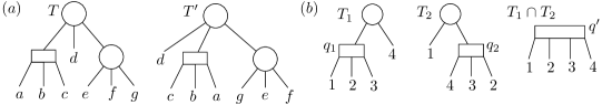
Figure 4: (a) Two equivalent PQ-trees $T$, $T^{\prime}$ with $fr(T)=abcdefg$ and $fr(T^{\prime})=dcbagef$. (b) The Q-node $q^{\prime}$ in $T_{1}\cap T_{2}$ contains $q_{1}$ forwards and $q_{2}$ backwards.

PQ-trees were first introduced by Booth and Lueker [7, 8]. A PQ-tree $T$ over a finite set $U$ is a rooted tree whose leaves are the elements of $U$ and whose internal nodes are labeled as $P$- or $Q$-nodes. A $P$-node is depicted as a circle, a $Q$-node as a rectangle; see Figure 4. Two PQ-trees $T$ and $T^{\prime}$ are equivalent, if $T$ can be transformed into $T^{\prime}$ by arbitrarily permuting the children of arbitrarily many $P$-nodes and reversing the order of arbitrarily many $Q$-nodes; see Figure 4a. A transformation that transforms $T$ into an equivalent tree $T^{\prime}$ is called an equivalence transformation. The frontier $\operatorname{\mathrm{fr}}(T)$ of a PQ-tree $T$ is the order of its leaves from left to right. The tree $T$ represents the frontiers of all equivalent $PQ$-trees. The PQ-tree that does not have any nodes is called the null tree.

Let $T_{1}$, $T_{2}$ be two PQ-trees over a set $U$. Their intersection $T=T_{1}\cap T_{2}$ is a PQ-tree that represents exactly the linear orders of $U$ represented by both $T_{1}$ and $T_{2}$. It can be computed in $O(|U|)$ time [7]. For every Q-node $q$ in $T_{1}$ node $q^{\prime}=\operatorname{\mathrm{lca}}_{T}(L(q))$ is also a Q-node. We say that $q^{\prime}$ contains $q$ forwards, if $T_{1}[q]$ can be transformed by an equivalence transformation that does not reverse $q$ into a PQ-tree $T^{\prime}$ such that $\operatorname{\mathrm{fr}}(T[q])$ contains $\operatorname{\mathrm{fr}}(T[q^{\prime}])$; see Figure 4b. Else $q^{\prime}$ contains $q$ backwards. Similarly every Q-node in $T_{2}$ is contained in exactly one Q-node in $T$ (either forwards or backwards). Haeupler et al. [21] showed that one can modify Booth’s algorithm such that given two PQ-trees $T_{1},T_{2}$ it not only outputs  $T_{1}\cap T_{2}$ but also for every Q-node in $T_{1},T_{2}$ which Q-node in $T$ contains it and in which direction.

Lemma 4.8.

Let $T_{1},\dots,T_{k}$ be PQ-trees over a set $U$. Then we can compute their intersection $T=\bigcap_{i=1}^{k}T_{i}$ and determine for every Q-node $q$ in $T_{1},\dots,T_{k}$ the Q-node in $T$ that contains $q$ and in which direction in $O(k\cdot|U|)$ time.

Proof 4.9.

Let $S_{1}=T_{1}$ and for every $j\in\{2,\dots,k\}$ let  $S_{j}:=S_{j-1}\cap T_{i}$. To compute $T=S_{k}$ we stepwise compute $S_{j}=S_{j-1}\cap T_{j}$ for every $j$. During the computation of $T$ we construct a DAG $D$ whose vertices are the Q-nodes of $T_{1},\dots,T_{k}$ and $S_{2},\dots,S_{k}$. Initially $D$ contains no edges. For every $j$ we add a directed edge from every Q-node $q$ in $T_{j}$ and $S_{j-1}$ to the Q-node $q^{\prime}$ in $S_{j}$ that contains $q$. We label the edge with 1 if $q^{\prime}$ contains $q$ forwards, and with -1 otherwise. By the result of Haeupler et al. this can be done in $O(k\cdot|U|)$ time [21]. Note that by construction every vertex has at most one outgoing edge and for every Q-node $q$ in $T_{1},\dots,T_{k}$ there is a unique path to the Q-node $q^{\prime}$ in $S_{k}$ that contains it. The product of the edge labels along this path is 1 and -1 if $q^{\prime}$ contains $q$ forwards and backwards, respectively.

To determine for every Q-node $q$ in $T_{1},\dots,T_{k}$ which Q-node in $T$ contains it and in which direction, we start at the sinks in $D$ and backward propagate for every vertex in $D$ the information which unique sink $q^{\prime}$ can be reached from it and what is the product of edge labels along the path to $q^{\prime}$. This needs $O(k\cdot|U|)$ time since the $D$ has $O(k\cdot|U|)$ vertices and edges.

Let $\mu^{\prime}=\mathrm{lca}_{T}(L(\mu))$ for the rest of this section

Figure 5: (a) A graph $H$. (b) The canonical modular decomposition $B$ of $H$. (c) A restricted modular decompositions $T$ of $H$. (d) The PQ-tree $S_{\mu}$. The active nodes of $T$ with regard to the $\mu$-set $\{2,4,6\}$ are $\nu_{1}^{\prime}$, $\nu_{2}^{\prime}$, 2, 4 and 6.

and let $U\subseteq V$ be a maximal $\mu$-set. We call a node of $T$ active if it is either a leaf in $U$ or if at least two of its subtrees contain leaves in $U$. Denote by $A$ the set of active nodes in $T$ and observe that $A$ can be turned into a tree $S_{\mu}$ by connecting each node $\nu^{\prime}\in A\setminus\{\mu^{\prime}\}$ to its lowest active ancestor; see Figure 5. Let now $\vec{B}[H]$ be an orientation of the quotient graphs of  $B$ induced by an orientation $\vec{T}[G]\in\mathrm{to}(T,D)$ and consider a node $\nu^{\prime}\neq\mu^{\prime}$ of $S_{\mu}$. Let $X=U\cap L(\nu^{\prime})$ and let $Y=U\setminus L(\nu^{\prime})$. Since $U$ is a $\mu$-set of a complete node, any pair of vertices in $X\times Y$ is adjacent. Moreover, for each $y\in Y$, the edges from $y$ to $X$ are all oriented towards $X$, or they are all oriented towards $y$, since every node of $T$ that determines the orientation of such an edge contains all vertices of $X$ in a single child. This implies that in the order of the $\mu$-set given by the order of $H[\mu]$, the set $L(\nu^{\prime})$ is consecutive. Moreover, if $\nu^{\prime}$ is prime, its default orientation $D_{\nu^{\prime}}$ induces a total order on the active children of $\nu^{\prime}$ that is fixed up to reversal. Hence we turn $S_{\mu}$ into a PQ-tree by first turning all complete nodes into P-nodes and all prime nodes into Q-nodes with the children ordered according to the linear order determined by the default orientation which we call the initial order of the Q-node. Finally, we replace each leaf $v\in U$ by the corresponding vertex $\mathrm{rep}_{\mu}(v)$ of $H[\mu]$; see Figure 5. As argued above, the linear order of $H[\mu]$ is necessarily represented by $S_{\mu}$.

We show that tree $S_{\mu}$ is independent from the choice of the maximal $\mu$-set $U$. We use that any node of $T$ has a laminar relation to the children of $\mu$.

Lemma 4.10.

For any child $\mu_{1}$ of $\mu$ and any node $\kappa^{\prime}$ of $V(T)$ we have $L(\mu_{1})\subseteq L(\kappa^{\prime})\cap L(\mu)$ or $L(\kappa^{\prime})\cap L(\mu)\subseteq L(\mu_{1})$.

Figure 6: (a) A subtree of $B$ with root $\mu$. (b) A subtree of $T$ with root $\nu^{\prime}$.

Proof 4.11.

If $L(\kappa^{\prime})$ contains only leaves of at most one child $\mu_{1}$ of $\mu$, we have $L(\kappa^{\prime})\cap L(\mu)\subseteq L(\mu_{1})$ and $L(\mu_{2})\subseteq L(\kappa^{\prime})\cap L(\mu)$ for each other child $\mu_{2}$ of $\mu$. Otherwise, let $\mu_{1}$, $\mu_{2}$ be children of $\mu$ with leaves $u\in L(\kappa^{\prime})\cap L(\mu_{1})$, $v\in L(\kappa^{\prime})\cap L(\mu_{2})$ and let $\lambda^{\prime}=\mathrm{lca}_{T}(u,v)$; see Figure 6. Note that $\lambda^{\prime}$ is a descendant of $\kappa^{\prime}$ or $\lambda^{\prime}=\kappa^{\prime}$. Assume that there exists a vertex $w\in L(\mu_{1})\setminus L(\kappa^{\prime})$ and let $\nu^{\prime}=\mathrm{lca}_{T}(u,w)$. Then $\kappa^{\prime}$ is a descendant of $\nu^{\prime}$ since $u\in L(\nu^{\prime})\cap L(\kappa^{\prime})$ and $w\in L(\nu^{\prime})\setminus L(\kappa^{\prime})$. Note that $\mathrm{rep}_{T}(vw)=\mathrm{rep}_{T}(uw)\in H[\nu^{\prime}]$ and $\mathrm{rep}_{T}(uv)\in H[\lambda^{\prime}]$. Hence, $T$ represents a transitive orientation of $H$ with $uv$ and $vw$. This contradicts $B$ representing all transitive orientations of $H$ since we have $\mathrm{rep}_{B}(uv)=\mathrm{rep}_{B}(wv)$. It follows that $L(\mu_{1})\setminus L(\kappa^{\prime})=\emptyset$ and analogously $L(\mu_{2})\setminus L(\kappa^{\prime})=\emptyset$. This concludes the proof.

Lemma 4.12.

Let $S_{\mu}^{1}$, $S_{\mu}^{2}$ be the PQ-trees for two maximal $\mu$-sets $U_{1}$, $U_{2}$. Then $S_{\mu}^{1}=S_{\mu}^{2}$.

Proof 4.13.

Let $\nu^{\prime}$ be a non-leaf node in $T$ that is active with regard to $V_{1}^{\prime}$. Then there exist two vertices $u_{1},v_{1}\in V_{1}^{\prime}$ and two distinct children $\nu_{1}^{\prime}$, $\nu_{2}^{\prime}$ of $\nu^{\prime}$ such that $u_{1}\in L(\nu_{1}^{\prime})$ and $v_{1}\in L(\nu_{2}^{\prime})$. Let $\mu_{1}=\mathrm{rep}_{\mu}(u_{1})$, $\mu_{2}=\mathrm{rep}_{\mu}(v_{1})$ and let $u_{2}$, $v_{2}$ be the vertices in $V_{2}^{\prime}$ with $\mathrm{rep}_{\mu}(u_{2})=\mu_{1}$, $\mathrm{rep}_{\mu}(v_{2})=\mu_{2}$. We prove the following:

1. $u_{2},v_{2}\in L(\nu^{\prime})$

2. $\mathrm{rep}_{\nu^{\prime}}(u_{2})\neq\mathrm{rep}_{\nu^{\prime}}(v_{2})$

3. $\mathrm{rep}_{\nu^{\prime}}(u_{1}v_{1})\in D_{\nu^{\prime}}\Leftrightarrow\mathrm{rep}_{\nu^{\prime}}(u_{2}v_{2})\in D_{\nu^{\prime}}$.

For Statement i we get $u_{2}\in L(\mu_{1})\subseteq L(\nu^{\prime})\cap L(\mu)$ by Lemma 4.10 since $v_{1}\not\in L(\mu_{1})$ and similarly $v_{2}\in L(\nu^{\prime})\cap L(\mu)$.

For Statement ii assume $\nu^{\prime\prime}=\mathrm{rep}_{\nu^{\prime}}(u_{2})=\mathrm{rep}_{\nu^{\prime}}(v_{2})$. Then we have $u_{2}\in L(\nu^{\prime\prime})$ and $u_{2}\not\in L(\mu_{1})$. By Lemma 4.10 we get $u_{1}\in L(\mu_{1})\subseteq L(\nu^{\prime\prime})\cap L(\mu)$, i.e., $\nu^{\prime\prime}=\nu^{\prime}_{1}$ and similarly $\nu^{\prime\prime}=\nu^{\prime}_{2}$ in contradiction to $\nu^{\prime}_{1}\neq\nu^{\prime}_{2}$.

For Statement iii note that $u_{1}v_{1}$ and $u_{2}v_{2}$ are indeed represented in $\nu^{\prime}$ by Statement ii and they are both represented by $\mu_{1}\mu_{2}$ in $H[\mu]$.

It follows that the active inner nodes are the same for $U_{1}$, $U_{2}$ and after replacing the leaves with the children of $\mu$ we obtain the same trees. Statement iii then provides that the ordering of the children of $Q$-nodes is also the same and $S_{\mu}^{1}$, $S_{\mu}^{2}$ are indeed the same PQ-tree.

By construction, each Q-node $q$ of $S_{\mu}$ stems from a prime node $\nu^{\prime}$ in $T$, and the orientation of $T[\nu^{\prime}]$ determines the orientation of $q$, namely $q$ is reversed if and only if $T[\nu^{\prime}]$ is oriented as $D_{\nu^{\prime}}^{-1}$. Since a single prime node $\nu^{\prime}$ of $T$ may give rise to Q-nodes in several PQ-trees $S_{\mu}$, we need to ensure that the orientations of these Q-nodes are either all consistent with the default orientation of $T[\nu^{\prime}]$ or they are all consistent with its reversal. To model this, we introduce a Boolean variable $x_{q}$ for each Q-node $q$ in one of the PQ-trees with the interpretation that $x_{q}=\mathtt{true}$ if and only if $q$ has its initial order. We require $x_{q}$ to be equal to the variable that orients the prime node corresponding to $q$. More precisely, for every prime node $\nu^{\prime}$ in $T[\mu^{\prime}]$ that gives rise to $q$ we add the constraint $(x_{\nu^{\prime}}\leftrightarrow x_{q})$ to $\chi_{\mu}$, where the variable $x_{\nu^{\prime}}$ is the variable that encodes the orientation of the prime node $\nu^{\prime}$. We construct a Boolean formula by setting $\chi=\bigwedge_{\mu\in K(B)}\chi_{\mu}$.

Lemma 4.14.

We can compute all PQ-trees $S_{\mu}$ and the formula $\chi$ in $O(n+m)$ time.

Proof 4.15.

As a preprocessing we run a DFS on $T$ starting at the root and store for every node $\nu$ its discovery-time $\nu.d$, i.e., the timestamp when $\nu$ is first discovered, and its finish-time $\nu.f$, i.e., the timestamp after all its neighbors have been examined. We also employ the preprocessing from Lemma 2.1. We construct all PQ-trees and $\chi$ with the following steps.

1. Take a maximal $\mu$-set $U_{\mu}$ for every $\mu\in K(B)$.

2. For every $\mu\in K(B)$ compute the set of active nodes and for every active node compute its parent in $S_{\mu}$.

3. For every $\mu\in K(B)$ determine for each inner node of $S_{\mu}$ whether it is a P- or a Q-node. If it is a Q-node, determine the linear order of its children, and construct the formula $\chi_{\mu}$.

Step 1 can be done in $O(n)$ time by Lemma 2.1.

For Step 2, note that each active node is a least common ancestor of two leaves in $U_{\mu}$. While it is easy to get all active nodes as least common ancestors, getting the edges of $S_{\mu}$ requires more work. Observe that the DFS on $T$ visits the nodes of $S_{\mu}$ in the same order as a DFS on $S_{\mu}$. Consider $S_{\mu}$ embedded such that the children of each node are ordered from left to right by their discovery-times. This also orders the leaves from left to right by their discovery-times. Let $\lambda$ be an inner node of $S_{\mu}$. Let $\lambda_{1}$, $\lambda_{2}$ be two neighboring children of $\lambda$ with $\lambda_{1}$ to the left of $\lambda_{2}$. Then $\lambda$ is the least common ancestor of the rightmost leaf in $L(\lambda_{1})$ and the leftmost leaf in $L(\lambda_{2})$. Hence, each node of $S_{\mu}$ is a least common ancestor for a consecutive pair of leaves.

We add for every node $u$ in a set $U_{\mu}$ a tuple $(\mu,u.d)$ to an initially empty list $L$. We then sort the tuples in $L$ in linear time using radix sort [13]. In the sorted list, for every $\mu\in K(B)$ all tuples $(\mu,u.d)$ are consecutive and the consecutive sublist is sorted by discovery time.

For $\mu\in K(B)$ let $L_{\mu}$ be a list containing the vertices in $U_{\mu}$ ordered by their discovery time which we get directly from the consecutive sublist of $L$ containing the tuples corresponding to $\mu$. For every pair $u,v\in U_{\mu}$ adjacent in $L_{\mu}$ we compute $\lambda=\operatorname{\mathrm{lca}}_{T}(u,v)$ using the lowest-common-ancestor data structure for static trees by Harel and Tarjan [22] and insert $\lambda$ into $L_{\mu}$ between $u$ and $v$. For a vertex $u\in U_{\mu}$ its parent in $S_{\mu}$ is the neighbor in $L_{\mu}$ that has a lower position in $T$. Note that $u$ is a descendent in $T$ of all its neighbors in $L_{\mu}$. Hence if $u$ has two neighbors in $L_{\mu}$ one of them is a descendent of the other. Thus the parent of $u$ in $S_{\mu}$ is the neighbor with the higher discovery time. Now we remove all vertices in $U_{\mu}$ and possible duplicates of the remaining nodes from $L_{\mu}$. Note that still every $\lambda$ is a descendent in $T$ of its neighbors in $L_{\mu}$. Hence we iteratively choose a node $\lambda$ in $L_{\mu}$ whose discovery time is higher than the discovery time of its neighbors, compute its parent in $S_{\mu}$ by comparing the discovery times of its neighbors with each other and remove $\lambda$ from $L_{\mu}$.

In Step 3, we turn each active node that stems from a complete node into a P-node and each active node that stems from a prime node into a Q-node. For a Q-node $q$ that stems from a prime node $\nu$, we determine the linear order of its children as follows. Take the set $X$ of vertices of $H[\nu]$ that correspond to children of $\mu$ in $S_{\mu}$, determine the orientation of the complete graph on $X$ induced by $D_{\nu}$ and sort it topologically. In total this take $O(n+m)$ time for all active nodes in all PQ-trees. Using the information computed up to this point, it is straightforward to output the formula $\chi$.

Finally, we combine the constraints from the complete nodes with the constraints from the prime nodes by setting $\varphi_{T}=\psi\land\chi$. The formula $\varphi_{T}$ allows us to describe a restricted set of transitive orientations of $G$. We define $S_{T}=\{S_{\mu}\mid\mu\in K(B)\}$. The canonical modular decomposition $(B,S_{T},\varphi_{T})$ of $H$ where every complete node is labeled with the corresponding PQ-tree together with $\varphi_{T}$ we call a constrained modular decomposition.

We say that a transitive orientation $O$ of $H$ induces a variable assignment satisfying $\varphi_{T}$ if it induces an assignments of the variables corresponding to prime nodes in $B$ and $Q$-nodes such that $\varphi_{T}$ is satisfied for an appropriate assignment for the variables corresponding to prime nodes in $T$. Let $\mathrm{to}(B,S_{T},\varphi_{T})$ denote the set containing all transitive orientations $O\in\mathrm{to}(B)$ where for every complete node $\mu\in B$ the order $O_{\downarrow\mu}$ corresponds to a total order represented by $S_{\mu}$ and that induces a variable assignment that satisfies $\varphi_{T}$.

4.3 Correctness

We now show that $\mathrm{to}(B,S_{T},\varphi_{T})=\mathrm{to}(T,D)$. To this end we use that Lemma 4.3 allows to find for an edge $uv$ that is represented in a prime node $\mu$ of $B$ the prime node $\mu^{\prime}=\operatorname{\mathrm{lca}}_{T}(L(\mu))$ of $T$ where it is represented. This allows us to establish the identity of certain nodes. The following lemma does something similar for complete nodes.

Lemma 4.16.

Let $uv$, $wx$ be edges of $H$ represented in complete nodes $\mu$, $\nu$ of $B$ and by the same edge in a complete node of $T$. Then $\mu=\nu$.

Proof 4.17.

Let $\omega^{\prime}$ be the node in $T$ with $\mathrm{rep}_{T}(uv)\in H[\omega^{\prime}]$. Assume $\mu\neq\nu$. Then one of them is the ancestor of the other or they are both distinct from $\lambda=\mathrm{lca}_{B}(\mu,\nu)$. First consider the case that $\mu$ is an ancestor of $\nu$. Then $\mu$ has a child $\mu_{1}$ such that $L(\nu)\subseteq L(\mu_{1})$. Note that $\mathrm{rep}_{\mu}(u)\neq\mathrm{rep}_{\mu}(v)$, hence we have $\mathrm{rep}_{\mu}(u)\neq\mu_{1}$ or $\mathrm{rep}_{\mu}(v)\neq\mu_{1}$. Without loss of generality assume $\mathrm{rep}_{\mu}(u)\neq\mu_{1}$. Since $u\in L(\omega^{\prime})\cap L(\mu)\setminus L(\mu_{1})$ we have $L(\mu_{1})\subseteq L(\omega^{\prime})$ by Lemma 4.10 and analogously it follows that $L(\mathrm{rep}_{\mu}(u))\subseteq L(\omega^{\prime})$. Since $\mathrm{rep}_{T}(wx)=\mathrm{rep}_{T}(uv)\in H[\omega^{\prime}]$ it is $\omega^{\prime}=lca_{T}(L(\mu_{1})$.

Assume that $\mu_{1}$ is prime. Then by Lemma 4.3, $\omega^{\prime}$ is prime which is a contradiction to the assumption that  $\omega^{\prime}$ is complete. Hence $\mu_{1}$ must be complete but as $B$ is the modular decomposition of $H$, no two adjacent nodes in $B$ are complete. Thus $\mu$ is not an ancestor of $\nu$ and analogously we get that $\nu$ is not an ancestor of $\mu$.

It remains to consider the case that $\nu\neq\lambda\neq\mu$. Let $\lambda_{1}$ be the child of $\lambda$ such that $L(\mu)\subseteq L(\lambda_{1})$ and let $\lambda_{2}$ be the child of $\lambda$ such that $L(\nu)\subseteq L(\lambda_{2})$. Again $\lambda$ has to be complete since otherwise by Lemma 4.3 $\omega^{\prime}$ would be prime which is a contradiction. By Lemma 4.10 we have that $L(\lambda_{1})\cup L(\lambda_{2})\subseteq L(\omega^{\prime})$.

Assume that $\lambda_{1}$ is prime. Then by Lemma 4.3, $\omega^{\prime}$ is prime which leads to a contradiction. Hence $\lambda_{1}$ must be complete but again as $B$ is the modular decomposition of $H$, no two adjacent nodes in $B$ are complete.

Theorem 4.18.

Let $B$ be the canonical modular decomposition for a graph $H$ and let $T$ be a restricted modular decomposition for $H$. Then $\mathrm{to}(B,S_{T},\varphi_{T})=\mathrm{to}(T,D)$ and $\mathrm{to}(B,S_{T},\varphi_{T})$ can be computed in time that is linear in the size of $H$.

Proof 4.19.

Let $O_{H}\in\mathrm{to}(T,D)$ and let $\vec{B}[H]$ be the orientation of the quotient graphs of $B$ inducing $O_{H}$. Then we have already seen that it is necessary that every complete node $\mu$ in $B$ is oriented according to a total order represented by $S_{\mu}$ and that $O_{H}$ induces a variable assignment that satisfies $\varphi_{T}$. Hence $O_{H}\in\mathrm{to}(B,S_{T},\varphi_{T})$.

Conversely, let $O_{H}\in\mathrm{to}(B,S_{T},\varphi_{T})$ and assume $O_{H}\notin\mathrm{to}(T,D)$. Then $O_{H}$ is either not represented by $T$ or does not induce $D$. I.e., $O_{H}$ contains two directed edges $uv$, $wx$ with $\mathrm{rep}_{T}(uv)$ and $\mathrm{rep}_{T}(wx)$ in the same quotient graph $H[\omega^{\prime}]$, such that $\mathrm{rep}_{T}(uv)=\mathrm{rep}_{T}(xw)$, or $\omega^{\prime}$ is prime and $\mathrm{rep}_{T}(uv)\in D_{\omega^{\prime}}$ but $\mathrm{rep}_{T}(wx)\in D_{\omega^{\prime}}^{-1}$. Note that if $\omega^{\prime}$ is prime, then the first case implies the second one. Let $\mu=\mathrm{lca}_{B}(u,v)$ and $\nu=\mathrm{lca}_{B}(w,x)$. We distinguish cases based on the types of $\mu$ and $\nu$. Let $\mu^{\prime}=\operatorname{\mathrm{lca}}_{T}(L(\mu))$, $\nu^{\prime}=\operatorname{\mathrm{lca}}_{T}(L(\nu))$ and let $\vec{B}[H]$ be the orientation of the quotient graphs of $B$ that induces $O_{H}$. Without loss of generality, assume $\mathrm{rep}_{B}(uv)\in D_{\mu}$ and $\mathrm{rep}_{B}(wx)\in D_{\nu}$.

Case 1: $\mu$ and $\nu$ are both prime. By Lemma 4.3 we have that $\mu^{\prime}=\omega^{\prime}=\nu^{\prime}$ is prime. By construction, $\varphi_{T}$ enforces that $uv$, $wx$ are either represented in $D_{\omega^{\prime}}$ or in $D^{-1}_{\omega^{\prime}}$. Hence, this case does not occur.

Case 2: $\mu$ is prime and $\nu$ is complete. By Lemma 4.3 we have that $\mu^{\prime}=\omega^{\prime}$ is prime. Let $U$ be a $\nu$-set containing $w$ and $x$. Since $\mathrm{rep}_{T}(wx)\in H[\omega^{\prime}]$, node $\omega^{\prime}$ is active with respect to $U$. Hence the PQ-tree $S_{\nu}$ contains a Q-node $q$ that stems from $\omega^{\prime}$.

By construction $\varphi_{T}$ contains the constraints $(x_{\omega^{\prime}}\leftrightarrow x_{q})$ and $(x_{\omega^{\prime}}\leftrightarrow x_{\mu})$ but $\vec{B}[H]$ induces $x_{\mu}=\texttt{true}$, $x_{q}=\texttt{false}$. Hence the variable assignment induced by $\vec{B}[H]$ does not satisfy $\varphi_{T}$ and thus $O_{H}\notin\mathrm{to}(B,S_{T},\varphi_{T})$.

Case 3: $\mu$ is complete and $\nu$ is prime. Similar to Case 2.

Case 4: $\mu,\nu$ are both complete. Here we further distinguish two subcases depending on the type of $\omega^{\prime}$. First assume that $\omega^{\prime}$ is prime. Let $V_{1}^{\prime}$ be a $\mu$-set containing $u$, $v$ and let $V_{2}^{\prime}$ be a $\nu$-set containing $w$, $x$. Since $\mathrm{rep}_{T}(uv)$ and $\mathrm{rep}_{T}(wx)$ are edges in $H[\omega^{\prime}]$, node $\omega^{\prime}$ is active with respect to both $V_{1}^{\prime}$, $V_{2}^{\prime}$. Hence $S_{\mu}$, $S_{\nu}$ contain Q-nodes $q_{1}$, $q_{2}$ stemming from $\omega^{\prime}$. By construction $\varphi_{T}$ contains the constraints $(x_{\omega^{\prime}}\leftrightarrow x_{q_{1}})$ and $(x_{\omega^{\prime}}\leftrightarrow x_{q_{2}})$, but $\vec{B}[H]$ induces $x_{q_{1}}=\texttt{ true}$,  $x_{q_{2}}=\texttt{ false}$. Hence the variable assignment induced by $O_{H}$ does not satisfy $\varphi_{T}$ and thus $O_{H}\notin\mathrm{to}(B,S_{T},\varphi_{T})$.

It remains to consider the case that $\omega^{\prime}$ is complete. By Lemma 4.16 we have $\mu=\nu$. Since $\omega^{\prime}$ is not prime, we must have $\mathrm{rep}_{T}(uv)=\mathrm{rep}_{T}(xw)$ by assumption. Let $U$ be a $\mu$-set. Since $\mathrm{rep}_{T}(uv)=\mathrm{rep}_{T}(xw)\in H[\omega^{\prime}]$, node $\omega^{\prime}$ is active with respect to $U$ and $\mathrm{rep}_{\omega^{\prime}}(u)=\mathrm{rep}_{\omega^{\prime}}(x)$, $\mathrm{rep}_{\omega^{\prime}}(v)=\mathrm{rep}_{\omega^{\prime}}(w)$. Hence $S_{\mu}$ contains a P-node that stems from $\omega^{\prime}$ and demands a total order of the children of $\mu$ where $\mathrm{rep}_{\mu}(u)$, $\mathrm{rep}_{\mu}(x)$ are either both smaller than both $\mathrm{rep}_{\mu}(v)$, $\mathrm{rep}_{\mu}(w)$, or $\mathrm{rep}_{\mu}(u)$, $\mathrm{rep}_{\mu}(x)$ are both greater than both $\mathrm{rep}_{\mu}(v)$, $\mathrm{rep}_{\mu}(w)$. Since $\vec{B}[H]$ induces $\mathrm{rep}_{\mu}(u)<\mathrm{rep}_{\mu}(v)$ but $\mathrm{rep}_{\mu}(x)>\mathrm{rep}_{\mu}(w)$, $H[\mu]$ is not oriented according to a total order represented by $S_{\mu}$ and thus $O_{H}\notin\mathrm{to}(B,S_{T},\varphi_{T})$.

By Lemmas 4.6 and  4.14 the formula $\varphi_{T}=\psi\land\chi$ and $S_{T}$ can be computed in linear time.

Let $T$ be a modular decomposition of a graph $G$ with an induced subgraph $H$. Let $B$ be the canonical modular decomposition of $H$ and let $T|_{H}$ be the restricted modular decomposition for $H$ we get from $T$. From Lemma 4.1 and Theorem 4.18 we directly get the following corollary.

Corollary 4.20.

The set $\mathrm{to}(B,S_{T|_{H}},\varphi_{T|_{H}})$ contains exactly those transitive orientations of $H$ that can be extended to a transitive orientation of $G$.

Let $(B,S^{1},\varphi_{1}),\dots,(B,S^{r},\varphi_{r})$ be constrained modular decompositions for $H$. Let $S_{\mu}=\bigcap_{i=1}^{r}S_{\mu}^{i}$ and $S=\{S_{\mu}\mid\mu\in K(B)\}$. The intersection $(B,S,\varphi)$ of $(B,S^{1},\varphi_{1}),\dots,(B,S^{r},\varphi_{r})$ is the constrained modular decomposition of $H$ where every complete node $\mu$ is labeled with the PQ-tree $S_{\mu}$ equipped with the 2-Sat-formula $\varphi=(\bigwedge_{i=1}^{r}\varphi_{i})\land\varphi^{\prime}$ where $\varphi^{\prime}$ synchronizes the Q-nodes in the $S_{\mu}$’s with the Q-nodes in the $S^{i}_{\mu}$’s as follows. Recall that for every Q-node $q$ in a tree $S_{\mu}^{i}$ there exists a unique Q-node $q^{\prime}$ in $S_{\mu}$ that contains $q$; either forward or backward. For every $i\in\{1,\dots,r\}$, every $\mu\in K(B)$ and every Q-node $q$ in $S_{\mu}^{i}$ we determine the Q-node $q^{\prime}$ in $S_{\mu}$ that contains $q$ and add the clause $(x_{q}\leftrightarrow x_{q^{\prime}})$ if $q$ has its forward orientation in $q^{\prime}$ and $(x_{q}\not\leftrightarrow x_{q^{\prime}})$ otherwise.

Lemma 4.21.

It is $\mathrm{to}(B,S,\varphi)=\bigcap_{i=1}^{r}\mathrm{to}(B,S^{i},\varphi_{i})$ and we can compute $(B,S,\varphi)$ in linear time from $\{(B,S^{i},\varphi_{i})\mid 1\leq i\leq r\}$.

Proof 4.22.

Let $O_{H}\in\bigcap_{i=1}^{r}\mathrm{to}(B,S^{i},\varphi_{i})$ and let $\vec{B}[H]$ be the orientation of the quotient graphs of $B$ that induces $O_{H}$. Then for every $i\in\{1,\dots,r\}$ the variable assignment induced by $O_{H}$ satisfies $\varphi_{i}$ and for every complete node $\mu$ in $B$, the total order $O_{H\downarrow\mu}$ is represented by $S_{\mu}^{i}$, hence it is also represented by $S_{\mu}$. Let $i\in\{1,\dots,r\}$ and let $q$ be a Q-node in $S_{\mu}^{i}$ and let $q^{\prime}$ be the Q-node in $S_{\mu}$ containing $q$. Without loss of generality assume $q^{\prime}$ contains $q$ forwards and $\vec{B}[H]$ induces $x_{q}=\mathtt{true}$ with respect to $(B,S^{i},\varphi^{i})$. Then $\vec{B}[H]$ induces $x_{q^{\prime}}=\mathtt{true}$ with respect to $(B,S,\varphi)$ and $\varphi^{\prime}$ contains the clause $(x_{q^{\prime}}\leftrightarrow x_{q})$ for $x_{q}$. Hence $\varphi^{\prime}$ is satisfied in any extension of an assignment of variables corresponding to Q-nodes in $S_{\mu},S_{\mu}^{1},\dots,S_{\mu}^{r}$ induced by $\vec{B}[H]$. Hence $O_{H}$ induces a variable assignment that satisfies $\varphi$ and thus $O_{H}\in\mathrm{to}(B,S,\varphi)$.

Conversely let $O_{H}\in\mathrm{to}(B,S,\varphi)$ and let $\vec{B}[H]$ be the orientation of the quotient graphs of $B$ that induces $O_{H}$. Then for every complete node $\mu\in B$, the total order $O_{H\downarrow\mu}$ is represented by $S$ and thus by $S^{i}_{\mu}$ for $i\in\{1,\dots,r\}$. Further $\vec{B}[H]$ induces assignments of the variables corresponding to the prime nodes in $B$ and to the Q-nodes in $S$. These induced variable assignments can be extended to a solution of $\varphi$. Let $i\in\{1,\dots,r\}$ and let $q$ be a Q-node in $S_{\mu}^{i}$ such that $q^{\prime}$ is the Q-node in $S_{\mu}$ containing $q$. Without loss of generality assume $q^{\prime}$ contains $q$ forwards and $\vec{B}[H]$ induces $x_{q^{\prime}}=\mathtt{true}$ with respect to $(B,S,\varphi)$. Then $\varphi$ contains the clause $(x_{q^{\prime}}\leftrightarrow x_{q})$ and hence $x_{q}=\mathtt{true}$ in any solution of $\varphi$ that is an extension of an assignment of variables corresponding to Q-nodes in $S_{\mu}$ induced by $\vec{B}[H]$. Since for every complete node $\mu$ in $B$, the total order $O_{H\downarrow\mu}$ is also represented by $S^{i}_{\mu}$, $\vec{B}[H]$ also induces assignments of the variables corresponding to Q-nodes in $S_{\mu}^{i}$. Since $q^{\prime}$ contains $q$ forwards $\vec{B}[H]$ must induce  $x_{q}=\mathtt{true}$ as well with respect to $(B,S^{i},\varphi_{i})$. Hence the variable assignment induced by $\vec{B}[H]$ and $S_{\mu}^{i}$ satisfies $\varphi_{i}$ and thus $O_{H}\in\bigcap_{i=1}^{r}\mathrm{to}(B,S^{i},\varphi_{i})$.

It remains to show the linear runtime. Let $G_{1}=(V_{1},E_{1}),\dots,G_{r}=(V_{r},E_{r})$ with $n_{i}=|V_{i}|$ and $m_{i}=|E_{i}|$ for all $1\leq i\leq r$ and let $n=\sum_{i=1}^{r}n_{i}$, $m=\sum_{i=1}^{r}m_{i}$. Since every $S^{i}_{\mu}$ for a node $\mu\in K(B)$ has one leaf per child of $\mu$, by Lemma 4.8 their intersection $S_{\mu}$ can be computed in $O(r\cdot|\deg(\mu)|)$ time. Hence in total we need $\sum_{\mu\in K(B)}O(r\cdot|\deg(\mu)|)=O(n)$ time to compute $S$. For every $i$, by Theorem 4.18, we can compute $\varphi_{i}$ in $O(n_{i}+m_{i})$ time. By Lemma 4.8 we can also find out in $O(n)$ time which Q-nodes are merged and in which direction and hence the construction of $\varphi$ in total takes $O(n+m)$ time.

Now consider the case where $(B,S^{1},\varphi_{1}),\dots,(B,S^{r},\varphi_{r})$ are the constrained modular decompositions we get from the restricted modular decompositions $T_{1}|_{H},\dots,T_{r}|_{H}$. By Lemma 4.16 and Theorem 4.18 we have $\mathrm{to}(B,S,\varphi)=\bigcap_{i=1}^{r}\mathrm{to}(B,S_{i},\varphi_{i})=\bigcap_{i=1}^{r}\mathrm{to}(T_{i},D)$ and by Lemma 4.1 $G_{1},\dots,G_{r}$ are simultaneous comparability graphs if and only if $\varphi$ is satisfiable and $S$ does not contain the null tree.

Theorem 4.23.

SimOrient^⋆ can be solved in linear time.

Proof 4.24.

Let $G_{1}=(V_{1},E_{1}),\dots,G_{r}=(V_{r},E_{r})$ be $r$-sunflower graphs with $n_{i}=|V_{i}|$ and $m_{i}=|E_{i}|$ for all $1\leq i\leq r$ and let $n=\sum\limits_{i=1}^{r}n_{i}$, $m=\sum\limits_{i=1}^{r}m_{i}$. We solve SimOrient^⋆ as follows.

1. Compute the canonical modular decomposition $T_{i}$ for every $G_{i}$ and the canonical modular decomposition $B$ of $H$ in  $O(n+m)$ time by McConnell and Spinrad [31].

2. Compute $T_{i}|_{H}$ for every $i$ in $O(n)$ time in total.

3. Compute $(B,S^{i},\varphi_{i})$ for every $i$, in $O(n+m)$ time in total by Theorem 4.18.

4. Compute $(B,S,\varphi)$ in linear time by Lemma 4.16.

5. Check whether $S$ contains the null tree and whether $\varphi$ is satisfiable in linear time.

We execute Step 5 as follows. For $i\in\{1,\dots,r\}$, $\varphi_{i}$ contains one variable and one constraint per prime node in $B$, one variable per prime node in $T_{i}|_{H}$ and one variable and one constraint per Q-node in $S_{\mu}^{i}$. Since $S_{\mu}^{i}$ has $O(n_{i})$ nodes, it contains $O(n_{i})$ Q-nodes. Hence in total every $\varphi_{i}$ contains $O(n_{i})$ variables and clauses. Note that $\varphi^{\prime}$ contains one clause per Q-node in the PQ-trees in $S$. Hence $\varphi^{\prime}$ contains $O(n)$ clauses and variables and thus the 2-SAT formula $\varphi$ can be solved in $O(n)$ time by Aspvall et al. [3].

If $S$ does not contain the null tree and $\varphi$ has a solution, we get simultaneous transitive orientations of $G_{1},\dots,G_{r}$ in linear time by proceeding as follows. We orient every complete quotient graph of $B$ according to a total order induced by the corresponding PQ-tree where every $Q$-node is oriented according to the solution of $\varphi$. For a prime quotient graph $H[\mu]$ we choose $D_{\mu}$ if in the chosen solution of $\varphi$ we have $x_{\mu}=\texttt{true}$ and $D_{\mu}^{-1}$ otherwise. Together, all these orientations of quotient graphs of $B$ induce a transitive orientation on $H$ and by applying the linear-time algorithm from Section 3 to solve OrientExt we can extend it to a transitive orientation of $G_{i}$ for every $i\in\{1,\dots,r\}$.

5 Permutation Graphs

We give algorithms that solve $\textsc{RepExt}(\textsc{Perm})$ and $\textsc{SimRep${}^{\star}$}(\textsc{Perm})$ in linear time using modular decomposition and the results from Sections 3 and 4. To do so, we need the following definitions and observations. Let $G=(V,E)$ be a permutation graph and let $D$ be a representation of $G$. We denote the upper horizontal line of $D$ by $L_{1}$ and the lower line by $L_{2}$.

Proposition 5.1 ([32]).

Let $G=(V,E)$ be a permutation graph and let $T$ be the canonical modular decomposition of $G$. Then for every representation $D$ of $G$ and for every $\mu\in T$, the vertices in $L(\mu)$ appear consecutively along both $L_{1}$ and $L_{2}$.

Let $G$ be a permutation graph and let $T$ be the canonical modular decomposition of $G$. We use Proposition 5.1 to show that for node $\mu\in T$ we can compute a permutation diagram of $G[L(\mu)]$ by iteratively replacing a line segment representing a descendent $\nu$ of $\mu$ in $T$ by a permutation diagram of $G[\nu]$.

Theorem 5.2.

Let $G$ be a permutation graph and let $T$ be the canonical modular decomposition of $G$. There is a bijection $\phi$ between the permutation diagrams of $G$ and the choice of a permutation diagram $D_{\mu}$ for each quotient graph $\mu\in T$. Both $\phi$ and $\phi^{-1}$ can be computed in $O(n)$ time.

Proof 5.3.

To compute a permutation diagram of $G$ from $\{D_{\mu}\mid\mu\in T\}$ we traverse $T$ bottom-up and compute for every $\mu\in T$ a permutation diagram representing $G[L(\mu)]$ as follows. For every child $\nu$ of $\mu$ replace the line segment representing $\nu$ in $D_{\mu}$ by the permutation diagram of $G[L(\nu)]$. For every permutation diagram we store two doubly-linked lists containing the order of labels along the two horizontal lines, respectively. Then the replacements described above take linear time in total.

Conversely, assume that a permutation diagram $D$ for $G$ is given as two double linked lists $l_{1}(D)$ and $l_{2}(D)$ containing the order of labels along the two horizontal lines, respectively. We traverse $T$ bottom-up and consider all leaves as initially visited. Let $l_{1}$ and $l_{2}$ be two double linked lists and initially $l_{1}=l_{1}(D)$ and $l_{2}=l_{2}(D)$. When visiting a non-leaf node $\mu\in T$ we compute the two double linked lists $l_{1}(\mu)$ and $l_{2}(\mu)$ representing its permutation diagram as follows. As an invariant we claim that at any time $l_{1}$ and $l_{2}$ are sublists of $l_{1}(D)$ and $l_{2}(D)$ and represent the permutation diagram of a subgraph of $G$. Further $l_{1}$ and $l_{2}$ contain for every visited child $\nu$ of an unvisited node exactly one entry corresponding to a leaf in $L(\nu)$. Clearly the invariant holds at the beginning of the traversal. Now assume we visit a non-leaf node $\mu$ and the invariant holds. Let $l_{1}(\mu)$ and $l_{2}(\mu)$ be the sublist of $l_{1}$ and $l_{2}$ consisting of all entries corresponding to leaves in $L(\mu)$, respectively. The invariant together with Proposition 5.1 gives us that when visiting a node $\mu$, $l_{1}(\mu)$ and $l_{2}(\mu)$ are consecutive sublists of $l_{1}$ and $l_{2}$. To compute $l_{1}(\mu)$ and $l_{2}(\mu)$ we start at an arbitrary child $\nu$ of $\mu$ in $l_{1}$ and $l_{2}$ and search for the right and left end of $l_{1}(\mu)$ and $l_{2}(\mu)$, i.e. on both sides we search for the first entry that does not correspond to a child of $\mu$. Finally we remove all list entries corresponding to a leaf in $L(\mu)$ that is not in $L(\nu)$ in $l_{1}$ and $l_{2}$. After this step the invariant still holds. By definition of the quotient graphs and since they contain exactly one representative per child of $\mu$, $l_{1}(\mu)$ and $l_{2}(\mu)$ represent the permutation diagram for $G[\mu]$. In total these computations take linear time since for every $\mu\in T$ the number of visited list entries is in $O(\deg(\mu))$.

5.1 Extending Partial Representations

For solving $\textsc{RepExt}(\textsc{Perm})$ efficiently, we exploit that a given partial representation $D^{\prime}$ of a permutation graph $G$ is extendible if and only if, for every prime node $\mu$ in the canonical modular decomposition of $G$, the partial representation of $G[\mu]$ induced by $D^{\prime}$ is extendible. Since $G[\mu]$ has only a constant number of representations this can be checked in linear time.

In the following, let $G=(V,E)$ be a permutation graph and let $D^{\prime}$ be a corresponding partial representation of a subgraph $H=(V^{\prime},E^{\prime})$ of $G$. Furthermore, let $T$ be the canonical modular decomposition for $G$ and let $\mu$ be a node in $T$. Let $U^{\prime}_{\mu}\subseteq V^{\prime}$ be a (not necessarily maximal) $\mu$-set containing as many vertices in $V^{\prime}$ as possible. Let $D^{\prime}_{\mu}$ be the partial representation of $G[\mu]$ we get from $D^{\prime}$ by removing all line segments corresponding to vertices not in $U^{\prime}_{\mu}$ and replacing every label u by the label $\mathrm{rep}_{\mu}(u)$. Let $U_{\mu}$ be a maximal $\mu$-set with $U^{\prime}_{\mu}\subseteq U_{\mu}$.

Lemma 5.4.

Let $D^{\prime}$ be a partial representation of $G$. Then $D^{\prime}$ can be extended to a representation $D$ of $G$ if and only if for every inner node $\mu$ in $T$, $D^{\prime}_{\mu}$ can be extended to a representation $D_{\mu}$ of $G[\mu]$.

Proof 5.5.

Assume that $D^{\prime}$ can be extended to a representation $D$ of $G$. Then for every inner node $\mu$ in $T$, $D$ restricted to $U^{\prime}_{\mu}$ where every label u is replaced by the label $\mathrm{rep}_{\mu}(u)$ is an extension of $D_{\mu}^{\prime}$ representing $G[\mu]$.

Conversely assume that for every inner node $\mu$ in $T$, $D^{\prime}_{\mu}$ can be extended to a representation $D_{\mu}$ of $G[\mu]$. By Theorem 5.2 we get a permutation diagram $D$ representing $G$ from the $D_{\mu}$s. We show that $D$ extends $D^{\prime}$.

Let $L_{1}$ and $L_{2}$ denote the upper and the bottom line of $D$, respectively. Now for every pair $u,v\in V^{\prime}$ let $\mu=\operatorname{\mathrm{lca}}_{T}(u,v)$. By Proposition 5.1 $L(\mu)$ appears consecutively along $L_{1}$ and $L_{2}$. Hence independently of the choice of $U^{\prime}_{\mu}$, in $D_{\mu}$ $\mathrm{rep}(u)$ and $\mathrm{rep}(v)$ appear in the same order as the labels corresponding to $u$ and $v$ in $D^{\prime}$ along both horizontal lines. Thus $D$ restricted to $V^{\prime}$ coincides with $D^{\prime}$.

Theorem 5.6.

$\textsc{RepExt}(\textsc{Perm})$ can be solved in linear time.

Proof 5.7.

Let $G=(V,E)$ be a permutation graph with $n$ vertices and $m$ edges and let $D^{\prime}$ be a permutation diagram of an induced subgraph $H=(V^{\prime},E^{\prime})$ of $G$. We compute the canonical modular decomposition $T$ of $G$ in $O(n+m)$ time [31]. By Lemma 5.4, it suffices to check whether $D_{\mu}^{\prime}$ can be extended to a representation of $G[\mu]$ for every $\mu\in T$.

If $G[\mu]$ is empty or complete, we can easily extend $D_{\mu}^{\prime}$ to a representation $D_{\mu}$ of $G[\mu]$. If $\mu$ is prime, each of $G[\mu]$ and $\overline{G}[\mu]$ has exactly two transitive orientations where one is the reverse of the other. Hence there exist only four permutation diagrams representing $G[\mu]$ [20]. Note that given an arbitrary permutation diagram $D_{\mu}$ for $G[\mu]$, we get the other three representations by either reversing the order along both horizontal lines, switching $L_{1}$ and $L_{2}$, or applying both. Hence we can compute all four representations in linear time and check whether one of them contains $D_{\mu}^{\prime}$.

In the positive case, by Theorem 5.2 we get a representation $D$ of $G$ that extends $D^{\prime}$ from the representations of the quotient graphs in linear time.

5.2 Simultaneous Representations

Recall that a graph $G$ is a permutation graph if and only if $G$ is a comparability and a co-comparability graph. To solve $\textsc{SimRep${}^{\star}$}(\textsc{Perm})$ efficiently, we build on the following characterization due to Jampani and Lubiw.

Proposition 5.8 ([24]).

Sunflower permutation graphs are simultaneous permutation graphs if and only if they are simultaneous comparability graphs and simultaneous co-comparability graphs.

Let $G_{1},\dots,G_{r}$ be sunflower permutation graphs. It follows from Proposition 5.8 that we can solve $\textsc{SimRep${}^{\star}$}(\textsc{Perm})$ by applying the algorithm to solve SimOrient^⋆ from Section 4 to $G_{1},\dots,G_{r}$ and their complements $\overline{G_{1}},\dots,\overline{G_{r}}$. Since the algorithm from Section 4 needs time linear in the size of the input graphs and $\overline{G}$ may have a quadratic number of edges, this approach takes quadratic time in total. This already improves the cubic runtime of the algorithm presented by Jampani and Lubiw [24].

We show that it is possible to use the algorithm from Section 4 to solve also SimOrient^⋆ for co-comparability graphs and thus $\textsc{SimRep${}^{\star}$}(\textsc{Perm})$ in linear time. Let $G$ be a permutation graph with induced subgraph $H$. Recall that a graph $G$ and its complement have the same canonical modular decomposition, they only differ in the type of the nodes. For a node $\mu$ with $G[\mu]$ prime also $\overline{G}[\mu]$ is prime; if $G[\mu]$ is complete or empty, $\overline{G}[\mu]$ is empty or complete, respectively [17].

Let $B$ be the canonical modular decomposition of $H$ and let $T$ be the canonical modular decomposition of $G$ restricted to $H$. The goal is to compute constrained modular decompositions $(B,S^{1},\varphi_{1}),\dots,(B,S^{r},\varphi_{r})$ such that for every $i\in\{1,\dots,r\}$ $(B,S^{i},\varphi_{i})$ contains exactly those transitive orientations of $\overline{H}$ that can be extended to a transitive orientation of $\overline{G}_{i}$, and $(B,S,\varphi)$ with  $\mathrm{to}(B,S,\varphi)=\bigcap_{i=1}^{r}\mathrm{to}(B,S^{i},\varphi_{i})$. In linear time we cannot explicitly compute $\overline{G}$ and the corresponding quotient graphs. Hence we cannot store a default orientation for the prime quotient graphs $\overline{H}[\mu]$. We can, however, compute a default permutation diagram $D_{\mu}$ representing $\overline{H}[\mu]$ from its default orientation $O_{\mu}$ in linear time [31]. We apply the algorithm from Section 4. The 2-Sat-formula $\psi$ describing the dependencies between the orientations of the prime nodes can be computed in $O(|V(H)|+|E(H)|)$ time since when it is required to check whether an oriented edge $uv$ is contained in the default orientation of a prime quotient graph $\overline{H}[\mu]$, we do this in constant time by checking for the non-edge $uv$ in $H[L(\mu)]$ whether $\mathrm{rep}_{\mu}(u)<_{\mu}\mathrm{rep}_{\mu}(v)$. We can determine one non-edge for each prime quotient graph of $B$ in $O(|E(H)|)$ time in total. Note that one non-edge per prime quotient graph suffices to answer the queries. Further we have to compute the PQ-trees for the complete nodes in $T$ and $\chi$. Note that the only step in the computation of the PQ-trees that takes potentially quadratic time for $\overline{H}$ is the computation of the order of the children for the Q-nodes. But since every prime node is labeled with a default representation, we can compute the PQ-trees and $\chi$ in $O(|V(H)|)$ time instead of $O(|V(\overline{H})|)+|E(\overline{H})|)$ time, since we get the order of the children of a Q-node directly from the corresponding permutation diagram.

Theorem 5.9.

$\textsc{SimRep${}^{\star}$}(\textsc{Perm})$ can be solved in linear time.

Proof 5.10.

Let $\varphi$ be the 2-Sat formula we get for $H$ and let $\overline{\varphi}$ be the formula from $\overline{H}$. Further let $S$ and $\overline{S}$ be the set of intersected PQ-trees we get for $G_{1},\dots,G_{r}$ and $\overline{G_{1}},\dots,\overline{G_{r}}$, respectively. Then $G_{1},\dots,G_{r}$ are simultaneous permutation graphs if and only if $\varphi$ and $\overline{\varphi}$ are satisfiable and neither $S$ nor $\overline{S}$ contain the null tree. This can be checked in linear time. In the positive case we proceed as follows.

1. For every quotient graph in $B$ compute the permutation diagram induced by the solutions of $\varphi$ and $\overline{\varphi}$.

2. Compute a permutation diagram $D_{H}$ representing $H$ from the representations of the quotient graphs (see Theorem 5.2).

3. For every input graph $G_{i}$ use the algorithm from Section 5.1 to extend $D_{H}$ to a representation of $G_{i}$.

More precisely, Step 2 works as follows. For complete or empty nodes $\mu$ we construct the representation by choosing a linear order of their children represented by the corresponding PQ-tree where every Q-node is oriented according to a solution of $\varphi$ or $\overline{\varphi}$, for the upper line. If $H[\mu]$ is empty, we choose the same order for the bottom line, if $H[\mu]$ is complete, the bottom line is labeled with the reversed order.

For a prime quotient graph $\mu$ we distinguish four cases. Let $x_{\mu}$ be the variable encoding the orientation of $H[\mu]$ and let $y_{\mu}$ be the variable encoding the orientation of $\overline{H}[\mu]$. If $x_{\mu}=\texttt{true},y_{\mu}=\texttt{true}$ we choose the default representation $D_{\mu}$, if $x_{\mu}=\texttt{true},y_{\mu}=\texttt{false}$ we reverse the orders along both horizontal lines of $D_{\mu}$, if $x_{\mu}=\texttt{false},y_{\mu}=\texttt{true}$ we switch the orders along the horizontal lines of $D_{\mu}$ and if $x_{\mu}=\texttt{false},y_{\mu}=\texttt{false}$ we reverse the orders along both horizontal lines of $D_{\mu}$ and switch them.

6 Circular permutation graphs

In this section we give efficient algorithms for solving RepExt (CPerm) and SimRep^⋆ (CPerm) based on the linear time algorithms for solving RepExt (Perm) and SimRep^⋆ (Perm) and the switch operation.

Let $G=(V,E)$ be a circular permutation graph. Switching a vertex $v$ in $G$, i.e., connecting it to all vertices it was not adjacent to in $G$ and removing all edges to its former neighbors, gives us the graph $G_{v}=(V,E_{v})$ with $E_{v}=\binom{V}{2}\setminus E$. The graph we obtain by switching all neighbors of a vertex $v$ we denote by $G_{N(v)}$.

Let $C$ be a circular permutation diagram representing a permutation graph $G=(V,E)$ and let $v\in V$ be a vertex in $G$. The chord $v$ in $C$ can be switched to the chord $v^{\prime}$, if $v^{\prime}$ has the same endpoints as $v$, but intersects exactly the chords $v$ does not intersect in $C$. Hence, this modified circular permutation diagram $C^{\prime}$ is a representation of $G_{v}$ [35]. Here it suffices to know that there exists a $v^{\prime}$ that $v$ can be switched to, hence, we use the term switching chord v, without further specifying $v^{\prime}$.

6.1 Extending Partial Representations

In this section we show that $\textsc{RepExt}(\textsc{CPerm})$ can be solved via a linear-time Turing reduction to $\textsc{RepExt}(\textsc{Perm})$ using the switch operation.

Let $G$ be a circular permutation graph and let $C_{p}$ be a circular permutation diagram representing an induced subgraph $H$ of $G$. Let $v$ be an arbitrary vertex in $G$ and let $G^{\prime}=G_{N(v)}$. The circular permutation diagram we obtain by switching all chords corresponding to neighbors of $v$ in $C_{p}$ we denote by $C_{p}^{\prime}$. Since $G^{\prime}$ is a permutation graph $C_{p}^{\prime}$ can be transformed into a permutation diagram $D_{p}^{\prime}$ representing the same induced subgraph. Observe that $C_{p}$ is extendible to a representation of $G$ if and only if $D^{\prime}_{p}$ can be extended to a representation of $G^{\prime}$ since an extension of $D^{\prime}_{p}$ can easily be transformed back into a circular permutation diagram extending $C_{p}$. This can be checked in linear time using the algorithm from Section 5.1.

To achieve a linear runtime in total we have to switch the neighborhood of a vertex $v$ with minimum degree in $G$. In case $v\in V(H)$ we can easily transform $C_{p}^{\prime}$ into a permutation diagram $D_{p}^{\prime}$ representing the same induced subgraph by opening $C_{p}^{\prime}$ along the isolated chord $v$. If $v\notin V(H)$ it is more difficult to find a position where we can open $C_{p}^{\prime}$.

Theorem 6.1.

$\textsc{RepExt}(\textsc{CPerm})$ can be solved in linear time.

Proof 6.2.

Let $G$ be a circular permutation graph and let $C^{\prime}$ be a circular permutation diagram representing an induced subgraph $H$ of $G$. Let $v$ be a vertex of minimum degree in $G$. Then we compute $G^{\prime}$ in linear time [38]. In case $v\in V(H)$ we open $C_{p}^{\prime}$ along the isolated chord $v$ and check in linear time whether the resulting permutation diagram can be extended to a representation of $G^{\prime}$. If $v\notin V(H)$ we proceed as follows.

Let $H^{\prime}$ be the graph we obtain from $H$ by switching all vertices that are adjacent to $v$ in $G$ and let $CC(H^{\prime})$ be the set of all connected components in $H^{\prime}$. Note that in $C_{p}^{\prime}$ the endpoint of chords corresponding to vertices of the same connected component of $H^{\prime}$ appear as consecutive blocks along both the outer and the inner circle and that the only positions where we can open $C_{p}^{\prime}$ are between these blocks; see Figure 7.

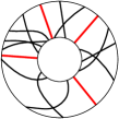
Figure 7: The circular permutation representation $C$ of a graph with four connected components. The red line segments mark the positions where $C$ can be opened.

If $|CC(H^{\prime})|=1$ or $|CC(H)|=2$ there are only one or two positions, respectively, where we can open $C_{p}^{\prime}$. Hence in these cases we can construct all one or two possible permutation diagrams $D_{p}^{\prime}$ representing $H^{\prime}$ and check whether one of them is extendible. Else we distinguish several further cases.

Case 1: $|CC(H)|>2$ and there exists a vertex $u$ in $G$ such that $u$ has a neighbor in every connected component of $H^{\prime}$ but is not adjacent to all vertices in $H$. Note that if more than two connected components in $CC(H^{\prime})$ contain vertices not adjacent to $u$, $C^{\prime}_{p}$ is not extendible. The same holds if two non-adjacent connected components in $CC(H^{\prime})$ contain vertices not adjacent to $u$. Else we distinguish further subcases.

Case 1a: Two connected components in $CC(H^{\prime})$ contain vertices not adjacent to $u$ and the corresponding blocks are adjacent in $C_{p}^{\prime}$. Then the only position where we can open $C_{p}^{\prime}$ is between these two blocks.

Case 1b: Only one connected components in $CC(H^{\prime})$ contains vertices not adjacent to $u$. Then we can either open to the left or to the right of the block. In this case we check whether one of the to possibilities gives us an extendible permutation diagram.

Case 2: there exists no vertex $u$ in $G$ that has a neighbor in every connected component of $H^{\prime}$ but is not adjacent to every vertex in $H$. Then we remove all vertices from $G$ that are adjacent to every other vertex in $H$. If $G$ is empty afterwards, we can choose an arbitrary gap between two adjacent blocks and open $C_{p}^{\prime}$ there. Else we iteratively merge for each remaining vertex $u$ all connected components of $H^{\prime}$ that contain a vertex adjacent to $u$. Since $G$ is connected we end up with either one or two blocks which gives us only one or two positions to open $C_{p}^{\prime}$, respectively. We check whether one of them leads to an extendible permutation diagram.

6.2 The Simultaneous Representation Problem

In this section we show that $\textsc{SimRep${}^{\star}$}(\textsc{CPerm})$ can be solved via a quadratic-time Turing reduction to SimRep^⋆ (Perm) using the switch operation. Here we need to switch the neighborhood of a vertex v shared by all input graphs. Hence in contrast to the reduction in Section 6.1, where we switched the neighborhood of a vertex of minimum degree, the graph $G_{N(v)}$ may have quadratic size.

Lemma 6.3.

Let $G_{1},G_{2},\dots,G_{r}$ be sunflower circular permutation graphs sharing an induced subgraph $H$. Let $v$ be a vertex in $H$ and let $G_{i}^{\prime}$ be the graph we obtain by switching all neighbors of vertex $v$ in $G_{i}$ for $i\in\{1,\dots,r\}$. Then $G_{1},G_{2},\dots,G_{r}$ are simultaneous circular permutation graphs if and only if $G_{1}^{\prime},G_{2}^{\prime},\dots,G_{r}^{\prime}$ are simultaneous permutation graphs.

Proof 6.4.

Recall that $G_{1}^{\prime},G_{2}^{\prime},\dots,G_{r}^{\prime}$ are indeed permutation graphs [35]. Let $G_{1},G_{2},\dots,G_{r}$ be simultaneous circular permutation graphs. Then there exist circular permutation diagrams $C_{1},C_{2},\dots,C_{r}$ such that for every $1\leq i\leq r$, $C_{i}$ represents $G_{i}$ and all $C_{i}$s coincide restricted to the vertices of $H$. We get a circular permutation diagram $C_{i}^{\prime}$ representing $G_{i}^{\prime}$ by switching all chords corresponding to neighbors of vertex $v$ in $C_{i}$. Since the order of the vertices along the inner and outer circle is not affected by the switch operation, we know that all $C_{i}^{\prime}$s coincide restricted to the vertices of $H$. Recall that after switching all neighbors of chord $v$ in a circular permutation diagram, no chord intersects $v$ any more and hence we obtain a permutation diagram $D_{i}^{\prime}$ representing $G_{i}^{\prime}$ by opening $C_{i}^{\prime}$ along the chord $v$. Then the $D_{i}^{\prime}$s also coincide on the vertices of $H$ and hence $G_{1}^{\prime},G_{2}^{\prime},\dots,G_{r}^{\prime}$ are simultaneous permutation graphs.

Conversely let $G_{1}^{\prime},G_{2}^{\prime},\dots,G_{r}^{\prime}$ be simultaneous permutation graphs. Then there exist permutation diagrams $D_{1}^{\prime},D_{2}^{\prime},\dots,D_{r}^{\prime}$ such that for every $1\in\{1,\dots,r\}$, $D_{i}^{\prime}$ represents $G_{i}^{\prime}$ and all $D_{i}^{\prime}$s coincide on the vertices of $H$. Recall that we can transform every linear permutation diagram $D_{i}^{\prime}$ into a circular permutation diagram $C_{i}^{\prime}$ representing $G_{i}^{\prime}$. Note that the $C_{i}^{\prime}$s also coincide on the vertices of $H$. Now we obtain a circular permutation diagram $C_{i}$ representing $G_{i}$ by switching all chords that correspond to vertices adjacent to $v$. The $C_{i}$s still coincide on the vertices of $H$ since the switch operation does not change the order of the vertices along the outer or the inner circle of a circular permutation diagram and chords corresponding to vertices in $H$ are either switched in every $C_{i}$ or in none of them.

Theorem 6.5.

$\textsc{SimRep${}^{\star}$}(\textsc{CPerm})$ can be solved in $O(n^{2}$) time.

Proof 6.6.

Let $G_{1},\dots,G_{r}$ be sunflower circular permutation graphs. Let $v$ be a vertex in $H$ and let $G_{i}^{\prime}$ be the graph we obtain by switching all neighbors of vertex $v$ in $G_{i}$ for $i\in\{1,\dots,r\}$. By Lemma 6.3 to solve SimRep(CPerm) for $G_{1},G_{2},\dots,G_{r}$ it suffices to solve SimRep(Perm) for $G_{1}^{\prime},G_{2}^{\prime},\dots,G_{r}^{\prime}$. Computing $G_{1}^{\prime},G_{2}^{\prime},\dots,G_{r}^{\prime}$ takes quadratic time. In Section 5.2 we have seen that SimRep(perm) can be solved in linear time for sunflower permutation graphs $G_{1}^{\prime},\dots,G_{r}^{\prime}$, hence in total we need quadratic time to solve $\textsc{SimRep${}^{\star}$}(\textsc{CPerm})$.

If $G_{1},G_{2},\dots,G_{r}$ are simultaneous circular permutation graphs we get corresponding simultaneous representations by transforming simultaneous linear permutation diagrams representing $G_{1}^{\prime},G_{2}^{\prime},\dots,G_{r}^{\prime}$ into circular permutation diagrams and switching all chords corresponding to a neighbor of vertex $v$ in $H$. This takes quadratic time in total.

7 Simultaneous Orientations and Representations for General Comparability Permutation Graphs

We show that the simultaneous orientation problem for comparability graphs and the simultaneous representation problem for permutation graphs are NP-complete in the non-sunflower case.

Theorem 7.1.

SimOrient for $k$ comparability graphs where $k$ is part of the input is NP-complete.

Proof 7.2.

Clearly the problem is in NP.

To show the NP-hardness, we give a reduction from the known NP-complete problem TotalOrdering [33], which is defined as follows. Given a finite set $S$ and a finite set $T$ of triples of elements in $S$, decide whether there exists a total ordering $<$ of $S$ such that for all triples $(x,y,z)\in T$ either  $x<y<z$ or $x>y>z$. Let $H_{T}$ be an instance of TotalOrdering with $s=|S|$ and $t=|T|$. We number the triples in $T$ with $1,\dots,t$ and denote the $i$th triple by  $(x_{i},y_{i},z_{i})$. We construct an instance $H_{S}$ of SimOrient, consisting of undirected graphs $G_{0},\dots,G_{t}$ as follows.

• $G_{0}:=(S,E_{0})$ is the complete graph with one vertex for each element in $S$.

• $G_{i}:=(V_{i},E_{i})$ for $1\leq i\leq t$ is the graph with vertex set $V_{i}=\{x_{i},y_{i},z_{i},a_{i},b_{i}\}$, where $a_{i},b_{i}\notin S$ are new vertices, and edges $E_{i}=\{x_{i}a_{i},x_{i}y_{i},x_{i}z_{i},$ $y_{i}z_{i},z_{i}b_{i}\}$; see Figure 8.

Figure 8: The (permutation) graph $G_{i}$ corresponding to the $i-th$ triple $(x_{i},y_{i},z_{i})$ of a TotalOrdering instance with corresponding permutation diagram.

For every $1\leq i\leq t$, the graph $G_{i}$ has exactly two transitive orientations, namely $\{\overrightarrow{x_{i}a_{i}},\overrightarrow{x_{i}y_{i}},$ $\overrightarrow{x_{i}z_{i}},\overrightarrow{y_{i}z_{i}},\overrightarrow{b_{i}z_{i}}\}$ and its reversal. We now have to show that $H_{T}$ has a solution if and only if $G_{0},\dots,G_{t}$ are simultaneous comparability graphs.

First, assume that $G_{0},\dots,G_{t}$ are simultaneous comparability graphs. Hence there exist orientations $T_{0},\dots,T_{t}$ such that for every $0\leq i\leq t$, $T_{i}$ is an orientation of $G_{i}$ and for every $j,k\in\{0,\dots t\}$ every edge in $E_{j}\cap E_{k}$ is oriented in the same way in both $T_{j}$ and $T_{k}$. Then the orientation of the complete graph $G_{0}$ implies a total order on the elements of $T$, where $u<v$ if and only if the edge $uv$ is oriented from $u$ to $v$. By construction, there are only two valid transitive orientations for $G_{i}$. The one given above implies $x_{i}<y_{i}<z_{i}$ and for the reverse orientation we get $z_{i}<y_{i}<x_{i}$. Hence the received total order satisfies that for every triple $(x,y,z)\in T$ we have either $x<y<z$ or $x>y>z$.

Conversely, assume that $H_{T}$ has a solution. Then there exists a total order $<$ such that for all triples  $(x,y,z)\in T$ either $x<y<z$ or $x>y>z$ holds. We get a transitive orientation $T_{i}$ of $G_{i}$ for $1\leq i\leq t$ by orienting all edges between the vertices $x_{i},y_{i}$ and $z_{i}$ towards the greater element according to the order $<$. If $x_{i}$ is the smallest element of the triple, then we choose $\overrightarrow{x_{i}a_{i}}$ and $\overrightarrow{b_{i}z_{i}}$, else $z_{i}$ is the smallest element and we choose $\overrightarrow{a_{i}x_{i}}$ and $\overrightarrow{z_{i}b_{i}}$. Finally, we orient the edges in $G_{0}$ also towards the greater element according to $<$. This gives us orientations $T_{0},\dots,T_{t}$ of $G_{0},\dots,G_{t}$ with the property that for every $j,k\in\{0,\dots t\}$ every edge in $E_{j}\cap E_{k}$ is oriented in the same way in both $T_{j}$ and $T_{k}$. Hence $G_{0},\dots,G_{t}$ are simultaneous comparability graphs.

Hence the instance $H_{T}$ of TotalOrdering has a solution if and only if the instance $H_{S}$ is a yes-instance of SimOrient. Since $H_{S}$ can be constructed from $H_{T}$ in polynomial time, it follows that SimOrient is NP-complete.

Theorem 7.3.

SimRep(Perm) for $k$ permutation graphs where $k$ is not fixed is NP-complete.

Proof 7.4.

Clearly the problem is in NP.

To show the NP-hardness, we use the same reduction as in the proof of Theorem 7.1. Let $H_{T}$ be the corresponding instance of TotalOrdering. Note that $G_{0},\dots,G_{t}$ are permutation graphs and thus $\overline{G_{0}},\dots,\overline{G_{t}}$ are comparability graphs.. We already know that $H_{T}$ has a solution if and only if $G_{0},\dots,G_{t}$ are simultaneous comparability graphs. Hence it remains to show that $G_{0},\dots,G_{t}$ are simultaneous co-comparability graphs if $H_{T}$ has a solution. Note that $E(\overline{G_{0}})=\emptyset$ and for every $1\leq i\leq t$ for every edge $uv\in E(\overline{G_{i}})$ at least one of the endpoints $u$ and $v$ is in $\{a_{i},b_{i}\}$. Hence, $\overline{G_{0}},\dots,\overline{G_{t}}$ pairwise do not share any edges and thus they are also simultaneous comparability graphs.

8 Conclusion

We showed that the orientation extension problem and the simultaneous orientation problem for sunflower comparability graphs can be solved in linear time using the concept of modular decompositions. Further we were able to use these algorithms to solve the partial representation problem for permutation and circular permutation graphs and the simultaneous representation problem for sunflower permutation graphs also in linear time. For the simultaneous representation problem for circular permutation graphs we gave a quadratic-time algorithm. The non-sunflower case of the simultaneous orientation problem and the simultaneous representation problem turned out to be NP-complete.

It remains an open problem whether the simultaneous representation problem for sunflower circular permutation graphs can be solved in subquadratic time. Furthermore it would be interesting to examine whether the concept of modular decomposition is also applicable to solve the partial representation and the simultaneous representation problem for further graph classes, e.g. trapezoid graphs. There may also be other related problems that can be solved for comparability, permutation and circular permutation graphs with the concept of modular decompositions.

References

- [1] Patrizio Angelini, Giuseppe Di Battista, Fabrizio Frati, Vít Jelínek, Jan Kratochvíl, Maurizio Patrignani, and Ignaz Rutter. Testing planarity of partially embedded graphs. ACM Transactions on Algorithms, 11(4):32:1–32:42, 2015.
- [2] Patrizio Angelini, Giordano Da Lozzo, and Daniel Neuwirth. On some -complete SEFE problems. In Sudebkumar Prasant Pal and Kunihiko Sadakane, editors, In Proceedings of the 8th International Workshop on Algorithms and Computation (WALCOM’14), volume 8344 of Lecture Notes in Computer Science, pages 200–212. Springer, 2014. doi:10.1007/978-3-319-04657-0_20.
- [3] Bengt Aspvall, Michael F. Plass, and Robert E. Tarjan. A linear-time algorithm for testing the truth of certain quantified boolean formulas. Information Processing Letters, 8(3):121–123, 1979.
- [4] Thomas Bläsius and Ignaz Rutter. Simultaneous PQ-ordering with applications to constrained embedding problems. ACM Transactions on Algorithms, 12(2):16:1–16:46, 2015. doi:10.1145/2738054.
- [5] Thomas Bläsius, Stephen G. Kobourov, and Ignaz Rutter. Simultaneous embedding of planar graphs. In Roberto Tamassia, editor, Handbook of graph drawing and visualization, pages 349–381. CRC press, 2013.
- [6] Jan Bok and Nikola Jedličková. A note on simultaneous representation problem for interval and circular-arc graphs. Computing Research Repository, 2018. URL: https://arxiv.org/abs/1811.04062.
- [7] Kellogg S. Booth. PQ-tree algorithms. PhD thesis, University of California, Berkeley, 1975.
- [8] Kellogg S. Booth and George S. Lueker. Testing for the consecutive ones property, interval graphs, and graph planarity using PQ-tree algorithms. Journal of Computer and System Sciences, 13(3):335–379, 1976.
- [9] Peter Brass, Eowyn Cenek, Cristian A. Duncan, Alon Efrat, Cesim Erten, Dan P. Ismailescu, Stephen G. Kobourov, Anna Lubiw, and Joseph S.B. Mitchell. On simultaneous planar graph embeddings. Computational Geometry, 36(2):117–130, 2007. doi:10.1016/j.comgeo.2006.05.006.
- [10] Steven Chaplick, Paul Dorbec, Jan Kratochvíl, Mickael Montassier, and Juraj Stacho. Contact representations of planar graphs: Extending a partial representation is hard. In Dieter Kratsch and Ioan Todinca, editors, 40th International Workshop on Graph-theoretic concepts in computer science (WG’14), volume 8747 of Lecture Notes in Computer Science, pages 139–151. Springer, 2014.
- [11] Steven Chaplick, Radoslav Fulek, and Pavel Klavík. Extending partial representations of circle graphs. Journal of Graph Theory, 91(4):365–394, 2019.
- [12] Steven Chaplick, Philipp Kindermann, Jonathan Klawitter, Ignaz Rutter, and Alexander Wolff. Extending partial representations of rectangular duals with given contact orientations. In Tiziana Calamoneri and Federico Corò, editors, Proceedings of the 12th International Conference on Algorithms and Complexity, (CIAC ’21), volume 12701 of Lecture Notes in Computer Science, pages 340–353. Springer, 2021. URL: https://doi.org/10.1007/978-3-030-75242-2_24.
- [13] Thomas H. Cormen, Charles E. Leiserson, Ronald L. Rivest, and Clifford Stein. Introduction to Algorithms. MIT press, Cambridge, 2009.
- [14] Eduard Eiben, Robert Ganian, Thekla Hamm, Fabian Klute, and Martin Nöllenburg. Extending partial 1-planar drawings. In Artur Czumaj, Anuj Dawar, and Emanuela Merelli, editors, Proceedings of the 47th International Colloquium on Automata, Languages, and Programming (ICALP’20), volume 168 of LIPIcs, pages 43:1–43:19. Schloss Dagstuhl - Leibniz-Zentrum für Informatik, 2020. doi:10.4230/LIPIcs.ICALP.2020.43.
- [15] Alejandro Estrella-Balderrama, Elisabeth Gassner, Michael Jünger, Merijam Percan, Marcus Schaefer, and Michael Schulz. Simultaneous geometric graph embeddings. In Seok-Hee Hong, Takao Nishizeki, and Wu Quan, editors, Proceedings of 15th International Symposium on Graph Drawing (GD ’07), pages 280–290. Springer, 2008. doi:10.1007/978-3-540-77537-9_28.
- [16] Harold N. Gabow and Robert E. Tarjan. A linear-time algorithm for a special case of disjoint set union. Journal of Computer and System Sciences, 30(2):209–221, 1985.
- [17] Tibor Gallai. Transitiv orientierbare graphen. Acta Mathematica Academiae Scientiarum Hungarica, 18(1-2):25–66, 1967.
- [18] Elisabeth Gassner, Michael Jünger, Merijam Percan, Marcus Schaefer, and Michael Schulz. Simultaneous graph embeddings with fixed edges. In Fedor V. Fomin, editor, 32nd International Workshop on Graph-Theoretic Concepts in Computer Science (WG’06), pages 325–335. Springer, 2006. doi:10.1007/11917496_29.
- [19] Paul C Gilmore and Alan J Hoffman. A characterization of comparability graphs and of interval graphs. Canadian Journal of Mathematics, 16:539–548, 1964.
- [20] Martin Charles Golumbic. Algorithmic Graph Theory and Perfect Graphs. Elsevier, London, 2004.
- [21] Bernhard Haeupler, Krishnam R. Jampani, and Anna Lubiw. Testing simultaneous planarity when the common graph is 2-connected. Journal of Graph Algorithms and Applications, 17(3):147–171, 2013.
- [22] Dov Harel and Robert E. Tarjan. Fast algorithms for finding nearest common ancestors. SIAM Journal on Computing, 13(2):338–355, 1984.
- [23] Krishnam Raju Jampani and Anna Lubiw. Simultaneous interval graphs. In Otfried Cheong, Kyung-Yong Chwa, and Kunsoo Park, editors, Proceedings of the 21st International Symposium on Algorithms and Computation (ISAAC’ 10), pages 206–217. Springer, 2010. URL: https://doi.org/10.1007/978-3-642-17517-6_20.
- [24] Krishnam Raju Jampani and Anna Lubiw. The simultaneous representation problem for chordal, comparability and permutation graphs. Journal of Graph Algorithms and Applications, 16(2):283–315, 2012.
- [25] Vít Jelínek, Jan Kratochvíl, and Ignaz Rutter. A Kuratowski-type theorem for planarity of partially embedded graphs. Computational Geometry, 46(4):466–492, 2013.
- [26] Pavel Klavík, Jan Kratochvíl, Tomasz Krawczyk, and Bartosz Walczak. Extending partial representations of function graphs and permutation graphs. In Leah Epstein and Paolo Ferragina, editors, 20th Annual European Symposium on Algorithms (ESA’12), Lecture Notes in Computer Science, pages 671–682. Springer, 2012.
- [27] Pavel Klavík, Jan Kratochvíl, Yota Otachi, Ignaz Rutter, Toshiki Saitoh, Maria Saumell, and Tomáš Vyskočil. Extending partial representations of proper and unit interval graphs. Algorithmica, 77(4):1071–1104, 2017.
- [28] Pavel Klavík, Jan Kratochvíl, Yota Otachi, and Toshiki Saitoh. Extending partial representations of subclasses of chordal graphs. Theoretical Computer Science, 576:85–101, 2015.
- [29] Pavel Klavík, Jan Kratochvíl, Yota Otachi, Toshiki Saitoh, and Tomáš Vyskočil. Extending partial representations of interval graphs. Algorithmica, 78(3):945–967, 2017.
- [30] Tomasz Krawczyk and Bartosz Walczak. Extending partial representations of trapezoid graphs. In Hans L. Bodlaender and Gerhard J. Woeginger, editors, 43rd International Workshop on Graph-Theoretic Concepts in Computer Science (WG’17), pages 358–371. Springer, 2017.
- [31] Ross M McConnell and Jeremy P Spinrad. Modular decomposition and transitive orientation. Discrete Mathematics, 201(1-3):189–241, 1999.
- [32] Fabien de Montgolfier. Décomposition modulaire des graphes: théorie, extensions et algorithmes. PhD thesis, Montpellier 2 University, 2003.
- [33] Jaroslav Opatrny. Total ordering problem. SIAM Journal on Computing, 8(1):111–114, 1979.
- [34] Maurizio Patrignani. On extending a partial straight-line drawing. International Journal of Foundations of Computer Science, 17(5):1061–1070, 2006.
- [35] Doron Rotem and Jorge Urrutia. Circular permutation graphs. Networks, 12(4):429–437, 1982.
- [36] Ignaz Rutter, Darren Strash, Peter Stumpf, and Michael Vollmer. Simultaneous representation of proper and unit interval graphs. In Michael A. Bender, Ola Svensson, and Grzegorz Herman, editors, 27th Annual European Symposium on Algorithms (ESA’19), volume 144, page 80. Schloss Dagstuhl–Leibniz-Zentrum fuer Informatik, 2019.
- [37] Marcus Schaefer. Toward a theory of planarity: Hanani-Tutte and planarity variants. In 20th International Symposium on Graph Drawing (GD ’12), pages 162–173. Springer, 2012. doi:10.1007/978-3-642-36763-2_15.
- [38] R Sritharan. A linear time algorithm to recognize circular permutation graphs. Networks: An International Journal, 27(3):171–174, 1996.