Local position-space two-nucleon potentials from leading to fourth order of chiral effective field theory

Abstract

We present local, position-space chiral $NN$ potentials through four orders of chiral effective field theory ranging from leading order (LO) to next-to-next-to-next-to-leading order (N³LO, fourth order) of the $\Delta$-less version of the theory. The long-range parts of these potentials are fixed by the very accurate $\pi N$ LECs as determined in the Roy-Steiner equations analysis. At the highest order (N³LO), the $NN$ data below 190 MeV laboratory energy are reproduced with the respectable $\chi^{2}$/datum of 1.45. A comparison of the N³LO potential with the phenomenological Argonne $v_{18}$ (AV18) potential reveals substantial agreement between the two potentials in the intermediate range ruled by chiral symmetry, thus, providing a chiral underpinning for the phenomenological AV18 potential. Our chiral $NN$ potentials may serve as a solid basis for systematic ab initio calculations of nuclear structure and reactions that allow for a comprehensive error analysis. In particular, the order by order development of the potentials will make possible a reliable determination of the truncation error at each order. Our new family of local position-space potentials differs from existing potentials of this kind by a weaker tensor force as reflected in relatively low $D$-state probabilities of the deuteron ($P_{D}\raisebox{-1.29167pt}{\small$\ \stackrel{{\scriptstyle\textstyle<}}{{\sim}}$ }4.0$ % for our N³LO potentials) and predictions for the triton binding energy above 8.00 MeV (from two-body forces alone). As a consequence, our potentials may lead to different predictions when applied to light and intermediate-mass nuclei in ab initio calculations and, potentially, help solve some of the outstanding problems in microscopic nuclear structure.

I Introduction

A primary goal of theoretical nuclear physics is to explain nuclear structure and reactions in terms of the forces between nucleons—in present-day popular jargon dubbed the ab initio approach. The current prevailing belief in the community is that chiral effective field theory (EFT) is best suited to provide those forces, because it can be related to low-energy QCD in a straight-forward way and produces abundant three-nucleon forces (3NFs) needed for any quantitative nuclear structure prediction ME11 ; EHM09 ; HKK19 ; Heb21 .

Since chiral EFT is a low-momentum expansion, most chiral $NN$ potentials of the past have been developed in momentum space–and are non-local. However, this feature makes them unsuitable for a large group of ab initio few- and many-body algorithms, particularly, the ones known as quantum Monte Carlo (QMC) methods Car15 ; Lyn19 . Variational Monte Carlo (VMC) and Green’s Function Monte Carlo (GFMC) techniques provide reliable solutions of the many-body Schrődinger equation for, presently, up to 12 nucleons. Spectra, form factors, transitions, low-energy scattering, and response functions for light nuclei have been successfully calculated using QMC methods PT20 . A further extension, the Auxiliary Field Diffusion Monte Carlo (AFDMC) Car15 ; Lyn19 , additionally samples the spin-isospin degrees of freedom, thus, making possible the study of neutron matter. In summary, QMC techniques have substantially contributed to the progress in ab initio nuclear structure of the past 20+ years, and will continue to do so. Thus, it is important that high-quality nuclear interactions are available for application by these promising many-body methods.

An important advantage of chiral EFT is that it allows for a systematic quantification of the uncertainties of the predictions. For this it is necessary to conduct calculations at different orders of the chiral expansion. However, so far, local chiral $NN$ potentials have been developed only at next-to-next-to-leading order (NNLO) Gez14 or in the hybrid format, NNLO/N³LO Pia15 ; Pia16 , where two-pion exchange (2PE) contributions are included up to NNLO and contact terms up to next-to-next-to-next-to-leading order (N³LO). To make proper uncertainty quantifications possible, local chiral $NN$ potentials at all orders from leading order (LO) to N³LO (and, if necessary, even beyond) are needed. It is the purpose of this work to construct such local $NN$ potentials of high quality and make them available for QMC calculations as well as any other purposes where they can be of use.

We will develop these potentials within the $\Delta$-less theory, which has two degrees of freedom, namely, pions (Goldstone bosons) and nucleons, and does not include a $\Delta(1232)$-isobar degree of freedom. If an explicit $\Delta$-isobar is included in chiral EFT ($\Delta$-full theory ORK94 ; ORK96 ; BKM97 ; KGW98 ; KEM07 ; KGE18 ), then the two-nucleon force (2NF) and 3NF contributions are enhanced at next-to-leading order (NLO), resulting in a smoother convergence when advancing from leading order (LO) to NNLO. However, summing up all contributions at NNLO brings about very similar results for both versions of the theory KEM07 . The predictions of both theories beyond NNLO are expected to be very similar KGE18 . In contrast to recent claims Jia20 , it has been shown in Ref. NEM21 that there is no advantage to the $\Delta$-full theory.

This paper is organized as follows: In Sec. II, we present the expansion of the $NN$ potential through all orders from LO to N³LO. The reproduction of the $NN$ scattering data and the deuteron properties are given in Sec. III. Uncertainty quantification is considered in Sec. IV. Sec. V concludes the paper.

II The chiral $NN$ potential

II.1 Effective Lagrangians

In the $\Delta$-less version of chiral EFT, which is the one we are applying, the relevant degrees o f freedom are pions and nucleons. Consequently, the effective Lagrangian is subdivided into the following pieces,

$${\cal L}_{\rm eff}={\cal L}_{\pi\pi}+{\cal L}_{\pi N}+{\cal L}_{NN}+\,\ldots\,,$$ (1)

where ${\cal L}_{\pi\pi}$ deals with the dynamics among pions, ${\cal L}_{\pi N}$ describes the interaction between pions and a nucleon, and ${\cal L}_{NN}$ contains two-nucleon contact interactions which consist of four nucleon-fields (four nucleon legs) and no meson fields. The ellipsis stands for terms that involve two nucleons plus pions and three or more nucleons with or without pions, relevant for nuclear many-body forces. Since the interactions of Goldstone bosons must vanish at zero momentum transfer and in the chiral limit ($m_{\pi}\rightarrow 0$), the low-energy expansion of the effective Lagrangian is arranged in powers of derivatives and pion masses, implying to following organization:

$${\cal L}_{\pi\pi} = {\cal L}_{\pi\pi}^{(2)}+{\cal L}_{\pi\pi}^{(4)}+\ldots\,,$$ (2)

$${\cal L}_{\pi N} = {\cal L}_{\pi N}^{(1)}+{\cal L}_{\pi N}^{(2)}+{\cal L}_{\pi N}^{(3)}+{\cal L}_{\pi N}^{(4)}+\ldots,$$ (3)

$${\cal L}_{NN} = {\cal L}^{(0)}_{NN}+{\cal L}^{(2)}_{NN}+{\cal L}^{(4)}_{NN}+\ldots\,,$$ (4)

where the superscript refers to the number of derivatives or pion mass insertions (chiral dimension) and the ellipses stand for terms of higher dimensions. We use the heavy-baryon formulation of the Lagrangians, the explicit expressions of which can be found in Ref. ME11 .

II.2 Power counting

Based upon the above Lagrangians, an infinite number of diagrams contributing to the interactions among nucleons can be drawn. Nuclear potentials are defined by the irreducible types of these graphs. By definition, an irreducible graph is a diagram that cannot be separated into two by cutting only nucleon lines. These graphs are then analyzed in terms of powers of $Q$ with $Q=p/\Lambda_{b}$, where $p$ is generic for a momentum (nucleon three-momentum or pion four-momentum) or a pion mass and $\Lambda_{b}\sim m_{\rho}\sim$ 0.7 GeV is the breakdown scale Fur15 . Determining the power $\nu$ has become know as power counting.

Following the Feynman rules of covariant perturbation theory, a nucleon propagator is $p^{-1}$, a pion propagator $p^{-2}$, each derivative in any interaction is $p$, and each four-momentum integration $p^{4}$. This is also known as naive dimensional analysis or Weinberg counting.

Since we use the heavy-baryon formalism, we encounter terms which include factors of $p/M_{N}$, where $M_{N}$ denotes the nucleon mass. We count the order of such terms by the rule

$$p/M_{N}\sim(p/\Lambda_{b})^{2},$$ (5)

for reasons explained in Ref. Wei90 .

Applying some topological identities, one obtains for the power of a connected irreducible diagram involving $A$ nucleons ME11 ; Wei90

$$\nu=-2+2A-2C+2L+\sum_{i}\Delta_{i}\,,$$ (6)

with

$$\Delta_{i}\equiv d_{i}+\frac{n_{i}}{2}-2\,,$$ (7)

where $L$ denotes the number of loops in the diagram; $d_{i}$ is the number of derivatives or pion-mass insertions and $n_{i}$ the number of nucleon fields (nucleon legs) involved in vertex $i$; the sum runs over all vertexes $i$ contained in the connected diagram under consideration. Note that $\Delta_{i}\geq 0$ for all interactions allowed by chiral symmetry.

An important observation from power counting is that the powers are bounded from below and, specifically, $\nu\geq 0$. This fact is crucial for the convergence of the low-momentum expansion.

For an irreducible $NN$ diagram ($A=2$, $C=1$), the power formula collapses to the very simple expression

$$\nu=2L+\sum_{i}\Delta_{i}\,,$$ (8)

which is most relevant for our current work.

In summary, the chief point of the chiral perturbation theory (ChPT) expansion of the potential is that, at a given order $\nu$, there exists only a finite number of graphs. This is what makes the theory calculable. The expression $(p/\Lambda_{b})^{\nu+1}$ provides an estimate of the relative size of the contributions left out and, thus, of the relative uncertainty at order $\nu$. The ability to calculate observables (in principle) to any degree of accuracy gives the theory its predictive power.

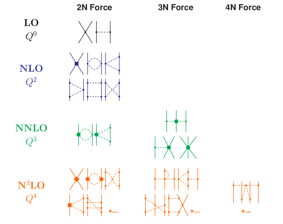
Figure 1: Hierarchy of nuclear forces in ChPT. Solid lines represent nucleons and dashed lines pions. Small dots, large solid dots, solid squares, and solid diamonds denote vertexes of index $\Delta_{i}=\,$ 0, 1, 2, and 4, respectively. $Q=p/\Lambda_{b}$ with $p$ a momentum or pion mass and $\Lambda_{b}$ the breakdown scale. Further explanations are given in the text.

ChPT and power counting imply that nuclear forces evolve as a hierarchy controlled by the power $\nu$, see Fig. 1 for an overview. In what follows, we will focus on the 2NF.

II.3 The long-range $NN$ potential

The long-range part of the $NN$ potential is built up from pion exchanges, which are ruled by chiral symmetry. The various pion-exchange contributions are best analyzed by the number of pions being exchanged between the two nucleons:

$$V_{\pi}=V_{1\pi}+V_{2\pi}+V_{3\pi}+\ldots\,,$$ (9)

where the meaning of the subscripts is obvious and the ellipsis represents $4\pi$ and higher pion exchanges. For each of the above terms, we have a low-momentum expansion:

$$V_{1\pi} = V_{1\pi}^{(0)}+V_{1\pi}^{(2)}+V_{1\pi}^{(3)}+V_{1\pi}^{(4)}+\ldots\,,$$ (10)

$$V_{2\pi} = V_{2\pi}^{(2)}+V_{2\pi}^{(3)}+V_{2\pi}^{(4)}+\ldots\,,$$ (11)

$$V_{3\pi} = V_{3\pi}^{(4)}+\ldots\,,$$ (12)

where the superscript denotes the order $\nu$ of the expansion. Higher order corrections to the one-pion exchange (1PE) are taken care of by mass and coupling constant renormalizations. Note also that, on shell, there are no relativistic corrections. Thus, $V_{1\pi}=V_{1\pi}^{(0)}$ through all orders. The leading $3\pi$-exchange contribution that occurs at N³LO, $V_{3\pi}^{(4)}$, has been calculated in Refs. Kai00a ; Kai00b and found to be negligible. We, therefore, omit it.

Order by order, the long-range $NN$ potential then builds up as follows:

$$V_{\pi}^{\rm LO} = V_{1\pi}^{(0)}\,,$$ (13)

$$V_{\pi}^{\rm NLO} = V_{\pi}^{\rm LO}+V_{2\pi}^{(2)}\,,$$ (14)

$$V_{\pi}^{\rm NNLO} = V_{\pi}^{\rm NLO}+V_{2\pi}^{(3)}\,,$$ (15)

$$V_{\pi}^{\rm N3LO} = V_{\pi}^{\rm NNLO}+V_{2\pi}^{(4)}\,.$$ (16)

We note that we add to $V_{\pi}^{\rm N3LO}$ the $1/M_{N}$ corrections of the NNLO 2PE proportional to $c_{i}$ (cf. Table 1). This correction is proportional to $c_{i}/M_{N}$ (cf. Fig. 9 and Appendix A.5, below) and appears nominally at fifth order, but we include it at fourth order. As demonstrated in Ref. EM02 , the 2PE football diagram proportional to $c_{i}^{2}$ that appears at N³LO (Fig. 8(a) and Appendix A.4.1) is unrealistically attractive, while the $c_{i}/M_{N}$ correction is large and repulsive. Therefore, it makes sense to group these diagrams together to arrive at a more realistic intermediate-range attraction at N³LO. This is common practice and has been done so in Refs. EM03 ; EKM15 ; EMN17 .

The explicit mathematical expressions for the pion-exchanges up to N³LO are very involved. We have, therefore, moved them into the Appendix A.

Table 1: The $\pi N$ LECs as determined in the Roy-Steiner-equation analysis of $\pi N$ scattering conducted in Ref. Hof15 . The given orders of the chiral expansion refer to the $NN$ system. The $c_{i}$ and $\bar{d}_{i}$ are the LECs of the second and third order $\pi N$ Lagrangian ME11 and are in units of GeV^-1 and GeV^-2, respectively. The uncertainties in the last digits are given in parentheses after the values. We use the central values.

	NNLO	N3LO
$c_{1}$	–0.74(2)	–1.07(2)
$c_{2}$		3.20(3)
$c_{3}$	–3.61(5)	–5.32(5)
$c_{4}$	2.44(3)	3.56(3)
$\bar{d}_{1}+\bar{d}_{2}$		1.04(6)
$\bar{d}_{3}$		–0.48(2)
$\bar{d}_{5}$		0.14(5)
$\bar{d}_{14}-\bar{d}_{15}$		–1.90(6)

Chiral symmetry establishes a link between the dynamics in the $\pi N$-system and the $N\!N$-system through common low-energy constants (LECs). Therefore, consistency requires that we use the LECs for subleading $\pi N$-couplings as determined in the analysis of low-energy $\pi N$-scattering. Currently, the most reliable $\pi N$ analysis is the one by Hoferichter and Ruiz de Elvira et al. Hof15 , in which the Roy-Steiner equations are applied. These LECs carry very small uncertainties (cf. Table 1); in fact, the uncertainties are so small that they are negligible for our purposes. This makes the variation of the $\pi N$ LECs in $NN$ potential construction obsolete and reduces the error budget in applications of these potentials. For the potentials constructed in this paper, the central values of Table 1 are applied. Other constants involved in our potential construction are shown in Table 2.

Table 2: Basic constants used throughout this work PDG .

quantity		Value
Axial-vector coupling constant $g_{A}$		1.29
Pion-decay constant $f_{\pi}$		92.4 MeV
Charged-pion mass $m_{\pi^{\pm}}$		139.5702 MeV
Neutral-pion mass $m_{\pi^{0}}$		134.9766 MeV
Average pion-mass $\bar{m}_{\pi}$		138.0390 MeV
Proton mass $M_{p}$		938.2720 MeV
Neutron mass $M_{n}$		939.5654 MeV
Average nucleon-mass $\bar{M}_{N}$		938.9183 MeV
Conversion constant $\hbar c$		197.32698 MeV fm

II.4 The short-range $NN$ potential

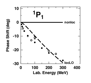
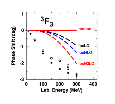
Figure 2: Left panel: ${}^{1}P_{1}$ phase shifts for the order zero (i.e., LO) contact terms with nonlocal regulator (solid black line, “nonloc”) versus the same terms multiplied with a local regulator (dashed black line, “locLO”). Right panel: ${}^{3}F_{3}$ phase shifts for the central force contact terms at orders LO, NLO, and N³LO with nonlocal regulator (solid red line, “nonloc”) versus the same terms multiplied with a local regulator (dashed lines at orders as denoted). The central force contact LECs of the N³LO potential with cutoff combination $(R_{\pi},R_{\rm ct})$=$(1.0,0.70)$ fm are applied (Table 7). The filled and open circles represent the results from the Nijmegen multi-energy $np$ phase-shift analysis Sto93 and the GWU single-energy $np$ analysis SP07 SP07 , respectively.

The short-range $NN$ potential is described by contributions of the contact type, which are constrained by parity, time-reversal, and the usual invariances, but not by chiral symmetry. Because of parity and time-reversal only even powers of momentum are allowed. Thus, the expansion of the contact potential is formally written as

$$V_{\rm ct}=V_{\rm ct}^{(0)}+V_{\rm ct}^{(2)}+V_{\rm ct}^{(4)}+\ldots\;,$$ (17)

where the superscript denotes the power or order.

In principle, the most general set of contact terms at each order is provided by all combinations of spin, isospin, and momentum operators that are allowed by the usual symmetries OM58 at the given order. Two momenta are available, namely, the final and initial nucleon momenta in the center-of-mass system, ${\vec{p}}\,^{\prime}$ and $\vec{p}$. This can be reformulated in terms of two alternative momenta, viz., the momentum transfer $\vec{q}={\vec{p}}\,^{\prime}-\vec{p}$ and the average momentum $\vec{k}=({\vec{p}}\,^{\prime}+\vec{p})/2$. Functions of $\vec{q}$  lead to local interactions, that is, to functions of the relative distance ${\vec{r}}$ between the two nucleons after Fourier transform. On the other hand, functions of $\vec{k}$ lead to nonlocal interactions.

Since ChPT is a low-momentum expansion, it requires cutting off high momenta to avoid divergences. This is achieved by multiplying the potential with a regulator function that suppresses the large momenta (or, equivalently, the short distances). Depending on the type of momenta used, the regulator can be local or nonlocal.

When chiral $NN$ potentials are constructed in momentum-space and regulated by nonlocal cutoff functions ME11 , then it is possible to reduce the number of contact operators (by a factor of two) due to Fierz ambiguity Fie37 ; Hut17 , which is a consequence of the fact that nucleons are Fermions and obey the Pauli exclusion principle. However, for the reasons stated in the Introduction, we wish to construct $NN$ potentials which are strictly local, implying that we have to use local regulators.

When a local (regulator) function is applied to the contact terms, then the Fierz rearrangemnt freedom is violated Hut17 . To provide a simple example of this, consider a contact operator of order zero ($\sim Q^{0}$, LO). After a partial-wave decomposition and when multiplied by either no regulator or a nonlocal regulator, such operator produces no contributions for states with orbital angular momentum $L>0$, i.e., $P$ and higher partial waves. However, this property is violated when the operator is multiplied with a local regulator function Hut17 . We demonstrate this fact in Fig. 2, where, in the left panel, we show phase shifts in the ${}^{1}P_{1}$ state: The solid line (“nonloc”) shows the phase shifts when the LO contact terms are multiplied with a nonlocal cutoff function, which does not violate Fierz ambiguity and, therefore, the phase shifts are zero. However, when the LO contact terms are multiplied by a local regulator, the dashed curve (“locLO”) is obtained—obviously a severe violation. This violation by local regulators continues through higher orders. As an example, we show in the right panel of Fig. 2 the phase shifts in an $F$-wave, where polynomial terms up to fourth order should not contribute which, as demonstrated in the figure, is, indeed, true when a nonlocal cutoff is multiplied to contact terms up to fourth order (solid red curve, “nonloc”). However, when local functions are applied, then at orders $Q^{0}$, $Q^{2}$, and $Q^{4}$, the contributions are not zero anymore as demonstrated by the dashed curves denoted by “locLO”, “locNLO”, “locN3LO”, respectively; which, again, may be perceived as a severe violation of the Fierz rearrangement freedom.

Attempts can be undertaken to restore Fierz reordering as tried in Ref. Hut17 by way of contributions of higher order. However, the Fierz violations demonstrated in Fig. 2 for ${}^{3}F_{3}$ cannot be compensated within the scope of this work, since they would require contributions of sixth order.

To make a long story short, our bottom-line argument is simply that it does not make sense to apply a symmetry that is invalid for the problem under consideration. Therefore, we will not apply Fierz reordering to the contact terms and, hence, use for the contacts all combinations of spin, isospin, angular momentum, and momentum $\vec{q}$ that are allowed by the usual symmetries, for each of the given orders. On a historical note, this is also the approach that was taken for the very first chiral $NN$ potentials ever constructed ORK94 ; ORK96 .

According to standard power counting rules, only two contacts are needed at LO while, in our approach and the one of Refs. ORK94 ; ORK96 , there are four at LO. Consequently, the approach uses an overcomplete basis implying that some parameters are redundant. Note, however, that there is nothing fundamentally wrong with using redundant parameters. It merely means that the approach may be perceived as being inefficient (which is not the same as being wrong). Ironically, here, the inefficient approach is more efficient, since it allows to relate the contact parameters in a one-to-one correspondence to states of well-defined total spin $S$ and total isospin $T$ [Eqs. (163) and (164)] and, thus, makes possible fitting phase shifts state-by-state. However, as discussed, due to the local character of the regulator function, Eq. (19), that is multiplied to the zero-order contacts, $P$ and higher partial waves will be affected by LO contact terms (cf.  Fig. 2), hence, promoting higher order terms to LO and increasing the fit freedom when four independent LO parameters are available.

At higher orders, the discussed redundancy applies to the $C_{8}$ term at NLO and the $D_{10}$, $D_{12}$, and $D_{14}$ terms at N³LO (see below for the detailed expressions). As a result, at N³LO we have only 11 non-redundant contact parameters, even though according to power counting rules there should be 15. The four “missing” fourth order contact terms are nonlocal (cf. Ref. Pia15 ) and, therefore, we have to leave them out, as practiced already in Ref. Pia16 .

Our approach overlaps with the philosophy of the Argonne $v_{18}$ potential (AV18) WSS95 , which includes 14 charge-independent operators. Not accidentally, we will also have 14 contact operators at N³LO (see below) which are all equivalent to the 14 operators of the AV18 potential. This fact provides another advantage to our approach, namely, there is now a one-to-one correspondence between the terms of the AV18 potential and the chiral potentials of this paper. This allows for a detailed comparison between the two potentials as conducted in Appendix C, which turns out to be most revealing.

Next, we present the explicit expressions for the contact operators, order by order.

II.4.1 Leading order

In momentum-space, the LO or zeroth order charge-independent contact terms are given by

$${V}_{\rm ct}^{(0)}(q)\, = \,\left(C_{c}\,+C_{\tau}\,\bm{\tau}_{1}\cdot\bm{\tau}_{2}\,+\,C_{\sigma}\,\vec{\sigma}_{1}\cdot\vec{\sigma}_{2}\,+\,C_{\sigma\tau}\,\vec{\sigma}_{1}\cdot\vec{\sigma}_{2}\;\bm{\tau}_{1}\cdot\bm{\tau}_{2}\right)\,f_{\rm ct}(q)$$ (18)

with regulator function

$$f_{\rm ct}(q)=e^{-(q/\Lambda)^{2}}$$ (19)

and $\Lambda$ a momentum cutoff. The operators $\vec{\sigma}_{1,2}$ and $\bm{\tau}_{1,2}$ denote the spin and isospin operators for nucleon 1 and 2, respectively, with $\bm{\tau}_{i}=(\tau_{ix},\tau_{iy},\tau_{iz})$, $i=1,2$. In the convention we apply, the proton carries an eigenvalue of $(+1)$ and the neutron an eigenvalue of $(-1)$ with regard to $\tau_{z}$.

At LO, we also include charge-dependent contact terms that are defined as follows:

$${}^{\rm CD}V_{\rm ct}^{(0)}(q)\, = \,\left[C_{T_{12}}^{\rm CD}\,T_{12}\,+\,C_{\sigma T_{12}}^{\rm CD}\,\vec{\sigma}_{1}\cdot\vec{\sigma}_{2}\,T_{12}+\,C_{\tau_{z}}^{\rm CA}\,(\tau_{1z}+\tau_{2z})\,+\,C_{\sigma\tau_{z}}^{\rm CA}\,\vec{\sigma}_{1}\cdot\vec{\sigma}_{2}\,(\tau_{1z}+\tau_{2z})\right]\,f_{\rm ct}(q)\,,$$ (20)

with

$$T_{12}=3\,\tau_{1z}\tau_{2z}-\bm{\tau}_{1}\cdot\bm{\tau}_{2}$$ (21)

an isotensor operator. Terms proportional to $T_{12}$ are charge dependent, while terms proportional to $(\tau_{1z}+\tau_{2z})$ are charge asymmetric.

In position space, this translates into

$$\widetilde{V}_{\rm ct}^{(0)}(r)\, = \,\left(C_{c}\,+C_{\tau}\,\bm{\tau}_{1}\cdot\bm{\tau}_{2}\,+\,C_{\sigma}\,\vec{\sigma}_{1}\cdot\vec{\sigma}_{2}\,+\,C_{\sigma\tau}\,\vec{\sigma}_{1}\cdot\vec{\sigma}_{2}\;\bm{\tau}_{1}\cdot\bm{\tau}_{2}\right)\,^{\rm ct}\widetilde{V}_{C}^{(0)}(r)$$ (22)

and

$${}^{\rm CD}\widetilde{V}_{\rm ct}^{(0)}(r)\, = \,\left[C_{T_{12}}^{\rm CD}\,T_{12}\,+\,C_{\sigma T_{12}}^{\rm CD}\,\vec{\sigma}_{1}\cdot\vec{\sigma}_{2}\,T_{12}+\,C_{\tau_{z}}^{\rm CA}\,(\tau_{1z}+\tau_{2z})\,+\,C_{\sigma\tau_{z}}^{\rm CA}\,\vec{\sigma}_{1}\cdot\vec{\sigma}_{2}\,(\tau_{1z}+\tau_{2z})\right]^{\rm ct}\widetilde{V}_{C}^{(0)}(r)$$ (23)

with

$${}^{\rm ct}\widetilde{V}_{C}^{(0)}(r)=\widetilde{f}_{\rm ct}(r)=\frac{1}{\pi^{3/2}\,R_{\rm ct}^{3}}\,e^{-(r/R_{\rm ct})^{2}}\,,$$ (24)

the Fourier transform of $f_{\rm ct}(q)$, and $R_{\rm ct}=2/\Lambda$. Note that we use units such that $\hbar=c=1$.

II.4.2 Next-to-leading order

In momentum-space, the NLO or second order contact contribution is

$${V}_{\rm ct}^{(2)}({\vec{p}}~{}^{\prime},\vec{p})\, = \Big{\{}\left(C_{1}\,+C_{2}\,\bm{\tau}_{1}\cdot\bm{\tau}_{2}\,+\,C_{3}\,\vec{\sigma}_{1}\cdot\vec{\sigma}_{2}\,+\,C_{4}\,\vec{\sigma}_{1}\cdot\vec{\sigma}_{2}\;\bm{\tau}_{1}\cdot\bm{\tau}_{2}\right)\,q^{2}$$ (25)

$$+\left(C_{5}\,+C_{6}\,\bm{\tau}_{1}\cdot\bm{\tau}_{2}\,\right)\,\widehat{S}_{12}(\vec{q})\;\;$$

$$+\left(C_{7}\,+C_{8}\,\bm{\tau}_{1}\cdot\bm{\tau}_{2}\,\right)\,\left[-i\vec{S}\cdot(\vec{q}\times\vec{k})\,\right]\Big{\}}\,f_{\rm ct}(q)\,,$$

where $\vec{S}=(\vec{\sigma}_{1}+\vec{\sigma}_{2})/2$ denotes the total spin and

$$\widehat{S}_{12}(\vec{q})=3\,\vec{\sigma}_{1}\cdot\vec{q}\,\,\>\vec{\sigma}_{2}\cdot\vec{q}-q^{2}\,\vec{\sigma}_{1}\cdot\vec{\sigma}_{2}$$ (26)

is the spin-tensor operator in momentum-space.

Fourier transform of the above creates the second order contact contribution in position space

$$\widetilde{V}_{\rm ct}^{(2)}(\vec{r})\, = \,\left(C_{1}\,+C_{2}\,\bm{\tau}_{1}\cdot\bm{\tau}_{2}\,+\,C_{3}\,\vec{\sigma}_{1}\cdot\vec{\sigma}_{2}\,+\,C_{4}\,\vec{\sigma}_{1}\cdot\vec{\sigma}_{2}\;\bm{\tau}_{1}\cdot\bm{\tau}_{2}\right)\,\,^{\rm ct}\widetilde{V}_{C}^{(2)}(r)$$ (27)

$$+\left(C_{5}\,+C_{6}\,\bm{\tau}_{1}\cdot\bm{\tau}_{2}\,\right)\,S_{12}(\hat{r})\;\;^{\rm ct}\widetilde{V}_{T}^{(2)}(r)$$

$$+\left(C_{7}\,+C_{8}\,\bm{\tau}_{1}\cdot\bm{\tau}_{2}\,\right)\,(\vec{L}\cdot\vec{S})\;\;^{\rm ct}\widetilde{V}_{LS}^{(2)}(r)\,,$$

where

$$S_{12}(\hat{r})=3\vec{\sigma}_{1}\cdot\hat{r}\,\,\>\vec{\sigma}_{2}\cdot\hat{r}-\vec{\sigma}_{1}\cdot\vec{\sigma}_{2}$$ (28)

denotes the standard position-space spin-tensor operator with $\hat{r}=\vec{r}/r$, and $\vec{L}$ is the operator of total angular momentum. Furthermore,

$${}^{\rm ct}\widetilde{V}_{C}^{(2)}(r) = -\widetilde{f}_{\rm ct}^{(2)}(r)-\frac{2}{r}\,\widetilde{f}_{\rm ct}^{(1)}(r)\,,$$ (29)

$${}^{\rm ct}\widetilde{V}_{T}^{(2)}(r) = -\widetilde{f}_{\rm ct}^{(2)}(r)+\frac{1}{r}\,\widetilde{f}_{\rm ct}^{(1)}(r)\,,$$ (30)

$${}^{\rm ct}\widetilde{V}_{LS}^{(2)}(r) = -\frac{1}{r}\,\widetilde{f}_{\rm ct}^{(1)}(r)\,,$$ (31)

with

$$\widetilde{f}_{\rm ct}^{(n)}(r)=\frac{d^{n}\widetilde{f}_{\rm ct}(r)}{dr^{n}}\,.$$ (32)

II.4.3 Next-to-next-to-next-to-leading order

In momentum-space, the N³LO or fourth order contact contribution is assumed to be

$${V}_{\rm ct}^{(4)}({\vec{p}}~{}^{\prime},\vec{p})\, = \Big{\{}\left(D_{1}\,+D_{2}\,\bm{\tau}_{1}\cdot\bm{\tau}_{2}\,+\,D_{3}\,\vec{\sigma}_{1}\cdot\vec{\sigma}_{2}\,+\,D_{4}\,\vec{\sigma}_{1}\cdot\vec{\sigma}_{2}\;\bm{\tau}_{1}\cdot\bm{\tau}_{2}\right)\,q^{4}$$ (34)

$$+\left(D_{5}\,+D_{6}\,\bm{\tau}_{1}\cdot\bm{\tau}_{2}\,\right)\,q^{2}\,\widehat{S}_{12}(\vec{q})\;\;$$

$$+\left(D_{7}\,+D_{8}\,\bm{\tau}_{1}\cdot\bm{\tau}_{2}\,\right)\,q^{2}\,\left[-i\vec{S}\cdot(\vec{q}\times\vec{k})\,\right]\;\;$$

$$+\left(D_{9}\,+D_{10}\,\bm{\tau}_{1}\cdot\bm{\tau}_{2}\,\right)\,\left[-i\vec{S}\cdot(\vec{q}\times\vec{k})\,\right]^{2}$$

$$+\,\left(D_{11}\,+D_{12}\,\bm{\tau}_{1}\cdot\bm{\tau}_{2}\,+\,D_{13}\,\vec{\sigma}_{1}\cdot\vec{\sigma}_{2}\,+\,D_{14}\,\vec{\sigma}_{1}\cdot\vec{\sigma}_{2}\;\bm{\tau}_{1}\cdot\bm{\tau}_{2}\right)\,\,\left[-i(\vec{q}\times\vec{k})\,\right]^{2}\Big{\}}f_{\rm ct}(q)$$

In position-space, the N³LO or fourth order contact contribution then is

$$\widetilde{V}_{\rm ct}^{(4)}(\vec{r})\, = \,\left(D_{1}\,+D_{2}\,\bm{\tau}_{1}\cdot\bm{\tau}_{2}\,+\,D_{3}\,\vec{\sigma}_{1}\cdot\vec{\sigma}_{2}\,+\,D_{4}\,\vec{\sigma}_{1}\cdot\vec{\sigma}_{2}\;\bm{\tau}_{1}\cdot\bm{\tau}_{2}\right)\,\,^{\rm ct}\widetilde{V}_{C}^{(4)}(r)$$ (35)

$$+\left(D_{5}\,+D_{6}\,\bm{\tau}_{1}\cdot\bm{\tau}_{2}\,\right)\,S_{12}(\hat{r})\;\;^{\rm ct}\widetilde{V}_{T}^{(4)}(r)$$

$$+\left(D_{7}\,+D_{8}\,\bm{\tau}_{1}\cdot\bm{\tau}_{2}\,\right)\,(\vec{L}\cdot\vec{S})\;\;^{\rm ct}\widetilde{V}_{LS}^{(4)}(r)$$

$$+\left(D_{9}\,+D_{10}\,\bm{\tau}_{1}\cdot\bm{\tau}_{2}\,\right)\,(\vec{L}\cdot\vec{S})^{2}\;\;{}^{\rm ct}\widetilde{V}_{LS2}^{(4)}(r)$$

$$+\,\left(D_{11}\,+D_{12}\,\bm{\tau}_{1}\cdot\bm{\tau}_{2}\,+\,D_{13}\,\vec{\sigma}_{1}\cdot\vec{\sigma}_{2}\,+\,D_{14}\,\vec{\sigma}_{1}\cdot\vec{\sigma}_{2}\;\bm{\tau}_{1}\cdot\bm{\tau}_{2}\right)\,\,{\vec{L}}^{2}\,{}^{\rm ct}\widetilde{V}_{LL}^{(4)}(r)\,,$$

with

$${}^{\rm ct}\widetilde{V}_{C}^{(4)}(r) = \widetilde{f}_{\rm ct}^{(4)}(r)+\frac{4}{r}\,\widetilde{f}_{\rm ct}^{(3)}(r)\,,$$ (36)

$${}^{\rm ct}\widetilde{V}_{T}^{(4)}(r) = \widetilde{f}_{\rm ct}^{(4)}(r)+\frac{1}{r}\,\widetilde{f}_{\rm ct}^{(3)}(r)-\frac{6}{r^{2}}\,\widetilde{f}_{\rm ct}^{(2)}(r)+\frac{6}{r^{3}}\,\widetilde{f}_{\rm ct}^{(1)}(r)\,,$$ (37)

$${}^{\rm ct}\widetilde{V}_{LS}^{(4)}(r) = \frac{1}{r}\,\widetilde{f}_{\rm ct}^{(3)}(r)+\frac{2}{r^{2}}\,\widetilde{f}_{\rm ct}^{(2)}(r)-\frac{2}{r^{3}}\,\widetilde{f}_{\rm ct}^{(1)}(r)\,,$$ (38)

$${}^{\rm ct}\widetilde{V}_{LS2}^{(4)}(r) = \frac{1}{r^{2}}\,\widetilde{f}_{\rm ct}^{(2)}(r)-\frac{1}{r^{3}}\,\widetilde{f}_{\rm ct}^{(1)}(r)\,,$$ (39)

$${}^{\rm ct}\widetilde{V}_{LL}^{(4)}(r) = \frac{1}{r^{2}}\,\widetilde{f}_{\rm ct}^{(2)}(r)-\frac{1}{r^{3}}\,\widetilde{f}_{\rm ct}^{(1)}(r)\,,$$ (40)

where from the Fourier transforms of Eqs. (34) and (34) we retained only the local terms Pia15 .

II.5 Charge dependence

This is to summarize what charge-dependence we include. Through all orders, we take the charge-dependence of the 1PE due to pion-mass splitting into account, Eqs. (71) - (78). Charge-dependence is seen most prominently in the ${}^{1}S_{0}$ state at low energies, particularly, in the ${}^{1}S_{0}$ scattering lengths. Charge-dependent 1PE cannot explain it all. The remainder is accounted for by the LO charge-dependent contact potential Eq. (23), see also Appendix B. In all 2PE contributions, we apply the average pion mass, $\bar{m}_{\pi}$. Thus, 2PE does not generate charge-dependence. For $pp$ scattering at any order, we include the relativistic Coulomb potential AS83 ; Ber88 . We omit irreducible $\pi$-$\gamma$ exchange Kol98 , which would affect the N³LO $np$ potential. We take nucleon-mass splitting into account in the kinetic energy by using $M_{p}$ in $pp$ scattering, $M_{n}$ in $nn$ scattering, and $\bar{M}_{N}$ in $np$ scattering (see Table 2 for their precise values).

For a comprehensive discussion of all possible sources of charge-dependence of the $NN$ interaction, see Ref. ME11 .

II.6 The full potential

The potential $V$ is, in principal, an invariant amplitude (with relativity taken into account perturbatively) and, thus, satisfies a relativistic scattering equation, like, e. g., the Blankenbeclar-Sugar (BbS) equation BS66 , which reads explicitly,

$${T}({\vec{p}}~{}^{\prime},{\vec{p}})={V}({\vec{p}}~{}^{\prime},{\vec{p}})+\int d^{3}p^{\prime\prime}\>{V}({\vec{p}}~{}^{\prime},{\vec{p}}~{}^{\prime\prime})\>\frac{M_{N}^{2}}{E_{p^{\prime\prime}}}\>\frac{1}{{p}^{2}-{p^{\prime\prime}}^{2}+i\epsilon}\>{T}({\vec{p}}~{}^{\prime\prime},{\vec{p}})$$ (41)

with $E_{p^{\prime\prime}}\equiv\sqrt{M_{N}^{2}+{p^{\prime\prime}}^{2}}$ and $M_{N}$ the nucleon mass. The advantage of using a relativistic scattering equation is that it automatically includes relativistic kinematical corrections to all orders. Thus, in the scattering equation, no propagator modifications are necessary when moving up to higher orders.

Defining

$$\widehat{V}({\vec{p}}~{}^{\prime},{\vec{p}})\equiv\sqrt{\frac{M_{N}}{E_{p^{\prime}}}}\>{V}({\vec{p}}~{}^{\prime},{\vec{p}})\>\sqrt{\frac{M_{N}}{E_{p}}}$$ (42)

and

$$\widehat{T}({\vec{p}}~{}^{\prime},{\vec{p}})\equiv\sqrt{\frac{M_{N}}{E_{p^{\prime}}}}\>{T}({\vec{p}}~{}^{\prime},{\vec{p}})\>\sqrt{\frac{M_{N}}{E_{p}}}\,,$$ (43)

the BbS equation collapses into the usual, nonrelativistic Lippmann-Schwinger (LS) equation,

$$\widehat{T}({\vec{p}}~{}^{\prime},{\vec{p}})=\widehat{V}({\vec{p}}~{}^{\prime},{\vec{p}})+\int d^{3}p^{\prime\prime}\>\widehat{V}({\vec{p}}~{}^{\prime},{\vec{p}}~{}^{\prime\prime})\>\frac{M_{N}}{{p}^{2}-{p^{\prime\prime}}^{2}+i\epsilon}\>\widehat{T}({\vec{p}}~{}^{\prime\prime},{\vec{p}})\,.$$ (44)

Since $\widehat{V}$ satisfies Eq. (44), it may be regarded as a nonrelativistic potential. By the same token, $\widehat{T}$ may be considered as the nonrelativistic T-matrix. The above momentum-space equation is equivalent to the nonrelativistic Schrödinger equation for the calculation of phase shifts and bound states, the position-space techniques of which can be found in Refs. Nag75 ; Shi05 .

Expanding the square-root factors in Eq. (42) up to second order in $p/M_{N}$, results in

$$\widehat{V}({\vec{p}}~{}^{\prime},{\vec{p}})\approx{V}({\vec{p}}~{}^{\prime},{\vec{p}})\left(1-\frac{p^{2}+{p^{\prime}}^{2}}{4\,M_{N}^{2}}\right)\,,$$ (45)

and similarly for $\widehat{T}({\vec{p}}~{}^{\prime},{\vec{p}})$. Since we count $p/M_{N}$ corrections the way indicated in Eq. (5), the correction displayed in Eq. (45) is four orders up from a given potential contribution, $V$—which is beyond the order of all $\nu\leq 3$ potentials constructed in this paper and, therefore, can be ignored in those cases. Yet, the correction is relevant for the LO contributions to the N³LO potentials. While the corrections to the LO contacts can be absorbed by the 4th order contacts, this correction also applies to the LO (i. e., static) 1PE. However, because this correction term is nonlocal and—for reasons explained in the Introduction—because we wish to construct strictly local potentials, we neglect this fourth order correction to the 1PE. The bottom line then is that, throughout our local potential constructions, we employ the approximations

$$\widehat{V}({\vec{p}}~{}^{\prime},{\vec{p}}) \approx {V}({\vec{p}}~{}^{\prime},{\vec{p}})\,,$$ (46)

$$\widehat{T}({\vec{p}}~{}^{\prime},{\vec{p}}) \approx {T}({\vec{p}}~{}^{\prime},{\vec{p}})\,.$$ (47)

The Fourier transforms of $V$ are denoted by ${\widetilde{V}}$ (cf. Appendix A).

The full $NN$ potential is the sum of the long- and the short-range potentials. Order by order, this results into:

$${\widetilde{V}}^{\rm LO} = {\widetilde{V}}^{(0)}_{1\pi}+{\widetilde{V}}^{(0)}_{\rm ct}+{{}^{\rm CD}{\widetilde{V}}^{(0)}_{\rm ct}}\,,$$ (48)

$${\widetilde{V}}^{\rm NLO} = {\widetilde{V}}^{\rm LO}+{\widetilde{V}}^{(2)}_{2\pi}+{\widetilde{V}}^{(2)}_{\rm ct}\,,$$ (49)

$${\widetilde{V}}^{\rm NNLO} = {\widetilde{V}}^{\rm NLO}+{\widetilde{V}}^{(3)}_{2\pi}\,,$$ (50)

$${\widetilde{V}}^{\rm N3LO} = {\widetilde{V}}^{\rm NNLO}+{\widetilde{V}}^{(4)}_{2\pi}+{\widetilde{V}}^{(4)}_{\rm ct}\,,$$ (51)

where we note again that we add to ${\widetilde{V}}^{(4)}_{2\pi}$ the $1/M_{N}$ corrections of ${\widetilde{V}}^{(3)}_{2\pi}$. This correction is proportional to $c_{i}/M_{N}$ and appears nominally at fifth order, but we include it at fourth order for the reasons discussed. The explicit mathematical expressions for ${\widetilde{V}}^{(0)}_{1\pi}$ are given in Appendix A.1, for ${\widetilde{V}}^{(2)}_{2\pi}$ in Appendix A.2, for ${\widetilde{V}}^{(3)}_{2\pi}$ in Appendix A.3, and for ${\widetilde{V}}^{(4)}_{2\pi}$ in Appendices A.4 and A.5.

II.7 Regularization

Figure 3: Various regulator functions used in the construction of chiral position-space potentials. The solid, dashed, and dotted curves represent the regulators $\widetilde{f}_{1\pi}(r)$, $\widetilde{f}_{2\pi}(r)$, and $\widetilde{f}_{\rm Pia}(r)$ given in Eqs. (52), (53), and (54), respectively. $R_{\pi}=1.0$ fm is applied in all cases.

All pion-exchange potentials, ${\widetilde{V}}_{\pi}(r)$, are singular at the origin and, thus, need regularization. For this purpose, we multiply the ${\widetilde{V}}^{(0)}_{1\pi}(r)$ potential with the regulator function

$$\widetilde{f}_{1\pi}(r)=1-\exp\left[-\left(\frac{r}{R_{\pi}}\right)^{2n}\right]$$ (52)

and all ${\widetilde{V}}^{(\nu)}_{2\pi}(r)$ ($\nu=2,3,4$) with EKM15 ; Her15

$$\widetilde{f}_{2\pi}(r)=\left[1-\exp\left(-\frac{r^{2}}{R_{\pi}^{2}}\right)\right]^{n}$$ (53)

using $n=5$ in all cases. (Notice that $n=4$ is the minimum required for ${\widetilde{V}}^{(4)}_{2\pi}$.)

In the work of Piarulli et al. Pia15 ; Pia16 , the regulator function

$$\widetilde{f}_{\rm Pia}(r)=1-\frac{1}{\left(\frac{r}{R_{\pi}}\right)^{6}\,\exp\left(\frac{2(r-R_{\pi})}{R_{\pi}}\right)\,+\,1}$$ (54)

is used for both 1PE and 2PE.

In Fig. 3 we show the shape of the different regulators for $R_{\pi}=1.0$ fm. Our $\widetilde{f}_{1\pi}(r)$ (solid line) is similar to $\widetilde{f}_{\rm Pia}(r)$ (dotted), while our $\widetilde{f}_{2\pi}(r)$ (dashed) continues to cut down in the range between 1 and 2 fm where the other regulators have ceased to be of impact.

Figure 4: (a) The solid and dashed curves show the impact of the regulator functions ${\widetilde{f}}_{1\pi}(r)$ and ${\widetilde{f}}_{2\pi}(r)$, respectively, on the tensor potential ${\widetilde{W}}_{T}(r)$ of 1PE, Eq. (68). The dotted curve is obtained without regulation. (b) Same as (a), but for the central potential ${\widetilde{V}}_{C}(r)$ of 2PE at N³LO. $R_{\pi}=1.0$ fm is applied for all regulators.

The difference between the different regulators becomes even more evident when they are applied to specific components of the $NN$ potential. Therefore, we show in Fig. 4(a) the impact of ${\widetilde{f}}_{1\pi}(r)$ (solid line) and ${\widetilde{f}}_{2\pi}(r)$ (dashed) on the 1PE tensor potential ${\widetilde{W}}_{T}(r)$, Eq. (68). Both regulators suppress 1PE below 1 fm, but differ substantially above. While the regulator ${\widetilde{f}}_{1\pi}(r)$ leaves the 1PE essentially unchanged above 1 fm, ${\widetilde{f}}_{2\pi}(r)$ suppresses 1PE drastically in the range 1 to 2 fm. It is well established that the 1PE at intermediate and long-range gets the physics right (in particular the one of the deuteron) Sup56 ; ER83 and, therefore, should not be suppressed in that range. Consequently, the regulator ${\widetilde{f}}_{2\pi}(r)$ (dashed line) is inappropriate for 1PE, since it cuts out too much in the region 1 to 2 fm.

In Fig. 4(b) we show the corresponding situation for 2PE by way of the central potential ${\widetilde{V}}_{C}(r)$ produced by 2PE at N³LO. The situation with the 2PE is very different from 1PE.

It is well known that, in conventional meson theory, the 2PE contribution to the $NN$ interaction always comes out too attractive at short and intermediate range. For a conventional field-theoretic model Mac89 ; MHE87 , this is demonstrated in Fig. 10 of Ref. ME11 . It is also true for the dispersion theoretic derivation of the 2PE that was pursued by the Paris group (see, e. g., the predictions for ${}^{1}D_{2}$, ${}^{3}D_{2}$, and ${}^{3}D_{3}$ in Fig. 8 of Ref. Vin79 which are all too attractive). In conventional meson theory Mac89 ; MHE87 , this surplus attraction is compensated by heavy-meson exchanges ($\rho$-, $\omega$-, and $\pi\rho$-exchanges) which, however, have no place in chiral EFT. Instead, a drastic regulator has to be invoked that is also effective in the intermediate range. This is the case with the regulator ${\widetilde{f}}_{2\pi}(r)$ (dashed curve in Fig. 4(b)) which, therefore, is our choice for 2PE.

III $NN$ scattering and the deuteron

Based upon the formalism presented in the previous section, we have constructed $NN$ potentials at four different orders, namely, LO, NLO, NNLO, and N³LO, cf. Sec. II.6. At each order, we apply three different cutoff combinations $(R_{\pi},R_{\rm ct})$, see Secs. II.7 and II.4, respectively, for their definitions. Specifically, we use the combinations (1.0, 0.70) fm, (1.1, 0.72) fm, and (1.2, 0.75) fm. Since we take charge dependence into account, each $NN$ potential comes in three versions: $pp$, $np$, and $nn$. In this section, we will present the predictions by these potentials for $NN$ scattering and the deuteron.

III.1 $NN$ scattering

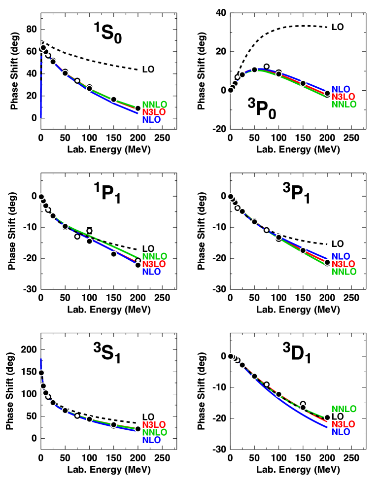
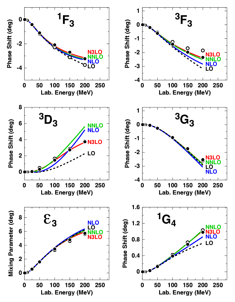
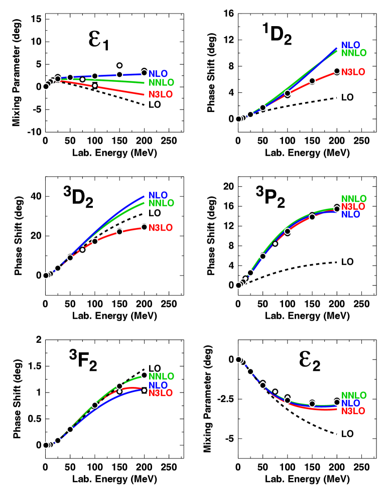
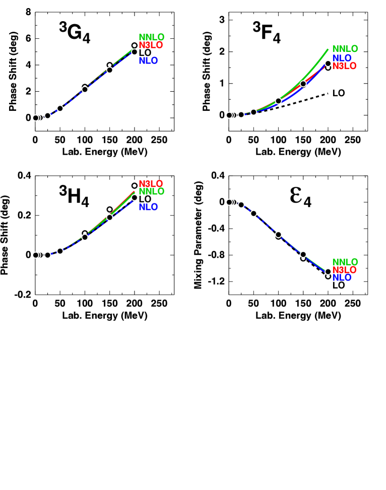
Figure 5: Chiral expansion of neutron-proton scattering as represented by the phase parameters for $J\leq 4$. Four orders ranging from LO to N³LO are shown as denoted. The cutoff combination $(R_{\pi},R_{\rm ct})=(1.0,0.70)$ fm is applied in all cases. The filled and open circles represent the results from the Nijmegen multi-energy $np$ phase-shift analysis Sto93 and the GWU single-energy $np$ analysis SP07 SP07 , respectively.

Table 3: $\chi^{2}/$datum for several energy intervals as obtained from the fit of the 2016 $NN$ database EMN17 by $NN$ potentials at various orders of chiral EFT applying the cutoff combination $(R_{\pi},R_{\rm ct})=(1.0,0.70)$ fm. Note that the $\chi^{2}$ is always minimized for the interval 0–190 MeV.

$T_{\rm lab}$ bin (MeV)	No. of data	LO	NLO	NNLO	N3LO
proton-proton
0–100	795	433	1.85	2.64	1.32
0–190	1206	363	4.60	7.84	1.33
0–290	2132	341	16.2	18.1	1.69
neutron-proton
0–100	1180	211	1.58	2.34	1.59
0–190	1697	157	15.0	10.2	1.53
0–290	2721	109	35.4	21.4	1.99
$pp$ plus $np$
0–100	1975	300	1.68	2.45	1.48
0–190	2903	243	10.7	9.23	1.45
0–290	4853	203	26.9	20.0	1.86

The free (fit) parameters of our theory are the coefficients of the contact terms presented in Sec. II.4. The other set of parameters involved in $NN$ potential construction are the $\pi N$ LECs. We apply the ones from the very accurate Roy-Steiner analysis of Ref. Hof15 given in Table 1. We use the central values and, thus, the $\pi N$ LECs are precisely fixed from the outset and no fit parameters.

Fitting proceeds in two steps. First we fit phase shifts, where the adjustment is done to the Nijmegen multi-energy analysis Sto93 , which we perceive as the most reliable one. In the second step, the potential predictions are confronted with the experimental $NN$ data—calculating the $\chi^{2}$ as follows.

The experimental data are broken up into groups (sets) of data, $A$, with $N_{A}$ data points and an experimental over-all normalization uncertainty $\Delta n_{A}^{exp}$. For datum $i$ of set $A$, $x^{exp}_{A,i}$ is the experimental value, $\Delta x^{exp}_{A,i}$ the experimental uncertainty, and $x^{mod}_{A,i}$ the model prediction. When fitting the data of group $A$ by a model (or a phase shift solution), the over-all normalization, $n_{A}^{mod}$, is floated and finally chosen such as to minimize the $\chi^{2}$ for this group. The $\chi^{2}$ is then calculated from Ber88

$$\chi^{2}=\sum_{A}\left\{\sum^{N_{A}}_{i=1}\left[\frac{n_{A}^{mod}\,\,x^{mod}_{A,i}\,-x^{exp}_{A,i}}{\Delta x^{exp}_{A,i}}\right]^{2}+\,\left[\frac{n_{A}^{mod}\,-1}{\Delta n_{A}^{exp}}\right]^{2}\right\}\;;$$ (55)

that is, the over-all normalization of a group is treated as an additional parameter. For groups of data without normalization uncertainty ($\Delta n_{A}^{exp}=0$), $n_{A}^{mod}=1$ is used and the second term on the r.h.s. of Eq. (55) is dropped. The total number of data is

$$N_{dat}=N_{obs}+N_{ne}$$ (56)

where $N_{obs}$ denotes the total number of measured data points (observables), i. e., $N_{obs}=\sum_{A}N_{A}$; and $N_{ne}$ is the number of experimental normalization uncertainties. We state results in terms of $\chi^{2}/N_{dat}\equiv\chi^{2}/$datum, where we use for the experimental $NN$ data the “2016 database” defined in Ref. EMN17 .

Each of the two steps described above, is done in two parts. In part one, we adjust the $pp$ potential, which fixes the $T=1$ partial waves (where $T$ denotes the total isospin of the two-nucleon system). In part two, the charge-dependence described in Sec. II.5 is applied to obtain the $np$ $T=1$ phase shifts from the $pp$ ones. The $np$ $T=0$ partial-waves are then pinned down by first fitting phase shifts and, after that, minimizing the $\chi^{2}$ in regard to the $np$ data. During this last step, we allowed for minor changes of the $T=1$ parameters (which also modifies the $pp$ potential) to obtain an even lower overall $\chi^{2}$. We always minimize the $\chi^{2}$ for the energy range 0-190 MeV laboratory energy ($T_{\rm lab}$). For more details on the $NN$ database and the fitting procedure, see Ref. EMN17 .

The $nn$ potential is obtained by starting from the $pp$ version, replacing the proton mass by the neutron mass in the kinetic energy, leaving out Coulomb, and adjusting the zeroth-order contacts such as to reproduce the empirical $nn$ ${}^{1}S_{0}$ scattering length of –18.95 fm Gon06 ; Che08 .

The contact LECs that result from our best fits at N³LO are tabulated in Appendix B.

Plots of the various components of the chiral potentials in comparison to more traditional potentials are shown and discussed in Appendix C.

The $\chi^{2}$/datum for the reproduction of the $NN$ data at various orders of chiral EFT are shown in Table 3 for different energy intervals below $T_{\rm lab}=290$ MeV. The most relevant energy interval is the one from 0–190 MeV, for which the $\chi^{2}$/datum is 10.7 at NLO and 9.2 at NNLO for the $pp$ plus $np$ data. Note that the number of $NN$ contact terms is the same for both orders, which may naively explain why there is essentially no change. However, for nonlocal momentum-space potentials EMN17 the $\chi^{2}$ at NNLO turns out to be substantially lower than at NLO, because of a large 2PE contribution at NNLO providing the proper intermediate-range attraction for the nuclear force. The fact that this is not happening for the present local potentials may have the following explanation: First note that our $\chi^{2}$ at NLO is already unusually low as compared to what nonlocal momentum-space potentials (cf., e.g., Ref. EMN17 ) generate at that order leaving not much room for improvement at NNLO. The unusually good results at NLO may be due to the fact that the iteration of a locally regularized 1PE creates a larger 2PE contribution than the iteration of a nonlocal one. After all, the reason why NLO is in general not doing well is a lack of a sizable 2PE contribution.

Finally, moving on to N³LO, 14 more contacts are added [Eq. (35)] that affect, in particular, the the ${}^{1}D_{2}$ and ${}^{3}D_{2}$ waves, which typically come out far too attractive at NLO and NNLO (Fig. 5). This improves the $\chi^{2}$/datum to 1.45 at N³LO, a respectable value.

All $np$ phase shifts up to $J=4$ and $T_{\rm lab}=200$ MeV are displayed in Fig. 5, which reflects what just has been said in the context of the the $\chi^{2}$. At this point, it is instructive to talk about the uncertainties of the phase shift predictions. As discussed in Sec. IV below, the truncation error creates the largest uncertainty, for which the simplest formula is given by Eq. (57). Following this prescription, the error at a certain order is the difference between the given order and the next higher one. For example, the uncertainties of our NNLO phase shifts are given by the differences between the (green) NNLO curves and the (red) N3LO curves in Fig. 5. For the uncertainty at N3LO, Eq. (58) has to be invoked. The factor $Q$ in this formula is, of course, energy dependent but, as a simple rule of thumb, one may assume $Q\approx 1/3$.

Table 4: Scattering lengths ($a$) and effective ranges ($r$) in units of fm as predicted by $NN$ potentials at various orders of chiral EFT applying the cutoff combination $(R_{\pi},R_{\rm ct})=(1.0,0.70)$ fm. ($a_{pp}^{C}$ and $r_{pp}^{C}$ refer to the $pp$ parameters in the presence of the Coulomb force. $a^{N}$ and $r^{N}$ denote parameters determined from the nuclear force only and with all electromagnetic effects omitted.) $a_{nn}^{N}$, and $a_{np}$ are fitted, all other quantities are predictions.

	LO	NLO	NNLO	N3LO	Empirical
${}^{1}S_{0}$
$a_{pp}^{C}$	–7.8161	–7.8134	–7.8147	–7.8136	–7.8196(26) Ber88
					–7.8149(29) SES83
$r_{pp}^{C}$	2.009	2.715	2.764	2.748	2.790(14) Ber88
					2.769(14) SES83
$a_{pp}^{N}$	—	–17.364	–17.466	–17.391	—
$r_{pp}^{N}$	—	2.788	2.834	2.818	—
$a_{nn}^{N}$	–18.950	–18.950	–18.950	–18.950	–18.95(40) Gon06 ; Che08
$r_{nn}^{N}$	1.985	2.761	2.807	2.790	2.86(10) Mal22
$a_{np}$	–23.738	–23.738	–23.738	–23.738	–23.740(20) Mac01
$r_{np}$	1.888	2.653	2.695	2.679	[2.77(5)] Mac01
${}^{3}S_{1}$
$a_{t}$	5.299	5.414	5.413	5.420	5.419(7) Mac01
$r_{t}$	1.586	1.750	1.747	1.756	1.753(8) Mac01

The low-energy scattering parameters, order by order for the cutoff combination $(R_{\pi},R_{\rm ct})=(1.0,0.70)$ fm, are shown in Table 4. For $nn$ and $np$, the effective range expansion without any electromagnetic interaction is used. In the case of $pp$ scattering, the quantities $a_{pp}^{C}$ and $r_{pp}^{C}$ are obtained by using the effective range expansion appropriate in the presence of the Coulomb force (cf. Appendix A4 of Ref. Mac01 ). Note that the empirical values for $a_{pp}^{C}$ and $r_{pp}^{C}$ in Table 4 were obtained by subtracting from the corresponding electromagnetic values the effects due to two-photon exchange and vacuum polarization. Thus, the comparison between theory and experiment for these two quantities is conducted correctly. $a_{nn}^{N}$, and $a_{np}$ are fitted, all other quantities are predictions. Note that the ${}^{3}S_{1}$ effective range parameters $a_{t}$ and $r_{t}$ are not fitted. But the deuteron binding energy is fitted and that essentially fixes $a_{t}$ and $r_{t}$.

III.2 Electromagnetic effects

The full scattering amplitude for $NN$ scattering consists of two parts: the strong-interactions (nuclear) amplitude plus the electromagnetic (em) amplitude. Following the way the Nijmegen partial-wave analysis was conducted Ber88 ; Sto93 ; SS90 , the em amplitude includes relativistic Coulomb, two-photon exchange, vacuum polarization, and magnetic moment (MM) interactions. The nuclear amplitude is parametrized in terms of the strong nuclear phase shifts which are to be calculated in the presence of the em interaction, i. e., with respect to em wave functions. In the case of $pp$ scattering, it is in general a good approximation to just use the phase shifts of the nuclear plus relativistic Coulomb interaction with respect to Coulomb wave functions. The exception are the ${}^{1}S_{0}$ $pp$ phase shifts below 30 MeV, where electromagnetic phase shifts are to be used, which are obtained by correcting the Coulomb phase shifts for the distorting effects from two-photon exchange, vacuum polarization, and MM interactions as calculated by the Nijmegen group Ber88 ; Sto95 . In the case of $np$ and $nn$ scattering, the phase shifts from the nuclear interaction with respect to Riccati-Bessel functions are applied. More technical details of our phase shift calculations can be found in Appendix A3 of Ref. Mac01 .

The $NN$ potentials constructed in this paper represent the strong nuclear interaction between two nucleons. Electromagnetic interactions are not provided, because they are well known and readily available elsewhere WSS95 . In applications of the potentials in the nuclear many-body problem, one would add at least the Coulomb interaction between protons. Other more subtle em interactions between protons, like, two-photon-exchange, vacuum polarization, and MM interactions, can also be added to our nuclear $pp$ potentials. However their effects are, in general, very small and, in fact, much smaller than the effects from off-shell differences between different strong nuclear potentials. Thus, in most applications, there is no significance to their inclusion.

A special word is called-for concerning our $np$ potentials. Following tradition Sto93 ; Sto94 ; Mac01 ; EMN17 ; RKE18 ; NAA13 , we fit the experimental ${}^{1}S_{0}$ $np$ scattering length, $a_{np}=-23.74$ fm (cf. Table 4), and the experimental deuteron binding energy, $B_{d}=2.22458$ MeV. This implies that we tacitly include the $np$ MM interaction in our strong interaction $np$ potentials. This is not unreasonable, because, e. g. in ${}^{1}S_{0}$, only a MM contact term with the range of the $\rho$ meson contributes, which is naturally absorbed by the contacts of the EFT potentials. Therefore, no em interactions must be added to our $np$ potentials.

The bottom line is that, in typical nuclear many-body calculations, all that needs to be added to our strong $NN$ potentials is the Coulomb force between protons (and nuclear three-nucleon forces).

III.3 The deuteron and triton

The evolution of the deuteron properties from LO to N³LO of chiral EFT are shown in Table 5. In all cases, we fit the deuteron binding energy ($B_{d}$) to its empirical value of 2.22458 MeV using the LO contact parameters. All other deuteron properties are predictions. Note, however, that the asymptotic $S$ state, $A_{S}$, and the ${}^{3}S_{1}$ effective range parameter, $r_{t}$, are related KMS84 ; MV84 ; STS95 and, furthermore, the $r_{t}$ is strongly correlated with $B_{d}$. Thus, the fact that, at NLO and up, $A_{S}$ falls essentially within the empirical range is no real freelance prediction. In contrast, the asymptotic $D/S$ state, $\eta$, is more versatile. While at LO, NLO, and NNLO, the predictions agree with experiment, the value at N³LO is low and outside the N³LO truncation error. This phenomenon is most likely related to the local character of the present potentials, since such underprediction is not happening with nonlocal potentials at N³LO (and N⁴LO) EMN17 . It represents an interesting topic for future investigations (see also the $\epsilon_{1}$ discussion, below).

At the bottom of Table 5, we also show the predictions for the triton binding as obtained in 34-channel charge-dependent Faddeev calculations using only 2NFs. The result is around 8.1 MeV at N³LO. This contribution from the 2NF will require only a moderate 3NF. The relatively low deuteron $D$-state probabilities ($\approx 4$% at N³LO) and the concomitant generous triton binding energy predictions are a reflection of the fact that our $NN$ potentials have a weaker tensor force than commonly used local position-space potentials. This can also be seen in the predictions for the $\epsilon_{1}$ mixing parameter that is a measure for the strength of the mixing of the ${}^{3}S_{1}$ and ${}^{3}D_{1}$ states due to the tensor force. Our predictions for $\epsilon_{1}$ at NNLO and N³LO are on the lower side for lab. energies above 100 MeV (Fig. 5). However, there is agreement with the GWU analysis SP07 at 100 MeV. Note that the average relative momentum in nuclear matter at normal density is equivalent to $T_{\rm lab}\approx 50$ MeV. Thus, the properties of $NN$ potentials for $T_{\rm lab}\raisebox{-1.29167pt}{\small$\ \stackrel{{\scriptstyle\textstyle<}}{{\sim}}$ }100$ MeV are the most important ones for nuclear structure applications. Moreover, the discrepancies between the Nijmegen Sto93 and the GWU SP07 analyses for $\epsilon_{1}$ may be seen as an indication that this parameter is not as well determined as the uncertainties quoted in the analyses suggest. The $\chi^{2}$/datum of our N³LO potential is 1.45, which is a typical value achieved in the GWU phase shift analyses. Furthermore, the $\chi^{2}$/datum (for the energy range 0–$\approx$200 MeV) for the well-established and highly appreciated N³LO potentials of Refs. Pia16 ; EMN17 ; RKE18 are 1.40, 1.35, and 1.50, respectively. The fact that our $\chi^{2}$/datum is the same as for the referenced potentials, while our $\epsilon_{1}$ differs, implies that our $\epsilon_{1}$ prediction is as consistent with the data as the alternatives and may simply be viewed as another valid phase shift analysis.

We finally note that the observation that a weak tensor force (low $P_{D}$) causes a low $\epsilon_{!}$ at intermediate energies is a typical feature of local $NN$ potentials. For nonlocal potentials there is not necessarily such a trend as the weak-tensor force potentials of Ref. EMN17 demonstrate.

Table 5: Two- and three-nucleon bound-state properties as predicted by $NN$ potentials at various orders of chiral EFT applying the cutoff combination $(R_{\pi},R_{\rm ct})=(1.0,0.70)$ fm. (Deuteron: Binding energy $B_{d}$, asymptotic $S$ state $A_{S}$, asymptotic $D/S$ state $\eta$, quadrupole moment $Q$, $D$-state probability $P_{D}$; the prediction for $Q$ is without meson-exchange current contributions and relativistic corrections. Triton: Binding energy $B_{t}$.) $B_{d}$ is fitted, all other quantities are predictions.

	LO	NLO	NNLO	N3LO	Empiricala
Deuteron
$B_{d}$ (MeV)	2.22458	2.22458	2.22458	2.22458	2.224575(9)
$A_{S}$ (fm-1/2)	0.8613	0.8833	0.8836	0.8852	0.8846(9)
$\eta$	0.0254	0.0259	0.0252	0.0242	0.0256(4)
$Q$ (fm2)	0.264	0.284	0.274	0.260	0.2859(3)
$P_{D}$ (%)	5.08	5.67	5.02	4.03	—
Triton
$B_{t}$ (MeV)	11.88	7.87	7.98	8.09	8.48

^aSee Table XVIII of Ref. Mac01 for references.

III.4 Cutoff variations

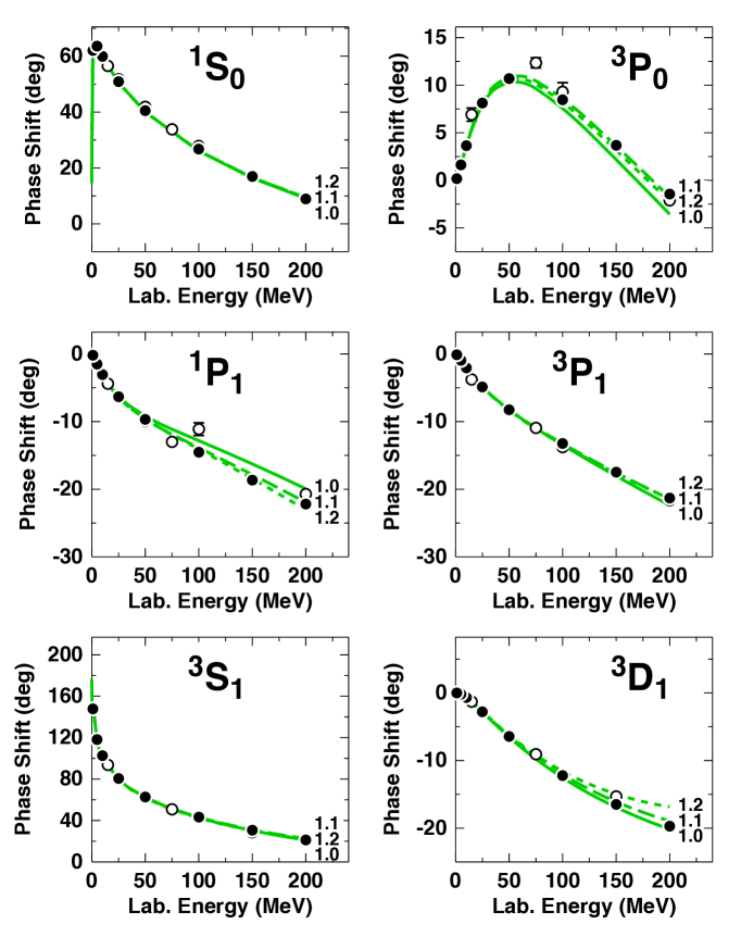
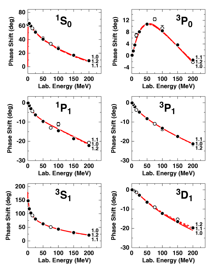
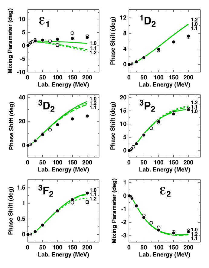
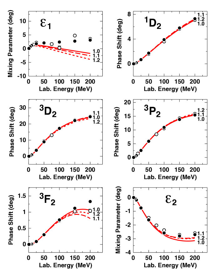
Figure 6: Cutoff variations of the $np$ phase shifts at NNLO (left side, green lines) and N³LO (right side, red lines). Solid, dashed, and dotted lines represent the results obtained with the cutoff combinations $(R_{\pi},R_{\rm ct})$ = (1.0, 0.70) fm, (1.1, 0.72) fm, and (1.2, 0.75) fm, respectively, as also indicated by the curve labels which state the $R_{\pi}$ value. Filled and open circles as in Fig. 5.

Table 6: $\chi^{2}$/datum for the fit of the $pp$ plus $np$ data up to 100 MeV and two- and three-nucleon bound-state properties as produced by $NN$ potentials at NNLO and N³LO with the cutoff combinations $(R_{\pi},R_{\rm ct})=(1.2,0.75)$ fm, $(1.1,0.72)$ fm, and $(1.0,0.70)$ fm. In the column headings, we use the $R_{\pi}$ value to identify the different cases. For some of the notation, see Table 5, where also empirical information on the deuteron and triton can be found.

	NNLO			N3LO
	$R_{\pi}=1.2$ fm	$R_{\pi}=1.1$ fm	$R_{\pi}=1.0$ fm	$R_{\pi}=1.2$ fm	$R_{\pi}=1.1$ fm	$R_{\pi}=1.0$ fm
$\chi^{2}$/datum $pp$ & $np$
0–100 MeV (1975 data)	2.75	2.39	2.45	1.75	1.56	1.48
Deuteron
$B_{d}$ (MeV)	2.22458	2.22458	2.22458	2.22458	2.22458	2.22458
$A_{S}$ (fm-1/2)	0.8862	0.8835	0.8836	0.8842	0.8851	0.8852
$\eta$	0.0244	0.0246	0.0252	0.0234	0.0239	0.0242
$Q$ (fm2)	0.263	0.265	0.274	0.248	0.255	0.260
$P_{D}$ (%)	3.98	4.27	5.02	3.22	3.65	4.03
Triton
$B_{t}$ (MeV)	8.31	8.25	7.98	8.40	8.18	8.09

As noted before, besides the cutoff combination $(R_{\pi},R_{\rm ct})=(1.0,0.70)$ fm, we have also constructed potentials with the combinations (1.1, 0.72) fm, and (1.2, 0.75) fm, to allow for systematic studies of the cutoff dependence. In Fig. 6, we display the variations of the $np$ phase shifts for different cutoffs at NNLO (left half of figure, green curves) and at N³LO (right half of figure, red curves). Fig. 6 demonstrates nicely how cutoff dependence diminishes with increasing order—a reasonable trend. Another point that is evident from this figure is that (1.2, 0.75) fm should be considered as an upper limit for cutoffs, because obviously cutoff artifacts start showing up.

In Table 6, we show the cutoff dependence for three selected aspects that are of great interest: the $\chi^{2}$ for the fit of the $NN$ data below 100 MeV, the deuteron properties, and the triton binding energy. The $\chi^{2}$ does not change substantially as a function of cutoff. Thus, we can make the interesting observation that the reproduction of $NN$ observables is not much affected by the cutoff variations. However, the $D$-state probability of the deuteron, $P_{D}$, which is not an observable, changes substantially as a function of cutoff. As discussed, $P_{D}$ is intimately related to the strength of the tensor force of a potential and so are the binding energies of few-body systems. In particular, the cutoff combination $(R_{\pi},R_{\rm ct})=(1.1,0.72)$ fm and (1.2, 0.75) fm at NNLO as well as N³LO generate the substantial triton binding energies between 8.20 and 8.40 MeV and, therefore, differ significantly from other local position-space potentials that are commonly in use. On these grounds one can expect that results for light and intermediate-mass nuclei may differ considerably when applying our potentials in ab initio calculations. It will be interesting to see if this may solve some of the problems that some ab initio calculations with local potentials are currently beset with.

IV Uncertainty quantifications

In ab initio calculations applying chiral two- and many-body forces, major sources of uncertainties are FPW15 :

1. Experimental errors of the input $NN$ data that the 2NFs are based upon and the input few-nucleon data to which the 3NFs are adjusted.

2. Uncertainties in the Hamiltonian due to

   1. uncertainties in the determination of the $NN$ and $3N$ contact LECs,

   2. uncertainties in the $\pi N$ LECs,

   3. regulator dependence,

   4. EFT truncation error.

3. Uncertainties associated with the few- and many-body methods applied.

The experimental errors in the $NN$ scattering and deuteron data propagate into the $NN$ potentials that are adjusted to reproduce those data. To systematically investigate this error propagation, the Granada group has constructed smooth local potentials PAA14 , the parameters of which carry the uncertainties implied by the errors in the $NN$ data. Applying 205 Monte Carlo samples of these potentials, they find an uncertainty of 15 keV for the triton binding energy Per14 . In a more recent study Per15 , in which only 33 Monte Carlo samples were used, the Granada group reproduced the uncertainty of 15 keV for the triton binding energy and, in addition, determined the uncertainty for the ⁴He binding energy to be 55 keV. The conclusion is that the statistical error propagation from the $NN$ input data to the binding energies of light nuclei is negligible as compared to uncertainties from other sources (discussed below). Thus, this source of error can be safely neglected at this time. Furthermore, we need to consider the propagation of experimental errors from the experimental few-nucleon data that the 3NF contact terms are fitted to. Also this will be negligible as long as the 3NFs are adjusted to data with very small experimental errors; for example the empirical binding energy of the triton is $8.481795\pm 0.000002$ MeV, which will definitely lead to negligible propagation.

Now turning to the Hamiltonian, we have to, first, account for uncertainties in the $NN$ and $3N$ LECs due to the way they are fixed. Based upon our experiences from Ref. Mar13 and the fact that chiral EFT is a low-energy expansion, we have fitted the $NN$ contact LECs to the $NN$ data below 100 MeV at LO and NLO and below 190 MeV at NNLO and N³LO. One could think of choosing these fit-intervals slightly different and a systematic investigation of the impact of such variation on the $NN$ LECs is still outstanding. However, we do not anticipate that large uncertainties would emerge from this source of error.

The story is different for the 3NF contact LECs, since several, very different procedures are in use for how to fix them. The 3NF at NNLO has two free parameters (known as the $c_{D}$ and $c_{E}$ parameters). To fix them, two data are needed. In most procedures, one of them is the triton binding energy. For the second datum, the following choices have been made: the $nd$ doublet scattering length ${}^{2}a_{nd}$ Epe02 , the binding energy of ⁴He Nog06 , the point charge radius radius of ⁴He Heb11 , the Gamow-Teller matrix element of tritium $\beta$-decay GP06 ; GQN09 ; Mar12 . Alternatively, the $c_{D}$ and $c_{E}$ parameters have also been pinned down by just an optimal over-all fit of the properties of light nuclei Nav07a . 3NF contact LECs determined by different procedures will lead to different predictions for the observables that were not involved in the fitting procedure. The differences in those results establish the uncertainty. Specifically, it would be of interest to investigate the differences that occur for the properties of intermediate-mass nuclei and nuclear matter when 3NF LECs fixed by different protocols are applied.

The uncertainty in the $\pi N$ LECs used to be a large source of uncertainty, in particular, for predictions for many-body systems Kru13 ; DHS16 ; Dri16 . With the new, high-precision determination of the $\pi N$ LECs in the Roy-Steiner equations analysis Hof15 (cf. Table 1) this large uncertainty is essentially eliminated, which is great progress, since it substantially reduces the error budget. We have varied the $\pi N$ LECs within the errors given in Table 1 and find that the changes caused by these variations can easily be compensated by small readjustments of the $NN$ LECs resulting in essentially identical phase shifts and $\chi^{2}$ for the fit of the data. Thus, this source of error is essentially negligible. The $\pi N$ LECs also appear in the 3NFs, which also include contacts that can be used for readjustment. Future calculations of finite nuclei and nuclear matter should investigate what residual changes remain after such readjustment (that would represent the uncertainty). We expect this to be small.

The choice of the regulator function and its cutoff parameter create uncertainty. Originally, cutoff variations were perceived as a demonstration of the uncertainty at a given order (equivalent to the truncation error). However, in various investigations Sam15 ; EKM15 it has been demonstrated that this is not correct and that cutoff variations, in general, underestimate this uncertainty. Therefore, the truncation error is better determined by sticking literally to what ‘truncation error’ means, namely, the error due to omitting the contributions from orders beyond the given order $\nu$. The largest such contribution is the one of order $(\nu+1)$, which one may, therefore, consider as representative for the magnitude of what is left out. This suggests that the truncation error at order $\nu$ can reasonably be defined as

$$\Delta X_{\nu}(p)=|X_{\nu}(p)-X_{\nu+1}(p)|\,,$$ (57)

where $X_{\nu}(p)$ denotes the prediction for observable $X$ at order $\nu$ and momentum $p$. If $X_{\nu+1}$ is not available, then one may use,

$$\Delta X_{\nu}(p)=|X_{\nu-1}(p)-X_{\nu}(p)|Q\,,$$ (58)

with the expansion parameter $Q$ chosen as

$$Q=\max\left\{\frac{m_{\pi}}{\Lambda_{b}},\;\frac{p}{\Lambda_{b}}\right\}\,,$$ (59)

where $p$ is the characteristic center-of-mass (cms) momentum scale and $\Lambda_{b}$ the breakdown scale.

Alternatively, one may also apply the more elaborate scheme suggested in Ref. EKM15 where the truncation error at, e.g., N³LO is calculated in the following way:

$$\Delta X_{\rm N^{3}LO}(p) = \max\left\{Q^{5}\times\left|X_{\rm LO}(p)\right|,\;\;Q^{3}\times\left|X_{\rm LO}(p)-X_{\rm NLO}(p)\right|,\;\;Q^{2}\times\left|X_{\rm NLO}(p)-X_{\rm NNLO}(p)\right|,\;\;\right.$$ (61)

$$\left.Q\times\left|X_{\rm NNLO}(p)-X_{\rm N^{3}LO}(p)\right|\right\}\,,$$

with $X_{\rm N^{3}LO}(p)$ denoting the N³LO prediction for observable $X(p)$, etc..

Note that one should not add up (in quadrature) the uncertainties due to regulator dependence and the truncation error, because they are not independent. In fact, it is appropriate to leave out the uncertainty due to regulator dependence entirely and just focus on the truncation error EKM15 . The latter should be estimated using the same cutoff in all orders considered.

Finally, the last uncertainty to be taken into account is the uncertainty in the few- and many-body methods applied in the ab initio calculation. This source of error has nothing to do with EFT. Few-body problems are nowadays exactly solvable such that the error is negligible in those cases. For heavier nuclei and nuclear matter, there are definitely uncertainties no matter what method is used. These uncertainties need to be estimated by the practitioners of those methods. But with the improvements of algorithms and the increase of computing power these errors are decreasing.

The conclusion is that the most substantial uncertainty is represented by the truncation error. This is the dominant source of (systematic) error that should be carefully estimated for any calculation applying chiral 2NFs and 3NFs up to a given order.

V Summary and Conclusions

We have constructed local, position-space chiral $NN$ potentials through four orders of chiral EFT ranging from LO to N³LO. The construction may be perceived as consistent, because the same power counting scheme as well as the same cutoff procedures are applied in all orders. Moreover, the long-range parts of these potentials are fixed by the very accurate $\pi N$ LECs as determined in the Roy-Steiner equations analysis of Ref. Hof15 . In fact, the uncertainties of these LECs are so small that a variation within the errors leads to effects that are essentially negligible at the current level of precision. Another aspect that has to do with precision is that, at least at the highest order (N³LO), the $NN$ data below 190 MeV laboratory energy are reproduced with the respectable $\chi^{2}$/datum of 1.45.

The $NN$ potentials presented in this paper may serve as a solid basis for systematic ab initio calculations of nuclear structure and reactions that allow for a comprehensive error analysis. In particular, the order by order development of the potentials will make possible a reliable determination of the truncation error at each order.

Our new family of local position-space potentials differs from the already available potentials of this kind Gez14 ; Pia15 ; Pia16 by a weaker tensor force as reflected in relatively low $D$-state probabilities of the deuteron ($P_{D}\raisebox{-1.29167pt}{\small$\ \stackrel{{\scriptstyle\textstyle<}}{{\sim}}$ }4.0$ % for our N³LO potentials) and predictions for the triton binding energy above 8.00 MeV (from two-body forces alone). As a consequence, our potentials will also lead to different predictions when applied to light and intermediate-mass nuclei in ab initio calculations note2 . It will be interesting to see if this will help solving some of the outstanding problems in microscopic nuclear structure.

Appendix A The long-range $NN$ potential

For each order, we will state, first, the momentum-space functions and then the corresponding position-space potentials as obtained by Fourier transform. Note that all long-range potentials are local.

In momentum space, we use the following decomposition of the long-range potential,

$$V_{\pi}({\vec{p}}~{}^{\prime},\vec{p}) = \,\>\>\>\>\,V_{C}(q)\>\,+\bm{\tau}_{1}\cdot\bm{\tau}_{2}\,W_{C}(q)$$ (62)

$$+\left[\,V_{S}(q)\>\,+\bm{\tau}_{1}\cdot\bm{\tau}_{2}\,W_{S}(q)\,\>\,\right]\,\vec{\sigma}_{1}\cdot\vec{\sigma}_{2}$$

$$+\left[\,V_{T}(q)\>\,+\bm{\tau}_{1}\cdot\bm{\tau}_{2}\,W_{T}(q)\,\>\,\right]\,\vec{\sigma}_{1}\cdot\vec{q}\,\,\vec{\sigma}_{2}\cdot\vec{q}$$

$$+\left[\,V_{LS}(q)+\bm{\tau}_{1}\cdot\bm{\tau}_{2}\,W_{LS}(q)\right]\left(-i\vec{S}\cdot(\vec{q}\times\vec{k})\,\right)\,.$$

For notation, see Sec. II.4. The position-space potential is represented as follows:

$$\widetilde{V}_{\pi}(\vec{r}) = \,\,\>\>\>\>\,\widetilde{V}_{C}(r)\>\,+\bm{\tau}_{1}\cdot\bm{\tau}_{2}\,\widetilde{W}_{C}(r)$$ (63)

$$+\left[\,\widetilde{V}_{S}(r)\>\,+\bm{\tau}_{1}\cdot\bm{\tau}_{2}\,\widetilde{W}_{S}(r)\,\>\,\right]\,\vec{\sigma}_{1}\cdot\vec{\sigma}_{2}$$

$$+\left[\,\widetilde{V}_{T}(r)\>\,+\bm{\tau}_{1}\cdot\bm{\tau}_{2}\,\widetilde{W}_{T}(r)\,\>\,\right]\,S_{12}(\hat{r})$$

$$+\left[\,\widetilde{V}_{LS}(r)+\bm{\tau}_{1}\cdot\bm{\tau}_{2}\,\widetilde{W}_{LS}(r)\right]\vec{L}\cdot\vec{S}\,,$$

where the operator for total orbital angular momentum is denoted by $\vec{L}$.

The 2PE potentials in spectral representation are given in momentum space by

$$V_{C,S}(q) = -\frac{2q^{6}}{\pi}\int_{2m_{\pi}}^{\infty}d\mu\frac{{\rm Im}V_{C,S}(i\mu)}{\mu^{5}(\mu^{2}+q^{2})}\,,$$

$$V_{T,LS}(q) = \frac{2q^{4}}{\pi}\int_{2m_{\pi}}^{\infty}d\mu\frac{{\rm Im}V_{T,LS}(i\mu)}{\mu^{3}(\mu^{2}+q^{2})}\,,$$ (64)

and similarly for $W_{C,S,T,LS}$. Their Fourier transforms are

$$\widetilde{V}_{C}(r) = \frac{1}{2\pi^{2}r}\int_{2m_{\pi}}^{\infty}d\mu\mu e^{-\mu r}{\rm Im}V_{C}(i\mu)\,,$$

$$\widetilde{V}_{S}(r) = -\frac{1}{6\pi^{2}r}\int_{2m_{\pi}}^{\infty}d\mu\mu e^{-\mu r}\left[\mu^{2}{\rm Im}V_{T}(i\mu)-3{\rm Im}V_{S}(i\mu)\right]\,,$$

$$\widetilde{V}_{T}(r) = -\frac{1}{6\pi^{2}r^{3}}\int_{2m_{\pi}}^{\infty}d\mu\mu e^{-\mu r}(3+3\mu r+\mu^{2}r^{2}){\rm Im}V_{T}(i\mu)\,,$$

$$\widetilde{V}_{LS}(r) = \frac{1}{2\pi^{2}r^{3}}\int_{2m_{\pi}}^{\infty}d\mu\mu e^{-\mu r}(1+\mu r){\rm Im}V_{LS}(i\mu)\,,$$ (65)

and similarly for $\widetilde{W}_{C,S,T,LS}$.

A.1 Leading order

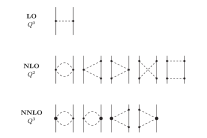
Figure 7: LO, NLO, and NNLO pion-exchange contributions to the $NN$ interaction. Notation as in Fig. 1.

At leading order, only 1PE contributes to the long range, cf. Fig. 7. The charge-independent 1PE is given in momentum space by

$$W_{T}(q)=-\frac{g_{A}^{2}}{4f_{\pi}^{2}}\>\frac{1}{q^{2}+m_{\pi}^{2}}\,,$$ (66)

where $g_{A}$, $f_{\pi}$, and $m_{\pi}$ denote the axial-vector coupling constant, pion-decay constant, and the pion mass, respectively. See Table 2 for their values. Fourier transform yields:

$$\widetilde{W}_{S}(r) = \frac{g_{A}^{2}m_{\pi}^{2}}{48\pi f_{\pi}^{2}}\;\frac{e^{-x}}{r}\,,$$ (67)

$$\widetilde{W}_{T}(r) = \frac{g_{A}^{2}}{48\pi f_{\pi}^{2}}\;\frac{e^{-x}}{r^{3}}(3+3x+x^{2})\,,$$ (68)

with $x=m_{\pi}r$.

For the $NN$ potentials constructed in this paper, we take the charge-dependence of the 1PE due to pion-mass splitting into account. For this, we define:

$$\widetilde{V}_{S}(m_{\pi}) = \frac{g_{A}^{2}m_{\pi}^{2}}{48\pi f_{\pi}^{2}}\;\frac{e^{-x}}{r}\,,$$ (69)

$$\widetilde{V}_{T}(m_{\pi}) = \frac{g_{A}^{2}}{48\pi f_{\pi}^{2}}\;\frac{e^{-x}}{r^{3}}(3+3x+x^{2})\,.$$ (70)

The proton-proton ($pp$) and neutron-neutron ($nn$) potentials are then given by:

$$\widetilde{V}_{S}^{(pp)}(r) = \widetilde{V}_{S}^{(nn)}(r)=\widetilde{V}_{S}(m_{\pi^{0}})\,,$$ (71)

$$\widetilde{V}_{T}^{(pp)}(r) = \widetilde{V}_{T}^{(nn)}(r)=\widetilde{V}_{T}(m_{\pi^{0}})\,,$$ (72)

and the neutron-proton ($np$) potentials are:

$$\widetilde{V}_{S}^{(np)}(r) = -\widetilde{V}_{S}(m_{\pi^{0}})+(-1)^{T+1}\,2\,\widetilde{V}_{S}(m_{\pi^{\pm}})\,,$$ (73)

$$\widetilde{V}_{T}^{(np)}(r) = -\widetilde{V}_{T}(m_{\pi^{0}})+(-1)^{T+1}\,2\,\widetilde{V}_{T}(m_{\pi^{\pm}})\,,$$ (74)

where $T=0,1$ denotes the total isospin of the two-nucleon system. See Table 2 for the precise values of the pion masses. Formally speaking, the charge-dependence of the 1PE exchange is of order NLO ME11 , but we include it also at leading order to make the comparison with the (charge-dependent) phase-shift analyses meaningful.

Alternatively, the charge-dependent 1PE can also be stated in terms of a “charge-independent” 1PE,

$$\widetilde{W}_{S}^{\rm CI}(r) = \frac{1}{3}\left[\widetilde{V}_{S}(m_{\pi^{0}})+2\,\widetilde{V}_{S}(m_{\pi^{\pm}})\right]\,,$$ (75)

$$\widetilde{W}_{T}^{\rm CI}(r) = \frac{1}{3}\left[\widetilde{V}_{T}(m_{\pi^{0}})+2\,\widetilde{V}_{T}(m_{\pi^{\pm}})\right]\,,$$ (76)

plus charge-dependent contributions given by,

$$\widetilde{V}^{\rm CD}(r) = \frac{1}{3}\left[\widetilde{V}_{S}(m_{\pi^{0}})-\widetilde{V}_{S}(m_{\pi^{\pm}})\right]\vec{\sigma}_{1}\cdot\vec{\sigma}_{2}\,T_{12}\,,$$ (77)

$$+ \frac{1}{3}\left[\widetilde{V}_{T}(m_{\pi^{0}})-\widetilde{V}_{T}(m_{\pi^{\pm}})\right]S_{12}\,T_{12}\,,$$ (78)

with the isotensor operator $T_{12}$ defined in Eq. (21).

A.2 Next-to-leading order

The 2PE $NN$ diagrams that occur at NLO (cf. Fig. 7) contribute—in momentum space— in the following way KBW97 :

$$W_{C}(q) = {L(q)\over 384\pi^{2}f_{\pi}^{4}}\left[4m_{\pi}^{2}(1+4g_{A}^{2}-5g_{A}^{4})+q^{2}(1+10g_{A}^{2}-23g_{A}^{4})-{48g_{A}^{4}m_{\pi}^{4}\over w^{2}}\right]\,,$$ (79)

$$V_{T}(q) = -{1\over q^{2}}V_{S}(q)\;=\;-{3g_{A}^{4}\over 64\pi^{2}f_{\pi}^{4}}L(q)\,,$$ (80)

with the logarithmic loop function

$$L(q)={w\over q}\ln{\frac{w+q}{2m_{\pi}}}\,$$ (81)

and $w=\sqrt{4m_{\pi}^{2}+q^{2}}$. Note that we apply dimensional renormalization for all loop diagrams. Moreover, in all 2PE contributions, we use the average pion-mass, i. e., $m_{\pi}=\bar{m}_{\pi}$ (cf. Table 2).

These expressions imply the spectral functions

$${\rm Im}W_{C}(i\mu) = -{1\over 768\pi f_{\pi}^{4}}\frac{\sqrt{\mu^{2}-4m_{\pi}^{2}}}{\mu}\left[4m_{\pi}^{2}(1+4g_{A}^{2}-5g_{A}^{4})-\mu^{2}(1+10g_{A}^{2}-23g_{A}^{4})-{48g_{A}^{4}m_{\pi}^{4}\over 4m_{\pi}^{2}-\mu^{2}}\right]\,,$$ (82)

$${\rm Im}V_{T}(i\mu) = {1\over\mu^{2}}{\rm Im}V_{S}(i\mu)\;=\;{3g_{A}^{4}\over 128\pi f_{\pi}^{4}}\frac{\sqrt{\mu^{2}-4m_{\pi}^{2}}}{\mu}\,.$$ (83)

Via Fourier transform, Eq. (65), the equivalent position-space potentials are:

$$\widetilde{W}_{C}(r) = \frac{m_{\pi}}{128\pi^{3}f_{\pi}^{4}}\frac{1}{r^{4}}\Bigl{\{}\left[1+2g_{A}^{2}(5+2x^{2})-g_{A}^{4}(23+12x^{2})\right]K_{1}(2x)$$ (84)

$$+x\left[1+10g_{A}^{2}-g_{A}^{4}(23+4x^{2})\right]K_{0}(2x)\Bigl{\}}\,,$$

$$\widetilde{V}_{S}(r) = \frac{g_{A}^{4}m_{\pi}}{32\pi^{3}f_{\pi}^{4}}\frac{1}{r^{4}}\left[3xK_{0}(2x)+(3+2x^{2})K_{1}(2x)\right]\,,$$ (85)

$$\widetilde{V}_{T}(r) = -\frac{g_{A}^{4}m_{\pi}}{128\pi^{3}f_{\pi}^{4}}\frac{1}{r^{4}}\left[12xK_{0}(2x)+(15+4x^{2})K_{1}(2x)\right]\,,$$ (86)

where $K_{0}$ and $K_{1}$ denote the modified Bessel functions.

A.3 Next-to-next-to-leading order

The 2PE NNLO contribution (cf. Fig. 7) is given by KBW97 :

$$V_{C} = {3g_{A}^{2}\over 16\pi f_{\pi}^{4}}\left[2m_{\pi}^{2}(c_{3}-2c_{1})+c_{3}q^{2}\right](2m_{\pi}^{2}+q^{2})A(q)\,,$$ (87)

$$W_{T} = -{1\over q^{2}}W_{S}=-{g_{A}^{2}\over 32\pi f_{\pi}^{4}}c_{4}w^{2}A(q)\,,$$ (88)

with the loop function

$$A(q)={1\over 2q}\arctan{q\over 2m_{\pi}}\,.$$ (89)

The associated spectral functions are

$${\rm Im}V_{C}(i\mu) = {3g_{A}^{2}\over 64\mu f_{\pi}^{4}}\left[2m_{\pi}^{2}(c_{3}-2c_{1})-c_{3}\mu^{2}\right](2m_{\pi}^{2}-\mu^{2})\,,$$ (90)

$${\rm Im}W_{T}(i\mu) = {1\over\mu^{2}}{\rm Im}W_{S}(i\mu)=-{g_{A}^{2}\over 128\mu f_{\pi}^{4}}c_{4}(4m_{\pi}^{2}-\mu^{2})\,;$$ (91)

which, by way of Eq. (65), yield the position-space expressions

$$\widetilde{V}_{C}(r) = \frac{3g_{A}^{2}}{32\pi^{2}f_{\pi}^{4}}\frac{e^{-2x}}{r^{6}}\left[2c_{1}x^{2}(1+x)^{2}+c_{3}(6+12x+10x^{2}+4x^{3}+x^{4})\right]\,,$$ (92)

$$\widetilde{W}_{S}(r) = \frac{g_{A}^{2}}{48\pi^{2}f_{\pi}^{4}}\frac{e^{-2x}}{r^{6}}c_{4}(1+x)(3+3x+2x^{2})\,,$$ (93)

$$\widetilde{W}_{T}(r) = -\frac{g_{A}^{2}}{48\pi^{2}f_{\pi}^{4}}\frac{e^{-2x}}{r^{6}}c_{4}(1+x)(3+3x+x^{2})\,.$$ (94)

A.4 Next-to-next-to-next-to-leading order

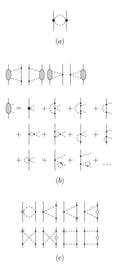
Figure 8: Two-pion exchange contributions at N³LO with (a) the N³LO football diagram, (b) the leading 2PE two-loop contributions, and (c) the leading relativistic corrections. Basic notation as in Fig. 1. The shaded disc stands for all one-loop $\pi N$ graphs as illustrated. Open circles are relativistic $1/M_{N}$ corrections.

A.4.1 Football diagram at N³LO

The N³LO football diagram, Fig. 8(a), generates Kai01a :

Momentum-space potentials:

$$V_{C}(q) = \frac{3\,L(q)}{16\pi^{2}f_{\pi}^{4}}\bigg{[}\bigg{(}\frac{c_{2}}{6}w^{2}+c_{3}(2m_{\pi}^{2}+q^{2})-4c_{1}m_{\pi}^{2}\bigg{)}^{2}+\frac{c_{2}^{2}}{45}w^{4}\bigg{]}\,,$$ (95)

$$W_{T}(q) = -\frac{1}{q^{2}}W_{S}(q)=\frac{c_{4}^{2}\,w^{2}\,L(q)}{96\,\pi^{2}f_{\pi}^{4}}\,.$$ (96)

Spectral functions:

$${\rm Im}V_{C}(i\mu) = -\frac{3}{32\pi f_{\pi}^{4}}\frac{\sqrt{\mu^{2}-4m_{\pi}^{2}}}{\mu}\bigg{[}\bigg{(}\frac{c_{2}}{6}(4m_{\pi}^{2}-\mu^{2})+c_{3}(2m_{\pi}^{2}-\mu^{2})-4c_{1}m_{\pi}^{2}\bigg{)}^{2}$$ (97)

$$+\frac{c_{2}^{2}}{45}(4m_{\pi}^{2}-\mu^{2})^{2}\bigg{]}\,,$$

$${\rm Im}W_{T}(i\mu) = \frac{1}{\mu^{2}}{\rm Im}W_{S}(i\mu)=\frac{c_{4}^{2}}{192\pi f_{\pi}^{4}}\frac{(\mu^{2}-4m_{\pi}^{2})^{3/2}}{\mu}\,.$$ (98)

Position-space potentials:

$$\widetilde{V}_{C}(r) = -\frac{3m_{\pi}^{7}}{32\pi^{3}f_{\pi}^{4}}\frac{1}{x^{5}}\bigg{[}\left(3c_{2}^{2}+20c_{2}c_{3}+60c_{3}^{2}+4(2c_{1}+c_{3})^{2}x^{2}\right)xK_{1}(2x)$$ (99)

$$+2\left(3c_{2}^{2}+20c_{2}c_{3}+60c_{3}^{2}+2(2c_{1}+c_{3})(c_{2}+6c_{3})x^{2}\right)K_{2}(2x)\bigg{]}\,,$$

$$\widetilde{W}_{S}(r) = \frac{c_{4}^{2}m_{\pi}^{7}}{24\pi^{3}f_{\pi}^{4}}\frac{1}{x^{4}}\bigg{[}2xK_{2}(2x)+5K_{3}(2x)\bigg{]}\,,$$ (100)

$$\widetilde{W}_{T}(r) = -\frac{c_{4}^{2}m_{\pi}^{7}}{96\pi^{3}f_{\pi}^{4}}\frac{1}{x^{5}}\bigg{[}(3+4x^{2})K_{2}(2x)+16xK_{3}(2x)\bigg{]}\,,$$ (101)

where $K_{2}(z)=K_{0}(z)+\frac{2}{z}K_{1}(z)$ and $K_{3}(z)=K_{1}(z)+\frac{4}{z}K_{2}(z)=\frac{4}{z}K_{0}(z)+(\frac{8}{z^{2}}+1)K_{1}(z)$.

A.4.2 Leading 2PE two-loop diagrams

The leading-order $2\pi$-exchange two-loop diagrams are shown in Fig. 8(b). The various contributions are Kai01a :

Isoscalar central potential:

Spectral functions:

$${\rm Im}V_{C}^{(a)}(i\mu) = -\frac{3g_{A}^{4}(\mu^{2}-2m_{\pi}^{2})}{\pi\mu(4f_{\pi})^{6}}\bigg{\{}(m_{\pi}^{2}-2\mu^{2})2m_{\pi}+4g_{A}^{2}m_{\pi}(2m_{\pi}^{2}-\mu^{2})\bigg{\}}\,,$$ (102)

$${\rm Im}V_{C}^{(b)}(i\mu) = -\frac{3g_{A}^{4}(\mu^{2}-2m_{\pi}^{2})}{\pi\mu(4f_{\pi})^{6}}(m_{\pi}^{2}-2\mu^{2})\frac{2m_{\pi}^{2}-\mu^{2}}{2\mu}\ln\frac{\mu+2m_{\pi}}{\mu-2m_{\pi}}\,.$$ (103)

Position-space potentials:

$$\widetilde{V}_{C}^{(a)}(r) = \frac{3m_{\pi}^{7}g_{A}^{4}}{2048\pi^{3}f_{\pi}^{6}}\frac{e^{-2x}}{x^{6}}\bigg{\{}24+48x+43x^{2}+22x^{3}+7x^{4}$$ (104)

$$+4g_{A}^{2}(6+12x+10x^{2}+4x^{3}+x^{4})\bigg{\}}\,,$$

$$\widetilde{V}_{C}^{(b)}(r) = -\frac{3m_{\pi}^{7}g_{A}^{4}}{8192\pi^{3}f_{\pi}^{6}}\frac{e^{-2x}}{x^{7}}\bigg{\{}(120+240x+213x^{2}+106x^{3}+32x^{4}+8x^{5})(\ln(4x)+\gamma_{E})$$ (105)

$$-(120-240x+213x^{2}-106x^{3}+32x^{4}-8x^{5})e^{4x}{\rm Ei}(-4x)$$

$$-4x(96+72x+38x^{2}+7x^{3})\bigg{\}}$$

$$+\frac{3m_{\pi}^{7}g_{A}^{4}}{4096\pi^{3}f_{\pi}^{6}}\frac{\bar{I}_{-1}(2x)}{x}\,,$$

where ${\rm Ei}(-z)$ denotes the exponential integral function defined by

$${\rm Ei}(-z)=-\int^{\infty}_{z}dt\,\frac{e^{-t}}{t}\,,$$ (106)

and

$$\bar{I}_{-1}(z)=\int_{1}^{\infty}dt\frac{e^{-zt}}{t}\ln\bigg{(}\frac{t+1}{t-1}\bigg{)}\,.$$ (107)

The double precision value for Euler’s constant is $\gamma_{E}=0.5772156649015329$.


Isovector central potential:

Spectral functions:

$${\rm Im}W_{C}^{(a)}(i\mu) = -\frac{2\kappa}{3\mu(8\pi f_{\pi}^{2})^{3}}\int_{0}^{1}dz\left[g_{A}^{2}(2m_{\pi}^{2}-\mu^{2})+2(g_{A}^{2}-1)\kappa^{2}z^{2}\right]$$ (108)

$$\times\bigg{\{}\left[4m_{\pi}^{2}(1+2g_{A}^{2})-\mu^{2}(1+5g_{A}^{2})\right]\frac{\kappa}{\mu}\ln\frac{\mu+2\kappa}{2m_{\pi}}+\frac{\mu^{2}}{12}(5+13g_{A}^{2})$$

$$-2m_{\pi}^{2}(1+2g_{A}^{2})+96\pi^{2}f_{\pi}^{2}\left[(2m_{\pi}^{2}-\mu^{2})(\bar{d}_{1}+\bar{d}_{2})-2\kappa^{2}z^{2}\bar{d}_{3}+4m_{\pi}^{2}\bar{d}_{5}\right]\bigg{\}}$$

$$= -\frac{2\kappa}{3\mu(8\pi f_{\pi}^{2})^{3}}\left[g_{A}^{2}(2m_{\pi}^{2}-\mu^{2})+\frac{2}{3}(g_{A}^{2}-1)\kappa^{2}\right]$$

$$\times\bigg{\{}\left[4m_{\pi}^{2}(1+2g_{A}^{2})-\mu^{2}(1+5g_{A}^{2})\right]\frac{\kappa}{\mu}\ln\frac{\mu+2\kappa}{2m_{\pi}}+\frac{\mu^{2}}{12}(5+13g_{A}^{2})$$

$$-2m_{\pi}^{2}(1+2g_{A}^{2})+96\pi^{2}f_{\pi}^{2}\left[(2m_{\pi}^{2}-\mu^{2})(\bar{d}_{1}+\bar{d}_{2})+4m_{\pi}^{2}\bar{d}_{5}\right]\bigg{\}}$$

$$-\frac{\kappa^{3}}{\mu 4\pi f_{\pi}^{4}}\left[\frac{1}{3}g_{A}^{2}(2m_{\pi}^{2}-\mu^{2})+\frac{2}{5}(g_{A}^{2}-1)\kappa^{2}\right]\bar{d}_{3}\,,$$

$${\rm Im}W_{C}^{(b)}(i\mu) = -\frac{2\kappa}{3\mu(8\pi f_{\pi}^{2})^{3}}\int_{0}^{1}dz\left[g_{A}^{2}(2m_{\pi}^{2}-\mu^{2})+2(g_{A}^{2}-1)\kappa^{2}z^{2}\right]$$

$$\times\bigg{\{}-3\kappa^{2}z^{2}+6\kappa z\sqrt{m_{\pi}^{2}+\kappa^{2}z^{2}}\ln\frac{\kappa z+\sqrt{m_{\pi}^{2}+\kappa^{2}z^{2}}}{m_{\pi}}+$$

$$g_{A}^{4}(\mu^{2}-2\kappa^{2}z^{2}-2m_{\pi}^{2})\bigg{[}\frac{5}{6}+\frac{m_{\pi}^{2}}{\kappa^{2}z^{2}}-\bigg{(}1+\frac{m_{\pi}^{2}}{\kappa^{2}z^{2}}\bigg{)}^{3/2}\ln\frac{\kappa z+\sqrt{m_{\pi}^{2}+\kappa^{2}z^{2}}}{m_{\pi}}\bigg{]}\bigg{\}}\,,$$

with $\kappa=\sqrt{\mu^{2}/4-m_{\pi}^{2}}$.

In Ref. EM02 it was found that the contribution from $W_{C}^{(b)}$ is negligible. Therefore, we include only $W_{C}^{(a)}$, which we divide it into three parts:

$${\rm Im}W_{C}^{(a_{1})}(i\mu) = -\frac{2\kappa}{3\mu(8\pi f_{\pi}^{2})^{3}}\left[g_{A}^{2}(2m_{\pi}^{2}-\mu^{2})+\frac{2}{3}(g_{A}^{2}-1)\kappa^{2}\right]$$ (110)

$$\times\left[4m_{\pi}^{2}(1+2g_{A}^{2})-\mu^{2}(1+5g_{A}^{2})\right]\frac{\kappa}{\mu}\ln\frac{\mu+2\kappa}{2m_{\pi}}\,,$$

$${\rm Im}W_{C}^{(a_{2})}(i\mu) = -\frac{2\kappa}{3\mu(8\pi f_{\pi}^{2})^{3}}\left[g_{A}^{2}(2m_{\pi}^{2}-\mu^{2})+\frac{2}{3}(g_{A}^{2}-1)\kappa^{2}\right]\bigg{\{}\frac{\mu^{2}}{12}(5+13g_{A}^{2})$$ (111)

$$-2m_{\pi}^{2}(1+2g_{A}^{2})+96\pi^{2}f_{\pi}^{2}\left[(2m_{\pi}^{2}-\mu^{2})(\bar{d}_{1}+\bar{d}_{2})+4m_{\pi}^{2}\bar{d}_{5}\right]\bigg{\}}\,,$$

$${\rm Im}W_{C}^{(a_{3})}(i\mu) = \frac{\kappa^{3}}{\mu 4\pi f_{\pi}^{4}}\left[\frac{1}{3}g_{A}^{2}(2m_{\pi}^{2}-\mu^{2})+\frac{2}{5}(g_{A}^{2}-1)\kappa^{2}\right]\bar{d}_{3}\,,$$ (112)

Position-space potentials:

$$\widetilde{W}_{C}^{(a_{1})}(r) = -\frac{m_{\pi}^{7}}{9216\pi^{5}f_{\pi}^{6}}\frac{1}{x^{7}}\bigg{\{}\bigg{[}30+89x^{2}-8x^{4}+g_{A}^{2}(300+926x^{2}-32x^{4})$$ (113)

$$+g_{A}^{4}(750+2405x^{2}+76x^{4})\bigg{]}K_{0}(2x)+\bigg{[}137+8x^{2}+8x^{4}$$

$$+2g_{A}^{2}(685+106x^{2}+16x^{4})+g_{A}^{4}(3425+860x^{2}+32x^{4})\bigg{]}xK_{1}(2x)\bigg{\}}$$

$$+\frac{m_{\pi}^{7}}{576\pi^{5}f_{\pi}^{6}}(1+2g_{A}^{2})^{2}\frac{\widetilde{I}_{-1}(2x)}{x}\,,$$

$$\widetilde{W}_{C}^{(a_{2})}(r) = -\frac{m_{\pi}^{7}}{8\pi^{3}f_{\pi}^{4}}\bigg{\{}-\frac{2g_{A}^{2}xK_{1}(2x)+(1+5g_{A}^{2})K_{2}(2x)}{x^{3}}2\bar{d}_{5}$$ (114)

$$+\frac{(5+g_{A}^{2}(25+2x^{2}))xK_{1}(2x)+(10+x^{2}+g_{A}^{2}(50+11x^{2}))K_{2}(2x)}{x^{5}}(\bar{d}_{1}+\bar{d}_{2})\bigg{\}}$$

$$+\frac{m_{\pi}^{7}}{9216\pi^{5}f_{\pi}^{6}}\frac{1}{x^{5}}\bigg{\{}(25+g_{A}^{2}(190-4x^{2})+g_{A}^{4}(325+4x^{2}))xK_{1}(2x)$$

$$+2(25-x^{2}+g_{A}^{2}(190+11x^{2})+g_{A}^{4}(325+44x^{2}))K_{2}(2x)\bigg{\}}\,,$$

$$\widetilde{W}_{C}^{(a_{3})}(r) = -\frac{m_{\pi}^{7}}{16\pi^{3}f_{\pi}^{4}}\frac{2g_{A}^{2}xK_{2}(2x)+(3+7g_{A}^{2})K_{3}(2x)}{x^{4}}\bar{d}_{3}\,,$$ (115)

with

$$\widetilde{I}_{-1}(z)=\int_{1}^{\infty}dt\,\frac{e^{-zt}}{t}\ln(t+\sqrt{t^{2}-1})$$ (116)

Isoscalar spin-spin and tensor potentials:

Spectral functions:

$${\rm Im}V_{S}^{(a)}(i\mu) = \mu^{2}\,{\rm Im}V_{T}^{(a)}(i\mu)=-\frac{g_{A}^{2}\kappa^{3}\mu}{8\pi f_{\pi}^{4}}(\bar{d}_{14}-\bar{d}_{15})\,,$$ (117)

$${\rm Im}V_{S}^{(b)}(i\mu) = \mu^{2}\,{\rm Im}V_{T}^{(b)}(i\mu)$$ (118)

$$= -\frac{2g_{A}^{6}\kappa^{3}\mu}{(8\pi f_{\pi}^{2})^{3}}\int_{0}^{1}dz(1-z^{2})\bigg{[}-\frac{1}{6}+\frac{m_{\pi}^{2}}{\kappa^{2}z^{2}}-\bigg{(}1+\frac{m_{\pi}^{2}}{\kappa^{2}z^{2}}\bigg{)}^{3/2}\ln\frac{\kappa z+\sqrt{m_{\pi}^{2}+\kappa^{2}z^{2}}}{m_{\pi}}\bigg{]}\,.$$

In Ref. EM02 it was found that the contribution from $V_{S}^{(b)}$ and $V_{T}^{(b)}$ are negligible. Therefore, we include only $V_{S}^{(a)}$ and $V_{T}^{(a)}$, which yield the position-space potentials:

$$\widetilde{V}_{S}^{(a)}(r) = -\frac{g_{A}^{2}m_{\pi}^{7}}{8\pi^{3}f_{\pi}^{4}x^{4}}(\bar{d}_{14}-\bar{d}_{15})(2xK_{2}(2x)+5K_{3}(2x))\,,$$ (119)

$$\widetilde{V}_{T}^{(a)}(r) = \frac{g_{A}^{2}m_{\pi}^{7}}{32\pi^{3}f_{\pi}^{4}x^{5}}(\bar{d}_{14}-\bar{d}_{15})\left[(3+4x^{2})K_{2}(2x)+16xK_{3}(2x)\right]\,.$$ (120)

Isovector spin-spin and tensor potentials:

Spectral functions:

$${\rm Im}W_{S}(i\mu) = -\frac{g_{A}^{4}(\mu^{2}-4m_{\pi}^{2})}{\pi(4f_{\pi})^{6}}\bigg{\{}\bigg{[}m_{\pi}^{2}-\frac{\mu^{2}}{4}\bigg{]}\ln\bigg{(}\frac{\mu+2m_{\pi}}{\mu-2m_{\pi}}\bigg{)}+(1+2g_{A}^{2})\mu m_{\pi}\bigg{\}}\,,$$ (121)

$${\rm Im}W_{T}^{(a)}(i\mu) = -\frac{1}{\mu^{2}}\frac{g_{A}^{4}(\mu^{2}-4m_{\pi}^{2})}{\pi(4f_{\pi})^{6}}(1+2g_{A}^{2})\mu m_{\pi}\,,$$ (122)

$${\rm Im}W_{T}^{(b)}(i\mu) = -\frac{1}{\mu^{2}}\frac{g_{A}^{4}(\mu^{2}-4m_{\pi}^{2})}{\pi(4f_{\pi})^{6}}\bigg{[}m_{\pi}^{2}-\frac{\mu^{2}}{4}\bigg{]}\ln\bigg{(}\frac{\mu+2m_{\pi}}{\mu-2m_{\pi}}\bigg{)}\,.$$ (123)

Position-space potentials:

$$\widetilde{W}_{S}(r) = \frac{g_{A}^{4}m_{\pi}^{7}}{6144\pi^{3}f_{\pi}^{6}}\frac{e^{-2x}}{x^{7}}\bigg{\{}(15+30x+24x^{2}+8x^{3})(\ln(4x)+\gamma_{E})$$ (124)

$$+(-15+30x-24x^{2}+8x^{3})e^{4x}{\rm Ei}(-4x)$$

$$-4x(15+15x+8x^{2}+2x^{3})$$

$$-8g_{A}^{2}x(3+6x+5x^{2}+2x^{3})\bigg{\}}\,,$$

$$\widetilde{W}_{T}^{(a)}(r) = \frac{g_{A}^{4}(1+2g_{A}^{2})m_{\pi}^{7}}{1536\pi^{3}f_{\pi}^{6}}\frac{e^{-2x}}{x^{6}}(3+6x+4x^{2}+x^{3})\,,$$ (125)

$$\widetilde{W}_{T}^{(b)}(r) = -\frac{g_{A}^{4}m_{\pi}^{7}}{49152\pi^{3}f_{\pi}^{6}}\frac{e^{-2x}}{x^{7}}\bigg{\{}-324x-228x^{2}-48x^{3}$$ (126)

$$+5(21+42x+30x^{2}+4x^{3})(\ln(4x)+\gamma_{E})$$

$$+5(-21+42x-30x^{2}+4x^{3})e^{4x}{\rm Ei}(-4x)\bigg{\}}$$

$$-\frac{g_{A}^{4}m_{\pi}^{7}}{2048\pi^{3}f_{\pi}^{6}}\frac{1}{x^{3}}\bar{I}_{-1}(2x)\,.$$

A.4.3 Leading relativistic corrections

The leading relativistic corrections, which are shown in Fig. 8(c), count as N³LO and are given by Ent15a :

Momentum-space potentials:

$$V_{C}(q) = \frac{3g_{A}^{4}}{128\pi f_{\pi}^{4}M_{N}}\left[\frac{m_{\pi}^{5}}{2w^{2}}+(2m_{\pi}^{2}+q^{2})(q^{2}-m_{\pi}^{2})A(q)\right]\,,$$ (127)

$$W_{C}(q) = \frac{g_{A}^{2}}{64\pi f_{\pi}^{4}M_{N}}\left\{\frac{3g_{A}^{2}m_{\pi}^{5}}{2w^{2}}+\left[(g_{A}^{2}(3m_{\pi}^{2}+2q^{2})-q^{2}-2m_{\pi}^{2}\right](2m_{\pi}^{2}+q^{2})A(q)\right\}\,,$$ (128)

$$V_{T}(q) = -\frac{1}{q^{2}}V_{S}(q)=\frac{3g_{A}^{4}}{256\pi f_{\pi}^{4}M_{N}}(5m_{\pi}^{2}+2q^{2})A(q)\,,$$ (129)

$$W_{T}(q) = -\frac{1}{q^{2}}W_{S}(q)=\frac{g_{A}^{2}}{128\pi f_{\pi}^{4}M_{N}}\left[g_{A}^{2}(3m_{\pi}^{2}+q^{2})-w^{2}\right]A(q)\,,$$ (130)

$$V_{LS}(q) = {3g_{A}^{4}\over 32\pi f_{\pi}^{4}M_{N}}\,(2m_{\pi}^{2}+q^{2})A(q)\,,$$ (131)

$$W_{LS}(q) = {g_{A}^{2}(1-g_{A}^{2})\over 32\pi f_{\pi}^{4}M_{N}}\,w^{2}A(q)\,.$$ (132)

Spectral functions:

$${\rm Im}V_{C}(i\mu) = \frac{3g_{A}^{4}}{512f_{\pi}^{4}M_{N}}\left[2m_{\pi}^{5}\delta(\mu^{2}-4m_{\pi}^{2})-\frac{(2m_{\pi}^{2}-\mu^{2})(m_{\pi}^{2}+\mu^{2})}{\mu}\right]\,,$$ (133)

$${\rm Im}W_{C}(i\mu) = \frac{g_{A}^{2}}{256f_{\pi}^{4}M_{N}}\left\{6g_{A}^{2}m_{\pi}^{5}\delta(\mu^{2}-4m_{\pi}^{2})+\frac{(2m_{\pi}^{2}-\mu^{2})\left[\mu^{2}-2m_{\pi}^{2}+g_{A}^{2}(3m_{\pi}^{2}-2\mu^{2})\right]}{\mu}\right\}\,,$$

$${\rm Im}V_{S}(i\mu) = \mu^{2}\,{\rm Im}V_{T}(i\mu)=\frac{3g_{A}^{4}\mu}{1024f_{\pi}^{4}M_{N}}(5m_{\pi}^{2}-2\mu^{2})\,,$$ (135)

$${\rm Im}W_{S}(i\mu) = \mu^{2}\,{\rm Im}W_{T}(i\mu)=\frac{g_{A}^{2}\mu}{512f_{\pi}^{4}M_{N}}(g_{A}^{2}(3m_{\pi}^{2}-\mu^{2})+\mu^{2}-4m_{\pi}^{2})\,,$$ (136)

$${\rm Im}V_{LS}(i\mu) = {3g_{A}^{4}\over 128\mu f_{\pi}^{4}M_{N}}\,(2m_{\pi}^{2}-\mu^{2})\,,$$ (137)

$${\rm Im}W_{LS}(i\mu) = {g_{A}^{2}(1-g_{A}^{2})\over 128\mu f_{\pi}^{4}M_{N}}\,(4m_{\pi}^{2}-\mu^{2})\,.$$ (138)

Position-space potentials:

$$\widetilde{V}_{C}(r) = \frac{3g_{A}^{4}m_{\pi}^{6}}{1024\pi^{2}f_{\pi}^{4}M_{N}}\frac{e^{-2x}}{x^{6}}(24+48x+46x^{2}+28x^{3}+10x^{4}+x^{5})\,,$$ (139)

$$\widetilde{W}_{C}(r) = \frac{g_{A}^{2}m_{\pi}^{6}}{512\pi^{2}f_{\pi}^{4}M_{N}}\frac{e^{-2x}}{x^{6}}(24(2g_{A}^{2}-1)(1+2x)+(82g_{A}^{2}-40)x^{2}+$$ (140)

$$(36g_{A}^{2}-16)x^{3}+(10g_{A}^{2}-4)x^{4}+3g_{A}^{2}x^{5})\,,$$

$$\widetilde{V}_{S}(r) = -\frac{g_{A}^{4}m_{\pi}^{6}}{512\pi^{2}f_{\pi}^{4}M_{N}}\frac{e^{-2x}}{x^{6}}(24+48x+43x^{2}+22x^{3}+6x^{4})\,,$$ (141)

$$\widetilde{V}_{T}(r) = \frac{g_{A}^{4}m_{\pi}^{6}}{1024\pi^{2}f_{\pi}^{4}M_{N}}\frac{e^{-2x}}{x^{6}}(48+96x+76x^{2}+31x^{3}+6x^{4})\,,$$ (142)

$$\widetilde{W}_{S}(r) = -\frac{g_{A}^{2}m_{\pi}^{6}}{1536\pi^{2}f_{\pi}^{4}M_{N}}\frac{e^{-2x}}{x^{6}}(24(g_{A}^{2}-1)(1+2x)$$ (143)

$$+2(21g_{A}^{2}-20)x^{2}+4(5g_{A}^{2}-4)x^{3}+4g_{A}^{2}x^{4})\,,$$

$$\widetilde{W}_{T}(r) = \frac{g_{A}^{2}m_{\pi}^{6}}{3072\pi^{2}f_{\pi}^{4}M_{N}}\frac{e^{-2x}}{x^{6}}(48(g_{A}^{2}-1)(1+2x)$$ (144)

$$+8(9g_{A}^{2}-8)x^{2}+2(13g_{A}^{2}-8)x^{3}+4g_{A}^{2}x^{4})\,,$$

$$\widetilde{V}_{LS}(r) = -\frac{3g_{A}^{4}m_{\pi}^{6}}{64\pi^{2}f_{\pi}^{4}M_{N}}\frac{e^{-2x}}{x^{6}}(1+x)(2+2x+x^{2})\,,$$ (145)

$$\widetilde{W}_{LS}(r) = \frac{g_{A}^{2}(g_{A}^{2}-1)m_{\pi}^{6}}{32\pi^{2}f_{\pi}^{4}M_{N}}\frac{e^{-2x}}{x^{6}}(1+x)^{2}\,.$$ (146)

In all $1/M_{N}$ corrections, we use the average nucleon mass, i. e. $M_{N}=\bar{M}_{N}$ (cf. Table 2), to avaoid randomly generated charge-dependence.

A.5 Relativistic $c_{i}/M_{N}$ corrections

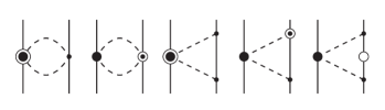
Figure 9: Relativistic corrections of NNLO diagrams. Notation as in Fig. 1. Open circles are relativistic $1/M_{N}$ corrections.

At N³LO, we add the $1/M_{N}$ correction of the NNLO 2PE proportional to $c_{i}$. This correction is proportional to $c_{i}/M_{N}$ (Fig. 9) and appears nominally at fifth order. As discussed, the 2PE bubble diagram proportional to $c_{i}^{2}$ that appears at N³LO is unrealistically attractive, while the $c_{i}/M_{N}$ correction is large and repulsive. Therefore, it makes sense to group these diagrams together to arrive at a more realistic intermediate attraction at N³LO. The contribution is given by Kai01a :

Momentum-space potentials:

$$V_{C}(q) = -\frac{g_{A}^{2}L(q)}{32\pi^{2}M_{N}f_{\pi}^{4}}\bigg{[}(c_{2}-6c_{3})q^{4}+4(6c_{1}+c_{2}-3c_{3})q^{2}m_{\pi}^{2}$$ (147)

$$+6(c_{2}-2c_{3})m_{\pi}^{4}+24(2c_{1}+c_{3})m_{\pi}^{6}w^{-2}\bigg{]}\,,$$

$$W_{C}(q) = -\frac{c_{4}q^{2}L(q)}{192\pi^{2}M_{N}f_{\pi}^{4}}\bigg{[}g_{A}^{2}(8m_{\pi}^{2}+5q^{2})+w^{2}\bigg{]}\,,$$ (148)

$$W_{T}(q) = -\frac{1}{q^{2}}W_{S}(q)=-\frac{c_{4}L(q)}{192\pi^{2}M_{N}f_{\pi}^{4}}\bigg{[}g_{A}^{2}(16m_{\pi}^{2}+7q^{2})-w^{2}\bigg{]}\,,$$ (149)

$$V_{LS}(q) = \frac{c_{2}g_{A}^{2}}{8\pi^{2}M_{N}f_{\pi}^{4}}w^{2}L(q)\,,$$ (150)

$$W_{LS}(q) = -\frac{c_{4}L(q)}{48\pi^{2}M_{N}f_{\pi}^{4}}\left[g_{A}^{2}(8m_{\pi}^{2}+5q^{2})+w^{2}\right]\,.$$ (151)

Spectral functions:

$${\rm Im}V_{C}(i\mu) = \frac{g_{A}^{2}}{64\pi M_{N}f_{\pi}^{4}}\frac{\sqrt{\mu^{2}-4m_{\pi}^{2}}}{\mu}\bigg{[}(c_{2}-6c_{3})\mu^{4}-4(6c_{1}+c_{2}-3c_{3})\mu^{2}m_{\pi}^{2}$$ (152)

$$+6(c_{2}-2c_{3})m_{\pi}^{4}-24(2c_{1}+c_{3})\frac{m_{\pi}^{6}}{\mu^{2}-4m_{\pi}^{2}}\bigg{]}\,,$$

$${\rm Im}W_{C}(i\mu) = -\frac{c_{4}}{384\pi M_{N}f_{\pi}^{4}}\mu\sqrt{\mu^{2}-4m_{\pi}^{2}}\bigg{[}g_{A}^{2}(8m_{\pi}^{2}-5\mu^{2})-\mu^{2}+4m_{\pi}^{2}\bigg{]}\,,$$ (153)

$${\rm Im}W_{T}(i\mu) = \frac{1}{\mu^{2}}{\rm Im}W_{S}(i\mu)=\frac{c_{4}}{384\pi M_{N}f_{\pi}^{4}}\frac{\sqrt{\mu^{2}-4m_{\pi}^{2}}}{\mu}\bigg{[}\mu^{2}-4m_{\pi}^{2}+g_{A}^{2}(16m_{\pi}^{2}-7\mu^{2})\bigg{]}\,,$$ (154)

$${\rm Im}V_{LS}(i\mu) = \frac{c_{2}g_{A}^{2}}{16\pi M_{N}f_{\pi}^{4}}\frac{(\mu^{2}-4m_{\pi}^{2})^{3/2}}{\mu}\,,$$ (155)

$${\rm Im}W_{LS}(i\mu) = \frac{c_{4}}{96\pi M_{N}f_{\pi}^{4}}\frac{\sqrt{\mu^{2}-4m_{\pi}^{2}}}{\mu}\left[g_{A}^{2}(8m_{\pi}^{2}-5\mu^{2})+4m_{\pi}^{2}-\mu^{2}\right]\,.$$ (156)

Position-space potentials:

$$\widetilde{V}_{C}(r) = \frac{3g_{A}^{2}m_{\pi}^{7}}{32\pi^{3}M_{N}f_{\pi}^{4}}\frac{1}{x^{6}}\bigg{[}\bigg{(}20(c_{2}-6c_{3})-4(6c_{1}-c_{2}+9c_{3})x^{2}$$ (157)

$$-2(2c_{1}+c_{3})x^{4}\bigg{)}xK_{0}(2x)+\bigg{(}20(c_{2}-6c_{3})-2(12c_{1}-7c_{2}+48c_{3})x^{2}$$

$$-(16c_{1}-c_{2}+10c_{3})x^{4}\bigg{)}K_{1}(2x)\bigg{]}\,,$$

$$\widetilde{W}_{C}(r) = \frac{c_{4}m_{\pi}^{7}}{32\pi^{3}M_{N}f_{\pi}^{4}}\frac{1}{x^{5}}\bigg{[}\bigg{(}5+25g_{A}^{2}+4g_{A}^{2}x^{2}\bigg{)}xK_{1}(2x)$$ (158)

$$+2\bigg{(}5+25g_{A}^{2}+(1+8g_{A}^{2})x^{2}\bigg{)}K_{2}(2x)\bigg{]}\,,$$

$$\widetilde{W}_{S}(r) = \frac{c_{4}m_{\pi}^{7}}{48\pi^{3}M_{N}f_{\pi}^{4}}\frac{1}{x^{5}}\bigg{[}\bigg{(}5-35g_{A}^{2}-4g_{A}^{2}x^{2}\bigg{)}xK_{1}(2x)$$ (159)

$$+2\bigg{(}5(1-7g_{A}^{2})+(1-10g_{A}^{2})x^{2}\bigg{)}K_{2}(2x)\bigg{]}\,,$$

$$\widetilde{W}_{T}(r) = \frac{c_{4}m_{\pi}^{7}}{192\pi^{3}M_{N}f_{\pi}^{4}}\frac{1}{x^{5}}\bigg{[}2\bigg{(}-8+59g_{A}^{2}+4g_{A}^{2}x^{2}\bigg{)}xK_{1}(2x)$$ (160)

$$-\bigg{(}35(1-7g_{A}^{2})+4(1-13g_{A}^{2})x^{2}\bigg{)}K_{2}(2x)\bigg{]}\,,$$

$$\widetilde{V}_{LS}(r) = \frac{3c_{2}g_{A}^{2}m_{\pi}^{7}}{8\pi^{3}M_{N}f_{\pi}^{4}}\frac{1}{x^{5}}\bigg{[}K_{2}(2x)+2xK_{3}(2x)\bigg{]}\,,$$ (161)

$$\tilde{W}_{LS}(r) = -\frac{c_{4}m_{\pi}^{7}}{16\pi^{3}M_{N}f_{\pi}^{4}}\frac{1}{x^{5}}\bigg{[}(1+6g_{A}^{2})2xK_{1}(2x)+(5+25g_{A}^{2}+4g_{A}^{2}x^{2})K_{2}(2x)\bigg{]}\,.$$ (162)

Appendix B The LECs of the contact terms

Table 7: Values for the contact LECs of the N³LO potentials with cutoff combination $(R_{\pi},R_{\rm ct})=(1.2,0.75)$ fm, $(1.1,0.72)$ fm, and $(1.0,0.70)$ fm. In the column headings, we use the $R_{\pi}$ value to identify the different cases. The notation ($\pm n$) stands for $\times 10^{\pm n}$.

LECs	$R_{\pi}=1.2$ fm	$R_{\pi}=1.1$ fm	$R_{\pi}=1.0$ fm
$C_{c}$ (${\rm fm}^{2}$)	0.28808881 (+1)	0.39582494 (+1)	0.68583069 (+1)
$C_{\tau}$ (${\rm fm}^{2}$)	0.26865444	0.37170364	0.84621879
$C_{\sigma}$ (${\rm fm}^{2}$)	0.37304419 (-1)	0.13087859	0.45593912
$C_{\sigma\tau}$ (${\rm fm}^{2}$)	0.99745306	0.86768636	0.9008921
$C_{1}$ (${\rm fm}^{4}$)	0.20339187 (-1)	-0.69958000 (-1)	-0.19849806
$C_{2}$ (${\rm fm}^{4}$)	-0.26911188 (-1)	-0.73932500 (-2)	0.27128125 (-2)
$C_{3}$ (${\rm fm}^{4}$)	-0.78260937 (-1)	-0.57466500 (-1)	-0.26448938 (-1)
$C_{4}$ (${\rm fm}^{4}$)	-0.35220625 (-2)	-0.13702250 (-1)	-0.89698125 (-2)
$C_{5}$ (${\rm fm}^{4}$)	-0.10596750 (-1)	-0.80355000 (-2)	-0.54697500 (-2)
$C_{6}$ (${\rm fm}^{4}$)	0.31287500 (-2)	0.39985000 (-2)	0.48457500 (-2)
$C_{7}$ (${\rm fm}^{4}$)	-0.84559075	-0.83002375	-0.82673000
$C_{8}$ (${\rm fm}^{4}$)	-0.11612925	-0.10974825	-0.10887000
$D_{1}$ (${\rm fm}^{6}$)	0.27843312 (-1)	0.31251437 (-1)	0.35406750 (-1)
$D_{2}$ (${\rm fm}^{6}$)	-0.11181250 (-3)	0.30660625 (-2)	0.64797500 (-2)
$D_{3}$ (${\rm fm}^{6}$)	0.17309375 (-2)	0.39478125 (-2)	0.28025000 (-2)
$D_{4}$ (${\rm fm}^{6}$)	-0.25564375 (-2)	-0.11373125 (-2)	-0.84200000 (-3)
$D_{5}$ (${\rm fm}^{6}$)	-0.22787500 (-2)	-0.17605000 (-2)	0.13175000 (-3)
$D_{6}$ (${\rm fm}^{6}$)	-0.76425000 (-3)	-0.58650000 (-3)	0.44250000 (-4)
$D_{7}$ (${\rm fm}^{6}$)	0.40027500 (-2)	0.11374250 (-1)	0.70485000 (-2)
$D_{8}$ (${\rm fm}^{6}$)	-0.26426750 (-1)	-0.22689250 (-1)	-0.29755500 (-1)
$D_{9}$ (${\rm fm}^{6}$)	-0.42584000 (-1)	-0.50699750 (-1)	-0.57539750 (-1)
$D_{10}$ (${\rm fm}^{6}$)	-0.14453000 (-1)	-0.16889250 (-1)	-0.19163250 (-1)
$D_{11}$ (${\rm fm}^{6}$)	-0.18565375 (-1)	-0.27816625 (-1)	-0.63730625 (-2)
$D_{12}$ (${\rm fm}^{6}$)	0.16119625 (-1)	0.11181125 (-1)	0.20284813 (-1)
$D_{13}$ (${\rm fm}^{6}$)	0.54308750 (-2)	0.25901250 (-2)	0.77255625 (-2)
$D_{14}$ (${\rm fm}^{6}$)	0.92428750 (-2)	0.76783750 (-2)	0.10042688 (-1)
$C^{\rm CD}_{T_{12}}$ (fm2)	0.30527375 (-2)	0.3081975 (-2)	0.2791292 (-2)
$C^{\rm CD}_{\sigma T_{12}}$ (fm2)	-0.30527375 (-2)	-0.3081975 (-2)	-0.2791292 (-2)
$C^{\rm CA}_{\tau_{z}}$ (fm2)	0.17322500 (-2)	0.20032500 (-2)	0.1817375 (-2)
$C^{\rm CA}_{\sigma\tau_{z}}$ (fm2)	-0.17322500 (-2)	-0.20032500 (-2)	-0.1817375 (-2)

In this Appendix, we show in Table 7 the LECs of the contact terms defined in Sec. II.4 for our N³LO potentials. The shown LECs are the coefficients of the various contact operators displayed in Sec. II.4.

For the fitting of the phase shifts of the different states, it is more convenient to fit to states with well-defined total spin $S$ and total isospin $T$, the (charge-independent) LO coefficients of which we denote by $C_{ST}$. From these $C_{ST}$, one obtains the LECs for the operators used in Eq. (22) via:

$$\left({\begin{array}[]{l}C_{c}\\ C_{\tau}\\ C_{\sigma}\\ C_{\sigma\tau}\end{array}}\right)=\frac{1}{16}\left({\begin{array}[]{rrrr}1&3&3&\;\;9\\ -1&1&-3&3\\ -1&-3&1&3\\ 1&-1&-1&1\end{array}}\right)\left({\begin{array}[]{c}C_{00}\\ C_{01}\\ C_{10}\\ C_{11}\end{array}}\right)$$ (163)

Similar relations apply to the central force LECs of higher order, like the $C_{1}$ to $C_{4}$ of Eq. (27) and the $D_{1}$ to $D_{4}$ of Eq. (35); as well to the coefficients of the four ${\vec{L}}^{2}$ terms, $D_{11}$ to $D_{14}$ [Eq. (35)].

Vice versa, the spin-isospin coefficients can be obtained from the operator LECs via:

$$\left({\begin{array}[]{c}C_{00}\\ C_{01}\\ C_{10}\\ C_{11}\end{array}}\right)=\left({\begin{array}[]{rrrr}1&-3&-3&9\\ 1&1&-3&-3\\ 1&-3&1&-3\\ 1&1&1&1\end{array}}\right)\left({\begin{array}[]{l}C_{c}\\ C_{\tau}\\ C_{\sigma}\\ C_{\sigma\tau}\end{array}}\right)$$ (164)

Tensor, spin-orbit, and quadratic spin-orbit terms exist only in $S=1$ states, such that one needs to distinguish only between a $T=0$ and $T=1$ channel. For example, in the case of the NLO tensor force, the relations are:

$$C_{5}\,\equiv\,C_{S_{12}} = \frac{1}{4}\left(C_{10}^{(S_{12})}+3C_{11}^{(S_{12})}\right)\,,$$

$$C_{6}\,\equiv\,C_{S_{12}\tau} = \frac{1}{4}\left(-C_{10}^{(S_{12})}+C_{11}^{(S_{12})}\right)\,,$$ (165)

and vice versa

$$C_{10}^{(S_{12})} = C_{S_{12}}-3C_{S_{12}\tau}=C_{5}-3C_{6}\,,$$

$$C_{11}^{(S_{12})} = C_{S_{12}}+C_{S_{12}\tau}=C_{5}+C_{6}\,,$$ (166)

and similarly for the other cases that appear only at $S=1$.

To reproduce the three charge dependent ${}^{1}S_{0}$ scattering lenghts, the LO contact LEC with $(S,T)=(0,1)$ is fit in a charge-dependent way. Thus, this LEC comes in three versions: $C_{01}^{pp}$, $C_{01}^{np}$, and $C_{01}^{nn}$. In tune with Eqs. (22) and (23), the charge-dependent LEC can be represented by

$$C_{01}^{NN} = C_{01}+C_{01}^{\rm CD}T_{12}+C_{01}^{\rm CA}(\tau_{1z}+\tau_{2z})$$ (167)

with $T_{12}$ defined in Eq. (21). $C_{01}$ denotes the charge-independent value, which is fixed by

$$C_{01} = \frac{1}{3}\left(C_{01}^{pp}+C_{01}^{np}+C_{01}^{nn}\right)\,,$$ (168)

while the charge-dependent ones are

$$C_{01}^{\rm CD} = \frac{1}{6}\left[\frac{1}{2}\left(C_{01}^{pp}+C_{01}^{nn}\right)-C_{01}^{np}\right]\,\,\mbox{\rm and}$$ (169)

$$C_{01}^{\rm CA} = \frac{1}{4}\left(C_{01}^{pp}-C_{01}^{nn}\right)\,.$$ (170)

By analogy to Eqs. (165), the operator LECs used in Eq. (23) can be obtained from the channel LECs through:

$$C_{T_{12}}^{\rm CD} = \frac{1}{4}\left(C_{01}^{\rm CD}+3C_{11}^{\rm CD}\right)\,,$$

$$C_{\sigma T_{12}}^{\rm CD} = \frac{1}{4}\left(-C_{01}^{\rm CD}+C_{11}^{\rm CD}\right)\,.$$ (171)

We do not assume any charge dependence for the contacts in $S=1,T=1$ states (triplet $P$-waves); therefore, we have $C_{11}^{\rm CD}=0$. Thus,

$$C_{T_{12}}^{\rm CD} = \frac{1}{4}\left(C_{01}^{\rm CD}\right)\,,$$

$$C_{\sigma T_{12}}^{\rm CD} = \frac{1}{4}\left(-C_{01}^{\rm CD}\right)\,.$$ (172)

Similar relations apply to charge asymmetry,

$$C_{\tau_{z}}^{\rm CA} = \frac{1}{4}\left(C_{01}^{\rm CA}+3C_{11}^{\rm CA}\right)\,,$$

$$C_{\sigma\tau_{z}}^{\rm CA} = \frac{1}{4}\left(-C_{01}^{\rm CA}+C_{11}^{\rm CA}\right)\,.$$ (173)

Also here, we do not assume any charge asymmetry for the contacts in $S=1,T=1$ states; thus, $C_{11}^{\rm CA}=0$; hence

$$C_{\tau_{z}}^{\rm CA} = \frac{1}{4}\left(C_{01}^{\rm CA}\right)\,,$$

$$C_{\sigma\tau_{z}}^{\rm CA} = \frac{1}{4}\left(-C_{01}^{\rm CA}\right)\,.$$ (174)

A final aspect to discuss is the question to what extend the LECs are natural. LECs may be perceived as natural if they are of the following magnitudes:

$$|C_{c,\tau,\sigma,\sigma\tau}| \sim \frac{1}{f_{\pi}^{2}}\approx 5\,\,\mbox{\rm fm}^{2}\,,$$ (175)

$$|C_{i}| \sim \frac{1}{f_{\pi}^{2}\,\Lambda_{b}^{2}}\approx 0.4\,\,\mbox{\rm fm}^{4}\,,$$ (176)

$$|D_{i}| \sim \frac{1}{f_{\pi}^{2}\,\Lambda_{b}^{4}}\approx 0.03\,\,\mbox{\rm fm}^{6}\,,$$ (177)

with $\Lambda_{b}\approx m_{\rho}\approx$ 0.7 GeV the breakdown scale Fur15 .

Comparing these estimates with the values shown in Table 7 reveals that our contact LECs are, in general, natural. At zeroth order, $C_{c}$ is certainly of the right order, and the $C_{\tau,\sigma,\sigma\tau}$ are around one, which is close enough to the estimate. At second order, $C_{1}$ and the $LS$ force parameters, $C_{7}$ and $C_{8}$ are of the right size, while the other LECs are on the smaller side. Finally at fourth order, $D_{1}$, the $LS$ parameter $D_{8}$, the $(LS)^{2}$ parameters $D_{9}$ and $D_{10}$, and the $L^{2}$ LECs $D_{12}$ and $D_{14}$ come out natural, whereas the other $D_{i}$ emerge in small format.

Appendix C Potential plots

In this appendix, we show figures for the various components of the chiral $NN$ potentials and contrast them with some well known traditional phenomenology.

In Fig. 10, we compare the four central-potential components (notation as in Eq. (63), but without the tilde) as predicted by the chiral potentials at NNLO and N³LO (green dashed and red solid lines, respectively) with two phenomenological potentials, namely, the AV18 potential WSS95 and a one-boson-exchange potential (OBEP) note1 (black dotted and blue dash-dotted lines, respectively). The chiral potentials apply the cutoff combination $(R_{\pi},R_{\rm ct})=(1.0,0.70)$ fm. While at short range ($r<1$ fm) there are large differences between the models, there is qualitative agreement between most models in the (more important) intermediate range ($1<r<2$ fm) as revealed in the right side of Fig. 10. In particular, there is good agreement between the N³LO potential and AV18, providing support from chiral EFT for the AV18 potential.

From the left $V_{C}$ panel of Fig. 10, it may appear that OBEP (blue dash-dotted curve) does not create a hard core (repulsive short range force). This is misleading, because a hard core is needed for the $S$-wave states. For the ${}^{1}S_{0}$ state, the $V_{S}$ and the $W_{S}$ potentials are multiplied by a factor of $(-3)$, which creates strong short-range repulsion (cf. Fig. 13 below). For ${}^{3}S_{1}$, $W_{C}$ and $W_{S}$ are multiplied by $(-3)$ producing the hard core.

Tensor potentials as shown in Fig. 11. It is clearly seen that the chiral tensor potentials are much weaker than, particularly, the AV18. Note that, in the case of OBEP (blue dash-dotted lines), the negative short-range potential of $V_{T}$ is essentially due to the $\omega$ meson and a similar curve in $W_{T}$ is due to the $\rho$ meson. Both these heavy vector mesons have no place in chiral EFT, which is why the chiral EFT predictions are essentially flat in the short-range region (unless there were large tensor contact contributions, which our chiral potentials do not carry). The $W_{T}$ tensor force in the intermediate- and long-range region is generated from 1PE for all models, which is why there is agreement between all models above $r>1$ fm.

The eight potential components that depend on the orbital angular momentum operator $\vec{L}$ are displayed in Fig. 12. For $V_{LS}$ and $W_{LS}$ there is qualitative agreement between all models. Triplet $P$ waves cannot be described quantitatively without a proper strong spin-orbit force, which is presumably the reason for this agreement. Note that the chiral potential at NNLO and OBEP do not have $(\vec{L}\cdot\vec{S})^{2}$ and ${\vec{L}}^{2}$ components. For the $(\vec{L}\cdot\vec{S})^{2}$ potentials, there is rough agreement between N³LO and AV18 for $r>0.5$ fm. On the other hand, the four ${\vec{L}}^{2}$ potentials appear erratic. Obviously, these components of the nuclear force are not well pinned down. They are also small, which may be why they are not so relevant and hard to pin down.

Some important partial-wave potentials are shown in Fig. 13. In the ${}^{1}S_{0}$ state, all models exhibit a strong short-range repulsion, the size of which, however, differs dramatically. Nevertheless, there is agreement between the models in the (more relevant) range above 0.5 fm as demonstrated in the second ${}^{1}S_{0}$ frame of the figure. The differences in size of the tensor forces of different models is best demonstrated by way of the ${}^{3}S_{1}$-${}^{3}D_{1}$ transition potential, which we show in the third panel of Fig. 13. The AV18 potential has the strongest tensor force, OBEP is second, and NNLO and N³LO have the weakest. As discussed, for $r>1$ fm, 1PE is the dominant tensor force in all models, which is why all models agree in that region.

Finally, we also wish to provide some idea for the cutoff dependence of the chiral potentials. For that purpose we show, in Fig. 14, the ${}^{1}S_{0}$ and ${}^{3}S_{1}$-${}^{3}D_{1}$ potentials at N³LO for the cutoff combinations $(R_{\pi},R_{\rm ct})=(1.0,0.70)$ fm, $(1.1,0.72)$ fm, and $(1.2,0.75)$ fm (solid, dashed, and dotted curves, respectively). The short-range parts of the ${}^{1}S_{0}$ potentials exemplify the effect of the short-range cutoff on the central forces, Eqs. (24), (29), and (36), (ruled by $R_{\rm ct}$), while the ${}^{3}S_{1}$-${}^{3}D_{1}$ potentials demonstrate the impact of the long-range regulator function, Eq. (52), (governed by $R_{\pi}$).

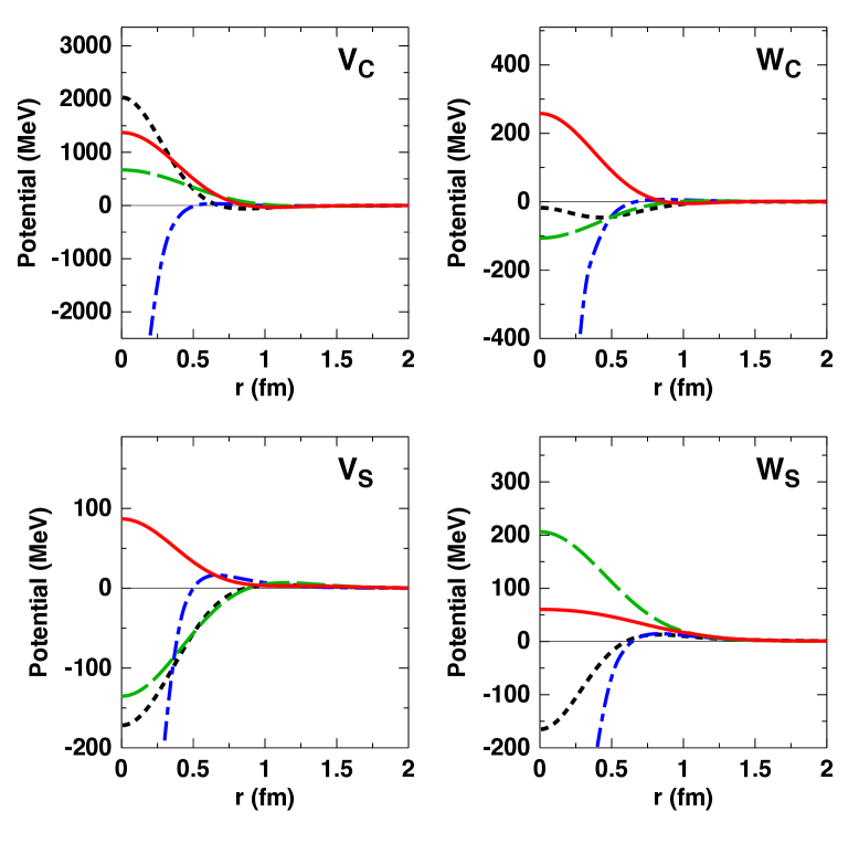
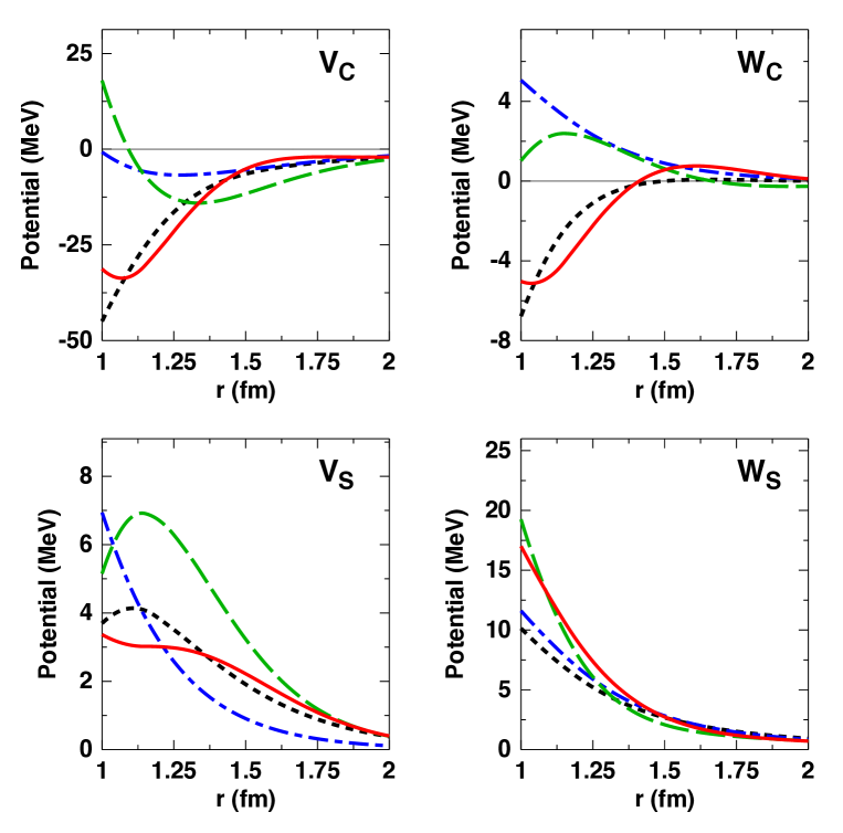
Figure 10: Left side: The four central potentials in the range 0 to 2 fm. Right side: The same in the range 1 to 2 fm. To mark the various potential components, the notation of Eq. (63) is used (with the tilde omitted). Predictions are shown for the AV18 potential WSS95 (black dotted line), an OBEP note1 (blue dash-dotted line), the chiral NNLO potential of this work (green dashed line), and the chiral N³LO potential of this work (red solid line). For the chiral potentials, the cutoff combination $(R_{\pi},R_{\rm ct})=(1.0,0.70)$ fm is used.

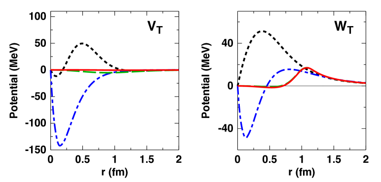
Figure 11: The tensor potentials. Notation as in Fig. 10.

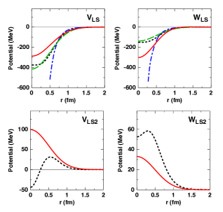
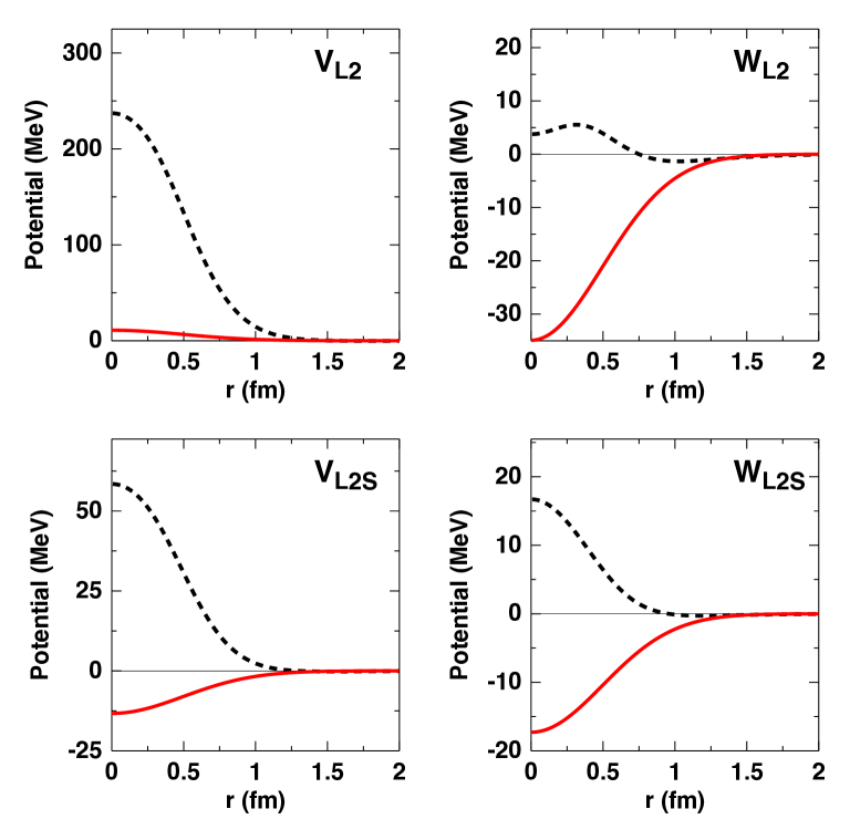
Figure 12: The eight $\vec{L}$-dependent potentials. Notation as in Fig. 10. Moreover, $LS2$ stands for $(\vec{L}\cdot\vec{S})^{2}$, $L2$ for ${\vec{L}}^{2}$, and $L2S$ for ${\vec{L}}^{2}\vec{\sigma}_{1}\cdot\vec{\sigma}_{2}$. Note that the OBEP and the chiral potential at NNLO do not include $(\vec{L}\cdot\vec{S})^{2}$ and ${\vec{L}}^{2}$ components.

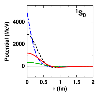
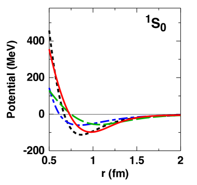
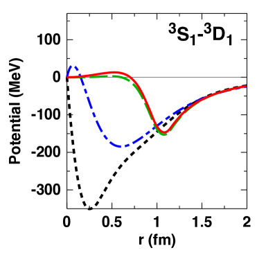
Figure 13: The ${}^{1}S_{0}$ potential in the range 0 to 2 fm and 0.5 to 2 fm, as well as the ${}^{3}S_{1}$-${}^{3}D_{1}$ potential in the range 0 to 2 fm. Notation as in Fig. 10.

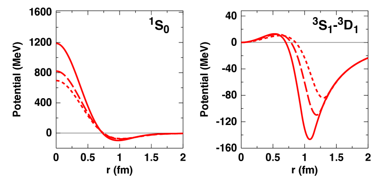
Figure 14: Cutoff dependence of the ${}^{1}S_{0}$ and ${}^{3}S_{1}$-${}^{3}D_{1}$ chiral potentials at N³LO. The cutoff combinations $(R_{\pi},R_{\rm ct})=(1.0,0.70)$ fm, $(1.1,0.72)$ fm, and $(1.2,0.75)$ fm are shown by the solid, dashed, and dotted curves.

References

- (1) R. Machleidt and D. R. Entem, Phys. Rep. 503, 1 (2011).
- (2) E. Epelbaum, H.-W. Hammer, and U.-G. Meißner, Rev. Mod. Phys. 81, 1773 (2009).
- (3) H.-W. Hammer, S. Kőnig, and U. van Kolck, Rev. Mod. Phys. 92, 025004 (2020).
- (4) K. Hebeler, Phys. Rept. 890, 1 (2021).
- (5) J. Carlson, S. Gandolfi, F. Pederiva, S. C. Pieper, R. Schiavilla, K. E. Schmidt, and R. B. Wiringa, Rev. Mod. Phys. 87, 1067 (2015).
- (6) J. E. Lynn, I. Tews, S. Gandolfi, and A. Lovato, Ann. Rev. Nucl. Part. Sci. 69, 279-305 (2019).
- (7) M. Piarulli and I. Tews, Front. in Phys. 7, 245 (2020).
- (8) A. Gezerlis, I. Tews, E. Epelbaum, M. Freunek, S. Gandolfi, K. Hebeler, A. Nogga, and A. Schwenk, Phys. Rev. C 90, no.5, 054323 (2014).
- (9) M. Piarulli, L. Girlanda, R. Schiavilla, R. Navarro Pérez, J. E. Amaro, and E. Ruiz Arriola, Phys. Rev. C 91, no.2, 024003 (2015).
- (10) M. Piarulli, L. Girlanda, R. Schiavilla, A. Kievsky, A. Lovato, L. E. Marcucci, S. C. Pieper, M. Viviani, and R. B. Wiringa, Phys. Rev. C 94, no.5, 054007 (2016).
- (11) C. Ordóñez, L. Ray, and U. van Kolck, Phys. Rev. Lett. 72, 1982 (1994).
- (12) C. Ordóñez, L. Ray, and U. van Kolck, Phys. Rev. C 53, 2086 (1996).
- (13) V. Bernard, N. Kaiser and U. G. Meissner, Nucl. Phys. A 615, 483 (1997).
- (14) N. Kaiser, S. Gerstendőrfer, and W. Weise, Nucl. Phys. A637, 395 (1998).
- (15) H. Krebs, E. Epelbaum, and U. G. Meissner, Eur. Phys. J. A 32, 127 (2007).
- (16) H. Krebs, A. M. Gasparyan, and E. Epelbaum, Phys. Rev. C 98, 014003 (2018).
- (17) W. G. Jiang, A. Ekström, C. Forssén, G. Hagen, G. R. Jansen, and T. Papenbrock, Phys. Rev. C 102, 054301 (2020).
- (18) Y. Nosyk, D. R. Entem, and R. Machleidt, Phys. Rev. C 104, 054001 (2021).
- (19) R. J. Furnstahl, N. Klco, D. R. Phillips, and S. Wesolowski, Phys. Rev. C 92, 024005 (2015).
- (20) S. Weinberg, Phys. Lett B251, 288 (1990); Nucl. Phys. B363, 3 (1991).
- (21) N. Kaiser, Phys. Rev. C 61, 014003 (2000).
- (22) N. Kaiser, Phys. Rev. C 62, 024001 (2000).
- (23) D. R. Entem and R. Machleidt, Phys. Rev. C 66, 014002 (2002).
- (24) D. R. Entem and R. Machleidt, Phys. Rev. C 68, 041001 (2003).
- (25) F. Sammarruca, L. Coraggio, J. W. Holt, N. Itaco, R. Machleidt, and L. E. Marcucci, Phys. Rev. C 91, 054311 (2015).
- (26) E. Epelbaum, H. Krebs, and Ulf-G. Meißner, Eur. Phys. J. A 51, 53 (2015).
- (27) D. R. Entem, R. Machleidt, and Y. Nosyk, Phys. Rev. C 96, 024004 (2017).
- (28) M. Hoferichter, J. Ruiz de Elvira, B. Kubis, and U.-G. Meißner, Phys. Rev. Lett. 115, 192301 (2015); Phys. Rep. 625, 1 (2016).
- (29) P.A. Zyla et al. (Particle Data Group), Prog. Theor. Exp. Phys. 2020, 083C01 (2020).
- (30) S. Okubo and R. E. Marshak, Ann. Phys. (N.Y.) 4, 166 (1958).
- (31) M. Fierz, Z. Physik 104, 553 (1937).
- (32) L. Huth, I. Tews, J. E. Lynn, and A. Schwenk, Phys. Rev. C 96, no.5, 054003 (2017).
- (33) R. B. Wiringa, V. G. J. Stoks, and R. Schiavilla, Phys. Rev. C 51, 38-51 (1995).
- (34) G. J. M. Austin and J. J. de Swart, Phys. Rev. Lett. 50, 2039 (1983).
- (35) J. R. Bergervoet, P. C. van Campen, W. A. van der Sanden, and J. J. de Swart, Phys. Rev. C 38, 15 (1988).
- (36) U. van Kolck, M. C. M. Rentmeester, J. L. Friar, T. Goldman, and J. J. de Swart, Phys. Rev. Lett. 80, 4386 (1998).
- (37) R. Blankenbecler and R. Sugar, Phys. Rev. 142, 1051 (1966).
- (38) M. M. Nagels, Baryon-Baryon Scattering in a One-Boson-Exchange Potential Model, Ph.D. thesis, University of Nijmegen (1975).
- (39) H. Shimoyama, Chiral Symmetry and the Nucleon-Nucleon Interaction: Developing a Chiral NN Potential in Configuration Space, Ph.D. thesis, University of Idaho (2005).
- (40) P. Herd, Local Nucleon-Nucleon Potentials Based upon Chiral Effective Field Theory, Master of Science Thesis, University of Idaho (2015).
- (41) Prog. Theor. Phys. (Kyoto), Suppl. 3 (1956).
- (42) T. E. O. Ericson and M. Rosa-Clot, Nucl. Phys. A 405, 497 (1983).
- (43) R. Machleidt, Adv. Nucl. Phys. 19, 189 (1989).
- (44) R. Machleidt, K. Holinde, and Ch. Elster, Phys. Rep. 149, 1 (1987).
- (45) R. Vinh Mau, “The Paris Nucleon-Nucleon Interaction”, in: Mesons in Nuclei, Vol. I, eds. M. Rho and D. H. Wilkinson (North-Holland, Amsterdam, 1979) pp. 151-196.
- (46) V. G. J. Stoks, R. A. M. Klomp, M. C. M. Rentmeester, and J. J. de Swart, Phys. Rev. C 48, 792 (1993).
- (47) D. E. González Trotter et al., Phys. Rev. C 73, 034001 (2006).
- (48) Q. Chen et al., Phys. Rev. C 77, 054002 (2008).
- (49) R. A. Arndt, W. J. Briscoe, I. I. Strakovsky, and R. L. Workman, Phys. Rev. C 76, 025209 (2007).
- (50) W. A. van der Sanden, A. H. Emmen, and J. J. de Swart, Report No. THEF-NYM-83.11, Nijmegen (1983), unpublished; quoted in Ref. Ber88 .
- (51) R. C. Malone et al., Measurement of the Neutron-Neutron Quasifree Scattering Cross Section in Neutron-Deuteron Breakup at 10.0 and 15.6 MeV, arXiv:2203.02619 [nucl-ex].
- (52) R. Machleidt, Phys. Rev. C 63, 024001 (2001).
- (53) V. G. J. Stoks and J. J. de Swart, Phys. Rev. C 42, 1235 (1990).
- (54) V. G. J. Stoks (private communication).
- (55) V. G. J. Stoks, R. A. M. Klomp, C. P. F. Terheggen, and J. J. de Swart, Phys. Rev. C 49, 2950-2962 (1994).
- (56) P. Reinert, H. Krebs, and E. Epelbaum, Eur. Phys. J. A 54, no.5, 86 (2018).
- (57) R. Navarro Pérez, J. E. Amaro, and E. Ruiz Arriola, Phys. Rev. C 88, no.6, 064002 (2013).
- (58) S. Klarsfeld, J. Martorell and D. W. L. Sprung, J. Phys. G 10, 165-179 (1984).
- (59) L. Mathelitsch and B. J. Verwest, Phys. Rev. C 29, 739-746 (1984).
- (60) J. J. de Swart, C. P. F. Terheggen and V. G. J. Stoks, [arXiv:nucl-th/9509032 [nucl-th]].
- (61) R. J. Furnstahl, D. R. Phillips, and S. Wesolowski, J. Phys. G 42, 034028 (2015).
- (62) R. Navarro Perez, J. E. Amaro, and E. Ruiz Arriola, Phys. Rev. C 89, 064006 (2014).
- (63) R. Navarro Perez, E. Garrido, J. E. Amaro, and E. Ruiz Arriola, Phys. Rev. C 90, 047001 (2014).
- (64) R. Navarro Perez, J. E. Amaro, E. Ruiz Arriola, P. Maris, and J. P. Vary, Phys. Rev. C 92, 064003 (2015).
- (65) E. Marji et al., Phys. Rev. C 88, 054002 (2013).
- (66) E. Epelbaum, A. Nogga, W. Gloeckle, H. Kamada, U. G. Meissner, and H. Witala, Phys. Rev. C 66, 064001 (2002).
- (67) A. Nogga, P. Navratil, B. R. Barrett, and J. P. Vary, Phys. Rev. C 73 (2006) 064002.
- (68) K. Hebeler, S. K. Bogner, R. J. Furnstahl, A. Nogga, and A. Schwenk, Phys. Rev. C 83, 031301(R) (2011).
- (69) A. Gårdestig and D. R. Philips, Phys. Rev. Lett. 96 (2006) 232301.
- (70) D. Gazit, S. Quaglioni, and P. Navrátil, Phys. Rev. Lett. 103 (2009) 102502.
- (71) L. E. Marcucci, A. Kievsky, S. Rosati, R. Schiavilla, and M. Viviani, Phys. Rev. Lett. 108, 052502 (2012).
- (72) P. Navratil, V. G. Gueorguiev, J. P. Vary, W. E. Ormand, and A. Nogga, Phys. Rev. Lett. 99 (2007) 042501.
- (73) T. Krűger, I. Tews, K. Hebeler, and A. Schwenk, Phys. Rev. C 88, 025802 (2013).
- (74) C. Drischler, K. Hebeler, and A. Schwenk, Phys. Rev. C 93, 054314 (2016).
- (75) C. Drischler, A. Carbone, K. Hebeler, and A. Schwenk, Phys. Rev. C 94, 054307 (2016).
- (76) A user-friendly FORTRAN code for all potentials presented in this paper can be obtained from one of the authors (R.M.) upon request.
- (77) N. Kaiser, R. Brockmann, and W. Weise, Nucl. Phys. A625, 758 (1997).
- (78) N. Kaiser, Phys. Rev. C 64, 057001 (2001).
- (79) D. R. Entem, N. Kaiser, R. Machleidt, and Y. Nosyk, Phys. Rev. C 91, 014002 (2015).
- (80) The OBEPR presented in Appendix F of of Ref. MHE87 is used.