Globally Optimal Event-Based Divergence Estimation for Ventral Landing

Abstract

Event sensing is a major component in bio-inspired flight guidance and control systems. We explore the usage of event cameras for predicting time-to-contact (TTC) with the surface during ventral landing. This is achieved by estimating divergence (inverse TTC), which is the rate of radial optic flow, from the event stream generated during landing. Our core contributions are a novel contrast maximisation formulation for event-based divergence estimation, and a branch-and-bound algorithm to exactly maximise contrast and find the optimal divergence value. GPU acceleration is conducted to speed up the global algorithm. Another contribution is a new dataset containing real event streams from ventral landing that was employed to test and benchmark our method. Owing to global optimisation, our algorithm is much more capable at recovering the true divergence, compared to other heuristic divergence estimators or event-based optic flow methods. With GPU acceleration, our method also achieves competitive runtimes.

1 Introduction

Flying insects employ seemingly simple sensing and processing mechanisms for flight guidance and control. Notable examples include the usage of observed optic flow (OF) by honeybees for flight control and odometry [48], and observed OF asymmetries for guiding free flight behaviours in fruit flies [54]. Taking inspiration from insects to build more capable flying machines [17, 49, 50], a branch of biomimetic engineering, is an active research topic.

The advent of event sensors [10, 28, 42] has helped push the boundaries of biomimetic engineering. Akin to biological eyes, a pixel in an event sensor asynchronously triggers an event when the intensity change at that pixel exceeds a threshold. An (ideal) event sensor outputs a stream of events if it observes continuous changes, e.g., due to motion, else it generates nothing. The asynchronous pixels also enable higher dynamic range and lower power consumption. These qualities make event sensors attractive as flight guidance sensors for aircraft [13, 15, 32, 41, 45, 57] and spacecraft [35, 47, 55, 56].

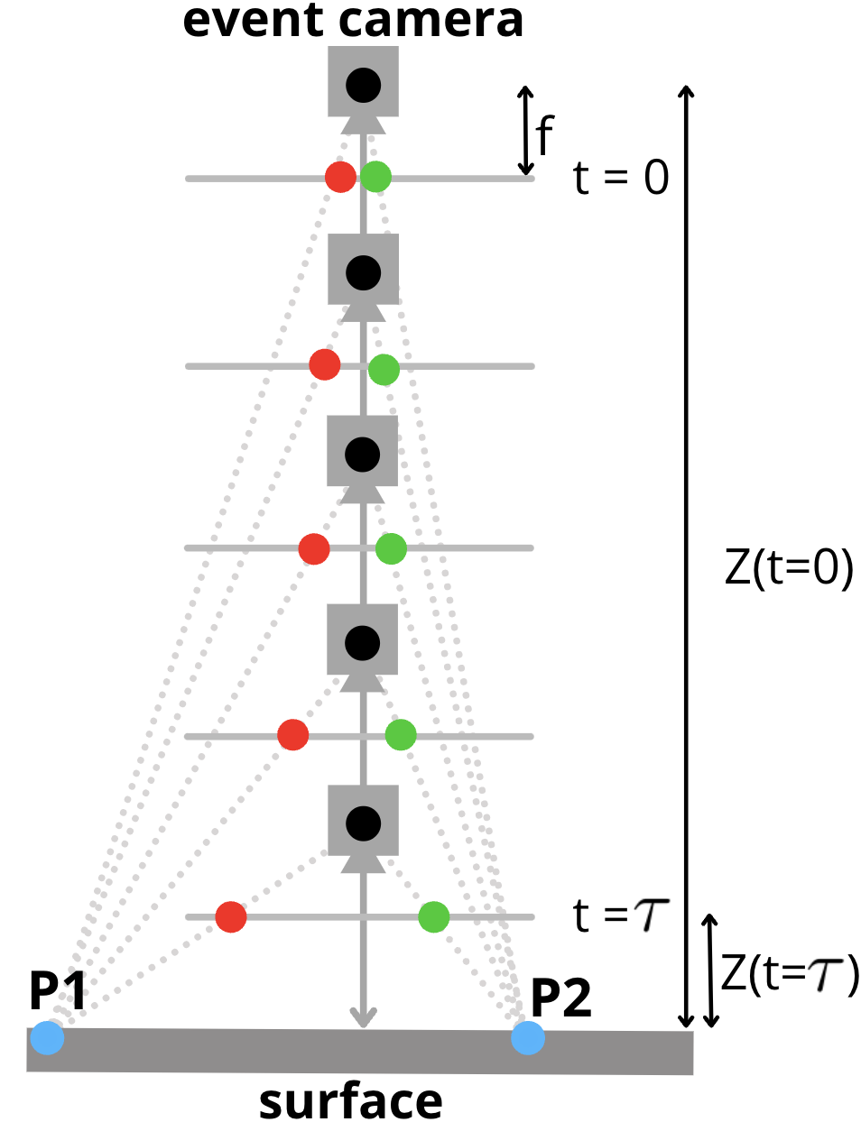
(a)

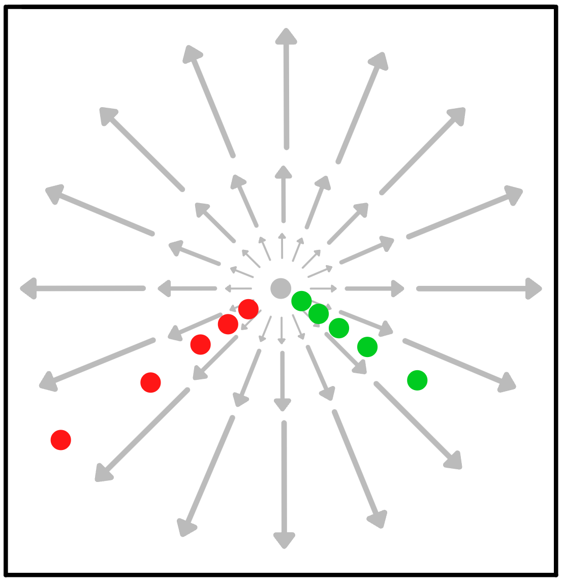
(b)

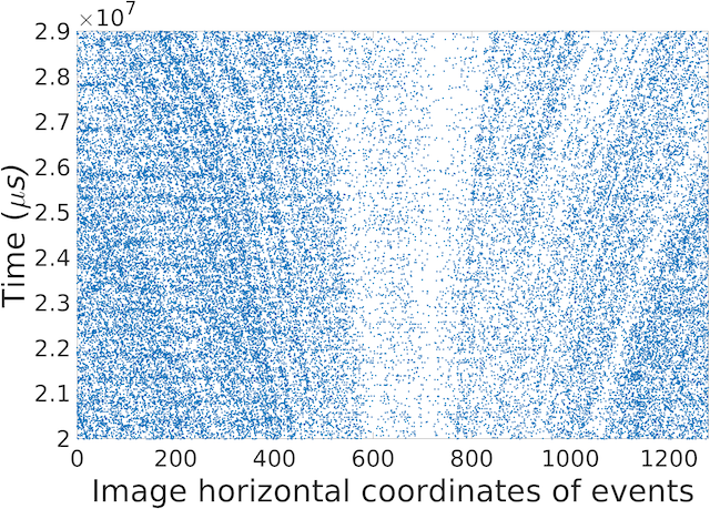
(c)

Figure 1: (a) An event camera with focal length $f$ undergoing ventral descent to a surface over time $0$ to $\tau$ seconds. (b) Two example event trajectories triggered by observation of scene points $P1$ and $P2$ on the surface. The event trajectories are asynchronous observations of the radial optic flows, which emanate from the focus of expansion (FOE). (c) Actual event data produced under ventral descent (only the image horizontal coordinates and event time stamps are shown here).

In previous works, divergence is typically recovered from the OF vectors resulting from event-based OF estimation [41, 47, 55, 56]. However, OF estimation is challenged by noise in the event data (see Fig. 2(b)), which leads to inaccurate divergence estimates (as we will show in Sec. 6). Fundamentally, OF estimation, which usually includes detecting and tracking features, is more complex than estimating divergence (a scalar quantity).

1.0.1 Our contributions

We present a contrast maximisation [18, 53] formulation for event-based divergence estimation. We examined the geometry of ventral landing and derived event-based radial flow, then built a mathematically justified optimisation problem that aims to maximise the contrast of the flow-compensated image; see Fig. 2. To solve the optimisation, we developed an exact algorithm based on branch-and-bound (BnB) [24], which is accelerated using GPU.

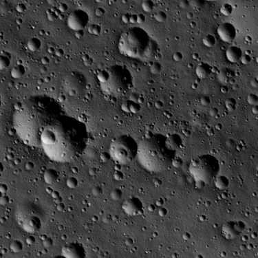
(a)

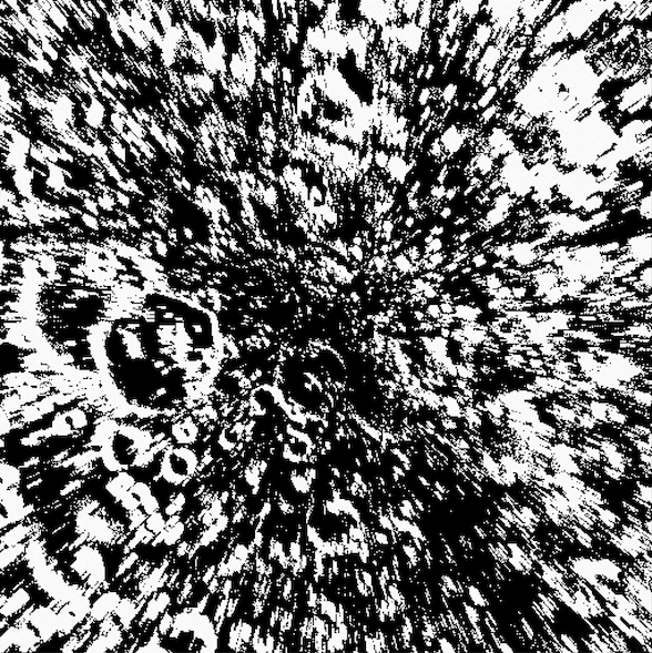
(b)

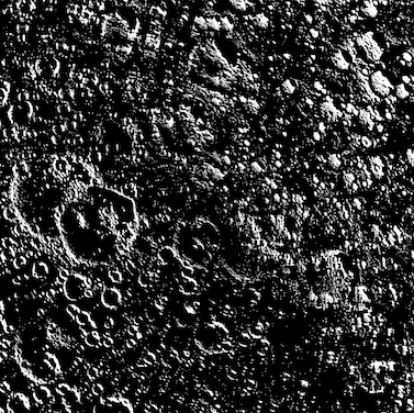
(c)

Figure 2: (a) Intensity image of landing surface. (b) Event image (without motion compensation) for a batch of events generated while observing the surface during vertical landing (image contrast is 0.15). (c) Motion compensated event image produced by our divergence estimation method (image contrast is 0.44).

Since our aim is divergence estimation, our mathematical formulation differs significantly from the exact methods of [29, 40], who focused on different problems. More crucially, our work establishes the practicality of exact contrast maximisation through GPU acceleration, albeit on a lower dimensional problem.

To test our method, we collected real event data from ventral landing scenarios (Sec. 5), where ground truth values were produced through controlled recording using a robot arm and depth sensing. Results in Sec. 6 show that our method is much more accurate than previous divergence estimators [41, 47] that conduct heuristic OF recovery (plane fitting, centroid tracking). Our method also exhibited superior accuracy over state-of-the-art event-based OF methods [20, 51, 53] that we employed for divergence estimation. The usage of GPU acceleration enabled our global method to achieve competitive runtimes.

2 Related work

2.0.1 Event-based optic flow

Event-based OF is a rapidly growing area in computer vision. Some event-based OF approaches [7, 37] are based on the traditional brightness constancy assumption. Other methods [9, 18] expand on the Lucas and Kanade algorithm [31], which assumes constant, localised flow. Alternative approaches include pure event-based time oriented OF estimations [8], computing distance transforms as input to intensity-based OF algorithms [6], and adaptive block matching where OF is computed a points where brightness changes [30]. An extension of event-based OF is event-based motion segmentation [52, 53, 59], where motion models are fitted to clusters of events that have the same OF.

Learning methods for event-based OF train deep neural networks (DNNs) to output event image OF estimations from input representations of event point clouds. Some of these methods require intensity frames in addition to the event data [14, 60, 61], whereas others require event data only [19, 20, 58]. Closely relevant are image and video reconstruction from event methods [38, 43, 44, 46], which employ frame-based and event-based OF techniques. Note that not all event sensors provide intensity frames and event streams.

2.0.2 Event-based divergence estimation

Using event cameras for flight guidance (e.g., attitude estimation, aerial manoeuvres) is an active research area [11, 12, 21, 35]. The focus of our work is event-based divergence estimation, which is useful for guiding the ventral descent of aircraft [41] and spacecraft [47].

Pijnacker-Hordijk et al. [41] employed and extended the plane fitting method of [8] for event-based divergence estimation. The algorithm was also embedded in a closed-loop vertical landing system of an MAV. In the context of planetary landing, Sikorski et al. [47] presented a local feature matching and tracking method, which was also embedded in a closed-loop guidance system. However, their system was evaluated only on simulated event data [47].

Since our focus is on the estimation of divergence, we will distinguish against the state-of-the-art methods [41, 47] only in that aspect, i.e., independently of a close-loop landing system. As we will show in Sec. 6, our globally optimal contrast maximisation approach provides much more accurate estimates than [41, 47].

2.0.3 Spiking neural networks

Further pushing the boundaries of biomimetic engineering is the usage of spiking neural networks (SNN) [36] for event-based OF estimation [22, 23, 27, 39]. Due to the limited availability of SNN hardware [26], we consider only off-the-shelf computing devices (CPUs and GPUs) in our work, but we note that SNNs are attractive future research.

3 Geometry of ventral landing

We first examine the geometry of ventral descent and derive continuous radial OF and divergence, before developing the novel event-based radial flow.

3.1 Continuous-time optic flow

Let $\textbf{P}(t)=\left[\begin{matrix}X(t),&Y(t),&Z(t)\end{matrix}\right]^{T}$ be a 3D scene point that is moving with velocity $\mathbf{V}(t)=\left[\begin{matrix}V_{X}(t),&V_{Y}(t),&V_{Z}(t)\end{matrix}\right]^{T}$. Assuming a calibrated camera, projecting $\mathbf{P}(t)$ onto the image plane yields a moving image point

$$\textbf{p}(t)=\begin{bmatrix}x(t),&y(t)\end{bmatrix}^{T}:=\left[\begin{matrix}fX(t)/Z(t),&fY(t)/Z(t)\end{matrix}\right]^{T},$$ (1)

where $f$ is the focal length of the event camera. Differentiating $\mathbf{p}(t)$ yields the continuous-time OF of the point, i.e.,

$$\textbf{v}(t)=\begin{bmatrix}\dfrac{fV_{X}(t)-V_{Z}(t)x(t)}{Z(t)},&\dfrac{fV_{Y}(t)-V_{Z}(t)y(t)}{Z(t)}\end{bmatrix}.$$ (2)

Note that the derivations above are standard; see, e.g., [16, Chapter 10].

3.2 Continuous-time radial flow and divergence

Following [41, 47], we consider the ventral landing scenario depicted in Fig. 1(a). The setting carries the following assumptions:

• All scene points lie on a fronto-parallel flat surface; and

• The camera has no horizontal motion, i.e., $V_{X}(t)=V_{Y}(t)=0$, which implies that $\textbf{P}(t)=\left[\begin{matrix}X,&Y,&Z(t)\end{matrix}\right]^{T}$, i.e., the first two elements of $\mathbf{P}(t)$ are constants.

Sec. 6 will test our ideas using real data which unavoidably deviated from the assumptions. Under ventral landing, (2) is simplified to

$$\textbf{v}(t)=-\left[V_{Z}(t)/Z(t)\right]\mathbf{p}(t).$$ (3)

Since the camera is approaching the surface, $V_{Z}(t)\leq 0$, hence $\mathbf{v}(t)$ points away from $\mathbf{0}$ (the FOE) towards the direction of $\mathbf{p}(t)$; see Fig. 1(b).

The continuous-time divergence is the quantity

$$D(t)=V_{Z}(t)/Z(t),$$ (4)

which is the rate of expansion of the radial OF. The divergence is independent of the scene point $\mathbf{P}(t)$, and the inverse of $D(t)$, i.e., distance to surface over rate of approach to the surface, is the instantaneous TTC.

3.3 Event-based radial flow

Let $\mathcal{S}$ be an event stream generated by an event camera during ventral descent. Following previous works, e.g. [18, 37, 52], we separate $\mathcal{S}$ into small finite-time sequential batches. Let $\mathcal{E}=\{\mathbf{e}_{i}\}^{N}_{i=1}\subset\mathcal{S}$ be a batch with $N$ events, where each $\mathbf{e}_{i}=(x_{i},y_{i},t_{i},p_{i})$ contains image coordinates $(x_{i},y_{i})$, time stamp $t_{i}$ and polarity $p_{i}$ of the $i$-th event. To simplify exposition, we offset the time by conducting $t_{i}=t_{i}-\min_{i}t_{i}$ such that the period of $\mathcal{E}$ has the form $[0,\tau]$.

Since $\tau$ is small relative to the speed of descent, we assume that $V_{Z}(t)$ is constant in $[0,\tau]$. We can thus rewrite (3) corresponding to $\mathbf{P}(t)$ as

$$\textbf{v}(t)=\dfrac{-\nu}{Z_{0}+\nu t}\begin{bmatrix}\dfrac{fX}{Z_{0}+\nu t},&\dfrac{fY}{Z_{0}+\nu t}\end{bmatrix}^{T},\;\;\;\;\forall t\in[0,\tau],$$ (5)

where $\nu$ is the constant vertical velocity in $[0,\tau]$, and $Z_{0}$ is the surface depth at time $0$ (recall also that the horizontal coordinates of $\mathbf{P}(t)$ are constant under ventral descent). Accordingly, divergence is redefined as

$$D(t)=\nu/(Z_{0}+\nu t).$$ (6)

Assume that $\mathbf{e}_{i}$ was triggered by scene point $\mathbf{P}(t)$ at time $t_{i}\in[0,\tau]$, i.e., $\mathbf{e}_{i}$ is a point observation of the continuous flow $\mathbf{v}(t)$. This means we can recover

$$X=x_{i}(Z_{0}+\nu t_{i})/f,\;\;\;\;Y=y_{i}(Z_{0}+\nu t_{i})/f,$$ (7)

following from (1). Substituting (7) into (5) yields

$$\textbf{v}(t)=\dfrac{-\nu}{Z_{0}+\nu t}\begin{bmatrix}\dfrac{x_{i}(Z_{0}+\nu t_{i})}{Z_{0}+\nu t},&\dfrac{y_{i}(Z_{0}+\nu t_{i})}{Z_{0}+\nu t}\end{bmatrix}^{T},$$ (8)

The future event triggered by $\mathbf{P}(t)$ at time $t^{\prime}$, where $t_{i}\leq t^{\prime}\leq\tau$, is

$$\mathbf{p}^{\prime}=\begin{bmatrix}x_{i}\\ y_{i}\end{bmatrix}+\int_{t_{i}}^{t^{\prime}}\textbf{v}(t)dt=\begin{bmatrix}x_{i}\\ y_{i}\end{bmatrix}+\Gamma_{i}(t^{\prime}),$$ (9)

and $\Gamma_{i}(t^{\prime})$ is called the event-based radial flow

$$\Gamma_{i}(t^{\prime}):=\begin{bmatrix}\dfrac{x_{i}(Z_{0}+\nu t_{i})}{Z_{0}+\nu t^{\prime}}-x_{i},&\dfrac{y_{i}(Z_{0}+\nu t_{i})}{Z_{0}+\nu t^{\prime}}-y_{i}\end{bmatrix}^{T}.$$ (10)

While (9) seems impractical since it requires knowing the depth $Z_{0}$, we will circumvent a priori knowledge of the depth next.

4 Exact algorithm for divergence estimation

Following the batching procedure in Sec. 3.3, our problem is reduced to estimating divergence (6) for each event batch $\mathcal{E}$ with assumed time duration $[0,\tau]$. Here, we describe our novel algorithm to perform the estimation exactly.

4.1 Optimisation domain and retrieval of divergence

There are two unknowns in (6): $Z_{0}$ and $\nu$. Since the event camera approaches the surface during descent, we must have $\nu\leq 0$. We also invoke cheirality, i.e., the surface is always in front of the camera, thus $Z_{0}+\nu\tau\geq 0$. These imply

$$-Z_{0}/\tau\leq\nu\leq 0.$$ (11)

Note also that $D(t)$ is a ratio, thus the precise values of $Z_{0}$ and $\nu$ are not essential. We can thus fix, say, $Z_{0}=1$, and scale $\nu$ accordingly to achieve the same divergence. The aim is now reduced to estimating $\nu$ from $\mathcal{E}$.

Given the estimated $\nu^{\ast}$, the divergence can be retrieved as $D(t)=\nu^{\ast}/(1+\nu^{\ast}t)$. In our experiments, we take the point estimate $D^{\ast}=\nu^{\ast}/(1+\nu^{\ast}\tau)$.

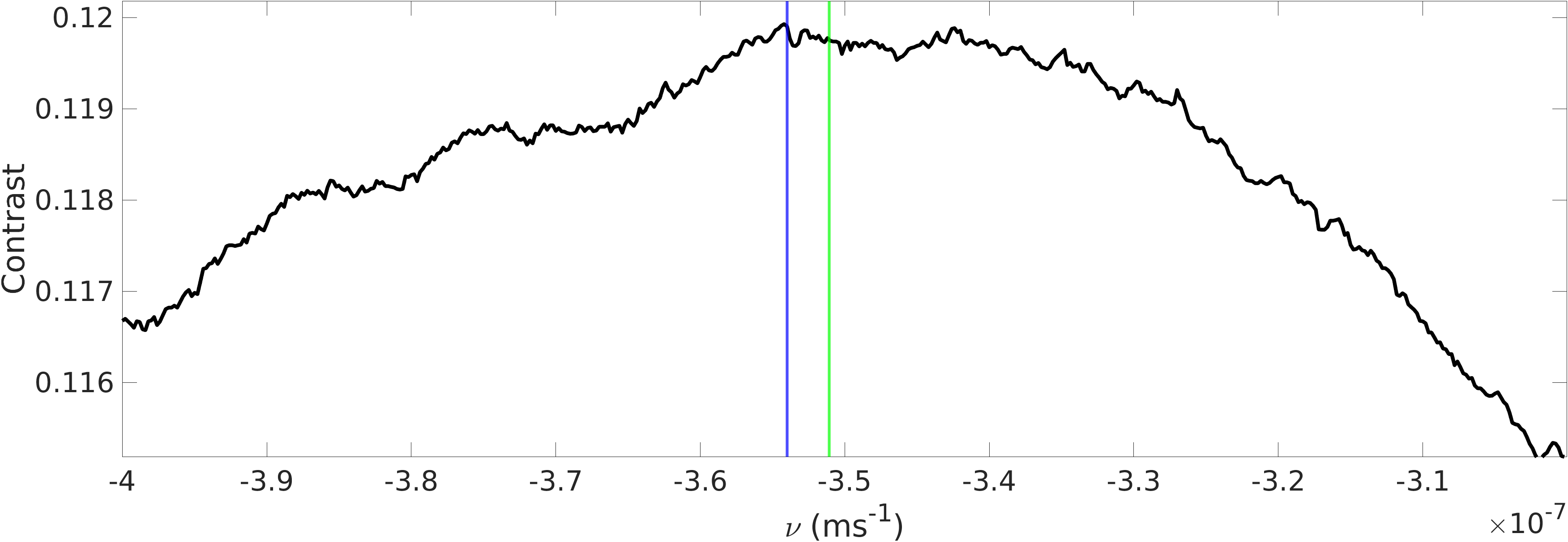
(a)

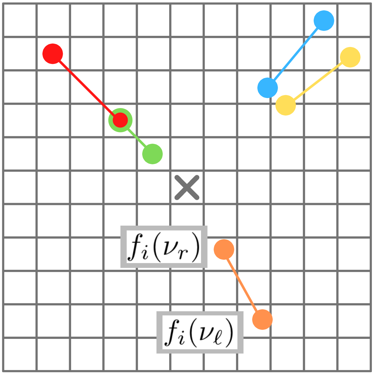
(b)

(c)

Figure 3: (a) Plot of the contrast function (14) for an event batch. Blue and green lines represent optimal and ground truth velocities respectively. Fig. 2(c) was produced by the optimal velocity. (b) Event lines $f_{i}(\nu_{\ell})\leftrightarrow f_{i}(\nu_{r})$ corresponding to five events (differentiated by colours) under velocity domain $\mathcal{V}=[\nu_{\ell},\nu_{r}]$. (c) Upper bound image $\bar{H}$ whose computation is GPU accelerated.

4.2 Contrast maximisation

To estimate $\nu$ from $\mathcal{E}=\{\mathbf{e}_{i}\}^{N}_{i=1}$, we define the event-based radial warp

$$f_{i}(\nu)=\begin{bmatrix}x_{i}\\ y_{i}\end{bmatrix}+\begin{bmatrix}\dfrac{x_{i}(Z_{0}+\nu t_{i})}{Z_{0}+\nu\tau}-x_{i},&\dfrac{y_{i}(Z_{0}+\nu t_{i})}{Z_{0}+\nu\tau}-y_{i}\end{bmatrix}^{T},$$ (12)

which is a specialisation of (9) by grounding $Z_{0}=1$ and warping $\mathbf{e}_{i}$ to the end $\tau$ of the duration of $\mathcal{E}$. The motion compensated image

$$H(\mathbf{u};\nu)=\sum_{i=1}^{N}\mathbb{I}(f_{i}(\nu)\textrm{ lies in pixel }\mathbf{u}),$$ (13)

accumulates events that are warped to the same pixel (note that we employ the discrete version of [29]). Intuitively, noisy events triggered by the same scene point will be warped by $f_{i}(\nu)$ to close-by pixels. This motivates contrast [18]

$$C(\nu)=\dfrac{1}{M}\sum_{\mathbf{u}}(H(\mathbf{u};\nu)-\mu(\nu))^{2},$$ (14)

of the motion compensated image as an objective function for estimating $\nu$, where $M$ is the number of pixels in the image, and $\mu(\nu)$ is the mean of $H(\mathbf{u};\nu)$. Fig. 3(a) illustrates the suitability of (14) for our aim. In particular, the true $\nu^{\ast}$ is very close to the maximiser of the contrast. Note that, following [18, 29] we do not utilise the event polarities, but they can be accommodated if desired.

4.3 Exact algorithm

As shown in Fig. 3(a), contrast (14) is non-convex and non-smooth. Liu et al. [29] demonstrated that maximising the contrast using approximate methods (e.g., via smoothing and gradient descent) could lead to bad local optima. Inspired by [29, 40], we developed a BnB method (Algorithm 1) to exactly maximise (14) over the domain $\mathcal{V}=[-1/\tau,0]$ of the vertical velocity $\nu$.

Starting with $\mathcal{V}$, Algorithm 1 iteratively splits and prunes $\mathcal{V}$ until the maximum contrast is found. For each subdomain, the upper bound $\bar{C}$ of the contrast over the subdomain (more details below) is computed and compared against the contrast of the current best estimate $\hat{\nu}$ to determine whether the subdomain can be discarded. The process continues until the difference between current best upper bound and the quality of $\hat{\nu}$ is less than a predefined threshold $\gamma$. Then, $\hat{\nu}$ is the globally optimal solution, up to $\gamma$. Given the velocity estimate from Algorithm 1, Sec. 4.1 shows how to retrieve the divergence.

Algorithm 1 Exact contrast maximisation for ventral velocity estimation.

1:Event batch $\mathcal{E}=\{\mathbf{e}_{i}\}_{i}^{N}$, batch duration $[0,\tau]$, convergence threshold $\gamma$.

2:Initialise $\mathcal{V}\leftarrow[-1/\tau,0]$, $\hat{\nu}\leftarrow$centre of $\mathcal{V}$.

3:$\textrm{Insert }\mathcal{V}\textrm{ into priority queue}~{}Q\textrm{ with priority }\bar{C}(\mathcal{V})$.

4:while $Q\textrm{ is not empty}$ do

5:     $\mathcal{V}\leftarrow\textrm{dequeue first item from }Q$.

6:     if $\bar{C}(\mathcal{V})-C(\hat{\nu})\leq\gamma$ then break.

7:     $\nu_{c}\leftarrow$ centre of $\mathcal{V}$.

8:     if $C(\nu_{c})\geq C(\hat{\nu})$ then $\hat{\nu}\leftarrow\nu_{c}$.

9:     Split $\mathcal{V}$ equally into 2 subdomains $\mathcal{V}_{1}$ and $\mathcal{V}_{2}$.

10:     for $s=1,2$ do

11:         if $\bar{C}(\mathcal{V}_{s})\geq C(\hat{\nu})$ then insert $\mathcal{V}_{s}$ into $Q$ with priority $\bar{C}(\mathcal{V}_{s})$.

12:     end for

13:end while

14:return $\hat{\nu}$.

4.3.1 Upper bound function

Following [29, Sec. 3], we use the general form

$$\bar{C}(\mathcal{V})=\frac{1}{M}\bar{S}(\mathcal{V})-\underline{\mu}(\mathcal{V})^{2},$$ (15)

as the upper bound for contrast, where the terms respectively satisfy

$$\bar{S}(\mathcal{V})\geq\max_{\nu\in\mathcal{V}}\sum_{\mathbf{u}}H(\mathbf{u};\nu)^{2}\;\;\;\;\textrm{and}\;\;\;\;\underline{\mu}(\mathcal{V})\leq\min_{\nu\in\mathcal{V}}\mu(\nu),$$ (16)

as well as equality in (16) when $\mathcal{V}$ is singleton. See [29, Sec. 3] on the validity of (15). For completeness, we also re-derive (15) in the supplementary material.

It remains to specify $\bar{S}$ and $\underline{\mu}$ for our ventral landing case. To this end, we define the upper bound image

$$\bar{H}(\mathbf{u};\mathcal{V})=\sum_{i=1}^{N}\mathbb{I}(f_{i}(\nu_{\ell})\leftrightarrow f_{i}(\nu_{r})\textrm{ intersects with pixel }\mathbf{u}),$$ (17)

where $\nu_{\ell}=\min(\mathcal{V})$ and $\nu_{r}=\max(\mathcal{V})$, and $f_{i}(\nu_{\ell})\leftrightarrow f_{i}(\nu_{r})$ is the line on the image that connects points $f_{i}(\nu_{\ell})$ and $f_{i}(\nu_{r})$; see Figs. 3(b) and 3(c). We can establish

$$\bar{H}(\mathbf{u};\mathcal{V})\geq H(\mathbf{u};\nu),\;\;\;\;\forall\nu\in\mathcal{V},$$ (18)

with equality achieved when $\mathcal{V}$ reaches a single point $\nu$ in the limit; see supplementary material for the proof. This motivates to construct

$$\bar{S}(\mathcal{V})=\sum_{\mathbf{u}}\bar{H}(\mathbf{u};\mathcal{V})^{2},$$ (19)

which satisfies the 1st condition in (16). For the 2nd term in (15), we use

$$\underline{\mu}(\mathcal{V})=\dfrac{1}{M}\sum_{i=1}^{N}\mathbb{I}(f_{i}(\nu_{\ell})\leftrightarrow f_{i}(\nu_{r})\textrm{ fully lies in the image plane)},$$ (20)

which satisfies the second condition in (16); see proof in supplementary material.

4.3.2 GPU acceleration

The main costs in Algorithm 1 are computing the contrast (14), contrast upper bound (15), and the line-pixel intersections (17). These routines are readily amenable to GPU acceleration via CUDA (this was suggested in [29], but no details or results were reported).

A key step is CUDA memory allocation to reduce the overheads of reallocating memory and copying data between CPU-GPU across the BnB iterations:

cudaMallocManaged(&event_image, )
cudaMallocManaged(&event_lines, )
cudaMalloc(&events, )
cudaMemcpy(&events, cpu_events, )

Summing all pixels (including with squaring the pixels), can be parallelised through the CUDA Thrust library:

sum_of_pixels = thrust::reduce(event_image_plane, )
sum_of_square_of_pixels = thrust::transform_reduce(
    event_image_plane, square<double>,plus<double>, )

Finally, the computation of all lines and line-pixel intersections can be parallelised through CUDA device functions:

get_upper_bound_lines <<< number_of_blocks, block_size >>>
Ψ    (events, event_lines, )
get_upper_bound_image <<< number_of_blocks, block_size >>>
Ψ    (event_lines, event_image_plane, )

Our CUDA acceleration (on an Nvidia GeForce RTX 2060) resulted in a runtime reduction of $80\%$ for the routines above, relative to pure CPU implementation.

4.4 Divergence estimation for event stream

The algorithm discussed in Sec. 4 can be used to estimate divergence for a single event batch $\mathcal{E}$. To estimate the time-varying divergence for the event stream $\mathcal{S}$, we incrementally take event batches from $\mathcal{S}$, and estimate the divergence of each batch as discrete samples of the continuous divergence value. In Sec. 6, we will report the batch sizes (which affect the sampling frequency) used in our work.

5 Ventral landing event dataset

Due to the lack of event datasets for ventral landing, we collected our own dataset to benchmark the methods. Our dataset consists of

• 1 simulated event sequence (SurfSim) of duration 47 seconds.

• 7 real event sequences observing 2D prints of landing surfaces (Surf2D-X, where X = 1 to 7) of duration 15 seconds each.

• 1 real event sequence observing the 3D print of a landing surface (Surf3D) of duration 15 seconds.

SurfSim was produced using v2e [25] to process a video that was graphically rendered using PANGU [4], of a camera undergoing pure ventral landing on a lunar-like surface (see Fig. 2).

Fig. 4 depicts our setup for recording the real event sequences. A UR5 robot arm was employed to execute a controlled linear trajectory towards horizontally facing 2D printed planetary surfaces (Mars, Mercury, etc.) and a 3D printed lunar surface (based on the lunar DEM from NASA/JAXA [3]). A Prophesee Gen 4 event camera and Intel RealSense depth sensor were attached to the end effector, while a work lamp provided lighting. Ground truth divergences at $33$ Hz were computed from velocities and depths retrieved from the robot arm and depth camera. Note that, despite using a robot arm, the real sequences do not fully obey the ventral landing assumptions, due to the surfaces not being strictly fronto-parallel to the camera, and the 3D surface not being planar.

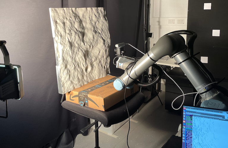
(a)

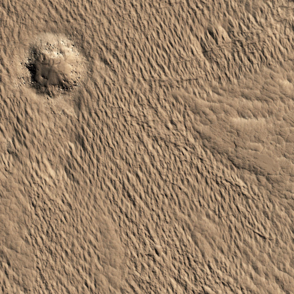
(b)

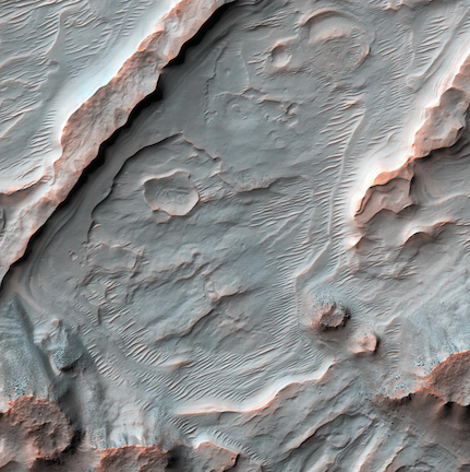
(c)

Figure 4: (a) Our setup for recording real event data under (approximate) ventral landing, shown here with the 3D printed lunar surface. Note the only approximately fronto-parallel surface. (b)(c) [33, 34] Two of the planetary surface images that were 2D printed. See supplementary material for more details.

6 Results

We tested our method, exact contrast maximisation for event-based divergence estimation (ECMD), on the dataset described in Sec. 5. We compared against:

• Local plane fitting (PF) method [41];

• 2D centroid tracking (CT) method [47];

• Learning-based dense OF method (E-RAFT) [20]; and

• Tracking and grid search-based OF method (SOFAS) [51, 53].

Only PF and CT were aimed at divergence estimation, whereas SOFAS and E-RAFT are general OF methods. While there are other event-based OF methods, e.g., [6, 18, 19, 30, 37, 58], our list includes the main categories of heuristic, optimisation and learning methods which had publicly available implementations.

6.0.1 Preprocessing

All event sequences were subject to radial undistortion and hot pixel removal. Two versions of the data were also produced:

• Full resolution: The original data collected for Surf2D-X and Surf3D by our Prophesee Gen 4 event camera ($1280$x$760$ pixels) and simulated data for SurfSim ($512$x$512$ pixels), with only the processing above.

• Resized and resampled: The effective image resolution of the camera was resized (by scaling the image coordinates of the events) to $160$x$90$ pixels for Surf2D-X and Surf3D, and $64$x$64$ pixels for SurfSim. The size of each event batch was also reduced by $75\%$ by random sampling.

6.0.2 Implementation and tuning

For ECMD, the convergence threshold $\gamma$ (see Algorithm 1) was set to 0.025, and an event batch duration of $0.5$ s was used. For PF, we used the implementation available at [5]. There were 16 hyperparameters that influence the estimated divergence in nontrivial ways, thus we used the default values. Note that PF is an asynchronous algorithm, thus its temporal sampling frequency is not directly comparable to the other methods. We used our own implementation of CT. The two main parameters were the temporal memory and batch duration, which we tuned to to $0.3$ s and $0.1$ s for best performance. For SOFAS, we used the implementation available at [2] with batch duration of $0.5$ s. For E-RAFT, we used the implementation available at [1]. As there was no network training code available, we used the provided DSEC pre-trained network. E-RAFT was configured to output OF estimates every $0.5$ s.

All methods were executed on a standard machine with an Core i7 CPU and RTX 2060 GPU. See supplementary material for more implementation details.

6.0.3 Converting OF to divergence

For E-RAFT and SOFAS, the divergence for each event batch was calculated from the OF estimates by finding the rate of perceived expansion of the OF vectors, as defined in [47] as

$$D=\dfrac{1}{P\tau}\sum_{k=1}^{P}\left[1-\dfrac{\lVert FOE+\mathbf{p}_{k}+\tau\mathbf{v}_{k}\rVert}{\lVert FOE+\mathbf{p}_{k}|\rVert}\right],$$ (21)

where $P$ is the number of OF vectors, $\mathbf{v}_{k}$ is the $k$-th OF vector at corresponding pixel location $\mathbf{p}_{k}$, and $\tau$ is the duration of the event batch.

6.0.4 Comparison metrics

For each method, we recorded:

• Divergence error: The absolute error (in $\%$) between the estimated divergence and closest-in-time ground truth divergence for each event batch.

• Runtime: The runtime of the method on the event batch.

Since the methods were operated at different temporal resolutions for best performance, to allow comparisons we report results at $0.5$ s time resolution, by taking the average divergence estimate of methods that operated at finer time scales (specifically PF at $0.01$ s and CT at $0.3$ s) over $0.5$ s windows.

6.1 Qualitative results

Fig. 5 shows motion compensated event images from the estimated $\nu$ across all methods in Sec. 6, including event images produced under ground truth (GT) $\nu$, and when $\nu=0$ (Zero). In these examples, ECMD returned the highest image contrast (close to the contrast of GT).

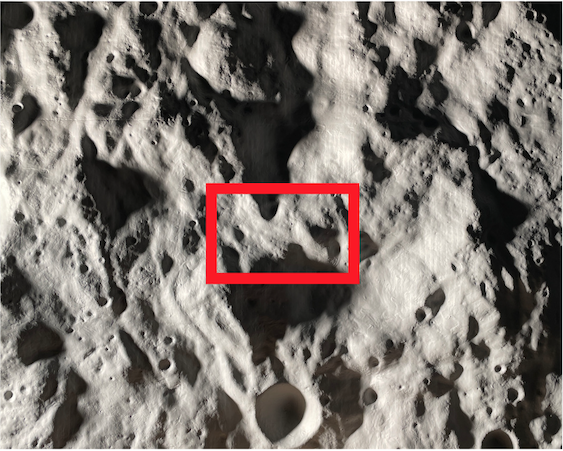
(a) Surf2D-1

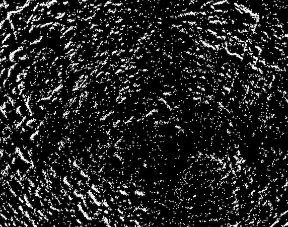
(b) GT (0.033)

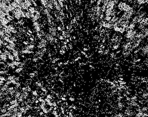
(c) Zero (0.026)

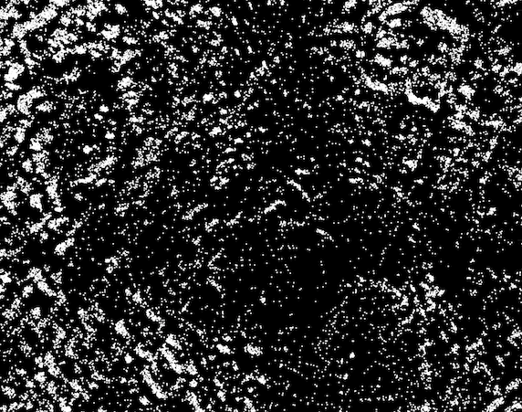
(d) PF (0.028)

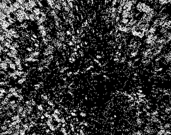
(e) CT (0.026)

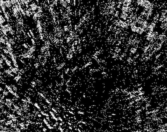
(f) E-RAFT (0.024)

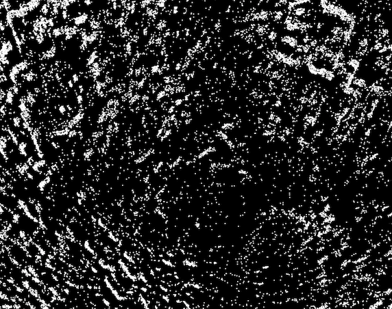
(g) SOFAS (0.027)

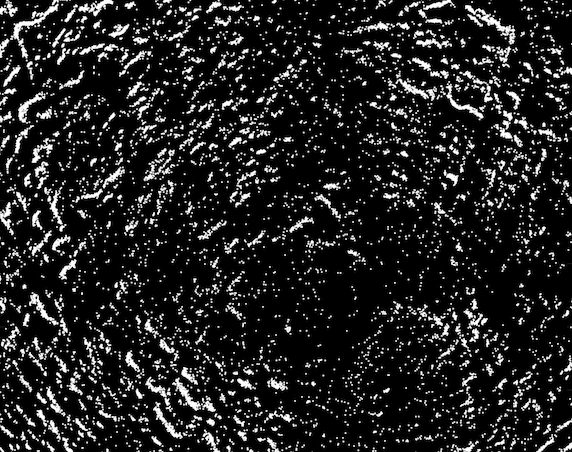
(h) ECMD (0.033)

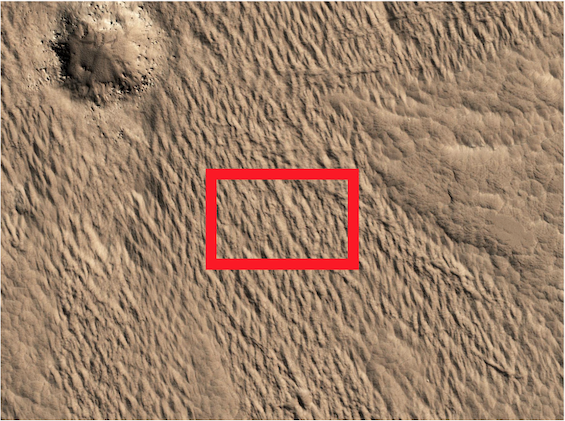
(i) Surf2D-6

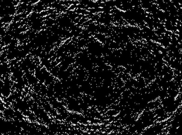
(j) GT (1.82)

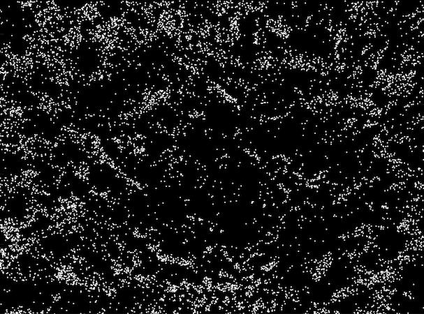
(k) Zero (1.05)

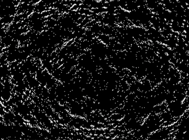
(l) PF (1.8)

(m) CT (1.64)

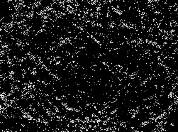
(n) E-RAFT (1.21)

(o) SOFAS (1.64)

(p) ECMD (1.82)

Figure 5: (b)-(h) Flow-compensated event images produced for an event batch (full resolution) from Surf2D-1. (j)-(p) Flow-compensated event images produced for an event batch (resized and resampled) from Surf2D-6 [33]. GT = Ground truth. Zero = No warp. Numbers in parentheses are the contrast values (14).

6.2 Quantitative results on full resolution sequences

Fig. 6 (top row) plots the estimated divergence for all methods across 3 of the full resolution event sequences; see supplementary material for the rest of the sequences. Observe that ECMD generally tracked the ground truth divergence well and was the most stable method. The estimates of the other methods were either inaccurate or quite erratic. A common failure point was towards the end of SurfSim; this was when the camera was very close to the surface and the limited resolution of the rendered image did not generate informative events.

Table 1 (top) provides average divergence errors and runtimes. Values of the former reflect the trends in Fig. 6; across all sequences, ECMD committed the least error relative to the ground truth. The results suggest that, although ECMD was based upon a pure vertical landing assumption, the method was not greatly affected by violations of the assumption in the real event sequences.

While PF and E-RAFT were more efficient (up to one order of magnitude faster than ECMD), their estimates were rather inaccurate. Despite GPU acceleration, the runtime of ECMD was longer than event batch duration. We will present results on the resized and resampled sequences next.

Table 1: Divergence estimation results (error and runtime) on event sequences. The final column contains the average error and runtime across all sequences.

Full resolution event sequences
Dataset		Surf-Sim	Surf 2D-1	Surf 2D-2	Surf 2D-3	Surf 2D-4	Surf 2D-5	Surf 2D-6	Surf 2D-7	Surf-3D	Avg.
Absolute average error per event batch(%)	ECMD	8.34	13.48	7.41	6.11	12.19	10.41	5.12	3.72	12.90	8.85
	PF	37.78	39.11	44.79	44.42	41.19	42.19	43.42	44.03	25.23	40.24
	CT	44.33	43.86	50.27	42.96	50.07	72.80	53.73	60.30	45.85	51.57
	E-RAFT	46.27	50.79	44.81	44.75	41.12	29.90	53.53	49.19	21.82	43.46
	SOFAS	819.33	24.85	24.65	23.63	30.67	34.80	37.05	30.88	71.54	121.93
Average runtime per event batch(s)	ECMD	7.99	6.84	6.95	6.50	5.85	7.62	6.02	3.01	2.36	5.90
	PF	0.21	0.22	0.23	0.30	0.18	0.28	0.22	0.14	0.13	0.21
	CT	35.12	31.58	35.46	41.67	28.48	48.49	42.17	21.43	20.98	33.93
	E-RAFT	0.24	0.25	0.25	0.24	0.25	0.25	0.24	0.25	0.24	0.25
	SOFAS	57.80	61.46	66.43	65.79	55.62	66.23	59.32	13.27	35.83	53.53

Resized and resampled event sequences
Dataset		Surf-Sim	Surf 2D-1	Surf 2D-2	Surf 2D-3	Surf 2D-4	Surf 2D-5	Surf 2D-6	Surf 2D-7	Surf-3D	Avg.
Absolute average error per event batch(%)	ECMD	18.65	18.86	10.33	7.36	14.45	12.28	7.41	4.25	11.68	11.70
	PF	146.76	58.66	32.79	50.49	52.66	43.80	57.36	30.61	31.64	56.09
	CT	102.20	143.99	51.83	73.35	40.57	81.72	89.83	96.80	43.47	80.42
	E-RAFT	47.40	86.40	72.31	88.62	81.67	71.87	91.26	66.79	21.19	69.72
	SOFAS	1688.21	60.10	50.49	56.29	67.73	47.87	24.42	42.98	63.51	233.51
Average runtime per event batch(s)	ECMD	0.20	0.31	0.29	0.32	0.34	0.34	0.30	0.28	0.23	0.29
	PF	0.12	0.10	0.10	0.10	0.17	0.07	0.12	0.10	0.06	0.10
	CT	7.81	20.65	22.09	30.59	32.79	13.99	27.38	11.63	15.33	20.25
	E-RAFT	0.24	0.24	0.25	0.24	0.24	0.25	0.25	0.25	0.24	0.24
	SOFAS	6.14	36.18	39.06	39.54	38.67	34.63	40.13	36.96	25.27	32.95

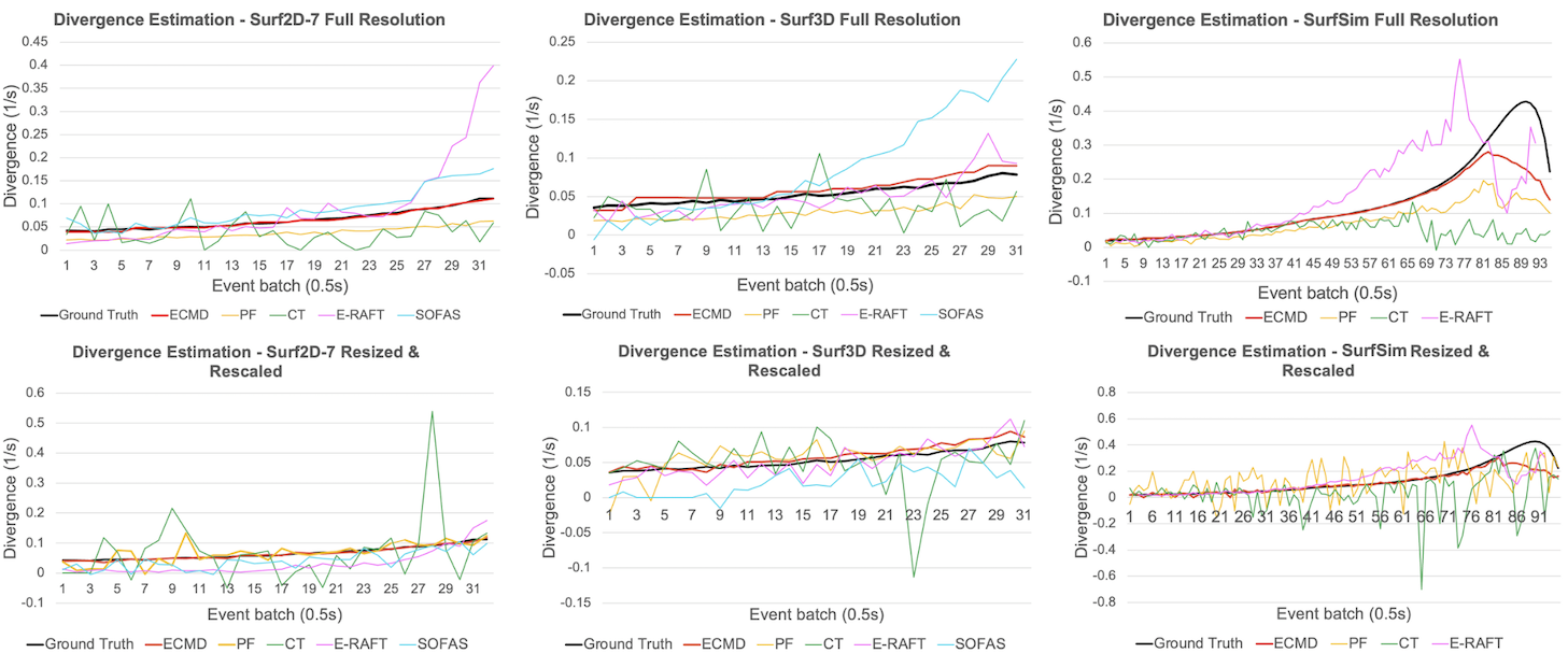
Figure 6: Divergence estimates from the methods described in Sec. 6 for datasets Surf2D-7, Surf3D, and SurfSim. (Top row) Full resolution sequences. (Bottom row) Resized and resampled sequences. Note that SOFAS was not plotted for SurfSim since the divergence estimates were too innacurate (see Table 1).

6.3 Quantitative results on resized and resampled sequences

Fig. 6 (bottom row) plots the estimated divergence for all methods across 3 of the resized and resampled event sequences; see supplementary material for the rest of the sequences. Table 1 (bottom) provides average errors and runtimes.

The results show that the accuracy of all methods generally deteriorated due to the lower image resolution and event subsampling. However, the impact on the accuracy of ECMD has been relatively small, with a difference in average error of within $3\%$ from the full resolution results. Though PF was still the fastest method, the average runtime of ECMD has reduced by about $95\%$. The average runtime of ECMD was $0.29$ s, which was below the batch duration.

7 Conclusions and future work

This paper proposes exact contrast maximisation for event-based divergence estimation (ECMD) for guiding ventral descent. Compared to other divergence and OF methods, ECMD demonstrated stable and accurate divergence estimates across our ventral landing dataset. Violations to the ECMD assumption on a pure ventral landing did not greatly affect the divergence estimates. Through GPU acceleration and downsampling, ECMD achieved competitive runtimes.

Future work includes integrating ECMD into a closed loop system [41, 47], and comparing GPU-enabled ECMD to SNN event-based OF methods.

8 Acknowledgements

Sofia Mcleod was supported by the Australian Government RTP Scholarship. Tat-Jun Chin is SmartSat CRC Professorial Chair of Sentient Satellites.

References

- [1] E-raft: Dense optical flow from event cameras. https://github.com/uzh-rpg/E-RAFT, accessed: 2022-02-24
- [2] Event contrast maximization library. https://github.com/TimoStoff/events_contrast_maximization, accessed: 2022-02-27
- [3] Moon lro lola - selene kaguya tc dem merge 60n60s 59m v1. https://astrogeology.usgs.gov/search/map/Moon/LRO/LOLA/Lunar_LRO_LOLAKaguya_DEMmerge_60N60S_512ppd, accessed: 2021-06-24
- [4] Planet and asteroid natural scene generation utility product website. https://pangu.software/, accessed: 2022-01-26
- [5] Vertical landing for micro air vehicles using event-based optical flow dataset. https://dataverse.nl/dataset.xhtml?persistentId=hdl:10411/FBKJFH, accessed: 2022-01-31
- [6] Almatrafi, M., Baldwin, R., Aizawa, K., Hirakawa, K.: Distance surface for Event-Based optical flow. IEEE Transactions on Pattern Analysis and Machine Intelligence 42(7), 1547–1556 (2020)
- [7] Bardow, P., Davison, A.J., Leutenegger, S.: Simultaneous optical flow and intensity estimation from an event camera. In: Proceedings of the IEEE Conference on Computer Vision and Pattern Recognition. pp. 884–892 (2016)
- [8] Benosman, R., Clercq, C., Lagorce, X., Ieng, S.H., Bartolozzi, C.: Event-based visual flow. IEEE Transactions on Neural Networks and Learning Systems 25(2), 407–417 (2014)
- [9] Benosman, R., Ieng, S.H., Clercq, C., Bartolozzi, C., Srinivasan, M.: Asynchronous frameless event-based optical flow. Neural Networks 27, 32–37 (2012)
- [10] Brandli, C., Berner, R., Yang, M., Liu, S.C., Delbruck, T.: A 240 180 130 db 3 µs latency global shutter spatiotemporal vision sensor. IEEE Journal of Solid-State Circuits 49(10), 2333–2341 (2014)
- [11] Chin, T.J., Bagchi, S., Eriksson, A., van Schaik, A.: Star tracking using an event camera. IEEE/CVF Conference on Computer Vision and Pattern Recognition Workshops (CVPRW) (2019)
- [12] Clady, X., Clercq, C., Ieng, S.H., Houseini, F., Randazzo, M., Natale, L., Bartolozzi, C., Benosman, R.: Asynchronous visual event-based time-to-contact. Frontiers in neuroscience 8, 9 (2014)
- [13] Dinaux, R., Wessendorp, N., Dupeyroux, J., Croon, G.C.H.E.d.: FAITH: Fast iterative Half-Plane focus of expansion estimation using optic flow. IEEE Robotics and Automation Letters 6(4), 7627–7634 (2021)
- [14] Ding, Z., Zhao, R., Zhang, J., Gao, T., Xiong, R., Yu, Z., Huang, T.: Spatio-Temporal recurrent networks for Event-Based optical flow estimation. AAAI Conference on Artificial Intelligence pp. 1–13 (2021)
- [15] Falanga, D., Kleber, K., Scaramuzza, D.: Dynamic obstacle avoidance for quadrotors with event cameras. Sci Robot 5(40) (2020)
- [16] Forsyth, D., Ponce, J.: Computer vision: A modern approach. Prentice hall (2011)
- [17] Fry, S.N.: Experimental approaches toward a functional understanding of insect flight control. In: Floreano, D., Zufferey, J.C., Srinivasan, M.V., Ellington, C. (eds.) Flying Insects and Robots, pp. 1–13. Springer Berlin Heidelberg, Berlin, Heidelberg (2010)
- [18] Gallego, G., Rebecq, H., Scaramuzza, D.: A unifying contrast maximization framework for event cameras, with applications to motion, depth, and optical flow estimation. In: 2018 IEEE/CVF Conference on Computer Vision and Pattern Recognition. pp. 3867–3876 (2018)
- [19] Gehrig, D., Loquercio, A., Derpanis, K.G., Scaramuzza, D.: End-to-end learning of representations for asynchronous event-based data. In: Proceedings of the IEEE/CVF International Conference on Computer Vision. pp. 5633–5643 (2019)
- [20] Gehrig, M., Millhäusler, M., Gehrig, D., Scaramuzza, D.: E-RAFT: Dense optical flow from event cameras. In: 2021 International Conference on 3D Vision (3DV). pp. 197–206 (2021)
- [21] Gómez Eguíluz, A., Rodríguez-Gómez, J.P., Martínez-de Dios, J.R., Ollero, A.: Asynchronous event-based line tracking for Time-to-Contact maneuvers in UAS. In: 2020 IEEE/RSJ International Conference on Intelligent Robots and Systems (IROS). pp. 5978–5985 (2020)
- [22] Haessig, G., Cassidy, A., Alvarez, R., Benosman, R., Orchard, G.: Spiking optical flow for Event-Based sensors using IBM’s TrueNorth neurosynaptic system. IEEE Transactions on Biomedical Circuits and Systems 12(4), 860–870 (2018)
- [23] Hagenaars, J.J., Paredes-Vallés, F., de Croon, G.C.H.E.: Self-Supervised learning of Event-Based optical flow with spiking neural networks. Neural Information Processing Systems (Oct 2021)
- [24] Horst, R., Hoang, T.: Global Optimization: Deterministic Approaches. Springer-Verlag (1996)
- [25] Hu, Y., Liu, S.C., Delbruck, T.: v2e: From video frames to realistic DVS events. 2021 IEEE/CVF Conference on Computer Vision and Pattern Recognition Workshops (CVPRW) (2021)
- [26] Intel: Beyond today’s ai, https://www.intel.com.au/content/www/au/en/research/neuromorphic-computing.html
- [27] Lee, C., Kosta, A.K., Zhu, A.Z., Chaney, K., Daniilidis, K., Roy, K.: Spike-FlowNet: Event-Based optical flow estimation with Energy-Efficient hybrid neural networks. In: ECCV. pp. 366–382. Springer International Publishing (2020)
- [28] Lichtsteiner, P., Posch, C., Delbruck, T.: A 128128 120 db 15 s latency asynchronous temporal contrast vision sensor. IEEE Journal of Solid-State Circuits 43(2), 566–576 (2008)
- [29] Liu, D., Parra, A., Chin, T.J.: Globally optimal contrast maximisation for event-based motion estimation. In: Proceedings of the IEEE/CVF Conference on Computer Vision and Pattern Recognition. pp. 6349–6358 (2020)
- [30] Liu, M., Delbruck, T.: Adaptive time-slice block-matching optical flow algorithm for dynamic vision sensors. British Machine Vision Conference (BMVC) (2018)
- [31] Lucas, B.D., Kanade, T.: An iterative image registration technique with an application to stereo vision. International Joint Conference on Artificial Intelligence pp. 674–679 (1981)
- [32] Mueggler, E., Huber, B., Scaramuzza, D.: Event-based, 6-DOF pose tracking for high-speed maneuvers. In: 2014 IEEE/RSJ International Conference on Intelligent Robots and Systems. pp. 2761–2768 (2014)
- [33] NASA/JPL-Caltech/Univ. of Arizona: Decoding a geological message (2017), https://www.nasa.gov/sites/default/files/thumbnails/image/pia21759.jpg
- [34] NASA/JPL-Caltech/Univ. of Arizona: Big fans (2018), https://www.nasa.gov/image-feature/jpl/pia22332/big-fans
- [35] Orchard, G., Bartolozzi, C., Indiveri, G.: Applying neuromorphic vision sensors to planetary landing tasks. In: IEEE Biomedical Circuits and Systems Conference. pp. 201–204 (2009)
- [36] Orchard, G., Benosman, R., Etienne-Cummings, R., Thakor, N.V.: A spiking neural network architecture for visual motion estimation. In: IEEE Biomedical Circuits and Systems Conference (BioCAS). pp. 298–301 (2013)
- [37] Pan, L., Liu, M., Hartley, R.: Single image optical flow estimation with an event camera. In: IEEE/CVF Conference on Computer Vision and Pattern Recognition (CVPR). pp. 1669–1678 (2020)
- [38] Paredes-Vallés, F., de Croon, G.C.H.E.: Back to event basics: Self-Supervised learning of image reconstruction for event cameras via photometric constancy. 2021 IEEE/CVF Conference on Computer Vision and Pattern Recognition (CVPR) (2021)
- [39] Paredes-Vallés, F., Scheper, K.Y.W., de Croon, G.C.H.E.: Unsupervised learning of a hierarchical spiking neural network for optical flow estimation: From events to global motion perception. IEEE Trans. Pattern Anal. Mach. Intell. 42(8), 2051–2064 (2020)
- [40] Peng, X., Wang, Y., Gao, L., Kneip, L.: Globally-Optimal event camera motion estimation. In: Computer Vision – ECCV 2020. pp. 51–67. Springer International Publishing (2020)
- [41] Pijnacker Hordijk, B.J., Scheper, K.Y.W., de Croon, G.C.H.E.: Vertical landing for micro air vehicles using event-based optical flow. J. field robot. 35(1), 69–90 (2018)
- [42] Posch, C., Matolin, D., Wohlgenannt, R.: A QVGA 143 db dynamic range Frame-Free PWM image sensor with lossless Pixel-Level video compression and Time-Domain CDS. IEEE J. Solid-State Circuits 46(1), 259–275 (2011)
- [43] Rebecq, H., Ranftl, R., Koltun, V., Scaramuzza, D.: Events-To-Video: Bringing modern computer vision to event cameras. 2019 IEEE/CVF Conference on Computer Vision and Pattern Recognition (CVPR) (2019)
- [44] Rebecq, H., Ranftl, R., Koltun, V., Scaramuzza, D.: High speed and high dynamic range video with an event camera. IEEE Transactions on Pattern Analysis and Machine Intelligence 43(6), 1964–1980 (2019)
- [45] Sanket, N.J., Parameshwara, C.M., Singh, C.D., Kuruttukulam, A.V., Fermüller, C., Scaramuzza, D., Aloimonos, Y.: EVDodgeNet: Deep dynamic obstacle dodging with event cameras. In: 2020 IEEE International Conference on Robotics and Automation (ICRA). pp. 10651–10657 (2020)
- [46] Scheerlinck, C., Rebecq, H., Gehrig, D., Barnes, N., Mahony, R., Scaramuzza, D.: Fast image reconstruction with an event camera. In: Proceedings of the IEEE/CVF Winter Conference on Applications of Computer Vision. pp. 156–163 (2020)
- [47] Sikorski, O., Izzo, D., Meoni, G.: Event-Based spacecraft landing using Time-To-Contact. In: Proceedings of the IEEE/CVF Conference on Computer Vision and Pattern Recognition. pp. 1941–1950 (2021)
- [48] Srinivasan, M., Zhang, S., Lehrer, M., Collett, T.: Honeybee navigation en route to the goal: visual flight control and odometry. The Journal of Experimental Biology 199(Pt 1), 237–244 (1996)
- [49] Srinivasan, M.V.: Honeybees as a model for the study of visually guided flight,navigation, and biologically inspired robotics. Physical Review 91, 413–406 (2011)
- [50] Srinivasan, M.V., Thurrowgood, S., Soccol, D.: From visual guidance in flying insects to autonomous aerial vehicles. In: Floreano, D., Zufferey, J.C., Srinivasan, M.V., Ellington, C. (eds.) Flying Insects and Robots, pp. 15–28. Springer Berlin Heidelberg, Berlin, Heidelberg (2010)
- [51] Stoffregen, T., Kleeman, L.: Simultaneous optical flow and segmentation (SOFAS) using dynamic vision sensor. In: Australasian Conference on Robotics and Automation (2018)
- [52] Stoffregen, T., Gallego, G., Drummond, T., Kleeman, L., Scaramuzza, D.: Event-based motion segmentation by motion compensation. International Conference on Computer Vision pp. 7243–7252 (2019)
- [53] Stoffregen, T., Kleeman, L.: Event cameras, contrast maximization and reward functions: an analysis. In: IEEE/CVF Conference on Computer Vision and Pattern Recognition. pp. 12300–12308 (2019)
- [54] Tammero, L.F., Dickinson, M.H.: The influence of visual landscape on the free flight behavior of the fruit fly drosophila melanogaster. J. Exp. Biol. 205(Pt 3), 327–343 (2002)
- [55] Valette, F., Ruffier, F., Viollet, S., Seidl, T.: Biomimetic optic flow sensing applied to a lunar landing scenario. In: 2010 IEEE International Conference on Robotics and Automation. pp. 2253–2260 (2010)
- [56] Vasco Medici, Garrick Orchard, Stefan Ammann, Giacomo Indiveri, Steven N. Fry: Neuromorphic computation of optic flow data. Tech. rep., European Space Agency, Advanced Concepts Team (2010)
- [57] Vidal, A.R., Rebecq, H., Horstschaefer, T., Scaramuzza, D.: Ultimate SLAM? combining events, images, and IMU for robust visual SLAM in HDR and High-Speed scenarios. IEEE Robotics and Automation Letters 3(2), 994–1001 (2018)
- [58] Ye, C., Mitrokhin, A., Fermüller, C., Yorke, J.A., Aloimonos, Y.: Unsupervised learning of dense optical flow, depth and egomotion with Event-Based sensors. In: 2020 IEEE/RSJ International Conference on Intelligent Robots and Systems (IROS). pp. 5831–5838 (2020)
- [59] Zhou, Y., Gallego, G., Lu, X., Liu, S., Shen, S.: Event-Based motion segmentation with Spatio-Temporal graph cuts. IEEE Transactions on Neural Networks and Learning Systems PP (2020)
- [60] Zhu, A.Z., Yuan, L., Chaney, K., Daniilidis, K.: EV-FlowNet: Self-Supervised optical flow estimation for event-based cameras. Robotics: Science and Systems (2018)
- [61] Zhu, A.Z., Yuan, L., Chaney, K., Daniilidis, K.: Unsupervised event-based learning of optical flow, depth, and egomotion. In: Proceedings of the IEEE/CVF Conference on Computer Vision and Pattern Recognition. pp. 989–997. openaccess.thecvf.com (2019)