On polynomial-time solvability of combinatorial Markov random fields

Abstract.

The problem of inferring Markov random fields (MRFs) with a sparsity or robustness prior can be naturally modeled as a mixed-integer program. This motivates us to study a general class of convex submodular optimization problems with indicator variables, which we show to be polynomially solvable in this paper. The key insight is that, possibly after a suitable reformulation, indicator constraints preserve submodularity. Fast computations of the associated Lovász extensions are also discussed under certain smoothness conditions, and can be implemented using only linear-algebraic operations in the case of quadratic objectives.

Keywords. Submodularity, mixed-integer optimization, Markov random fields, sparsity, robustness

September 2022

1. Introduction

Markov random fields (MRFs) are popular graphical models pervasively used to represent spatio-temporal processes. They are defined on an undirected graph $\mathcal{G}=(\mathcal{V},\mathcal{E})$, where there is random variable $X_{i}$ associated with each vertex $i\in\mathcal{V}$. Each edge $[i,j]\in\mathcal{E}$ represents the a relationship between the variables at their respective nodes $i$ and $j$; usually, these two variables should take similar values. Moreover, variables not connected by an edge are conditionally independent given realizations of all other variables. In the MRF inference problems we consider, noisy realizations $\{a_{i}\}_{i\in\mathcal{V}}$ of the random variables $\bm{X}$ are observed, and the goal is to infer the true values of $\bm{X}$. Figure 1 provides a depiction of this problem for three commonly-used structures of MRFs.

(a) 1D

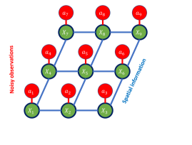
(b) 2D

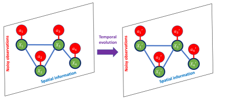
(c) 3D

Figure 1. Common topologies of MRFs, modeling spatial (blue) and temporal (purple) relationships. The true values of random variables $\bm{X}$ (green) are not observed directly, and need to be inferred from the noisy observations $\bm{a}$ (red).

One-dimensional MRFs as depicted in Figure 1 (A) are fundamental building blocks in time series analysis and signal processing [3, 34, 44, 45, 52, 53]. They are typically used to model the evolution of a given process or signal over time. Two-dimensional MRFs as depicted in Figure 1 (B) arise pervasively in image denoising [13, 14, 31, 32, 40] and computer vision [25]. Each variable $X_{i}$ encodes the “true” value of a pixel in an image, and edges encode the belief that adjacent pixels tend to have similar values. Three-dimensional MRFs as depicted in Figure 1 (C) are used to model spatio-temporal processes [22]. They are used in epidiomology [12, 39, 46] for example to track the spread of a disease over time. In addition, MRFs over general graphs airse in semiconductor manufacturing [21, 33], bioinformatics [20], criminology [41], spam detection [35], among other applications.

Maximum a posteriori estimates of the values of $\bm{X}$ can often be obtained as optimal solutions of the (continuous) MRF problem [31]

$$\operatorname*{\mathbf{minimize}}\limits_{\bm{\ell}\leq\bm{x}\leq\bm{u}}\;\sum_{i\in\mathcal{V}}h_{i}(x_{i}-a_{i})+\sum_{[i,j]\in\mathcal{E}}g_{ij}(x_{i}-x_{j}),$$ (1)

where $h_{i}:\mathbb{R}\to\mathbb{R}_{+}$ and $g_{ij}:\mathbb{R}\to\mathbb{R}_{+}$ are appropriate convex nonnegative one-dimensional functions such that $h_{i}(0)=g_{ij}(0)=0$, and $\bm{\ell}\leq\bm{u}$ are (possibly infinite) lower and upper bounds, respectively, on the values of $\bm{X}$. Functions $h_{i}$ and $g_{ij}$ are chosen depending on the prior distribution of the random variables and noise. Typically, functions $h_{i}$ are quadratic, corresponding to cases with Gaussian noise. The most common choices for functions $g_{ij}$ are absolute value functions $g_{ij}(x_{i}-x_{j})=c_{ij}|x_{i}-x_{j}|$ with $c_{ij}\geq 0$, popular in statistics and signal processing [57, 18] and referred to as total variation denoising problems, and quadratic functions $g_{ij}(x_{i}-x_{j})=c_{ij}(x_{i}-x_{j})^{2}$, in which case the graphical model is a Gaussian MRF (GMRF) and also corresponds to a Besag model [10, 11].

Clearly, problem (1) is convex and can be solved using standard tools in the convex optimization literature. Specialized algorithms have also been proposed [1, 31], whose complexity is strongly polynomial for the special cases of total variation and Besag models (see also [32] and the references therein). In this paper, we study two combinatorial extensions of (1). The first extension corresponds to the situation where $\bm{X}$ is sparse or, more generally, is assumed to take a baseline value (e.g., corresponding to the background of an image or the absence of a disease) in most of its coordinates. In such cases, statistical theory calls for the imposition of an $\ell_{0}$ regularization to penalize variables that differ from the baseline value. The second extension corresponds to the situation where the noisy observations are corrupted by a few but potentially gross outliers. In such cases, statistical theory calls for the simultaneous removal of data identified as corrupted and solution of (1). Both extensions involve combinatorial decisions: which random variables differ from the baseline value, and which datapoints should be discarded.

It is well known that linear regression, one of the simplest statistical estimation methods, becomes NP-hard with the inclusion of either sparsity [48] or robustness [7] as described above. Thus, approaches in the literature resort to approximations of the combinatorial problems, heuristics, or expensive mixed-integer optimization approaches to solve the exact problems. In this paper we show that for the case of (1), the aforementioned combinatorial extensions can in fact be solved in polynomial time by a reduction to submodular minimization. We point out that an immediate application of submodular minimization techniques [50] results in runtimes of $\mathcal{O}(n^{5}\cdot\mathsf{OE})$, where $\mathsf{OE}$ is the complexity of solving problem (1) – resulting for example in strongly polynomial but impractical complexities of $\mathcal{O}(n^{8})$ for the case of total variation and Besag models, but those runtimes can likely be improved (we present such an improvement in this paper). Indeed, the discovery of a (strongly) polynomial time algorithm for a problem has typically been closely followed by highly efficient methods.

Outline

In §2 we discuss the necessary preliminaries for the paper and introduce mixed-integer optimization formulations of the problems we consider. In §3 we show that the aforementioned variants of (1) can be reduced to the minimization of a submodular set function –a class of problems which admits polynomial time algorithms [37, 38]. In §4 we describe parametric procedures that can be used to improve the complexity of submodular minimization algorithms for this class of problems. Finally, in §5 we conclude the paper.

2. Preliminaries

In this section we give explicit mixed-integer optimization (MIO) formulations of the problems under consideration, and review the concepts and literature relevant to the paper. First, we introduce the notation used throughout the paper.

Notation

We use bold symbols to denote vectors and matrices. Given $n\in\mathbb{Z}_{++}$, we let $[n]\stackrel{{\scriptstyle\mathclap{\text{\tiny def}}}}{{=}}\{1,\dots,n\}$. We denote the vector of all zeros by $\bm{0}$ and the vector of ones by $\operatorname*{\textbf{1}}$ (whose dimensions can be inferred from the context). Given a set $\mathcal{S}\subseteq\mathbb{R}^{n}$, we let $\bm{\operatorname*{\textbf{1}}}_{\mathcal{S}}\in\{0,1\}^{n}$ be the indicator vector of $\mathcal{S}$, i.e., $(\bm{\operatorname*{\textbf{1}}}_{\mathcal{S}})_{i}=1$ if $i\in\mathcal{S}$ and is zero otherwise. Given $i\in[n]$, we also let $\bm{e^{i}}$ be the $i$-th basis vector of $\mathbb{R}^{n}$. Given two vectors $\bm{y^{1}}$ and $\bm{y^{2}}\in\mathbb{R}^{n}$, define the meet $\bm{y^{1}}\operatorname{\wedge}\bm{y^{2}}\in\mathbb{R}^{n}$ and the join $\bm{y^{1}}\operatorname{\vee}\bm{y^{2}}\in\mathbb{R}^{n}$ to be the component-wise minimum and maximum of $\bm{y^{1}}$ and $\bm{y^{2}}$, respectively; we also define $\bm{y^{1}}\circ\bm{y^{2}}$ as the Hadamard (entrywise) product. By above notations, a set $\mathcal{L}\subseteq\mathbb{R}^{n}$ is called a lattice if any $\bm{y}^{1},\bm{y}^{2}\in\mathcal{L}$ implies that $\bm{y}^{1}\operatorname{\vee}\bm{y}^{2}$ and $\bm{y}^{1}\operatorname{\wedge}\bm{y}^{2}$ belong to $\mathcal{L}$. A function $f:\mathbb{R}^{n}\to\mathbb{R}$ is submodular over a lattice $\mathcal{L}$ if for any $\bm{y}^{1}$ and $\bm{y}^{2}\in\mathcal{L}$, one has $f(\bm{y}^{1})+f(\bm{y}^{2})\geq f(\bm{y}^{1}\operatorname{\wedge}\bm{y}^{2})+f(\bm{y}^{1}\operatorname{\vee}\bm{y}^{2}).$ We denote $\underline{\mathbb{R}}\stackrel{{\scriptstyle\mathclap{\text{\tiny def}}}}{{=}}\mathbb{R}\cup\{-\infty\}$ and $\overline{\mathbb{R}}\stackrel{{\scriptstyle\mathclap{\text{\tiny def}}}}{{=}}\mathbb{R}\cup\{\infty\}$ and we adopt the convention that $0\cdot(\pm\infty)=0$. For example, given decision variables $z\in\{0,1\}$ and $x\in\mathbb{R}$, constraint $|x|\leq uz$ with $u=\infty$ is equivalent to the complementarity constraint $x(1-z)=0$.

2.1. MIO formulations of combinatorial MRF inference problems

We now formally define the two combinatorial extensions of problem (1) discussed in the introduction: the sparse MRF inference problem and the robust MRF inference problem.

2.1.1. Sparse MRF inference

If the underlying statistical process $\bm{X}$ is known to be sparse (e.g., most pixels in an image adopt the background color, or the disease under study is absent from most locations), then a sparsity prior can be included in (1), resulting in problems of the form

$$\operatorname*{\mathbf{minimize}}\limits_{\bm{x}\in\mathbb{R}^{\mathcal{V}},\;\bm{z}\in\{0,1\}^{\mathcal{V}}}\; \sum_{i\in\mathcal{V}}h_{i}(x_{i}-a_{i})+\sum_{[i,j]\in\mathcal{E}}g_{ij}(x_{i}-x_{j})+\sum_{i\in\mathcal{V}}c_{i}z_{i}$$ (2a)

$$\operatorname*{\mathbf{subject\;to}}\; \bm{\ell}\circ\bm{z}\leq\bm{x}\leq\bm{u}\circ\bm{z},$$ (2b)

where $\bm{c}\geq 0$ and binary variables $\bm{z}$ are used to indicate the support of $\bm{x}$ – note that while solutions satisfying $z_{i}=1$ and $x_{i}=0$ are feasible, since $c_{i}\geq 0$ there always exist an optimal solution where $z_{i}=0$ if $x_{i}=0$. If all coefficients $c_{i}$ are equal, that is, $\bm{c}=\mu\operatorname*{\textbf{1}}$ for some $\mu\geq 0$, then in optimal solutions of (2) we have that $\sum_{i\in\mathcal{V}}c_{i}z_{i}=\mu\|\bm{x}\|_{0}$, where $\|\bm{x}\|_{0}$ stands for the number of nonzero components of $\bm{x}$ and is known as the “$\ell_{0}$-norm” pervasively used in statistics. Alternatively, if priors on the probabilities $p_{i}<0.5$ that variable $X_{i}$ is non-zero are available, then one can set $c_{i}\propto\ln((1-p_{i})/p_{i}))$. Note that if $\bm{X}$ adopts a non-zero baseline value in most of its coordinates, the problem can be transformed into (2) through a change of variables.

Using MIO to model inference problems with sparsity is by now a standard approach in statistics and machine learning [8, 9, 17, 61]. Most existing approaches focus on problems with quadratic functions – probably due to the availability of powerful off-the-shelf MIO solvers capable of handling such functions. State-of-the-art methods revolve around the perspective relaxation [2, 23, 28]: if $h_{i}(x_{i}-a_{i})=(x_{i}-a_{i})^{2}$, then we can replace such terms with the reformulation $\hat{h}_{i}(x_{i},z_{i})=a_{i}^{2}-2a_{i}x_{i}+x_{i}^{2}/z_{i}$, where we adopt the following convention of division by $0$: $x^{2}/z=0$ if $x=z=0$, and $x^{2}/z=\infty$ if $x\neq 0$ and $z=0$. Indeed, this conic quadratic reformulation is exact if $z_{i}\in\{0,1\}$, but results in stronger continuous relaxations whenever $z_{i}$ is fractional. Tailored branch-and-bound algorithms [29], approximation algorithms [62] and presolving techniques [6] which exploit the perspective reformulation have been proposed in the literature. Finally, Atamtürk et al., [4] derive improved conic relaxations specific to problem (2) for the case of quadratic functions with $\bm{\ell}=\bm{0}$.

Two special cases of (2) have been identified to be polynomial-time solvable. First, if graph $\mathcal{G}$ is a path, then (2) can be solved via dynamic programming [42]. Second, all functions are quadratic, $u_{i}=\infty$ for all $i\in\mathcal{V}$ and $\bm{a}\geq 0$, then (2) can be reformulated as a binary submodular problem [5] and thus be solved in polynomial time. In this paper, we show that such a submodular reformulation of (2) is always possible, regardless of the bounds, observations $\bm{a}$ or (convex) functions $h_{i}$ and $g_{ij}$.

2.1.2. Robust MRF inference

If the noisy observations $\bm{a}$ are corrupted by gross outliers, then the estimates resulting from (1) can be poor. Classical robust estimation methods in statistics [54, 55] call for the removal of outliers such that the objective (1) is minimized, that is, solving the optimization problem

$$\operatorname*{\mathbf{minimize}}\limits_{\bm{\ell}\leq\bm{x}\leq\bm{u},\;\bm{z}\in\{0,1\}^{\mathcal{V}}}\; \sum_{i\in\mathcal{V}}h_{i}(x_{i}-a_{i})(1-z_{i})+\sum_{[i,j]\in\mathcal{E}}g_{ij}(x_{i}-x_{j})+\sum_{i\in\mathcal{V}}c_{i}z_{i},$$ (3)

where $z_{i}=1$ iff observation $i$ is discarded. Robust estimators such as (3) are, in general, hard to compute [7]. In the context of least squares linear regression, the associated robust estimator is called the Least Trimmed Squares [56], which is even hard to approximate [47]. Exact optimization methods [63, 64] rely on reformulations such as

$$\operatorname*{\mathbf{minimize}}\limits_{\bm{x},\bm{z},\bm{w}}\; \sum_{i\in\mathcal{V}}h_{i}(x_{i}-w_{i}-a_{i})+\sum_{[i,j]\in\mathcal{E}}g_{ij}(x_{i}-x_{j})+\sum_{i\in\mathcal{V}}c_{i}z_{i}$$ (4a)

$$\operatorname*{\mathbf{subject\;to}}\; w_{i}(1-z_{i})=0\quad\forall i\in\mathcal{V}$$ (4b)

$$\bm{x}\in[\bm{\ell},\bm{u}]^{\mathcal{V}},\;\bm{z}\in\{0,1\}^{\mathcal{V}},\;\bm{w}\in\mathbb{R}^{\mathcal{V}}.$$ (4c)

Indeed, since $h$ is nonnegative and $h(0)=0$, we find that if $z_{i}=1$, then $w_{i}=x_{i}-a_{i}$ in any optimal solution and the associated term vanishes; on the other hand, if $z_{i}=0$, then $w_{i}=0$ and $h_{i}(x_{i}-w_{i}-y_{i})=h(x_{i}-a_{i})$ as intended. Constraints (4b) are typically reformulated as big-M constraints; unfortunately, the ensuing continuous relaxation is trivial (e.g., $\bm{x}=\bm{0}$, $\bm{z}\to\bm{0}$, $\bm{w}=\bm{x}-\bm{a}$ in optimal solutions of the convex relaxations, and the objective value is almost $0$), thus the methods do not scale well. A stronger, big-M free, reformulation was proposed in [26] for the special case where $\mathcal{G}$ is a path and all functions are convex quadratic.

Note that NP-hardness of robust estimators in general, and Trimmed Least Squares in particular, does not imply that (4) is NP-hard. In fact, we show in this paper that it is polynomial-time solvable for arbitrary convex functions $h_{i}$ and $g_{ij}$ and arbitrary graphs $\mathcal{G}$.

2.2. Submodular minimization with indicators

Problems (2) and (4) are both special cases of continuous submodular minimization problems with indicators, which are the focus of this paper. Specifically, the problems we consider are of the form

$$\operatorname*{\mathbf{minimize}}_{\bm{x}\in\mathbb{R}^{n},\bm{z}\in\{0,1\}^{n}}\left\{f(\bm{x})+\bm{c^{\top}z}:\;\bm{\ell}\circ\bm{z}\leq\bm{x}\leq\bm{u}\circ\bm{z}\right\}$$ (5)

where:

1. Function $f:\mathbb{R}^{n}\to\mathbb{R}$ is convex and (continuous) submodular. Moreover, we assume that the minimum value of (5) is finite.

2. Bounds $\bm{\ell}\in\underline{\mathbb{R}}^{n}$ and $\bm{u}\in\overline{\mathbb{R}}^{n}$ are possibly infinite, and satisfy $\bm{\ell}\leq\bm{u}$.

Observe that problem (5) assumes there is an indicator variable associated with each continuous variable. This assumption is without loss of generality, as it is always possible to introduce artificial binary variables with cost $c_{i}=0$ to transform general problems into the form (5). Also note that we do not assume that $\ell_{i}\leq 0\leq u_{i}$ for any $i\in[n]$, and thus (5) is general enough to include the constraint that either a continuous variable is zero, or it is bounded away from zero.

Submodular functions of binary variables arise pervasively in combinatorial optimization [49, 19], including for example cut capacity functions of networks and rank functions of matroids, and are often associated with tractable discrete optimization problems [24, 36]. However, less effort has been devoted to studying structured submodular problems involving both continuous and discrete variables such as (5). Proposition 1 below provides several equivalent definitions of submodular functions; see [59] for their reference.

Proposition 1.

The following statements hold true.

• (Zeroth-order definition) A function $f:\mathbb{R}^{n}\to\mathbb{R}$ is submodular if and only if for all $c_{i},c_{j}>0,i\neq j$ and $\bm{y}\in\mathbb{R}^{n}$, it holds that

  $$f(\bm{y}+c_{i}\bm{e^{i}})+f(\bm{y}+c_{j}\bm{e^{j}})\geq f(\bm{y})+f(\bm{y}+c_{i}\bm{e^{i}}+c_{j}\bm{e^{j}}).$$

• (First-order definition) If $f:\mathbb{R}^{n}\to\mathbb{R}$ is differentiable, then $f$ is submodular if and only if $\frac{\partial f}{\partial y_{i}}(\bm{y}+c_{1}\bm{e^{j}})\leq\frac{\partial f}{\partial y_{i}}(\bm{y}+c_{2}\bm{e^{j}})$ for all $\bm{y}\in\mathbb{R}^{n}$, $i\neq j$ and $c_{1}\geq c_{2}$.

• (Second-order definition) If $f:\mathbb{R}^{n}\to\mathbb{R}$ is twice differentiable, then $f$ is submodular if and only if $\frac{\partial^{2}f(\bm{y})}{\partial y_{i}\partial y_{j}}\leq 0$ for all $\bm{y}\in\mathbb{R}^{n}$ and $i\neq j$.

From the second-order definition we find that any function of the form $f(\bm{x})=\bm{x^{\top}Qx}$ is (strongly) convex submodular if $\bm{Q}$ a Stieltjes matrix, that is, $\bm{Q}\succ 0$ and $Q_{ij}\leq 0$ for all $i\neq j$. Moreover, functions $g_{ij}({x_{i}-x_{j}})$ and $h_{i}(x_{i}-w_{i}-a_{i})$ appearing in (2) and (4) are compositions of a convex function and a difference function, which can be easily verified to be submodular; see [60]; since a sum of submodular functions is submodular, it follows that the objective functions of both (2) and (4) are submodular.

3. Equivalence with binary submodular minimization

In this section, we show that (5) can be reduced to a binary submodular minimization problem (under additional mild conditions). Our derivations are based on the fact that complementarity constraints preserve (to some degree) the lattice structure, and rely on the following lemma.

Lemma 1 (Topkis, [59], Theorem 4.2).

Given lattices $\mathcal{U}$ and $\mathcal{W}$, assume function $\phi:\mathcal{U}\times\mathcal{W}\to\mathbb{R}$ is submodular on a sublattice $\mathcal{L}\subseteq\mathcal{U}\times\mathcal{W}$. If

$$\psi(\bm{w})\stackrel{{\scriptstyle\mathclap{\text{\tiny def}}}}{{=}}\operatorname*{\mathbf{minimum}}_{\bm{u}}\left\{\phi(\bm{u},\bm{w}):(\bm{u},\bm{w})\in\mathcal{L}\right\}>-\infty\quad\forall\bm{w}\in\mathcal{W},$$

then the marginal function $\psi$ is submodular on the lattice $\operatorname*{proj}_{\bm{w}}(\mathcal{L})\stackrel{{\scriptstyle\mathclap{\text{\tiny def}}}}{{=}}\{\bm{w}\in\mathcal{W}:\exists\bm{u}\in\mathcal{U}\text{ s.t. }(\bm{u},\bm{w})\in\mathcal{L}\}$.

3.1. Nonnegative case

In this subsection, we assume $\bm{\ell}\geq 0$, that is, $\bm{x}$ is nonnegative. Given $u\in\overline{\mathbb{R}}$, define

$$\mathcal{L}_{+}=\{(x,z)\in\mathbb{R}\times\{0,1\}:\ell z\leq x\leq uz\}$$ (6)

Lemma 2.

If $0\leq\ell\leq u$, then set $\mathcal{L}_{+}$ is a lattice.

Proof.

Consider any $(x_{1},z_{1}),(x_{2},z_{2})\in\mathcal{L}_{+}$. It suffices to prove the case of $\min\{z_{1},z_{2}\}$=0 since the other case where $\min\{z_{1},z_{2}\}=1$ is trivial. If $\min\{z_{1},z_{2}\}=0$, then $z_{1}=0$ or $z_{2}=0$, which implies $x_{1}=0$ or $x_{2}=0$. Since $0\leq x_{1},x_{2}\leq u$, one can deduce that $\min\{x_{1},x_{2}\}=0$ and $\max\{x_{1},x_{2}\}\leq u$; thus, $(x_{1},z_{1})\operatorname{\wedge}(x_{2},z_{2})\in\mathcal{L}_{+}$ and $(x_{1},z_{1})\operatorname{\vee}(x_{2},z_{2})\in\mathcal{L}_{+}$. Therefore, $\mathcal{L}_{+}$ is a lattice. ∎

Theorem 1.

If $\bm{\ell}\in\mathbb{R}_{+}^{n}$, then the function

$$v_{+}(\bm{z})\stackrel{{\scriptstyle\mathclap{\text{\tiny def}}}}{{=}}\operatorname*{\mathbf{minimum}}_{\bm{x}\in\mathbb{R}^{n},\bm{\ell}\circ\bm{z}\leq\bm{x}\leq\bm{u}\circ{\bm{z}}}\;f(\bm{x})$$

is submodular on $\mathcal{Z}$.

Proof.

Note that the feasible region is a Cartesian product of $n$ lattices and thus is a lattice itself. The conclusion follows from Lemma 1. ∎

Remark 1.

Atamtürk and Gómez, [5] show that problem

$$\operatorname*{\mathbf{minimize}}_{\bm{x}\in\mathbb{R}^{n},\bm{z}\in\{0,1\}^{n}}\left\{\bm{a}^{\top}\bm{x}+\bm{x}^{\top}\bm{Q}\bm{x}+\bm{c}^{\top}\bm{z}:\bm{x}\geq 0,\;x_{i}(1-z_{i})=0,\;\forall i\in[n]\right\}$$

reduces to a submodular optimization problem provided that $\bm{Q}$ is a Stieltjes matrix and $\bm{a}\leq 0$. Theorem 1 is a direct generalization, as it does not impose conditions on $\bm{a}$, allows for arbitrary (nonnegative) variable lower bounds and arbitrary (finite or infinite) upper bounds on the continuous variables, and it holds for arbitrary (possibly non-quadratic) submodular functions. ∎

3.2. General Case

If $\bm{\ell}\not\geq 0$, then the statement of Lemma 2 does not hold, and function $v_{+}$ is not necessarily submodular. In this subsection, we allow the continuous variables to be positive or negative.

As we show in Theorem 2, (5) can still be reformulated as a submodular minimization problem with the introduction of additional binary variables. Towards this goal, given $\ell\in\underline{\mathbb{R}}$ and $u\in\overline{\mathbb{R}}$, define additional sets

$$\mathcal{\mathcal{missing}}\mathcal{L}_{-} =\{(x,z)\in\mathbb{R}\times\{0,1\}:\ell(1-z)\leq x\leq u(1-z)\}$$ (7)

$$\mathcal{L}_{\pm} =\{(x,z^{+},z^{-})\in\mathbb{R}\times\{0,1\}\times\{0,1\}:\ell(1-z^{-})\leq x\leq uz^{+}\}.$$ (8)

Lemma 3.

If $\ell\leq u\leq 0$, then $\mathcal{L}_{-}$ is a lattice. If $\ell<0<u$, then $\mathcal{L}_{\pm}$ is a lattice.

Proof.

We prove just the result for $\mathcal{L}_{\pm}$, as the proof of $\mathcal{L}_{-}$ is analogous to the one of Lemma 2. If $\ell\leq 0$ and $u\geq 0$ are finite, then

$$\mathcal{L}_{\pm}=\left\{(x,z^{+},z^{-}):-\ell z^{-}+\ell\leq x\leq uz^{+}\right\}\cap\left(\mathbb{R}\times\{0,1\}^{2}\right)$$

as the intersection of two closed lattices is a closed lattice itself. In the general case where $\ell$ and $u$ are allowed to take infinite values, consider any $(x_{1},z_{1}^{+},z^{-}_{1}),(x_{2},z_{2}^{+},z_{2}^{-})\in\mathcal{L}_{\pm}$. Let $\hat{u}=x_{1}\operatorname{\vee}x_{2}\leq u,\hat{\ell}=x_{1}\operatorname{\wedge}x_{2}\geq\ell$. Then $(x_{i},z_{i}^{+},z^{-}_{i})\in\mathcal{\hat{L}}_{\pm}:=\left\{(x,z^{+},z^{-})\in\mathbb{R}\times\{0,1\}^{2}:\hat{\ell}(1-z^{-})\leq x\leq\hat{u}z^{+}\right\}$ for $i=1,2$. The conclusion follows from the lattice property of $\mathcal{\hat{L}}_{\pm}$ and the inclusion $\mathcal{\hat{L}}_{\pm}\subseteq\mathcal{L}_{\pm}$. ∎

To reformulate (5), define $\mathcal{N}_{+}\stackrel{{\scriptstyle\mathclap{\text{\tiny def}}}}{{=}}\{i\in[n]:0\leq\ell_{i}\leq u_{i}\}$, $\mathcal{N}_{-}\stackrel{{\scriptstyle\mathclap{\text{\tiny def}}}}{{=}}\{i\in[n]:\ell_{i}\leq u_{i}\leq 0\}$ and $\mathcal{N}_{\pm}\stackrel{{\scriptstyle\mathclap{\text{\tiny def}}}}{{=}}\{i\in[n]:\ell_{i}<0<u_{i}\}$. For each $i\in\mathcal{N}_{\pm}$ introduce binary variables $z_{i}^{+}=1$ if $x_{i}>0$ and $z_{i}^{-}=0$ if $x_{i}<0$, so that we can substitute $z_{i}=z_{i}^{+}+(1-z_{i}^{-})$ –note that we need to add constraint $z_{i}^{-}\geq z_{i}^{+}$ to rule out the impossible case where both $x_{i}>0$ and $x_{i}<0$; for convenience, for $i\in\mathcal{N}_{+}$ we rename $z_{i}=z_{i}^{+}$ and for $i\in\mathcal{N}_{-}$ we rename $z_{i}=1-z_{i}^{-}$. After performing the substitutions above, we find that (5) can be formulated as

$$\operatorname*{\mathbf{minimize}}_{\bm{x},\bm{z}^{+},\bm{z}^{-}}\; f(\bm{x})+\sum_{i\in\mathcal{N}_{+}}c_{i}z_{i}^{+}+\sum_{i\in\mathcal{N}_{-}}c_{i}(1-z_{i}^{-})+\sum_{i\in\mathcal{N}_{\pm}}c_{i}(z_{i}^{+}+1-z_{i}^{-})$$ (9a)

$$\operatorname*{\mathbf{subject\;to}}\; \ell_{i}z_{i}^{+}\leq x_{i}\leq u_{i}z_{i}^{+}\quad\forall i\in\mathcal{N}_{+}$$ (9b)

$$\ell_{i}(1-z_{i}^{-})\leq x_{i}\leq u_{i}(1-z_{i}^{-})\quad\forall i\in\mathcal{N}_{-}$$ (9c)

$$\ell_{i}(1-z_{i}^{-})\leq x_{i}\leq u_{i}z_{i}^{+},\;z_{i}^{-}\geq z_{i}^{+}\quad\forall i\in\mathcal{N}_{\pm}$$ (9d)

$$\bm{x}\in\mathbb{R}^{n},\;\bm{z}^{+}\in\{0,1\}^{\mathcal{N}_{+}\cup\mathcal{N}_{\pm}},\;\bm{z}^{-}\in\{0,1\}^{\mathcal{N}_{-}\cup\mathcal{N}_{\pm}}.$$ (9e)

Proposition 2.

The set defined by constraints (9b)-(9e) is a sublattice of $\mathbb{R}^{n}\times\{0,1\}^{\mathcal{N}_{+}\cup\mathcal{N}_{\pm}}\times\{0,1\}^{\mathcal{N}_{-}\cup\mathcal{N}_{\pm}}$.

Proof.

Each constraint involving $(x_{i},z_{i})$ jointly defines a lattice by Lemma 2 and Lemma 3, and so does the constraint $z_{i}^{-}\geq z_{i}^{+}$. ∎

Theorem 2.

Function

$$v_{\pm}(\bm{z}^{+},\bm{z}^{-})\stackrel{{\scriptstyle\mathclap{\text{\tiny def}}}}{{=}}\operatorname*{\mathbf{minimum}}_{\bm{x}}\left\{f(\bm{x}):\eqref{eq:submodular-reformulation_const1}-\eqref{eq:submodular-reformulation_const2}\right\}$$

is submodular on $\{0,1\}^{\mathcal{N}_{+}\cup\mathcal{N}_{\pm}}\times\{0,1\}^{\mathcal{N}_{-}\cup\mathcal{N}_{\pm}}$.

Proof.

Follows directly from Lemma 1 and Proposition 2. ∎

Remark 2.

In fact, Theorem 1 and Theorem 2 holds true for an arbitrary submodular (not necessarily convex) function $f$. However, if $f$ is not convex, the evaluation of the value function $v_{\pm}$ is in general not an easy task.

Remark 3.

Observe that since $\bm{c}\geq 0$, constraints $z_{i}^{-}\geq z_{i}^{+},\;\forall i\in\mathcal{N}_{\pm}$ can be dropped from the formulation. Indeed, if the constraints are removed and $z_{i}^{+}=1$, $z_{i}^{-}=0$ in an optimal solution of the resulting problem, then setting $z_{i}^{+}=0$ if $x_{i}\leq 0$ or $z_{i}^{-}=1$ if $x_{i}\geq 0$ results in a feasible with equal or better objective value. ∎

4. Fast computation of the Lovász extension

As seen in Theorems 1 and 2, solving optimization problem (5) reduces to an binary submodular minimization problem of the form

$$\operatorname*{\mathbf{minimize}}_{\bm{z}\in\{0,1\}^{m}}\;v(\bm{z}).$$ (10)

Polynomial time algorithms for submodular minimization problems are often expressed in terms of the number of calls to an evaluation oracle for $v$. In the settings considered, evaluating $v$ is an expensive process as it requires solving a (convex submodular) minimization problem. For reference, in the case of the problems discussed in §2.1, computing $v$ requires solving a problem of the form (1), whose complexity in the context of total variation and Besag models is $\mathcal{O}(|\mathcal{V}|^{3})$ if $\mathcal{G}$ is a complete graph, although faster algorithms with complexity $\mathcal{O}\left(|\mathcal{V}||\mathcal{E}|\log\frac{|\mathcal{V}|^{2}}{|\mathcal{E}|}\right)$ exist if $|\mathcal{E}|$ is small [32].

As pointed out in [50], rather than actual evaluations of function $v$, algorithms need to evaluate its Lovász extension, as defined next.

Definition 1 (Lovász extension [43]).

For any $\bm{z}\in[0,1]^{n}$ with $z_{1}\geq z_{2}\geq\dots\geq z_{n}$, the Lovász extension of $v$ evaluated at $\bm{z}$ is given by

$$\hat{v}(\bm{z})\stackrel{{\scriptstyle\mathclap{\text{\tiny def}}}}{{=}}v(\bm{0})+\sum_{i=1}^{m}\left(v(\bm{1}_{[i]})-v(\bm{1}_{[i-1]})\right)z_{i},$$ (11)

where (we recall) $\bm{1}_{[i]}$ is the indicator vector of $[i]=\{1,\dots,i\}$.

Clearly, the Lovász extension can be computed with $n$ evaluations of $v$: thus, the algorithm that requires $\mathcal{O}(n^{4})$ evaluation of the Lovász extension [50] immediately translates to an algorithm requiring $\mathcal{O}(n^{5})$ evaluations of $v$. In this section, we show that in some cases it is possible to compute (11) in the same complexity as a single evaluation of $v$ using a parametric algorithm, ultimately reducing the complexity of minimization algorithms by a factor of $n$.

In particular, in this section we focus on the special case of (5), which we repeat for convenience,

$$\operatorname*{\mathbf{minimize}}_{\bm{x}\in\mathbb{R}^{n},\bm{z}\in\{0,1\}^{n}}\left\{f(\bm{x})+\bm{c}^{\top}\bm{z}:\;\bm{\ell}\circ\bm{z}\leq\bm{x}\leq\bm{u}\circ\bm{z}\right\},$$ (12)

where additionally we assume that $f$ is a strictly convex differentiable submodular function on $[\bm{0},\bm{u}]$, $\bm{0}\leq\bm{\ell}\leq\bm{u}$ and $\|\bm{u}\|_{\infty}<\infty$. Most of the additional assumptions are made for simplicity but are not strictly required: the proposed method traces a solution path of minima of

$$v(\bm{z})=\operatorname*{\mathbf{minimum}}_{\bm{x}\in\mathbb{R}^{n},\bm{\ell}\circ\bm{z}\leq\bm{x}\leq\bm{u}\circ{\bm{z}}}\;f(\bm{x})$$

as $\bm{z}$ varies: if function $f$ is not strictly convex, then multiple minima may exist for a given variable of $\bm{z}$, and the solution path needs to choose between these optimal solutions; if additionally $u_{i}=\infty$ for some indexes, then additional steps are necessary to verify whether $v(\bm{z})>-\infty$ –which can be accomplished by verifying $v(\operatorname*{\textbf{1}})>-\infty$; finally, we discuss in §4.2 how to adapt the algorithm to cases with $\bm{\ell}\not\geq\bm{0}$.

Our goal is to evaluate all functions $v(\bm{1}_{[i]})$ inductively for all $i=0,\dots,n$. Suppose that we have already computed $v(\bm{\operatorname*{\textbf{1}}}_{[k]})$ for some $k=0,\dots,n-1$, and let $\bm{x}^{*}(k)$ denote an associated optimal solution. Our goal is to compute $v(\bm{\operatorname*{\textbf{1}}}_{[k+1]})$ and its optimal solution $\bm{x}^{*}(k+1)$, using $\bm{x}^{*}(k)$ as a warm-start. Given $k\in\{0,\dots,n-1\}$, define function $f_{k}:\mathbb{R}^{k}\to\mathbb{R}$ as $f_{k}(\bm{y})\stackrel{{\scriptstyle\mathclap{\text{\tiny def}}}}{{=}}f(\bm{y},\bm{0})$ where in this case $\bm{0}$ is an $(n-k)$-dimensional vector of zeros –if $k=0$, then $f_{0}\equiv f(\bm{0})$. Moreover, define $\xi_{k+1}:\mathbb{R}\to\mathbb{R}$ as

$$\xi_{k+1}(x)=\operatorname*{\mathbf{minimum}}_{\bm{y}\in\mathbb{R}^{k}}\Big{\{} f_{k+1}\left(\bm{y},x\right):\ell_{i}\leq y_{i}\leq u_{i},\;i=1,\dots,k\Big{\}}.$$ (13)

Observe that $v(\bm{\operatorname*{\textbf{1}}}_{[k]})=\xi_{k+1}(0)$, and

$$v(\bm{1}_{[k+1]})=\operatorname*{\mathbf{minimum}}_{\ell_{k+1}\leq x\leq u_{k+1}}\xi_{k+1}(x).$$ (14)

Finally, given $x\in[0,u]$, let $\bm{\bar{y}}_{x}^{k}$ denote the optimal solution of (13) corresponding to value $x$ –this solution exists and is unique due to the assumptions we imposed in (12)–, and let $\bar{x}^{k+1}$ be the optimal solution of (14).

The key property in the proposed algorithm follows directly from [59, Theorem 6.1].

Lemma 4.

If $x_{1}\leq x_{2}$, then $\bm{\bar{y}}_{x_{1}}^{k}\leq\bm{\bar{y}}_{x_{2}}^{k}$.

Thus to solve (14), we trace the path of all optimal solutions $\bm{\bar{y}}_{x}^{k}$ as $x$ varies first from $0$ to $\ell_{k+1}$, and then as $x$ varies from $\ell_{k+1}$ to $\bar{x}^{k+1}$. Due to Proposition 4, as $x$ increases, the $i$-th coordinate of $\bm{\bar{y}}_{x}^{k}$ is non-decreasing and moves from $(\bar{y}_{0}^{k})_{i}=x^{*}(k)_{i}$ to $x^{*}(k+1)_{i}$. Given any fixed coordinate $i$, two potential breakpoints in the solution path may occur: if $x^{*}(k)_{i}=\ell_{i}$ and $x^{*}(k+1)_{i}>\ell_{i}$, then a breakpoint occurs at $\max\{x:(\bar{y}_{x}^{k})_{i}=\ell_{i}\}$; if $x^{*}(k+1)_{i}=u_{i}$ and $x^{*}(k)_{i}<u_{i}$, then a breakpoint occurs at $\min\{x:(\bar{y}_{x}^{k})_{i}=u_{i}\}$.

Define $\texttt{trace\_path}_{a\to b}^{k+1}(\bm{x})$ as a routine that receives as input $\bm{x}\in\mathbb{R}^{n}$ whose first $k$ coordinates correspond to $\bm{\bar{y}}_{a}^{k}$, the $(k+1)$-coordinate is $x_{k+1}=a$ and remaining coordinates are $0$, i.e., $\bm{x}=(\bm{\bar{y}}_{a}^{k},a,\bm{0})$, and outputs a vector $(\bm{\bar{y}}_{b}^{k},b,\bm{0})\in\mathbb{R}^{n}$ by tracing the solution path $\bm{\bar{y}}_{x}^{k}$ for all $a\leq x\leq b$. Now consider Algorithm 1, which sequentially calls the trace_path routine to solve (14) for all values of $k$.

Algorithm 1 Procedure to compute the optimal solutions corresponding to $v(\bm{1}_{[k]})$ for all $k=1,\dots,n$

1:$\bm{x}_{B}^{0}\leftarrow\bm{0}\in\mathbb{R}^{n}$ $\triangleright$ All variables are initialized to $0$

2:for $k=0,\cdots,n-1$ do

3:    $\bm{x}_{A}^{k+1}\leftarrow\texttt{trace\_path}_{0\to\ell_{k+1}}^{k+1}(\bm{x}_{B}^{k})$ $\triangleright$ Finds feas. sol. for (14)

4:    $\bm{x}_{B}^{k+1}\leftarrow\texttt{trace\_path}_{\ell_{k+1}\to\bar{x}^{k+1}}^{k+1}(\bm{x}_{A}^{k+1})$ $\triangleright$ Solves (14)

5:end for

6:return $\{f\left(\bm{x}_{B}^{k}\right)\}_{k\in[n]}$

Proposition 3.

Algorithm 1 computes all optimal objective values of problems $v(\bm{1}_{[k]})\}_{k\in[n]}$, and encounters $\mathcal{O}(n)$ breakpoints during its execution.

Proof.

The first statement follows from the definition of the trace_path routine: letting $x^{*}=\bar{x}^{k+1}$, solutions $\bm{x}_{B}^{k+1}$ obtained at line 4 are of the form $\bm{x}_{B}^{k+1}=(\bm{\bar{y}}_{x^{*}}^{k},x^{*},\bm{0})$, which by definition are the optimal solutions of $v(\bm{\operatorname*{\textbf{1}}}_{[k+1]})$ (padding the missing entries with 0s).

The second statement follows since the solutions produced satisfy $\bm{x}_{B}^{0}\leq\bm{x}_{A}^{1}\leq\bm{x}_{B}^{1}\leq\bm{x}_{A}^{2}\leq\dots\leq\bm{x}_{B}^{n-1}\leq\bm{x}_{A}^{n}\leq\bm{x}_{B}^{n}$ (due to a sequential application of Lemma 4). Thus, any one coordinate $x_{i}$ “leaves” its lower bound $\ell_{i}$ at most once, and “reaches” its upper bound $u_{i}$ at most once. ∎

Implementing the trace_path routine requires either identifying the next breakpoint that will be encountered in the solution path, or identifying that an optimal solution $\bar{x}^{k+1}$ occurs before the next breakpoint. In general, numerically identifying the next breakpoint or optimal solution is in spirit similar to solving a system of nonlinear equations defined by a so-called $Z$-function, which dates back to Tamir, [58] and Chandrasekaran, [15]. In some cases, and notably for the case where $f$ is quadratic, tracing the solution path can be done analytically, as we discuss next.

Given a set $\mathcal{S}$ of variables currently fixed to their lower bounds and $\mathcal{T}$ of variables currently fixed to their upper bounds, the optimality conditions for $\bm{\bar{y}}_{x}^{k}$ associated with problem (13) can be stated as

$$\frac{\partial f_{k+1}}{\partial y_{i}}(\bm{\bar{y}}_{x}^{k},x)\geq 0\qquad \forall i\in\mathcal{S}$$ (15a)

$$\frac{\partial f_{k+1}}{\partial y_{i}}(\bm{\bar{y}}_{x}^{k},x)\leq 0\qquad \forall i\in\mathcal{T}$$ (15b)

$$\frac{\partial f_{k+1}}{\partial y_{i}}(\bm{\bar{y}}_{x}^{k},x)=0\qquad \forall i\in\mathcal{R}\stackrel{{\scriptstyle\mathclap{\text{\tiny def}}}}{{=}}[n]\setminus(\mathcal{S}\cup\mathcal{T}).$$ (15c)

$$\bm{\ell}_{[k]}\leq\bar{\bm{y}}_{x}^{k}\leq\bm{u}_{[k]}$$ (15d)

Thus, finding the next breakpoint (assuming we are tracing the solution path by increasing $x$) amounts to finding the minimum value of $x$ such that either a constraint (15a) or an upper-bound constraint in (15d) can no longer be satisfied. Observe that from the first-order definition of submodularity in Proposition 1 and Lemma 4, we find that if (15b) is satisfied, then it will still be satisfied as we keep increasing $(\bm{y},x)$ while tracing the solution path. Thus, any variable fixed to its upper bound can be ignored (i.e., treated as a constant) when computing the solution path. Similarly, checking whether a given $\ell_{k+1}<x<u_{k+1}$ is optimal can be obtained by verifying whether

$$\frac{\partial f_{k+1}}{\partial x}(\bm{\bar{y}}_{x}^{k},x)=0$$ (16)

holds.

4.1. Tracing solutions paths in the quadratic case.

Assume $f(\bm{x})=-\bm{a^{\top}x}+\frac{1}{2}\bm{x}^{\top}\bm{Q}\bm{x}$, where $\bm{Q}$ is a Stieltjes matrix. Then (13) can be stated as

$$\xi_{k+1}(x)=-a_{k+1}x+\frac{1}{2}Q_{k+1,k+1}x^{2}$$

$$+\operatorname*{\mathbf{minimum}}_{\bm{y}\in\mathbb{R}^{k}}\left\{\frac{1}{2}\bm{y}^{\top}\bm{Q}^{k}\bm{y}+\sum_{i=1}^{k}\left(Q_{i,k+1}x-a_{i}\right)y_{i}:\ell_{i}\leq y_{i}\leq u_{i},\;\forall i\in[k]\right\}$$ (17)

where $\bm{Q}^{k}\in\mathbb{R}^{k}\times\mathbb{R}^{k}$ is the $k$-th leading principal submatrix of $\bm{Q}$. Moreover, for any $\mathcal{S},\mathcal{T}\subseteq[n]$, we denote the submatrix of $\bm{Q}$ indexed by $\mathcal{S}$ and $\mathcal{T}$ by $\bm{Q}_{\mathcal{S},\mathcal{T}}$, and rewrite $\bm{Q}_{\mathcal{S},\mathcal{S}}^{-1}=\left(\bm{Q}_{\mathcal{S},\mathcal{S}}\right)^{-1}$ for short. Similarly, given a vector $\bm{y}\in\mathbb{R}^{n}$ and set $\mathcal{S}\subseteq[n]$, we let $\bm{y}_{\mathcal{S}}\in\mathbb{R}^{\mathcal{S}}$ be the subvector of $\bm{y}$ induced by $\mathcal{S}$.

Assuming that variables $y_{i}=\ell_{i}$ for all $i\in\mathcal{S}$, $y_{i}=u_{i}$ for all $i\in\mathcal{T}$, and bounds on variables $y_{i}$ for $i\in\mathcal{R}$ are not relevant, we find that the solution of system (15c) is given by

$$\bm{y}_{\mathcal{R}}(x)=\bm{Q}_{\mathcal{R},\mathcal{R}}^{-1}\left(\bm{a}_{\mathcal{R}}-\bm{Q}_{\mathcal{R},\mathcal{S}}\ell_{\mathcal{S}}-\bm{Q}_{\mathcal{R},\mathcal{T}}u_{\mathcal{T}}\right)-\left(\bm{Q}_{\mathcal{R},\mathcal{R}}^{-1}\bm{Q}_{\mathcal{R},\{k+1\}}\right)x.$$

In particular, entries of $\bm{y}_{\mathcal{R}}(x)$ are affine functions of $x$. Thus, given $i\in\mathcal{R}$, solving the linear equalities (with one unknown) $\bm{y}_{\mathcal{R}}(x)_{i}=u_{i}$ can also be done analytically. Moreover, given $i\in\mathcal{S}$, solving the equality $-a_{i}+\frac{\partial f_{k+1}}{\partial y_{i}}(\bm{y}_{\mathcal{R}}(x),x)=0$ can be done analytically. The minimum of the solutions of these linear equalities corresponds to the next breakpoint. Since the minimum optimality condition $-a_{k+1}+\frac{\partial f_{k+1}}{\partial x}(\bm{y}_{\mathcal{R}}(x),x)=0$ admits a closed form as well, one can also identify whether an optimal solution is reached before the next breakpoint. We formalize the above discussion as Algorithm 2 in Appendix A.

An efficient implementation to update the quantities in the algorithm is closely tied to pivoting methods for solving linear complementarity problems; see Chapter 4 of [16]. The complexity is $\mathcal{O}(n^{2})$ time per step, see [27, 30, 51] and the references therein for details. Combining the quadratic complexity per step with the linear number of steps (Proposition 3), we obtain the overall complexity of the method.

Proposition 4.

If $f(\bm{x})=-\bm{a^{\top}x}+\frac{1}{2}\bm{x}^{\top}\bm{Q}\bm{x}$ with $\bm{Q}$ being a Stieltjes matrix, Algorithm 2 can terminate in $\mathcal{O}(n^{3})$ time.

Notably, in this case, the cubic complexity matches the best known complexity of computing $v(\operatorname*{\textbf{1}})$, thus the Lovász extension (11) can be computed in the same complexity as an evaluation of the submodular function.

4.2. General lower bounds

Now consider problem (12), but we now assume $\bm{\ell}<\bm{0}<\bm{u}$ for notational simplicity. Following §3.2, we rewrite (12) as

$$\operatorname*{\mathbf{minimize}}_{\bm{x}\in\mathbb{R}^{n},(\bm{z}^{+},\bm{z}^{-})\in\{0,1\}^{2n}}\left\{f(\bm{x})+\bm{c}^{\top}(\bm{z}^{+}-\bm{z}^{-}):\;\bm{\ell}\circ(\bm{1}-\bm{z}^{-})\leq\bm{x}\leq\bm{u}\circ\bm{z}^{+}\right\},$$ (18)

ensuring the submodularity of function $v(\bm{z}^{+},\bm{z}^{-})$. As before, we want to compute $\{v(\bm{\operatorname*{\textbf{1}}}_{[k]})\}_{k\in[2n]}$, but in this case $\bm{\operatorname*{\textbf{1}}}_{[k]}\in\{0,1\}^{2n}$ is a reordering of $(\bm{z}^{+},\bm{z}^{-})$. We now briefly discuss how to adapt the parametric algorithm in this case.

First, observe that

$$v(\bm{0})=\operatorname*{\mathbf{minimum}}_{\bm{x}\in\mathbb{R}^{n}:\bm{\ell}\leq\bm{x}\leq\bm{0}}f(\bm{x});$$ (19)

thus, instead of initializing $\bm{x}_{B}^{0}$ to $\bm{0}$ in line 1 of Algorithm 1, we set it to the optimal solution of (19), which –for the Stieltjes case– can be computed in $\mathcal{O}(n^{3})$.

Now suppose $v(\bm{\operatorname*{\textbf{1}}}_{[k]})$ has been computed, and we seek to compute $v(\bm{\operatorname*{\textbf{1}}}_{[k+1]})$. On the one hand, if the $(k+1)$-th variable corresponds to $\bm{z^{-}}$, then variable $x_{i}$ is now forced to be non-negative: a feasible solution can be recovered from the optimal solution associated with $v(\bm{\operatorname*{\textbf{1}}}_{[k]})$ by tracing the solution path resulting from increasing this variables to $0$, analogously to the trace_path routine in line 3. On the other hand, if the $(k+1)$-th variable corresponds to $\bm{z^{+}}$, then variable $x_{i}$ is now allowed to be positive: an optimal solution can be recovered from the optimal solution associated with $v(\bm{\operatorname*{\textbf{1}}}_{[k]})$ by tracing the solution path resulting from increasing this variables from $0$, analogously to the trace_path routine in line 4. In both cases, for the Stieltjes case, the per iteration complexity is $\mathcal{O}(n^{2})$.

Finally, the number of breakpoints encountered by the parametric algorithm may be doubled, as breakpoints now correspond to: a variable $x_{i}\neq\ell_{i}$ for the first time; a variable $x_{i}=0$ for the first time; a variable $x_{i}>0$ for the first time; and a variable $x_{i}=u_{i}$ for the first time. Nonetheless, there are still $\mathcal{O}(n)$ breakpoints, resulting in the same overall complexity of $\mathcal{O}(n^{3})$.

5. Conclusion

In this paper, we study a class of convex submodular minimization problems with indicator and lattice constraints, of which the inference of Markov random fields with sparsity and robustness priors is a special case. Such a problem can be solved as a binary submodular minimization problem and thus in (strongly) polynomial time provided that for each fixed binary variable, the resulting convex optimization subproblem is (strongly) polynomially solvable. When applied to quadratic cases, it extends known results in the literature. More efficient implementations are also proposed by exploiting the isotonicity of the solution mapping in parametric settings.

Appendix A Solution tracing procedure in quadratic cases

In this section, we assume $\bm{\ell}\geq 0$ and $f(\bm{x})=-\bm{a^{\top}x}+\frac{1}{2}\bm{x}^{\top}\bm{Q}\bm{x}$, where $\bm{Q}$ is a Stieltjes matrix. In this case, the analytical form of the solution to (15) is available, based on which, we specialize Algorithm 1 as Algorithm 2. Note that Line 3 and Line 4 of Algorithm 1 are unified into Line 18 of Algorithm 2.

Algorithm 2 Procedure to compute the optimal solutions corresponding to $v(\bm{1}_{[k]})$ for all $k=1,\dots,n$ in the quadratic case

1:for $k\leftarrow 1,\cdots,n$ do

2:    $x\leftarrow 0$, $\bar{\bm{y}}^{k-1}_{x}\leftarrow\left(\bm{x}^{*}(k-1)\right)_{[k-1]}$, $\bm{r}\leftarrow\bm{\infty}\in\overline{\mathbb{R}}^{k-1}$$\triangleright$ $r_{i}$ is a potential pivoting value

3:    $\mathcal{R}\leftarrow\{i:\ell_{i}<\left(\bar{\bm{y}}_{x}^{k-1}\right)_{i}<u_{i}\},$ $\mathcal{S}\leftarrow\{i:\left(\bar{\bm{y}}_{x}^{k-1}\right)_{i}=\ell_{i}\}$, $\mathcal{T}\leftarrow\{i:\left(\bar{\bm{y}}_{x}^{k-1}\right)_{i}=u_{i}\}$

4:$\triangleright$ Initialize variables and $[k-1]=\mathcal{R}\cup\mathcal{S}\cup\mathcal{T}$ for $k$-th problem

5:    repeat

6:        for $i\leftarrow 1,\cdots,k-1$ do

7:           if $i\in\mathcal{R}$ and $\left(\bm{Q}_{\mathcal{R},\mathcal{R}}^{-1}\right)_{\{i\},\mathcal{R}}\bm{Q}_{\mathcal{R},\{k\}}\neq 0$ then

8:               $\displaystyle r_{i}\leftarrow\frac{u_{i}-\left(\bm{Q}_{\mathcal{R},\mathcal{R}}^{-1}\right)_{\{i\},\mathcal{R}}\left(\bm{a}_{\mathcal{R}}-\bm{Q}_{\mathcal{R},\mathcal{S}}\bm{\ell}_{\mathcal{S}}-\bm{Q}_{\mathcal{R},\mathcal{T}}\bm{u}_{\mathcal{T}}\right)}{-\left(\bm{Q}_{\mathcal{R},\mathcal{R}}^{-1}\right)_{\{i\},\mathcal{R}}\bm{Q}_{\mathcal{R},\{k\}}}$$\triangleright$ by $\left(\bar{\bm{y}}_{x}^{k-1}\right)_{i}\leq u_{i}$

9:           else if $i\in\mathcal{S}$ and $\bm{Q}_{ik}-\bm{Q}_{\{i\},\mathcal{R}}\bm{Q}^{-1}_{\mathcal{R},\mathcal{R}}\bm{Q}_{\mathcal{R},\{k\}}<0$ then

10:               $\displaystyle r_{i}\leftarrow\frac{a_{i}+\bm{Q}_{\{i\},\mathcal{R}}\bm{Q}_{\mathcal{R},\mathcal{R}}^{-1}\left(\bm{Q}_{\mathcal{R},\mathcal{S}}\bm{\ell}_{\mathcal{S}}+\bm{Q}_{\mathcal{R},\mathcal{T}}\bm{u}_{\mathcal{T}}-\bm{a}_{\mathcal{R}}\right)-\bm{Q}_{\{i\},\mathcal{S}}\bm{\ell}_{\mathcal{S}}-\bm{Q}_{\{i\},\mathcal{T}}\bm{u}_{\mathcal{T}}}{\bm{Q}_{ik}-\bm{Q}_{\{i\},\mathcal{R}}\bm{Q}^{-1}_{\mathcal{R},\mathcal{R}}\bm{Q}_{\mathcal{R},\{k\}}}$

11:$\triangleright$ due to (15a) $\frac{\partial f_{k}}{\partial y_{i}}\geq 0$

12:           else

13:               $r_{i}\leftarrow\infty$

14:           end if

15:        end for

16:        $\displaystyle\bar{x}\leftarrow\frac{a_{k}-\left(\bm{Q}_{\mathcal{R},\mathcal{S}}\bm{\ell}_{\mathcal{S}}+\bm{Q}_{\mathcal{R},\mathcal{T}}\bm{u}_{\mathcal{T}}-\bm{a}_{\mathcal{R}}\right)^{\top}\bm{Q}_{\mathcal{R},\mathcal{R}}^{-1}\bm{Q}_{\mathcal{R},\{k\}}-\left(\bm{\ell}_{\mathcal{S}}\right)^{\top}\bm{Q}_{\mathcal{S},k}-\left(\bm{u}_{\mathcal{T}}\right)^{\top}\bm{Q}_{\mathcal{T},k}}{\bm{Q}_{kk}-\bm{Q}_{\{k\},\mathcal{R}}\bm{Q}_{\mathcal{R},\mathcal{R}}^{-1}\bm{Q}_{\mathcal{R},\{k\}}}$

17:$\triangleright$ Sol. of (16)

18:        $\displaystyle x\leftarrow\min\left\{\max\{\ell_{k},\bar{x}\},u_{k},\min_{i\in\mathcal{R}\cup\mathcal{S}}r_{i}\right\}$$\triangleright$ Ratio test

19:        if $\displaystyle x=\min_{i\in\mathcal{R}}r_{i}$ then

20:           $\displaystyle i^{*}\leftarrow\operatorname*{arg\,min}_{i\in\mathcal{R}}r_{i}$, $\mathcal{R}\leftarrow\mathcal{R}\backslash\{i^{*}\}$, $\mathcal{T}\leftarrow\mathcal{T}\cup\{i^{*}\}$

21:        else if $\displaystyle x=\min_{i\in\mathcal{S}}r_{i}$ then

22:           $\displaystyle i^{*}\leftarrow\operatorname*{arg\,min}_{i\in\mathcal{S}}r_{i}$, $\mathcal{S}\leftarrow\mathcal{S}\backslash\{i^{*}\}$, $\mathcal{R}\leftarrow\mathcal{R}\cup\{i^{*}\}$

23:        end if

24:    until $x=\ell_{k},\bar{x}$ or $u_{k}$

25:    $\left(\bar{\bm{y}}^{k-1}_{x}\right)_{\mathcal{R}}\leftarrow\bm{Q}^{-1}_{\mathcal{R},\mathcal{R}}\left(\bm{a}_{\mathcal{R}}-\bm{Q}_{\mathcal{R},\mathcal{S}}\bm{\ell}_{\mathcal{S}}-\bm{Q}_{\mathcal{R},\mathcal{T}}\bm{u}_{\mathcal{T}}-x\bm{Q}_{\mathcal{R},\{k\}}\right)$ $\triangleright$ Sol. of (15c)

26:    $\left(\bar{\bm{y}}^{k-1}_{x}\right)_{\mathcal{S}}\leftarrow\bm{\ell}_{\mathcal{S}}$, $\left(\bar{\bm{y}}^{k-1}_{x}\right)_{\mathcal{T}}\leftarrow\bm{u}_{\mathcal{T}}$, $\bm{x}^{*}(k)\leftarrow(\bar{\bm{y}}^{k-1}_{x},x,\bm{0})$$\triangleright$ Sol. of $k$-th subproblem

27:end for

28:return $\left\{f(\bm{x}^{*}(k))\right\}_{k\in[n]}$

References

- Ahuja et al., [2004] Ahuja, R. K., Hochbaum, D. S., and Orlin, J. B. (2004). A cut-based algorithm for the nonlinear dual of the minimum cost network flow problem. Algorithmica, 39:189–208.
- Aktürk et al., [2009] Aktürk, M. S., Atamtürk, A., and Gürel, S. (2009). A strong conic quadratic reformulation for machine-job assignment with controllable processing times. Operations Research Letters, 37:187–191.
- Angelov et al., [2006] Angelov, S., Harb, B., Kannan, S., and Wang, L.-S. (2006). Weighted isotonic regression under the L1 norm. In Proceedings of the Seventeenth Annual ACM-SIAM Symposium on Discrete Algorithm, pages 783–791.
- Atamtürk et al., [2021] Atamtürk, A., Gómez, A., and Han, S. (2021). Sparse and smooth signal estimation: Convexification of L0-formulations. Journal of Machine Learning Research, 22(52):1–43.
- Atamtürk and Gómez, [2018] Atamtürk, A. and Gómez, A. (2018). Strong formulations for quadratic optimization with m-matrices and indicator variables. Mathematical Programming, 170(1):141–176.
- Atamturk and Gómez, [2020] Atamturk, A. and Gómez, A. (2020). Safe screening rules for L0-regression from perspective relaxations. In International Conference on Machine Learning, pages 421–430. PMLR.
- Bernholt, [2006] Bernholt, T. (2006). Robust estimators are hard to compute. Technical report, Technical report.
- Bertsimas and King, [2015] Bertsimas, D. and King, A. (2015). OR forum – an algorithmic approach to linear regression. Operations Research, 64:2–16.
- Bertsimas et al., [2016] Bertsimas, D., King, A., Mazumder, R., et al. (2016). Best subset selection via a modern optimization lens. The Annals of Statistics, 44:813–852.
- Besag, [1974] Besag, J. (1974). Spatial interaction and the statistical analysis of lattice systems. Journal of the Royal Statistical Society: Series B (Methodological), 36(2):192–225.
- Besag and Kooperberg, [1995] Besag, J. and Kooperberg, C. (1995). On conditional and intrinsic autoregressions. Biometrika, 82(4):733–746.
- Besag et al., [1991] Besag, J., York, J., and Mollié, A. (1991). Bayesian image restoration, with two applications in spatial statistics. Annals of the Institute of Statistical Mathematics, 43(1):1–20.
- Boykov and Funka-Lea, [2006] Boykov, Y. and Funka-Lea, G. (2006). Graph cuts and efficient ND image segmentation. International Journal of Computer Vision, 70(2):109–131.
- Boykov et al., [2001] Boykov, Y., Veksler, O., and Zabih, R. (2001). Fast approximate energy minimization via graph cuts. IEEE Transactions on Pattern Analysis and Machine iIntelligence, 23:1222–1239.
- Chandrasekaran, [1970] Chandrasekaran, R. (1970). A special case of the complementary pivot problem. Opsearch, 7:263–268.
- Cottle et al., [2009] Cottle, R. W., Pang, J.-S., and Stone, R. E. (2009). The linear complementarity problem. SIAM.
- Cozad et al., [2014] Cozad, A., Sahinidis, N. V., and Miller, D. C. (2014). Learning surrogate models for simulation-based optimization. AIChE Journal, 60:2211–2227.
- Davies and Kovac, [2001] Davies, P. L. and Kovac, A. (2001). Local extremes, runs, strings and multiresolution. The Annals of Statistics, 29(1):1–65.
- Edmonds, [1970] Edmonds, J. (1970). Submodular functions, matroids, and certain polyhedra, combinatorial structures and their applications, r. guy, h. hanani, n. sauer, and j. schonheim, eds. New York, pages 69–87.
- Eilers and De Menezes, [2005] Eilers, P. H. and De Menezes, R. X. (2005). Quantile smoothing of array CGH data. Bioinformatics, 21(7):1146–1153.
- Ezzat et al., [2021] Ezzat, A. A., Liu, S., Hochbaum, D. S., and Ding, Y. (2021). A graph-theoretic approach for spatial filtering and its impact on mixed-type spatial pattern recognition in wafer bin maps. IEEE Transactions on Semiconductor Manufacturing, 34(2):194–206.
- Fattahi and Gomez, [2021] Fattahi, S. and Gomez, A. (2021). Scalable inference of sparsely-changing gaussian markov random fields. Advances in Neural Information Processing Systems, 34:6529–6541.
- Frangioni and Gentile, [2006] Frangioni, A. and Gentile, C. (2006). Perspective cuts for a class of convex 0–1 mixed integer programs. Mathematical Programming, 106(2):225–236.
- Fujishige, [2005] Fujishige, S. (2005). Submodular functions and optimization. Elsevier.
- Geman and Graffigne, [1986] Geman, S. and Graffigne, C. (1986). Markov random field image models and their applications to computer vision. In Proceedings of the International Congress of Mathematicians, volume 1, page 2. Berkeley, CA.
- Gómez, [2021] Gómez, A. (2021). Outlier detection in time series via mixed-integer conic quadratic optimization. SIAM Journal on Optimization, 31(3):1897–1925.
- Gómez et al., [2022] Gómez, A., He, Z., and Pang, J.-S. (2022). Linear-step solvability of some folded concave and singly-parametric sparse optimization problems. Mathematical Programming, pages 1–42.
- Günlük and Linderoth, [2010] Günlük, O. and Linderoth, J. (2010). Perspective reformulations of mixed integer nonlinear programs with indicator variables. Mathematical Programming, 124:183–205.
- Hazimeh et al., [2021] Hazimeh, H., Mazumder, R., and Saab, A. (2021). Sparse regression at scale: Branch-and-bound rooted in first-order optimization. Mathematical Programming, pages 1–42.
- He et al., [2021] He, Z., Han, S., Gómez, A., Cui, Y., and Pang, J.-S. (2021). Comparing solution paths of sparse quadratic minimization with a stieltjes matrix. http://www.optimization-online.org/DB_HTML/2021/09/8608.html.
- Hochbaum, [2001] Hochbaum, D. S. (2001). An efficient algorithm for image segmentation, Markov random fields and related problems. Journal of the ACM (JACM), 48:686–701.
- Hochbaum, [2013] Hochbaum, D. S. (2013). Multi-label markov random fields as an efficient and effective tool for image segmentation, total variations and regularization. Numerical Mathematics: Theory, Methods and Applications, 6(1):169–198.
- Hochbaum and Liu, [2018] Hochbaum, D. S. and Liu, S. (2018). Adjacency-clustering and its application for yield prediction in integrated circuit manufacturing. Operations Research, 66(6):1571–1585.
- Hochbaum and Lu, [2017] Hochbaum, D. S. and Lu, C. (2017). A faster algorithm solving a generalization of isotonic median regression and a class of fused lasso problems. SIAM Journal on Optimization, 27(4):2563–2596.
- Hochbaum et al., [2019] Hochbaum, D. S., Spaen, Q., and Velednitsky, M. (2019). Detecting aberrant linking behavior in directed networks. In KDIR, pages 72–82.
- Iwata, [2008] Iwata, S. (2008). Submodular function minimization. Mathematical Programming, 112(1):45–64.
- Iwata et al., [2001] Iwata, S., Fleischer, L., and Fujishige, S. (2001). A combinatorial strongly polynomial algorithm for minimizing submodular functions. Journal of the ACM (JACM), 48(4):761–777.
- Iwata and Orlin, [2009] Iwata, S. and Orlin, J. B. (2009). A simple combinatorial algorithm for submodular function minimization. In Proceedings of the Twentieth Annual ACM-SIAM Symposium on Discrete Algorithms, pages 1230–1237. SIAM.
- Knorr-Held and Besag, [1998] Knorr-Held, L. and Besag, J. (1998). Modelling risk from a disease in time and space. Statistics in Sedicine, 17(18):2045–2060.
- Kolmogorov and Zabin, [2004] Kolmogorov, V. and Zabin, R. (2004). What energy functions can be minimized via graph cuts? IEEE Transactions on Pattern Analysis and Machine Intelligence, 26:147–159.
- Law et al., [2014] Law, J., Quick, M., and Chan, P. (2014). Bayesian spatio-temporal modeling for analysing local patterns of crime over time at the small-area level. Journal of Quantitative Criminology, 30(1):57–78.
- Liu et al., [2022] Liu, P., Fattahi, S., Gómez, A., and Küçükyavuz, S. (2022). A graph-based decomposition method for convex quadratic optimization with indicators. Mathematical Programming, pages 1–33.
- Lovász, [1983] Lovász, L. (1983). Submodular functions and convexity. In Mathematical Programming the State of the Art, pages 235–257. Springer.
- Lu and Hochbaum, [2022] Lu, C. and Hochbaum, D. S. (2022). A unified approach for a 1D generalized total variation problem. Mathematical Programming, 194(1):415–442.
- Mammen et al., [1997] Mammen, E., van de Geer, S., et al. (1997). Locally adaptive regression splines. The Annals of Statistics, 25:387–413.
- Morris et al., [2019] Morris, M., Wheeler-Martin, K., Simpson, D., Mooney, S. J., Gelman, A., and DiMaggio, C. (2019). Bayesian hierarchical spatial models: Implementing the Besag York Mollié model in STAN. Spatial and Spatio-Temporal Epidemiology, 31:100301.
- Mount et al., [2014] Mount, D. M., Netanyahu, N. S., Piatko, C. D., Silverman, R., and Wu, A. Y. (2014). On the least trimmed squares estimator. Algorithmica, 69(1):148–183.
- Natarajan, [1995] Natarajan, B. K. (1995). Sparse approximate solutions to linear systems. SIAM Journal on Computing, 24(2):227–234.
- Nemhauser et al., [1978] Nemhauser, G. L., Wolsey, L. A., and Fisher, M. L. (1978). An analysis of approximations for maximizing submodular set functions—I. Mathematical Programming, 14(1):265–294.
- Orlin, [2009] Orlin, J. B. (2009). A faster strongly polynomial time algorithm for submodular function minimization. Mathematical Programming, 118(2):237–251.
- Pang and Han, [2021] Pang, J.-S. and Han, S. (2021). Some strongly polynomially solvable convex quadratic programs with bounded variables. https://arxiv.org/abs/2112.03886.
- Restrepo and Bovik, [1993] Restrepo, A. and Bovik, A. C. (1993). Locally monotonic regression. IEEE Transactions on Signal Processing, 41(9):2796–2810.
- Rinaldo et al., [2009] Rinaldo, A. et al. (2009). Properties and refinements of the fused lasso. The Annals of Statistics, 37:2922–2952.
- Rousseeuw, [1984] Rousseeuw, P. J. (1984). Least median of squares regression. Journal of the American Statistical Association, 79(388):871–880.
- Rousseeuw and Leroy, [1987] Rousseeuw, P. J. and Leroy, A. M. (1987). Robust regression and outlier detection. John Wiley & Sons.
- Rousseeuw and Van Driessen, [2006] Rousseeuw, P. J. and Van Driessen, K. (2006). Computing LTS regression for large data sets. Data Mining and Knowledge Discovery, 12(1):29–45.
- Sharpnack et al., [2012] Sharpnack, J., Singh, A., and Rinaldo, A. (2012). Sparsistency of the edge lasso over graphs. In Artificial Intelligence and Statistics, pages 1028–1036. PMLR.
- Tamir, [1974] Tamir, A. (1974). Minimality and complementarity properties associated with Z-functions and M-functions. Mathematical Programming, 7(1):17–31.
- Topkis, [1978] Topkis, D. M. (1978). Minimizing a submodular function on a lattice. Operations Research, 26(2):305–321.
- Topkis, [1998] Topkis, D. M. (1998). Supermodularity and Complementarity. Princeton University Press.
- Wilson and Sahinidis, [2017] Wilson, Z. T. and Sahinidis, N. V. (2017). The ALAMO approach to machine learning. Computers & Chemical Engineering, 106:785–795.
- Xie and Deng, [2020] Xie, W. and Deng, X. (2020). Scalable algorithms for the sparse ridge regression. SIAM Journal on Optimization, 30(4):3359–3386.
- Zioutas and Avramidis, [2005] Zioutas, G. and Avramidis, A. (2005). Deleting outliers in robust regression with mixed integer programming. Acta Mathematicae Applicatae Sinica, 21(2):323–334.
- Zioutas et al., [2009] Zioutas, G., Pitsoulis, L., and Avramidis, A. (2009). Quadratic mixed integer programming and support vectors for deleting outliers in robust regression. Annals of Operations Research, 166(1):339–353.